authentication of queries in wireless sensor networks

IT 08 015

Examensarbete 30 hpMaj 2008

Authentication of Queries in Wireless Sensor Networks

Shahram Monshi Pouri

Institutionen för informationsteknologiDepartment of Information Technology

Teknisk- naturvetenskaplig fakultet UTH-enheten

Besöksadress: Ångströmlaboratoriet Lägerhyddsvägen 1 Hus 4, Plan 0

Postadress: Box 536 751 21 Uppsala

Telefon:018 – 471 30 03

Telefax: 018 – 471 30 00

Hemsida:http://www.teknat.uu.se/student

Abstract

Authentication of Queries in Wireless SensorNetworks

Shahram Monshi Pouri

AQF protocol is a novel approach to authenticate queries in wireless sensornetworks to avoid that anybody can inject fake queries in to WSN and likewise toavoid modification of legitimate queries by adversary. Because in any sensor network,sensor nodes are distributed in a width geographical area, an adversary can get aphysical access to some sensor nodes and use them to inject some fake queries or tochange some of forwarded quires into the network. AQF will use a probabilisticalgorithm for finding and stopping illegitimate queries before they can reach to theirdestination. Duplicate keys between sensor nodes make it a bit easier for adversaryto guess and generate a fake query. Because AQF use a random function to assignencryption keys, there is always a possibility to have duplicate keys during generatinga query or checking the legitimacy of forwarded queries.

Segment base version of AQF which we proposed use a segmentation method todistributed cryptographic keys between sensor nodes instead of using a random way.With this method, there is no chance to have duplicate keys in sensor network. Thisversion has a better performance for detecting fake queries and it does not needmore resources in comparison with basic version.

Tryckt av: Reprocentralen ITCIT 08 015Examinator: Anders JanssonÄmnesgranskare: Christian RohnerHandledare: Zinaida Benenson

Acknowledgment

Acknowledgment

I would like to thank my supervisor and my reviewer, Zinaida Benenson and Christian Rohner, working at Information Technology department of Uppsala University who never hesitated to answer and advice on the principles of wireless sensor networks and security algorithms.

I would also like to thank all other friends that I had contact with discussing my thesis. Their input and support has given me a lot.

Table of Contents

Table of Contents

Abstract ........................................................................................................................................... 3 Acknowledgment ............................................................................................................................ 5 Table of Contents ............................................................................................................................ 7 List of Figures ................................................................................................................................. 9 Nomenclature and Definitions ...................................................................................................... 11 1. Introduction ............................................................................................................................... 13

1.1 Problem description ............................................................................................................ 14 2. Background ............................................................................................................................... 15 3. AQF Protocol ............................................................................................................................ 17

3.1 Definitions........................................................................................................................... 17 3.2 System Model ..................................................................................................................... 17

3.2.1 Sensor Network Architecture ....................................................................................... 17 3.2.2 Adversary Model ......................................................................................................... 17

3.3 Cryptographic Basics .......................................................................................................... 18 3.3.1 Pre-distribution of ID-Based Random Keys ................................................................ 18 3.3.2 1-bit MACs .................................................................................................................. 19

3.4 Basic Authenticated Query Flooding (bAQF) .................................................................... 19 3.4.1 Base Station ................................................................................................................. 20 3.4.2 Sensor Nodes ............................................................................................................... 20

3.5 Analysis of protocol ............................................................................................................ 21 3.5.1 Identification Probability of an Illegitimate Query ...................................................... 21 3.5.2 Propagation Probability of Illegitimate Queries .......................................................... 22 3.5.3 Choosing Parameters ................................................................................................... 23 3.5.4 Analysis of Random Numbers Probability in bAQF Protocol..................................... 26

4. Segment-based AQF ................................................................................................................. 27 4.1 Definitions........................................................................................................................... 27 4.2 System Model ..................................................................................................................... 27 4.3 Segment-based Key Assignment ........................................................................................ 27 4.4 Segment-based Version ...................................................................................................... 28

4.4.1 Base Station ................................................................................................................. 29 4.4.2 Sensor Nodes ............................................................................................................... 30

4.5 Analysis of Segment-based Version ................................................................................... 31


4.5.1 Identification Probability of a Fake Query .................................................................. 32 4.5.2 Identification Probability of Fake Queries ................................................................... 33 4.5.3 Benefits and Limitations of using Segments .............................................................. 33

5. Evaluation ................................................................................................................................. 35 5.1 Simulation ........................................................................................................................... 35

5.1.1 Comparing results ........................................................................................................ 35 5.1.2 Simulation Results ....................................................................................................... 36

5.2 Analytic Evaluation ............................................................................................................ 37 5.3 Advantages and Disadvantages of Protocols ...................................................................... 39

6. Conclusion ................................................................................................................................ 41 7. References ................................................................................................................................. 43 Appendix A. Index ........................................................................................................................ 47 Appendix B. AQF Simulator ........................................................................................................ 49 Appendix C. AQF Simulator Configuration File .......................................................................... 57

List of Figures

List of Figures

Figure 1: Some kinds of Sensor Nodes ......................................................................................... 14 Figure 2: Propagation of a fake query (Left: in d-regular tree, Right: In branching process) ...... 23 Figure 3: Minimum authenticator size related to key ring size, key pool size and number of

compromised nodes with node density of 7. ......................................................................... 24 Figure 4: Minimum Authenticator size related to compromised nodes with node density of 7 ... 25 Figure 5. Segmentation in Key Pool ............................................................................................. 28 Figure 6. Simulation of given parameters in reference paper ....................................................... 35 Figure 7. Simulation result for big sensor networks ..................................................................... 36 Figure 8. Simulation result for small sensor networks ................................................................. 37 Figure 9. Diagram of Equation 25 ................................................................................................ 38 Figure 10: Current Directory in Matlab Environment .................................................................. 49 Figure 11: Editing AQFConfig.m in Matlab Editor ..................................................................... 51 Figure 12: AQF Simulator in Visual Mode .................................................................................. 52 Figure 13: Initial, Step and 2nd Step Values ................................................................................ 53 Figure 14: Preview of Simulated Sensor Networks ...................................................................... 54 Figure 15: AQF Simulator Diagram ............................................................................................. 55

Nomenclature and Definitions

Nomenclature and Definitions

Authenticator Authenticator is an attached part to a message contains authentication information which receiver can find legitimacy of message form it.

Base station A high performance device like laptop which can send queries into sensor network. Base station is trusted by all sensor nodes.

Flooding Flooding is the way of broadcasting a message in sensor networks. In this method sensors forward the received query to their neighbors.

Hashing Making a small sequence of characters from any given data using an algorithm are called Hashing. The results of hashing algorithm on same inputs are always the same.

Key Pool Big amount of symmetric cryptographic key which are exist in base station

Key Ring Some of existing keys in Key Pool which loaded into the sensor node.

Query the data which sent into the wireless sensor network.

Sensor Node Small computing device rapped with different sensors which can send and receive data using radio communication.

SPINS SPINS is a set of security protocols for sensor networks.

Abbreviations

AQF Authenticated Query Flooding

ASCII American Standard Code for Information Interchange

bAQF Basic Authenticated Query Flooding

PDA Personal Digital Assistance

sbAQF Segment-based Authenticated Query Flooding

WSN Wireless Sensor Networks

µTESLA the micro version of Timed, Efficient, Streaming, Loss-Tolerant Authentication Protocol

Introduction

1. Introduction

One of the popular topics in communication technology is Wireless Sensor Networks, which lots of universities and companies use that in different areas. Sensor Networks consist of a large number of small and low-cast wireless computing devices which provided individual sensors. Sensors collect environment data, like sounds, temperature and vibrations. During configured time or occur an event, device will report the parameters to base station using their wireless communication. There are some different famous kinds of sensor nodes in Figure 1.

For getting access to collected data in WSN, a special gateway called base station sends queries into the sensor for collecting data and sensor nodes reply the query by requested values. Base station can be a more powerful device like a PDA1, laptop or any other kind of computer system and it can process and store received queries. User can have access to data from base station. The common way of sending queries by sensor nodes is flooding. In flooding, sensor nodes broadcast values to neighbor sensor nodes and neighbors forward them up to destination. Sensor Networks can be usable in habitat monitoring, medical cares or military devices.

For organizing WSN, according to some models like Directed Diffusion (Intanagonwiwat, Govindan, Estrin, Heidemann, & Silva, 2003) and TinyDB (Madden, Franklin, & Hellerstein, 2003), the base station floods query in sensor network for finding sensor nodes which can reply to a special query. As the result, base station can collect the identifiers and locations of sensor nodes which are able to answer the requested query. “Which sensor nodes are sensing a noise between 80 and 85 dB2?” can be a sample of these flooded queries.

Some times, fetched data from sensor network is valuable or critical. In these cases, we need to protect data from unauthorized access. It means we should have a mechanism to check if the queries are legitimate. Because sensor nodes are distributed in a wide area, an attacker can capture some nodes which mean getting physical access to sensor nodes to inject fake queries into sensor networks and to fetch valuable data from our network. It is possible all the time during flooding of queries and it is hard to recognize them.

The parts which we focused on are authentication of queries during flooding. In this part, we consider how the base station can authenticate its queries to have answered only from sensor nodes which received legitimate queries. Also in any sensor node, we want to know if the query is sent from base station or not.

Authenticated Query Flooding (AQF) was one of the first algorithms witch focused on these area (Benenson, Freiling, Hammerschmidt, Lucks, & Pimenidis, 2006). In AQF Algorithm, There is a mechanism to verify if the query is legitimate or not in any sensor node. If any sensor node finds an illegitimate query, it stops forwarding the query and query can not be reached deeply in sensor network. In another word, an illegitimate query can not be flooded in WSN and it will be dropped before reaching to destination node. 1 Personal Digital Assistance 2 Decibel


AQF designed to be a probabilistic protocol. Although some of the sensor nodes may can not recognize the illegitimate protocol, but in compare with large number of sensor nodes in WSN, some thing like thousands sensor nodes, this number is very small.

Figure 1: Some kinds of Sensor Nodes

1.1 Problem description AQF protocol use a random method to distribute cryptographic keys between sensor nodes

for verifying legitimacy of any received query as well as it use same method to generate a legitimate query before forwarding it into sensor network. Using a random function causes to have a risk of having duplicate keys in each sensor node, between all sensors and in any query. This random method will increase the chance of having an unsuccessful recognition process for a fake in sensor nodes.

In this project, we will improve AQF protocol for decreasing the number of sensor nodes which may fail in recognition of illegitimate queries with decreasing the number of duplicate keys. For this aim, we will replace the random assignment with a more strategic method. We will use Matlab for simulation and verification of performance of both basic AQF and our suggested version in different networks as well as we will proof our idea with mathematical equations.

Here we review the background and related works in this area in chapter 2, and then we have a short view of classic AQF algorithm in 3rd Chapter. In chapter 4, we suggest segment-based version of AQF and try to simulate and to evaluate both algorithms in chapter 5. Then we will have the conclusion and discussion about future works and possible improvements in last chapter.

Background

2. Background

In Wireless Sensor Networks we should authenticate a message to multiply receivers. One of the common ways is authenticated multicast (or broadcast). In these method receivers can recognize the legitimacy of message from an attached part of the message which contains some authentication information called authenticator. Generating authenticator is based on some information which only exists in base station; therefore none of the receivers can not generate that and impersonate the base station.

For authenticated broadcast in WSN, Some approaches exist in the literature. SPINS (Perrig, Szewczyk, Wen, Culler, & Tygar, 2002), Introduce µTESLA , an authenticated streaming multicast, with one way hashing, time synchronization and sharing symmetric keys between base station and each of sensor nodes in WSN. Although, µTESLA is a very efficient protocol for applying security but global time synchronization between large amounts of sensor nodes seems very difficult (Ganeriwal, Capkun, Chih-Chieh, & Srivastava, 2005).

Another method for having authenticated flooding is using fairly low-cast digital signatures (Says & Preneel, 2005). In this method each sensor node will preload with the public key and certification authority. Even though, this could be efficient, but with limitation of resources in sensor nodes, it looks expensive.

Limitation of resources is sensor nodes make sensor networks ideal for applying probabilistic protocols. Appling probabilistic features to sensor networks security protocols make them more efficient in compare with deterministic ones. And AQF was the first protocol which used probability in sensor networks’ query authentication.

AQF has a novel probabilistic approach to attach an authenticator to any query by base station. After sending the query into sensor network, each of sensor nodes can determine if the query is legitimate or not, and they also use probability for determination. If any sensor nodes found any fake query, it will stop forwarding that query and query can not get deeply into the network and fake query will drop before reach to the destination. Because AQF use probability, some of the sensor nodes may fail during recognition of illegitimate queries, but because of huge number of sensor nodes and very small probability of failing sensor nodes in determination part, as long as the number of these nodes are very small, fake query will discover very fast.

By fine-tuning of parameters in AQF protocol relevant to different scenarios, it can work much more efficient. We will try to find-tuning the parameters for different situations using simulation and probability equations. Also from generated diagrams we can decide about parameters in different situations and we can make a balance between efficiency and cast.

After fine-tuning we will try to change classic version of AQF to a segment-based version with the aim of using better of resources and improve the protocol for better performance. We will compare both protocols in same situations to find best way with best parameters in given scenarios.


In Both classic and segment-based version of AQF, we used symmetric cryptography which needs fewer resources in sensor networks and it looks a better choice in compare with asymmetric cryptography.

The first idea of AQF is coming from the ingenious protocol by Canetti (Canetti, Garay, Itkis, Micciancio, Naor, & Pinkas, 1999), but it has a much better performance. This protocol relies on the implied collaboration between the sensor nodes and it occurs when the authenticated query is flooded into the sensor network.

AQF Protocol

3. AQF Protocol

3.1 Definitions Assume that WSN is a wireless sensor network. When a sensor node receives a query, here

we nominate the query as q; sensor node tries to determine if q comes from base station.

We assume that we have a wireless sensor network (WSN). When ever each sensor node received a query for example q, it decides if it came from base station or not. If decision result was positive, sensor node accept the query and start to process data which is included in query and also forward the query q to other neighbor sensor nodes. Otherwise sensor node will drop the query and no process will happens on this query.

AQF is designed to satisfy following properties:

• Safety: if any of sensor nodes accept a query, the query is legitimate and it came from base station.

• Liveness: all legitimate queries will be received and accepted by all sensor nodes.

3.2 System Model

3.2.1 Sensor Network Architecture In this sensor network architecture, we assume that sensor nodes are spread over an area and

they are comparable with Tmote Sky sensor nodes (Moteiv, 2006). The sensor nodes may have 8 or 16 bit microcontroller, with between 2kB and 10kB amount of RAM and ranging from 48kB to 128 kB space on their flash memories. The radio communication speed is about 250kbps.

The base station can be a portable device with higher resources, like PDA or laptop. All the sensor nodes trust the base station and it can flood different queries in wireless sensor network. The queries which sent by base station are called legitimate queries.

3.2.2 Adversary Model The adversary is a query which sent by an illegitimate source into the network. The aim of

adversary can be posting uncontrolled queries like injecting some false data or fetching some result from sensor network the same as what the base station can do. The queries sent by adversary are called illegitimate (or fake) queries.

Because the sensor nodes are distributed in a geographic area, the adversary can capture some of them. Capturing some nodes means that the adversary gets a physical access to the sensor node by connecting some wires to that. In this case adversary may be able to have the cryptographic keys of captured nodes.


Capturing nodes needs a long time and resources to connect some wires to any sensor nodes and getting the access to that node also they are distributed in a large geographic area and it makes capturing harder. Therefore, we assume that adversary can capture only a small amount of sensors nodes, something around tens but not hundreds.

3.3 Cryptographic Basics

3.3.1 Pre-distribution of ID-Based Random Keys Before distributing sensor nodes in geographical area we have to assign cryptographic keys

to them. During running the AQF protocol, we need them to recognize if the queries are legitimate or fake. In this algorithm we use a random key pre-distribution scheme (Eschenauer & Gligor, 2002). In this step, we assign k random cryptographic keys to each sensor nodes, called key ring. We collect these keys randomly from a big collection of cryptographic keys called key pool with the size of l. all of the keys in key pool will be available for base station. It is better to chose k and l parameters values such that any two sensor nodes have at least one common key with a given probability.

For pre-distributing the keys, first we assign a sequence number to each key existing in key pool. This number should in the range of 1 to l. Also, we need to assign a unique identifier ( ) to each sensor node (s). Then, using the as the seed of a pseudorandom number generator function (like ), we generate k unique numbers between the range of 1 to l and assign the keys with these identifiers from key pool to sensor node. These k keys generated with pseudorandom function will be the key ring of sensor node. This step should be repeated for each sensor node. This mechanism introduced in 11th IEEE international conference on network protocols (Zhu, Xu, Setia, & Jajodia, 2003).

With this method, determination of keys which are exists on a key ring will be very efficient. Instead of sending a big sequence of key identifiers with radio communication, it just needs to send the seed x for pseudorandom function. Then the sequence of key identifiers will be available in sensor node and it needs less energy and resource in compare with saving and fetching a sequence of numbers. Using the equation, sensor node can compute the sequence numbers. Pseudo-code of pre-distributed of ID-Based Random keys is coming in bellow.

Algorithm bAQF‐initialization (Node‐Identifier , KeyPool ( , … , ), Keyring‐size k)

/* use the identifier of sensor node as the pseudorandom function seed */ , … , PRG 1, … ,

, … , return

bAQF‐ initialization Algorithm: The algorithm which should run in before starting of flooding

AQF Protocol

3.3.2 1-bit MACs In AQF protocol, we use authentication codes called MACs with the size of 1 bit. We use m

different MACs together in one query to decrease the chance of guessing. The idea of using 1-bit MACs is coming from (Canetti, Garay, Itkis, Micciancio, Naor, & Pinkas, 1999).

The reasons of using 1-bit MACs are:

• In normal conditions, guessing a 1-bit MAC under a sequence of unknown bits as authenticator, has the probability of

• In same case and condition, if we use m-bit MACs at once with same probability, the chance of correct guessing is equal to

For computing the 1-bit MACs, we offer two different ways. Also, you may use your strategy to compute 1-bit MACs using the query and a cryptographic key.

As a sample, you can use the hash function of to make an output with the size of t from the query of q using equation. Also, s-bit cryptographic key is required. 1-bit MAC of query q and key will be the last bit of : 0,1 0,1 0,1 applied to , .

Alternatively, you may use a pseudorandom generator function with the as seed to generate the string z with t-bits, like : 0,1 . Then compute the 1-bit hash using following equation:

,

1

Note that in this case, you should exclude all-zero values, the same as 0, … , 0 , from the equation, since 0, 0 for all z.

If you want to use you equation to calculate 1-bit MACs, you should pay attention to probability of guessing 1-bit MACs. With the equations which make it easier to guess the bits, the adversary can get into the WSN easier and more sensors will receive the fake query.

3.4 Basic Authenticated Query Flooding (bAQF) Now, we start to describe current version of AQF algorithm called Basic Authentication

Query Flooding (bAQF) (Benenson, Freiling, Hammerschmidt, Lucks, & Pimenidis, 2006). We use a pseudo-code form of algorithm to clarify how it can work.

First, we assume the wireless sensor network WSN. In this network, we have two groups of devices, Base station and Sensor nodes which should have run different algorithms.


3.4.1 Base Station Base station makes a query called to send through the WSN. Before sending, it uses the

hash function to make a hash using equation. Then, it generate m key identifiers with PRG function to select the keys of the key pool which will be used for authentication of query q, like , , … , and use them to collect a key sequence with m keys from key pool, , , … , . Then base station uses all the keys in on to make 1-bit MACs authenticator, donated as macs(q). Finally, base station send the query merged with authenticators to the WSN.

Algorithm bAQF‐generate (Query q, KeyPool ( , … , ))

/* compute the hash value */ , … , PRG 1, … ,

, … , 1 bit MAC , , … , 1 bit MAC , return

bAQF‐generate Algorithm: The algorithm which should run in base station

3.4.2 Sensor Nodes After receiving the q query in any sensor node, it starts to process if the query is legitimate or

not. For this process, sensor node makes the hash with same equation ( ), then calculate to know the keys which used to make macs(q). Then sensor node use all keys

of which are existing in its key ring to generate 1-bit MACs and compare them with 1-bit MACs which are attached to query. If any of generated 1-bit MACs does not match to its similar authenticator of query, sensor node recognize the fake query and stop forwarding it. Otherwise, if all generated 1-bit MACs and authenticators match together, sensor node forward the query into the WSN.

Algorithm bAQF‐verify (Query q, 1‐bit‐MACs ,KeyRing ( , … , ))

/* compute the hash value */ PRG init x for = 1 to do PRG next if , … , then if 1 bit MAC , then return /* reject the query */ end if end if end for return /* forward the query */

bAQF‐verify Algorithm: The algorithm which should run in sensor nodes

AQF Protocol

3.5 Analysis of protocol In bAQF, legitimate queries can easily propagate between sensor nodes. All sensor nodes

will forward it to their neighbors. In case of fake queries will be stopped after reaching by small number of nodes and it will be not flooded deeply between sensor nodes.

The number of sensor nodes which received the fake query is dependent on the number of 1-bit MACs in sensor nodes, also to the number of keys in key pool and the key ring size.

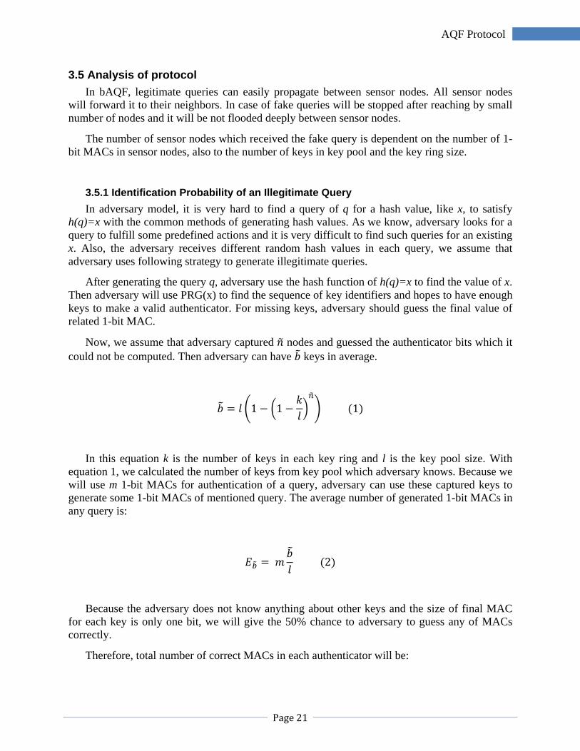
3.5.1 Identification Probability of an Illegitimate Query In adversary model, it is very hard to find a query of q for a hash value, like x, to satisfy

h(q)=x with the common methods of generating hash values. As we know, adversary looks for a query to fulfill some predefined actions and it is very difficult to find such queries for an existing x. Also, the adversary receives different random hash values in each query, we assume that adversary uses following strategy to generate illegitimate queries.

After generating the query q, adversary use the hash function of h(q)=x to find the value of x. Then adversary will use PRG(x) to find the sequence of key identifiers and hopes to have enough keys to make a valid authenticator. For missing keys, adversary should guess the final value of related 1-bit MAC.

Now, we assume that adversary captured nodes and guessed the authenticator bits which it could not be computed. Then adversary can have keys in average.

1 1 1

In this equation k is the number of keys in each key ring and l is the key pool size. With equation 1, we calculated the number of keys from key pool which adversary knows. Because we will use m 1-bit MACs for authentication of a query, adversary can use these captured keys to generate some 1-bit MACs of mentioned query. The average number of generated 1-bit MACs in any query is:

2

Because the adversary does not know anything about other keys and the size of final MAC for each key is only one bit, we will give the 50% chance to adversary to guess any of MACs correctly.

Therefore, total number of correct MACs in each authenticator will be:


2 2

2 1

2 3

Now, we can compute the probability that a node accepts and forward an illegitimate query.

4

With the combination of equation 3 and equation 4, we can have a better form for .

112 1 5

3.5.2 Propagation Probability of Illegitimate Queries Now, we can calculate the probability of accepting a fake query by a single node. But it is

different in real sensor networks. Sensor networks can show different behaviors depending on number of neighbors that any sensor nodes can have. The average number of neighbors for all sensor nodes called Node Density.

For simplification, we assume that each node has d neighbors and all of the neighbors have no connection with each other. If we want to draw a diagram to show how this network could be, the result is something like d-regular tree. In this diagram, propagation of fake query will start from root node. If any of neighbors can recognize that this query is illegitimate, it will stop forwarding query and none of its neighbors will receive this faked query. In this method, when a single query starts to process, it causes to create d descendants with probability of p. we know that the probability of not creating any descendants is 1 . With small numbers of producing entities, population will not be obvious. It will be clear if 1.

In real sensor networks, connections between sensor nodes have dissemination and it is more complex in comparison with d-regular tree and it looks like a branching process. We can consider the process of fake queries with . The given example in Figure 2 is for both d-regular tree and complex method. In this figure, after propagation of a fake query, only two nodes forward the fake query in d-regular tree, but in complex method, four of them forward the fake query and seven of them receive this fake query.

AQF Protocol

Figure 2: Propagation of a fake query (Left: in d-regular tree, Right: In branching process)

If we consider the propagation of fake queries which will be stopped in branching process, we will have following criterions:

1 6

And with combination of equation 5 and equation 6, we will have following equations:

1 1

12 1 7

log

log 1 12 1

8

3.5.3 Choosing Parameters As we can recognize, length of authenticator is depends on , , and . Parameters

named , , and will be controlled by administrator as long as will be controlled by adversary. Therefore, we need to find a way to choose , , and to have better performance in controlling fake queries for range of .

In this step, our suggestion is to start with node density. With high node density in sensor network, capacity will be decreased. On the other hand, if we choose a very low node density, connection between some nodes will be lost and network may become disconnected. As we want


to keep our network connected, we estimate the required node density as log (Feng & Kumar, 2004). As long as the number of neighbors in moderate network is still unclear, we consider 6 to 8 neighbors to be an ideal choice (Ni & Chandler, 1994 ).

Since we try to keep the ratio of in minimum, according to equation 1 and equation 8, we will have smaller amount for and , which is our target. Because we have to store key rings in sensor nodes and the amount of memory in sensor nodes are limited, we can not have big values for . In normal sensor nodes, we have only 10kB memory and if we estimate 80bits for a key length, we can have up to 200 keys in a key ring which this number will be the maximum value of . But, as we need to store key pool only in base station, we have no limitation for choosing the value of which will be key pool size.

Figure 3: Minimum authenticator size related to key ring size, key pool size and number of compromised nodes with node

density of 7.

Figure 3 shows the minimum required authenticator size for node density of 7. In this figure,

equation 8 is used for calculation of according to the number of compromised nodes and / (key pool size divided to key pool size). As we can see, there is always an optimal value of k/l for each particular value of compromised nodes. We are going to determine this optimal value.

If we consider as a fix ratio, we can simplify the equation 8 as bellow:

AQF Protocol

log

log 1 12 1

9

dd

log2

1 11

log 1 2 1 1 2 1 10

We can calculate optimal to have minimum :

dd 0

11 11

Therefore, we can calculate minimum authenticator size which is related to number of

captured nodes with using this equation.

log

log 1 12

11 1

12

Figure 4: Minimum Authenticator size related to compromised nodes with node density of 7


As Figure 4 shows, Minimum Authenticator size has an almost linear correlation with number of compromised nodes.

3.5.4 Analysis of Random Numbers Probability in bAQF Protocol In AQF protocol, we used random key pre-distribution to make key rings for sensor nodes. In

addition, we used a pseudo-random number generator function (like PRG ()) to choose authenticators which should be included in query. As long as we use random functions, always there is a chance to have duplicate keys in both key rings and authenticators. Because in each key ring the order of keys in not important, we can calculate the probability of repetition of a key in a key ring ( ) related to key pool size and key ring.

1!

! 13

The is probability of repetition for one key, and as we know there are keys in a key ring and it increase the chance of having duplicate keys times more. Then, can be the average value of duplicate keys in a key ring.

1!

! 14

On the other hand, we have several key rings in a sensor network and each two sample sensor nodes can have some common keys. It means we can have several duplicated keys in sensor network ( ).

1!

! 15

Because we use a large number of keys in key pool, , and parameters are ignorable. But if we had limited resources, for example smaller key pool for smaller network, the result could be changed and we should consider these values during calculation of different equations like .

Segment-based AQF

4. Segment-based AQF

4.1 Definitions Segment-based Authenticated Query Flooding shortly named sbAQF is a modified version of

bAQF. This version is designed to reduce the chance of fake queries for getting deeply into wireless sensor network.

In this version, we assume that the number of nodes could start from about tens and it can increase to hundreds or thousands nodes as well.

The targets of this algorithm are:

• Running on sensor nodes and geographical environment, the same as basic version. • Number of nodes will be the same • Needs for few updates instead of changing the program on sensor nodes which are

programmed to run bAQF for running the segment-based version. • Working against capturing, the same adversary as basic version.

4.2 System Model In this system model, we have the same number of sensor nodes distributed in same

geographical area. From electronically and communicational views, sensor nodes are the same with previous system model and also, adversary works the same, too. It means we have some captured node which can send fake queries into the WSN and we want to discover the fake queries as soon as possible.

4.3 Segment-based Key Assignment Before starting the algorithm, we need to assign cryptographic key from key pool to sensor

nodes. In segment-based form we use another strategy to choose which keys should assign to sensor nodes instead of using pseudo random generator.

Because we have no resource limitation in base station, we can choose our key pool big enough. In this way, first we choose a key ring size for our network, and then we multiply the key ring size to number of sensor nodes for calculating our key pool size. If we want to increase our key ring size, it is possible with increasing our key pool size as well. Therefore, key pool size will be divisible by number of nodes. Now, we can distribute the keys between sensor nodes. For this step, we make SN different segments with same number of keys in key Pool (

). We know that number of keys in each segment will be the same as our defined key ring size.


Figure 5. Segmentation in Key Pool

Then, we start assign individual keys of segments to sensor nodes. In this step we assign all keys from the segment with same identification number as sensor node (Figure 5). Each node can have the same number of independent keys from key pool in its key ring. The given pseudo-code shows how the algorithm works.

Algorithm sbAQF‐initial (NumberOfSensorNodes SN, KeyPool ( , … , ))

/* finding the number of keys in each key ring, k is Key Ring Size */

for =1 to do /* splitting to segments */ , … ,

end for for =1 to do /* assigning all keys from each segments to key rings*/ end for return

sbAQF‐initial Algorithm: The algorithm which should run before flooding

4.4 Segment-based Version In segment-based form, we can use basic form of algorithm in both base station and sensor

nodes. But, because the adversary may guess key numbers randomly without any care to segments, we can have alternatives for these algorithms to find if the query is coming from a segment-based station or not.

Segment-based AQF

As an alternative, if the number of sensor nodes was smaller than authenticator size, we can have authenticator encryption keys form different segments. It means in each segment we should use at least one encryption key which used to make an authenticator. In this case, we can use alternative algorithm in sensor nodes. With the alternative algorithm, each fake query which has no key from node’s segment will be rejected.

4.4.1 Base Station If the number of nodes was smaller than authenticator size, for more protection, we can use

the keys in different segments to make authenticator. For this job we used some random keys in each segment for making authenticator and we should have all the segments in this part of algorithm.

If we used this strategy in base station we also need to have some changes in sensor nodes to detect if all segments used in making authenticators and sensor node should reject the query if it can not find any authenticator which used encryptions keys in the segment with same identifier.

Our suggestion is to use the number of sensor nodes as a minimum value of authenticator size. If we choose smaller authenticator size in comparison with number of nodes, it may cause to forward a fake query in some sensor nodes which we did not used their segments to make query’s authenticator without any process. In this case, it is very easy for adversary to make a fake query to get ride of some nodes even without capturing some nodes or trying to guess an authenticator. Therefore for each segment we should have at least on Mac in our authenticator.

For selecting the order of keys in each segment to make our authenticator, we will use a pseudo-random generator function and we will check to have no key with generated identifier from before in same authenticator.

Algorithm sbAQF‐generate (Query q, Segments ( , … , ), AuthenticatorSize )

/* compute the hash value */ PRG init x

1 for = 1 to do if then 1 end if repeat PRG Until , … , 1 end for

, … , 1 bit MAC , , … , 1 bit MAC , return sbAQF‐generate Algorithm: The algorithm which should run in base station in segment‐based form


In this algorithm for generating authenticator of query, we will make a hash value for query the same as bAQF version and we will initialize our pseudo-random generator function with this value. Then, we try to select some keys to make our authenticator. For selecting keys, we will start from first segment. For choosing a key, we will use the PRG function to generate a sequence number of selected key within selected segment. If we had this key in our key sequence from before, we try our pseudo-random generator over and over to find a new key sequence number. When we find a new key in current segment, we will add it to our key list and we will move to next segment. If we reached to the last segment, we will start from first segment again and we will repeat this steps until we had enough keys to make the authenticator. This complex step is to satisfy different authenticator sizes and it can cover both the same size and the bigger size of authenticator in comparison with number of segments.

Finally, we will have all keys for making authenticator which contains a chain from 1-bit-MACs generated with different keys and hash value for the given query.

4.4.2 Sensor Nodes In Segment-based version of AQF, we have some changes in sensor nodes to detect whether

there is at least a Mac encrypted from the segment with same identifier in authenticator. We can use this alternative code when authenticator size is the same or bigger than number of segments (or number of sensor nodes).

This algorithm looks the same as bAQF version, but it is more powerful and also more complex. The first difference between these two versions is a flag value called segmentfoundflag. In this algorithm, first we make a hash value of query and we initialize PRG function with hashed value. Then, we will define a variable called segmentfoundvalue with initial value of false. Now, we can start our process on authenticator. Because we have the identifier number of node and number of sensor nodes in WSN, we can find the Macs in authenticator which are belong to current sensor node easily. We will start from first authenticator. In parallel, we will count the segment number of each Mac. If we reached to the end segment, we will continue our counting from first segment again. Whenever the segment number of counted Mac becomes equal with node identifier, we know that current Mac is belonging to our sensor node. Then, we would give true value to segmentfoundflag, because in this case we have a key in our key ring to check legitimacy of query. We make a 1-bit-MAC with existing key in our key ring and hash value. After that, we compare the result with the Mac in authenticator. If both values were not the same, we would reject the query because we assume that query is illegitimate.

After finishing this process for all Macs, we will check segmentfoundflag value. If it was false, the meaning is that we did not have any Mac encrypted with a key from our sensor node’s segment, therefore the query is fake and we will reject the query. Otherwise, we had a key from our segment in the query and value of related Mac has been matched with our key ring. In this case we assume that the query can be legitimate and we will forward it.

But how we can know which key in our key ring is belong to current Mac from our segment? For generating the sequence number of keys which will be used in authenticator, we will use PRG function with hashed value of query as the initial value. If we had a duplicate generated order number, we will just ignore it and we will generate another sequence number. The way of

Segment-based AQF

using pseudo-random generator for selecting key order is similar with ‘sbAQF-generate’ algorithm which we used for generating an authenticator for a query in previous part.

The following pseudo-code shows how this algorithm works:

Algorithm sbAQF‐verify (Query q, Authenticator ,KeyRing ( , … , ),SegmentNo , NumberOfNodes )

/* compute the hash value */ PRG init x

1 for = 1 to do if then 1 end if if then repeat PRG next Until , … , if 1 bit MAC , then return /* reject the query */ end if end if 1 end for if then return /* reject the query, because no key from sensor node’s segment founds in query */ end if return /* forward the query */

sbAQF‐verify Algorithm: The algorithm which can run in sensor nodes as an alternative

4.5 Analysis of Segment-based Version In this version, a legitimate query never be stopped with any nodes and it can reach to

destination easily. But an illegitimate one will be detected very fast. As we will discuss, different parameters can change the chance of detecting of an illegitimate query.


4.5.1 Identification Probability of a Fake Query As long as there is no duplicate key in key rings, adversary can not use captured nodes’ key

rings to make fake query. The only remaining chance is guessing. Because we generate only one bit as the result of hash value encryption, we assume that adversary can have only 50% chance to guess the related Mac correctly. If there were no captured node, adversary must guess m bits (m is authenticator size) with 50% chance as an authenticator. The chance will be 1/2 . But we have to discuss in a general form. Let us assume that adversary have access to capture nodes. On the other hand, we can have a big authenticator size in comparison with number of nodes (SN). Therefore, adversary has to guess fewer Macs. The equation shows the probability F that adversary can generate a fake query which acts like a legitimate query.

F12

16

We choose the key ring size by dividing key pool between sensor nodes like and as was a fix value, we called it as parameter.

1 17

Hence, the new form of will be:

F 18

But, we know that we can not check all authenticators in a sensor node and we can just check Macs which are belonging to node’s segment. Since the number of Macs from nodes segment is equal to / and also , we have an equation for accepting and forwarding a fake query in a sensor node ( ) as following:

12

12 19

Segment-based AQF

4.5.2 Identification Probability of Fake Queries As we discussed in part 3.5.2, a sensor network looks like a branching process (Figure 2) and

the main parameter in this kind of complex methods is Node Density (d). Node density is average number of neighbors which any sensor node can have. We know that, if we want to stop a fake query, we should have the same as equation 6 in segment-based version too.

P d 1 20

And with combination of equation 19 and equation 20, we will have:

1 12 21

Also we can have an equation related to authenticator size.

log

22

As we can see, as has a reveres correlation with number of nodes, the minimum authenticator size is dependent to node density and number of nodes and it is independent to number of expecting compromised nodes.

4.5.3 Benefits and Limitations of using Segments Now, there is a question which is: what do you expect from segments? With segments, we

have no duplicate keys in a key ring as well as in whole sensor network and it decrease the chance of guessing keys for adversary. As we discussed before, adversary can capture some nodes. After capturing, adversary will have access to key rings of captured nodes. Duplicated keys make it easier to generate an authenticator for a fake query, because there is a chance to have same keys with adversary in different key nodes. But in segment-based method, only captured nodes have same keys in adversary and there is no more duplication in network.

Let us assume that adversary can capture 3 nodes. In a big sensor network with 1000 nodes, 3 captured nodes is only 0.3% of nodes, but in a small sensor network containing only 10 nodes this percentage is about 30%. On the other hand, it may not really important in big networks to detect a fake query after very few steps because it is a long way up to destination node, but in small networks after few step a fake query can reach to destination and in this case only a few percentage of improvement, like segmentation, can help for detecting of more illegitimate queries.


But, what are the limitations of sbAQF in comparison with basic version? As we discussed in previous parts, we need to know the identification number of node and total number of sensor nodes in our WSN for checking the legitimacy of query. This situation makes it hard to add some new nodes into the WSN. Although it is easy to generate some keys as the new nodes’ key rings and add them to our key pool, but we should update all nodes with new number of sensor nodes and it should be mentioned in generating new authenticators as well. Also, the number of nodes in bAQF is unreachable for adversary, but if the adversary captured some nodes running sbAQF, it is easy to fetch the number of nodes from them.

On the other hand, it is easier to change some keys in nodes with segments. Because we have only one copy of each key in WSN, it is easier to change them and their copies in key pool. This caused to have easier recovery process for detected captured nodes. Recovery is harder in basic version, since we can have some duplicate keys in other sensor nodes and we may need to check and reprogram all sensor nodes to recover compromised nodes.

Evaluation

5. Evaluation

5.1 Simulation For verifying our results and comparing between both basic and segment-based protocols, we

developed a simulator. Our simulator is based on Matlab software form Mathworks Company. The way of using and configuration of this simulator is included in Appendix B and C. We use the simulator several times and we repeat each step in at least 100 times. The given diagrams of simulator are the average of these simulations.

5.1.1 Comparing results For checking the simulator, first we tried to run simulator with same parameters given in our

AQF reference paper (Benenson, Freiling, Hammerschmidt, Lucks, & Pimenidis, 2006). As the result shows, we had almost the same results with our reference paper. Therefore we believe we did our simulation the same as our reference. Figure 6 shows our simulation results.

Figure 6. Simulation of given parameters in reference paper

As the result shows, With increasing the number of authenticators, algorithm can detect illegitimate queries better but the improvement is not depend to the number of nodes and main factors are authenticator size and node density. Also using a bigger key ring and a bigger key pool can help bAQF to find fake queries but because we have limited resource in sensor nodes, increasing the number of cryptographic keys may not a good suggestion. It is better to use given equations in chapter 3 to find minimum number of authenticators, key ring and key pool size for using in our sensor network as well as checking our results with simulator in different situations.


5.1.2 Simulation Results Since the aim of our simulation was to check the performance of both algorithms, we tried to

keep the values for both algorithms the same. As long as we had a fix size of key ring in sbAQF, we calculated key ring size with “KeyRingSize KeyPoolSize/NumberOfNodes” formula in bAQF algorithm as well.

Also, we used “passed nodes” values instead of “received nodes” value which used in our reference paper for bAQF (Benenson, Freiling, Hammerschmidt, Lucks, & Pimenidis, 2006). The reason was that when we can detect the fake query and we can stop it, it does not mater if we discover it in destination or some steps before. Number of received nodes is related to node density of sensor network. With higher node density, more sensors will receive a fake query. But the important value is how many of them will pass the query. To compare both algorithms, we split our simulated networks into two different groups.

First, we assume our wireless sensor network is a big one. It means we have hundreds of nodes and thousands encryption keys in key pool. In these kinds of networks, adversary may capture some nodes and use them and send some fake queries into the network, also because adversary can have a physical access to captured nodes, we assume that the adversary can have access to the keys which exist in captured nodes.

In big networks, According to our simulations, during using basic version of algorithm, the most important parameters are node density and authenticator size and curves are not so related to number of nodes. In segment-based version, strength of algorithm was almost the same as basic version with very small and very big authenticator sizes, but gradient of improvement curve was more. sbAQF shows a better improvement with increasing authenticator size in comparison with basic version.

Figure 7. Simulation result for big sensor networks

Evaluation

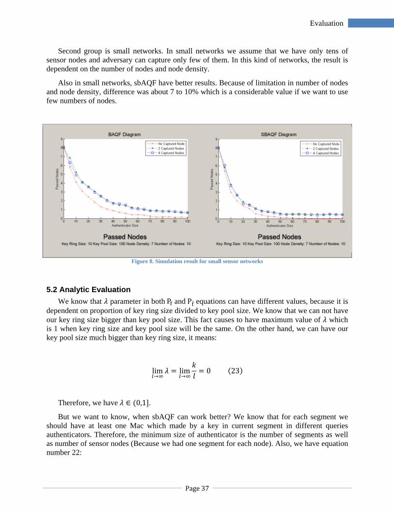
Second group is small networks. In small networks we assume that we have only tens of sensor nodes and adversary can capture only few of them. In this kind of networks, the result is dependent on the number of nodes and node density.

Also in small networks, sbAQF have better results. Because of limitation in number of nodes and node density, difference was about 7 to 10% which is a considerable value if we want to use few numbers of nodes.

Figure 8. Simulation result for small sensor networks

5.2 Analytic Evaluation We know that parameter in both P and P equations can have different values, because it is

dependent on proportion of key ring size divided to key pool size. We know that we can not have our key ring size bigger than key pool size. This fact causes to have maximum value of which is 1 when key ring size and key pool size will be the same. On the other hand, we can have our key pool size much bigger than key ring size, it means:

lim lim 0 23

Therefore, we have 0,1 .

But we want to know, when sbAQF can work better? We know that for each segment we should have at least one Mac which made by a key in current segment in different queries authenticators. Therefore, the minimum size of authenticator is the number of segments as well as number of sensor nodes (Because we had one segment for each node). Also, we have equation number 22:


In sbAQF: mlog d

22

On the other hand we have equation 9:

log

log 1 12 1

9

Figure 9. Diagram of Equation 25

In comparison between equation 22 and equation 9, we can consider that sbAQF needs less authenticator size and it works more efficient when:

Evaluation

log

log 1 12 1

log d 24

Or, when:

log 1 12 1λlog 2 1 25

It could be a complex statement to solve, but we tried to draw the diagram of this equation to check when this equation is correct. As we can see in Figure 9, the equation is always correct. Therefore sbAQF have a better performance in compression with bAQF which it proves our simulation results.

5.3 Advantages and Disadvantages of Protocols bAQF is much more fixable in comparison with sbAQF. We can adjust bAQF with different

amounts of resources. We can use this algorithm for hundreds or thousands of nodes with smaller key ring which is matched with our node’s free memory. With bAQF, it is easy to add a node to our WSN just with assigning some random keys from our key pool as the node’s key ring and we do not need to make any change in sensor nodes or queries. Number of nodes is transparent in network and adversary can not access to this value with capturing some nodes. But, recovery process for detected compromised nodes is hard and it may need to recheck or reassign key ring in all sensor nodes. Also it is easier for adversary to make a fake query because we have some duplicate keys in WSN.

On the other hand, sbAQF has a better performance in detection fake queries and make it harder for adversary to make a fake query. As long as we have no resource limitation in base station to have a big key pool size, the fix size of key rings is not an important issue. Recovery process of detected captured nodes is very easy, because we have only one copy of each key in WSN. But adding nodes to sensor network is hard and needs to reassign values to all sensor nodes for checking the legitimacy of query. Also, we need to have at least one Mac in authenticators for each sensor node and it cause to have big authenticators in big sensor networks.

Conclusion

6. Conclusion

In this work, we had a review of basic authentication query flooding algorithm in sensor networks which use probability to found faked queries in network and stop forwarding them before they reached by most of sensor nodes and only small part of network can receive the faked query and even they can find the query as a illegitimate query. This small part of network is not depended with number of sensor nodes in our wireless sensor network. With changing the parameters of network like key pool size, key ring size, authenticator size and node density you can tune the power of algorithm for different sensor networks.

For fine-tuning of algorithm in different WSNs, we made a simulator the simulated wireless sensor networks with different parameters values in different conditions and it is possible to find the best result on simulator diagrams after simulation. Also we compared our simulation result with the diagrams presented in AQF algorithm paper to be sure that the diagrams of our simulator are almost the same as diagrams of original paper.

Also we present a new version of this algorithm, named segment-based AQF. In this format, there is no need to have a big change in running application of sensor nodes, but with some changes in initialization step, we can improve the security in network. Our simulator can also use this algorithm to find better values for parameters. We used our simulator to compare both algorithms in different networks and we had better results for SBAQF.

For future studies, we offer a way which may improve this protocol. Our suggestion is to use salt value during of hashing query and it may make it harder to guess key identifiers of query or using the captured keys to generate authenticator, but it needs a way to protect the salt during communicating or capturing a node. Also we can check if it is better to have a fix salt or using several salt values (some thing like salt pool!). But we believe this way may need more resources in sensor nodes, also it should be used if it makes a big difference in security performance of protocol.

References

7. References

Benenson, Z., Freiling, F. C., Hammerschmidt, E., Lucks, S., & Pimenidis, L. (2006). Authenticated Query Flooding in Sensor Networks. 21st IFIP International Information Security Conference SEC 2006 (pp. 1-12). Karlstad, Sweden: Karlstad University.

Canetti, R., Garay, J., Itkis, G., Micciancio, D., Naor, M., & Pinkas, B. (1999). Multicast Security: A Taxonomy and Some Efficient Constructions. IEEE INFO-COM'99 (pp. 708-716). New York NY, USA: IEEE.

Eschenauer, L., & Gligor, V. D. (2002). A key-management scheme for distributed sensor networks. Proceedings of the 9th ACM Conference on Computer and Communications (pp. 41–47). Washington DC: ACM Press.

Feng, X., & Kumar, P. R. (2004). The Number of Neighbors Needed for Connectivity ofWireless Networks. Urbana, IL: Kluwer Academic Publishers.

Ganeriwal, S., Capkun, S., Chih-Chieh, H., & Srivastava, M. B. (2005). Secure time synchronization service for sensor networks. Proceedings of the 4th ACM workshop on Wireless security, (pp. 97-106). New York, NY, USA: ACM Press.

Intanagonwiwat, C., Govindan, R., Estrin, D., Heidemann, J., & Silva, F. (2003). Directed Diffusion forWireless Sensor Networking. IEEE/ACM , 2-16.

Madden, S., Franklin, M. J., & Hellerstein, J. M. (2003). The Design of an Acquisitional Query Processor For Sensor Networks. Proceedings of the 2003 ACM SIGMOD International Conference on Management of Data (pp. 491-502). New York NY, USA: ACM Press.

Moteiv. (2006, November 13). Tmote Sky Datasheet. Retrieved April 25, 2007, from Moteiv Wireless Sensor Networks: http://www.moteiv.com/products/docs/tmote-sky-datasheet.pdf

Ni, J., & Chandler, S. A. (1994 ). Connectivity properties of a random radio network. Communications, IEEE Proceedings , 289 - 296.

Perrig, A., Szewczyk, R., Wen, V., Culler, D., & Tygar, J. D. (2002). SPINS: Security Protocols for Sensor Networks. Berkeley, CA: University of California, Berkeley.

Says, S., & Preneel, B. (2005). Efficient cooperative signatures: A novel authentication scheme for sensor networks. 2nd International Conference on Security in Pervasive Computing (pp. 86-100). Boppard, Germany: Springer.

Zhu, S., Xu, S., Setia, S., & Jajodia, S. (2003). Establishing pairwise keys for secure communication in ad hoc networks: a probabilistic approach. 11th IEEE International Conference on Network Protocols (pp. 326- 335). Atlanta GA: IEEE Computer Society Conference Publishing Services.

APPENDIXES

Appendix A. AQF Simulator

Appendix A. Index

µ

µTESLA ..................................................................... 15

A

AQF Simulator .......................................................... 57 AQFConfig.m ................................................ 50, 51, 57 AQFFlooding.m ........................................................ 55 AQFResult.mat ......................................................... 51 ASCII Editor .................................................. 50, 51, 57 Authenticated Broadcast ......................................... 15 Authenticated Multicast .......................................... 15 Authenticated Query Flooding ................................ 13 Authenticator .................................................... 15, 20 Authenticator Size ................................................... 57

B

bAQF ........................................................................ 19 Base Station ............................................................. 13 Basic Authenticated Query Flooding ....................... 19 Bounding Method .................................................... 58

C

Captured Nodes ....................................................... 57 Command Mode ...................................................... 51 Command Window .................................................. 51 Communication Range ............................................ 57 Current Directory Window ...................................... 50

D

Directed Diffusion .................................................... 13 Draw Button ...................................................... 53, 55 Draw Diagram .......................................................... 53 Draw Diagram Button ........................................ 51, 54

F

Fake Query ............................................................... 17 Flooding ................................................................... 13

H

Hash Function .......................................................... 20

I

Illigitimate Query ..................................................... 17 Initial Value .............................................................. 57 Interface Mode .................................................. 51, 58

K

Key Pool ................................................................... 18 Key Pool Size ............................................................ 57

Key Ring ................................................................... 18 Key Ring Size ............................................................ 57

L

Legitimate Queries .................................................. 17

M

Matlab ............................................................... 35, 49 Matlab Editor ........................................................... 50

N

Node Density ............................................... 22, 33, 58 Number of Curves .............................................. 53, 58 Number of Retries ................................................... 58 Number of Sensors .................................................. 57 Number of Steps ................................................ 52, 58

P

Passed Nodes ........................................................... 54 PDA .................................................................... 13, 17 Pre‐configured Mode .............................................. 51 Pre‐confured Mode ................................................. 51

R

Received Nodes ....................................................... 54 Run Simulation Button............................................. 51

S

sbAQF....................................................................... 27 SBAQFFlooding.m .................................................... 55 Second Step ............................................................. 57 Segment ................................................................... 27 Show Result Network .............................................. 53 Show Result Network Button .................................. 51 Simulation Parameters ............................................ 52 SPINS ........................................................................ 15 Step .......................................................................... 57

T

TinyDB ...................................................................... 13 Tmote Sky ................................................................ 17

V

Visual Mode ............................................................. 51

W

Wireless Sensor Networks ....................................... 13 Working Directory ................................................... 49 Workspace Window................................................. 51

Appendix B. AQF Simulator


AQF Simulator is an application which we developed to evaluating the results of these protocols. This simulator is developed under Matlab environment and it works like an internal function.

For running the AQF Simulator, you should have the Matlab installed on your system. We used Matlab R2006a for this simulation, although it also works with some older versions. For running the simulator you should have at least Java Runtime Environment (JRE) installed on same machine.

1. Installation For installing the simulator, first you should find your working directory of your Matlab.

After running Matlab application, you can found it on your matlab toolbar, under the menus. The box with title of Current Directory shows you your working folder (Figure 10).

Working Directory can be different from system to system. Also you can change it very easily. But for running the simulator it should be match with your simulator installation directory.

Figure 10: Current Directory in Matlab Environment

We assume that we are using a Matlab application on Microsoft Windows Machine. In this case, Default current directory will be some thing like:

C:\Program Files\MATLAB\R2006a\work


We use this folder for installing the simulator. Just we have to browse this folder and copy the simulator files into this folder. After finishing, it will be ready to run.

This files should be in your working directory after installation:

• AQFCheckConfig.m: This file is used for testing if the default parameters or entered parameters using command line are matched with requirments or not.

• AQFCmdConfig.m: This part is for configuration of simulator form command line. • AQFConfig.m: This file is configuration file of simulator. Use an ASCII editor for

editing this file and run the simulator in different modes. For underestanding better of the parameters, please read Appendix C.

• AQFDiagram.fig: This file is visual part of drawing digram function of simulator. After simulation you can see your final curves using this part.

• AQFDiagram.m: this part is code part of AQFDiagram.fig. The application which runs behind digram part is included in this file.

• AQFDrawNetwork.fig: This file is used to draw sensors in simulated geographical area to preview which nodes passed a fake query and which nodes stop them. Connection between sensor nodes are also included in this picture.

• AQFDrawNetwork.m: this file contain the source code of AQFDrawNetwork.fig. • AQFFlooding.m: This part is one of the most important files of simulator. Flooding

of fake query will be simulated using this file. • AQFGui.fig: This file is the visual user interface of simulator. Using this file you can

easily change the parameters and draw different diagrams. • AQFGui.m: Code behinds of visual user interface are in this file. • AQFNetworkGenerator.m: This file is used to generate random wireless sensor

networks in each simulation. • AQFSim.m: The main rootin of simulator is in this file. For running the simulator

you will need to call rootins which are included in this file. • AQFTaskManager.m: Simulation tasks and sequencese of running applications will

be managed using this part of simulator.

All of the simulator files should be in same place. If during the simulation, simulator can not find any of these file, it stop simulating and exit the application with a message for reinstallating the simulator.

2. Configuration After installation step, you can change defualt values using a normal ASCII editor or Matlab

editor which is included in Matlab Environment. You can see the file name on your Current Directory Window on top-left corner of your Matlab environmet. If this window is not visible on your Matlab, you can active it from Desktop menu. By double clicking on any file name, you can open it on Matlab Editor.

Configuration file of simulator named AQFConfig.m. With a double click on its name, you can easily edit and change default values of simulator (Figure 11). For reading more about AQFConfig.m, check Appendix C.


Figure 11: Editing AQFConfig.m in Matlab Editor

3. Running Simulator There are three different ways to run simulator, Pre-configured mode, Command Mode and

Visula mode. You can set the running mode with parameeter of Interface_Mode in AQFConfig.m file.

For executing the simulator, we just need to type AQFSim. Capital and small letters should type in correct way, otherwise Matlab may shows you a warning message. Depend on Interface Mode of simulator, it run in different ways.

In pre-configured mode, the simulation will run without any question. On Command Window, you can follow the steps of simulation. Finally, the simulation answers are reachable by loading AQFResult.mat file.ou just need to type “load AQFResult” to load simulation results into Matlab Workspace Window.

In command mode, everything is the same with pre-configured mode, except one. Before starting simulation, you can enter your values for different parameters on command window and AQF Simulator gives you some hints to enter correct values. After this step, simulation will be started.

Visual mode is the most complex mode in AQF Simulator. In this mode, after typing the AQFSim command, you will see the grphical user interface of simulator preloaded by default values. You can easily change the values or use menu bar to load or save them (Figure 12).

After setting up the paameters, press on Run Simulation button to start simulation and wait until finishing the simulation steps. After execution, Show Result Network and Draw Diagram buttons will be available.


Figure 12: AQF Simulator in Visual Mode

4. Simulator Parameters Nodes parameters section have 4 rows and 3 columns (Figure 12). Each of the rows shows

one of important parameters in simulation, such as key pool size, key ring size, authenticator size and number of captured nodes.

First column shows the initial value of these parameters. Therefore, simulation will start with initial values. Because AQF is using probabilistic methods, AQF have a retry parameter called Number of Retries in Each Step. With this parameter, You can retry same simulation for many time and the final answer should be the average of answers.

The result of simulation will be some curve. We can make this curve from each view which we want to check the algorithm. The step value of parameters, shows the gap between each level of curve (Figure 13). The number of steps parameter shows the number of level on each curve.


Figure 13: Initial, Step and 2nd Step Values

Number of curves parameter shows the number of curve in final diagram. In each curve, the start value of each parameter is its initial value added by 2nd Step Value multiply by curve number minus 1 (Figure 13).

1

5. Previewing of Simulated networks After finishing the simulation, Show Result Network and Draw Diagram buttons will be

available. With clicking on Show Result Network button the new windows will be shown which using that window you can preview the simulated sensor networks. In this window, you can see the sensors like black circles, connection between sensors with cyan lines and base station with a blue circle. If any node can recognize that the sent query is faked and stop forwarding it, it shows with red color on map and if the node can not recognize the fake query and forward that the color will be green (Figure 14). Therefore remain circles with black color do not receive any fake query.

Slider bar under this window helps you to choose between different simulated networks. Because for simulation results, simulator needs to compare different results of different networks together. If you saw any unclear point the result diagram you can check the simulated networks. When you change the position of slider bar, you can see the selected network name on top of slider bar. If you found your choice, with clicking on Draw button, you can see the related network in few seconds.


Figure 14: Preview of Simulated Sensor Networks

6. Simulated Diagram Using Draw Diagram Button, you can reach AQF Simulator Diagram window. Final result

of simulation will be shown on this window. You can choose the different parameters of key pool size, key ring size, authenticator size and number of captured nodes as the affected parameter in X axis and received nodes or passed nodes for Y axis.

When you select the received nodes as the parameter of Y axis, the value of each point shows the number of nodes which received the query, even they found the query as a faked one. But if you select passed nodes, the value will be the number of sensor nodes which recognize the query as a legitimate one and forward that throw the network. This choice can show the power of algorithm in finding illegitimate queries much better than received nodes parameter (Figure 15).


Figure 15: AQF Simulator Diagram

After choosing the parameters, you only need to press Draw Button to saw the final diagram of simulation. After drawing different parameters, you also can change the parameters and redraw the diagram.

7. Simulation of Segment-based AQF By default, the AQF Simulator simulates the bAQF algorithm. But it is easy the change the

mode of simulator to work with sbAQF algorithm. The only work you need is to change AQFFlooding.m file with the version which used for sbAQF simulation. The file named SBAQFFlooding.m. You can change the name of AQFFlooding.m file to something like BAQFFlooding.m and rename the SBAQFFlooding.m to AQFFlooding.m. From now, the simulator use Segment-based algorithm instead of basic version.

Also you can have both versions installed in different directories. For example Basic version in BAQF directory and a copy of modified version in another directory named SBAQF. In this case you can easily switch between the simulation algorithms with just changing Current Directory value in your Matlab (Figure 10).

Appendix C. AQF Simulator Configuration File

Appendix C. AQF Simulator Configuration File

For changing the default values and configurations in AQF Simulator, you can easily change them in AQFConfig.m file which in exists in installed folder of simulator. You can use any ASCII editor for changing them.

The most important things to caution are:

• Do not change the parameter names and do not delete them. This may cause of some errors or deadlocks during simulation.

• You can only replace the values with a new value within the given range • Do not change or remove function prototype and saving part in the beginning and

ending part of file which are notified with comments

Here we need to describe steps and second steps in simulator. Final result of simulator will be some curves which show together on same axis. Step is the value which adds in each step on same curve. For example, first curve will start with initial value and in each step; step value will be added and makes the next point. 2nd-step value shows the difference between curves. Second curve will start from initial value added with 2nd-step value (check Figure 13). If you want to keep an attribute fixed, set the step and 2nd_step values of that attribute on 0.

Keypool_Size is the variable which assigns the number of keys which they are in Key Pool. Key pool size should be bigger that Key ring size and Authenticator size, other wise simulator will face to a deadlock. Keypool_Step and Keypool_2ndStep are its step gaps. The values should be positive or zero.

Keyring_Size is the number of cryptographic keys which they are available on any sensor node. Key ring size should be smaller that Key pool size, other wise simulator will face to a deadlock. Keyring_Step and Keyring_2ndStep are its step gaps.. The values should be positive or zero.

Authenticator_Size is the number of 1-bit MACs which attached to the query to verify if the query is legitimate or not. Authenticator size should be smaller that Key pool size, other wise simulator will face to a deadlock. Authenticator_Step and Authenticator_2ndStep are its step gaps. . The values should be positive or zero.

Captured_Nodes is the number of nodes which we assume that the adversary captured them. The key ring of random captured node will be reachable by adversary and we believe adversary can guess them correctly. Captured_Nodes_Step and Captured_Nodes_2ndStep are its step gaps . The values should be positive or zero.

Number_of_Sensors is a variable which clear the number of sensor nodes in simulated wireless sensor network. The number should be at least 1.

Communication_Range is the maximum effective distance between sensor nodes. If the direct distance between two sensor nodes was less than this number, they can forward received queries for each other. If this number sets to zero, it means none of the sensor networks have no connection with other nodes.


Bounding_Method is the variable which clears that how the geographical area of our simulation should be. We can assign only 0 or 1 as value to this parameter. The meanings of these values are:

0. Area_Length and Area_Width will be calculating using different parameters of Node_Density, Number_of_Sensors and Communication_Range automatically. The Assigned values to Area_Length and Area_Width in configuration file will be ignored and replaced with new calculated values. In this method area size will set automatically. (Default)

1. With this value, the size of geographical Area will assign from Area_Length and Area_Width. In this method Node_Density parameter has no effect in simulation.

Node_Density assign the normal number of neighbors which we will have in average for each sensor node. This number should be at least 1. This variable has effect only when Bounding_Method was set to 0.

Area_Length and Area_Width set the geographical area size of our simulation. These parameters should be a positive number and they have effect only when Bounding_Method was set to 1.

Number_of_Retries is the number of execution in each step with same parameters. Because AQF is a probabilistic protocol, it is better to retry each simulation with fix values for several times. Final result will be the average of answers. Number_of_Retries should be at least 1.

Number_of_Steps the number of times which we want to change our parameters. With the number of steps, step parameter of each attribute will be added to its old value to calculate next value for simulation. Read more details on introduction of this appendix or check Figure 13. This number should be at least 1.

Number_of_Curves is the number of curves which we will have on diagrams. It will be calculate with adding 2nd Step to default values and resimulate from scratch. All the curves will be shown on same axis. Number_of_Curves should be at least 1.

Interface_mode shows the mode which we want to run the simulator. With this parameter we can choose different ways of entering the parameters into the simulator. This parameter is made for running the simulator under different systems or platforms. Interface_Mode can have these values:

0. In this mode, Simulator runs without interface and it just use the default values which are included in this file (AQFConfig.m)

1. Text mode interface will be available with this parameter. After running the simulator, it will ask all the parameters using command line.

2. Visual mode is the most powerful interface of AQFSimulator. With this parameter you can easily change the parameters, load and save the results, draw diagrams and check the simulated sensor networks graphically.

The default value of Interface_Mode is 0.

authentication of queries in wireless sensor networks

Documents