austrian climate research program - tu wien · acrp ‐ austrian climate research program ......

1

Austrian research cooperation

Austrian Climate Research Programme ACRP 3nd Call

Funded by Climate and Energy Fund

ACRP ‐ Austrian Climate Research Program

Power through Resilience of Energy Systems: Energy Crises,

Trends and Climate Change (PRESENCE)

Contributions to Work packages

4 – Hydrology and hydropower

5 – Availability of cooling water for thermal power plants and the industry

by

Institute of Water Management, Hydrology and Hydraulic Engineering (IWHW)

University of Natural Resources and Life Sciences, Vienna (BOKU)

Project management: Em.O.Univ.Prof. Dipl.Ing. Dr. Hans Peter Nachtnebel

Authors: DI Philipp Stanzel, DI Mathew Herrnegger

Draft March 2013

2

Table of Content

1. Introduction ............................................................................................................................ 4

2. Methods .................................................................................................................................. 6

2.1. Water balance simulations ...................................................................................................... 6

2.2. Changes in runoff due to precipitation and temperature changes (Runoff elasticity) ........... 8

2.3. Analyses of river runoff time series from scenario simulations .............................................. 8

2.3.1. Analysis of low flow periods ......................................................................................................... 9

2.3.2. Long‐term persistence and periodicity ....................................................................................... 11

2.4. Impact of climate change on alpine reservoirs ..................................................................... 12

2.5. Water temperature ............................................................................................................... 14

2.6. Groundwater recharge .......................................................................................................... 14

2.7. Trends in runoff in Europe .................................................................................................... 15

3. Input data .............................................................................................................................. 16

3.1. Corrections of RCM data ....................................................................................................... 16

3.2. Climate change signals .......................................................................................................... 16

4. Results ................................................................................................................................... 19

4.1. Performance of the water balance model ............................................................................ 19

4.1.1. Simulations with observed input data ........................................................................................ 19

4.1.2. Simulations with corrected climate model control runs............................................................. 21

4.2. Runoff elasticity ..................................................................................................................... 23

4.3. Spatial patterns of change in local runoff ............................................................................. 26

4.4. Changes in river runoff .......................................................................................................... 30

4.4.1. Mean runoff ................................................................................................................................ 30

4.4.2. Analysis for run‐of‐river power plants ........................................................................................ 31

4.4.3. Runoff seasonality ...................................................................................................................... 34

4.4.4. Low flow runoff under climate change conditions ..................................................................... 37

4.4.5. Low flow runoff for shorter periods than a month: Mean annual 7‐day minimum flow ........... 40

4.4.6. Time of occurrence of low flow periods ..................................................................................... 42

4.4.7. Low flow duration under climate change conditions ................................................................. 43

4.4.8. Long‐term persistence and periodicity in simulated runoff time series ..................................... 45

4.5. Alpine reservoirs .................................................................................................................... 52

4.5.1. Gepatsch ..................................................................................................................................... 52

4.5.2. Sellrain‐Silz .................................................................................................................................. 59

3

4.5.3. Kaprun‐Uttendorf ....................................................................................................................... 60

4.6. Water temperature ............................................................................................................... 61

4.7. Groundwater recharge .......................................................................................................... 62

4.8. Trends in runoff and hydropower production in Europe ...................................................... 65

4.8.1. Mean runoff and hydropower potential ..................................................................................... 65

4.8.2. Seasonal changes ........................................................................................................................ 67

4.8.3. Low flow ...................................................................................................................................... 70

5. Conclusions ........................................................................................................................... 73

6. References ............................................................................................................................. 75

7. List of Figures ......................................................................................................................... 78

8. List of Acronyms .................................................................................................................... 84

9. Annex – Comments on the delivered runoff simulation time series ........................................ 85

9.1. Delivered runoff simulation time series ................................................................................ 85

9.2. Estimation of the Swiss and German Inn and the German Danube ...................................... 88

9.3. Estimation of a typical hydrological regime shift for German hydropower production ....... 89

4

1. Introduction

The core objective of the overall project “PRESENCE – Power through Resilience of Energy Systems:

Energy Crises, Trends and Climate Change” is to provide measures and pathways how to increase the

resilience of energy systems in the view of climate change, possible trends and energy crises as well

as the transformation of our energy system into a low‐ and zero carbon future for the Austrian case.

In order to follow this basic idea of the project, the following sub‐objectives of “PRESENCE” have

been defined:

‐ Identify and quantify the impact of climate change on energy systems. This includes a

detailed description and modeling of energy systems in a highly disaggregated way. This will

imply modeling the climate sensitivity of (1) hydro power, (2) electricity generation, storage

and transmission, (3) heating and cooling of buildings and (4) selected aspects of cooling

water availability for thermal power plants and industrial energy related processes.

‐ Identify and quantify the possible impact of other exogenous trends, developments and

possible shocks on energy systems.

‐ Further elaborate the methodological concept of resilience for the case of energy systems.

‐ Further develop methodological concepts for assessing the impact of extreme events on

energy systems.

‐ Identify steps and concepts for increasing the resilience of energy systems and quantifying

the impact of transition paths and measures on resilience indicators.

‐ Investigate economic aspects of adaptation measures and discuss strengths and limitations

of economic concepts for assessing cost and benefits of adaptation measures.

This report summarizes the contributions of the IWHW group to Workpackage (WP) 4 – Hydrology

and hydropower – and WP 5 – Availability of cooling water for thermal power plants and the

industry. The main objectives of these investigations are:

‐ Assess the expected impact of climate change on the hydrology of Austria.

‐ Analyse electricity generation of hydropower in different climate scenarios.

‐ Investigate cooling water availability under climate change conditions.

The main tool to achieve these objectives is a detailed spatio‐temporal hydrological model for

Austria. After calibration for a period in the 20th century, the model is run with climate change

scenario input data for the 21st century. Climate scenarios provided by the latest generation of

climate models are prepared and corrected in WP 1 – Climate models and scenarios. Trends in the

resulting hydrological scenarios are analysed, with special focus on impacts on hydropower

production and cooling water availability. The simulated time series of runoff will also be used as

input in subsequent detailed modeling of hydropower production in an energy model based on an

inventory of all major hydropower stations (by the Energy Economics group, EEG). In addition to the

detailed investigation of expected changes in hydrology and hydropower production in Austria,

external factors related to hydropower production in Europe are investigated and summarized.

5

Of the analyses of climate change impact presented here, the following points have special relevance

for hydropower production (WP4):

‐ Continuous monthly runoff time series of the 21st century for the main Austrian rivers

‐ Mean runoff and seasonality

‐ Low flow runoff, time of occurrence and duration of low flow periods

‐ Specific analysis for run‐of‐river power plants

‐ Specific analysis for alpine reservoirs

‐ Trends in runoff and hydropower production in Europe

For the investigation of cooling water availability under climate change conditions (WP5), the

following issues discussed here are of special relevance:

‐ Mean runoff and seasonality

‐ Low flow runoff, time of occurrence and duration of low flow periods

‐ Water temperature

‐ Groundwater recharge

‐ Trends in runoff in Europe

6

2. Methods

2.1. Water balance simulations

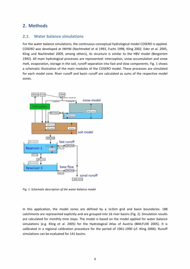
For the water balance simulations, the continuous conceptual hydrological model COSERO is applied.

COSERO was developed at IWHW (Nachtnebel et al 1993, Fuchs 1998, Kling 2002, Eder et al. 2005,

Kling und Nachtnebel 2009, among others), its structure is similar to the HBV model (Bergström

1992). All main hydrological processes are represented: interception, snow accumulation and snow

melt, evaporation, storage in the soil, runoff separation into fast and slow components. Fig. 1 shows

a schematic illustration of the main modules of the COSERO model. These processes are simulated

for each model zone. River runoff and basin runoff are calculated as sums of the respective model

zones.

Fig. 1: Schematic description of the water balance model

In this application, the model zones are defined by a 1x1km grid and basin boundaries. 188

catchments are represented explicitly and are grouped into 16 river basins (Fig. 2). Simulation results

are calculated for monthly time steps. The model is based on the model applied for water balance

simulations (e.g. Kling et al. 2005) for the Hydrological Atlas of Austria (BMLFUW 2005). It is

calibrated in a regional calibration procedure for the period of 1961‐1990 (cf. Kling 2006). Runoff

simulations can be evaluated for 141 basins.

7

Fig. 2: 188 Austrian catchments represented in the water balance model, grouped into 16 river basins

The impact of climate change on the terrestrial water balance is investigated using precipitation and

temperature data resulting from climate model simulations as input. Water balance modeling results

of future periods under climate change conditions can then be compared with the reference

simulations for 1961‐1990.

For the application with climate model data, the model is adapted regarding the simulation of

evaporation, snow melt and glaciers.

Evaporation is calculated with the method of Thornthwaite (Thornthwaite and Mathers 1957). This

method only requires temperature as input. Therefore, the climate signal in the temperature data is

considered in the calculations of evaporation. Other methods, like the method of Budyko (1974) that

is originally implemented in the water balance model, need other input data which is not readily

available from climate models or is more complicated to correct than temperature data. In the

Thornthwaite method, effects of temperature and radiation are combined in an empirical approach.

The use of the Thornthwaite method with climate change scenario temperatures implies a linear

relationship, with potential evaporation rising as much as temperature. However, radiation, which is

then implicitly assumed to increase in the same way as temperature, is not expected to generally

increase. This might lead to a small, but systematic overestimation of potential evaporation.

In the calculation of snow melt, the variability of daily temperature around the monthly mean is fixed

with a value calculated from data of the calibration period 1961‐1990. In applications for this period,

time series of observed daily temperature are used, which are not available for monthly scenario

data.

A simple glacier model is applied in combination with the water balance model for the scenario

simulations. Glaciers are not considered in earlier applications, and are also not included in the

simulations of the reference period of 1961‐1990. The glacier melt simulated by the glacier model is

therefore the additional contribution by glaciers that so far did not contribute to runoff in

1961‐1990. Model zones which are mostly snow covered in summer in 1961‐1990 are therefore

considered as glacierized (see Fig. 8 in chapter 2.4). Glacier melt is calculated with a temperature

8

index method. Lateral mass movement is not considered. Ice thickness in one model zone is

distributed according to a log normal distribution. Ice volumes are estimated based on information

by Kuhn et al. (1999) and Span et al. (2005).

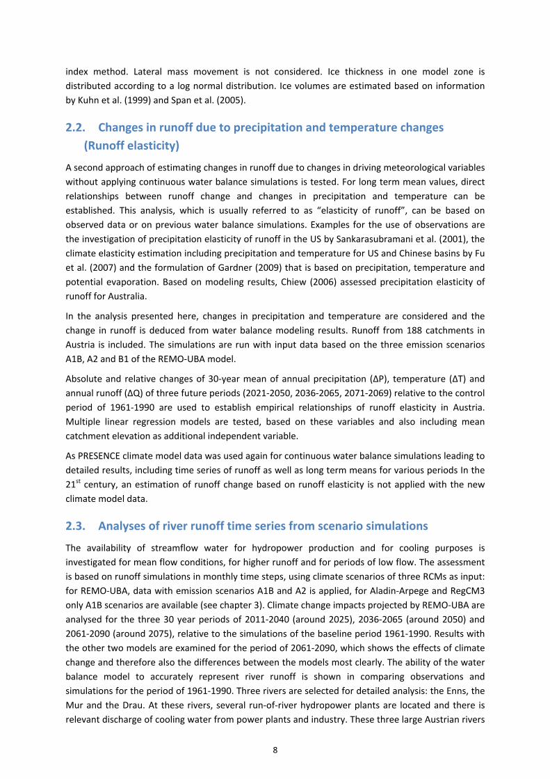
2.2. Changes in runoff due to precipitation and temperature changes

(Runoff elasticity)

A second approach of estimating changes in runoff due to changes in driving meteorological variables

without applying continuous water balance simulations is tested. For long term mean values, direct

relationships between runoff change and changes in precipitation and temperature can be

established. This analysis, which is usually referred to as “elasticity of runoff”, can be based on

observed data or on previous water balance simulations. Examples for the use of observations are

the investigation of precipitation elasticity of runoff in the US by Sankarasubramani et al. (2001), the

climate elasticity estimation including precipitation and temperature for US and Chinese basins by Fu

et al. (2007) and the formulation of Gardner (2009) that is based on precipitation, temperature and

potential evaporation. Based on modeling results, Chiew (2006) assessed precipitation elasticity of

runoff for Australia.

In the analysis presented here, changes in precipitation and temperature are considered and the

change in runoff is deduced from water balance modeling results. Runoff from 188 catchments in

Austria is included. The simulations are run with input data based on the three emission scenarios

A1B, A2 and B1 of the REMO‐UBA model.

Absolute and relative changes of 30‐year mean of annual precipitation (ΔP), temperature (ΔT) and

annual runoff (ΔQ) of three future periods (2021‐2050, 2036‐2065, 2071‐2069) relative to the control

period of 1961‐1990 are used to establish empirical relationships of runoff elasticity in Austria.

Multiple linear regression models are tested, based on these variables and also including mean

catchment elevation as additional independent variable.

As PRESENCE climate model data was used again for continuous water balance simulations leading to

detailed results, including time series of runoff as well as long term means for various periods In the

21st century, an estimation of runoff change based on runoff elasticity is not applied with the new

climate model data.

2.3. Analyses of river runoff time series from scenario simulations

The availability of streamflow water for hydropower production and for cooling purposes is

investigated for mean flow conditions, for higher runoff and for periods of low flow. The assessment

is based on runoff simulations in monthly time steps, using climate scenarios of three RCMs as input:

for REMO‐UBA, data with emission scenarios A1B and A2 is applied, for Aladin‐Arpege and RegCM3

only A1B scenarios are available (see chapter 3). Climate change impacts projected by REMO‐UBA are

analysed for the three 30 year periods of 2011‐2040 (around 2025), 2036‐2065 (around 2050) and

2061‐2090 (around 2075), relative to the simulations of the baseline period 1961‐1990. Results with

the other two models are examined for the period of 2061‐2090, which shows the effects of climate

change and therefore also the differences between the models most clearly. The ability of the water

balance model to accurately represent river runoff is shown in comparing observations and

simulations for the period of 1961‐1990. Three rivers are selected for detailed analysis: the Enns, the

Mur and the Drau. At these rivers, several run‐of‐river hydropower plants are located and there is

relevant discharge of cooling water from power plants and industry. These three large Austrian rivers

9

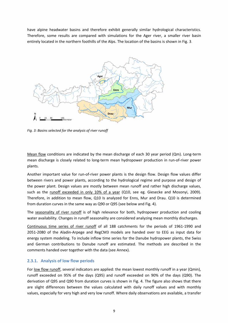
have alpine headwater basins and therefore exhibit generally similar hydrological characteristics.

Therefore, some results are compared with simulations for the Ager river, a smaller river basin

entirely located in the northern foothills of the Alps. The location of the basins is shown in Fig. 3.

Fig. 3: Basins selected for the analysis of river runoff

Mean flow conditions are indicated by the mean discharge of each 30 year period (Qm). Long‐term

mean discharge is closely related to long‐term mean hydropower production in run‐of‐river power

plants.

Another important value for run‐of‐river power plants is the design flow. Design flow values differ

between rivers and power plants, according to the hydrological regime and purpose and design of

the power plant. Design values are mostly between mean runoff and rather high discharge values,

such as the runoff exceeded in only 10% of a year (Q10, see eg. Giesecke and Mosonyi, 2009).

Therefore, in addition to mean flow, Q10 Is analyzed for Enns, Mur and Drau. Q10 is determined

from duration curves in the same way as Q90 or Q95 (see below and Fig. 4).

The seasonality of river runoff is of high relevance for both, hydropower production and cooling

water availability. Changes in runoff seasonality are considered analyzing mean monthly discharges.

Continuous time series of river runoff of all 188 catchments for the periods of 1961‐1990 and

2051‐2080 of the Aladin‐Arpege and RegCM3 models are handed over to EEG as input data for

energy system modeling. To include inflow time series for the Danube hydropower plants, the Swiss

and German contributions to Danube runoff are estimated. The methods are described in the

comments handed over together with the data (see Annex).

2.3.1. Analysis of low flow periods

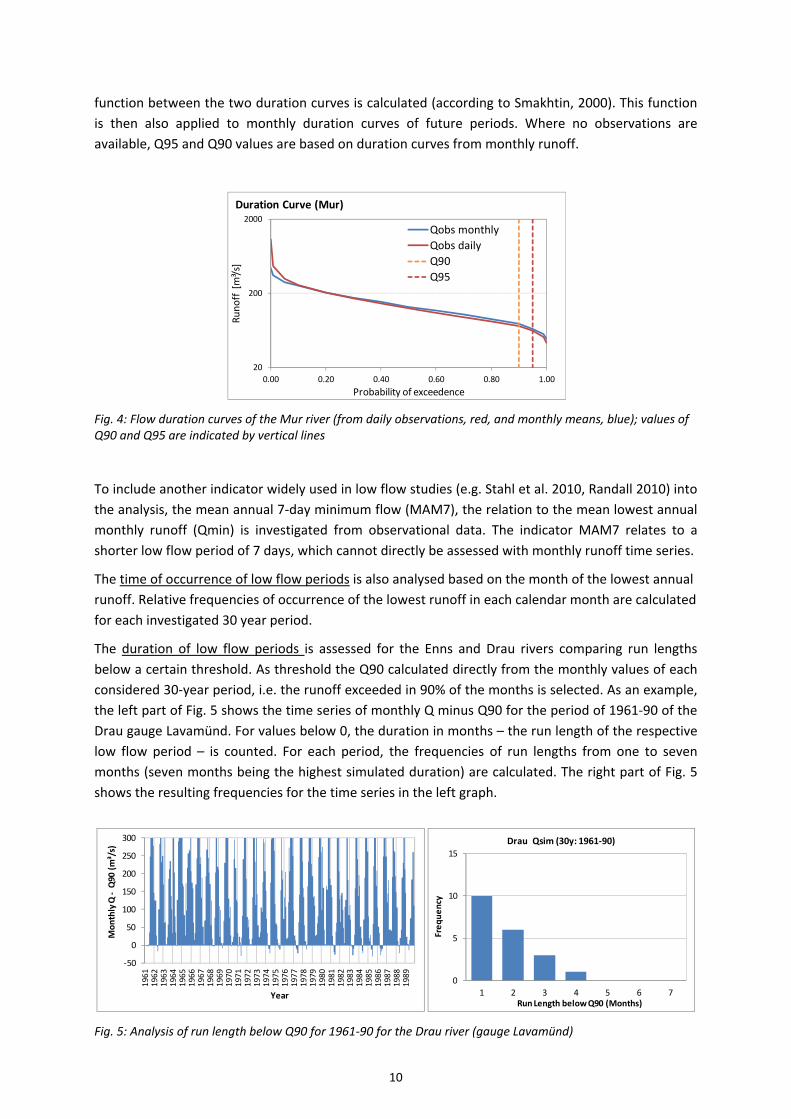
For low flow runoff, several indicators are applied: the mean lowest monthly runoff in a year (Qmin),

runoff exceeded on 95% of the days (Q95) and runoff exceeded on 90% of the days (Q90). The

derivation of Q95 and Q90 from duration curves is shown in Fig. 4. The figure also shows that there

are slight differences between the values calculated with daily runoff values and with monthly

values, especially for very high and very low runoff. Where daily observations are available, a transfer

10

function between the two duration curves is calculated (according to Smakhtin, 2000). This function

is then also applied to monthly duration curves of future periods. Where no observations are

available, Q95 and Q90 values are based on duration curves from monthly runoff.

Fig. 4: Flow duration curves of the Mur river (from daily observations, red, and monthly means, blue); values of Q90 and Q95 are indicated by vertical lines

To include another indicator widely used in low flow studies (e.g. Stahl et al. 2010, Randall 2010) into

the analysis, the mean annual 7‐day minimum flow (MAM7), the relation to the mean lowest annual

monthly runoff (Qmin) is investigated from observational data. The indicator MAM7 relates to a

shorter low flow period of 7 days, which cannot directly be assessed with monthly runoff time series.

The time of occurrence of low flow periods is also analysed based on the month of the lowest annual

runoff. Relative frequencies of occurrence of the lowest runoff in each calendar month are calculated

for each investigated 30 year period.

The duration of low flow periods is assessed for the Enns and Drau rivers comparing run lengths

below a certain threshold. As threshold the Q90 calculated directly from the monthly values of each

considered 30‐year period, i.e. the runoff exceeded in 90% of the months is selected. As an example,

the left part of Fig. 5 shows the time series of monthly Q minus Q90 for the period of 1961‐90 of the

Drau gauge Lavamünd. For values below 0, the duration in months – the run length of the respective

low flow period – is counted. For each period, the frequencies of run lengths from one to seven

months (seven months being the highest simulated duration) are calculated. The right part of Fig. 5

shows the resulting frequencies for the time series in the left graph.

Fig. 5: Analysis of run length below Q90 for 1961‐90 for the Drau river (gauge Lavamünd)

20

200

2000

0.00 0.20 0.40 0.60 0.80 1.00

Runoff [m³/s]

Probability of exceedence

Duration Curve (Mur)

Qobs monthly

Qobs daily

Q90

Q95

‐50

0

50

100

150

200

250

300

1961

1962

1963

1964

1965

1966

1967

1968

1969

1970

1971

1972

1973

1974

1975

1976

1977

1978

1979

1980

1981

1982

1983

1984

1985

1986

1987

1988

1989

Monthly Q ‐Q90 (m³/s)

Year

0

5

10

15

1 2 3 4 5 6 7

Frequency

Run Length below Q90 (Months)

Drau Qsim (30y: 1961‐90)

11

For comparison of different periods and scenarios a measure of the skewness of the run length

distribution is calculated according to Peel et al. 2004:

∑,

with ai being the frequency of run length bi, j the longest observed run length and N the number of

observed months.

2.3.2. Long‐term persistence and periodicity

Time series of runoff with 21st century scenario input data appear to show longer and more

pronounced cyclic fluctuations than observed time series of the 20th century when evaluated visually.

A systematic investigation of this effect is carried out exemplarily for two large Austrian rivers, the

Enns in the central northern Alps and the Drau, covering the south of Austria.

Mean annual runoff time series for the most downstream gauge are aggregated from observations,

simulations with observed input data and scenario simulations. Three 48‐year periods are compared:

1952‐1999, 2002‐2049 and 2043‐2090. Linear trends in each 48‐year time series are removed before

the analysis. The comparison of runoff observations and simulations with observed input data is

conducted for an upstream gauge for the Drau, where such a long observation is available, and for a

shorter period of 35 years for the Enns.

Long‐term persistence and fluctuations in the data is analysed with the run length below median (cf.

Peel et al. 2004, see also previous section on duration of low flow periods. For the calculation of this

value, the time series is divided into years above and below the long term median (as shown

exemplarily for the Enns in Fig. 6, left). The length of consecutive years – the run length – below the

median is counted. The resulting distribution of different run lengths is plotted, as in Fig. 6 right. The

5‐year run, for example, refers to the period of 1982 to 1986. As for monthly runoff below Q90, a

skewness measure g is calculated (according to Peel et al. 2004) for the run length distribution. Here,

N denominates the number of years.

Fig. 6: Example of the distribution of run length below the median (right) for a 35 year time series of the Enns (left).

Long‐term periodicity in the runoff time series was also assessed analyzing autocorrelation patterns

for different lags (cf. Pekárová et al. 2003). Autocorrelation plots are generated for lags of up to N/2.

Values of autocorrelation coefficients and their sequences are analysed visually.

‐80

‐60

‐40

‐20

0

20

40

60

80

1965

1967

1969

1971

1973

1975

1977

1979

1981

1983

1985

1987

1989

1991

1993

1995

1997

1999

Mean

annual Q

‐Median Q

(m³/s)

Year

0

1

2

3

4

5

6

7

8

9

10

1 2 3 4 5 6 7 8 9 10

Frequency

Run Length below the Median (Years)

Enns Qobs (35y:1965‐1999)

12

For the REMO‐UBA model, results with emission scenarios A1B and A2 were compared. For this

model, no control run is available, so results from scenario simulations are compared with results

from hydrological simulations using observations as input data. These analyses are carried out for

both, Enns and Drau river in order to assess regional differences.

For the models Aladin‐Arpege and RegCM3, hydrological simulation with control run data as input

can be used. For these models, scenario simulations are compared with control run simulations, in

order to assess, if climate model data generally leads to different persistence and cyclicity behavior

in the hydrological time series or if trends are due to climate change.

2.4. Impact of climate change on alpine reservoirs

For the catchment areas of three selected alpine reservoirs changes in the long term means of

relevant water balance components are analysed. The development of runoff and precipitation in

general, but also portions of snow and rain precipitation, snow accumulation and snow melt and the

contributions of snow melt and glacier melt to runoff are considered. The analyses are mostly based

on water balance simulations driven by REMO‐UBA A1B input data, with some comparison to results

with different emission scenarios (A2, B1) and different models (Aladin‐Arpege, RegCM3). Only local

runoff and precipitation in the alpine catchment areas is included.

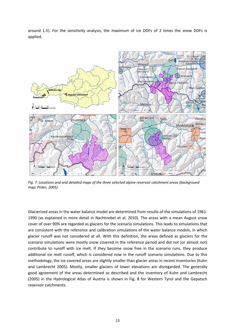
The location of the selected catchment areas is shown in Fig. 7, top left. The other maps in Fig. 7

show the catchment areas and the respective 1x1km elements of the water balance model.

The Gepatsch reservoir is located in the Kaunertal in Tyrol, damming the Fraggenbach or Fragge.

Water is also diverted from the adjacent catchments of the Pitze, of some smaller Inn tributaries and

some downstream Fragge tributaries (Fig. 7, bottom left). The areas in the water balance model that

are considered to be part of these catchments sum up to 286 km², with a glacierized area of 51 km²

(in 2000). The mean elevation is 2636 m a.s.l.

Also in Tyrol, the catchment areas of the Sellrain‐Silz area are dammed mainly in the Finstertal

reservoir and contribute to hydropower production of the Kühtai power plant. Water of several

tributaries of the Ötztaler Ache and the Inn is diverted to the reservoir (Fig. 7, bottom right). Of the

catchment areas of 138 km² in the water balance model, 18 km² are glacierized (in 2000). The mean

elevation in the catchments is 2530 m a.s.l.

Information about the catchment areas of the hydropower plant systems of Gepatsch/Kaunertal and

Sellrain‐Silz was provided by TIWAG.

The catchment areas of the Uttendorf and Kaprun reservoirs and hydropower plants are located in

Salzburg and Carinthia. Water from headwater basins of tributaries of the Salzach and Drau are

diverted to several alpine reservoirs (Fig. 7, top right). The catchment areas considered in this

analysis sum up to 192 km², with 36 km² of glaciers, and a mean elevation of 2571 m a.s.l.

For the Gepatsch reservoir, a detailed investigation of the development of the glaciers in the

catchment areas is conducted. In this context, the sensitivity of simulated glacier melt to the

selection of day‐degree‐factors (DDFs) for ice is assessed. In the original simulations with the simple

glacier melt model, the same day‐degree‐factors were assigned for snow and ice. Their values are

based on values determined by Kling (2006) for snow. Ice DDfs might, however, be higher than snow

DDFs due to the darker surface (and therefore reduced albedo) of glaciers. Based on publications by

Maniak (2010) , Nolin et al. (2010) and Kayastha et al. (2003) it is concluded, that values for ice DDFs

are in the range of 1 to maximum 2 times snow DDFs (most of the values in the cited literature are

13

around 1.5). For the sensitivity analysis, the maximum of ice DDFs of 2 times the snow DDFs is

applied.

Fig. 7: Locations and and detailed maps of the three selected alpine reservoir catchment areas (background map: Pirker, 2005)

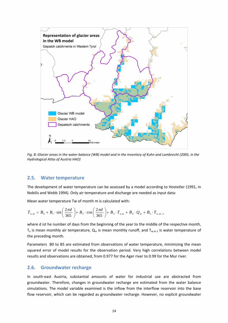
Glacierized areas in the water balance model are determined from results of the simulations of 1961‐

1990 (as explained in more detail in Nachtnebel et al. 2010). The areas with a mean August snow

cover of over 90% are regarded as glaciers for the scenario simulations. This leads to simulations that

are consistent with the reference and calibration simulations of the water balance models, in which

glacier runoff was not considered at all. With this definition, the areas defined as glaciers for the

scenario simulations were mostly snow covered in the reference period and did not (or almost not)

contribute to runoff with ice melt. If they become snow free in the scenario runs, they produce

additional ice melt runoff, which is considered now in the runoff scenario simulations. Due to this

methodology, the ice covered areas are slightly smaller than glacier areas in recent inventories (Kuhn

and Lambrecht 2005). Mostly, smaller glaciers of lower elevations are disregarded. The generally

good agreement of the areas determined as described and the inventory of Kuhn and Lambrecht

(2005) in the Hydrological Atlas of Austria is shown in Fig. 8 for Western Tyrol and the Gepatsch

reservoir catchments.

Gepatsch reservoir / Kaunertal Finstertal reservoir / Sellrain Silz

Kaprun Uttendorf

14

Fig. 8: Glacier areas in the water balance (WB) model and in the inventory of Kuhn and Lambrecht (2005, in the Hydrological Atlas of Austria HAO)

2.5. Water temperature

The development of water temperature can be assessed by a model according to Hostetler (1991, in

Nobilis and Webb 1994). Only air temperature and discharge are needed as input data:

Mean water temperature Tw of month m is calculated with:

1,54,3210, 365

2cos

365

2sin

mwmmamw TBQBTB

dB

dBBT

where d ist he number of days from the beginning of the year to the middle of the respective month,

Ta is mean monthly air temperature, Qm is mean monthly runoff, and Tw,m‐1 is water temperature of

the preceding month.

Parameters B0 to B5 are estimated from observations of water temperature, minimizing the mean

squared error of model results for the observation period. Very high correlations between model

results and observations are obtained, from 0.977 for the Ager river to 0.99 for the Mur river.

2.6. Groundwater recharge

In south‐east Austria, substantial amounts of water for industrial use are abstracted from

groundwater. Therefore, changes in groundwater recharge are estimated from the water balance

simulations. The model variable examined is the inflow from the interflow reservoir into the base

flow reservoir, which can be regarded as groundwater recharge. However, no explicit groundwater

15

model is applied, and groundwater flow over borders of subbasins in the water balance model is not

considered. The results therefore refer only to local groundwater recharge. Groundwater bodies in

connection with larger rivers, as in the downstream Mur basin, are influenced by both, surface and

groundwater inflow from upstream. Further analysis of effects of changes in groundwater availability

for water abstraction in such regions should combine information about changes in local

groundwater recharge and in river runoff.

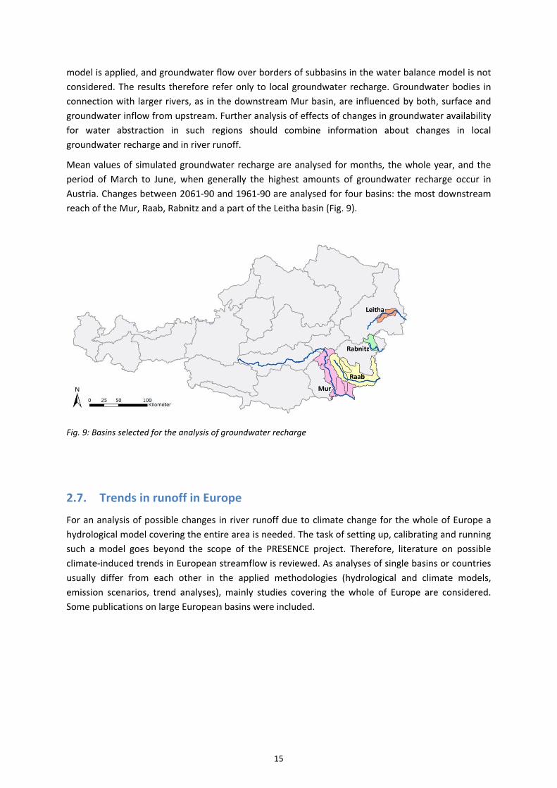
Mean values of simulated groundwater recharge are analysed for months, the whole year, and the

period of March to June, when generally the highest amounts of groundwater recharge occur in

Austria. Changes between 2061‐90 and 1961‐90 are analysed for four basins: the most downstream

reach of the Mur, Raab, Rabnitz and a part of the Leitha basin (Fig. 9).

Fig. 9: Basins selected for the analysis of groundwater recharge

2.7. Trends in runoff in Europe

For an analysis of possible changes in river runoff due to climate change for the whole of Europe a

hydrological model covering the entire area is needed. The task of setting up, calibrating and running

such a model goes beyond the scope of the PRESENCE project. Therefore, literature on possible

climate‐induced trends in European streamflow is reviewed. As analyses of single basins or countries

usually differ from each other in the applied methodologies (hydrological and climate models,

emission scenarios, trend analyses), mainly studies covering the whole of Europe are considered.

Some publications on large European basins were included.

16

3. Input data

For PRESENCE, data of three regional climate models (RCMs) published in the ENSEMBLES project

(van der Linden and Mitchell 2009) are selected, downloaded, corrected and prepared for the use in

impact assessment by the Institute of Meteorology (BOKUMET). For the hydrological application, the

variables temperature and precipitation are used. The three selected models are RegCM3 by ICTP

(driving General Circulation Model – GCM – ECHAM5), Aladin‐Arpege by CNRM (the RCM Aladin

driven by the GCM Arpege) and REMO by MPI (driving GCM ECHAM5). In the new water balance

simulations in the framework of PREENCE, only the two models RegCM3 and Aladin‐Arpege are

applied. REMO results from the 25km ENSEMBLES version of this model are supposed to be rather

similar to the results from the 10km REMO‐UBA version, that has been successfully applied in the

preceding KlimAdapt project. Therefore, the results with REMO‐UBA are used together with new

simulation results with RegCM3 and Aladin‐Arpege for further and more detailed analysis of climate

change impacts on hydrology.

3.1. Corrections of RCM data

The selected ENSEMBLES models are corrected with a quantile mapping approach (cf. Déqué 2007)

using large scale 25x25km observation fields for temperature (E‐OBS, Haylock et al. 2008) and

precipitation (Frei and Schär 1998) as reference observations. The reference period for this

correction is 1971‐1999 for precipitation and 1971‐2000 for temperature.

It is known that local and regional distributions of the variables temperature and precipitation in the

large scale observation data set do not correspond well with local observations and that therefore

RCM data corrected based only on these data are not suitable for hydrological applications (Senoner

et al. 2011). Therefore, a 1x1km climatology for 1961‐1990 of temperature and precipitation that has

been developed at the IWHW especially for water balance modeling in Austria (Fürst et al. 2007), is

used as second reference in a further correction step. After preliminary application by the

meteorologists, the values for the catchment area of the Erlauf river (subbasin 09_15 in the water

balance model) were replaced by the values in the very similar climatology of Kling et al. 2005. While

the quantile mapping correction is conducted with daily data, the second correction is applied for

monthly data only. The differences between the long term monthly mean values of the large scale

observation data set (E‐OBS for temperature and Frei/Schär for precipitation) and the IWHW

observation data set is calculated for each 1x1km pixel. These mean monthly deviations are then

applied as correction factors to the RCM data that was corrected with the large scale observations.

Due to different reference periods (1971‐1999/2000 for the 25km data and 1961‐1990 for the IWHW

1km data), the resulting means of the reference period of the hydrological simulation, 1961‐1990,

deviate slightly from the original IWHW data (see chapter 4.1.2).

3.2. Climate change signals

The following graphs (Fig. 10 to Fig. 13) show climate change signals of mean annual temperature

and precipitation of the two PRESENCE climate models for the periods of 2051‐2080 and 2061‐2090,

both compared to 1961‐1990.

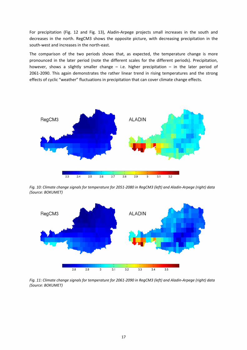
Generally, Aladin‐Arpege projects higher temperature increases (Fig. 10 and Fig. 11). The models

coincide projecting a more pronounced rise in temperature for alpine areas.

17

For precipitation (Fig. 12 and Fig. 13), Aladin‐Arpege projects small increases in the south and

decreases in the north. RegCM3 shows the opposite picture, with decreasing precipitation in the

south‐west and increases in the north‐east.

The comparison of the two periods shows that, as expected, the temperature change is more

pronounced in the later period (note the different scales for the different periods). Precipitation,

however, shows a slightly smaller change – i.e. higher precipitation – in the later period of

2061‐2090. This again demonstrates the rather linear trend in rising temperatures and the strong

effects of cyclic “weather” fluctuations in precipitation that can cover climate change effects.

Fig. 10: Climate change signals for temperature for 2051‐2080 in RegCM3 (left) and Aladin‐Arpege (right) data (Source: BOKUMET)

Fig. 11: Climate change signals for temperature for 2061‐2090 in RegCM3 (left) and Aladin‐Arpege (right) data (Source: BOKUMET)

18

Fig. 12: Climate change signals for precipitation for 2051‐2080 in RegCM3 (left) and Aladin‐Arpege (right) data (Source: BOKUMET)

Fig. 13: Climate change signals for precipitation for 2061‐2090 in RegCM3 (left) and Aladin‐Arpege (right) data (Source: BOKUMET)

19

4. Results

4.1. Performance of the water balance model

4.1.1. Simulations with observed input data

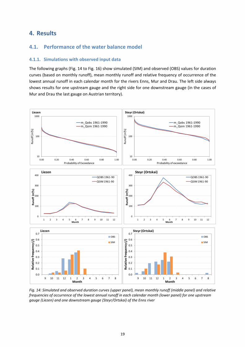
The following graphs (Fig. 14 to Fig. 16) show simulated (SIM) and observed (OBS) values for duration

curves (based on monthly runoff), mean monthly runoff and relative frequency of occurrence of the

lowest annual runoff in each calendar month for the rivers Enns, Mur and Drau. The left side always

shows results for one upstream gauge and the right side for one downstream gauge (in the cases of

Mur and Drau the last gauge on Austrian territory).

Fig. 14: Simulated and observed duration curves (upper panel), mean monthly runoff (middle panel) and relative frequencies of occurrence of the lowest annual runoff in each calendar month (lower panel) for one upstream gauge (Liezen) and one downstream gauge (Steyr/Ortskai) of the Enns river

10

100

1000

0.00 0.20 0.40 0.60 0.80 1.00

Runoff [m

³/s]

Probability of Exceedance

Liezen

m_Qobs 1961‐1990m_Qsim 1961‐1990

10

100

1000

0.00 0.20 0.40 0.60 0.80 1.00

Runoff [m

³/s]

Probability of exceedance

Steyr (Ortskai)

m_Qobs 1961‐1990m_Qsim 1961‐1990

0

100

200

300

400

1 2 3 4 5 6 7 8 9 10 11 12

Runoff (m³/s)

Month

Liezen

QOBS 1961‐90

QSIM 1961‐90

0

100

200

300

400

1 2 3 4 5 6 7 8 9 10 11 12

Runoff (m³/s)

Month

Steyr (Ortskai)

QOBS 1961‐90

QSIM 1961‐90

0.0

0.1

0.2

0.3

0.4

0.5

0.6

0.7

9 10 11 12 1 2 3 4 5 6 7 8

Relative frequency (/)

Month

Liezen

OBS

SIM

0.0

0.1

0.2

0.3

0.4

0.5

0.6

0.7

9 10 11 12 1 2 3 4 5 6 7 8


Month

Steyr (Ortskai)

OBS

SIM

20

The simulated duration curves show a very good agreement with duration curves from observed

discharge for all six gauges. The overall distribution of runoff is therefore simulated very well. In the

range of the lowest values some very small deviations appear.

The seasonal distribution of runoff is also simulated very well, but there are higher discrepancies

between simulations and observations. For Drau and Mur rivers, the simulations show slight

overestimations of simulated mean monthly runoff in spring and summer and a slight

underestimation in fall and winter. For the Enns, mean runoff in spring and winter is simulated

accurately, in summer, simulations are too low, and in fall slightly too high.

Fig. 15: Simulated and observed duration curves (upper panel), mean monthly runoff (middle panel) and relative frequencies of occurrence of the lowest annual runoff in each calendar month (lower panel) for one upstream gauge (Gestüthof) and one downstream gauge (Mureck/Spielfeld) of the Mur river

1

10

100

1000

0.00 0.20 0.40 0.60 0.80 1.00

Runoff [m

³/s]


Gestüthof

m_Qobs 1961‐1990m_Qsim 1961‐1990

10

100

1000

0.00 0.20 0.40 0.60 0.80 1.00

Runoff [m

³/s]


Mureck/Spielfeld

m_Qobs 1974‐2000m_Qsim 1961‐1990

0

100

200

300

1 2 3 4 5 6 7 8 9 10 11 12

Runoff (m³/s)

Month

Gestüthof

QOBS 1961‐90

QSIM 1961‐90

0

100

200

300

1 2 3 4 5 6 7 8 9 10 11 12

Runoff (m³/s)

Month

Mureck/Spielfeld

QOBS 1961‐90

QSIM 1961‐90

0.0

0.1

0.2

0.3

0.4

0.5

0.6

0.7

0.8

9 10 11 12 1 2 3 4 5 6 7 8


Month

Gestüthof

OBS

SIM

0.0

0.1

0.2

0.3

0.4

0.5

0.6

0.7

0.8

9 10 11 12 1 2 3 4 5 6 7 8


Month

Mureck/Spielfeld

OBS

SIM

21

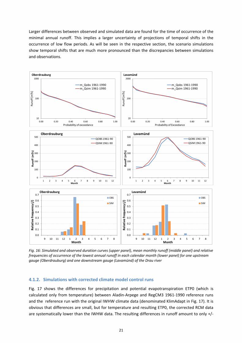
Larger differences between observed and simulated data are found for the time of occurrence of the

minimal annual runoff. This implies a larger uncertainty of projections of temporal shifts in the

occurrence of low flow periods. As will be seen in the respective section, the scenario simulations

show temporal shifts that are much more pronounced than the discrepancies between simulations

and observations.

Fig. 16: Simulated and observed duration curves (upper panel), mean monthly runoff (middle panel) and relative frequencies of occurrence of the lowest annual runoff in each calendar month (lower panel) for one upstream gauge (Oberdrauburg) and one downstream gauge (Lavamünd) of the Drau river

4.1.2. Simulations with corrected climate model control runs

Fig. 17 shows the differences for precipitation and potential evapotranspiration ETP0 (which is

calculated only from temperature) between Aladin‐Arpege and RegCM3 1961‐1990 reference runs

and the reference run with the original IWHW climate data (denominated KlimAdapt in Fig. 17). It is

obvious that differences are small, but for temperature and resulting ETP0, the corrected RCM data

are systematically lower than the IWHW data. The resulting differences in runoff amount to only +/‐

10

100

1000

0.00 0.20 0.40 0.60 0.80 1.00

Runoff [m

³/s]


Oberdrauburg

m_Qobs 1961‐1990m_Qsim 1961‐1990

20

200

2000

0.00 0.20 0.40 0.60 0.80 1.00Runoff [m

³/s]

Probability of Exceedance

Lavamünd

m_Qobs 1961‐1990m_Qsim 1961‐1990

0

100

200

300

400

500

1 2 3 4 5 6 7 8 9 10 11 12

Runoff (m³/s)

Month

Oberdrauburg

QOBS 1961‐90

QSIM 1961‐90

0

100

200

300

400

500

1 2 3 4 5 6 7 8 9 10 11 12

Runoff (m³/s)

Month

Lavamünd

QOBS 1961‐90

QSIM 1961‐90

0.0

0.1

0.2

0.3

0.4

0.5

0.6

0.7

9 10 11 12 1 2 3 4 5 6 7 8


Month

Oberdrauburg

OBS

SIM

0.0

0.1

0.2

0.3

0.4

0.5

0.6

0.7

9 10 11 12 1 2 3 4 5 6 7 8


Month

Lavamünd

OBS

SIM

22

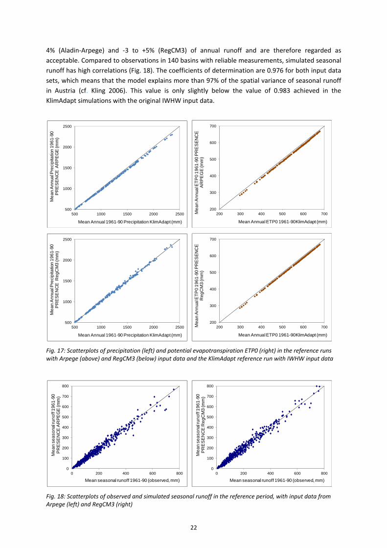
4% (Aladin‐Arpege) and ‐3 to +5% (RegCM3) of annual runoff and are therefore regarded as

acceptable. Compared to observations in 140 basins with reliable measurements, simulated seasonal

runoff has high correlations (Fig. 18). The coefficients of determination are 0.976 for both input data

sets, which means that the model explains more than 97% of the spatial variance of seasonal runoff

in Austria (cf. Kling 2006). This value is only slightly below the value of 0.983 achieved in the

KlimAdapt simulations with the original IWHW input data.

Fig. 17: Scatterplots of precipitation (left) and potential evapotranspiration ETP0 (right) in the reference runs with Arpege (above) and RegCM3 (below) input data and the KlimAdapt reference run with IWHW input data

Fig. 18: Scatterplots of observed and simulated seasonal runoff in the reference period, with input data from Arpege (left) and RegCM3 (right)

500

1000

1500

2000

2500

500 1000 1500 2000 2500

Me

an

An

nua

l Pre

cip

itatio

n 1

96

1-9

0

PR

ES

EN

CE

AR

PE

GE

(mm

)

Mean Annual 1961-90 Precipitation KlimAdapt (mm)

200

300

400

500

600

700

200 300 400 500 600 700Me

an

An

nua

l ET

P0

19

61

-90

PR

ES

EN

CE

A

RP

EG

E (m

m)

Mean Annual ETP0 1961-90KlimAdapt (mm)

500

1000

1500

2000

2500

500 1000 1500 2000 2500

Me

an

An

nua

l Pre

cip

itatio

n 1

96

1-9

0

PR

ES

EN

CE

Re

gC

M3

(mm

)

Mean Annual 1961-90 Precipitation KlimAdapt (mm)

200

300

400

500

600

700

200 300 400 500 600 700Me

an

An

nua

l ET

P0

19

61

-90

PR

ES

EN

CE

R

eg

CM

3 (m

m)

Mean Annual ETP0 1961-90KlimAdapt (mm)

0

100

200

300

400

500

600

700

800

0 200 400 600 800

Me

an

se

aso

nal r

un

off

19

61

-90

P

RE

SE

NC

E A

RP

EG

E (m

m)

Mean seasonal runoff 1961-90 (observed, mm)

0

100

200

300

400

500

600

700

800

0 200 400 600 800

Me

an

se

aso

nal r

un

off

19

61

-90

P

RE

SE

NC

E R

eg

CM

3 (m

m)

Mean seasonal runoff 1961-90 (observed, mm)

23

4.2. Runoff elasticity

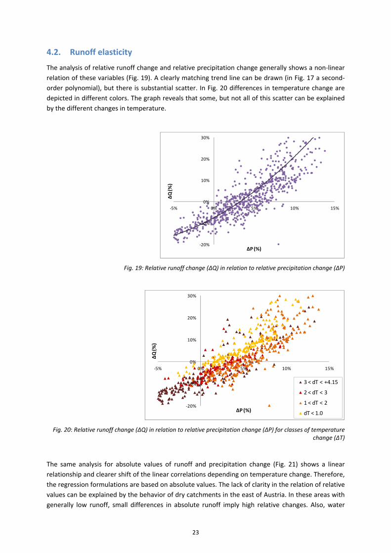
The analysis of relative runoff change and relative precipitation change generally shows a non‐linear

relation of these variables (Fig. 19). A clearly matching trend line can be drawn (in Fig. 17 a second‐

order polynomial), but there is substantial scatter. In Fig. 20 differences in temperature change are

depicted in different colors. The graph reveals that some, but not all of this scatter can be explained

by the different changes in temperature.

Fig. 19: Relative runoff change (ΔQ) in relation to relative precipitation change (ΔP)

Fig. 20: Relative runoff change (ΔQ) in relation to relative precipitation change (ΔP) for classes of temperature change (ΔT)

The same analysis for absolute values of runoff and precipitation change (Fig. 21) shows a linear

relationship and clearer shift of the linear correlations depending on temperature change. Therefore,

the regression formulations are based on absolute values. The lack of clarity in the relation of relative

values can be explained by the behavior of dry catchments in the east of Austria. In these areas with

generally low runoff, small differences in absolute runoff imply high relative changes. Also, water

‐20%

‐10%

0%

10%

20%

30%

‐5% 0% 5% 10% 15%

ΔQ (%

)

ΔP (%)

‐20%

‐10%

0%

10%

20%

30%

‐5% 0% 5% 10% 15%

ΔQ (%

)

ΔP (%)

3 < dT < +4.15

2 < dT < 3

1 < dT < 2

dT < 1.0

24

balance simulations have higher uncertainties in these catchments, which can lead to slightly

different results due to similar precipitation and temperature changes (which then mean high

relative differences).

Fig. 21: Absolute runoff change (ΔQ) in relation to absolute precipitation change (ΔP) for classes of temperature change (ΔT)

A multiple linear regression with ΔQ as dependent variable and ΔP and ΔT as explanatory variables is

carried out including all values (9 cases: 3 periods for each of the 3 scenarios) in all 188 Austrian

catchments. The regression yields a high coefficient of determination of 0.91 with the following

equation:

∆ 0.9893 ∙ ∆ 1.8400 ∙ ∆ 0.0456

Fig. 22 shows a scatter plot with the original results of runoff change ΔQ of the water balance model

and the results from this regression model based on the simulation data. There is a generally good

agreement, with larger deviations for lower runoff. Including mean catchment elevation as additional

explanatory variable leads to no significant improvement, with a coefficient of determination of 0.92.

Fig. 22: Comparison of results for absolute runoff change (ΔQ) with the water balance model and the regression model based on precipitation and temperature change

‐20

‐15

‐10

‐5

0

5

10

15

20

‐10 ‐5 0 5 10 15 20ΔQ (m

m)

ΔP (mm)

3 < dT < +4.15

2 < dT < 3

1 < dT < 2

dT < 1.0

‐25

‐20

‐15

‐10

‐5

‐

5

10

15

20

25

‐25 ‐20 ‐15 ‐10 ‐5 ‐ 5 10 15 20 25

∆Q (m

m) water balance model

ΔQ (mm) regression model

Austria (188 catchments)

25

As the highest deviations of the regression model for all Austrian catchments occur for eastern

lowland catchments, the procedure is rerun for alpine catchments and lowland catchments

separately. The total 188 catchments are grouped into 107 alpine catchments and 81 lowland

catchments, as shown in Fig. 23. The division is based on the main river basins in the water balance

model, which leads to the inclusion of some partially alpine catchments (as for example the Ybbs and

Traisen catchments) into the lowland part and vice versa (as for example the Ager catchment).

Alpine runoff elasticity can be explained with the following equation, yielding a very high coefficient

of determination of 0.97:

∆ 1.0264 ∙ ∆ 2.2641 ∙ ∆ 0.0377

Lowland runoff elasticity is explained with a lower coefficient of determination of 0.86 by:

∆ 0.8055 ∙ ∆ 1.0067 ∙ ∆ 0.4955

The scatter plots in Fig. 24 shows a better fit along the range of change values in both areas. The

remaining overestimated ΔQ values around ‐10mm of the regression model are all results for

catchments in the South of Austria. This suggests that a more detailed regional division could further

improve the performance of the regression model based on ΔP and ΔT.

Fig. 23: Division into alpine and lowland catchments

Fig. 24: Comparison of results for ΔQ with the water balance model and the regression models for alpine and lowland catchments

‐25

‐20

‐15

‐10

‐5

‐

5

10

15

20

25

‐25 ‐20 ‐15 ‐10 ‐5 ‐ 5 10 15 20 25

ΔQ (m

m) water balan

ce model


Alpine (107 catchments)

‐25

‐20

‐15

‐10

‐5

‐

5

10

15

20

25

‐25 ‐20 ‐15 ‐10 ‐5 ‐ 5 10 15 20 25

ΔQ (m

m) water balan

ce model


Lowland (81 catchments)

26

4.3. Spatial patterns of change in local runoff

The maps in Fig. 25 show the relative change in mean annual runoff of each of the 188 basins of the

water balance model for the period of 2051‐2080, relative to the mean of 1961‐1990, simulated with

Aladin‐Arpege and RegCM3 model data.

Fig. 25: Change in mean annual runoff 2051‐2080 relative to 1961‐1990, simulated with Aladin‐Arpege (top) and RegCM3 (bottom) input data

27

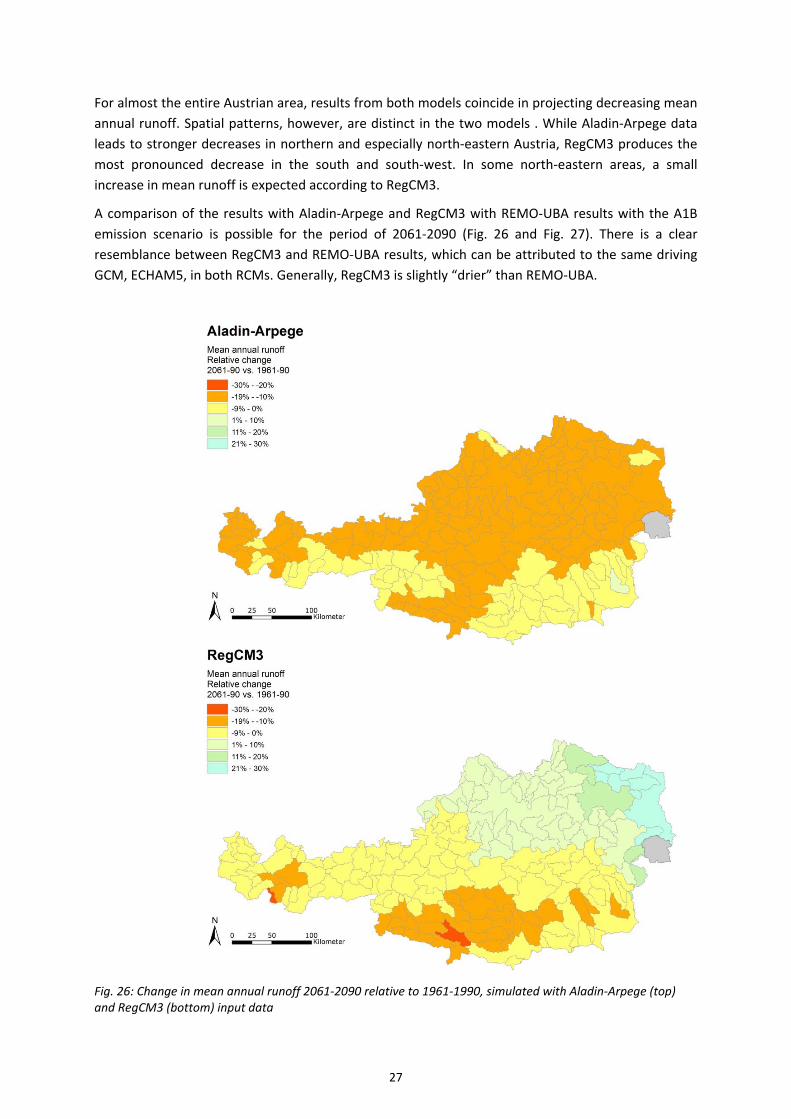
For almost the entire Austrian area, results from both models coincide in projecting decreasing mean

annual runoff. Spatial patterns, however, are distinct in the two models . While Aladin‐Arpege data

leads to stronger decreases in northern and especially north‐eastern Austria, RegCM3 produces the

most pronounced decrease in the south and south‐west. In some north‐eastern areas, a small

increase in mean runoff is expected according to RegCM3.

A comparison of the results with Aladin‐Arpege and RegCM3 with REMO‐UBA results with the A1B

emission scenario is possible for the period of 2061‐2090 (Fig. 26 and Fig. 27). There is a clear

resemblance between RegCM3 and REMO‐UBA results, which can be attributed to the same driving

GCM, ECHAM5, in both RCMs. Generally, RegCM3 is slightly “drier” than REMO‐UBA.

Fig. 26: Change in mean annual runoff 2061‐2090 relative to 1961‐1990, simulated with Aladin‐Arpege (top) and RegCM3 (bottom) input data

28

Comparing the maps of Aladin‐Arpege and RegCM3 in Fig. 25 and Fig. 26 reveals that the spatial

patterns of the mean change of each model is very similar for these two rather close periods, but the

general level of mean runoff is higher in the later period in both models. This means that

precipitation is considerably higher in the period of 2061‐2090 than in 2051‐2080, as temperature

and therefore evapotranspiration are also higher in the later period. This again underlines the

importance of keeping in mind that precipitation in climate model data – like observed precipitation

– shows cyclic fluctuations and that therefore the selection of the periods for comparison has a

relevant effect on the results.

Fig. 27: Change in mean annual runoff 2061‐2090 relative to 1961‐1990, simulated with REMO‐UBA (from Kranzl et al. 2010)

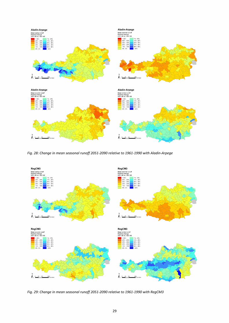
Spatial patterns in seasonal runoff resulting from Aladin‐Arpege and RegCM3 are more similar to

each other (Fig. 28 and Fig. 29). Also the results of the two periods 2051‐2080 and 2061‐2090 are

very similar (and the graphs for 2061‐2090 are not shown therefore). The clearest differences can be

found for autumn and winter, for which RegCM3 shows generally higher runoff than Aladin‐Arpege.

The seasonal runoff maps of REMO‐UBA (not reproduced here) closely resemble those of RegCM3,

with a slightly wetter autumn in the RegCM3 results.

29

Fig. 28: Change in mean seasonal runoff 2051‐2090 relative to 1961‐1990 with Aladin‐Arpege

Fig. 29: Change in mean seasonal runoff 2051‐2090 relative to 1961‐1990 with RegCM3

30

4.4. Changes in river runoff

4.4.1. Mean runoff

Results for mean flow conditions under climate change depend on the climate model and the

emission scenario. Fig. 30 shows the development of the simulated mean discharge MQsim for all

considered gauges along the three rivers Enns, Mur and Drau (from upstream, left, to

downstream,right) based on REMO‐UBA data. The mean value of the period 1961‐1990 is regarded

as reference value for each gauge and has the value 1.

Fig. 30: Development of simulated mean flow (MQsim) through 30‐year periods around 1975, 2025, 2050, and

2075 for Enns (top), Mur (middle) and Drau (bottom) with the REMO‐UBA scenarios A1B (left) and A2 (right)

The simulated changes are generally in the range of +/‐ 10%. In the second half of the 21st century

simulated discharges tend to be lower in the generally “drier” A1B scenario (left column in Fig. 30)

than in the “wetter” A2 scenario (right column in Fig. 30). Both scenarios, however, show a negative

0.8

0.9

1

1.1

1.2

Schladming Liezen (Röthelbrücke)

KW Schönau / SB 8_6

Steyr (Ortskai)

Enns ‐ A1B

MQsim 1961‐90 MQsim 2011‐40 MQsim 2036‐65 MQsim 2061‐90

0.8

0.9

1

1.1

1.2



Steyr (Ortskai)

Enns ‐ A2


0.8

0.9

1

1.1

1.2

St.Michael i. Lg. (Mur)

Gestüthof St.Georgen ob

Judenburg

Leoben Bruck an der Mur

unter Mürz

Friesach Mureck / Spielfeld

Mur ‐ A1B


0.8

0.9

1

1.1

1.2



Judenburg


unter Mürz


Mur ‐ A2


0.8

0.9

1

1.1

1.2

Rabland Oberdrauburg Sachsenburg (Brücke)

Villach Lavamünd

Drau ‐ A1B


0.8

0.9

1

1.1

1.2


Villach Lavamünd

Drau ‐ A2


31

trend in mean runoff within the 21st century for almost all considered gauges. In the A2 scenario,

mean runoff around 2075 is still higher than around 1975, for Enns and Mur. For the entire Austrian

Drau basin (analysed at the last gauge in Lavamünd), mean runoff around 2075 is lower than around

1975 in both scenarios. In all three rivers, results for mean flow are very similar for all considered

gauges.

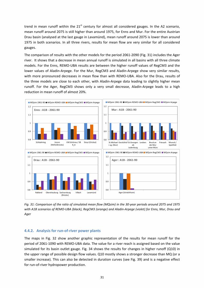
The comparison of results with the other models for the period 2061‐2090 (Fig. 31) includes the Ager

river. It shows that a decrease in mean annual runoff is simulated in all basins with all three climate

models. For the Enns, REMO‐UBA results are between the higher runoff values of RegCM3 and the

lower values of Aladin‐Arpege. For the Mur, RegCM3 and Aladin‐Arpege show very similar results,

with more pronounced decreases in mean flow than with REMO‐UBA. Also for the Drau, results of

the three models are close to each other, with Aladin‐Arpege data leading to slightly higher mean

runoff. For the Ager, RegCM3 shows only a very small decrease, Aladin‐Arpege leads to a high

reduction in mean runoff of almost 20%.

Fig. 31: Comparison of the ratio of simulated mean flow (MQsim) in the 30‐year periods around 2075 and 1975

with A1B scenarios of REMO‐UBA (black), RegCM3 (orange) and Aladin‐Arpege (violet) for Enns, Mur, Drau and

Ager

4.4.2. Analysis for run‐of‐river power plants

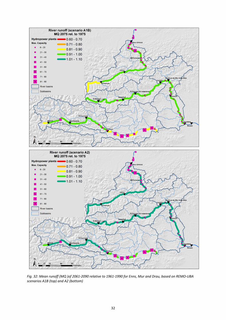
The maps in Fig. 32 show another graphic representation of the results for mean runoff for the

period of 2061‐1090 with REMO‐UBA data. The value for a river reach is assigned based on the value

simulated for its basin outlet gauge. Fig. 34 shows the results for changes in higher runoff (Q10) in

the upper range of possible design flow values. Q10 mostly shows a stronger decrease than MQ (or a

smaller increase). This can also be detected in duration curves (see Fig. 39) and is a negative effect

for run‐of‐river hydropower production.

0.8

0.9

1

1.1

1.2



Steyr (Ortskai)

Enns : A1B ‐ 2061‐90

MQsim 1961‐90 MQsim REMO‐UBA MQsim RegCM3 MQsim Arpege

0.8

0.9

1

1.1

1.2



Judenburg


unter Mürz


Mur : A1B ‐ 2061‐90


0.8

0.9

1

1.1

1.2


Villach Lavamünd

Drau : A1B ‐ 2061‐90


0.8

0.9

1

1.1

1.2

Ager (Schalchham)

Ager : A1B ‐ 2061‐90


32

Fig. 32: Mean runoff (MQ )of 2061‐2090 relative to 1961‐1990 for Enns, Mur and Drau, based on REMO‐UBA scenarios A1B (top) and A2 (bottom)

33

Fig. 33: Q10 of 2061‐2090 relative to 1961‐1990 for Enns, Mur and Drau, based on REMO‐UBA scenarios A1B (top) and A2 (bottom)

34

4.4.3. Runoff seasonality

For seasonal runoff, expected changes are rather independent of the climate model and scenario.

Fig. 34 again compares results with the different emission scenarios of REMO‐UBA, for the period

around 2075.

Fig. 34: Mean monthly runoff in 2061‐90 for the scenarios A1B and A2, compared to 1961‐90, for Enns, Mur and

Drau

0

100

200

300

400

1 2 3 4 5 6 7 8 9 10 11 12

Runoff (m³/s)

Month

Enns

Steyr (Ortskai) 1961‐1990

Steyr (Ortskai) 2061‐90 A1B

Steyr (Ortskai) 2061‐90 A2

Liezen 1961‐1990

Liezen 2061‐90 A1B

Liezen 2061‐90 A2

0

50

100

150

200

250

300

1 2 3 4 5 6 7 8 9 10 11 12

Runoff (m³/s)

Month

Mur

Mureck / Spielfeld 1961‐1990

Mureck / Spielfeld 2061‐90 A1B

Mureck / Spielfeld 2061‐90 A2

Gestüthof 1961‐1991

Gestüthof 2061‐90 A1B

Gestüthof 2061‐90 A2

0

100

200

300

400

500

600

1 2 3 4 5 6 7 8 9 10 11 12

Runoff (m

³/s)

Month

Drau

Lavamünd 1961‐1990

Lavamünd 2061‐90 A1B

Lavamünd 2061‐90 A2

Oberdrauburg 1961‐1990

Oberdrauburg 2061‐90 A1B

Oberdrauburg 2061‐90 A1B

35

The generally higher runoff in the A2 scenario is visible also in mean monthly flows, especially for the

Mur and Enns rivers. In both scenarios, however, a clear increase in winter and spring runoff is

simulated. Summer and fall runoff is projected to decrease, moderately in scenario A2, substantially

in scenario A1B. A one‐month shift of the peak in monthly runoff to earlier occurrence is simulated

more consistently for the upstream gauges, for the Drau river also for the downstream gauges. Peaks

in spring are caused by large snow melt contributions, which are expected to occur earlier and

decrease due to higher temperatures and less snow precipitation. The influence of these climate

change impacts is stronger with a higher relevance of snow processes for runoff generation in the

upstream reaches of the investigated alpine rivers.

These changes in runoff seasonality are also simulated by the other two models, RegCM3 and

Aladin‐Arpege. Simulated mean monthly runoff with all three models for 2061‐2090, compared to

1961‐1990, is shown for the same gauges in Fig. 35 (Enns), Fig. 36 (Mur) and Fig. 37 (Drau). For the

Enns, RegCM3 results are very close to REMO‐UBA simulations. For Mur and Drau, they are also very

similar, but RegCM3 shows a stronger decrease in summer. Scenario runoff simulated with

Aladin‐Arpege data generally exhibits less pronounced increases in winter than with the other two

models.

Fig. 35: Mean monthly runoff in 2061‐90, with REMO‐UBA (top), RegCM3 (bottom left) and Aladin‐Arpege

(bottom right), compared to 1961‐90, for two gauges of the river Enns

0

100

200

300

400

1 2 3 4 5 6 7 8 9 10 11 12

Runoff (m

³/s)

Month

Enns

Steyr (Ortskai) 1961‐1990

Steyr (Ortskai) 2061‐90 REMO‐UBA A1B

Liezen 1961‐1990

Liezen 2061‐90 REMO‐UBA A1B

0

100

200

300

400

1 2 3 4 5 6 7 8 9 10 11 12

Runoff (m³/s)

Month

Enns

Steyr (Ortskai) 1961‐1990 RegCM3

Steyr (Ortskai) 2061‐90 RegCM3

Liezen 1961‐1990 RegCM3

Liezen 2061‐90 RegCM3

0

100

200

300

400

1 2 3 4 5 6 7 8 9 10 11 12

Runoff (m³/s)

Month

Enns

Steyr (Ortskai) 1961‐1990 Arpege

Steyr (Ortskai) 2061‐90 Arpege

Liezen 1961‐1990 Arpege

Liezen 2061‐90 Arpege

36


(bottom right), compared to 1961‐90, for two gauges of the river Mur


(bottom right), compared to 1961‐90, for two gauges of the river Drau

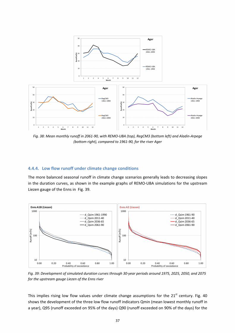
The seasonal distribution of runoff exhibits a generally different behavior on the Ager (Fig. 38), with a

less pronounced seasonality and an earlier peak, in March/April, resulting from earlier snow melt.

With all three models decreasing summer runoff is simulated with scenario data. The decrease is

strongest with Aladin‐Arpege, which again projects no increases in winter runoff and leads to a lower

peak in the beginning of the year. In the other two models, winter discharge increases. RegCM3

simulations show a lower peak in March, but no changes in April. With REMO‐UBA, the March/April

peak is projected to increase.

0

50

100

150

200

250

300

1 2 3 4 5 6 7 8 9 10 11 12

Runoff (m³/s)

Month

Mur

Mureck / Spielfeld 1961‐1990

Mureck / Spielfeld 2061‐90 REMO‐UBA A1B

Gestüthof 1961‐1991

Gestüthof 2061‐90 REMO‐UBA A1B

0

50

100

150

200

250

300

1 2 3 4 5 6 7 8 9 10 11 12

Runoff (m³/s)

Month

Mur

Mureck / Spielfeld 1961‐1990 RegCM3

Mureck / Spielfeld 2061‐90 RegCM3

Gestüthof 1961‐1991 RegCM3

Gestüthof 2061‐60 RegCM3

0

50

100

150

200

250

300

1 2 3 4 5 6 7 8 9 10 11 12Runoff (m³/s)

Month

Mur

Mureck / Spielfeld 1961‐1990 Arpege

Mureck / Spielfeld 2061‐90 Arpege

Gestüthof 1961‐1991 Arpege

Gestüthof 2061‐60 Arpege

0

100

200

300

400

500

600

1 2 3 4 5 6 7 8 9 10 11 12

Runoff (m³/s)

Month

Drau


Lavamünd 2061‐90 REMO‐UBA


Oberdrauburg 2061‐90 REMO‐UBA

0

100

200

300

400

500

600

1 2 3 4 5 6 7 8 9 10 11 12

Runoff (m³/s)

Month

Drau


Lavamünd 2061‐90 RegCM3


Oberdrauburg 2061‐90 RegCM3

0

100

200

300

400

500

600

1 2 3 4 5 6 7 8 9 10 11 12

Runoff (m³/s)

Month

Drau


Lavamünd 2061‐90 Arpege


Oberdrauburg 2061‐90 Arpege

37


(bottom right), compared to 1961‐90, for the river Ager

4.4.4. Low flow runoff under climate change conditions

The more balanced seasonal runoff in climate change scenarios generally leads to decreasing slopes

in the duration curves, as shown in the example graphs of REMO‐UBA simulations for the upstream

Liezen gauge of the Enns in Fig. 39.

Fig. 39: Development of simulated duration curves through 30‐year periods around 1975, 2025, 2050, and 2075

for the upstream gauge Liezen of the Enns river

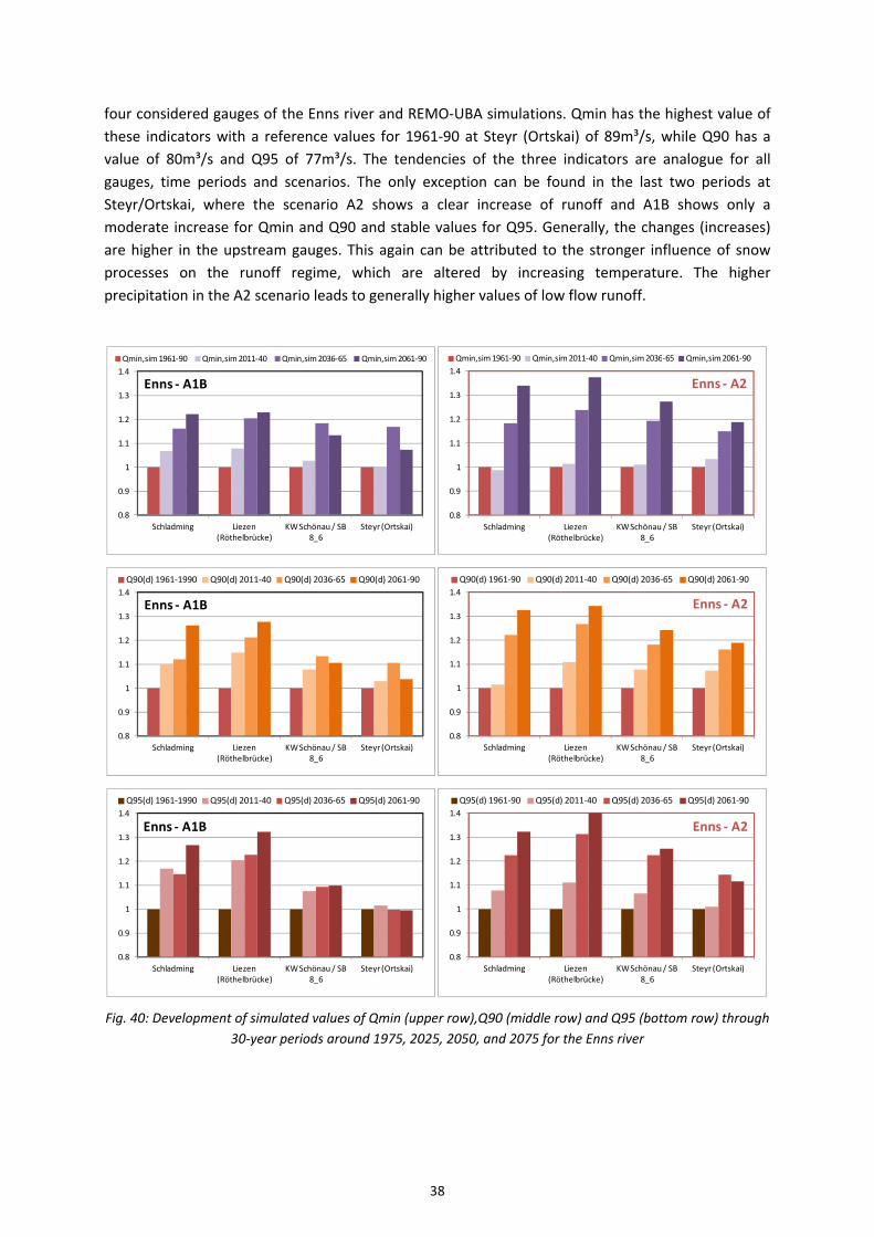
This implies rising low flow values under climate change assumptions for the 21st century. Fig. 40

shows the development of the three low flow runoff indicators Qmin (mean lowest monthly runoff in

a year), Q95 (runoff exceeded on 95% of the days) Q90 (runoff exceeded on 90% of the days) for the

0

10

20

30

40

50

1 2 3 4 5 6 7 8 9 10 11 12Runoff (m³/s)

Month

Ager

REMO‐UBA 2061‐2090

REMO‐UBA 1961‐1990

0

10

20

30

40

50

1 2 3 4 5 6 7 8 9 10 11 12

Runoff (m³/s)

Month

Ager

RegCM3 1961‐1990

RegCM3 2061‐2090

0

10

20

30

40

50

1 2 3 4 5 6 7 8 9 10 11 12

Runoff (m³/s)

Month

Ager

Aladin‐Arpege 1961‐1990


10

100

1000

0.00 0.20 0.40 0.60 0.80 1.00

Runoff [m³/s]


Enns A1B (Liezen)

d_Qsim 1961‐1990d_Qsim 2011‐40d_Qsim 2036‐65d_Qsim 2061‐90

10

100

1000

0.00 0.20 0.40 0.60 0.80 1.00

Runoff [m³/s]


Enns A2 (Liezen)

d_Qsim 1961‐90d_Qsim 2011‐40d_Qsim 2036‐65d_Qsim 2061‐90

38

four considered gauges of the Enns river and REMO‐UBA simulations. Qmin has the highest value of

these indicators with a reference values for 1961‐90 at Steyr (Ortskai) of 89m³/s, while Q90 has a

value of 80m³/s and Q95 of 77m³/s. The tendencies of the three indicators are analogue for all

gauges, time periods and scenarios. The only exception can be found in the last two periods at

Steyr/Ortskai, where the scenario A2 shows a clear increase of runoff and A1B shows only a

moderate increase for Qmin and Q90 and stable values for Q95. Generally, the changes (increases)

are higher in the upstream gauges. This again can be attributed to the stronger influence of snow

processes on the runoff regime, which are altered by increasing temperature. The higher

precipitation in the A2 scenario leads to generally higher values of low flow runoff.

Fig. 40: Development of simulated values of Qmin (upper row),Q90 (middle row) and Q95 (bottom row) through

30‐year periods around 1975, 2025, 2050, and 2075 for the Enns river

0.8

0.9

1

1.1

1.2

1.3

1.4



Steyr (Ortskai)

Enns ‐ A1B

Qmin,sim 1961‐90 Qmin,sim 2011‐40 Qmin,sim 2036‐65 Qmin,sim 2061‐90

0.8

0.9

1

1.1

1.2

1.3

1.4



Steyr (Ortskai)

Enns ‐ A2


0.8

0.9

1

1.1

1.2

1.3

1.4



Steyr (Ortskai)

Enns ‐ A1B

Q90(d) 1961‐1990 Q90(d) 2011‐40 Q90(d) 2036‐65 Q90(d) 2061‐90

0.8

0.9

1

1.1

1.2

1.3

1.4



Steyr (Ortskai)

Enns ‐ A2

Q90(d) 1961‐90 Q90(d) 2011‐40 Q90(d) 2036‐65 Q90(d) 2061‐90

0.8

0.9

1

1.1

1.2

1.3

1.4



Steyr (Ortskai)

Enns ‐ A1B

Q95(d) 1961‐1990 Q95(d) 2011‐40 Q95(d) 2036‐65 Q95(d) 2061‐90

0.8

0.9

1

1.1

1.2

1.3

1.4



Steyr (Ortskai)

Enns ‐ A2

Q95(d) 1961‐90 Q95(d) 2011‐40 Q95(d) 2036‐65 Q95(d) 2061‐90

39

Due to the comparable tendencies in all three indicators, only Qmin is shown for the comparison of

A1B and A2 scenarios of REMO‐UBA for the rivers Mur (Fig. 42) and Drau (Fig. 41). For both rivers we

again see increasing low flow runoff for all gauges and both scenarios, in almost all time periods, but

consistently for the second half of the 21st century. In the A2 scenario the increase is slightly higher

than in the A1B scenario, again. For the Mur, like for the Enns, the changes are more pronounced in

the more alpine upper reaches. For the Drau, there are almost no differences between the

projections for the different gauges.

Fig. 41: Development of simulated values of Qmin through 30‐year periods around 1975, 2025, 2050, and 2075

for the Mur river

Fig. 42: Development of simulated values of Qmin through 30‐year periods around 1975, 2025, 2050, and 2075

for the Drau river

The comparison between results for Qmin with different climate models for 2061‐2090 (Fig. 43)

reveals larger discrepancies. In this analysis, the Ager basin is included again.

For the Enns (Fig. 43, top left), RegCM3 shows even larger increases in low flow runoff than

REMO‐UBA. With Aladin‐Arpege, low flow runoff increase only marginally, and for the most

downstream gauge even a slight decrease is expected. In scenarios with all three models more

pronounced changes are simulated for the more headwater reaches.

Lower low flow runoff with Aladin‐Arpege than with the other two models is also simulated in the

other analysed basins. This can be connected with the less pronounced increase in winter runoff in

the basins with alpine influence with this model (as shown in Fig. 35, Fig. 36, Fig. 37), as low flow

0.8

0.9

1

1.1

1.2

1.3

1.4



Judenburg


unter Mürz


Mur ‐ A1B


0.8

0.9

1

1.1

1.2

1.3

1.4



Judenburg


unter Mürz


Mur ‐ A2


0.8

0.9

1

1.1

1.2

1.3

1.4


Villach Lavamünd

Drau ‐ A1B


0.8

0.9

1

1.1

1.2

1.3

1.4


Villach Lavamünd

Drau ‐ A2


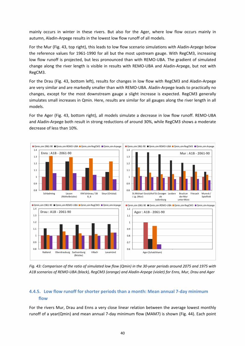
40

mainly occurs in winter in these rivers. But also for the Ager, where low flow occurs mainly in

autumn, Aladin‐Arpege results in the lowest low flow runoff of all models.

For the Mur (Fig. 43, top right), this leads to low flow scenario simulations with Aladin‐Arpege below

the reference values for 1961‐1990 for all but the most upstream gauge. With RegCM3, increasing

low flow runoff is projected, but less pronounced than with REMO‐UBA. The gradient of simulated

change along the river length is visible in results with REMO‐UBA and Aladin‐Arpege, but not with

RegCM3.

For the Drau (Fig. 43, bottom left), results for changes in low flow with RegCM3 and Aladin‐Arpege

are very similar and are markedly smaller than with REMO‐UBA. Aladin‐Arpege leads to practically no

changes, except for the most downstream gauge a slight increase is expected. RegCM3 generally

simulates small increases in Qmin. Here, results are similar for all gauges along the river length in all

models.

For the Ager (Fig. 43, bottom right), all models simulate a decrease in low flow runoff. REMO‐UBA

and Aladin‐Arpege both result in strong reductions of around 30%, while RegCM3 shows a moderate

decrease of less than 10%.

Fig. 43: Comparison of the ratio of simulated low flow (Qmin) in the 30‐year periods around 2075 and 1975 with

A1B scenarios of REMO‐UBA (black), RegCM3 (orange) and Aladin‐Arpege (violet) for Enns, Mur, Drau and Ager

4.4.5. Low flow runoff for shorter periods than a month: Mean annual 7‐day minimum

flow

For the rivers Mur, Drau and Enns a very close linear relation between the average lowest monthly

runoff of a year(Qmin) and mean annual 7‐day minimum flow (MAM7) is shown (Fig. 44). Each point

0.8

0.9

1

1.1

1.2

1.3

1.4



Steyr (Ortskai)

Enns : A1B ‐ 2061‐90

Qmin,sim 1961‐90 Qmin,sim REMO‐UBA Qmin,sim RegCM3 Qmin,sim Arpege

0.8

0.9

1

1.1

1.2

1.3

1.4



Judenburg


unter Mürz


Mur : A1B ‐ 2061‐90


0.8

0.9

1

1.1

1.2

1.3

1.4


Villach Lavamünd

Drau : A1B ‐ 2061‐90


0.6

0.7

0.8

0.9

1

1.1

1.2

Ager (Schalchham)

Ager : A1B ‐ 2061‐90


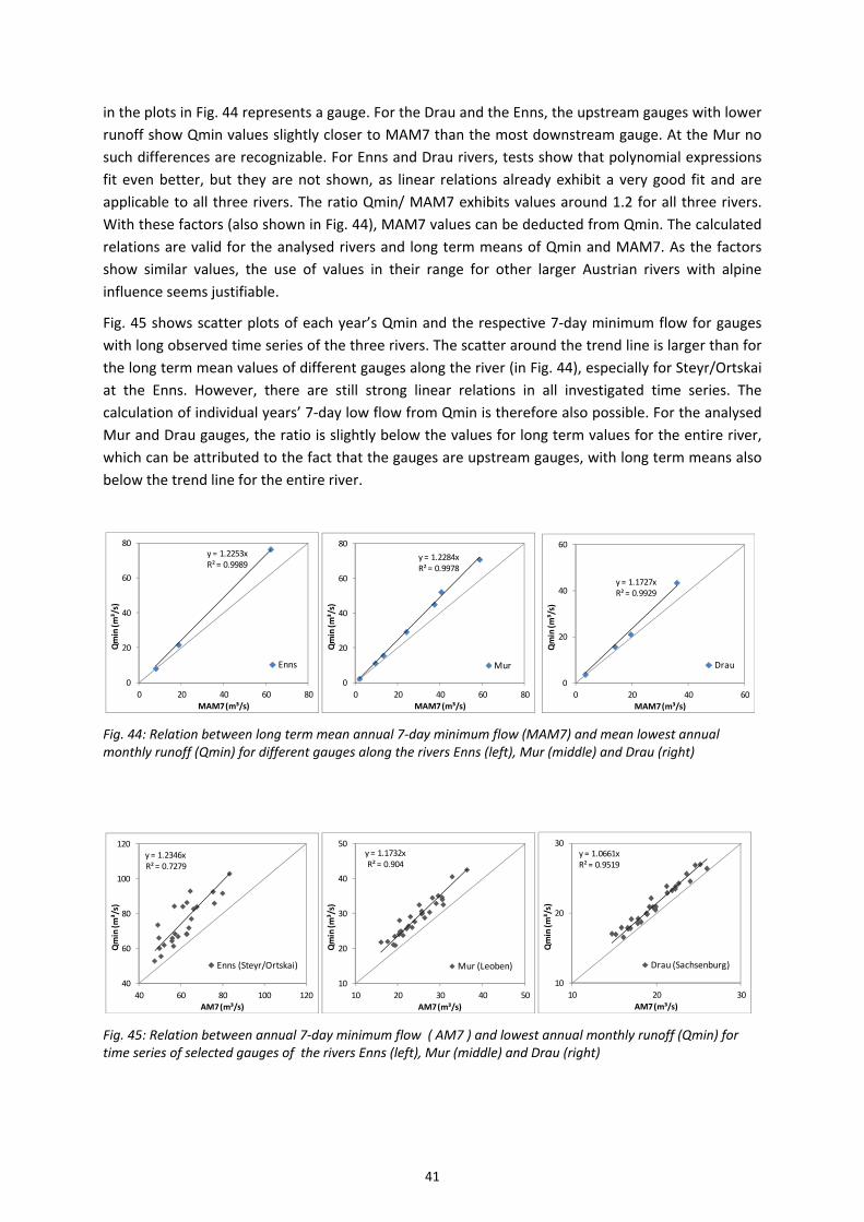
41

in the plots in Fig. 44 represents a gauge. For the Drau and the Enns, the upstream gauges with lower

runoff show Qmin values slightly closer to MAM7 than the most downstream gauge. At the Mur no

such differences are recognizable. For Enns and Drau rivers, tests show that polynomial expressions

fit even better, but they are not shown, as linear relations already exhibit a very good fit and are

applicable to all three rivers. The ratio Qmin/ MAM7 exhibits values around 1.2 for all three rivers.

With these factors (also shown in Fig. 44), MAM7 values can be deducted from Qmin. The calculated

relations are valid for the analysed rivers and long term means of Qmin and MAM7. As the factors

show similar values, the use of values in their range for other larger Austrian rivers with alpine

influence seems justifiable.

Fig. 45 shows scatter plots of each year’s Qmin and the respective 7‐day minimum flow for gauges

with long observed time series of the three rivers. The scatter around the trend line is larger than for

the long term mean values of different gauges along the river (in Fig. 44), especially for Steyr/Ortskai

at the Enns. However, there are still strong linear relations in all investigated time series. The

calculation of individual years’ 7‐day low flow from Qmin is therefore also possible. For the analysed

Mur and Drau gauges, the ratio is slightly below the values for long term values for the entire river,

which can be attributed to the fact that the gauges are upstream gauges, with long term means also

below the trend line for the entire river.

Fig. 44: Relation between long term mean annual 7‐day minimum flow (MAM7) and mean lowest annual monthly runoff (Qmin) for different gauges along the rivers Enns (left), Mur (middle) and Drau (right)

Fig. 45: Relation between annual 7‐day minimum flow ( AM7 ) and lowest annual monthly runoff (Qmin) for time series of selected gauges of the rivers Enns (left), Mur (middle) and Drau (right)

y = 1.2253xR² = 0.9989

0

20

40

60

80

0 20 40 60 80

Qmin (m

³/s)

MAM7 (m³/s)

Enns

y = 1.2284xR² = 0.9978

0

20

40

60

80

0 20 40 60 80

Qmin (m

³/s)

MAM7 (m³/s)

Mur

y = 1.1727xR² = 0.9929

0

20

40

60

0 20 40 60

Qmin (m

³/s)

MAM7 (m³/s)

Drau

y = 1.2346xR² = 0.7279

40

60

80

100

120

40 60 80 100 120

Qmin (m

³/s)

AM7 (m³/s)

Enns (Steyr/Ortskai)

y = 1.1732xR² = 0.904

10

20

30

40

50

10 20 30 40 50

Qmin (m

³/s)

AM7 (m³/s)

Mur (Leoben)

y = 1.0661xR² = 0.9519

10

20

30

10 20 30

Qmin (m

³/s)

AM7 (m³/s)

Drau (Sachsenburg)

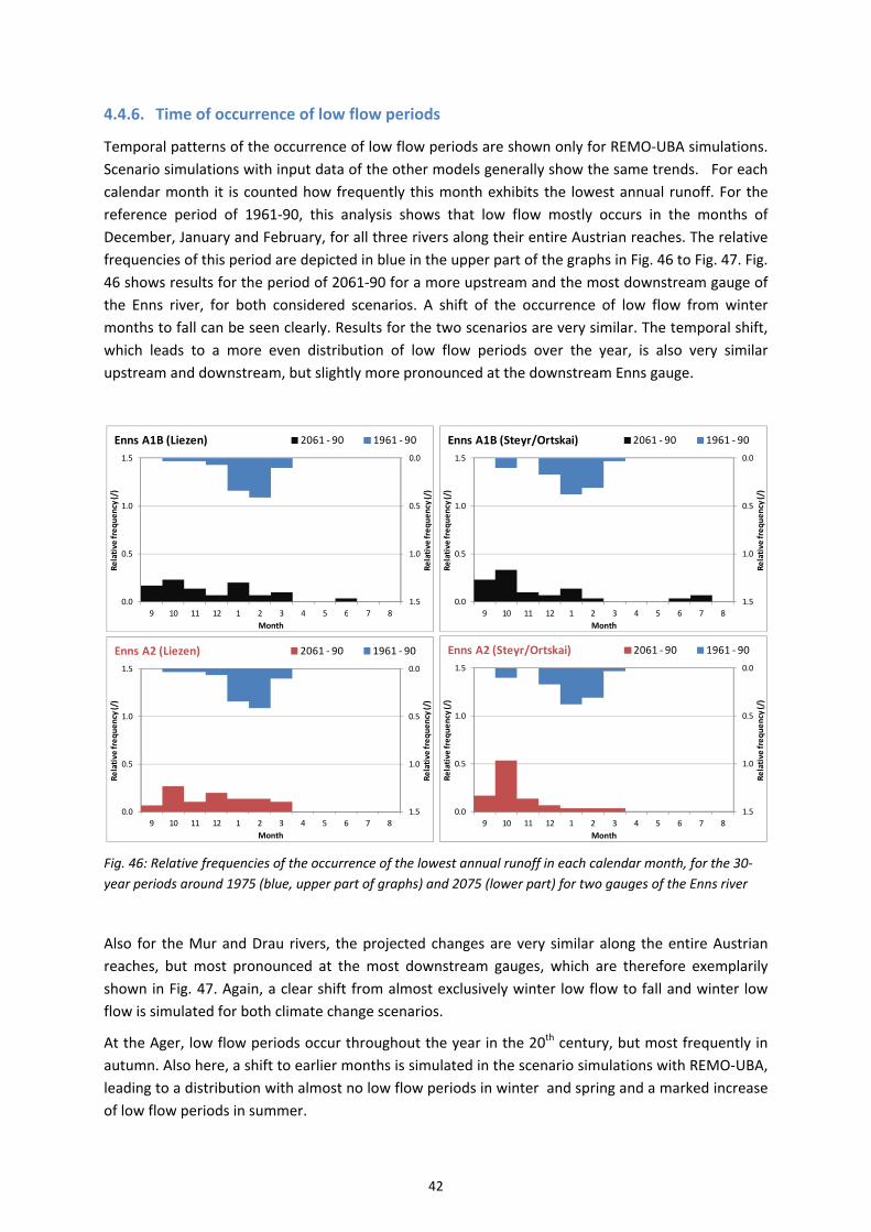
42

4.4.6. Time of occurrence of low flow periods

Temporal patterns of the occurrence of low flow periods are shown only for REMO‐UBA simulations.

Scenario simulations with input data of the other models generally show the same trends. For each

calendar month it is counted how frequently this month exhibits the lowest annual runoff. For the

reference period of 1961‐90, this analysis shows that low flow mostly occurs in the months of

December, January and February, for all three rivers along their entire Austrian reaches. The relative

frequencies of this period are depicted in blue in the upper part of the graphs in Fig. 46 to Fig. 47. Fig.

46 shows results for the period of 2061‐90 for a more upstream and the most downstream gauge of

the Enns river, for both considered scenarios. A shift of the occurrence of low flow from winter

months to fall can be seen clearly. Results for the two scenarios are very similar. The temporal shift,

which leads to a more even distribution of low flow periods over the year, is also very similar

upstream and downstream, but slightly more pronounced at the downstream Enns gauge.

Fig. 46: Relative frequencies of the occurrence of the lowest annual runoff in each calendar month, for the 30‐

year periods around 1975 (blue, upper part of graphs) and 2075 (lower part) for two gauges of the Enns river

Also for the Mur and Drau rivers, the projected changes are very similar along the entire Austrian

reaches, but most pronounced at the most downstream gauges, which are therefore exemplarily

shown in Fig. 47. Again, a clear shift from almost exclusively winter low flow to fall and winter low

flow is simulated for both climate change scenarios.

At the Ager, low flow periods occur throughout the year in the 20th century, but most frequently in

autumn. Also here, a shift to earlier months is simulated in the scenario simulations with REMO‐UBA,

leading to a distribution with almost no low flow periods in winter and spring and a marked increase

of low flow periods in summer.

0.0

0.5

1.0

1.50.0

0.5

1.0

1.5

9 10 11 12 1 2 3 4 5 6 7 8

Relative

frequency (/)

Relative

frequency (/)

Month

Enns A1B (Liezen) 2061 ‐ 90 1961 ‐ 90

0.0

0.5

1.0

1.50.0

0.5

1.0

1.5

9 10 11 12 1 2 3 4 5 6 7 8

Relative

frequency (/)

Relative

frequency (/)

Month

Enns A1B (Steyr/Ortskai) 2061 ‐ 90 1961 ‐ 90

0.0

0.5

1.0

1.50.0

0.5

1.0

1.5

9 10 11 12 1 2 3 4 5 6 7 8

Relative

frequency (/)

Relative

frequency (/)

Month

Enns A2 (Liezen) 2061 ‐ 90 1961 ‐ 90

0.0

0.5

1.0

1.50.0

0.5

1.0

1.5

9 10 11 12 1 2 3 4 5 6 7 8

Relative

frequency (/)

Relative

frequency (/)

Month

Enns A2 (Steyr/Ortskai) 2061 ‐ 90 1961 ‐ 90

43


year periods around 1975 and 2075 for the most downstream gauges of the Mur and Drau rivers


year periods around 1975 and 2075 for the Ager rivers

4.4.7. Low flow duration under climate change conditions

The run lengths of low flow periods, defined as months with discharge below Q90 of the respective

30‐year period, is assessed for the Enns and Drau rivers. The skewness measures g of the run length

distributions (Fig. 49) exhibit increases in the scenario simulations of both basins with REMO‐UBA,

because higher values of run length of 5 to 7 months occur (the highest value in the reference period

is 4 months). These high values occur only one to two times in 30 years. Within the 21st century,

there is a decreasing tendency of g for both REMO‐UBA scenarios for the Enns. For the Drau, the

REMO‐UBA A1B and the RegCM3 scenarios also exhibit this decreasing trend within the 21st century,

0.0

0.5

1.0

1.50.0

0.5

1.0

1.5

9 10 11 12 1 2 3 4 5 6 7 8

Relative

frequency (/)

Relative

frequency (/)

Month

Mur A1B (Mureck/Spielfeld) 2061 ‐ 90 1961 ‐ 90

0.0

0.5

1.0

1.50.0

0.5

1.0

1.5

9 10 11 12 1 2 3 4 5 6 7 8

Relative

frequency (/)

Relative

frequency (/)

Month

Mur A2 (Mureck/Spielfeld) 2061 ‐ 90 1961 ‐ 90

0.0

0.5

1.0

1.50.0

0.5

1.0

1.5

9 10 11 12 1 2 3 4 5 6 7 8

Relative

frequency (/)

Relative

frequency (/)

Month

Drau A1B (Lavamünd) 2061‐90 1961 ‐ 90

0.0

0.5

1.0

1.50.0

0.5

1.0

1.5

9 10 11 12 1 2 3 4 5 6 7 8

Relative

frequency (/)

Relative

frequency (/)

Month

Drau A2 (Lavamünd) 2061 ‐ 90 1961 ‐ 90

0.0

0.5

1.0

1.50.0

0.5

1.0

1.5

9 10 11 12 1 2 3 4 5 6 7 8

Relative

frequency (/)

Relative

frequency (/)

Month

Ager A1B 2061 ‐ 90 1961‐1990

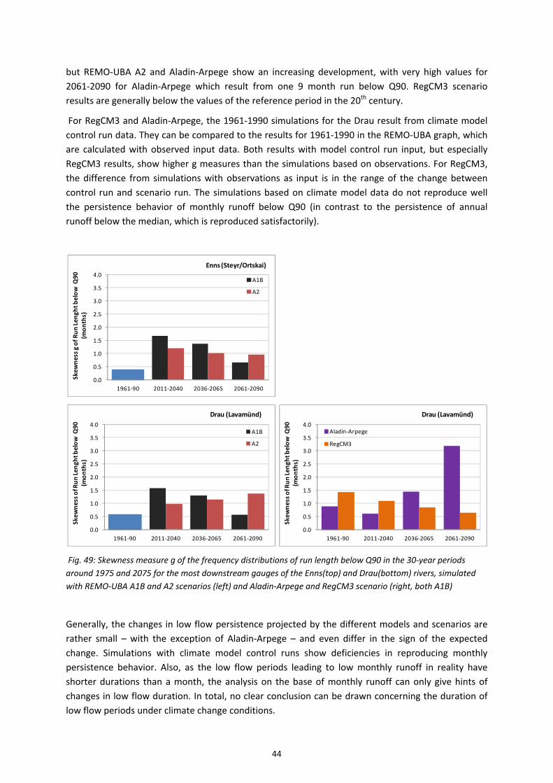
44

but REMO‐UBA A2 and Aladin‐Arpege show an increasing development, with very high values for

2061‐2090 for Aladin‐Arpege which result from one 9 month run below Q90. RegCM3 scenario

results are generally below the values of the reference period in the 20th century.

For RegCM3 and Aladin‐Arpege, the 1961‐1990 simulations for the Drau result from climate model

control run data. They can be compared to the results for 1961‐1990 in the REMO‐UBA graph, which

are calculated with observed input data. Both results with model control run input, but especially

RegCM3 results, show higher g measures than the simulations based on observations. For RegCM3,

the difference from simulations with observations as input is in the range of the change between

control run and scenario run. The simulations based on climate model data do not reproduce well

the persistence behavior of monthly runoff below Q90 (in contrast to the persistence of annual

runoff below the median, which is reproduced satisfactorily).

Fig. 49: Skewness measure g of the frequency distributions of run length below Q90 in the 30‐year periods

around 1975 and 2075 for the most downstream gauges of the Enns(top) and Drau(bottom) rivers, simulated

with REMO‐UBA A1B and A2 scenarios (left) and Aladin‐Arpege and RegCM3 scenario (right, both A1B)

Generally, the changes in low flow persistence projected by the different models and scenarios are

rather small – with the exception of Aladin‐Arpege – and even differ in the sign of the expected

change. Simulations with climate model control runs show deficiencies in reproducing monthly

persistence behavior. Also, as the low flow periods leading to low monthly runoff in reality have

shorter durations than a month, the analysis on the base of monthly runoff can only give hints of

changes in low flow duration. In total, no clear conclusion can be drawn concerning the duration of

low flow periods under climate change conditions.

0.0

0.5

1.0

1.5

2.0

2.5

3.0

3.5

4.0

1961‐90 2011‐2040 2036‐2065 2061‐2090

Skewness g of Run Len

ght below Q

90

(months)


A1B

A2

0.0

0.5

1.0

1.5

2.0

2.5

3.0

3.5

4.0

1961‐90 2011‐2040 2036‐2065 2061‐2090

Skewness of Run Len

ght below Q

90

(months)

Drau (Lavamünd)

A1B

A2

0.0

0.5

1.0

1.5

2.0

2.5

3.0

3.5

4.0

1961‐90 2011‐2040 2036‐2065 2061‐2090

Skewness of Run Len

ght below Q

90

(months)

Drau (Lavamünd)

Aladin‐Arpege

RegCM3

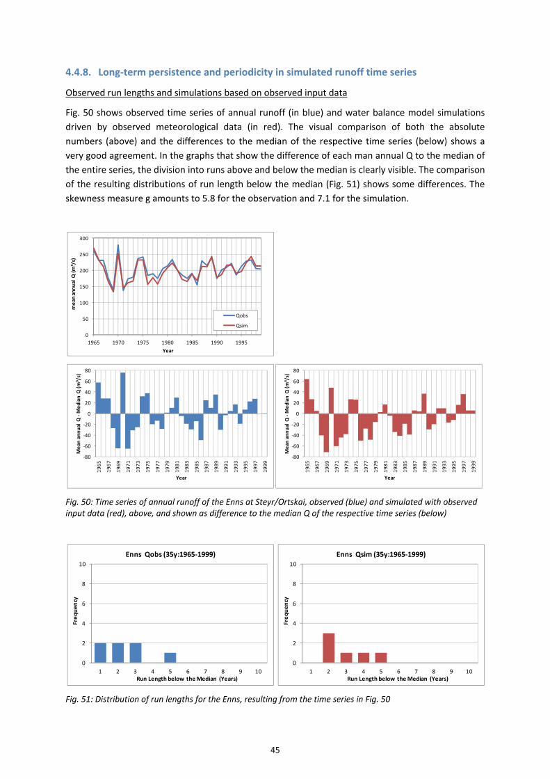
45

4.4.8. Long‐term persistence and periodicity in simulated runoff time series

Observed run lengths and simulations based on observed input data

Fig. 50 shows observed time series of annual runoff (in blue) and water balance model simulations

driven by observed meteorological data (in red). The visual comparison of both the absolute

numbers (above) and the differences to the median of the respective time series (below) shows a

very good agreement. In the graphs that show the difference of each man annual Q to the median of

the entire series, the division into runs above and below the median is clearly visible. The comparison

of the resulting distributions of run length below the median (Fig. 51) shows some differences. The

skewness measure g amounts to 5.8 for the observation and 7.1 for the simulation.

Fig. 50: Time series of annual runoff of the Enns at Steyr/Ortskai, observed (blue) and simulated with observed input data (red), above, and shown as difference to the median Q of the respective time series (below)

Fig. 51: Distribution of run lengths for the Enns, resulting from the time series in Fig. 50

0

50

100

150

200

250

300

1965 1970 1975 1980 1985 1990 1995

mean

annual Q

(m³/s)

Year

Qobs

Qsim

‐80

‐60

‐40

‐20

0

20

40

60

80

1965

1967

1969

1971

1973

1975

1977

1979

1981

1983

1985

1987

1989

1991

1993

1995

1997

1999

Mean

annual Q

‐Median Q

(m³/s)

Year

‐80

‐60

‐40

‐20

0

20

40

60

80

1965

1967

1969

1971

1973

1975

1977

1979

1981

1983

1985

1987

1989

1991

1993

1995

1997

1999

Mean

annual Q

‐Median Q

(m³/s)

Year

0

2

4

6

8

10

1 2 3 4 5 6 7 8 9 10

Frequency


Enns Qobs (35y:1965‐1999)

0

2

4

6

8

10

1 2 3 4 5 6 7 8 9 10

Frequency


Enns Qsim (35y:1965‐1999)

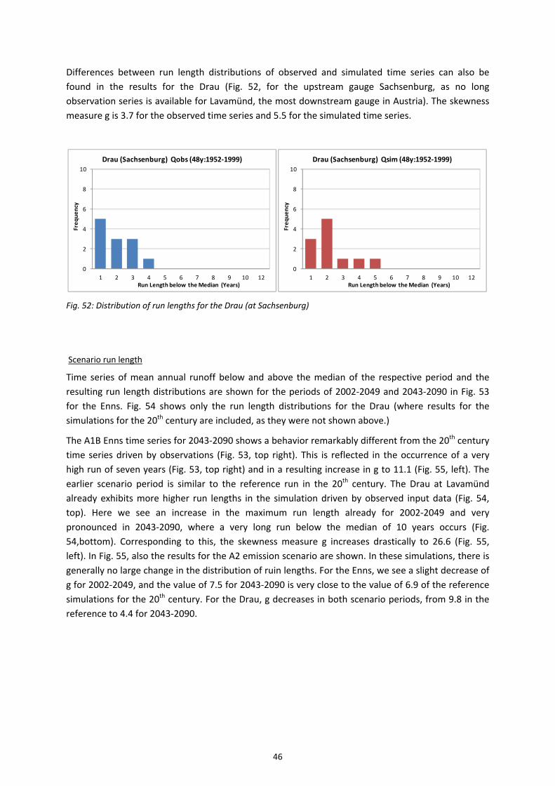
46

Differences between run length distributions of observed and simulated time series can also be

found in the results for the Drau (Fig. 52, for the upstream gauge Sachsenburg, as no long

observation series is available for Lavamünd, the most downstream gauge in Austria). The skewness

measure g is 3.7 for the observed time series and 5.5 for the simulated time series.

Fig. 52: Distribution of run lengths for the Drau (at Sachsenburg)

Scenario run length

Time series of mean annual runoff below and above the median of the respective period and the

resulting run length distributions are shown for the periods of 2002‐2049 and 2043‐2090 in Fig. 53

for the Enns. Fig. 54 shows only the run length distributions for the Drau (where results for the

simulations for the 20th century are included, as they were not shown above.)

The A1B Enns time series for 2043‐2090 shows a behavior remarkably different from the 20th century

time series driven by observations (Fig. 53, top right). This is reflected in the occurrence of a very

high run of seven years (Fig. 53, top right) and in a resulting increase in g to 11.1 (Fig. 55, left). The

earlier scenario period is similar to the reference run in the 20th century. The Drau at Lavamünd

already exhibits more higher run lengths in the simulation driven by observed input data (Fig. 54,

top). Here we see an increase in the maximum run length already for 2002‐2049 and very

pronounced in 2043‐2090, where a very long run below the median of 10 years occurs (Fig.

54,bottom). Corresponding to this, the skewness measure g increases drastically to 26.6 (Fig. 55,

left). In Fig. 55, also the results for the A2 emission scenario are shown. In these simulations, there is

generally no large change in the distribution of ruin lengths. For the Enns, we see a slight decrease of

g for 2002‐2049, and the value of 7.5 for 2043‐2090 is very close to the value of 6.9 of the reference

simulations for the 20th century. For the Drau, g decreases in both scenario periods, from 9.8 in the

reference to 4.4 for 2043‐2090.

0

2

4

6

8

10

1 2 3 4 5 6 7 8 9 10 12

Frequency


Drau (Sachsenburg) Qobs (48y:1952‐1999)

0

2

4

6

8

10

1 2 3 4 5 6 7 8 9 10 12

Frequency


Drau (Sachsenburg) Qsim (48y:1952‐1999)

47

Fig. 53: Difference between mean annual runoff and the median for the respective period for 2002‐2043 (left) and 2049‐2090 (right), above; resulting distributions of run lengths, below; REMO‐UBA A1B for the Enns at Styr/Ortskai

Fig. 54: Distribution of run lengths in simulated runoff for the periods of 1952‐1999, (top left, blue) and 2002‐2049 (bottom left) and 2043‐2090 (bottom right); REMO‐UBA A1B for the Drau at Lavamünd

‐80

‐60

‐40

‐20

0

20

40

60

80

2002

2004

2006

2008

2010

2012

2014

2016

2018

2020

2022

2024

2026

2028

2030

2032

2034

2036

2038

2040

2042

2044

2046

2048

Mean

annual Q

‐Median Q

(m³/s)

Year

‐80

‐60

‐40

‐20

0

20

40

60

80

2043

2045

2047

2049

2051

2053

2055

2057

2059

2061

2063

2065

2067

2069

2071

2073

2075

2077

2079

2081

2083

2085

2087

2089

Mean

annual Q

‐Median Q

(m³/s)

Year

0

1

2

3

4

5

6

7

8

9

10

1 2 3 4 5 6 7 8 9 10

Frequency


Enns Qsim (48y: 2002‐49)

0

1

2

3

4

5

6

7

8

9

10

1 2 3 4 5 6 7 8 9 10

Frequency


Enns Qsim (48y: 2043‐90)

0

1

2

3

4

5

6

7

8

9

10

1 2 3 4 5 6 7 8 9 10

Frequency


Drau (Lavamünd) Qsim (48y: 1952‐99)

0

1

2

3

4

5

6

7

8

9

10

1 2 3 4 5 6 7 8 9 10

Frequency



0

1

2

3

4

5

6

7

8

9

10

1 2 3 4 5 6 7 8 9 10

Frequency



48

Fig. 55: Skewness measure g for the distributions of run lengths in simulated runoff for the periods of 1952‐1999 (blue) and 2002‐2049 and 2043‐2090 (REMO‐UBA, black: A1B, red: A2), for the Enns (left) and the Drau (right)

In the analysis of water balance simulations driven by Aladin‐Arpege and RegCM3 climate data,

results with control run data can be included. Fig. 56 shows the two control run simulations for the

Drau (depicted as the difference between mean annual Q and the median of the entire period). It is

clearly visible, that the sequences are different in the two simulations, resulting from different and

random “weather” in each model (only the long term means are expected to be the same or very

similar). The amplitudes are markedly higher in the simulations driven by Aladin‐Arpege data (Fig. 56,

left) than in the RegCM3 results (Fig. 56, right). The resulting values of g of the run length

distributions (Fig. 57), however, are close to each other (11.1 for Aladin‐Arpege and 9.8 for RegCM3)

and also very close to the simulations driven by observed climate data (9.8). This means that the

water balance simulations driven by climate model control run data generally show a long‐term

persistence behavior in accordance with observations and simulations with observed climate data.

Fig. 56: Mean annual runoff time series (mean annual Q ‐ median Q of the entire period) for the simulations with control run climate model data for Aladin‐Arpege (left) and RegCM3 (right).

The distributions of run lengths in the scenario simulations of the two models, as described by the

value of g (Fig. 57), are also rather close to each other. For the period of 2002‐2049, they both show

a decline of g, which is in contrast to the slight increase in the REMO‐UBA A1B simulations. For the

more distant period of 2043‐2090, with a stronger climate change signal, they both show an increase

0

5

10

15

20

25

30

1952‐1999 2002‐2049 2043‐2090

Skewness of Run Lenght below M

edian


A1B

A2

0

5

10

15

20

25

30

1952‐1999 2002‐2049 2043‐2090


edian

Drau (Lavamünd)

A1B

A2

‐100

‐80

‐60

‐40

‐20

0

20

40

60

80

100

1952

1954

1956

1958

1960

1962

1964

1966

1968

1970

1972

1974

1976

1978

1980

1982

1984

1986

1988

1990

1992

1994

1996

1998

Mean

annual Q

‐Median Q

(m³/s)

Year

‐100

‐80

‐60

‐40

‐20

0

20

40

60

80

100

1952

1954

1956

1958

1960

1962

1964

1966

1968

1970

1972

1974

1976

1978

1980

1982

1984

1986

1988

1990

1992

1994

1996

1998

Mean

annual Q

‐Median Q

(m³/s)

Year

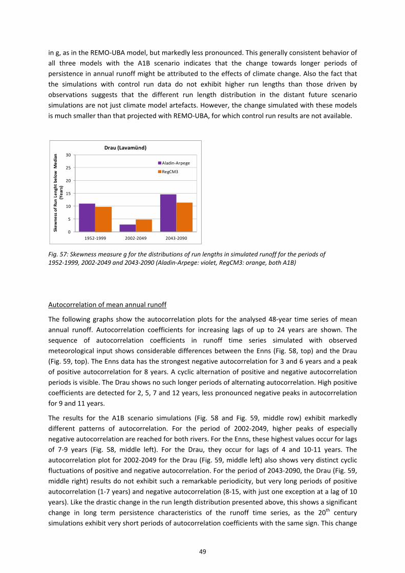
49

in g, as in the REMO‐UBA model, but markedly less pronounced. This generally consistent behavior of

all three models with the A1B scenario indicates that the change towards longer periods of

persistence in annual runoff might be attributed to the effects of climate change. Also the fact that

the simulations with control run data do not exhibit higher run lengths than those driven by

observations suggests that the different run length distribution in the distant future scenario

simulations are not just climate model artefacts. However, the change simulated with these models

is much smaller than that projected with REMO‐UBA, for which control run results are not available.

Fig. 57: Skewness measure g for the distributions of run lengths in simulated runoff for the periods of 1952‐1999, 2002‐2049 and 2043‐2090 (Aladin‐Arpege: violet, RegCM3: orange, both A1B)

Autocorrelation of mean annual runoff

The following graphs show the autocorrelation plots for the analysed 48‐year time series of mean

annual runoff. Autocorrelation coefficients for increasing lags of up to 24 years are shown. The

sequence of autocorrelation coefficients in runoff time series simulated with observed

meteorological input shows considerable differences between the Enns (Fig. 58, top) and the Drau

(Fig. 59, top). The Enns data has the strongest negative autocorrelation for 3 and 6 years and a peak

of positive autocorrelation for 8 years. A cyclic alternation of positive and negative autocorrelation

periods is visible. The Drau shows no such longer periods of alternating autocorrelation. High positive

coefficients are detected for 2, 5, 7 and 12 years, less pronounced negative peaks in autocorrelation

for 9 and 11 years.

The results for the A1B scenario simulations (Fig. 58 and Fig. 59, middle row) exhibit markedly

different patterns of autocorrelation. For the period of 2002‐2049, higher peaks of especially

negative autocorrelation are reached for both rivers. For the Enns, these highest values occur for lags

of 7‐9 years (Fig. 58, middle left). For the Drau, they occur for lags of 4 and 10‐11 years. The

autocorrelation plot for 2002‐2049 for the Drau (Fig. 59, middle left) also shows very distinct cyclic

fluctuations of positive and negative autocorrelation. For the period of 2043‐2090, the Drau (Fig. 59,

middle right) results do not exhibit such a remarkable periodicity, but very long periods of positive

autocorrelation (1‐7 years) and negative autocorrelation (8‐15, with just one exception at a lag of 10

years). Like the drastic change in the run length distribution presented above, this shows a significant

change in long term persistence characteristics of the runoff time series, as the 20th century

simulations exhibit very short periods of autocorrelation coefficients with the same sign. This change

0

5

10

15

20

25

30

1952‐1999 2002‐2049 2043‐2090


edian

(Years)

Drau (Lavamünd)

Aladin‐Arpege

RegCM3

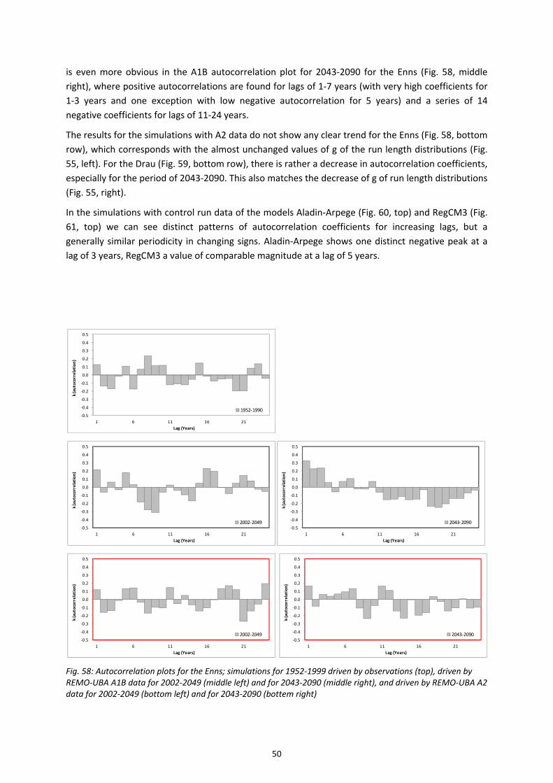
50

is even more obvious in the A1B autocorrelation plot for 2043‐2090 for the Enns (Fig. 58, middle

right), where positive autocorrelations are found for lags of 1‐7 years (with very high coefficients for

1‐3 years and one exception with low negative autocorrelation for 5 years) and a series of 14

negative coefficients for lags of 11‐24 years.

The results for the simulations with A2 data do not show any clear trend for the Enns (Fig. 58, bottom

row), which corresponds with the almost unchanged values of g of the run length distributions (Fig.

55, left). For the Drau (Fig. 59, bottom row), there is rather a decrease in autocorrelation coefficients,

especially for the period of 2043‐2090. This also matches the decrease of g of run length distributions

(Fig. 55, right).

In the simulations with control run data of the models Aladin‐Arpege (Fig. 60, top) and RegCM3 (Fig.

61, top) we can see distinct patterns of autocorrelation coefficients for increasing lags, but a

generally similar periodicity in changing signs. Aladin‐Arpege shows one distinct negative peak at a

lag of 3 years, RegCM3 a value of comparable magnitude at a lag of 5 years.

Fig. 58: Autocorrelation plots for the Enns; simulations for 1952‐1999 driven by observations (top), driven by REMO‐UBA A1B data for 2002‐2049 (middle left) and for 2043‐2090 (middle right), and driven by REMO‐UBA A2 data for 2002‐2049 (bottom left) and for 2043‐2090 (bottem right)

‐0.5

‐0.4

‐0.3

‐0.2

‐0.1

0.0

0.1

0.2

0.3

0.4

0.5

1 6 11 16 21

k (autocorrelation)

Lag (Years)

1952‐1990

‐0.5

‐0.4

‐0.3

‐0.2

‐0.1

0.0

0.1

0.2

0.3

0.4

0.5

1 6 11 16 21

k (autocorrelation)

Lag (Years)

2002‐2049‐0.5

‐0.4

‐0.3

‐0.2

‐0.1

0.0

0.1

0.2

0.3

0.4

0.5

1 6 11 16 21

k (autocorrelation)

Lag (Years)

2043‐2090

‐0.5

‐0.4

‐0.3

‐0.2

‐0.1

0.0

0.1

0.2

0.3

0.4

0.5

1 6 11 16 21

k (autocorrelation)

Lag (Years)

2002‐2049‐0.5

‐0.4

‐0.3

‐0.2

‐0.1

0.0

0.1

0.2

0.3

0.4

0.5

1 6 11 16 21

k (autocorrelation)

Lag (Years)

2043‐2090

51

Fig. 59: Autocorrelation plots for the Drau; simulations for 1952‐1999 driven by observations (top), driven by REMO‐UBA A1B data for 2002‐2049 (middle left) and for 2043‐2090 (middle right), and driven by REMO‐UBA A2 data for 2002‐2049 (bottom left) and for 2043‐2090 (bottem right)

Fig. 60: Autocorrelation plots for the Drau with Aladin‐Arpege; simulations for 1952‐1999 (top), for 2002‐2049 (bottom left) and for 2043‐2090 (bottem right)

‐0.5

‐0.4

‐0.3

‐0.2

‐0.1

0.0

0.1

0.2

0.3

0.4

0.5

1 6 11 16 21

k (autocorrelation)

Lag (Years)

1952‐1990

‐0.5

‐0.4

‐0.3

‐0.2

‐0.1

0.0

0.1

0.2

0.3

0.4

0.5

1 6 11 16 21

k (autocorrelation)

Lag (Years)

2002‐2049‐0.5

‐0.4

‐0.3

‐0.2

‐0.1

0.0

0.1

0.2

0.3

0.4

0.5

1 6 11 16 21

k (autocorrelation)

Lag (Years)

2043‐2090

‐0.5

‐0.4

‐0.3

‐0.2

‐0.1

0.0

0.1

0.2

0.3

0.4

0.5

1 6 11 16 21

k (autocorrelation)

Lag (Years)

2002‐2049‐0.5

‐0.4

‐0.3

‐0.2

‐0.1

0.0

0.1

0.2

0.3

0.4

0.5

1 6 11 16 21

k (autocorrelation)

Lag (Years)

2043‐2090

‐0.5

‐0.4

‐0.3

‐0.2

‐0.1

0.0

0.1

0.2

0.3

0.4

0.5

1 6 11 16 21

k (autocorrelation)

Lag (Years)

1952‐1990

‐0.5

‐0.4

‐0.3

‐0.2

‐0.1

0.0

0.1

0.2

0.3

0.4

0.5

1 6 11 16 21

k (autocorrelation)

Lag (Years)

2002‐2049‐0.5

‐0.4

‐0.3

‐0.2

‐0.1

0.0

0.1

0.2

0.3

0.4

0.5

1 6 11 16 21

k (autocorrelation)

Lag (Years)

2043‐2090

52

Fig. 61: Autocorrelation plots for the Drau with RegCM3; simulations for 1952‐1999 (top), for 2002‐2049 (bottom left) and for 2043‐2090 (bottem right)

The simulations for the period of 2002‐2049 (Fig. 60 and Fig. 61, bottom left) show autocorrelation

coefficients lower than in the control run simulations for both models, which corresponds with

decreasing g of the run length distributions (Fig. 57). The increasing values of the coefficients and the

more pronounced periodicity in the period of 2043‐2090 is better visible in the Aladin‐Arpege

simulations (Fig. 60, bottom right) than in those of RegCM3 (Fig. 61, bottom right). This also

corresponds with the more pronounced increase in the g value of run length distributions for

Aladin‐Arpege (Fig. 57).

4.5. Alpine reservoirs

For all three considered reservoir systems the development of runoff and precipitation, liquid and

solid precipitation portions, snow accumulation and snow melt and the runoff contributions of snow

melt and glacier melt are described. These results are based mainly on REMO‐UBA A1B climate

change scenarios. For the catchment areas of the Gepatsch reservoir, a more detailed analysis of

glacier development is conducted, comparing results with different ice melt DDFs and with different

emission scenarios and different climate models. Therefore, the results for Gepatsch are displayed

first and described in more detail. The main results for Sellrain‐Silz and Kaprun‐Uttendorf are then

presented briefly.

4.5.1. Gepatsch

Fig. 62 shows the expected seasonal changes in precipitation (liquid and solid) and runoff. While for

precipitation only minor changes are projected – slight increase in winter and decreases in summer –

the runoff pattern changes drastically. In 2011‐40, there is almost no change yet, the slightly higher

runoff in summer can mainly be attributed to glacier melt. In 2036‐65, the trend to a decrease of the

summer peak and an increase of spring runoff is already visible. In 2061‐90, summer runoff is much

lower than in the reference period, and has mainly shifted to spring months.

‐0.5

‐0.4

‐0.3

‐0.2

‐0.1

0.0

0.1

0.2

0.3

0.4

0.5

1 6 11 16 21

k (autocorrelation)

Lag (Years)

1952‐1990

‐0.5

‐0.4

‐0.3

‐0.2

‐0.1

0.0

0.1

0.2

0.3

0.4

0.5

1 6 11 16 21

k (autocorrelation)

Lag (Years)

2002‐2049‐0.5

‐0.4

‐0.3

‐0.2

‐0.1

0.0

0.1

0.2

0.3

0.4

0.5

1 6 11 16 21

k (autocorrelation)

Lag (Years)

2043‐2090

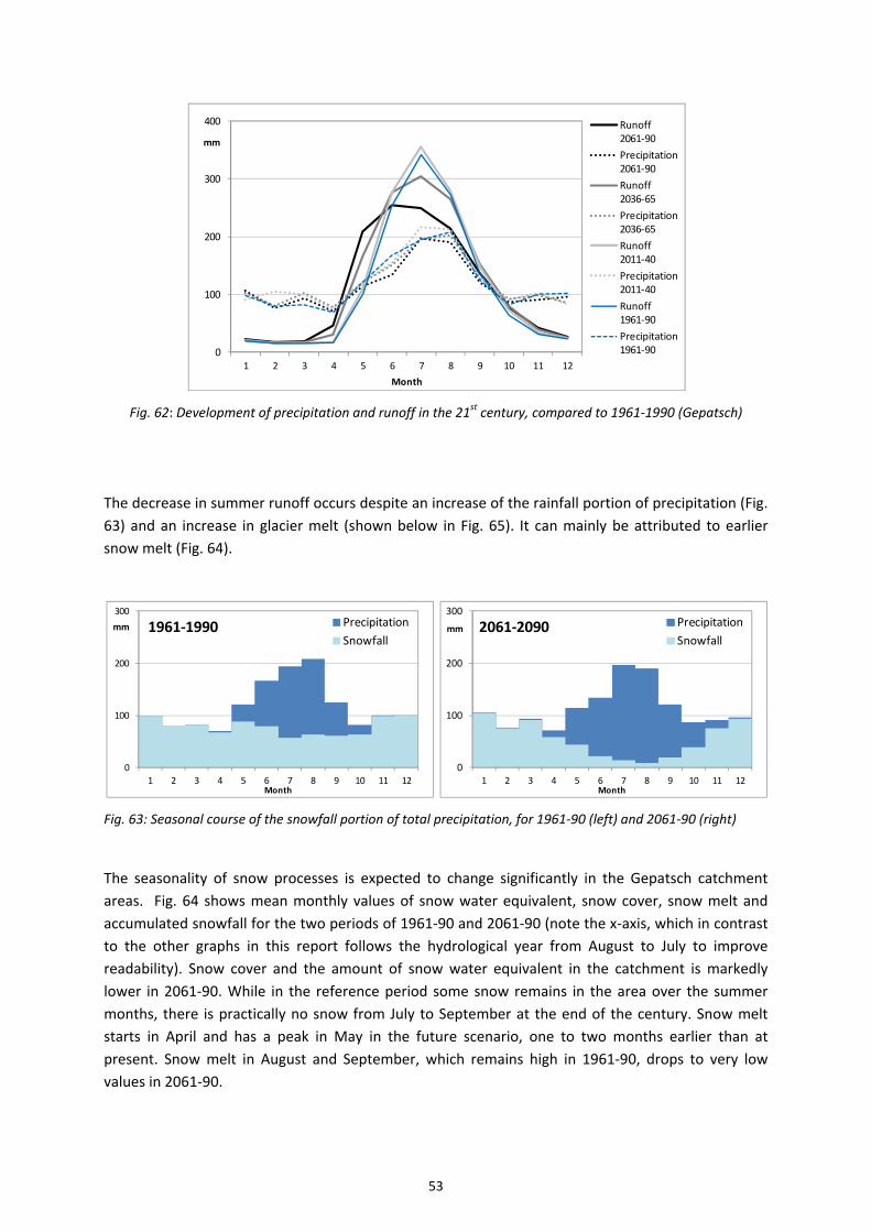
53

Fig. 62: Development of precipitation and runoff in the 21st century, compared to 1961‐1990 (Gepatsch)

The decrease in summer runoff occurs despite an increase of the rainfall portion of precipitation (Fig.

63) and an increase in glacier melt (shown below in Fig. 65). It can mainly be attributed to earlier

snow melt (Fig. 64).

Fig. 63: Seasonal course of the snowfall portion of total precipitation, for 1961‐90 (left) and 2061‐90 (right)

The seasonality of snow processes is expected to change significantly in the Gepatsch catchment

areas. Fig. 64 shows mean monthly values of snow water equivalent, snow cover, snow melt and

accumulated snowfall for the two periods of 1961‐90 and 2061‐90 (note the x‐axis, which in contrast

to the other graphs in this report follows the hydrological year from August to July to improve

readability). Snow cover and the amount of snow water equivalent in the catchment is markedly

lower in 2061‐90. While in the reference period some snow remains in the area over the summer

months, there is practically no snow from July to September at the end of the century. Snow melt

starts in April and has a peak in May in the future scenario, one to two months earlier than at

present. Snow melt in August and September, which remains high in 1961‐90, drops to very low

values in 2061‐90.

0

100

200

300

400

1 2 3 4 5 6 7 8 9 10 11 12

mm

Month

Runoff 2061‐90

Precipitation 2061‐90

Runoff 2036‐65


Runoff 2011‐40


Runoff 1961‐90


0

100

200

300

1 2 3 4 5 6 7 8 9 10 11 12

mm

Month

1961‐1990 Precipitation

Snowfall

0

100

200

300

1 2 3 4 5 6 7 8 9 10 11 12

mm

Month

2061‐2090 Precipitation

Snowfall

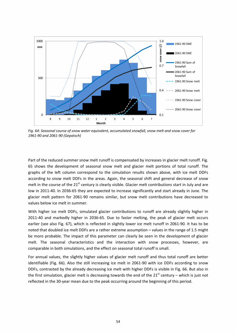
54

Fig. 64: Seasonal course of snow water equivalent, accumulated snowfall, snow melt and snow cover for 1961‐90 and 2061‐90 (Gepatsch)

Part of the reduced summer snow melt runoff is compensated by increases in glacier melt runoff. Fig.

65 shows the development of seasonal snow melt and glacier melt portions of total runoff. The

graphs of the left column correspond to the simulation results shown above, with ice melt DDFs

according to snow melt DDFs in the areas. Again, the seasonal shift and general decrease of snow

melt in the course of the 21st century is clearly visible. Glacier melt contributions start in July and are

low in 2011‐40. In 2036‐65 they are expected to increase significantly and start already in June. The

glacier melt pattern for 2061‐90 remains similar, but snow melt contributions have decreased to

values below ice melt in summer.

With higher ice melt DDFs, simulated glacier contributions to runoff are already slightly higher in

2011‐40 and markedly higher in 2036‐65. Due to faster melting, the peak of glacier melt occurs

earlier (see also Fig. 67), which is reflected in slightly lower ice melt runoff in 2061‐90. It has to be

noted that doubled ice melt DDFs are a rather extreme assumption – values in the range of 1.5 might

be more probable. The impact of this parameter can clearly be seen in the development of glacier

melt. The seasonal characteristics and the interaction with snow processes, however, are

comparable in both simulations, and the effect on seasonal total runoff is small.

For annual values, the slightly higher values of glacier melt runoff and thus total runoff are better

identifiable (Fig. 66). Also the still increasing ice melt in 2061‐90 with ice DDFs according to snow

DDFs, contrasted by the already decreasing ice melt with higher DDFs is visible in Fig. 66. But also in

the first simulation, glacier melt is decreasing towards the end of the 21st century – which is just not

reflected in the 30‐year mean due to the peak occurring around the beginning of this period.

0.1

0.4

0.7

1.0

0

500

1000

8 9 10 11 12 1 2 3 4 5 6 7

Month

snow cover (/)

mm1961‐90 SWE

2061‐90 SWE

1961‐90 Sum of Snowfall


1961‐90 Snow melt

2061‐90 Snow melt

1961‐90 Snow cover


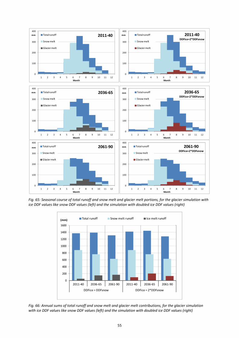
55

Fig. 65: Seasonal course of total runoff and snow melt and glacier melt portions, for the glacier simulation with ice DDF values like snow DDF values (left) and the simulation with doubled ice DDF values (right)

Fig. 66: Annual sums of total runoff and snow melt and glacier melt contributions, for the glacier simulation with ice DDF values like snow DDF values (left) and the simulation with doubled ice DDF values (right)

0

100

200

300

400

1 2 3 4 5 6 7 8 9 10 11 12

mm

Month

2011‐40Total runoff

Snow melt

Glacier melt

0

100

200

300

400

1 2 3 4 5 6 7 8 9 10 11 12

mm

Month

2011‐40DDFice=2*DDFsnow

Total runoff

Snow melt

Glacier melt

0

100

200

300

400

1 2 3 4 5 6 7 8 9 10 11 12

mm

Month


Snow melt

Glacier melt

0

100

200

300

400

1 2 3 4 5 6 7 8 9 10 11 12

mm

Month


Total runoff

Snow melt

Glacier melt

0

100

200

300

400

1 2 3 4 5 6 7 8 9 10 11 12

mm

Month


Snow melt

Glacier melt

0

100

200

300

400

1 2 3 4 5 6 7 8 9 10 11 12

mm

Month


Total runoff

Snow melt

Glacier melt

0

200

400

600

800

1000

1200

1400

1600

2011‐40 2036‐65 2061‐90 2011‐40 2036‐65 2061‐90

DDFice = DDFsnow DDFice = 2*DDFsnow

(mm) Total runoff Snow melt runoff Ice melt runoff

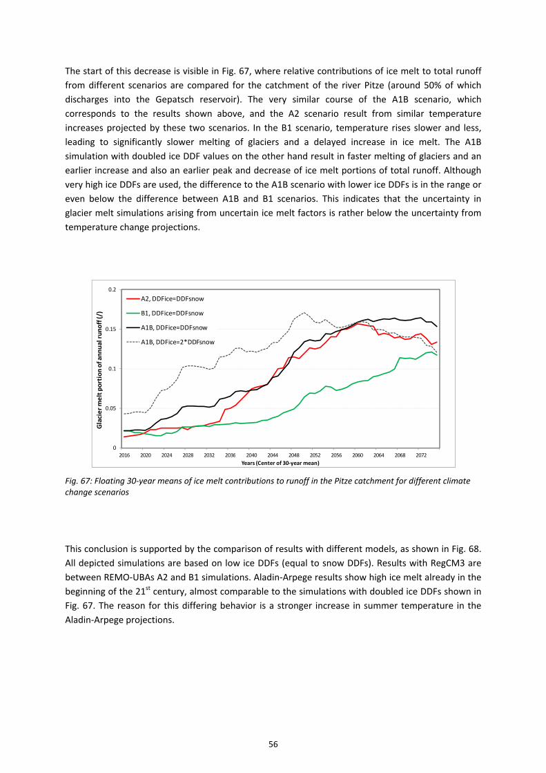
56

The start of this decrease is visible in Fig. 67, where relative contributions of ice melt to total runoff

from different scenarios are compared for the catchment of the river Pitze (around 50% of which

discharges into the Gepatsch reservoir). The very similar course of the A1B scenario, which

corresponds to the results shown above, and the A2 scenario result from similar temperature

increases projected by these two scenarios. In the B1 scenario, temperature rises slower and less,

leading to significantly slower melting of glaciers and a delayed increase in ice melt. The A1B

simulation with doubled ice DDF values on the other hand result in faster melting of glaciers and an

earlier increase and also an earlier peak and decrease of ice melt portions of total runoff. Although

very high ice DDFs are used, the difference to the A1B scenario with lower ice DDFs is in the range or

even below the difference between A1B and B1 scenarios. This indicates that the uncertainty in

glacier melt simulations arising from uncertain ice melt factors is rather below the uncertainty from

temperature change projections.

Fig. 67: Floating 30‐year means of ice melt contributions to runoff in the Pitze catchment for different climate change scenarios

This conclusion is supported by the comparison of results with different models, as shown in Fig. 68.

All depicted simulations are based on low ice DDFs (equal to snow DDFs). Results with RegCM3 are

between REMO‐UBAs A2 and B1 simulations. Aladin‐Arpege results show high ice melt already in the

beginning of the 21st century, almost comparable to the simulations with doubled ice DDFs shown in

Fig. 67. The reason for this differing behavior is a stronger increase in summer temperature in the

Aladin‐Arpege projections.

0

0.05

0.1

0.15

0.2

2016 2020 2024 2028 2032 2036 2040 2044 2048 2052 2056 2060 2064 2068 2072

Glacier melt portion of annual runoff (/)

Years (Center of 30‐year mean)

A2, DDFice=DDFsnow

B1, DDFice=DDFsnow

A1B, DDFice=DDFsnow

A1B, DDFice=2*DDFsnow

57

Fig. 68: Floating 30‐year means of ice melt contributions to runoff in the Pitze catchment simulated with climate data of different models and different emission scenarios

The drastic loss of glacier volumes corresponding to the shown increases in ice melt runoff is shown

in Fig. 69, again for the A1B scenario and both ice melt DDF assumptions. This graph, like the

analyses before, refers to 30‐year means and sums over the entire Gepatsch catchment. Fig. 70

shows the spatial distribution of simulated ice water equivalents and refers to snapshots for specific

years. Therefore, also the very last simulated year, 2090, can be shown. This reveals that, based on

very high ice DDF values, the melting of all glaciers in the Gepatsch area is almost completed in 2090

(Fig. 70, bottom right). Assuming low ice DDFs, substantial areas with glaciers remain in 2090, but

with very low volumes (Fig. 70, bottom left).

Fig. 69: Development of simulated ice water equivalent in the cachment areas of the Gepatsch reservoir in the 21st century, with ice DDF values like snow DDF values (left) and doubled ice DDF values (right)

0

0.05

0.1

0.15

0.2

2016 2020 2024 2028 2032 2036 2040 2044 2048 2052 2056 2060 2064 2068 2072

Glacier melt portion of annual runoff (/)

Years (Center of 30‐year mean)

Pitze

REMO‐UBA A2

REMO‐UBA B1

REMO‐UBA A1B

ARPEGE A1B

RegCM3 A1B

0

500

1000

1500

2000

2500

3000

DDFice = DDFsnow DDFice = 2*DDFsnow

Ice water equivalent (M

io. m³)

Start value 2000 Mean 2011‐40 Mean 2036‐65 Mean 2061‐90

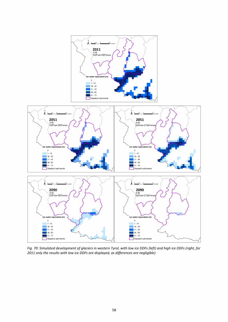
58

Fig. 70: Simulated development of glaciers in western Tyrol, with low ice DDFs (left) and high ice DDFs (right, for 2011 only the results with low ice DDFs are displayed, as differences are negligible)

59

4.5.2. Sellrain‐Silz

In the catchment areas of the Sellrain‐Silz hydropower system, the decrease in summer runoff is

especially pronounced (Fig. 71). This strong decrease is caused by a significant decrease in summer

precipitation that is more pronounced than in the other two analysed areas. Additionally, the

Sellrain‐Silz catchments have smaller glacierized portions. This means that the decrease in snow melt

runoff in summer months, which is shown in Fig. 72, is less compensated by ice melt runoff. The

general pattern of lower summer and higher spring runoff, with an earlier peak (Fig. 71), is

comparable to the development in the other reservoir catchment areas. Also, overall decrease of

accumulated snow water equivalent and seasonal changes in snow cover and snow melt (Fig. 72) are

similar to the changes in the other investigated areas.

Fig. 71: Development of precipitation and runoff in the 21st century, compared to 1961‐1990 (Sellrain‐Silz)

Fig. 72: Seasonal course of snow water equivalent, accumulated snowfall, snow melt and snow cover for 1961‐90 and 2061‐90 (Sellrain‐Silz)

0

100

200

300

400

500

600

1 2 3 4 5 6 7 8 9 10 11 12

mm

Month

Runoff 2061‐90


Runoff 2036‐65


Runoff 2011‐40


Runoff 1961‐90


0.1

0.4

0.7

1.0

0

500

1000

1500

8 9 10 11 12 1 2 3 4 5 6 7

Monat

snow cover (/)mm

1961‐90 SWE

2061‐90 SWE



1961‐90 Snow melt

2061‐90 Snow melt



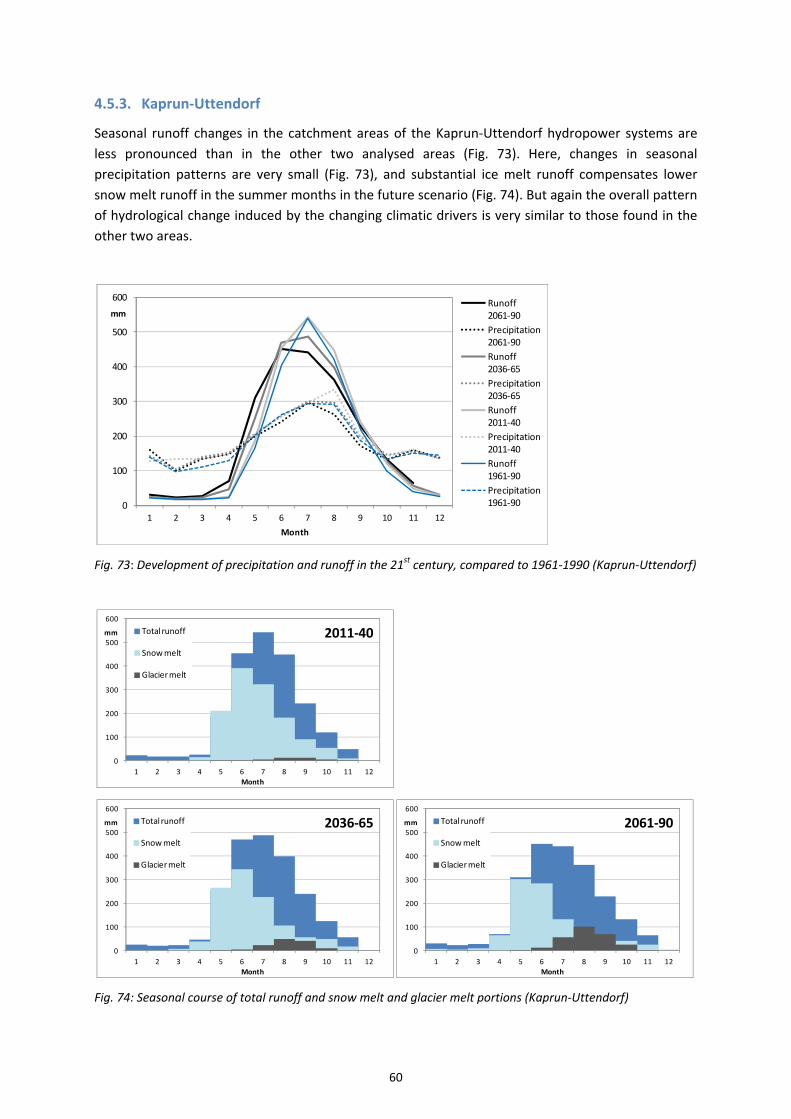
60

4.5.3. Kaprun‐Uttendorf

Seasonal runoff changes in the catchment areas of the Kaprun‐Uttendorf hydropower systems are

less pronounced than in the other two analysed areas (Fig. 73). Here, changes in seasonal

precipitation patterns are very small (Fig. 73), and substantial ice melt runoff compensates lower

snow melt runoff in the summer months in the future scenario (Fig. 74). But again the overall pattern

of hydrological change induced by the changing climatic drivers is very similar to those found in the

other two areas.

Fig. 73: Development of precipitation and runoff in the 21st century, compared to 1961‐1990 (Kaprun‐Uttendorf)

Fig. 74: Seasonal course of total runoff and snow melt and glacier melt portions (Kaprun‐Uttendorf)

0

100

200

300

400

500

600

1 2 3 4 5 6 7 8 9 10 11 12

mm

Month

Runoff 2061‐90


Runoff 2036‐65


Runoff 2011‐40


Runoff 1961‐90


0

100

200

300

400

500

600

1 2 3 4 5 6 7 8 9 10 11 12

mm

Month


Snow melt

Glacier melt

0

100

200

300

400

500

600

1 2 3 4 5 6 7 8 9 10 11 12

mm

Month


Snow melt

Glacier melt

0

100

200

300

400

500

600

1 2 3 4 5 6 7 8 9 10 11 12

mm

Month


Snow melt

Glacier melt

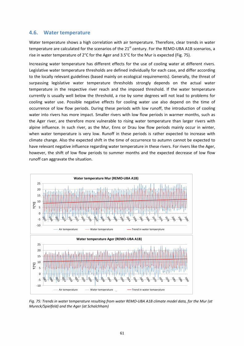
61

4.6. Water temperature

Water temperature shows a high correlation with air temperature. Therefore, clear trends in water

temperature are calculated for the scenarios of the 21st century. For the REMO‐UBA A1B scenarios, a

rise in water temperature of 2°C for the Ager and 3.5°C for the Mur is expected (Fig. 75).

Increasing water temperature has different effects for the use of cooling water at different rivers.

Legislative water temperature thresholds are defined individually for each case, and differ according

to the locally relevant guidelines (based mainly on ecological requirements). Generally, the threat of

surpassing legislative water temperature thresholds strongly depends on the actual water

temperature in the respective river reach and the imposed threshold. If the water temperature

currently is usually well below the threshold, a rise by some degrees will not lead to problems for

cooling water use. Possible negative effects for cooling water use also depend on the time of

occurrence of low flow periods. During these periods with low runoff, the introduction of cooling

water into rivers has more impact. Smaller rivers with low flow periods in warmer months, such as

the Ager river, are therefore more vulnerable to rising water temperature than larger rivers with

alpine influence. In such river, as the Mur, Enns or Drau low flow periods mainly occur in winter,

when water temperature is very low. Runoff in these periods is rather expected to increase with

climate change. Also the expected shift in the time of occurrence to autumn cannot be expected to

have relevant negative influence regarding water temperature in these rivers. For rivers like the Ager,

however, the shift of low flow periods to summer months and the expected decrease of low flow

runoff can aggravate the situation.

Fig. 75: Trends in water temperature resulting from water REMO‐UBA A1B climate model data, for the Mur (at Mureck/Spielfeld) and the Ager (at Schalchham)

‐10

‐5

0

5

10

15

20

25

T [°C]

Mur ‐ Temperaturentwicklung A1B Szenario

Lufttemperatur Wassertemperatur Mur Trend der Wassertemperatur

‐10

‐5

0

5

10

15

20

25

T [°C]

Ager ‐ Temperaturentwicklung A1B Szenario

Lufttemperatur Wassertemperatur Ager Trend der Wassertemperatur

Water temperature Mur (REMO‐UBA A1B)

Water temperature Ager (REMO‐UBA A1B)

Water temperatureAir temperature Trend in water temperature

Water temperatureAir temperature Trend in water temperature

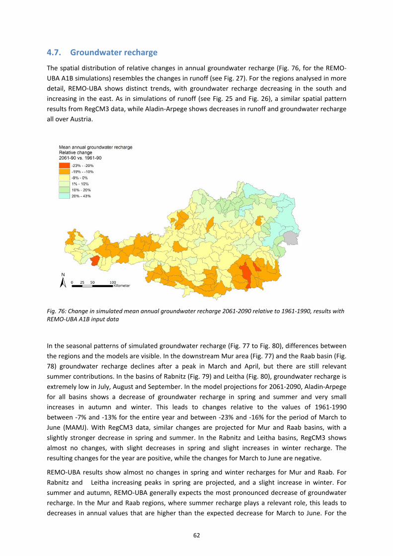
62

4.7. Groundwater recharge

The spatial distribution of relative changes in annual groundwater recharge (Fig. 76, for the REMO‐

UBA A1B simulations) resembles the changes in runoff (see Fig. 27). For the regions analysed in more

detail, REMO‐UBA shows distinct trends, with groundwater recharge decreasing in the south and

increasing in the east. As in simulations of runoff (see Fig. 25 and Fig. 26), a similar spatial pattern

results from RegCM3 data, while Aladin‐Arpege shows decreases in runoff and groundwater recharge

all over Austria.

Fig. 76: Change in simulated mean annual groundwater recharge 2061‐2090 relative to 1961‐1990, results with REMO‐UBA A1B input data

In the seasonal patterns of simulated groundwater recharge (Fig. 77 to Fig. 80), differences between

the regions and the models are visible. In the downstream Mur area (Fig. 77) and the Raab basin (Fig.

78) groundwater recharge declines after a peak in March and April, but there are still relevant

summer contributions. In the basins of Rabnitz (Fig. 79) and Leitha (Fig. 80), groundwater recharge is

extremely low in July, August and September. In the model projections for 2061‐2090, Aladin‐Arpege

for all basins shows a decrease of groundwater recharge in spring and summer and very small

increases in autumn and winter. This leads to changes relative to the values of 1961‐1990

between ‐7% and ‐13% for the entire year and between ‐23% and ‐16% for the period of March to

June (MAMJ). With RegCM3 data, similar changes are projected for Mur and Raab basins, with a

slightly stronger decrease in spring and summer. In the Rabnitz and Leitha basins, RegCM3 shows

almost no changes, with slight decreases in spring and slight increases in winter recharge. The

resulting changes for the year are positive, while the changes for March to June are negative.

REMO‐UBA results show almost no changes in spring and winter recharges for Mur and Raab. For

Rabnitz and Leitha increasing peaks in spring are projected, and a slight increase in winter. For

summer and autumn, REMO‐UBA generally expects the most pronounced decrease of groundwater

recharge. In the Mur and Raab regions, where summer recharge plays a relevant role, this leads to

decreases in annual values that are higher than the expected decrease for March to June. For the

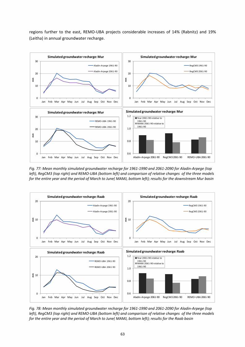
63

regions further to the east, REMO‐UBA projects considerable increases of 14% (Rabnitz) and 19%

(Leitha) in annual groundwater recharge.

Fig. 77: Mean monthly simulated groundwater recharge for 1961‐1990 and 2061‐2090 for Aladin‐Arpege (top left), RegCM3 (top right) and REMO‐UBA (bottom left) and comparison of relative changes of the three models for the entire year and the period of March to June( MAMJ, bottom left); results for the downstream Mur basin

Fig. 78: Mean monthly simulated groundwater recharge for 1961‐1990 and 2061‐2090 for Aladin‐Arpege (top left), RegCM3 (top right) and REMO‐UBA (bottom left) and comparison of relative changes of the three models for the entire year and the period of March to June( MAMJ, bottom left); results for the Raab basin

0

10

20

30

Jan Feb Mar Apr May Jun Jul Aug Sep Oct Nov Dec

mm

Simulated groundwater recharge: Mur



0

10

20

30


mm


RegCM3 1961‐90

RegCM3 2061‐90

0

10

20

30


mm


REMO‐UBA 1961‐90


0.6

0.8

1.0

1.2

Aladin‐Arpege 2061‐90 RegCM3 2061‐90 REMO‐UBA 2061‐90


Year 2061‐90 relative to 1961‐90MAMJ 2061‐90 relative to 1961‐90

0

10

20


mm

Simulated groundwater recharge: Raab



0

10

20


mm


RegCM3 1961‐90

RegCM3 2061‐90

0

10

20


mm




0.6

0.8

1.0

1.2




64

Fig. 79: Mean monthly simulated groundwater recharge for 1961‐1990 and 2061‐2090 for Aladin‐Arpege (top left), RegCM3 (top right) and REMO‐UBA (bottom left) and comparison of relative changes of the three models for the entire year and the period of March to June( MAMJ, bottom left); results for the Rabnitz basin

Fig. 80: Mean monthly simulated groundwater recharge for 1961‐1990 and 2061‐2090 for Aladin‐Arpege (top left), RegCM3 (top right) and REMO‐UBA (bottom left) and comparison of relative changes of the three models for the entire year and the period of March to June( MAMJ, bottom left); results for the Leitha basin

0

10

20


mm

Simulated groundwater recharge: Rabnitz



0

10

20


mm


RegCM3 1961‐90

RegCM3 2061‐90

0

10

20


mm




0.6

0.8

1.0

1.2




0

10

20


mm

Simulated groundwater recharge: Leitha



0

10

20


mm


RegCM3 1961‐90

RegCM3 2061‐90

0

10

20

30


mm




0.6

0.8

1.0

1.2

1.4




65

4.8. Trends in runoff and hydropower production in Europe

4.8.1. Mean runoff and hydropower potential

Based on an application of the WaterGAP model, runoff trends and their implications for hydropower

generation are analysed by Lehner et al. (2005). In a comparison of several large scale hydrological

and land surface models, the WaterGAP model recently achieved the best representation of seasonal

runoff trends (Stahl et al. 2011). The global hydrological model WaterGAP is driven by precipitation

and temperature input data from two GCMs, ECHAM4 and HADCM3. The hydrological model also

includes scenarios on human water use and management. The greenhouse gas emission scenario

applied is similar to the widely used IPCC A1B scenario. The analysed time periods are the decade of

the 2020s and the 2070s, and the reference period of 1961‐1990.

Resulting from an overall decrease in runoff, the gross hydropower potential is projected to decrease

by about 6% by the 2070s, with large regional variability (Lehner et al. 2005). The spatial pattern of

simulated runoff trends due to climate change projections is shown in Figure 1. For the 2020s, the

differences between the two climate models are immense (different signs in Spain and almost the

entire northern part of Europe). The large discrepancies can probably be explained by the larger

influence of the – random – model “weather” relative to the climate change signal. For the 2070s

with their stronger climate change signal, the patterns are similar, with a general decrease of runoff

south of the Alps and an increase north. With both models, Austria is located at the transition of

increasing and decreasing trends, with HADCM3 showing mostly a decrease and ECHAM4 no relevant

change. Calculated with HADCM3 results, the gross hydropower potential for Austria decreases by

15.9 to 17.5% by the 2070s (Table1, depending on the calculation method). In addition to the gross

hydropower potential, which is based only on discharge and elevation, the developed hydropower

potential was analysed by Lehner et al. (2005). For this value, the discharge at main reservoir and

run‐of‐river stations was considered, assuming a constant level of hydropower development. For the

developed hydropower potential, results for both models are presented countrywise (Table 1). For

Austria and the 2070s, a similar value of decrease results for the HADCM3 model (‐13.1%), while the

results with the ECHAM4 model show practically no change (+1.3%), which is consistent with the

projection of unchanged runoff in Fig. 1.

The results for Austria and the 2070s can be compared to the results of the KlimAdapt project (Kranzl

et al. 2010, Stanzel and Nachtnebel 2010) for the period of 2061‐2090 and the A1B scenario. In

KlimAdapt, hydropower production was deducted from the weighted gross hydropower potential,

with weights according to actual production. Therefore it corresponds rather to the developed

hydropower potential of Lehner et al. (2005). The projected decrease of 15% between 2025 and 2075

in KlimAdapt is very close to their results of ‐13% with the HADCM3 model. Gross hydropower

potential was calculated to decrease by 10% in KlimAdapt, which is lower than the ‐16 to ‐17% of

Lehner et al. (2005). The differences can be attributed to different spatial patterns in input variables,

especially precipitation. Also different topographic information on the larger scale (0.5°, as opposed

to 1km in KlimAdapt) can contribute to differences in resulting gross hydropower potential. The

value for the 1961‐90 gross hydropower potential in Lehner et al. (2005) of 150 or 160 TWh/a is

similar to that calculated by Pöyry (2008) and slightly higher than that estimated in KlimAdapt, where

south‐eastern Austria was excluded. As especially in the Austrian south‐east runoff is expected to

decrease (in both, KlimAdapts REMO‐UBA model and the HADCM3 model, see Fig. 1.), also this

different coverage of the area of Austria might add to the differences in the projections of gross

hydropower potential.

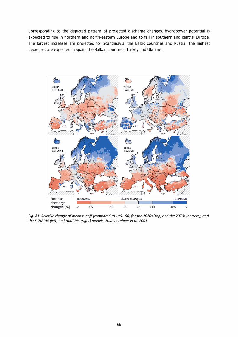
66

Corresponding to the depicted pattern of projected discharge changes, hydropower potential is

expected to rise in northern and north‐eastern Europe and to fall in southern and central Europe.

The largest increases are projected for Scandinavia, the Baltic countries and Russia. The highest

decreases are expected in Spain, the Balkan countries, Turkey and Ukraine.

Fig. 81: Relative change of mean runoff (compared to 1961‐90) for the 2020s (top) and the 2070s (bottom), and the ECHAM4 (left) and HadCM3 (right) models. Source: Lehner et al. 2005

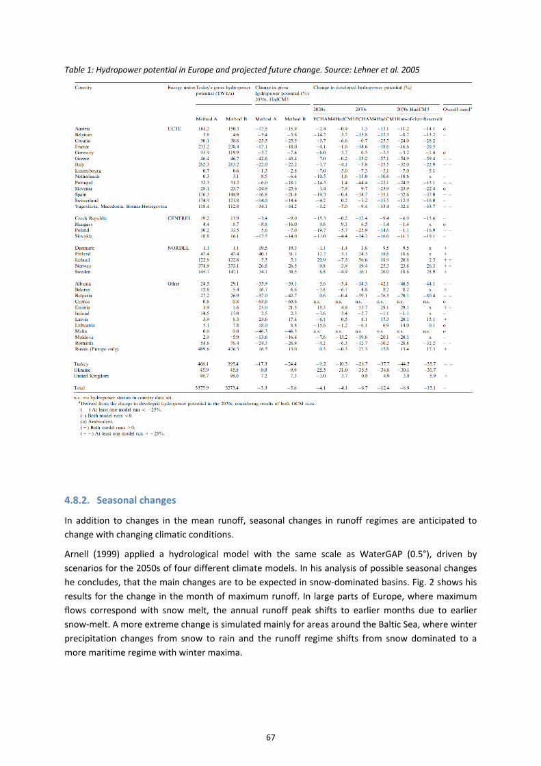
67

Table 1: Hydropower potential in Europe and projected future change. Source: Lehner et al. 2005

4.8.2. Seasonal changes

In addition to changes in the mean runoff, seasonal changes in runoff regimes are anticipated to

change with changing climatic conditions.

Arnell (1999) applied a hydrological model with the same scale as WaterGAP (0.5°), driven by

scenarios for the 2050s of four different climate models. In his analysis of possible seasonal changes

he concludes, that the main changes are to be expected in snow‐dominated basins. Fig. 2 shows his

results for the change in the month of maximum runoff. In large parts of Europe, where maximum

flows correspond with snow melt, the annual runoff peak shifts to earlier months due to earlier

snow‐melt. A more extreme change is simulated mainly for areas around the Baltic Sea, where winter

precipitation changes from snow to rain and the runoff regime shifts from snow dominated to a

more maritime regime with winter maxima.

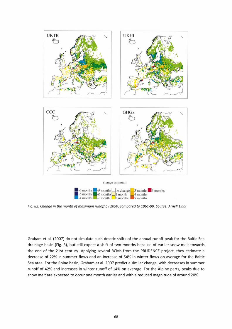
68

Fig. 82: Change in the month of maximum runoff by 2050, compared to 1961‐90. Source: Arnell 1999

Graham et al. (2007) do not simulate such drastic shifts of the annual runoff peak for the Baltic Sea

drainage basin (Fig. 3), but still expect a shift of two months because of earlier snow‐melt towards

the end of the 21st century. Applying several RCMs from the PRUDENCE project, they estimate a

decrease of 22% in summer flows and an increase of 54% in winter flows on average for the Baltic

Sea area. For the Rhine basin, Graham et al. 2007 predict a similar change, with decreases in summer

runoff of 42% and increases in winter runoff of 14% on average. For the Alpine parts, peaks due to

snow melt are expected to occur one month earlier and with a reduced magnitude of around 20%.

69

Fig. 83: Change in seasonal runoff to the Baltic Sea, 2071‐2100 compared to 1961‐90, in 2 B2 scenarios (left) and 3 A2 scenarios (right). Source: Graham et al. 2007

Middelkoop et al. (2001) come to analog results in their hydrological modeling study of the Rhine

basin, using UKHI and CCC climate model scenarios for 2050 (like Arnell, 1999, see above): “Due to

climate change the river Rhine is expected to shift from a combined rainfall‐snowmelt regime to a

more rainfall dominated regime. This coincides with a seasonal change in the discharge regime:

winter discharge will increase, and summer discharges decrease.” For middle‐mountain areas they

expect the least seasonal changes in runoff.

For the Elbe basin, with a major influence from middle‐mountain areas, this is also shown by

Hattermann et al. (2008). While they do not expect major seasonal changes in their application with

an ECHAM4 A1 scenario, they also come to the conclusion that by 2050 there will be less water

available in summer and that the high flow period due to snow melt will occur earlier in the year.

For the Danube basin, which has a stronger Alpine influence, a more pronounced change in runoff

seasonality, as in the Rhine basin, is projected by Kling et al. (2012). Their simulation results for

2071‐2100 with all 23 RCMs from the ENSEMBLES project show a considerable decrease of summer

runoff, a moderate increase of winter runoff and the occurrence of the annual runoff peak one to

two months earlier. These results correspond with those for the major Austrian Danube tributaries in

KlimAdapt (Stanzel and Nachtnebel 2010), who furthermore show that the seasonal changes in

runoff are more pronounced with a higher relevance of snow processes.

For the Ebro basin, Zambrano‐Bigiarini et al. (2011) use two PRUDENCE RCMs and expect a reduction

of mean runoff throughout the year for 2071‐2100, with especially strong decreases in winter.

The outlined projected changes are already observable in runoff measurements, as shown by Stahl et

al. (2010), who analysed trends in a large dataset of 1962‐2004 streamflow data from basins with no

direct human influence. They found predominant positive trends in winter runoff, with exceptions of

decreasing flow in Spain, Southern France, South‐east Austria, Czech Republic and Slovakia. For Italy

and South‐east Europe, no observations were included in the analysis. For the months from April to

August, negative trends were detected almost everywhere in Europe, with some exceptions in

Scandinavia and the UK.

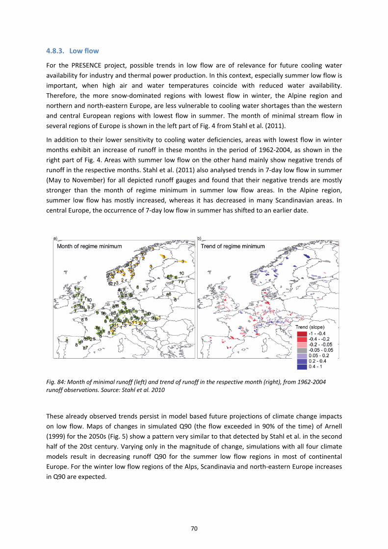
70

4.8.3. Low flow

For the PRESENCE project, possible trends in low flow are of relevance for future cooling water

availability for industry and thermal power production. In this context, especially summer low flow is

important, when high air and water temperatures coincide with reduced water availability.

Therefore, the more snow‐dominated regions with lowest flow in winter, the Alpine region and

northern and north‐eastern Europe, are less vulnerable to cooling water shortages than the western

and central European regions with lowest flow in summer. The month of minimal stream flow in

several regions of Europe is shown in the left part of Fig. 4 from Stahl et al. (2011).

In addition to their lower sensitivity to cooling water deficiencies, areas with lowest flow in winter

months exhibit an increase of runoff in these months in the period of 1962‐2004, as shown in the

right part of Fig. 4. Areas with summer low flow on the other hand mainly show negative trends of

runoff in the respective months. Stahl et al. (2011) also analysed trends in 7‐day low flow in summer

(May to November) for all depicted runoff gauges and found that their negative trends are mostly

stronger than the month of regime minimum in summer low flow areas. In the Alpine region,

summer low flow has mostly increased, whereas it has decreased in many Scandinavian areas. In

central Europe, the occurrence of 7‐day low flow in summer has shifted to an earlier date.

Fig. 84: Month of minimal runoff (left) and trend of runoff in the respective month (right), from 1962‐2004 runoff observations. Source: Stahl et al. 2010

These already observed trends persist in model based future projections of climate change impacts

on low flow. Maps of changes in simulated Q90 (the flow exceeded in 90% of the time) of Arnell

(1999) for the 2050s (Fig. 5) show a pattern very similar to that detected by Stahl et al. in the second

half of the 20st century. Varying only in the magnitude of change, simulations with all four climate

models result in decreasing runoff Q90 for the summer low flow regions in most of continental

Europe. For the winter low flow regions of the Alps, Scandinavia and north‐eastern Europe increases

in Q90 are expected.

71

Fig. 85: Change in the flow exceeded 90% of the time (Q90) by 2050, compared to 1961‐90. Source: Arnell 1999

Also Lehner et al. (2006) come to corresponding results in the analysis of runoff extreme of their

WaterGAP application with climate model input data. Fig. 6 shows the return period of the actual

100‐year low flow events in the simulations for the 2070s. Again, for most of Europe, except the

snow‐dominated Alpine and northern European regions, an aggravation of the low flow water

availability is expected, as today’s drought runoff level is projected to be reached more frequently.

Discrepancies of Lehner et al.’s projections and those of Arnell (1999) for Germany and parts of

eastern Europe might be attributed to water use scenarios assumed by Lehner et al. (2006), as they

expect a decrease in drought intensity only from changed water use in Germany, and a substantial

increase in eastern Europe.

72

Fig. 86: Change in recurrence of today’s 100‐year droughts (1961‐90) by the 2070s. Source: Lehner et al. 2006

73

5. Conclusions

In this report, the impact of climate change on hydrology is investigated with a special focus on the

effects for hydropower production and cooling water availability. The assessment is based on water

balance simulations for Austria, using climate model scenarios as input data. Scenario data from

three different RCMs, REMO‐UBA, Aladin‐Arpege and RegCM3 are applied.

The relation between changes in long term mean annual runoff and changes in long term means of

precipitation and temperature, also termed runoff elasticity, is assessed for 188 Austrian catchments.

A multiple linear regression model can be fitted very well to simulation results of the water balance

model driven by three different scenarios of the REMO‐UBA model. Results can be improved by

grouping the catchments into alpine and lowland areas and fitting two regression models. For further

analysis, the results from water balance simulations with different climate model input are used

directly, and the regression model is not applied.

Spatial patterns of changes in runoff induced by climate change differ according to the applied

climate model. REMO‐UBA and RegCM3, which are driven by the same GCM, lead to hydrological

scenarios with decreasing runoff in the south and west of Austria and small increases in the north‐

east. Aladin‐Arpege scenarios result in decreasing runoff all over Austria, but more pronounced in

the south and west.

Simulated runoff time series are analysed for the rivers Enns, Mur and Drau. Several run‐of‐river

hydropower plants are located along these rivers and substantial discharge from thermal power

plants and industry is expected. Results from the river Ager are shown to investigate the situation for

smaller rivers with less alpine influence.

In simulations with the REMO‐UBA model, mean runoff differs according to the greenhouse gas

emission scenario. The A2 scenario, with higher precipitation, leads to higher runoff than the drier

A1B scenario. Both scenarios show a decreasing trend within the 21st century. Similar trends are

simulated by the other two models (both only with A1B scenarios). Stronger decreases are projected

by Aladin‐Arpege. The expected changes are very similar along the entire Austrian reaches of Enns,

Mur and Drau. The simulated decrease in mean runoff until the period of 2061‐2090 is around 10%,

which does not indicate general shortages of cooling water, but results in an overall reduction of

hydropower production.

Seasonal changes are simulated consistently between models, scenarios and basins, with runoff

increases in winter and spring and decreases in summer and fall. The summer runoff decrease is

more severe in the scenario A1B. Increases in winter runoff are less pronounced in the simulations

with Aladin‐Arpege. With earlier and less snow melt, the peak of seasonal runoff in Enns, Mur and

Drau is expected to be lower and occur one month earlier. This change is more pronounced in alpine

upstream catchments with stronger influence of snow processes. For the Ager, the projections for

changes in the seasonal peak in early spring differ between the models. The trend towards a less

pronounced runoff seasonality in all rivers with Alpine influence has positive effects for hydropower

production, as the divergence between production and demand diminishes.

In the rivers Enns, Mur and Drau low flow occurs mainly in winter. Increasing winter runoff therefore

leads to increasing low flow runoff. This increase in low flow discharge is projected consistently by

RegCM3 and both REMO‐UBA emission scenarios. Simulations with Aladin‐Arpege do not show

relevant changes in low flow runoff for these three rivers. For the Ager, all models expect significant

reductions in low flow runoff.

74

Low flow periods are expected to partly shift to earlier months, from winter to autumn for Enns, Mur

and Drau, from autumn to summer for the Ager. For the Ager and similar rivers, the more frequent

occurrence of low flow periods in summer together with increasing water temperature can have

negative effects for cooling water use. Concerning the duration of low flow periods, no clear

conclusions can be drawn from the conducted analyses.

Long‐term persistence and periodicity in runoff time series is more pronounced in simulations for the

second half of the 21st century with A1B emission scenarios than under reference conditions. This

effect is small in simulations driven by RegCM3 and Aladin‐Arpege, but considerable in REMO‐UBA

results. This weak coincidence and the fact that persistence in simulations with climate model control

run data and with observations is similar might indicate that longer periods of persistent runoff can

be expected under climate change conditions. With A2 data, however, no such change in persistence

behavior is detected.

Changes in groundwater recharge show spatial patterns similar to those of changes in runoff. For the

south of Austria, scenario simulations with all models consistently show decreasing groundwater

recharge. For the east, the sign of the expected change depends on the applied model, with

REMO‐UBA showing increases, Aladin‐Arpege decreases and RegCM3 no relevant changes.

Inflow into alpine reservoirs is assessed for three reservoir systems. While inflow in summer

decreases under climate change conditions, spring inflow increases. The peak in monthly runoff is

less pronounced and occurs one month earlier. The main cause for this is that snow melt starts

earlier, which leads to higher snow melt runoff in spring, and also ends earlier, which leads to less

snow melt contributions in summer. More ice melt runoff from glacierized areas in summer months

partly compensates the decreasing snow melt contributions. Towards the end of the 21st century, ice

melt runoff decreases again, due to the advanced loss of glacier ice volumes. The projected changes

in high alpine areas are triggered by temperature change to a high extent and are therefore subject

to less uncertainty than changes driven by precipitation changes. Especially glacier development,

however, is also highly sensitive to the (smaller) differences in temperature projections.

A literature review of possible changes in runoff and hydropower production in Europe shows

expected increases in northern and north‐eastern Europe, especially in Scandinavia, the Baltic

countries and Russia. Decreases are expected in southern and central Europe, notably in Spain, the

Balkan countries, Turkey and Ukraine. A more balanced seasonal course of runoff and power

production is generally expected, with streamflow increasing in winter and decreasing in summer. In

southern Europe, as e.g. in the Ebro basin, general decreases of streamflow throughout the year can

be expected. Seasonal changes are more pronounced in regions with stronger influence of snow

processes, as in the Alps or in northern Europe. In these areas, annual peaks of runoff are projected

to decrease and to occur one to two months earlier. Low flow runoff, which mainly occurs in winter

in snow dominated regions, is expected to rise. For regions with low flow in summer a decrease of

low flow runoff is expected.

In Austria as well as in an overall view of Europe, no serious negative effects of climate change on

hydro power generation can be expected, as the production is rather concentrated in areas with high

influence of snow processes. In these areas, possible decreases in annual runoff can be compensated

by favorable changes towards less pronounced runoff seasonality. Also cooling water availability is

not at risk in these regions. In lowland areas, however, low flow periods with less runoff are expected

to occur more frequently in summer. Together with increasing water temperature this can increase

the vulnerability to cooling water shortages.

75

6. References

Arnell, N.W. 1999. The effect of climate change on hydrological regimes in Europe: a continental perspective.

Global Environmental Change 9, 5‐23

Bergström, S. 1992. The HBV Model ‐ its structure and applications. SMHI Reports Hydrology, No. 4

BMLFUW (Ed.) 2005. Hydrological Atlas of Austria. 2nd edition. Bundesministerium für Land‐ und

Forstwirtschaft, Umwelt und Wasserwirtschaft, Wien

Chiew F.H.S. 2006. Estimation of rainfall elasticity of streamflow in Australia. Hydrological Sciences Journal,

51/4, 613‐625

Déqué, M. 2007. Frequency of precipitation and temperature extremes over France in an anthropogenic

scenario: Model results and statistical correction according to observed values. Global and Planetary Change

57, 16‐26

Eder, G., Fuchs,M., Nachtnebel, H.‐P. und Loibl, W. 2005. Semi‐distributed modelling of the monthly water

balance in an alpine catchment. Hydrological Processes 19, 2339‐2360

Frei, C. and Schär, C.1998. A precipitation climatology of the alps from high‐resolution rain‐guage observations.

Int. J. Climatol. 18: 873–900

Fu,G., Charles, S.P., Chiew F.H.S. 2007. A two‐parameter climate elasticity of streamflow index to assess climate

change effects on annual streamflow. Water Resources Research, 43, W11419

Fuchs, M. 1998. Modeling Snowmelt Runoff in an Alpine Watershed. Master Thesis, Universität für

Bodenkultur, Vienna

Fürst, J., Kling, H., Hörhan, T., Nachtnebel, H. P. 2007. Seasonal trends in the water balance. In: BMLFUW (Ed.),

Hydrological Atlas of Austria. 3rd edition. Map 7.3. Bundesministerium für Land‐ und Forstwirtschaft, Umwelt

und Wasserwirtschaft, Wien

Gardner, L.R. 2009. Assessing the effect of climate change on mean annual runoff. Journal of Hydrology, 379,

351‐359

Graham, L.P., Hagemann, S., Jaun, S., Beniston, M. 2007. On interpreting hydrological change from regional climate models. Climatic Change 81, 97‐122

Hattermann, F.F., Post, J. Krysanova, V. Conradt , T., Wechsung, F. 2008. Assessment of Water Availability in a Central‐European River Basin (Elbe) Under Climate Change. Advances in Climate Change Research 4 (Suppl.), 42‐50

Haylock, M. R., N. Hofstra, A. M. G. Klein Tank, E. J. Klok, P. D. Jones, M. New., 2008. A European daily high‐

resolution gridded data set of surface temperature and precipitation for 1950‐2006, J. Geophys. Res., 113,

D20119

Hostetler, S.W. 1991. Analysis and modelling of long‐term stream temperature on the Steamboat Creek Basin,

Oregno: implications for land use and fish habitat. Water Resources Bulletin 27, 637‐647

Kayastha, R.B., Ageta, Y., Nakawo, M., Fujita, K., Sakai, A. Matsuda, Y. 2003. Positive degree‐day factors for ice

ablation on four glaciers in the Nepalese Himalayas and Qinghai‐Tibetan Plateau. Bulletin of Glaciological

Research 20, 7‐14

Kling H., Nachtnebel H.P., Fürst J. 2005. Mean areal precipitation (from water balance). In: BMLFUW (Hrsg.),

Hydrologischer Atlas Österreichs, 2. Lieferung, Kartentafel 2.3. Bundesministerium für Land‐ und

Forstwirtschaft, Umwelt und Wasserwirtschaft, Wien

Kling, H. 2002. Development of tools for a semi‐distributed runoff model (COSERO). Master Thesis, Universität

für Bodenkultur, Vienna

76

Kling, H. 2006. Spatio‐Temporal Modelling of the Water Balance of Austria. Dissertation, Universität für

Bodenkultur, Vienna

Kling, H. and Nachtnebel, H.P. 2009. A spatio‐temporal comparison of water balance modelling in an Alpine

catchment. Hydrological Processes, 23/7, 997 ‐ 1009

Kling, H., Fuchs, M., Paulin, M. 2012a. Runoff conditions in the upper Danube basin under an ensemble of climate change scenarios. Journal of Hydrology 424–425, 264–277

Kling, H., Lagler, M., Stanzel, P., Fuchs, M. (2012b): Wasserbilanzmodellierung und Auswirkungen der

Klimaänderung für den deutschen Abschnitt der Donau – Erweiterte Simulationen. Hydrologische

Studie im Auftrag der BfG. Endbericht, 248 Seiten.

Kranzl, L., Haas, R., Kalt, G., Müller, A., Nakicenovic, N., Redl, C., Formayer, H., Haas, P., Lexer, M‐J., Seidl, R., Schörghuber, S., Nachtnebel, H.P., Stanzel, P. 2010. Ableitung von prioritären Maßnahmen zur Adaption des Energiesystems an den Klimawandel ‐ "KlimAdapt"‐Endbericht. Klima‐ und Energiefonds des Bundes, 225 S.

Kuhn, M. and Lambrecht, A. 2007. Glacier change in the 20st century. In: BMLFUW (Ed.), Hydrological Atlas of

Austria. 3rd edition. Map 4.3. Bundesministerium für Land‐ und Forstwirtschaft, Umwelt und

Wasserwirtschaft, Wien

Lehner, B., Czisch, G., Vassolo, S. 2005. The impact of global change on the hydropower potential of Europe: a model‐based analysis. Energy Policy 33, 839‐855

Lehner, B., Döll, P., Alcamo, J., Heinrichs, T., Kaspar, F. 2006. Estimating the impact of global change on flood and drought risk in Europe: a continental, integrated analysis. Climatic Change 75, 273‐299

Maniak, U. 2010. Hydrologie und Wasserwirtschaft: Eine Einführung für Ingenieure. 6. Auflage, Springer, Berlin

Middelkoop, H., Daamen, K., Gellens, D., Grabs, W., Kwadijk, J.C.J., Lang, H., Parmet, B.W.A.H., Schädler, B.,

Schulla, J., Wilke, K. 2001. Impact of climate change on hydrological regimes and water resources management

in the Rhine basin. Climatic Change 49, 105‐128

Nachtnebel, H.P., Baumung, S., Lettl, W. 1993. Abflußprognosemodell für das Einzugsgebiet der Enns und der

Steyr (Handbuch). Institut für Wasserwirtschaft, Hydrologie und konstruktiven Wasserbau, Universität für

Bodenkultur Wien, Arbeitsbericht

Nachtnebel, H.P., Stanzel, P., Pfaffenwimmer, T. 2010. Endbericht KlimAdapt Arbeitspaket 3 – Hydrologie.

Institut für Wasserwirtschaft, Hydrologie und konstruktiven Wasserbau, Universität für Bodenkultur Wien.

Arbeitsbericht, 72 S.

Nobilis, F. and Webb, B.W. 1994. Long‐term water temperature behaviour in Austrian rivers. Mitteilungsblatt

des hydrographischen Dienstes in Österreich 72, 4‐22

Nolin, A.W., Phillippe, J., Jefferson, A., Lewis, S.L. 2010. Present‐day and future contributions of glacier runoff to

summertime flows in a Pacific Northwest watershed: Implications for water resources. Water Resources

Research, 46, W12509.

Peel, M.C., Pegram, G.G.S., McMahon, T.A. 2004. Global analysis of annual precipitation and runoff equal to or

below the median: run length. International Journal of Climatology, 24, 807‐822

Pekárová, P., Miklanek, P., Pekár, J. 2003. Spatial and temporal runoff oscillation analysis of the main rivers of

the world during the 19th‐20th centuries. Journal of Hydrology 27, 62‐79

Pirker, O. 2005. Hydro‐electric power plants. . In: BMLFUW (Ed.), Hydrological Atlas of Austria. 3rd edition.

Map 9.1. Wien, Bundesministerium für Land‐ und Forstwirtschaft, Umwelt und Wasserwirtschaft.

Pöyry 2008. Wasserkraftpotentialstudie Österreich. Studie erstellt von Pöyry Energy GesmbH im Auftrag des

VEÖ.

Randall, A.D., 2010. Low flow of streams in the Susquehanna River basin of New York: U.S. Geological Survey

Scientific Investigations Report 2010–5063, 57 p. Available at: http://pubs.usgs.gov/sir/2010/5063.

77

Sankarasubramani, A., Vogel, R.M., Limbrunner, J.F. 2001. Climate elasticity of streamflow in the United States.

Water Resources Research, 37/6, 1771‐1781.

Senoner, T., Stanzel, P., Nachtnebel, H.P. 2011. From global change to local assessment: correction of climate

change scenarios for a hydrological impact study. In: Balint, G., Proceedings of the XXVth Conference of the

Danube Countries on Hydrological Forecasting and Hydrological Bases of Water Management

Smakhtin, V.U. 2000. Estimating daily flow duration curves from monthly streamflow data. Water SA 26/1,

13‐17

Span, N., Fischer, A., Kuhn, M., Massimo, M., Butschek, M. 2005. Radarmessungen der Eisdicke österreichischer

Gletscher. Band 1: Messungen 1995 bis 1998. Zentralanstalt für Meteorologie und Geodynamik (ZAMG), Wien.

Stahl, K., Tallaksen, L.M., Hannaford, J., van Lanen, H.A.J. 2011. Abflusstrends in Europa: Vergleich eines Multi‐

Modell‐Experiments mit Beobachtungen. In: Blöschl, G. und Merz, R. (Hrsg.): Hydrologie & Wasserwirtschaft ‐

von der Theorie zur Praxis. Beiträge zum Tag der Hydrologie 2011, 24./25. März 2011 an der TU Wien. Forum

für Hydrologie und Wasserbewirtschaftung 30.11

Stahl, K.,Hisdal, H., Hannaford, J., Tallaksen, L. M., van Lanen, H. A. J., Sauquet, E., Demuth, S., Fendekova, M.,

Jódar, J. 2010. Streamflow trends in Europe: evidence from a dataset of near‐natural catchments. Hydrology

and Earth System Sciences 14, 2367‐2382

Stanzel, P. and Nachtnebel, H.P. 2010. Mögliche Auswirkungen des Klimawandels auf den Wasserhaushalt und

die Wasserkraftnutzung in Österreich. Österreichische Wasser‐ und Abfallwirtschaft, 62 / 9‐10, 180‐187

Thornthwaite, C.W. und Mather, J.R. 1957. Instructions and tables for computing potential evaporation and the

water balance. Publications in Climatology, 10 / 3.

van der Linden, P., and Mitchell, J.F.B. (Eds.) 2009. ENSEMBLES: Climate Change and its Impacts: Summary of

research and results from the ENSEMBLES project. Met Office Hadley Centre, FitzRoy Road, Exeter EX1 3PB, UK.

160pp

Zambrano‐Bigiarini, M., Majone, B., Bellin, A., Bovolo, C.I., Blenkinsop, S., Fowler, H.J. 2011. Hydrological

Impacts of Climate Change on the Ebro River Basin. In: Barceló, D. and Petrovic, M. (Eds.), The Ebro River Basin.

The Handbook of Environmental Chemistry 13

78

7. List of Figures

Fig. 1: Schematic description of the water balance model ..................................................................... 6

Fig. 2: 188 Austrian catchments represented in the water balance model, grouped into 16 river basins

................................................................................................................................................................. 7

Fig. 3: Basins selected for the analysis of river runoff ............................................................................. 9

Fig. 4: Flow duration curves of the Mur river (from daily observations, red, and monthly means, blue);

values of Q90 and Q95 are indicated by vertical lines .......................................................................... 10

Fig. 5: Analysis of run length below Q90 for 1961‐90 for the Drau river (gauge Lavamünd) ............... 10

Fig. 6: Example of the distribution of run length below the median (right) for a 35 year time series of

the Enns (left). ....................................................................................................................................... 11

Fig. 7: Locations and and detailed maps of the three selected alpine reservoir catchment areas

(background map: Pirker, 2005) ............................................................................................................ 13

Fig. 8: Glacier areas in the water balance (WB) model and in the inventory of Kuhn and Lambrecht

(2005, in the Hydrological Atlas of Austria HAO) .................................................................................. 14

Fig. 9: Basins selected for the analysis of groundwater recharge ......................................................... 15

Fig. 10: Climate change signals for temperature for 2051‐2080 in RegCM3 (left) and Aladin‐Arpege

(right) data (Source: BOKUMET) ............................................................................................................ 17

Fig. 11: Climate change signals for temperature for 2061‐2090 in RegCM3 (left) and Aladin‐Arpege


Fig. 12: Climate change signals for precipitation for 2051‐2080 in RegCM3 (left) and Aladin‐Arpege


Fig. 13: Climate change signals for precipitation for 2061‐2090 in RegCM3 (left) and Aladin‐Arpege


Fig. 14: Simulated and observed duration curves (upper panel), mean monthly runoff (middle panel)

and relative frequencies of occurrence of the lowest annual runoff in each calendar month (lower

panel) for one upstream gauge (Liezen) and one downstream gauge (Steyr/Ortskai) of the Enns river

............................................................................................................................................................... 19



panel) for one upstream gauge (Gestüthof) and one downstream gauge (Mureck/Spielfeld) of the

Mur river ................................................................................................................................................ 20



panel) for one upstream gauge (Oberdrauburg) and one downstream gauge (Lavamünd) of the Drau

river ....................................................................................................................................................... 21

Fig. 17: Scatterplots of precipitation (left) and potential evapotranspiration ETP0 (right) in the

reference runs with Arpege (above) and RegCM3 (below) input data and the KlimAdapt reference run

with IWHW input data ........................................................................................................................... 22

79

Fig. 18: Scatterplots of observed and simulated seasonal runoff in the reference period, with input

data from Arpege (left) and RegCM3 (right) ......................................................................................... 22

Fig. 19: Relative runoff change (ΔQ) in relation to relative precipitation change (ΔP) ......................... 23

Fig. 20: Relative runoff change (ΔQ) in relation to relative precipitation change (ΔP) for classes of

temperature change (ΔT) ...................................................................................................................... 23

Fig. 21: Absolute runoff change (ΔQ) in relation to absolute precipitation change (ΔP) for classes of

temperature change (ΔT) ...................................................................................................................... 24

Fig. 22: Comparison of results for absolute runoff change (ΔQ) with the water balance model and the

regression model based on precipitation and temperature change .................................................... 24

Fig. 23: Division into alpine and lowland catchments ........................................................................... 25

Fig. 24: Comparison of results for ΔQ with the water balance model and the regression models for

alpine and lowland catchments ............................................................................................................ 25

Fig. 25: Change in mean annual runoff 2051‐2080 relative to 1961‐1990, simulated with Aladin‐

Arpege (top) and RegCM3 (bottom) input data .................................................................................... 26

Fig. 26: Change in mean annual runoff 2061‐2090 relative to 1961‐1990, simulated with Aladin‐

Arpege (top) and RegCM3 (bottom) input data .................................................................................... 27

Fig. 27: Change in mean annual runoff 2061‐2090 relative to 1961‐1990, simulated with REMO‐UBA

(from Kranzl et al. 2010) ........................................................................................................................ 28

Fig. 28: Change in mean seasonal runoff 2051‐2090 relative to 1961‐1990 with Aladin‐Arpege ........ 29

Fig. 29: Change in mean seasonal runoff 2051‐2090 relative to 1961‐1990 with RegCM3 .................. 29

Fig. 30: Development of simulated mean flow (MQsim) through 30‐year periods around 1975, 2025,

2050, and 2075 for Enns (top), Mur (middle) and Drau (bottom) with the REMO‐UBA scenarios A1B

(left) and A2 (right) ................................................................................................................................ 30

Fig. 31: Comparison of the ratio of simulated mean flow (MQsim) in the 30‐year periods around 2075

and 1975 with A1B scenarios of REMO‐UBA (black), RegCM3 (orange) and Aladin‐Arpege (violet) for

Enns, Mur, Drau and Ager ..................................................................................................................... 31

Fig. 32: Mean runoff (MQ )of 2061‐2090 relative to 1961‐1990 for Enns, Mur and Drau, based on

REMO‐UBA scenarios A1B (top) and A2 (bottom) ................................................................................ 32

Fig. 33: Q10 of 2061‐2090 relative to 1961‐1990 for Enns, Mur and Drau, based on REMO‐UBA

scenarios A1B (top) and A2 (bottom) .................................................................................................... 33

Fig. 34: Mean monthly runoff in 2061‐90 for the scenarios A1B and A2, compared to 1961‐90, for

Enns, Mur and Drau ............................................................................................................................... 34

Fig. 35: Mean monthly runoff in 2061‐90, with REMO‐UBA (top), RegCM3 (bottom left) and Aladin‐

Arpege (bottom right), compared to 1961‐90, for two gauges of the river Enns ................................. 35


Arpege (bottom right), compared to 1961‐90, for two gauges of the river Mur .................................. 36


Arpege (bottom right), compared to 1961‐90, for two gauges of the river Drau ................................. 36

80


Arpege (bottom right), compared to 1961‐90, for the river Ager ......................................................... 37

Fig. 39: Development of simulated duration curves through 30‐year periods around 1975, 2025, 2050,

and 2075 for the upstream gauge Liezen of the Enns river ................................................................... 37

Fig. 40: Development of simulated values of Qmin (upper row),Q90 (middle row) and Q95 (bottom

row) through 30‐year periods around 1975, 2025, 2050, and 2075 for the Enns river ......................... 38

Fig. 41: Development of simulated values of Qmin through 30‐year periods around 1975, 2025, 2050,

and 2075 for the Mur river .................................................................................................................... 39

Fig. 42: Development of simulated values of Qmin through 30‐year periods around 1975, 2025, 2050,

and 2075 for the Drau river ................................................................................................................... 39

Fig. 43: Comparison of the ratio of simulated low flow (Qmin) in the 30‐year periods around 2075 and

1975 with A1B scenarios of REMO‐UBA (black), RegCM3 (orange) and Aladin‐Arpege (violet) for Enns,

Mur, Drau and Ager ............................................................................................................................... 40

Fig. 44: Relation between long term mean annual 7‐day minimum flow (MAM7) and mean lowest

annual monthly runoff (Qmin) for different gauges along the rivers Enns (left), Mur (middle) and Drau

(right) ..................................................................................................................................................... 41

Fig. 45: Relation between annual 7‐day minimum flow ( AM7 ) and lowest annual monthly runoff

(Qmin) for time series of selected gauges of the rivers Enns (left), Mur (middle) and Drau (right) .... 41

Fig. 46: Relative frequencies of the occurrence of the lowest annual runoff in each calendar month, for

the 30‐year periods around 1975 (blue, upper part of graphs) and 2075 (lower part) for two gauges of

the Enns river ......................................................................................................................................... 42


the 30‐year periods around 1975 and 2075 for the most downstream gauges of the Mur and Drau

rivers ...................................................................................................................................................... 43


the 30‐year periods around 1975 and 2075 for the Ager rivers ............................................................ 43

Fig. 49: Skewness measure g of the frequency distributions of run length below Q90 in the 30‐year

periods around 1975 and 2075 for the most downstream gauges of the Enns(top) and Drau(bottom)

rivers, simulated with REMO‐UBA A1B and A2 scenarios (left) and Aladin‐Arpege and RegCM3

scenario (right, both A1B) ..................................................................................................................... 44

Fig. 50: Time series of annual runoff of the Enns at Steyr/Ortskai, observed (blue) and simulated with

observed input data (red), above, and shown as difference to the median Q of the respective time

series (below) ........................................................................................................................................ 45

Fig. 51: Distribution of run lengths for the Enns, resulting from the time series in Fig. 50 .................. 45

Fig. 52: Distribution of run lengths for the Drau (at Sachsenburg) ....................................................... 46

Fig. 53: Difference between mean annual runoff and the median for the respective period for 2002‐

2043 (left) and 2049‐2090 (right), above; resulting distributions of run lengths, below; REMO‐UBA

A1B for the Enns at Styr/Ortskai ........................................................................................................... 47

81

Fig. 54: Distribution of run lengths in simulated runoff for the periods of 1952‐1999, (top left, blue)

and 2002‐2049 (bottom left) and 2043‐2090 (bottom right); REMO‐UBA A1B for the Drau at

Lavamünd .............................................................................................................................................. 47

Fig. 55: Skewness measure g for the distributions of run lengths in simulated runoff for the periods of

1952‐1999 (blue) and 2002‐2049 and 2043‐2090 (REMO‐UBA, black: A1B, red: A2), for the Enns (left)

and the Drau (right) ............................................................................................................................... 48

Fig. 56: Mean annual runoff time series (mean annual Q ‐ median Q of the entire period) for the

simulations with control run climate model data for Aladin‐Arpege (left) and RegCM3 (right). ......... 48

Fig. 57: Skewness measure g for the distributions of run lengths in simulated runoff for the periods of

1952‐1999, 2002‐2049 and 2043‐2090 (Aladin‐Arpege: violet, RegCM3: orange, both A1B) .............. 49

Fig. 58: Autocorrelation plots for the Enns; simulations for 1952‐1999 driven by observations (top),

driven by REMO‐UBA A1B data for 2002‐2049 (middle left) and for 2043‐2090 (middle right), and

driven by REMO‐UBA A2 data for 2002‐2049 (bottom left) and for 2043‐2090 (bottem right) ........... 50

Fig. 59: Autocorrelation plots for the Drau; simulations for 1952‐1999 driven by observations (top),

driven by REMO‐UBA A1B data for 2002‐2049 (middle left) and for 2043‐2090 (middle right), and

driven by REMO‐UBA A2 data for 2002‐2049 (bottom left) and for 2043‐2090 (bottem right) ........... 51

Fig. 60: Autocorrelation plots for the Drau with Aladin‐Arpege; simulations for 1952‐1999 (top), for

2002‐2049 (bottom left) and for 2043‐2090 (bottem right) ................................................................. 51

Fig. 61: Autocorrelation plots for the Drau with RegCM3; simulations for 1952‐1999 (top), for 2002‐

2049 (bottom left) and for 2043‐2090 (bottem right) .......................................................................... 52

Fig. 62: Development of precipitation and runoff in the 21st century, compared to 1961‐1990

(Gepatsch) ............................................................................................................................................. 53

Fig. 63: Seasonal course of the snowfall portion of total precipitation, for 1961‐90 (left) and 2061‐90

(right) ..................................................................................................................................................... 53

Fig. 64: Seasonal course of snow water equivalent, accumulated snowfall, snow melt and snow cover

for 1961‐90 and 2061‐90 (Gepatsch) .................................................................................................... 54

Fig. 65: Seasonal course of total runoff and snow melt and glacier melt portions, for the glacier

simulation with ice DDF values like snow DDF values (left) and the simulation with doubled ice DDF

values (right) .......................................................................................................................................... 55

Fig. 66: Annual sums of total runoff and snow melt and glacier melt contributions, for the glacier

simulation with ice DDF values like snow DDF values (left) and the simulation with doubled ice DDF

values (right) .......................................................................................................................................... 55

Fig. 67: Floating 30‐year means of ice melt contributions to runoff in the Pitze catchment for different

climate change scenarios ...................................................................................................................... 56

Fig. 68: Floating 30‐year means of ice melt contributions to runoff in the Pitze catchment simulated

with climate data of different models and different emission scenarios ............................................. 57

Fig. 69: Development of simulated ice water equivalent in the cachment areas of the Gepatsch

reservoir in the 21st century, with ice DDF values like snow DDF values (left) and doubled ice DDF

values (right) .......................................................................................................................................... 57

82

Fig. 70: Simulated development of glaciers in western Tyrol, with low ice DDFs (left) and high ice

DDFs (right, for 2011 only the results with low ice DDFs are displayed, as differences are negligible) 58


(Sellrain‐Silz) .......................................................................................................................................... 59

Fig. 72: Seasonal course of snow water equivalent, accumulated snowfall, snow melt and snow cover

for 1961‐90 and 2061‐90 (Sellrain‐Silz) ................................................................................................. 59


(Kaprun‐Uttendorf) ............................................................................................................................... 60

Fig. 74: Seasonal course of total runoff and snow melt and glacier melt portions (Kaprun‐Uttendorf)

............................................................................................................................................................... 60

Fig. 75: Trends in water temperature resulting from water REMO‐UBA A1B climate model data, for

the Mur (at Mureck/Spielfeld) and the Ager (at Schalchham) .............................................................. 61

Fig. 76: Change in simulated mean annual groundwater recharge 2061‐2090 relative to 1961‐1990,

results with REMO‐UBA A1B input data ................................................................................................ 62

Fig. 77: Mean monthly simulated groundwater recharge for 1961‐1990 and 2061‐2090 for

Aladin‐Arpege (top left), RegCM3 (top right) and REMO‐UBA (bottom left) and comparison of relative

changes of the three models for the entire year and the period of March to June( MAMJ, bottom

left); results for the downstream Mur basin ......................................................................................... 63




left); results for the Raab basin ............................................................................................................. 63




left); results for the Rabnitz basin ......................................................................................................... 64




left); results for the Leitha basin ........................................................................................................... 64

Fig. 81: Relative change of mean runoff (compared to 1961‐90) for the 2020s (top) and the 2070s

(bottom), and the ECHAM4 (left) and HadCM3 (right) models. Source: Lehner et al. 2005 ................ 66

Fig. 82: Change in the month of maximum runoff by 2050, compared to 1961‐90. Source: Arnell 1999

............................................................................................................................................................... 68

Fig. 83: Change in seasonal runoff to the Baltic Sea, 2071‐2100 compared to 1961‐90, in 2 B2

scenarios (left) and 3 A2 scenarios (right). Source: Graham et al. 2007 ............................................... 69

Fig. 84: Month of minimal runoff (left) and trend of runoff in the respective month (right), from

1962‐2004 runoff observations. Source: Stahl et al. 2010 .................................................................... 70

Fig. 85: Change in the flow exceeded 90% of the time (Q90) by 2050, compared to 1961‐90. Source:

Arnell 1999 ............................................................................................................................................ 71

83

Fig. 86: Change in recurrence of today’s 100‐year droughts (1961‐90) by the 2070s.

Source: Lehner et al. 2006 .................................................................................................................... 72

84

8. List of Acronyms

BOKUMET Institute of Meteorology, University of Natural Resources and Life Sciences

COSERO Continuous semi‐distributed rainfall‐runoff model

DDF Day degree factor

EEG Energy Economics Group, Vienna University of Technology

GCM General Circulation Model

IWHW Institute of Hydrology, Water Management and Hydraulic Engineering, University of

Natural Resources and Life Sciences

m a.s.l. Meters above sea level

MAM7 Mean annual 7‐day minimum flow

MAMJ period of March, April, May and June

Q10, Q90, Q95 Runoff exceeded in 10%, 90%, 95% of the time

Qmin Lowest monthly runoff of a year

RCM Regional Climate Model

US United States of America

WP Work package

85

9. Annex – Comments on the delivered runoff simulation time

series

9.1. Delivered runoff simulation time series

Runoff time series with following specifications are delivered as Excel‐files:

Regional climate models

1. RegCM (REG)

2. Aladin‐Arpege (ARP)

3. REMO‐UBA (REMO)

Time periods

1. Reference: 1961 ‐ 1990

2. Scenario: 2051 – 2080

Runoff time series

For every regional climate model a seperate Excel‐file is provided, which includes times series of

runoff simulations of the water balance model and runoff time series of selected danube river power

plants.

Model output of water balance model:

Time series of 188 catchments (Figure 1)

Runoff data of the catchments illustrated in Figure 1 are deliverd. The numbers of the catchment

shown in the map are the same as the headers of the columns in the Excel‐files.

Danube river power plants (Figure 2):

Aschach

Abwinden‐Asten

Wallsee‐Mitterkirchen

Ybbs‐Persenbeug

Altenwörth

Freudenau

86

Figure 1: Catchments of the water balance model. The 16 river basins are represented in different colours

918

11131012

802

1108

1306

1209

1617

512 806

606

1018

1303

1114

309

203

503

1409

809

409

401 505801

1403

308

708

405

703

1406403

914

504

915

511

404103

805

510 507

1511

807

101

913

1304

513

1408

706

1616

1112

1405

209

1004

410

502

506

1407

803

1508

808

1205

1612

605

1608

1305408

514

1009

702

910

1613

1302

916

1510

804

1201

1214

705

1515

902

602

707

1507

108

1106

3041609

1404

912

1019

1207

906

306

1110

701

1203

1514

1606

1206

603

106

1109

1211

907

1007

1016

1501

302 1615

917

1513

407

1213

1506

1005

1204

1003

1610

1402

905

1504

1008

904

1611

1605

202

1103

1601

402

1001

1014

704 1104

1301

903

104

1107

909

1013

1002

1502

1512

1212

1010

207

901

204

406

1604

205

303

501

208

508 1401

307

102

1006

10111101

908

604

1603

509

1607

206

1202

1102

1503

1614

1017

911

1208

1015

305

107

1602

1111

301

201

1618

1210

105

601

919919

1105

15091505

411

919

1213

1213411411

1017

411

0 50 10025Kilometer

±

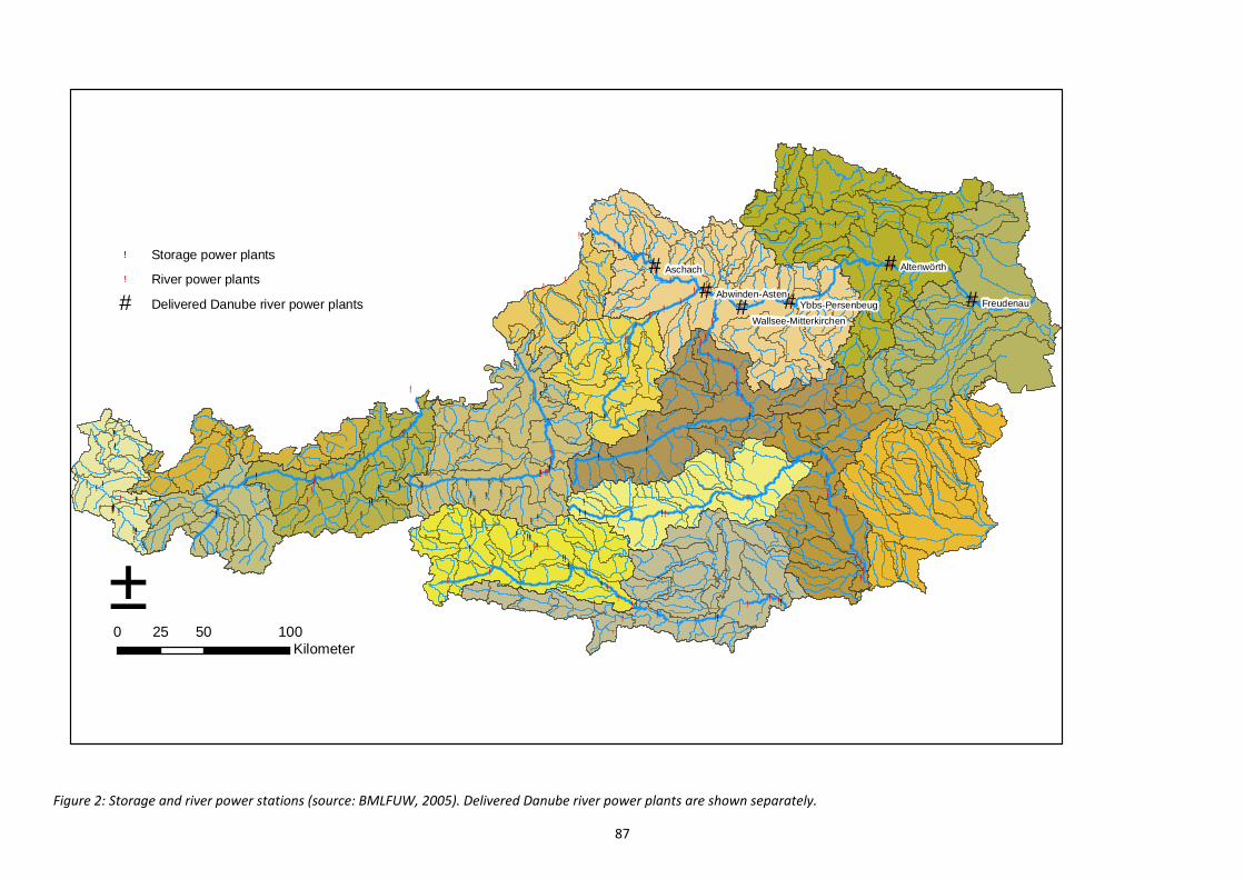
87

Figure 2: Storage and river power stations (source: BMLFUW, 2005). Delivered Danube river power plants are shown separately.

#

###

#

#

!!

!!

!

!

!

!

!

!

!

!!!!

! !

!!

!!!

!

!

!

!

!!

!!!

!

!!

!

!

!

!!

!!

!!

!

! !

!!

!! !

! !!!!!!!

!

!!!!!

! !!!!

!!

!

!!!

! !!

!

! !! ! !!

!! !!

!!!!

!!

!

!!

!!!

!!

!!

!!

!!

!

!!

!!

!

!

!

!

!!

!!!!

!!

!!!!

!!!

!

!!

!

!

!

!!!

!!!!!!

!!!

!!!

!

!

!!

!

!

!

!

!

!

!

!

!!

Aschach

Freudenau

Altenwörth

Abwinden-AstenYbbs-Persenbeug

Wallsee-Mitterkirchen

0 50 10025Kilometer

±

! Storage power plants

! River power plants

# Delivered Danube river power plants

88

9.2. Estimation of the Swiss and German Inn and the German Danube

The water balance model only covers Austrian catchments. Therefore, seperate calculations had to

be performed to estimate the inflow of the Inn river from Switzerland, the runoff contributions of the

German areas to the Inn and the Danube from Germany.

Observations of runoff for the gauging station Martina at the border between Switzerland and

Austria were provided by the Swiss Federal Office for the Environment (Bundesamt für Umwelt

BAFU). Mean monthly correlation‐values between these obervations and simulations of subbasin

0309 of the Inn basin (Figure 1) were determined. These values were also used for the estimation of

inflow from Switzerland in the future scenarios.

For the estimation of the German Inn, the runoff values of the low lying catchments of the Austrian

Inn (subbasin 0601, 0602, 0603, 0604, 0605, 0606, 0411, 0511 ‐ Figure 1) were extrapolated, taking

into account the ratio between the areas of the Austrian and German Inn. The overall Inn was then

calculated as the sum of the German contribution and the runoff contributions of the Austrian

catchments, including the Swiss share. This method is also applied for the future scenarios.

Similar to the estimation of the Swiss Inn, mean monthly correlation‐values were determined

between the overall Inn and German Danube based on values provided by Kling et al. (2012a –

RegCM and Aladin; 2012b – REMO‐UBA) for the reference period 1961 ‐ 1990. These values were

used to calculate runoff in the German Danube in the future, with the overall Inn as a basis. Changes

in seasonality – which show different characteristics for the German Danube than for the more alpine

Inn – are considered by incorporating the future runoff simulations of Kling et al. (2012a, 2012b).

Kling et al. (2012a, 2012b) use the same climate models as applied in PRESENCE, but the period of

2051‐2080 is not analysed in their study. From their results for 2021‐2050 and 2071‐2100, mean

monthly runoff for 2051‐2080 was derived by linear interpolation. These results were then used to

correct the seasonal course of runoff in the German Danube. This is regarded as reasonable, as

seasonal changes are triggered strongly by temperature change, which shows a constant rate of

increase in the climate models. The mean runoff is not corrected, but used from the water balance

model simulations for the Inn (Figure 3), which incorporate the actual long term fluctuation of

precipitation in the climate model data for the period of 2051‐2080.

Figure 3: Mean monthly runoff conditions of the German Danube (RegCM3 2051 – 2080) with and without consideration of a seasonal shift.

0

250

500

750

1000

1 2 3 4 5 6 7 8 9 10 11 12

m³/s

Month

Danube Kling 2065 Danube from Inn (2051‐2080) ‐ without seasonal shift

Danube from Inn (2051‐2080) ‐ including seasonal shift

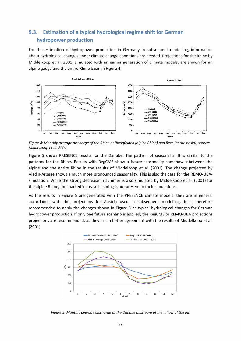
89

9.3. Estimation of a typical hydrological regime shift for German

hydropower production

For the estimation of hydropower production in Germany in subsequent modelling, information

about hydrological changes under climate change conditions are needed. Projections for the Rhine by

Middelkoop et al. 2001, simulated with an earlier generation of climate models, are shown for an

alpine gauge and the entire Rhine basin in Figure 4.

Figure 4: Monthly average discharge of the Rhine at Rheinfelden (alpine Rhine) and Rees (entire basin); source: Middelkoop et al. 2001

Figure 5 shows PRESENCE results for the Danube. The pattern of seasonal shift is similar to the

patterns for the Rhine. Results with RegCM3 show a future seasonality somehow inbetween the

alpine and the entire Rhine in the results of Middelkoop et al. (2001). The change projected by

Aladin‐Arpege shows a much more pronounced seasonality. This is also the case for the REMO‐UBA‐

simulation. While the strong decrease in summer is also simulated by Middelkoop et al. (2001) for

the alpine Rhine, the marked increase in spring is not present in their simulations.

As the results in Figure 5 are generated with the PRESENCE climate models, they are in general

accordance with the projections for Austria used in subsequent modelling. It is therefore

recommended to apply the changes shown in Figure 5 as typical hydrological changes for German

hydropower production. If only one future scenario is applied, the RegCM3 or REMO‐UBA projections

projections are recommended, as they are in better agreement with the results of Middelkoop et al.

(2001).

Figure 5: Monthly average discharge of the Danube upstream of the inflow of the Inn

0

250

500

750

1000

1250

1500

1 2 3 4 5 6 7 8 9 10 11 12

m³/s

Month

German Danube 1961‐1990 RegCM3 2051‐2080

Aladin‐Arpege 2051‐2080 REMO‐UBA 2051 ‐ 2080

austrian climate research program - tu wien · acrp ‐ austrian climate research program ......

Documents