auroral plasma dynamics revealed through radio … hirsch, hassan akbari, chhavi goenka, matt...
TRANSCRIPT

Auroral Plasma Dynamics Revealed through Radio-Optical Sensor FusionJoshua SemeterBoston University Center for Space Physics
Acknowledgements: Sebastijan Mrak, Brent Parham, Nithin Sivadas, John Swoboda, Michael Hirsch, Hassan Akbari, Chhavi Goenka, Matt Zettergren, Marcos Diaz

Solar wind - Magnetosphere Coupling: Energy Storage and Release
Magnetopause!BIMF!
Bow
Sho
ck!
Solar Wind!
Inductive energy is accumulated in the magnetotail via interaction with the solar wind. Stored energy is released impulsively into the atmosphere as heat, ionization, radiation, and bulk acceleration of gases.

Geospace multiscale mission
Spherical harmonic expansion
1 µA/m2
North

Incoherent Scatter Radar
4
SondrestromPoker Flat
Millstone Hill
ESR
EISCAT
Arecibo
Resolute Bay
Jicamarca
ESR
EISCAT
Sondrestrom
Millstone Hill
Arecibo
Jicamarca
PFISR
RISR

27
Figure 2·4: Longitudinal modes of a plasma. Blue lines relate to ionacoustic waves and red ones to Langmuir waves.
plasma particles start to interact more strongly with the growing wave, e.g., by heating.
This can sometimes be described in terms of the so-called quasi-linear saturation within
the Vlasov theory.
A way of categorizing plasma instabilities is to divide them between macroscopic (con-
figurational) and microscopic (kinetic) instabilities. The division is the same as within
plasma theory in general. A macroinstability is something that can be described by
macroscopic equations in the configuration space. Examples of a macroinstability are the
Rayleigh-Taylor, Farley-Buneman and Kelvin-Helmholtz instabilities. On the other hand,
a microinstability takes place in the (x,v)-space and depends on the actual shape of the
distribution function. A consequence of a microinstability is a greatly enhanced level of
fluctuations in the plasma associated with the unstable mode. These fluctuations are called
microturbulence. Microturbulence can lead to enhanced radiation from the plasma and to
enhanced scattering of particles, resulting in anomalous transport coe⇤cients, e.g., anoma-
lous electric and thermal conductivities. Examples of microinstability are the beam-driven,
ion acoustic and electrostatic ion cyclotron instabilities.
31
Figure 2·5: The top figure shows an Incoherent Scattering Spectrum,including the three lines. The middle figure shows a zoom to the ion acousticline, which is the focus of this research. The bottom figure shows theautocorrelation function �(⇥) of the ion acoustic line. f+ is the Dopplerfrequency associated with the ion acoustic phase velocity.
Ti/mi
Te/Ti
Vi
area ~ Ne
Ion-acoustic
DIAZ ET AL.: BEAM-PLASMA INSTABILITY EFFECTS ON IS SPECTRA X - 5
can account for the simultaneous enhancement in the two ion lines, and the simultaneous55
ion and plasma line enhancement.56
This purpose of this paper is to provide a unified theoretical model of modes expected in57
the ISR spectrum in the presence of field-aligned electron beams. The work is motivated58
by the phenomenological studies summarized above, in addition to recent theoretical59
results–in particular, those of Yoon et al. [2003], and references therein, which suggest60
that Langmuir harmonics should arise as a natural consequence of the same conditions61
producing NEIALs. Although these e�ects have been treated in considerable detail in the62
plasma physics literature, their implications for the field of ionospheric radio science (and63
ISR in particular) have not yet been discussed. The conditions to detect all the modes64
present within the IS spectrum within the same ISR is also presented in this work.65
2. Plasma in Thermal Equilibrium
There exist two natural electrostatic longitudinal modes in a plasma in thermal equilib-66
rium: the ion acoustic mode, which is the main mode detected by ISRs, and the Langmuir67
mode [Boyd and Sanderson, 2003]. Using a linear approach to solve the Vlasov-Poisson68
system of equations, the dispersion relation of these modes is obtained. The real part of69
the ion acoustic dispersion relation reads70
⇥s = Csk, (1)
and the imaginary part (assuming ⇥si � ⇥s, k2�2De � 1 and Ti/Te � 1) can be written71
as72
D R A F T May 29, 2010, 6:36am D R A F T
X - 6 DIAZ ET AL.: BEAM-PLASMA INSTABILITY EFFECTS ON IS SPECTRA
⇤si = �
⇥
8
⇧�me
mi
⇥ 12
+
�Te
Ti
⇥ 32
exp
⇤� Te
2Ti� 3
2
⌅⌃⇤s (2)
where Cs =⌥
kB(Te + 3Ti)/mi is the ion-acoustic speed. The dependence of this mode
on ionospheric state parameters is observed in Eq. 2. The Langmuir mode is detected by
ISR under certain conditions, and the real part of its dispersion relation is expressed as
⇤L =�
⇤2pe + 3 k2 v2
the ⇥ ⇤pe +3
2vthe�Dek
2, (3)
and the imaginary part (assuming ⇤Li ⇤ ⇤L) is73
⇤Li ⇥ �
⇥
8
⇤3pe
k3
1
v3the
exp
⇤�
⇤2pe
2k2v2the
� 3
2
⌅⇤L. (4)
The forward model used to estimate ionospheric parameters in ISR assumes that these74
are the dominating modes in the ISR spectrum. However, an injected beam of particles,75
in particular electrons, can destabilize the plasma, altering the dispersion relations and76
amplitudes of these modes.77
3. Current Model of the Langmuir Decay Process for NEIAL Formation
The model presented by Forme et al. [1993] to explain NEIALs is a two step process.
First, a beam-plasma instability enhances Langmuir Waves (LW). Second, if the enhance-
ment of LW is high enough then the enhanced LW can decay, enhancing Ion Acoustic
Waves (IAWs) and counter-propagating LWs. The plasma-beam process involves three
species: thermal electrons, thermal ions, and an electron beam with a bulk velocity of
vb. By assuming small perturbations and small damping/growth (vthe, vthi, vb ⇤ ⇤/k),
linearization of Vlasov-poison system can be used to find the dispersion relation of the
D R A F T May 29, 2010, 6:36am D R A F T
Langmuir
X - 6 DIAZ ET AL.: BEAM-PLASMA INSTABILITY EFFECTS ON IS SPECTRA
⇤si = �
⇥
8
⇧�me
mi
⇥ 12
+
�Te
Ti
⇥ 32
exp
⇤� Te
2Ti� 3
2
⌅⌃⇤s (2)
where Cs =⌥
kB(Te + 3Ti)/mi is the ion-acoustic speed. The dependence of this mode
on ionospheric state parameters is observed in Eq. 2. The Langmuir mode is detected by
ISR under certain conditions, and the real part of its dispersion relation is expressed as
⇤L =�
⇤2pe + 3 k2 v2
the ⇥ ⇤pe +3
2vthe�Dek
2, (3)
and the imaginary part (assuming ⇤Li ⇤ ⇤L) is73
⇤Li ⇥ �
⇥
8
⇤3pe
k3
1
v3the
exp
⇤�
⇤2pe
2k2v2the
� 3
2
⌅⇤L. (4)
The forward model used to estimate ionospheric parameters in ISR assumes that these74
are the dominating modes in the ISR spectrum. However, an injected beam of particles,75
in particular electrons, can destabilize the plasma, altering the dispersion relations and76
amplitudes of these modes.77
3. Current Model of the Langmuir Decay Process for NEIAL Formation
The model presented by Forme et al. [1993] to explain NEIALs is a two step process.
First, a beam-plasma instability enhances Langmuir Waves (LW). Second, if the enhance-
ment of LW is high enough then the enhanced LW can decay, enhancing Ion Acoustic
Waves (IAWs) and counter-propagating LWs. The plasma-beam process involves three
species: thermal electrons, thermal ions, and an electron beam with a bulk velocity of
vb. By assuming small perturbations and small damping/growth (vthe, vthi, vb ⇤ ⇤/k),
linearization of Vlasov-poison system can be used to find the dispersion relation of the
D R A F T May 29, 2010, 6:36am D R A F T
700
400
100
Alti
tude
(km
)
-10 +10 Frequency (kHz)
Ne
=!2pe
✏o
me
e2(1)
!pe
=
sN
e
e2
✏0me
(2)
1
Ne
=!2pe
✏o
me
e2(1)
!pe
=
sN
e
e2
✏0me
(2)
!s
(3)
1
Ne
=!2pe
✏o
me
e2(1)
!pe
=
sN
e
e2
✏0me
(2)
�!s
(3)
1
Incoherent Scatter Radar
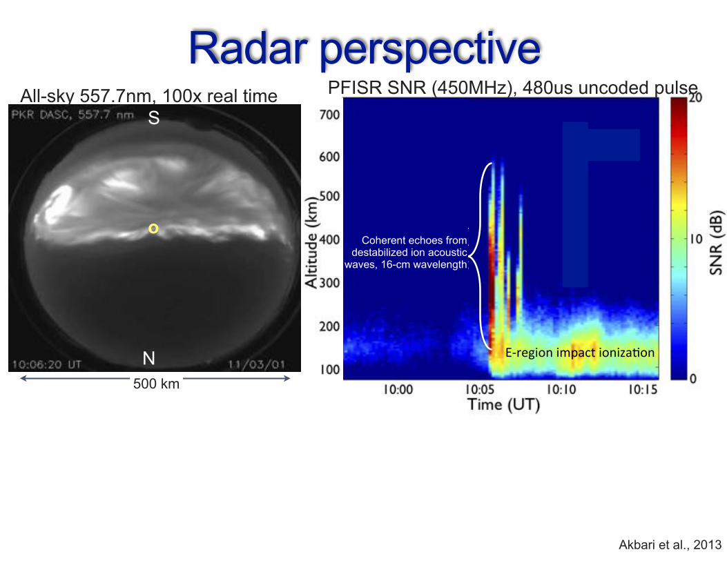
Radar perspectiveS
N
o
All-sky 557.7nm, 100x real time PFISR SNR (450MHz), 480us uncoded pulse
500 km
E"region)impact)ioniza0on)
satellite)
Coherent)UHF)sca8er)caused)by)Langmuir)
turbulence)at)leading)edge)of)storm)
expansion.))
Coherent echoes fromdestabilized ion acoustic
waves, 16-cm wavelength
Akbari et al., 2013

Frequency (kHz)-10 +10
700
500
300
100
Alti
tude
(km
)
700
500
300
100
Alti
tude
(km
)Radar perspective
PFISR SNR (450MHz), 480µs uncoded pulse
E"region)impact)ioniza0on)
satellite)
Coherent)UHF)sca8er)caused)by)Langmuir)
turbulence)at)leading)edge)of)storm)
expansion.))
Coherent echoes fromdestabilized ion acoustic
waves, 16-cm wavelength
10:05:43
10:05:32
700
500
300
100
Alti
tude
(km
)10:05:26
Candidate mechanisms: 1. Parametric decay of Langmuir turbulence (beam related) 2. ion-electron streaming instability (current related)
Akbari et al., 2013

Optical manifestation of dispersive bursts
to account for the observed discrepancy through suchadditional sources. If one considers only the electron impactsource for both emissions, the resulting OII(732–733 nm)and OI(630 nm) emission profiles will be nearly propor-tional since O+(2P) and O(1D) are both excited from theisotropic secondary electron population. Current modelspredict that all additional sources of auroral OI(630 nm)peak at higher altitudes than the electron impact source,hence raising the OI(630 nm) emission peak with respect tothe OII(732–733 nm) peak. The mechanism we requiremust have exactly the opposite effect.[18] The cause of the observed altitude separation thus
remains unclear. The extreme altitude separation is sugges-tive of an additional source for auroral O+(2P), perhaps viadirect excitation of ambient O+(4S ) atoms. Another contri-buting factor could be a significant underestimation of thecurrently accepted rate coefficients for O+(2P) quenchingvia O and N2. Increased quenching would decrease prefer-entially lower altitude O+(2P) thus raising the expectedemission peak. The model results reported by Semeter etal. [2001], for example, used the quenching rates of Ruschet al. [1977], which were found by Bucsela et al. [1998] toprovide a better fit to their 247 nm measurements than thehigher Chang et al. [1993] results. Still another contributingmechanism could be vertical transport of O+. Such ion up-flows are commonly observed by IS radars at aurorallatitudes [Ogawa et al., 2000] and by polar orbiting satel-lites at the polar cap boundary [McFadden et al., 2001].
Because of the 5 s radiative lifetime of the forbiddenOII(732–733 nm) emission, vertical transport would causethe emission to be ‘‘smeared’’ upward along the field line.The distinct separation of the OII(732–733 nm) and OI(630nm) emission peaks seen in Figure 2, however, could not beproduced by this mechanism.
6. Summary
[19] The contribution of this work is twofold. First, wehave described a technique for isolating the OII(732–733nm) doublet in auroral imagery by means of its altitudeseparation from the competing N2(1PG) source in the 732–773 nm band. Second, we have used this technique todiscover a significant altitude separation between theOII(732–733 nm) and OI(630 nm) emission peaks in aseries of tall auroral rays observed near the polar capboundary. The >100 km offset between the emission peaksis inconsistent with published predictions; further modelingis required to understand this result.
[20] Acknowledgments. The author thanks Jeffrey Thayer, DirkLummerzheim, and Richard Doe for valuable discussions, and the Son-drestrom site crew for support during the November 2001 campaign. Thiswork was partially supported by NSF grant ATM-9813556.
ReferencesBucsela, E., et al., Atomic and molecular emissions in the middle ultravioletdayglow, J. Geophys. Res., 103, 29,215–29,228, 1998.
Chamberlain, J., Physics of the Aurora and Airglow, Academic, New York,1961.
Chang, T., et al., Reevaluation of the O+(2P) reaction rate coefficientsderived from Atmosphere Explorer C observations, J. Geophys. Res.,98, 15,589–15,597, 1993.
Lummerzheim, D., et al., The application of spectroscopic studies of theaurora thermospheric neutral composition, Planet. Space Sci., 38, 67–78,1990.
McFadden, J., et al., FAST observations of ion outflow associated withmagnetic storms, Space Weather, Geophysical Monograph, 125, 413,2001.
Meier, R., et al., Deducing composition and incident electron spectra fromground-based auroral optical measurements: A study of auroral red lineprocesses, J. Geophys. Res., 94, 13,541–13,552, 1989.
Ogawa, Y., et al., Simultaneous EISCAT Svalbard and VHF radar observa-tions of ion upflow at different aspect angles, GRL, 27, 81–84, 2000.
Omholt, A., The red and near-infrared auroral spectrum, J. Atmos. Terr.Phys., 10, 320–331, 1957.
Rees, M., et al., The production efficiency of O+(2P) ions by auroral elec-tron impact ionization, J. Geophys. Res., 87, 3612–3616, 1982.
Rees, M. H., and R. Jones, Time-dependent studies of the aurora-II. Spec-troscopic morphology, Planet. Space Sci, 21, 1213–1235, 1973.
Rusch, D., et al., The OII(7319–7330 A) dayglow, J. Geophys. Res., 82,719–722, 1977.
Semeter, J., et al., Simultaneous multispectral imaging of the discrete aur-ora, J. Atmos. Sol. Terr. Phys., 63, 1981–1992, 2001.
Sivjee, G., et al., Intensity ratio and center wavelengths of OII (7320–7330 A) line emissions, The Astrophysical Journal, 229, 432–438, 1979.
Sivjee, G., et al., Variations, with peak emission altitude, in auroral O2
atmospheric (1,1)/(0,1) ratios and its relation to other auroral emissions,J. Geophys. Res., 104, 28,003–28,018, 1999.
Solomon, S., et al., The auroral 6300 A emission: Observations and mod-eling, J. Geophys. Res., 93, 9867–9882, 1988.
Strickland, D., et al., Deducing composition and incident electron spectrafrom ground-based auroral optical measurements: Theory and results,J. Geophys. Res., 94, 13,527–13,539, 1989.
Torr, M., and D. Torr, The role of metastable species in the thermosphere,Rev. Geophys., 20, 91–144, 1982.
!!!!!!!!!!!!!!!!!!!!!!!J. Semeter, SRI International, 333 Ravenswood Avenue, Menlo Park, CA
94025, USA. ([email protected])
Figure 2. (a) Brightness versus elevation angle along theflux tube indicated by the arrows in Figure 1, lower right.(b) Geometry used to extract altitude emission profiles. (c)Brightness versus altitude, resolved using the geometricmodel of Figure 2b. (d) The pure OII (732–733 nm) profileafter subtraction of N2 (1PG) contribution, compared withOI (630 nm).
29 - 4 SEMETER: COMPARISON OF EMISSIONS IN AURORAL RAYS
50 fps
A
3 keV
0.5 keV
X - 30 DAHLGREN ET AL.: DISPERSIVE FIELD-ALIGNED AURORAL BURSTS
10:06:12.040 UT
A
B
10:06:15.200 UT
C
D
Figure 4. CMOS images with the four flaming rays marked. Most of the rays ex-
perienced flaming motion at the time of observations and these events were chosen for
detailed study.
11.85 11.9 11.95 12 12.05 12.1 12.15 12.2 12.25 12.3 12.35110
120
130
140
150
160
170
flaming vel: 80 km/s
11.85 11.9 11.95 12 12.05 12.1 12.15 12.2 12.25 12.3110
120
130
140
150
160
170
11.9 12 12.1 12.2 12.3 12.4 12.5110
120
130
140
150
160
170
11.9 12 12.1 12.2 12.3 12.4 12.5110
120
130
140
150
160
170A BRadial keogram for event A
Seconds after 10:06:00 UT
Seconds after 10:06:00 UT
Alt
itu
de
(km
)A
ltit
ud
e (
km)
Emission profiles for event A
Radial keogram for event B
Emission profiles for event B
Seconds after 10:06:00 UT
Seconds after 10:06:00 UT
Alt
itu
de
(km
)A
ltit
ud
e (
km)
Figure 5. Top panels: Radial keograms for events A and B. The radial distance from
the center of the image is translated to altitude, assuming the emission peak is at 120 km
at the start of the flaming. The bottom panels show the brightness as line plots for each
time, as a function of altitude. The maximum brightness of each profile is marked with
a red star, and a linear fit gives flaming velocities of 80 ± 12 km/s for event A and
93 ± 19 km/s for event B.
D R A F T June 14, 2013, 11:36am D R A F T
Seconds after 10:06:00 UT
Dahlgren et al., JGRA 2013
X - 32 DAHLGREN ET AL.: DISPERSIVE FIELD-ALIGNED AURORAL BURSTS
12 12.5 13 13.5 14 14.5 151.4
1.6
1.8
2
2.2
2.4x 10⁴ Zenith brightness
Time after 10:06 UT (s)
Brig
htne
ss
0 1 2 3 4 5 6 7 8 9 100
0.5
1
1.5
2x 10⁷ Power spectral density
Frequency (Hz)
Pow
er
Figure 7. Top panel: Integrated brightness in a region of 10 × 10 pixels around
magnetic zenith. Bottom panel: The power spectral density estimate shows quasiperiodic
oscillations at 2.4 Hz.
D R A F T June 14, 2013, 11:36am D R A F T
2.4 Hz
Power spectral density
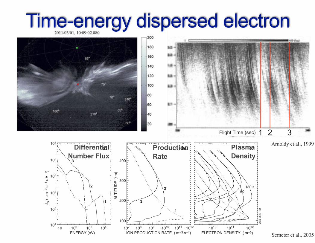
Average energy of primary electrons decreases from 3keV to <500eV in 0.2-s.
Field-aligned bursts are periodic at ~2.4Hz
ARNOLDY ET AL.: ENERGY AND PITCH ANGLE AURORAL ELECTRONS 22,615
Finally, at energies of the inverted-V peak and extending down to very low energies (tens of eV) there is a third com- ponent which is very field-aligned. The degree of field- alignment (evident in subsequent figures) gives a measure of the perpendicular characteristic energy of the electrons. The PHAZE data give a characteristic energy of ---t0 eV for this component, however, with higher-resolution pitch angle data, McFadden et al. [1986] have measured a characteristic energy of a few eV. Of interest in this paper is the relationship be- tween the hot inverted-V electrons and the cold FABs. Figure t shows that in the absence of the FABs (590 s for example) the inverted-V electrons are quite "monoenergetic," while dur- ing FABs they are severely modified as will now be discussed.
2.1. The 476-484 s Flight Time Between these flight times, as can be seen in Figure 1, the
FABs were present, abruptly turned off, and then returned. This is best presented via the pitch angle spectrograms in Plate t. Each horizontal panel is a pitch angle versus time spectro- gram at a fixed energy (t0 _+ 0.5 keV top panel to 50 _+ 0.25 eV bottom panel) with the count rate given by the color. These pitch angle spectrograms were made with fixed-energy, top-hat detectors sampling 15 pitch angle bins 18 ø wide in pitch angle each at a rate of 125 samples/s. The five pitch angle bins centered ---0 ø had a resolution of 5 ø and were sampled at a rate of 2 kHz.
The FABs, extending over a wide range of energy, from 10 keV to several tens of eV, are evident in Plate 1 as high count rates, or the only count rate, near 0 ø pitch angle. As discussed above, their spread in pitch angle is very small (an order of magnitude drop in count rate over t0 ø of pitch angle) indicat- ing that they were accelerated along B from a very cold pop- ulation. The FABs ceased at ---479 s, and returned again at 482 s. During this time interval the inverted-V electrons, de- tected only by the t0 and 5 keV detectors, were fairly isotropic in pitch angle up to the loss cone and showed little time variability in pitch angle. However, during the FABs the elec- trons measured at t0 keV are very sporadic and clearly show dispersed structure with the larger pitch angles detected at later times. The characteristic energy of these electrons are typical for inverted-V electrons, a few keV.
At earlier and later times (such as 476 and 484 s) the dis- persed structures in the inverted-V electrons are not evident but rather there appears to be an enhanced continuum of particles. During these times one can use the 0 ø pitch angle electrons, sampled at 2 kHz, to look for structure. Plate 2 consists of two plots, one during the time of no field-aligned electrons (480-481 s) and the other during a period of FABs (484-485 s). The top panel of these plots gives the raw count rate of t0 keV, 0 ø pitch angle, electrons while the bottom panel is a frequency versus time spectrogram. There is no evidence of periodic structures in the inverted-V electrons in the 480-481 s plot during a period of no FABs. The data taken during the FABs show significant power at ---80 Hz. Whether this is just the repetition rate of cold, t0 keV FAB electrons and not the hot inverted-V, 0 ø pitch angle electrons cannot be determined. It is suggestive, however, that the continuum count rate at larger pitch angles is due to pitch angle-dispersed structures that are fluctuating at 80 Hz.
As can be seen in Figure t, there were many instances of FABs during the PHAZE II flight as indicated by the streaks of electrons of energy below the inverted-V potential. To see the pitch angle-dispersed signature, such as evident in Plate 1,
Electrons (counts/see)
I t ..................... • .... .•-•-• • .............................. - -•-----'• .......... ,•" .... .......... 400
30'0 I '" '?:' '.'- .................. ..... ,: . • t .• '"5"• ,•---':-'-- ' '"•q:•:;;'•;;•. :•:•'.* ........ <•----:•. •,• .;•25•,•? -'•:' •.•::• '? -•' '• ............. '•-, ...... ':• .... *:-. ' 8.0 ' ....... .,•'.:I;.,. ""-½•?;-7•..-C::">'L•;[: .•:•.:.--:V';" '; *. 7 ...... .' :-' '-.' "::•::"')::.•/',.•;•'•:•}?v"-"---':•..'•&•'"•'•,:• ..::•..:..'.-•:•-,-.-'::: ....
"':' ..... • •.";•..:-'.:.'•" • •'4 ' ;'.*-. 6.0
.
..
4.0 ...
./
3.0 . ß
/....,.
2.0 •&;.:->.• •.,.•,•.: .•.-•.• .... • ..•; •. ..?!•.•..,,....,..•:•.i'•......•-..-: ' 3.30 335
.... t ........... ' .... '7""'.'. i '. i ..... 40o
;" > ";" •"i'•' •' '-- •:•'"•:'•:'""
•!• .• • [•i',,•.'-'..-.':..'.: "........•,:..--•.'::•:•-"•"-'•"" ""•.•• •. .••••,;.: !•:. :;•;•v•.',•:•--::•e-"•,•-::..• - -•;:::'•: .::il •',' I• •' <'•,.,';•:•:'.. :.•':::'-"'•" '*' "½" •"" ' •' ''" ' •..'' '•" ""'••'-- - '•••;:.4-
"."-..• ..... ":.':'•..• • ...... • •'. :'• -".-.-•: .'-};v'-• • *-.:.':• •. •". ....... .: s :•i•"':.'- •-'•J '!•.::•.,. '-. ;: '•::.. '";'-.:--....-...¾•' •'•:."•- .•":. ,,-[?
..... : 'ii!il ...... O.l
0.03
Flight Time (see)
Figure 2. Energy versus time spcctrograms from two differ- ent electron detectors. •hc gray scale gives the detector count rate in units of 10 3 counts/s.
there had to be one of the fixed energy, top-hat detectors at the energy of the inverted-V potential, and the repetition rate of the bursts had to be resolvable by the detector whose Nyquist frequency was 62.5 Hz. If the later condition was not satisfied, then it was almost always the case that a frequency analysis of the rapidly sampled 0 ø pitch angle pad of the detector, such as discussed above, would reveal fluctuations in count rate be- tween 80 and tOO Hz. One should notice in Plate 1 that only the fixed-energy detector at or near the inverted-V potential has the dispersed structure. Lower energies measured for the same event are considerably reduced in intensity and have no clear organization into dispersed signatures. McFadden et al. [1988] report similar observations where electrons at or above the spectral peak energy (inverted-V energy) displayed coher- ent flux oscillations between 50 and 125 Hz. These oscillations
were not seen at energies below the spectral peak. FABs fluc- tuated between 4 and t0 Hz, sometimes alone, and at other times coincident with the higher frequency fluctuations of the high-energy electrons. The difference between the McFadden et al. [1988] results and the ones presented here is that the PHAZE data gives the pitch angle dispersion of the fluctuating inverted-V electrons in addition to the energy (velocity) dis- persion of the FABs.
2.2. The 330-340 s Flight Time This is a period of intense FABs and when flickering aurora
could easily be identified in the ground all-sky camera data. Figure 2 gives two energy versus time spectrograms from two
Production Rate
Plasma Density
1 2 3
Differential Number Flux
Arnoldy et al., 1999
Semeter et al., 2005
keV
Flight Time (sec)
180 s
3
3
2 2
1
1
60
103
v04-
030-
10
100
200ALTI
TUDE
(km
)
300
400
10 102 103 104 108107 1010 10111011109 1012 10121010
ENERGY (eV) ION PRODUCTION RATE ( m–3 s–1) ELECTRON DENSITY ( m–3)
ENERGY DEPOSITION RATE (eV cm–3 s–1)107103 105104 106
a. b. c.
104
105
106
107
108
109
J N (
cm–2
s–1
eV
–1)
Time-energy dispersed electron

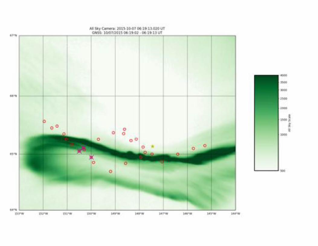
Mahali Experiment
146150 142Latitude
64
66
67
65Long
itude
Pankratius et al., IEEE Comm. Mag., 2016, Semeter et al., GRL 2017, Mrak et al JGRA 2017
https://mahali.mit.edu


145150 145150 145150 14515064
66
64
66
64
66
West Geographic Longitude
Geo
grap
hic
Latit
ude
a) 06:18:24-35 b) 06:18:37-48 c) 06:18:49-00 d) 06:19:02-13
e) 06:19:14-25 f) 06:19:27-38 g) 06:19:39-50 h) 06:19:52-03
i) 06:20:04-15 j) 06:20:17-28 k) 06:20:29-40 l) 06:20:42-53
Strong phase scintillation observed only along the trailing edge of the westward traveling surge
Semeter et al., GRL 2017, Mrak et al JGRA 2017

Conclusion• Dissipation of magnetospheric free energy occurs through a cascade
of spatial scales, extending from ~100 km to ~10 cm.
• The role of small scale variability in modifying the energy dissipation process is poorly understood.