arX

iv:1

608.

0260

6v2

[he

p-th

] 2

2 Fe

b 20

17

Three-dimensional noncommutative Yukawa theory:

Induced effective action and propagating modes

R. Bufalo1∗and M. Ghasemkhani2†1Departamento de Fısica, Universidade Federal de Lavras,

Caixa Postal 3037, 37200-000 Lavras, MG, Brazil

2Department of Physics, Shahid Beheshti University,

G.C., Evin, Tehran 19839, Iran

February 23, 2017

Abstract

In this paper we establish the analysis of noncommutative Yukawa theory, encom-passing neutral and charged scalar fields. We approach the analysis by consideringcarefully the derivation of the respective effective actions. Hence, based on the obtainedresults, we compute the one-loop contributions to the neutral and charged scalar fieldself-energy, as well as to the Chern-Simons polarization tensor. In order to properlydefine the behaviour of the quantum fields, the known UV/IR mixing due to radiativecorrections is analysed in the one-loop physical dispersion relation of the scalar andgauge fields.

PACS: 11.15.-q, 11.10.Kk, 11.10.Nx

∗E-mail: rodrigo.bufalo@dfi.ufla.br†E-mail: ghasemkhani@ipm.ir

1

Contents

1 Introduction 3

2 General discussion 5

3 Perturbative effective action 7

3.1 Neutral scalar fields . . . . . . . . . . . . . . . . . . . . . . . . . . . . . . . . 7

3.1.1 φφ contribution . . . . . . . . . . . . . . . . . . . . . . . . . . . . . . 8

3.1.2 φφφ contribution . . . . . . . . . . . . . . . . . . . . . . . . . . . . . 9

3.2 Charged scalar fields . . . . . . . . . . . . . . . . . . . . . . . . . . . . . . . 10

3.2.1 φφA contribution . . . . . . . . . . . . . . . . . . . . . . . . . . . . . 11

3.2.2 φφAA contribution . . . . . . . . . . . . . . . . . . . . . . . . . . . . 12

4 Propagating modes scalar field 13

5 Propagating modes charged scalar fields 14

5.1 Dispersion relation charged scalar fields . . . . . . . . . . . . . . . . . . . . . 15

5.2 Dispersion relation gauge field . . . . . . . . . . . . . . . . . . . . . . . . . . 17

6 Concluding remarks 20

A Non-planar integrals 21

B Effective action 22

B.1 φφA contribution . . . . . . . . . . . . . . . . . . . . . . . . . . . . . . . . . 22

B.2 φφAA contribution . . . . . . . . . . . . . . . . . . . . . . . . . . . . . . . . 23

C Dispersion relation 24

2

1 Introduction

The field theoretical model for description of the interaction between nucleons in particlephysics was first proposed by H. Yukawa in 1935 [1], which led to the prediction of pionbefore its discovery from cosmic rays in 1947 [2]. The Yukawa term originates from theexchange of a massive scalar field that in the non-relativistic limit yields a Yukawa potentialand hence the corresponding force has a finite range, which is inversely proportional to themediator particle mass.

Since its proposal, the notion of Yukawa potential has been used in different areas inthe description of several phenomena such as chemical process, astrophysics, fluid plasmasystem and especially in modern particle physics. More importantly, in the latter case, i.e.standard model, the Yukawa interaction of the Higgs field and massless quarks and leptonsis the responsible coupling to give mass to these fermionic fields.

Due to its importance in the different physical phenomena, Yukawa theory has been usedas a laboratory in the search of physics beyond standard model, or even to scrutinize thecornerstones of gauge theories. Furthermore, if we expand our scope and add to our inter-est the description of nature behavior at shortest distances [3, 4], i.e. a quantum theory ofgravity, or even the so-called minimal length scale physics, one inexorably finds that noncom-mutative geometry is one of the most highly motivated and richer framework [5], includingphenomenological inspirations [3, 6–9]. Space-time noncommutativity naturally emerges atPlank scale in attempts to accommodate quantum mechanics and general relativity in a com-mon framework, one finds uncertainty principles that are compatible with non-commutingcoordinates [10, 11].

The simplest realization of noncommutativity is given by the following canonical algebra

[xµ, xν ] = iθµν . (1.1)

where θµν is a constant skewsymmetric matrix of dimension of length squared. These com-mutation relations give an uncertainty relation among the coordinates: ∆xµ ∆xν & 1

2|θµν |.

Notice, however, that the nonzero components of θµν are arbitrary parameters that mustbe constrained by experiments, we can think as they being the resolution scale that can betaken to be, for instance, of the order of square of Planck length ℓP l.

A suitable framework to compute quantities in a NC–QFT is by the use of Weyl-Moyal(symbol) correspondence [12]. This allows to define a classical (commutative) analogue ofthe noncommutative space, so that the following relation holds: ϕ (x)ψ (x) → ϕW ⋆ ψW ,where ϕW is the so-called Weyl symbol of the operator ϕ (x) [12]. Moreover, in this context,we have that the Moyal star product is defined as

f(x) ⋆ g(x) = f(x) exp

(i

2θµν←−∂ µ

−→∂ ν

)g(x). (1.2)

One common property of NC gauge theories that has been uncovered is that high-momentum modes (UV) affect the physics at large distances (IR) leading to the appearanceof the so-called UV/IR mixing [13]. These “anomalies” involve non-analytic behavior inthe noncommutativity parameter θ making the limit θ → 0 singular. Despite of the manyattempts to understand this issue in four and three-dimensional field theory models, see [14]and [15, 16], respectively, no complete description to handle it has yet been provided [17].

3

An important branch of interest regarding NC gauge theories is the study of how non-commutativity affects established properties of conventional theories, in particular a consid-erable effort has been expended in analyzing gauge theories defined in a three-dimensionalnoncommutative spacetime, this effort is highly supported by the fact that wandering intolower-dimensional models has been proved to be very fertile and stimulated significantly thedevelopment of our knowledge in the subject. Gauge theories defined in a three-dimensionalspacetime [18] are known to possess unique properties and are well motivated as providinga simple setting where important theoretical ideas are suitably tested. Noncommutativethree-dimensional field theory, in particular gauge theory, can find application in the studyof planar physics in condensed matter and statistical physics [19–21]. After this observation,various perturbative aspects of the noncommutative Chern-Simons theory have been stud-ied [22–27], NC Maxwell-Chern-Simons theory [28, 29] and NC QED3 [30, 31], as well as itssupersymmetric extension [32], where deviations of known phenomena and interesting newproperties have been uncovered.

However, as we have extensively discussed, in addition to its importance in the StandardModel of particles, a noncommutative extension of the Yukawa field theory action shouldbe fully considered, in particular how the noncommutative Higgs effective action can begenerated. Some aspects for this theory have been discussed previously [33–37].

In particular, our present analysis will be twofold: first, we will consider the interactionbetween a neutral scalar field and dynamical fermionic fields, where the scalar field effectiveaction is found by integrating out the fermionic modes, an additional derivative cubic cou-pling is found for the scalar field. Second, a more interesting case is considered, now we havethe interaction among charged scalar fields with fermionic fields augmented by gauge fields,in which the effective action describing the interaction between the charged scalar and gaugefields is obtained. In the latter, we shall consider the dynamics of the gauge sector given bythe higher-derivative (HD) Chern-Simons action [31], where new features are discussed. Atlast, in both cases, UV/IR mixing is analysed in the one-loop physical dispersion relation ofthe scalar and gauge fields due to radiative corrections, this is justifiable once this anomalymight modify significantly the behavior of the quantum field in the description of a givenphenomen and find room in interesting application [38].

Therefore, in this paper we will consider the effective action for two distinct Yukawacouplings: i) neutral scalar field with fermionic fields, and ii) charged scalar field withfermionic fields plus a gauge field. For this purpose, we will make use of the ideas out-lined in Ref. [31, 39], in which noncommutative fermionic effective actions were considered.The cornerstone of this approach is outlined in Sec. 2 and consists in consider, in a formalway, the existence of an exact Seiberg–Witten map [40], valid to all orders in θ so that thenoncommutative effects into the resulting outcome are in fact nonperturbative. We computeexplicitly in section 3 the respective effective action for the neutral and charged scalar field,where the presence of the new couplings is discussed. Based on the obtained results for theeffective action, we proceed in Sec. 4 to compute the one-loop correction to the self-energy ofthe neutral scalar field, in particular application to its dispersion relation. Next, in Sec. 5, weconsider the effective action obtained for the case of charged scalar fields minimally coupledwith a HD Chern-Simons gauge field, a model that one can name as NC HD-Chern-Simons-Higgs model. In this case we carefully analyse the dispersion relation for both fields, bycomputing the set of diagrams for the respective one-loop self energy functions. Addition-ally to what we have already discussed, another physical application where the present study

4

can be employed, follows from Refs. [41–43] in which it is shown that a model where theChern-Simons term coupled to the scalar field matter is a suitable framework for field the-oretical description of the Aharonov-Bohm effect. At Sec. 6 we summarize our results andpresent our conclusion and prospects.

2 General discussion

Let us now define the noncommutative extension of fermionic fields interacting with a neutralscalar field, which can be named as a noncommutative Yukawa model. For this, we shallconsider the following action

S =

∫d3x

[iψ ⋆ γµ∂µψ −mψ ⋆ ψ + gψ ⋆ φ ⋆ ψ

]. (2.1)

It should be remarked that we are working with a two-component representation for thespinors with the standard convention

γ0 = σ3 =

(1 00 −1

), γ1 = iσ1 =

(0 ii 0

), γ2 = iσ2 =

(0 1−1 0

), (2.2)

where the γ-matrices satisfy γµγν = ηµν − iεµνσγσ. We observe that the action (2.1) isinvariant under a global U(1) symmetry, ψ → eiαψ. Furthermore, on the behavior of thisaction under discrete transformations, parity (P), charge conjugation (C) and time reversal(T), we have prepared a detailed analysis in the following:

(i) Parity

The description of the parity transformation in 2+1 dimensions is given by x1 → −x1and x2 → x2. Using the invariance of the kinetic part of the Dirac Lagrangian underparity, it is found that the fermionic field transforms as ψ → γ1ψ. Hence, it is easilyconcluded that parity is broken by the fermion mass term, since ψψ → −ψψ.From (1.1), it is deduced that the noncommutative parameter changes sign under parityθ → −θ, and hence we observe that the interaction term ψ ⋆ φ ⋆ ψ transforms into thefollowing

SPint

= −g∫d3x ψ ⋆ (ψ ⋆ φ

P), (2.3)

in which we have used the anti-commuting property of the fermionic fields. If weassume a pseudo scalar field φ

P= −φ, similar to the three-dimensional Yukawa term

in commutative space, then it is shown that the Yukawa coupling as considered hereEq. (2.1) is not parity invariant; however, it follows that we can construct a combinationthat is parity invariant

Sint = g

∫d3x ψ ⋆ {φ, ψ}⋆, (2.4)

here { , } = [ , ]+. On the other hand, for the other choice φP= +φ, it is easily

realized that

Sint = g

∫d3x ψ ⋆ [φ, ψ]⋆, (2.5)

is parity invariant.

5

(ii) Charge conjugation

Under a charge conjugation transformation in three dimensions, the spinor field changesas ψ → Cγ0ψ⋆, so that the operator C should satisfy the following relation

C−1γµC = −(γµ)T . (2.6)

Hence, by considering the above constraint and also the representation of the gammamatrices in (2.2), the appropriate choice for the charge conjugation operator in 2 + 1dimensions is given by C = γ2. Since (γ2)⋆ = γ2 and (γ0)⋆ = γ0 then ψ⋆ → γ2γ0ψ, sothat consequently we can find the transformation of the fermion mass term as follows

ψcψc = −ψTγ0ψ⋆ = ψψ, (2.7)

where (γ2)T = −γ2 and the anticommuting property of the spinors had been used. Wethus see that the fermion mass term is C-invariant. Finally, if we consider that thescalar field satisfies φc = φ, the noncommutative Yukawa interaction term transformsas

Scint

= g

∫d3x ψ ⋆ (ψ ⋆ φ) (2.8)

We notice that there are two different choices to build a noncommutative Yukawainteraction term that these are related to each other by a charge conjugation trans-formation. This point was first mentioned in [44], including the study of the discretesymmetries in noncommutative QED4. Furthermore, if we apply θ → −θ to (2.8), wefind that the interaction term is C invariant.

(iii) Time reversal

Time reversal operator acts on the fermionic field as ψ → γ2ψ. Thus the fermionmass term, similar to the parity transformation, is not invariant under T, since itbehaves as ψψ → −ψψ. For the interaction term, we have

STint

= g

∫d3x ψ ⋆ (ψ ⋆ φ) (2.9)

in which it is supposed that φT = −φ. Once again we observe that, similar to thecharge conjugation transformation, adding the assumption θ → −θ gives us a T-invariant interaction term.

Finally, we are able to establish the one-loop effective action for the scalar field φ by inte-grating over the fermionic fields,

iΓ [φ] = lndet (i6∂ −m+ gφ⋆)

det (i6∂ −m)= −

∑

n

1

ntr

(( 6∂ + im)−1 i (gφ⋆)

)n

, (2.10)

where we identify the differential operator as for the fermionic propagator,

( 6∂ + im)−1 δ (x− y) =∫

d3p

(2π)3i ( 6p+m)

p2 −m2 + iεe−ip.(x−y). (2.11)

6

Nevertheless, due to our interest, we can rewrite (2.10) in a far more convenient form as

iΓ [φ] =∑

n

∫d3x1 . . .

∫d3xn [φ (x1)φ (x2) · · ·φ (xn)] Γ (x1, x2, . . . , xn) , (2.12)

where perturbative calculation is readily obtained and we have defined

Γ (x1, x2, . . . xn) = −(−g)nn

∫ ∏

i

d3pi

(2π)3(2π)3 δ

(∑

i

pi

)

× exp

(−i∑

i

pixi

)exp

(− i2

∑

i<j

pi × pj)Ξ (p1, p2, . . . , pn−1) , (2.13)

in which we introduced the notation p×q = θµνpµqν ; by simplicity, the one-loop contributionsare defined in the form

Ξ (p1, . . . , pn−1) =

∫d3q

(2π)3

tr

[( 6q + 6p1 +m) ( 6q +m) ( 6q − 6p2 +m) . . .

(6q −

n−1∑

i=2

6pi +m

)]

[(q + p1)

2 −m2][q2 −m2]

[(q − p2)2 −m2

]. . .

[(q −

n−1∑i=2

pi

)2

−m2

] .

(2.14)In order to rewrite (2.12) into the form (2.14) we have made use of the general result

∫dx O1 (x) ⋆ O2 (x) . . . ⋆ On (x) =

∫ ∏

i

d3xi∏

i

d3pi

(2π)3O1 (x1)O2 (x2) . . .On (xn)

× exp

(− i∑

i

pixi

)exp

(− i

2

∑

i<j

pi × pj)δ

(∑

i

pi

). (2.15)

With this result we finish our formal development where all the necessary information werecarefully presented. In the next section we will proceed in computing explicitly the fulleffective action for two cases: first for a neutral scalar field, and second for a charged scalarfield. In order to compute such contributions, we will concentrate in considering the leadingcontributions for the resulting expressions, this can be suitably achieved by means of thelong wavelength limit (i.e., m2 > p2, where p is an external momentum).

3 Perturbative effective action

3.1 Neutral scalar fields

We shall now proceed in evaluating explicitly the contributions of two, three and four scalarfields to the effective action. Actually, the contribution of one scalar field is identicallyvanishing. In this case we will find that at the long wavelength limit we generate a fullaction for the neutral scalar field, in particular that no self-coupling is present at orderhigher than three, only derivative couplings are available.

7

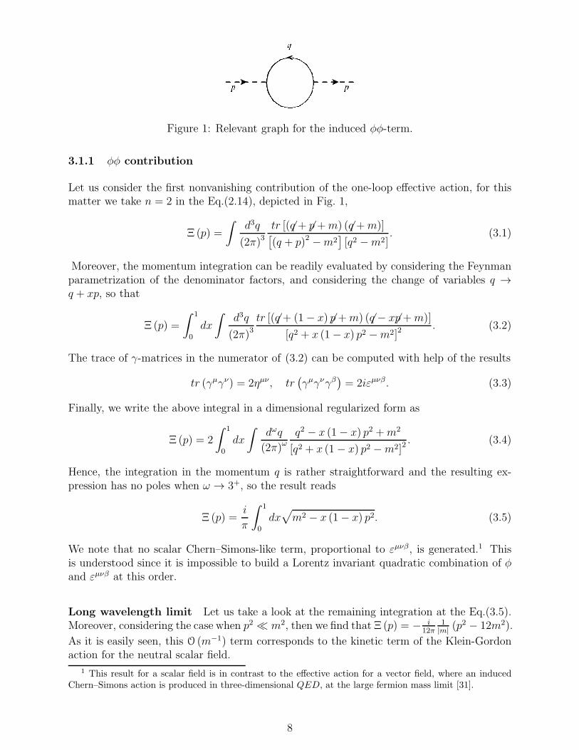
Figure 1: Relevant graph for the induced φφ-term.

3.1.1 φφ contribution

Let us consider the first nonvanishing contribution of the one-loop effective action, for thismatter we take n = 2 in the Eq.(2.14), depicted in Fig. 1,

Ξ (p) =

∫d3q

(2π)3tr [( 6q + 6p+m) ( 6q +m)][(q + p)2 −m2

][q2 −m2]

. (3.1)

Moreover, the momentum integration can be readily evaluated by considering the Feynmanparametrization of the denominator factors, and considering the change of variables q →q + xp, so that

Ξ (p) =

∫ 1

0

dx

∫d3q

(2π)3tr [( 6q + (1− x) 6p+m) ( 6q − x6p+m)]

[q2 + x (1− x) p2 −m2]2. (3.2)

The trace of γ-matrices in the numerator of (3.2) can be computed with help of the results

tr (γµγν) = 2ηµν , tr(γµγνγβ

)= 2iεµνβ. (3.3)

Finally, we write the above integral in a dimensional regularized form as

Ξ (p) = 2

∫ 1

0

dx

∫dωq

(2π)ωq2 − x (1− x) p2 +m2

[q2 + x (1− x) p2 −m2]2. (3.4)

Hence, the integration in the momentum q is rather straightforward and the resulting ex-pression has no poles when ω → 3+, so the result reads

Ξ (p) =i

π

∫ 1

0

dx√m2 − x (1− x) p2. (3.5)

We note that no scalar Chern–Simons-like term, proportional to εµνβ, is generated.1 Thisis understood since it is impossible to build a Lorentz invariant quadratic combination of φand εµνβ at this order.

Long wavelength limit Let us take a look at the remaining integration at the Eq.(3.5).Moreover, considering the case when p2 ≪ m2, then we find that Ξ (p) = − i

12π1|m|

(p2 − 12m2).

As it is easily seen, this O (m−1) term corresponds to the kinetic term of the Klein-Gordonaction for the neutral scalar field.

1 This result for a scalar field is in contrast to the effective action for a vector field, where an inducedChern–Simons action is produced in three-dimensional QED, at the large fermion mass limit [31].

8

Figure 2: Relevant graph for the induced φφφ-term.

In the configuration space, if we replace the above result into the expression (2.13) wefind after some manipulation that

Γ (x1, x2) = −ig2

24π

1

|m|(�+ 12m2

)δ (x1 − x2) . (3.6)

As it is well-known, there is no noncommutativity effects for the case of two fields, since thephase factor in (2.13) vanishes. Finally, the analysis of the first nonvanishing term in (2.12)is given by

iΓ [φφ] =ig2

24π

1

|m|

∫d3x

(∂µφ∂

µφ− µ2φ2)(x) , (3.7)

and it leads to the radiatively induced Klein-Gordon action, where we have introduced anew square mass parameter µ2 = 12m2.

3.1.2 φφφ contribution

The calculation of the next contribution follows as in the previous analysis. We compute then = 3 contribution in the Eq.(2.14) and given in Fig. 2,

Ξ (p, k) =

∫d3q

(2π)3tr [( 6q + 6p+m) (6q +m) ( 6q − 6k +m)][

(q + p)2 −m2][q2 −m2]

[(q − k)2 −m2

] . (3.8)

The momentum integral can be computed straightforwardly using the dimensional regu-larization, and realizing that Γ

(2− ω

2

)and Γ

(3− ω

2

)have no poles when ω → 3+, so we

find

Ξ (p, k) =i

16π

∫dξ

[N1 (p, k; x, z)

(m2 − A2 (p, k))1

2

− N2 (p, k; x, z)

(m2 −A2 (p, k))3

2

], (3.9)

where by simplicity we have defined sµ = xpµ− zkµ , the measure∫dξ =

∫ 1

0dx∫ 1−x

0dz, and

the quantity A2 (p, k) = − (xp− zk)2 + xp2 + zk2, as well as the following quantities

N1 (p, k; x, z) = 3tr (−3 6s− 6k + 6p) + 18m, (3.10)

and

N2 (p, k; x, z) = −tr [( 6s− 6p) ( 6s−m) ( 6s+ 6k −m)] +mtr [( 6s−m) ( 6s+ 6k −m)] . (3.11)

As usual, the full contribution of (3.9) gives rise to a full set of information, but here we areinterested in the particular cases of the O (m0) and O (m−2) contributions, in order to addthese self-interacting terms to the kinetic contribution (3.7).

9

Derivative coupling Although the structure of the contribution (3.9) is rather compli-cated than those from the two fields, we can keep traced of the terms O (m0) and O (m−2)by paying careful attention to the contributions from the numerator and denominator at thelong wavelength limit. For that matter, we shall focus on the O (m1) and O (m3) contribu-tions from the quantities N1 (p, k; x, z) and N2 (p, k; x, z), and take the p2 ≪ m2 limit. Withsuch considerations the remaining integral can now be computed, so that the three fieldscontribution is simply given by

Ξ (p, k) =i

8π

m

|m|

[4 +

1

6m2

(3k2 + 2p2 + 2 (p.k)

)]. (3.12)

Finally, the interacting effective action (2.12) of the noncommutative Klein-Gordon actionfor a neutral scalar field is found to be

iΓ [φφφ] =ig3

6π

m

|m|

∫d3x

(φ ⋆ φ ⋆ φ+

1

3m2∂αφ ⋆ ∂αφ ⋆ φ

)(x) , (3.13)

where we have applied the identity 2∫d3x ∂αφ ⋆ ∂αφ ⋆ φ = −

∫d3x �φ ⋆ φ ⋆ φ, found as

a result of using the cyclic property of the Moyal product and performing an integrationby part. We thus see that a noncommutative λφ3

⋆ interacting term is radiatively generated,in addition to a derivative coupling as well, where the coupling constant has dimension of[λ] = [gm]. It is worth to mention that due to theory’s structure higher self-interactingcontributions λφn

⋆ for n > 3 are absent in the effective action of a neutral scalar field at thelong wavelength limit, even the well-known dimensionless coupling λφ6

⋆. In contrast, we findthat only derivative couplings are present in this situation.

Once again, similarly to the case of φφ contribution, we also see that a Chern–Simons-like term does not appear in the analysis of the φφφ contribution. This can be easily seenby considering the possible Chern–Simons-like expressions described by

∫d3x εµνβ(∂µφ) ⋆

(∂νφ) ⋆ (∂βφ) or∫d3x εµνβ(∂µ∂αφ) ⋆ (∂ν∂

αφ) ⋆ (∂βφ) that are apparently nonzero but are infact both of them vanish, due to the integration by part and discarding the surface terms.

3.2 Charged scalar fields

For completeness, in addition to the discussion of a neutral scalar field, let us consider thecase of charged scalar fields too. The fermionic action in this case is defined as

S =

∫d3x

[iψ ⋆ γµD⋆

µψ −mψ ⋆ ψ + gψ ⋆ Φ ⋆ ψ + h.c.], (3.14)

in which the covariant derivative is defined asD⋆µψ = ∂ψ−ieAµ⋆ψ, and the h.c. term ensures

the reality of the action. Moreover, this action is invariant under the local infinitesimal gaugetransformations,

δψ = igλ ⋆ ψ, δAµ = ∂µλ− ie [Aµ, λ]⋆ . (3.15)

The one-loop effective action coming from (3.14) are readily obtained,

iΓ [A] = −∑

n

1

ntr

(( 6∂ + im)−1i (gφ ⋆+e6A⋆)

)n

, (3.16)

10

Figure 3: Relevant graph for the induced φφA-term.

where we have defined by simplicity the combination φ = Φ + Φ†. The n = 2 contributionis exactly the same as the one obtained in (3.7), just with the previous replacement on thefield φ. We shall now proceed to analyse the interacting terms between the scalar and gaugefields coming from the n = 3 and n = 4 terms.

3.2.1 φφA contribution

Let us start with the first contribution coming from n = 3 and depicted in Fig. 3. Amongall these interacting terms coming from this expansion we shall concentrate in those giving acombination of φφA fields. We thus find that three terms are present and have the followingstructure

iΓ [φφA] ≃∫d3x1d

3x2d3x3

[[φ (x1)φ (x2)Aµ (x3)]Γ

µ

(a) (x1, x2, x3) (3.17)

+ [φ (x1)Aµ (x2)φ (x3)]Γµ

(b) (x1, x2, x3) + [Aµ (x1)φ (x2)φ (x3)]Γµ

(c) (x1, x2, x3)

],

where we define and compute the general tensor quantities Γµ

(i) (x1, x2, x3), for i = a, b, c, inthe Appendix B.

Therefore, substituting the results (B.8) and (B.9) back into the expression (3.17), andafter some straightforward integral manipulation we are finally able to write

iΓ(a) [φφA] =g2e

36π

1

|m|

∫d3x [∂µφ ⋆ φ ⋆ Aµ − φ ⋆ ∂µφ ⋆ Aµ] , (3.18)

iΓ(b) [φφA] = −g2e

36π

1

|m|

∫d3x [∂µφ ⋆ Aµ ⋆ φ− φ ⋆ Aµ ⋆ ∂

µφ] , (3.19)

iΓ(c) [φφA] =g2e

36π

1

|m|

∫d3x [Aµ ⋆ ∂

µφ ⋆ φ− Aµ ⋆ φ ⋆ ∂µφ] . (3.20)

The complete contribution is found by summing the above three contributions, Eqs.(3.18)–(3.20). Thus, using the cyclic property of the Moyal product, we find

iΓ [φφA] = iΓ(a) [φφA] + iΓ(b) [φφA] + iΓ(c) [φφA] ,

=g2e

12π

1

|m|

∫d3x [Aµ ⋆ ∂

µφ ⋆ φ−Aµ ⋆ φ ⋆ ∂µφ] . (3.21)

At last, by using the definition φ→ Φ + Φ† and keeping the relevant terms, we can rewriteexpression (3.21) into the following convenient form

iΓ[ΦΦ†A] ≃ g2e

12π

1

|m|

∫d3x

([Φ†, Aµ

]⋆⋆ ∂µΦ− ∂µΦ† ⋆ [Aµ,Φ]⋆

). (3.22)

11

Figure 4: Relevant graph for the induced φφAA-term.

As we will see afterwards, this result is exactly the cubic interaction from the NC Higgsmodel, since the coupling in this case is given by (DµΦ)

†⋆DµΦ, where the covariant derivativeis now written in its adjoint form DµΦ = ∂µΦ− ie [Aµ,Φ]⋆. It is worth of mention that thegenerated couplings are in the adjoint representation and not in the fundamental one.2

3.2.2 φφAA contribution

By means of complementarity, we now approach the one-loop n = 4 contribution to thecharged scalar fields effective action, which graph is given in Fig. 4, where we shall find thelast piece of the interacting sector.

The contribution proportional to the following structure of φφAA fields is given by sixterms

iΓ [φφAA] ≃∫d3x1 · · · d3x4

[[φ (x1)φ (x2)Aµ (x3)Aν (x4)]Γ

µν

(a) + [φ (x1)Aµ (x2)φ (x3)Aν (x4)]Γµν

(b)

+ [φ (x1)Aµ (x2)Aν (x3)φ (x4)]Γµν

(c) + [Aµ (x1)φ (x2)φ (x3)Aν (x4)]Γµν

(d)

+ [Aµ (x1)φ (x2)Aν (x3)φ (x4)]Γµν

(e) + [Aµ (x1)Aν (x2)φ (x3)φ (x4)]Γµν

(f)

], (3.23)

where we define and compute the tensor quantities to each one of these contributions Γµν

(i)

i = a, b, ..., f , in the Appendix B.

Hence, replacing the results (B.18) in conjunction with (B.11) and (B.12) back into theexpression (3.23), we find out the following

iΓ [φφAA] =i

12π

g2e2

|m|

∫d3x [φ ⋆ Aµ ⋆ A

µ ⋆ φ− φ ⋆ Aµ ⋆ φ ⋆ Aµ] . (3.24)

Now, making use again of φ→ Φ+Φ†, we finally find the expression for the effective action

iΓ[ΦΦ†AA

]=

i

12π

g2e2

|m|

∫d3x

( [Φ†, Aµ

]⋆⋆ [Aµ,Φ]⋆

). (3.25)

As we have anticipated, the expression (3.25) is precisely the last piece for the (minimal)interaction content of the NC Higgs model (DµΦ)

†⋆DµΦ, consisting in the quartic interactionamong the scalar and gauge fields.

2This fact might be closely related to our choice of interaction term in (2.1), perhaps because differentcouplings such as ψ ⋆ ψ ⋆φ or ψ ⋆ [φ, ψ]⋆ could give in principle different contributions to the effective action.However, this fact should be further elaborated and then analysed.

12

Figure 5: One-loop self-energy graph for the neutral scalar field.

4 Propagating modes scalar field

From the obtained results, Eqs.(3.7) and (3.13), we can analyse the dynamics of the scalarfields by proposing the following effective Lagrangian for the noncommutative neutral scalarfield

L =1

2

(∂µφ∂

µφ−m2φ2)+λ

3!

(φ ⋆ φ ⋆ φ+

1

3m2∂µφ ⋆ ∂µφ ⋆ φ

). (4.1)

Notice that the usual φ3⋆ theory is recovered in the limit when the HD contribution decouples.

The Feynman rules for this theory are readily obtained from the Lagrangian (4.1).

Moreover, we can establish the renormalization of the complete propagator, by writingthe self-energy function as Σ (p2) = p2Σ1 (p

2) +m2Σ2 (p2), that can be carried out as

S (p) =1

p2 −m2 − Σ (p2)=

1

p2 (1− Σ1 (p2))−m2 (1 + Σ2 (p2))=

Z

p2 −m2ren

where we have defined the renormalization constants as Z−1 = 1 − Σ1 (p

2) and Z−1m =

1 + Σ2 (p2), so that the renormalized mass is defined as the following

mren = m

√Z

Zm

. (4.2)

Hence, the one-loop self-energy for the neutral scalar fields reads (see Fig. 5)

Σ (p) = −iλ2∫

d3q

(2π)31

q2 −m2

1

(q − p)2 −m2

[1 +

1

9m2

((p.q) + (q − p)2

)]2cos2

[p× q2

],

(4.3)

We can work out the numerator of the above expression in order to simplify the dependenceon the integrated momentum. Furthermore, we now compute separately the planar from thenon-planar contribution by means of the identity 2 cos2[p×Q

2] = 1 + cos (p×Q). First, the

planar contribution results into the following

Σp (p) =1

1296π

λ2

m

{∫ 1

0

dx[100 + 20xβ + x2β2

] 1

(1− x (1− x) β)1

2

+ β

∫ 1

0

dx√

1− x (1− x) β + 2 [20 + β]

}, (4.4)

where we have defined the notation β = p2/m2. Next, the non-planar contribution from

13

(4.3) can be computed with help of the results Eqs.(A.1) and (A.2), and yields

Σn−p (p) =1

1296π

λ2

m

{∫ 1

0

dx[100 + 20xβ + x2β2

] e−m|p|√

1−x(1−x)β

√1− x (1− x) β

− β

m |p|

∫ 1

0

dx e−m|p|√

1−x(1−x)β − 2 [20 + β]1

m |p|e−m|p|

}. (4.5)

Finally, the complete contribution is given by the sum of (4.4) and (4.5), Σ (p) = Σp (p) +Σn−p (p).

Now with the one-loop self-energy we can analyse the renormalized mass expressionstructure. Thus, expanding (4.2) at leading order, we find that

mren = m

√Z

Zm

≃ m+ Σ(1) + O(α2), (4.6)

where we have defined Σ(1) = m2(Σ1 (m

2) + Σ2 (m2)), with the previous coefficients given by

Σ1

(m2)=

1

1296π

λ2

m3

{∫ 1

0

dx[20x+ x2]√1− x (1− x)

[1 + e−m|p|

√1−x(1−x)

]

+

∫ 1

0

dx

[√1− x (1− x)− 1

m |p|e−m|p|√

1−x(1−x)

]+ 2

(1− 1

m |p|e−m|p|

)}. (4.7)

and

Σ2

(m2)=

1

1296π

λ2

m3

{∫ 1

0

dx100√

1− x (1− x)

[1 + e−m|p|

√1−x(1−x)

]+ 40

(1− 1

m |p|e−m|p|

)}.

(4.8)

Hence, we see that the dispersion relation for the scalar field at this order reads

ω2 = ~p2 +m2ren ≃ ~p2 +m2 + 2mΣ(1) + O

(α2). (4.9)

By means of illustration, we shall consider the infinitesimal noncommutative modification inthe dispersion relation. Thus, if we additionally take the on-shell limit, i.e. |p| = |θ|

√p2 →

m |θ|, we can write the dispersion relation in the following simple form

ω2 ≃ ~p2 +m2 +1

1296π

λ2

m

(86 +

441

2log 3

)− 43

1296π

λ2

m3θ+ O

(λ2θ). (4.10)

Immediately we observe two features from the expression (4.10). First, we find a correction

for the mass asm2eff = m2

[1 + λ2

πm3

(43648

+ 49288

log 3)], meaning that the particle gets heavier.

Second, the last term shows the presence of a UV/IR instability (with a 1/θ behavior) causedby noncommutative perturbative effects.

5 Propagating modes charged scalar fields

In addition, we now consider the obtained results (3.22) and (3.25) (the gauge field effectiveaction was obtained in [31]), so that we can propose the following effective Lagrangian for

14

Figure 6: One-loop self-energy graphs for the charged scalar field: (a) cubic interactioncontribution, (b) quartic interaction contribution.

the charged scalar fields coupled with a higher derivative Chern-Simons field

L = (DµΦ)† ⋆DµΦ−m2Φ† ⋆ Φ +

m

2εµνσAµ

(1 +

�

m2

)∂νAσ

− 1

2ξ(∂µA

µ)2 +me

3εµνσAµ ⋆ Aν ⋆ Aσ + ∂µc ⋆ Dµc, (5.1)

where the covariant derivatives are defined as such Dµ = ∂µ − ie [Aµ, ]⋆. Based on theLagrangian (5.1) we will study the dynamics of the scalar and gauge fields.

Notice that the model described by the Lagrangian (5.1) has a non-gauge invariant contri-bution, given by the higher derivative (HD) term. The generation of higher derivative termsand derivative couplings within the NC Chern-Simons theory were considered in Ref. [31]Moreover, our interest in exploring the features of this HD term into the propagator is moti-vated by the possibility of finding non-trivial effects into the whole NC Chern-Simons-Higgstheory (5.1). For instance, as we will shortly show (see Sect.5.2) this solely HD contribu-tion is responsible for obtaining nontrivial outcomes for the pure NC CS theory (which isa free theory without the HD term), so its effect on the complete theory is expected to berather interesting. Moreover, it is easy to see that the commutative limit of this NC HDChern-Simons theory is also a free theory.

We shall now approach two physical situations in the NC HD-Chern-Simons-Higgs theory:we consider first the dispersion relation of the scalar fields, where the two-point functionrenormalization takes place as before; second, we analyse the dispersion relation for thegauge field.

5.1 Dispersion relation charged scalar fields

For the one-loop self-energy contribution, we have the following two diagrams (Fig. 6), thewhole contribution reads

Σ (p) = Σ(a) (p) + Σ(b) (p) ,

=(√

2)2ie2∫

d3q

(2π)3iDµν (q)

[(2p− q)µ (2p− q)ν

(q − p)2 −m2− 2ηµν

]sin2

[p× q2

]. (5.2)

An important remark follows from (5.2), we observe that only the symmetric part of thegauge field propagator

iDµν (k) = miεµνσk

λ

k2 (k2 −m2)+ ξ

kµkνk4

. (5.3)

15

contributes at this perturbative order. Hence, only a non-physical gauge-dependent contri-bution is present in the case of a Chern-Simons gauge field. By completeness, we will discussbelow the result for the NC Maxwell-Chern-Simons theory.

Nonetheless, making use of the propagator (5.3) and rewriting (5.2) with help of Feynmanparametrization, we obtain

Σ (p) = 2iξe2µ3−ω

∫dωQ

(2π)ω

[8

∫ 1

0

dx (1− x)((p.Q)2 + x2p4

) 1

(Q2 + x (1− x) p2 − xm2)3

− 4

∫ 1

0

dxxp2

(Q2 + x (1− x) p2 − xm2)2+

1

Q2 −m2− 2

Q2

]sin2

[p×Q2

]. (5.4)

Now, it is convenient to compute separately the planar from the non-planar contributionsfrom (5.4), this is achieved by means of 2 sin2[p×Q

2] = 1−cos (p×Q). We have, for the planar

contribution

Σp (p) = −ξe2m

8π

[2β

∫ 1

0

dx (1− x)[

1

(x− x (1− x) β)1

2

− x2β 1

(x− x (1− x) β)3

2

]

− 4β

∫ 1

0

dx x1

(x− x (1− x) β)1

2

+ 2

], (5.5)

whereas, with help of (A.1) and (A.2), the non-planar contribution reads

Σn−p (p) =ξe2m

4π

[−2β

∫ 1

0

dxxe−m|p|

√x−x(1−x)β

√x− x (1− x) β

− 1

m |p|e−m|p| +

2

m |p|

+ β

∫ 1

0

dx (1− x)

1− x2β

(1 +m |p|

√x− x (1− x) β

)

(x− x (1− x) β)

e−m|p|

√x−x(1−x)β

√x− x (1− x) β

].

(5.6)

The renormalization here follows closely the steps as of the neutral scalar field, so that therenormalized mass is also given by (4.2). Hence, we can proceed and decompose the one-loop self-energy in terms of its components, Σ (p2) = p2Σ1 (p

2) +m2Σ2 (p2). Now, since the

renormalization is performed on-shell, we have that these components are simply written as

Σ1(m2) = −ξe

2

4π

1

m

[1

m |p| − 1− e−m|p|

m |p|

], (5.7)

Σ2(m2) = −ξe

2

4π

1

m

[1 +

1

m |p|e−m|p| − 2

m |p|

]. (5.8)

As we have already discussed, the renormalized mass is given by (4.2) mren = m√

1+Σ2(m2)1−Σ1(m2)

,

so the dispersion relation for the charged scalar fields are written as

ω2 = ~p2 +m2ren ≃ ~p2 +m2 +m2

(Σ1(m

2) + Σ2(m2))+ O

(α2). (5.9)

Finally, making use of (5.7) and (5.8), and recalling that at the on-shell limit we have|p| → m |θ|, we thus find

ω2 ≃ ~p2 +m2 +ξe2

4π

1

mθ+ O

(e2θ). (5.10)

16

Some conclusions can be depicted from the expression (5.10). We first realize that in thisframework no radiative correction for the mass is found. However, we still have a UV/IRinstability caused by NC effects, in particular we see that this UV/IR instability is propor-tional to the gauge parameter ξ, and for the Landau gauge, this instability vanishes. Wetherefore conclude that this sector of the theory is empty of physical content.

In order to illustrate the physical content of the scalar sector, let us consider the usualMaxwell-Chern-Simons propagator (at Landau gauge, ξ = 0)3

iDµν (k) =1

k2 (k2 −m2)

(k2ηµν − kµkν + imεµνλk

λ), (5.11)

this gives the following expression for the scalar field dispersion relation

ω2 ≃ ~p2 +m2 − e2m

π

(1 +

e−m2θ

m2θ

)+ O

(e2θ), (5.12)

where we realize that in this framework of a Maxwell-Chern-Simons gauge field, a radiativecorrection for the mass of the scalar field is found, so that the effective mass reads m2

eff =

m2[1− 1

πe2

m

]. In the same way, we also have a UV/IR instability caused by NC effects. All

these effects present in (5.12) are caused by the symmetric component of the propagator(5.11).

5.2 Dispersion relation gauge field

In general, we can consider that the self-energy 1PI-function in a three dimensional non-commutative spacetime has the following tensor form [29]

Πµν =

(ηµν − pµpν

p2

)Πe +

pµpν

p2Πe + iΠA

0 ǫµνλpλ +ΠS

0

(pµuν + pνuµ

), (5.13)

where we regard the basis composed by the vectors pµ, pµ and uµ = ǫµαβpαpβ; moreover, the

form factors Πe, Πe, ΠA

0 and ΠS

0 are determined by means of the following relations

Πe =ηµνΠµν − pµpν

p2Πµν , (5.14)

Πe =− ηµνΠµν + 2pµpνp2

Πµν , (5.15)

ΠA

0 =i

2p2ǫµναp

αΠµν , (5.16)

ΠS

0 =−1

2p4p2(uµpν + uνpµ)Π

µν . (5.17)

3This is justifiable as an example, since we have a symmetric operator multiplying the gauge field propa-gator in (5.2), so the skew-symmetric nature of the pure Chern-Simons propagator gives a vanishing result.

17

Figure 7: One-loop self-energy graphs for the gauge field: (a) scalar loop, (b) scalar tadpoleloop, (c) gauge loop, (d) ghost loop.

Moreover, the general expression of the complete propagator for the CS gauge field (aug-mented with the HD term) can be put into the form [29]

iDµν = −Πe + Πe

Dηµν +

(Πe + Πe

D+

ξ

p2

)pµpνp2

+Πe

D

pµpνp2

+ΠS

0

D(pµuν + uµpν) +

m(1− p2

m2

)+ΠA

0

Diεµνλp

λ. (5.18)

where by simplicity we have defined the quantity at the denominator

D = Πe

(Πe + Πe

)+ p2

[(p2ΠS

0

)2 −(m

(1− p2

m2

)+ΠA

0

)2]. (5.19)

Before discussing the structure of the complete propagator we shall now compute the one-loop contribution to the polarization tensor.

The one-loop correction to the gauge field self-energy is given by the four contributionsdepicted in Fig. 7: the first and second contributions are from the scalar loops, graph (a)corresponds to the scalar loop , while graph (b) to the scalar tadpole loop , graph (c)corresponds to the gauge loop , and graph (d) corresponds to the ghost loop, respectively.Their explicit expressions are written as

Π(a+b)µν (p) = −2ie2

∫d3q

(2π)31

q2 −m2

[(2q − p)µ (2q − p)ν

(q − p)2 −m2− 2ηµν

]sin2

[p× q2

], (5.20)

Π(c)µν (p) = −im4e2

∫d3q

(2π)3qν (q − p)µ + qµ (q − p)ν

(q − p)2((q − p)2 −m2

)q2 (q2 −m2)

sin2

[p× q2

], (5.21)

Π(d)µν (p) = 2ie2

∫d3q

(2π)31

q2(q − p)µ qν(q − p)2

sin2

[p× q2

]. (5.22)

In the first line, by simplicity of notation, we have summed the two contributions comingfrom the scalar loops.

An interesting remark is now in place. In particular, in the limit m → ∞, that cor-responds to the situation where the HD contribution is removed, we find that the scalarcontributions (5.20) are equal to zero, while the contributions (5.21) and (5.22) sum to

Π(c+d)µν (p) = ie2

∫ 1

0

dy

∫d3Q

(2π)3[Qνpµ − pνQµ]

[Q2 + yp2]2sin2

[p×Q2

]= 0. (5.23)

18

This is a known result where we see that the NC Chern-Simons theory is a free theory [24].However, we conclude that the HD contributions are sufficient to modify the character of thepolarization tensor of the pure NC Chern-Simons theory, rendering a nonvanishing result.

Moreover, in order to evaluate the form factors (5.14)–(5.17) it is easier to compute thecontraction of the expressions (5.20)–(5.22) with the operators ηµν , pµpν/p2, εµνλpλ, and(uµpν + uν pµ). Surprisingly, we immediately find out that the following projections

(uµpν + uνpµ)Π(a+b)µν = (uµpν + uνpµ)Π(c)

µν = (uµpν + uν pµ)Π(d)µν = 0, (5.24)

and

εµνλpλΠ(a+b)µν = εµνλpλΠ

(c)µν = εµνλpλΠ

(d)µν = 0, (5.25)

vanish identically. In particular, we have made use of the identities p.u = 0 and p.p = 0in order to obtain the previous results. So, the form factors ΠA

0 and ΠS

0, Eqs.(5.16) and(5.17), respectively, vanish at this order. Hence, we are left to compute only the projectionof (5.20)–(5.22) onto the operators ηµν and pµpν/p2.

The planar and non-planar parts of the contractions ηµνΠµν (p) andpµpν

p2Πµν (p) are com-

puted in the Appendix C.

Before computing the form factors Πe and Πe, Eqs.(5.14) and (5.15), respectively, let usnow establish the renormalizability of the theory. First, note that due to the fact that theform factors ΠA

o and ΠSo are null, the expression of the complete propagator (5.18) reads

iDµν = −Πe + Πe

Dηµν +

(Πe + Πe

D+

ξ

p2

)pµpνp2

+Πe

D

pµpνp2

+m(1− p2

m2

)

Diεµνλp

λ, (5.26)

with a simplified form D = Πe(Πe+Πe)−p2m2(1− p2

m2

)2. It is sufficient for our interest, in

defining the physical pole of the NC HD Chern-Simons sector, to consider the CP odd termfrom (5.26)

iDµν ∼m(1− p2

m2

)

p2[p2Πe(Πe + Πe)−m2

(1− p2

m2

)2] iεµνλpλ, (5.27)

where we have performed the scaling{Πe, Πe

}→ p2

{Πe, Πe

}. By a simple analysis and

manipulation we can rewrite the expression (5.27) in its renormalized form

iDµν ∼mrenZCP

p2 [p2 −m2ren]

iεµνλpλ, (5.28)

where the physical pole p2 = m2ren is localized so that the renormalized mass of the Chern-

Simons gauge field and the respective renormalization constant were defined as

mren = ZCPm, Z

CP=

1√1 + Πe

(Πe + Πe

) . (5.29)

19

In order to finally compute the renormalized mass, it is worth to evaluate the form factorsΠe and Πe in the highly noncommutative limit, i.e. β = p2/m2 → 0 while k2 is kept finite.This allows us to obtain the leading noncommutative effects onto the renormalized mass.

Hence, from the expression (5.14) we find that

Πe (p) = ηµνΠµν(p)− pµpν

p2Πµν(p)

=e2

12π

1

m2|p|3{3 (2 +m|p|)2 e−m|p| −

(12 +m3|p|3

)}. (5.30)

Moreover, due to the structure of the renormalization constant ZCP

in (5.29), it showsconvenient to compute the following combination

Πe + Πe =pµpνp2

Πµν(p)

= − e2

24π

1

m2|p|3{−24 +m3|p|3 + 3

(8 + 8m|p|+ 8m2p2 + 5m3|p|3

)e−m|p|

}. (5.31)

We can finally make use of the results (5.30) and (5.31) into the expression (5.29) inorder to compute the renormalized mass

mren ≃ m− 1

16π2

1

κ2m|p|2 +5

32π2

1

κ2|p| −1

8π2

m

κ2+ O

(m|p|κ

), (5.32)

when writing this expression we have used the tree-level relation e2 ∼ m/κ. Moreover, wesimplified the above terms by taking the leading noncommutative perturbations m|p| ≪ 1.Furthermore, recalling that at the on-shell limit we have |p| → m |θ|, the dispersion relationfor the Chern-Simons gauge field reads

ω2 ≃ |~p|2 +m2 − 1

4π2

m2

κ2− 1

8π2

1

κ2m2

1

θ2+

5

16π2

1

κ21

θ+ O

(m2θ

κ

). (5.33)

In particular, we see that a correction is obtained for the massive mode,m2eff = m2

[1− 1

4π2

1κ2

],

and that a leading 1/θ2 and subleading 1/θ UV/IR mixing are present in this case.

6 Concluding remarks

In this paper we have considered the Yukawa field theory for neutral and charged scalar fieldsin the framework of a noncommutative three-dimensional spacetime. In order to study thedynamics of the scalar fields we have followed the effective action approach by integratingout the fermionic fields. The two-point function renormalization for both cases were carefullyestablished, allowing us to define the physical dispersion relation and hence study the UV/IRanomaly.

Initially we established the main properties of the effective action approach for noncom-mutative field theories [31,39]. In particular, we defined the noncommutative Yukawa actionfor a neutral scalar field and computed its effective action, and showed that besides its kineticterms, only a cubic interaction φ3

⋆ is present at the leading order O(m0), and that φn⋆ (for

20

n > 3) interacting terms are absent in its effective action when defined in a three-dimensionalspacetime. Additionally, we considered the case of charged scalar fields, where a gauge fieldis need in order to ensure a local gauge invariance. Hence, by computing the respectivecubic and quartic terms, we found the minimal interacting parts of the NC Higgs model, i.e.charged scalar fields minimally coupled to a gauge field.

In order to illustrate the behavior of the neutral scalar field in a noncommutative three-dimensional spacetime, we considered the effective action with an additional derivative cou-pling supplementing the cubic interacting term. We then determined the respective Feynmanrules and the one-loop correction to the self-energy, also the renormalized mass was estab-lished. After computing the planar and non-planar contributions to the one-loop self-energywe found the physical dispersion relation, where we have showed a correction to the baremass and the presence of a 1/θ singular term, as a result of UV/IR instability caused bynoncommutative effects.

By completeness, we considered the effective action for charged scalar fields coupled witha dynamical Chern-Simons gauge field. We have considered a higher-derivative contributionto the kinetic term of the gauge field in order to discuss some novel features in the gauge fieldsector. By computing first the one-loop correction to the scalar field self-energy, we showedthat this contribution is non-physical due to its dependence on the gauge parameter ξ ontothe dispersion relation; by means of illustration we presented how the dispersion relation ismodified and became physical if a Maxwell-Chern-Simons propagator is considered insteadof the HD-Chern-Simons propagator. Afterwards, we established the renormalization andanalysed the one-loop dispersion relation for the gauge field. In the resulting expression wefound the presence of a correction to the bare mass parameter, and that a leading 1/θ2 andsubleading 1/θ UV/IR mixing are present in this case.

It is worth of mention that all the previous analysis were considered in the highly noncom-mutative limit of the Chern-Simons-Higgs theory, that also corresponds to the low-momentalimit. As we have discussed, this kind of effective models are nowadays of major interestfor physical application in planar materials, in particular in the description of new materialsin the framework of condensed matter physics, which allows the use of effective low-energymodels. Moreover, this model can be an appropriate field-theoretical framework for study ofAharonov-Bohm effect. This framework also works in a way to provide a consistent scenarioto scrutinize theoretical features in order to set stringent bounds on deviations of knownfield theory properties, for instance standard model symmetries.

Acknowledgements

We would like to thank M.M. Sheikh-Jabbari for discussion. R.B. thankfully acknowledgesCAPES/PNPD for partial support, Project No. 23038007041201166.

A Non-planar integrals

Along the paper we have made use of some results involving momentum integration. Weshall recall some of these results, in particular those involving a non-planar factor. The

21

simplest non-planar integration reads

∫dωq

(2π)ω1

(q2 − s2)a eik∧q =

2i (−)a

(4π)ω2

1

Γ (a)

1

(s2)a−ω2

(|k|s2

)a−ω2

Ka−ω2

(|k|s). (A.1)

Next, we have the tensor integration

∫dωq

(2π)ωqµqν

(q2 − s2)a eik∧q = ηµνFa +

kµkν

k2Ga, (A.2)

where we have introduced the following quantities

{Fa, Ga} =i (−)a−1

(4π)ω2

1

Γ (a)

1

(s2)a−1−ω2

{fa, ga} , (A.3)

with

fa =

(s|k|2

)a−1−ω2

Ka−1−ω2

(|k|s), (A.4)

ga = (2a− 2− ω)(s|k|2

)a−1−ω2

Ka−1−ω2

(|k|s)− 2

(s|k|2

)a−ω2

Ka−ω2

(|k|s). (A.5)

B Effective action

We summarize in this appendix some useful and important long expressions related to thecomputation of the effective action in the Sec. 3.

B.1 φφA contribution

The three distinct contributions for the one-loop effective action for the φφA vertex (3.17)are given by

Γµ

(i) (x1, x2, x3) =g2e

3

∫d3p1

(2π)3d3p2

(2π)3d3p3

(2π)3[(2π)3 δ (p1 + p2 + p3)

]exp [−i (p1.x1 + p2.x2 + p3.x3)]

× exp

[− i2(p1 × p2 + p1 × p3 + p2 × p3)

]Ξµ

(i) (p1, p2) , (B.1)

in which p × q = θµνpµqν , where the explicit expressions Ξµν

(i) are readily obtained from thegraph Fig. 3.

Due to the structure of the momentum integral, and our interest in finding the leadingcontribution for the interaction terms, we see that those correspond to the overall O (m−1)terms, that are precisely the O (m2) and O (m0) terms in the numerator of these expressions,that will result in a (linear) derivative coupling. Hence, from the denominator of the above

22

expressions we find that

tr [...]a ≃ 2m2 (p− k − 3s)µ +2

ωq2 (3p− 3k − 5s)µ , (B.2)

tr [...]b ≃ 2m2 (p− k − 3s)µ − 2

ωq2 (3k + 5s+ p)µ , (B.3)

tr [...]c ≃ 2m2 (p− k − 3s)µ +2

ωq2 (k + 3p− 5s)µ , (B.4)

where we have used the identity qµqν → 1ωq2ηµν . Therefore, with such considerations we can

compute the momentum integration straightforwardly, and by realizing that Γ(2− ω

2

)and

Γ(3− ω

2

)have no poles when ω → 3+, we obtain

Ξµ

(a) (p, k) =i

8π

∫dξ

[(3p− 3k − 5s)µ

(m2 − A2 (p, k))1

2

−m2 (p− k − 3s)µ

(m2 − A2 (p, k))3

2

], (B.5)

Ξµ

(b) (p, k) =i

8π

∫dξ

[− (3k + 5s+ p)µ

(m2 − A2 (p, k))1

2

−m2 (p− k − 3s)µ

(m2 −A2 (p, k))3

2

], (B.6)

Ξµ

(c) (p, k) =i

8π

∫dξ

[(k + 3p− 5s)µ

(m2 − A2 (p, k))1

2

−m2 (p− k − 3s)µ

(m2 − A2 (p, k))3

2

]. (B.7)

Finally, we can now determine the leading contributions by taking the long wavelength limit,i.e. the approximation m2 ≫ A2 (p, k) in the above expressions. Hence, proceeding with thiscalculation and computing the remaining integration, we find

Ξµ

(a) (p, k) ≃i

12π

1

|m| (p− k)µ , Ξµ

(b) (p, k) ≃ −i

12π

1

|m| (k + 2p)µ , (B.8)

Ξµ

(c) (p, k) ≃i

12π

1

|m| (2k + p)µ . (B.9)

B.2 φφAA contribution

The contribution proportional to the structure of the φφAA vertex (3.23) is given by sixterms which has the general structure

Γµν

(i) (x1, x2, x3, x4) = −g2e2

4

∫d3p1

(2π)3· · · d

3p4

(2π)3(2π)3 δ (p1 + p2 + · · ·+ p4) (B.10)

× exp [−i (p1.x1 + · · ·+ p4.x4)] exp

(− i

2

∑

i<j

pi × pj)Ξµν

(i) (p1, p2, p3) ,

where the integral expressions Ξµν

(i) are readily obtained from the graph Fig. 4.

It should be remarked that due to our interest in obtaining the last piece of the (minimal)coupling between scalar and gauge fields, we shall now concentrate in those contributionsindependent of the external momenta in order to complete the derivation of the effectiveaction. In this way, it is easy to show the following equality among the contributions

Ξµν

(a) (p, k, r) = Ξµ

(c) (p, k, r) = Ξµν

(d) (p, k, r) = Ξµν

(f) (p, k, r) , (B.11)

Ξµν

(b) (p, k, r) = Ξµν

(e) (p, k, r) , (B.12)

23

where we find that

Ξµν

(a) (p, k, r) ≃ Γ (4)

∫dζ

∫d3q

(2π)3tr [( 6q +m) ( 6q +m) ( 6q +m) γµ ( 6q +m) γν ]

[q2 +M2 −m2]4, (B.13)

Ξµν

(b) (p, k, r) ≃ Γ (4)

∫dζ

∫d3q

(2π)3tr [( 6q +m) ( 6q +m) γµ ( 6q +m) ( 6q +m) γν ]

[q2 +M2 −m2]4, (B.14)

with the following definition∫dζ =

∫ 1

0

dx

∫ 1−x

0

dz

∫ 1−x−z

0

dw,

M2 (p, k, r) = − (xp− (z + w) k − wr)2 + xp2 + zk2 + w (r + k)2 . (B.15)

Now the numerator of both expressions can be computed with help of the results qµqν →1ωq2ηµν and qµqνqσqρ → 1

ω(ω+2)(q2)

2(ηµνησρ + ηµσηνρ + ηµρηνσ). The resulting expressions

are

tr [...]a = − 10

ω (ω + 2)

(q2)2ηµν + 12m2 1

ωq2ηµν + 2m4ηµν , (B.16)

tr [...]b =30

ω (ω + 2)

(q2)2ηµν + 4m2 1

ωq2ηµν + 2m4ηµν . (B.17)

Once again we see that the momentum integration is finite, since Γ(2− ω

2

), Γ(3− ω

2

)and

Γ(4− ω

2

)have no poles when ω → 3+. Hence, the analysis follows as before, and considering

the expansion m2 ≫ M2 (p, k, r), we find that the leading contributions from Eqs.(B.13) and(B.14) at the O (m−1) terms are

Ξµν

(a) (p, k, r) ≃ −i

12π

1

|m|ηµν , Ξµν

(b) (p, k, r) ≃i

6π

1

|m|ηµν . (B.18)

C Dispersion relation

Therefore, we can compute with no problems the contraction of (5.20)–(5.22) to the operatorsηµν , resulting the total contribution projection

ηµνΠµν (p) = 2ie2µ3−ω

∫dωq

(2π)ω

{−m4 1

q2 (q2 −m2)((q − p)2 −m2

)

−m4 p. (q − p)q2 (q − p)2 (q2 −m2)

((q − p)2 −m2

) + 1

q2+

p. (q − p)q2 (q − p)2

− (2q − p)2

(q2 −m2)((q − p)2 −m2

) + 2ω1

q2 −m2

}sin2

[p× q2

]. (C.1)

while the projection pµpν

p2Πµν yields the contribution

pµpν

p2Πµν (p) = 2ie2µ3−ω p

µpν

p2

∫dωq

(2π)ω

{−m4 qµqν

q2 (q − p)2 (q2 −m2)((q − p)2 −m2

)

+1

q2qµqν

(q − p)2− 4

qµqν

(q2 −m2)((q − p)2 −m2

) + 2ηµν

q2 −m2

}sin2

[p× q2

]. (C.2)

24

Let us now compute separately the planar contribution from the non-planar one of the aboveprojections, this is achieved by the identity 2 sin2[p×Q

2] = 1− cos (p×Q). First, by following

the previous procedure to compute the momentum integration, we find for the planar partof (C.1) and (C.2) the following expressions

(ηµνΠµν)p (p) = −e2m

8π

{1

2

∫ 1

0

dz

∫ 1−z

0

dx1

((1− x)− z (1− z) β)3

2

+3

4β

∫ 1

0

dz

∫ 1−z

0

dx

∫ 1−z−x

0

dw(x+ z)

∆5− β

∫ 1

0

dyy1√

−y (1− y)β

−∫ 1

0

dy

[12√1− y (1− y)β + (2y − 1)2 β

1√1− y (1− y)β

]+ 12

}, (C.3)

and(pµpν

p2Πµν

)

p

=e2m

8π

{−14

∫ 1

0

dz

∫ 1−z

0

dw

∫ 1−z−w

0

dx1

∆3

−∫ 1

0

dy√−y (1− y)β + 4

∫ 1

0

dy√1− y (1− y)β − 4

}, (C.4)

where we have introduced the notation ∆2 = (z + w) − (x+ w) (1− (x+ w))β, and againβ = p2/m2. Next, we compute the non-planar contributions with help of the identities (A.1)and (A.2),

(ηµνΠµν)n−p(p) =

e2m

16π

{∫ 1

0

dz

∫ 1−z

0

dxe−m|p|

√(1−x)1−z(1−z)β

((1− x)− z (1− z) β)3

2

(1 +m|p|

√(1− x)− z (1− z) β

)

+1

2β

∫ 1

0

dz

∫ 1−z

0

dx

∫ 1−z−x

0

dw(x+ z)

∆5

(3 + 3∆m|p|+∆2m2p2

)e−∆m|p|

− 2β

∫ 1

0

dyye−m|p|

√−y(1−y)β

√−y (1− y)β

− 8

∫ 1

0

dy

[√1− y (1− y)β − 2

1

m|p|

]e−m|p|

√1−y(1−y)β

− 2β

∫ 1

0

dy (2y − 1)2e−m|p|

√1−y(1−y)β

√1− y (1− y)β

− 4

m|p|(6e−m|p| + 1

)}, (C.5)

and(pµpν

p2Πµν

)

n−p

=e2m

8π

{1

4

∫ 1

0

dz

∫ 1−z

0

dw

∫ 1−z−w

0

dx[1 + ∆m|p| −∆2m2p2

] e−∆m|p|

∆3

+

∫ 1

0

dy√−y (1− y)β e−m|p|

√−y(1−y)β

− 4

∫ 1

0

dy√1− y (1− y)β e−m|p|

√1−y(1−y)β − 4

m|p|e−m|p|

}. (C.6)

References

[1] H. Yukawa, “On the Interaction of Elementary Particles I,” Proc. Phys. Math. Soc.Jap. 17, 48 (1935).

25

[2] C. M. G. Lattes, H. Muirhead, G. P. S. Occhialini and C. F. Powell, “Processes InvolvingCharged Mesons,” Nature 159, 694 (1947).

[3] G. Amelino-Camelia, “Quantum-Spacetime Phenomenology,”Living Rev. Rel. 16, 5 (2013), arXiv:0806.0339 [gr-qc]

[4] S. Hossenfelder, “Minimal Length Scale Scenarios for Quantum Gravity,”Living Rev. Rel. 16, 2 (2013), arXiv:1203.6191 [gr-qc]

[5] M. R. Douglas and N. Nekrasov, “Noncommutative field theory”,Rev. Mod. Phys. 73, 977 (2001), arXiv:hep-th/0106048;

R. J. Szabo, “Quantum field theory on noncommutative spaces,”Phys. Rept. 378, 207 (2003), arXiv:hep-th/0109162.

[6] I. Hinchliffe, N. Kersting and Y. L. Ma, “Review of the phenomenology of noncommu-

tative geometry,” Int. J. Mod. Phys. A 19, 179 (2004), arXiv:hep-ph/0205040.

[7] P. Nicolini, “Noncommutative Black Holes, The Final Appeal To Quantum Gravity: A

Review,” Int. J. Mod. Phys. A 24 (2009) 1229, arXiv:0807.1939 [hep-th].

[8] M. Chaichian, P. Presnajder, M. M. Sheikh-Jabbari and A. Tureanu, “Non-commutative standard model: Model building,” Eur. Phys. J. C 29 (2003) 413,arXiv:hep-th/0107055.

[9] G. Amelino-Camelia, “Challenge to Macroscopic Probes of Quantum Space-time Based on Noncommutative Geometry,” Phys. Rev. Lett. 111 (2013) 101301,arXiv:1304.7271 [gr-qc].

[10] S. Doplicher, K. Fredenhagen and J. E. Roberts, “Space-time quantization induced byclassical gravity,” Phys. Lett. B 331 (1994) 39.

[11] D. V. Ahluwalia, “Quantum measurements, gravitation, and locality,”Phys. Lett. B 339 (1994) 301 arXiv:gr-qc/9308007.

[12] N. L. Balazs and B. K. Jennings, “Wigner’s function and other distribution functionsin mock phase spaces,” Phys. Rep. 104 (1984) 347.

[13] S. Minwalla, M. Van Raamsdonk and N. Seiberg, “Noncommutative perturbative dy-namics,” JHEP 0002 (2000) 020, arXiv:hep-th/9912072.

[14] D. D’Ascanio, P. Pisani and D. V. Vassilevich, “Renormalization on noncommutativetorus,” Eur. Phys. J. C 76 (2016) no.4, 180 arXiv:1602.01479 [hep-th].

[15] P. Vitale and J. C. Wallet, “Noncommutative field theories on R3λ: Toward

UV/IR mixing freedom,” JHEP 1304 (2013) 115, Addendum: JHEP 1503 (2015) 115arXiv:1212.5131 [hep-th].

[16] A. Gr, T. Juri and J. C. Wallet, “Noncommutative gauge theories on R3λ : perturbatively

finite models,” JHEP 1512 (2015) 045 arXiv:1507.08086 [hep-th].

26

[17] D. N. Blaschke, E. Kronberger, A. Rofner, M. Schweda, R. I. P. Sedmik and M. Wohlge-nannt, “On the Problem of Renormalizability in Non-Commutative Gauge Field Models:A Critical Review,” Fortsch. Phys. 58 (2010) 364 arXiv:0908.0467 [hep-th].

[18] S. Deser, R. Jackiw and S. Templeton, “Topologically Massive GaugeTheories,” Annals Phys. 140 (1982) 372, [Annals Phys. 185 (1988) 406]Annals Phys. 281 (2000) 409.

[19] L. Susskind, “The Quantum Hall fluid and noncommutative Chern-Simons theory,”arXiv:hep-th/0101029.

[20] C. Bastos, O. Bertolami, N. C. Dias and J. N. Prata, “Noncommutative Graphene,”Int. J. Mod. Phys. A 28 (2013) 1350064, arXiv:1207.5820 [hep-th].

[21] B. G. Sidharth, “Graphene and high energy physics,”Int. J. Mod. Phys. E 23 (2014) 5, 1450025.

[22] G. H. Chen and Y. S. Wu, “One loop shift in noncommutative Chern-Simons coupling,”Nucl. Phys. B 593 (2001) 562, arXiv:hep-th/0006114.

[23] A. A. Bichl, J. M. Grimstrup, V. Putz and M. Schweda, “Perturbative Chern-Simonstheory on noncommutative R**3,” JHEP 0007 (2000) 046, arXiv:hep-th/0004071.

[24] A. K. Das and M. M. Sheikh-Jabbari, “Absence of higher order corrections to noncom-mutative Chern-Simons coupling,” JHEP 0106 (2001) 028, arXiv:hep-th/0103139.

[25] M. M. Sheikh-Jabbari, “A Note on noncommutative Chern-Simons theories,”Phys. Lett. B 510 (2001) 247, arXiv:hep-th/0102092.

[26] R. Banerjee, T. Shreecharan and S. Ghosh, “Three dimensional noncommutativebosonization,” Phys. Lett. B 662 (2008) 231, arXiv:0712.3631 [hep-th].

[27] E. A. Asano, L. C. T. Brito, M. Gomes, A. Y. Petrov and A. J. da Silva, “Con-sistent interactions of the 2+1 dimensional noncommutative Chern-Simons field,”Phys. Rev. D 71 (2005) 105005, arXiv:hep-th/0410257.

[28] S. Ghosh, “Bosonization in the noncommutative plane,” Phys. Lett. B 563 (2003) 112arXiv:hep-th/0303022.

[29] M. Ghasemkhani and R. Bufalo, “Noncommutative Maxwell-Chern-Simons the-ory: One-loop dispersion relation analysis,” Phys. Rev. D 93 (2016) no.8, 085021arXiv:1512.04094 [hep-th].

[30] R. Bufalo, T. R. Cardoso and B. M. Pimentel, “Kallen-Lehmann representationof noncommutative quantum electrodynamics,” Phys. Rev. D 89 (2014) 8, 085010arXiv:1404.0941 [hep-th].

[31] R. Bufalo and M. Ghasemkhani, “Higher derivative Chern-Simons extension in the non-commutative QED3,” Phys. Rev. D 91 (2015) 12, 125013, arXiv:1412.1635 [hep-th].

[32] A. F. Ferrari, M. Gomes, J. R. Nascimento, A. Y. Petrov, A. J. da Silva and E. O. Silva,“On the finiteness of the noncommutative supersymmetric Maxwell-Chern-Simons the-ory,” Phys. Rev. D 77 (2008) 025002, arXiv:0708.1002 [hep-th].

27

[33] P. K. Panigrahi and T. Shreecharan, “Induced magnetic moment in noncommutativeChern-Simons scalar QED,” JHEP 0502 (2005) 045, arXiv:hep-th/0411132.

[34] D. N. Blaschke, S. Hohenegger and M. Schweda, “Divergences in non-commutativegauge theories with the Slavnov term,” JHEP 0511 (2005) 041, arXiv:hep-th/0510100.

[35] C. P. Martin, D. Sanchez-Ruiz and C. Tamarit, “The Noncommutative U(1)Higgs-Kibble model in the enveloping-algebra formalism and its renormalizability,”JHEP 0702 (2007) 065, arXiv:hep-th/0612188.

[36] R. Horvat, A. Ilakovac, P. Schupp, J. Trampetic and J. Y. You, “Yukawacouplings and seesaw neutrino masses in noncommutative gauge theory,”Phys. Lett. B 715 (2012) 340, arXiv:1109.3085 [hep-th].

[37] K. Bouchachia, S. Kouadik, M. Hachemane and M. Schweda, “One loop ra-diative corrections to the translation-invariant noncommutative Yukawa Theory,”J. Phys. A 48 (2015) 36, 365401, arXiv:1502.02992 [hep-th].

[38] A. Martın-Ruiz, M. Cambiaso and L. F. Urrutia, “Green’s function approach to Chern-

Simons extended electrodynamics: An effective theory describing topological insulators,”Phys. Rev. D 92 (2015) 12, 125015, arXiv:1511.01170 [cond-mat.other].

[39] C. P. Martin and C. Tamarit, “Renormalisability of the matter determi-nants in noncommutative gauge theory in the enveloping-algebra formalism,”Phys. Lett. B 658 (2008) 170, arXiv:0706.4052 [hep-th].

[40] N. Seiberg and E. Witten, “String theory and noncommutative geometry,”JHEP 9909 (1999) 032, arXiv:hep-th/9908142.

[41] D. Bak and O. Bergman, “Perturbative analysis of non-Abelian Aharonov-Bohm scat-

tering,” Phys. Rev. D 51, 1994 (1995), hep-th/9403104.

[42] M. Boz, V. Fainberg and N. K. Pak, “Chern-Simons theory of scalar particles and the

Aharonov-Bohm effect,” Phys. Lett. A 207, 1 (1995);

[43] M. Boz, V. Fainberg and N. K. Pak, “Aharonov-Bohm scattering in Chern-Simons

theory of scalar particles,” Annals Phys. 246, 347 (1996).

[44] M. M. Sheikh-Jabbari, “C, P, and T invariance of noncommutative gauge theories,”Phys. Rev. Lett. 84, (2000) 5265 , hep-th/0001167.

28