15

Winter 2005-2006

ATWOOD’S MACHINE WITHOUT HANGING MASSES*

Carl E. Mungan

U.S. Naval Academy, Annapolis, MD

Abstract

Atwood’s machine is presented in introductory physics courses as an

exercise in the simultaneous solution of Newton’s second law for

translational and rotational motions, assuming the pulley has non-

negligible mass. Occasionally it is also used as a lecture demonstration

or for quantitative laboratory measurements of a system undergoing

constant acceleration. As discussed in this paper, one can progressively

simplify the apparatus while maintaining these pedagogical goals, to

end up with an easy way to measure the value of the freefall

acceleration, g, by counting to ten.

Atwood’s machine consists of two hanging weights, of masses m1 and m2, at opposite ends of an ideal string (i.e., which is massless and does not stretch) passing around a pulley, as sketched in Fig. 1. Suppose that the pulley has moment of inertia I and radius r (at the location where the string passes around it), that the bearings of the pulley on its axle are frictionless, and that the string does not slip on the pulley.

There are at least three pedagogical reasons that time is devoted in introductory physics classes to analyzing Atwood’s machine. First, as an example of constructing free-body diagrams and deducing the relevant equations from them, it is an instructive application of both the translational ( F = ma ) and rotational ( = I ) forms of Newton’s second law. Second, it furnishes mathematical practice in the simultaneous solution of linear equations, a skill that physics students will need repeatedly (e.g., when Kirchhoff’s rules of circuit analysis are encountered). Finally, Atwood’s machine (or some straightforward modification of it) is often used in the laboratory as an experimental

*Selected by the Chesapeake Section of the American Association of Physics Teachers as the best presentation by a 4-year college faculty member at the Fall 2005 meeting.

Report Documentation Page Form ApprovedOMB No. 0704-0188

Public reporting burden for the collection of information is estimated to average 1 hour per response, including the time for reviewing instructions, searching existing data sources, gathering andmaintaining the data needed, and completing and reviewing the collection of information. Send comments regarding this burden estimate or any other aspect of this collection of information,including suggestions for reducing this burden, to Washington Headquarters Services, Directorate for Information Operations and Reports, 1215 Jefferson Davis Highway, Suite 1204, ArlingtonVA 22202-4302. Respondents should be aware that notwithstanding any other provision of law, no person shall be subject to a penalty for failing to comply with a collection of information if itdoes not display a currently valid OMB control number.

1. REPORT DATE 2006 2. REPORT TYPE

3. DATES COVERED 00-00-2006 to 00-00-2006

4. TITLE AND SUBTITLE Atwood’s Machine Without Hanging Masses

5a. CONTRACT NUMBER

5b. GRANT NUMBER

5c. PROGRAM ELEMENT NUMBER

6. AUTHOR(S) 5d. PROJECT NUMBER

5e. TASK NUMBER

5f. WORK UNIT NUMBER

7. PERFORMING ORGANIZATION NAME(S) AND ADDRESS(ES) U.S. Naval Academy,Physics Department,Annapolis,MD,21402-5002

8. PERFORMING ORGANIZATIONREPORT NUMBER

9. SPONSORING/MONITORING AGENCY NAME(S) AND ADDRESS(ES) 10. SPONSOR/MONITOR’S ACRONYM(S)

11. SPONSOR/MONITOR’S REPORT NUMBER(S)

12. DISTRIBUTION/AVAILABILITY STATEMENT Approved for public release; distribution unlimited

13. SUPPLEMENTARY NOTES

14. ABSTRACT Atwood?s machine is presented in introductory physics courses as an exercise in the simultaneous solutionof Newton?s second law for translational and rotational motions, assuming the pulley has nonnegligiblemass. Occasionally it is also used as a lecture demonstration or for quantitative laboratory measurementsof a system undergoing constant acceleration. As discussed in this paper, one can progressively simplify theapparatus while maintaining these pedagogical goals, to end up with an easy way to measure the value ofthe freefall acceleration, g, by counting to ten.

15. SUBJECT TERMS

16. SECURITY CLASSIFICATION OF: 17. LIMITATION OF ABSTRACT Same as

Report (SAR)

18. NUMBEROF PAGES

10

19a. NAME OFRESPONSIBLE PERSON

a. REPORT unclassified

b. ABSTRACT unclassified

c. THIS PAGE unclassified

Standard Form 298 (Rev. 8-98) Prescribed by ANSI Std Z39-18

16

Washington Academy of Sciences

means of “reducing g” to a measurable value. (For example, one common setup consists of a cart, whose position is measured at regular time intervals using an ultrasonic ranger, accelerating along a linear track as it is pulled by a weight hanging over a pulley at the far end of the track.)

Fig. 1. Free-body diagram for an Atwood’s machine consisting of two weights suspended from a pulley having a nonzero moment of inertia. The relevant forces on and accelerations of each of the three parts of the machine are indicated, where T denotes a tension force, mg a gravitational force, and a and are translational and angular accelerations, respectively. For the sake of specificity, the directions of the accelerations are chosen under the assumption that m1 is larger than m2.

17

Winter 2005-2006

Specifically, the analysis of the setup sketched in Fig. 1 proceeds as follows. Newton’s second law is

m

1g T

1= m

1a (1)

for the left-hand mass,

T

2m

2g = m

2a (2)

for the right-hand mass, noting the opposite signs of the tension and weight compared to Eq. (1) because of the opposite directions of the accelerations of the two hanging masses in Fig. 1, and

(T

1T

2)r = I

a

r (3)

for the pulley about its center (using the no-slip condition = a / r ). These are three equations in three unknowns (T1, T2, and a). To eliminate the tensions in favor of the acceleration, one can solve Eq. (1) for T1 and Eq. (2) for T2 and substitute those results into Eq. (3) to obtain

a =m

1m

2

m1

+ m2

+ I / r2

g (4)

after rearranging. The right-hand side of this equation is sometimes interpreted as the net external accelerating force divided by the total effective accelerated mass, although such an interpretation is not recommended in an introductory course. (For one thing, it obscures the fact that the external forces of the tension in the pulley support string and the weight of the pulley—which are not equal and opposite forces—have not been included in the numerator.) It is clear that a can either be positive or negative depending on whether m1 is greater or smaller than m2, respectively. By choosing m1 to be close in value to m2, one can make the absolute value of the acceleration as small as one needs for convenient experimental measurement (although in practice one must ensure that it remains significantly larger than the deceleration due to the frictional torque of the bearings and air drag on the moving weights).

However, there are two notable difficulties that students often have in attempting to reproduce this derivation on their own. First, students get confused about the circumstances under which the tensions on the two

18

Washington Academy of Sciences

sides of a pulley are different (as in Fig. 1) or are the same (reasoning from the fact that one has a single continuous string passing around a pulley). Second, it can be a challenge for students to solve three equations simultaneously. They often end up going around in circles, eliminating a variable in one equation, only to resurrect it in another. To avoid these two difficulties, but retain all three pedagogical goals listed in the second paragraph of this paper, we can eliminate one of the hanging masses and wrap the free end of the string around the pulley (cf. Fig. 2).

Fig. 2. “Half Atwood’s machine” obtained by eliminating one of the hanging masses and wrapping the free end of the string around the pulley. The primary advantages of this system over that of Fig. 1 are that there is now only one value of tension to consider and two simultaneous equations to solve.

19

Winter 2005-2006

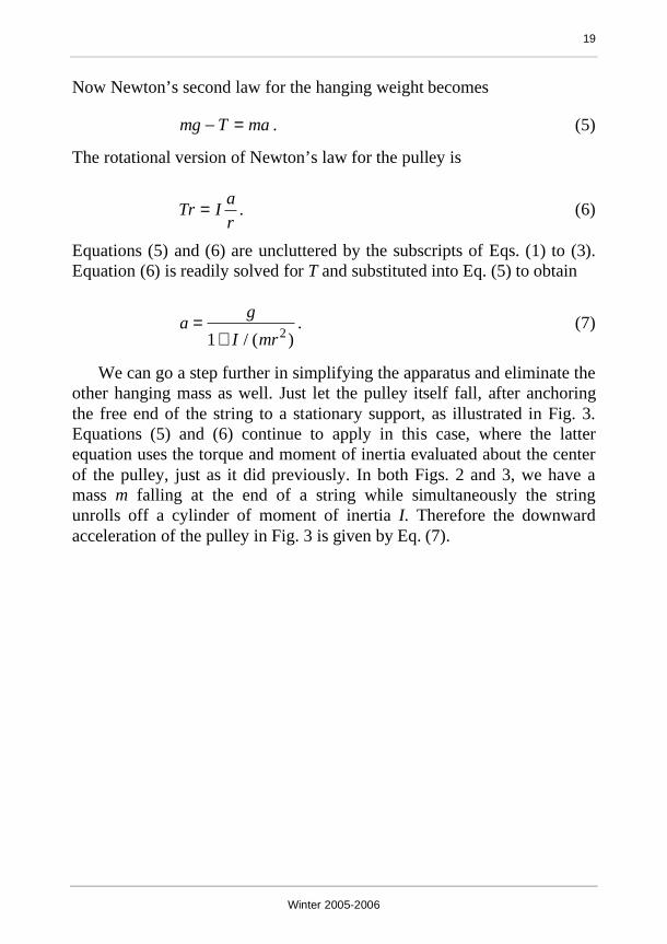
Now Newton’s second law for the hanging weight becomes

mg T = ma . (5)

The rotational version of Newton’s law for the pulley is

Tr = I

a

r. (6)

Equations (5) and (6) are uncluttered by the subscripts of Eqs. (1) to (3). Equation (6) is readily solved for T and substituted into Eq. (5) to obtain

a =g

1+ I / (mr2 )

. (7)

We can go a step further in simplifying the apparatus and eliminate the other hanging mass as well. Just let the pulley itself fall, after anchoring the free end of the string to a stationary support, as illustrated in Fig. 3. Equations (5) and (6) continue to apply in this case, where the latter equation uses the torque and moment of inertia evaluated about the center of the pulley, just as it did previously. In both Figs. 2 and 3, we have a mass m falling at the end of a string while simultaneously the string unrolls off a cylinder of moment of inertia I. Therefore the downward acceleration of the pulley in Fig. 3 is given by Eq. (7).

20

Washington Academy of Sciences

Fig. 3. Free-body diagram for a cylinder unrolling without slipping along a vertical string. The top attachment point of the string can be to your finger held stationary, making it easy to carry around and perform this demonstration. As a bonus, the cylinder rewinds itself back up after it has reached its bottom-most point.

One now has a simple apparatus to transport and demonstrate. However, it has one small flaw as drawn, in that one cannot reduce the acceleration as much as one might really like for quantitative measurements. Even if we increase the moment of inertia of the cylinder to its maximum value (for a given mass and radius) of I = mr

2 , corresponding to a hollow ring, we will only have “decreased g” by 50% when we solve for the acceleration in Eq. (7). Fortunately it is not hard to alter the device to overcome this difficulty: Use a yoyo (cf. Fig. 4) to move mass outward to a larger radius R and thus to increase I. The radius r around which the string is wrapped is not changed however, and therefore Eq. (7) remains valid.

21

Winter 2005-2006

Fig. 4. Modifying the shape of the dropped cylinder in Fig. 3 so that its moment of inertia can be increased without changing the radius r about which the string is wound.

I suggest constructing yoyos for such use as follows. Start with an identical pair of uniform disks with combined mass m, so that

I =

1

2mR

2 . Next construct the inner cylinder with radius r = R / where > 1 is the desired ratio of the outer to the inner radius of the yoyo. Use a light-weight cylinder for this purpose (a short piece of plastic pipe works well) so that its moment of inertia is negligible compared to that of the two disks. Substituting these values of I and r into Eq. (7) results in a downward translational acceleration of the yoyo of

a =g

1+2 / 2

. (8)

To make the acceleration small, choose >> 1, in which case the factor of unity can be neglected in the denominator of Eq. (8). If the yoyo is wound up on a string of length L (plus the straight dashed length in Fig. 4 so that the free end can be accessed at the rim) and released from rest, then the time T required for it to descend to the end of the string is found from a standard equation of kinematics,

22

Washington Academy of Sciences

L =

1

2aT

2 . (9)

In particular, for a 1-m drop, we therefore predict T / 3 s . For example, if = 30 , a fall time of about 10 seconds is expected, a round value one can even estimate without a timer (by counting “1001, 1002, …, 1010”). I constructed such a yoyo by cutting two 15-inch-diameter wooden disks on a bandsaw and using a half-inch-diameter plastic pipe of about 1-cm length for the inner cylinder. To assemble the yoyo, I drilled clearance holes through the centers of the wooden disks and fastened everything together with a screw and nut. This permits quick disassembly for student measurement of the inner pipe diameter or reparation of a broken string. (Although I use strong nylon line, it still breaks occasionally.) I also drilled small holes through the side of the pipe to fasten the string and keep the knot from slipping around the inner cylinder. Agreement with the exact theoretical prediction is found to within a few tenths of a second, comparable to the reaction time in its measurement. Averaging repeated trials can reduce this error further.

In conclusion, a falling yoyo is a valuable theoretical and experimental problem for inclusion in introductory physics courses. As an exercise in simultaneously applying Newton’s second law in both its translational and rotational forms, it complements other such problems in the curriculum. (It is worth noting that there are several other instructive methods, as discussed in the Appendix, of analyzing the yoyo’s descent, just as there are for Atwood’s machine.) For example, it is closely analogous to a wheel rolling without slipping down an incline. Secondly, it is a more convenient handheld apparatus than the traditional Atwood’s machine, which requires well-lubricated bearings to minimize frictional effects, a sturdy stand to support the pulley, and some form of arrestor to keep the falling weights from violently crashing into the tabletop and pulley. Thirdly, one can experimentally determine g with high accuracy merely by measuring the ratio of the outer and inner radii, the length of the string wound onto the yoyo, and the time of fall. In contrast, the standard apparatus necessitates a nontrivial measurement of the moment of inertia of the pulley.

23

Winter 2005-2006

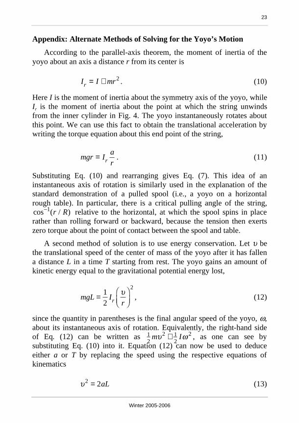
Appendix: Alternate Methods of Solving for the Yoyo’s Motion

According to the parallel-axis theorem, the moment of inertia of the yoyo about an axis a distance r from its center is

Ir

= I + mr2 . (10)

Here I is the moment of inertia about the symmetry axis of the yoyo, while Ir is the moment of inertia about the point at which the string unwinds from the inner cylinder in Fig. 4. The yoyo instantaneously rotates about this point. We can use this fact to obtain the translational acceleration by writing the torque equation about this end point of the string,

mgr = I

r

a

r. (11)

Substituting Eq. (10) and rearranging gives Eq. (7). This idea of an instantaneous axis of rotation is similarly used in the explanation of the standard demonstration of a pulled spool (i.e., a yoyo on a horizontal rough table). In particular, there is a critical pulling angle of the string,

cos 1(r / R) relative to the horizontal, at which the spool spins in place rather than rolling forward or backward, because the tension then exerts zero torque about the point of contact between the spool and table.

A second method of solution is to use energy conservation. Let be the translational speed of the center of mass of the yoyo after it has fallen a distance L in a time T starting from rest. The yoyo gains an amount of kinetic energy equal to the gravitational potential energy lost,

mgL =1

2Ir r

2

, (12)

since the quantity in parentheses is the final angular speed of the yoyo, , about its instantaneous axis of rotation. Equivalently, the right-hand side of Eq. (12) can be written as

1

2m

2+

1

2I

2 , as one can see by substituting Eq. (10) into it. Equation (12) can now be used to deduce either a or T by replacing the speed using the respective equations of kinematics

2

= 2aL (13)

24

Washington Academy of Sciences

or

2

=ave

=L

T (14)

where the middle term in Eq. (14) is the average translational speed of the yoyo over the distance L.

Finally, in an intermediate mechanics course, the acceleration of the yoyo can be instructively derived using either the Lagrangian or the Hamiltonian formalism. Consider the former for instance. There is only one generalized coordinate, which we can take to be y, the distance downward that the center of the yoyo has moved from its starting position (which position we can also take as the zero level for the gravitational potential energy); the angle of rotation of the yoyo relative to its starting orientation is constrained by the string’s no-slip condition to be = y / r . Noting that

(where the dot denotes a time derivative), the

Lagrangian (equal to the difference between the kinetic and potential energies) can be written as

L( y, y) =1

2Ir

y

r

2

+ mgy . (15)

Then Lagrange’s equation immediately gives the acceleration,

L

y=

d

dt

L

ymg =

Ir

r2

a , (16)

in agreement with Eq. (11).