A TWO-DIMENSIONAL NUMERICAL SIMULATION OF PLASMA WAKE

STRUCTURE AROUND A CUBESAT

by

Rajendra Mitharwal

A thesis submitted in partial fulfillmentof the requirements for the degree

of

MASTER OF SCIENCE

in

Electrical Engineering

Approved:

Dr. Reyhan Baktur Dr. Charles M. SwensonMajor Professor Committee Member

Dr. Bedri A. Cetiner Dr. Mark R. McLellanCommittee Member Vice President for Research and

Dean of the School of Graduate Studies

UTAH STATE UNIVERSITYLogan, Utah

2011

ii

Copyright c© Rajendra Mitharwal 2011

All Rights Reserved

iii

Abstract

A Two-Dimensional Numerical Simulation of Plasma Wake Structure Around a CubeSat

by

Rajendra Mitharwal, Master of Science

Utah State University, 2011

Major Professor: Dr. Reyhan BakturDepartment: Electrical and Computer Engineering

A numerical model was developed to understand the time evolution of a wake structure

around a CubeSat moving in a plasma with transonic speed. A cubeSat operates in the

F2 layer of ionosphere with an altitude of 300 − 600 Km. The average plasma density

varies between 10−6cm−3 − 10−9cm−3 and the temperature of ions and electrons is found

between 0.1−0.2 eV. The study of a wake structure can provide insights for its effects on the

measurements obtained from space instruments. The CubeSat is modeled to have a metal

surface, which is a realistic assumption, with a negative electric potential. To solve the

equations of plasma, the numerical difference equations were obtained by discretizing the

fluid equations of the plasma along with nonlinear Poisson’s equation. The electrons were

assumed to follow the Boltzmann’s relation and the dynamics of ions was followed using

the fluid equations. The initial and boundary conditions for the evolution of the structure

are discussed. The computation was compared to the analytical solution for a 1D problem

before being applied to the 2D model. There was a good agreement between the numerical

and analytical solution. In the 2D simulation, we observe the formation of plasma wake

structure around the CubeSat. The plasma wake structure consists of rarefaction region

where ion density and ion velocity decreases compared to the initial density and velocity.

(47 pages)

iv

I dedicate this to my brother, Virender Mitharwal.

v

Acknowledgments

I express my gratitude towards my major professor, Dr. Reyhan Baktur, for provid-

ing the opportunity to work on a topic which interests me and also providing the support

throughout my master’s program. This thesis is possible because of her knowledge, guid-

ance, feedback, and review.

I would like to thank Dr. Charles Swenson for guiding me throughout this work,

especially when the project seemed far from being possible. His knowledge in both plasma

physics and computational science had a tremendous effect on the way I completed this work.

I would also like to thank Dr. Bedri Cetiner for his guidance and support. His knowledge in

the field of microwaves has always inspired me as a researcher. I would like to acknowledge

Dr. Edmund Spencer for his inspiration. His teachings on space physics, fluid dynamics,

and partial differential equations led me to develop the necessary theoretical background in

the least possible time. I would also like to thank my graduate student advisor, Mary Lee

Anderson, for proofreading this thesis and her help throughout the graduate work.

I love and respect my parents for giving me full support and having faith in me. It’s my

dad who has instilled in me the importance of mathematics. I express my love for Kabbu

for having full faith, trust, and being the source of both inspiration and encouragement.

Rajendra Mitharwal

vi

Contents

Page

Abstract . . . . . . . . . . . . . . . . . . . . . . . . . . . . . . . . . . . . . . . . . . . . . . . . . . . . . . . iii

Acknowledgments . . . . . . . . . . . . . . . . . . . . . . . . . . . . . . . . . . . . . . . . . . . . . . . v

List of Figures . . . . . . . . . . . . . . . . . . . . . . . . . . . . . . . . . . . . . . . . . . . . . . . . . . vii

1 Introduction . . . . . . . . . . . . . . . . . . . . . . . . . . . . . . . . . . . . . . . . . . . . . . . . . 1

1.1 CubeSat Environment . . . . . . . . . . . . . . . . . . . . . . . . . . . . . . 31.2 Plasma . . . . . . . . . . . . . . . . . . . . . . . . . . . . . . . . . . . . . . . 41.3 Analytical Approach . . . . . . . . . . . . . . . . . . . . . . . . . . . . . . . 71.4 Numerical Approach . . . . . . . . . . . . . . . . . . . . . . . . . . . . . . . 81.5 Thesis Outline . . . . . . . . . . . . . . . . . . . . . . . . . . . . . . . . . . 9

2 1D Study and Results . . . . . . . . . . . . . . . . . . . . . . . . . . . . . . . . . . . . . . . . . . 11

2.1 Numerical Scheme . . . . . . . . . . . . . . . . . . . . . . . . . . . . . . . . 122.2 Simulation Parameters . . . . . . . . . . . . . . . . . . . . . . . . . . . . . . 152.3 Results . . . . . . . . . . . . . . . . . . . . . . . . . . . . . . . . . . . . . . . 16

3 2D Study and Results . . . . . . . . . . . . . . . . . . . . . . . . . . . . . . . . . . . . . . . . . . 22

3.1 Numerical Scheme . . . . . . . . . . . . . . . . . . . . . . . . . . . . . . . . 233.2 Simulation Parameters . . . . . . . . . . . . . . . . . . . . . . . . . . . . . . 263.3 Results . . . . . . . . . . . . . . . . . . . . . . . . . . . . . . . . . . . . . . . 28

4 Conclusion . . . . . . . . . . . . . . . . . . . . . . . . . . . . . . . . . . . . . . . . . . . . . . . . . . . 36

References . . . . . . . . . . . . . . . . . . . . . . . . . . . . . . . . . . . . . . . . . . . . . . . . . . . . . . 38

vii

List of Figures

Figure Page

1.1 CubeSat. . . . . . . . . . . . . . . . . . . . . . . . . . . . . . . . . . . . . . 2

2.1 Numerical scheme for fluid equations in 1D. . . . . . . . . . . . . . . . . . . 13

2.2 Numerical scheme for Poisson’s equation in 1D. . . . . . . . . . . . . . . . . 15

2.3 Plasma sheath. . . . . . . . . . . . . . . . . . . . . . . . . . . . . . . . . . . 18

2.4 Normalised ion density in 1D. . . . . . . . . . . . . . . . . . . . . . . . . . . 18

2.5 Electric potential (Volts) in 1D. . . . . . . . . . . . . . . . . . . . . . . . . . 19

2.6 Normalised ion velocity in 1D. . . . . . . . . . . . . . . . . . . . . . . . . . 19

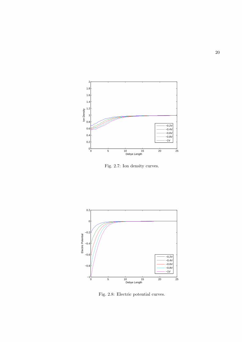
2.7 Ion density curves. . . . . . . . . . . . . . . . . . . . . . . . . . . . . . . . . 20

2.8 Electric potential curves. . . . . . . . . . . . . . . . . . . . . . . . . . . . . . 20

2.9 Velocity curves. . . . . . . . . . . . . . . . . . . . . . . . . . . . . . . . . . . 21

3.1 Numerical scheme for fluid equation Step 1. . . . . . . . . . . . . . . . . . . 24

3.2 Numerical scheme for fluid equation Step 2. . . . . . . . . . . . . . . . . . . 25

3.3 Numerical scheme for fluid equation Step 3. . . . . . . . . . . . . . . . . . . 25

3.4 Numerical scheme for Poisson’s equation in 2D. . . . . . . . . . . . . . . . . 27

3.5 Normalised density for ions entering parallel to x-axis. . . . . . . . . . . . . 30

3.6 Normalised density for ions entering at 45 degrees to x-axis. . . . . . . . . . 30

3.7 Electric potential (Volts) for ions entering parallel to x-axis. . . . . . . . . . 31

3.8 Electric potential (Volts) for ions entering at 45 degrees to x-axis. . . . . . . 31

3.9 Normalized flux along x-axis for ions entering parallel to x-axis. . . . . . . . 32

3.10 Normalized flux along x-axis for ions entering at 45 degrees to x-axis. . . . 32

3.11 Normalized flux along x-axis for ions entering parallel to x-axis. . . . . . . . 33

viii

3.12 Normalized flux along x-axis for ions entering at 45 degrees to x-axis. . . . 33

3.13 Magnitude of normalized velocity for ions entering parallel to x-axis. . . . . 34

3.14 Magnitude of normalized velocity for ions entering at 45 degrees to x-axis. . 34

3.15 Velocity vectors for ions entering parallel to x-axis. . . . . . . . . . . . . . . 35

3.16 Velocity vectors for ions entering at 45 degrees to x-axis. . . . . . . . . . . . 35

1

Chapter 1

Introduction

The concept of CubeSat began as a collaboration between academic universities to

build a deeper understanding of space without big budgets for space missions. A one unit

(1U) CubeSat is a small satellite, with a dimension of 10cm x 10cm x 10cm as shown in

Fig. 1.1 [1] and weight generally does not exceed 1Kg. The use of standardization in the

deployment programs defines the size requirement of a CubeSat [1]. In particular, the use

of Poly-Picosatellite Orbital Deployer or the P-PODs [2] which are used in the launch and

deployment of CubeSats. The P-POD has a size of three 1U CubeSats. It can accommodate

CubeSats of 1U, 1.5U, 2U, and 3U size specifications. The other specifications which affect

the design of CubeSats are the size of commercial-off-the-shelf (COTS) components (solar

cell and battery), launch vehicle environmental and operational requirement and the safety

standards [3].

The development process of CubeSats consists of requirement planning, design analysis,

fabrication, quality control, system level testing, integration, launch, and ground-based

satellite operations. The standardization across these processes is core to the features of

CubeSat Program. It helps in reducing both the mission cost and the development time.

The usual time required for the development and deployment is two years. This has caused

a growing interest of the student community in the CubeSat programs. CubeSats give

the students an opportunity to learn multi-disciplines, which in turn has made the space

technology more accessible to academia [3].

There has been varied interest in launching the CubeSat. The most common of them

is the enhancement of technology in terms of costs. This includes COTS components,

sensors, solar array and antennas [4], tethered systems, and wireless systems. The Earth

imaging is an example where these interests has enhanced the technology, particularly the

2

Fig. 1.1: CubeSat.

CMOS camera technology and altitude determination algorithms. These objectives should

help in improving our knowledge base of the science involved in space. This includes the

understanding of the environment in space and how it affects the Earth (there have been

missions to understand earthquakes). The CubeSats orbit in the F2-layer of ionosphere

at a speed of 7500 − 7800 m/s. The characteristics of the plasma found in this region is

explained in the next section.

There have been many instances where CubeSats have failed to achieve the science

objectives [5]. This necessitates that the steps during design and analysis should be carried

with more time on validation and testing. The failure rate can be reduced if there are

more testing tools available. Since the CubeSat has to work in space and its difficult to

have the same environment conditions on Earth, the computer simulation is the way to

learn the working of CubeSat. These simulations have their own advantages with respect

to cost and risks. Our work has been in this direction about how the space environment

around a CubeSat behaves which can be a valuable data for instrumentation engineers

during the design phase. Our simulation aims at understanding the dynamics in formation

of wake structure around a CubeSat, when it is placed in the orbit. This understanding

becomes important when we want to know whether the spacecraft instruments on board

are measuring the plasma properties or the disturbance created by the spacecraft itself. So,

the ultimate scientific goal behind our work with these simulations is the validation of the

3

measurements obtained from the spacecraft instruments.

In our study, we solve the problem in both 1D and 2D. In 1D case, the CubeSat is

modeled to be an infinite long metal sheet placed at the origin. In 2D case, the CubeSat

is modeled with a 2D square region moving at transonic speed and placed inside the com-

putational domain filled with plasma. The 1D case describes the basic phenomenon of the

formation of plasma sheath over an infinite metal surface. The sheath is formed because

of the high mobility of the electrons due to which they are easily diffused into the metal

wall compared to the ions. The ions accumulate around the metal surface to shield the

effect produced by the negative electric potential. The potential varies continuously from

the electric potential applied on metal surface to the plasma potential in the region. The

simulation starts with the zero initial velocity but achieves the minimum ion velocity re-

quired at pre-sheath region [6]. Plasma fluid equations are used to track the ion dynamics,

where as Boltzmann’s relation is used for electrons. In our work, we use the collisionless, un-

magnetized, and nonlinear model of the ideal plasma (two species of the charged particles)

described by fluid equations for the isothermal ions and electrons. For 1D case, there are

analytical solutions available [7] with which we compare our results. The simulation is run

longer enough to achieve the steady state where there is no change in the wake structure.

1.1 CubeSat Environment

A CubeSat operates in the F2 layer of ionosphere with the altitude range in 300-600

Km which is also known as Low Earth Orbits (LEO). They also operate at the range of

200 Km, where the wake structure becomes more important because of the presence of

the neutral atoms. These neutral atoms are not absorbed by the satellite surface and this

causes an increase in the neutral density on the front surface. The space environment at

that altitude is very complex and dynamic. The local satellite environment mainly consists

of plasma which is explained in next section. The presence of plasma in this region causes

the most common effect known as spacecraft charging. This effect is being seen in the case

of the spacecraft instruments, especially Langmuir probes, and is one of the reasons to study

the wake structure [8]. It is caused due to the electron influx causing an electric potential

4

to develop on the satellite. Sometimes the electron flux can cause damage to the circuitry

and the electronic systems. The charging of satellite is also caused due to the presence of

current flow from the plasma and occasionally due to the emission of photoelectrons from

the surface. There are many ways by which spacecraft charging can be reduced. Shielding

being one of them, or maintain the spacecraft ground at the plasma potential to stop the

flow of current. The newest method to reduce the charging effects is ejection of electron

beam out of the spacecraft. There are various effects that take place in this region [9] which

are solar ultraviolet (UV) radiation, ionizing radiation, atomic oxygen, and pressure related

effects due to presence of high vacuum. They cause mostly the surface degradation of the

material used on the CubeSats. In F2 layer, the ionization maximum takes place causing

a balance between plasma transport and chemical ion processes. The species of ions found

in this region is O+. The ion density varies from 10−6cm−3 − 10−9cm−3 [10]. The ion and

electron temperature varies from 0.1-0.2 eV [11]. For our simulation, we use 0.1 eV for both

electron and ion temperature.

1.2 Plasma

Plasma is a collection of ions, electrons, and neutral atoms formed due to process of

ionization. It differs from the ionized gas in the sense that if we consider a small volume,

small enough that there is no variation of plasma properties, and big enough that it has

large number of particles in it, it shows collective behavior [7]. The charge neutrality is

one such collective behavior. Due to its collective nature, plasma can be explained with the

help of fluid transport equations explained later in this section. Any plasma is described

using Debye length and plasma frequency. The Debye length λd is given by

λd =

(

ǫ0KT

n0e2

)

, (1.1)

where T is the temperature of the charge particles and n0 is the ambient charge particle

density of a neutral plasma. The λd determines the distance where the charge imbalance can

penetrate for a given disturbance. It also defines the shielding length, the distance where

5

impact of the external electric field can be observed. In our simulation, when a conducting

metal surface is place in the plasma, the so called charge imbalance, also known as plasma

sheath, is formed around it and its thickness is of the order of λd. The angular frequency

also known as plasma frequency is given by

ωp =

(

n0e2

meǫ0

)

, (1.2)

where me is the mass of the electron. This defines the tendency of the plasma to oscillate

due to a disturbance. The disturbance in our case was the electric field. In the presence

of this electric field, the electrons, due to their light mass compared to ions, show excellent

mobility and react immediately to the electric field where the ions remain static. This

causes a charge separation causing polarization within the plasma. The polarization gives

rise to internal electric field which tries to restore the charge neutrality. The electrons,

because of the initial kinetic energy, gained move beyond their equilibrium position and

the restoring force acts in the opposite direction of their motion and tries to bring them

back to original position. The restoring force and electron motion causes what is known

as plasma oscillations. In our simulation, we use λd and 1/ωp to normalize the space and

time, respectively.

As explained, the plasma consists of electrons, ions, and neutral particles. Therefore,

the system of fluid transport equation which describes the plasma properties is written sepa-

rately for each particle. These equations are obtained by taking moments of the Boltzmann’s

equation. The first two moments represent the density and momentum. These equations

are expressed in conservative form. The non-conservative form of expressing these equations

was used by Ward et al. [8]. The first moment is given by the following equation

∂nk

∂t+∇ · (nk~uk) = 0. (1.3)

This is known as continuity equation describing the conservation of mass. The significance

of each term can be explained by considering a small volume. First term represents the time

6

rate of change of the density of a particular species in a volume. Second term represents

the difference between outflow and inflow flux of the particles inside the small volume. The

second moment of the Boltzmann’s equation gives rise to the momentum equation given by

∂nk~uk∂t

+∇ · (nk~uk~uk) = −∇Pk

mk+

nk

mk

~F . (1.4)

On the left-hand side, the first term represents the time rate of change of a particle flux

inside a small volume, and the second term represents the difference between outflow and

inflow momentum flux of the particles. The first term on the right-hand side represents the

force experienced due to pressure, and the last term represents any general force acting on

the particles. The symbol nk represents the density, ~uk represents the velocity, mk is the

mass, and Pk is the pressure of the kth species, respectively. ~F is the Lorentz force given by

~F = e( ~E + ~uk × ~B), where e is the charge of the ion or electron, ~E represents the electric

field, and ~B is the magnetic field applied to the plasma. This is known as dyadic notation

and is expanded below for a Cartesian coordinate system.

~uk~uk = u2kxxx+ ukxukyxy + ukxukzxz

+ukyukxyx+ u2kyyy + ukyukz yz

+ukzukxzx+ ukzuky zy + u2kz zz (1.5)

So, the second term on the right-hand side of (1.4) can be written as

∇ · (nk~uk~uk) =∂

∂x

(

nku2kx + nkukyukx + nkukzukx

)

x

+∂

∂y

(

nkukxuky + nku2ky + nkukzuky

)

y

+∂

∂z

(

nkukxukz + nkukyukz + nku2kz

)

z. (1.6)

The electrostatic potential φ in the plasma sheath region is governed by Poisson’s equation

given by

∇2φ =e

ǫ0(ni − ne), (1.7)

7

where ni is the density of ions and ne is the density of electrons. Equations (1.3), (1.4),

and (1.7) together describe the evolution of plasma sheath in a space with respect to time.

The formation of sheath around a metal surface is the basic phenomenon observed

in plasma [6]. The metal surface develops the negative potential with respect to plasma

potential due to the absorption of the electrons. The ion and electron density is different in

the sheath region. The potential in the sheath region increases from the negative potential

on the metal surface to the plasma potential as we move from wall to the region where

charge neutrality is maintained. This is simulated numerically in the case of 1D problem.

1.3 Analytical Approach

The analytical approach requires some assumptions so that the fluid equations de-

scribed in previous section can be solved to provide an understanding of the plasma sheath.

The equations can be solved in 1D, but becomes more difficult to solve in higher dimension

where there are no closed forms of the solution. Since (1.4) is a nonlinear equation due to

the presence of convective term, the solution to these equations cannot be solved analyti-

cally for plasma sheath without assuming the steady state. In steady state, the first term

representing the time variation of the density or momentum is dropped. The analytical

results can be summarized in the form of following equation [7]:

ne = n0 exp

(

eφ

kTe

)

, (1.8)

where ne is the electron density and Te is the electron temperature in K. To obtain this,

we solve the momentum equation for electrons and assume the electrons to be of zero mass

compared to ions. The other assumptions which we make for the analytical solution to be

valid are Ti = Te = T and meu2e ≤ KbT ≤ miu

2i . We assume this relationship holds for the

density of the electrons to find the numerical solution of the Poisson’s equation. The ion

density is given by

ni = n0 exp

(

1−2eφ

miu0i

)− 1

2

, (1.9)

8

where mi is the mass of ion and u0i represents the ion velocity at the boundary where the

charge neutrality is maintained. The expression for this velocity is given by

u0i =

(

kTi

2πme

)1/2

exp

(

eφ0

kTe

)

, (1.10)

where φ0 is the electric potential applied to the metal surface. The electric potential in the

sheath region is given by

φ = φ0 exp

(

−x

χ

)

, (1.11)

where χ being

χ = λ2d

(

1−KTi

miu20i

)−2

. (1.12)

1.4 Numerical Approach

Since the formation of plasma sheath over a metal surface is governed by nonlinear

behavior, it is difficult to solve it analytically for unsteady and higher-dimensional (more

than one) cases. The numerical schemes can provide a great insight about the formation

of sheath, describing both transient and steady state behavior. The different numerical ap-

proach depending upon the physics can be classified into either kinetic approach or the fluid

approach. The kinetic approach requires the kinetic theory of gases, where the individual

charge particle dynamics is followed inside a volume. This requires solving the Vlasov’s

equation [12] to get the distribution function which can then be used to find the velocity

and spatial orientation of an individual charge particle. This approach is also known as

Particle In Cell (PIC) simulation.

In the fluid approach, the collective behavior of the collection of particles is used and

the plasma is treated using the fluid equations of continuity and momentum. This gives the

density and velocity behavior of the particles as a collection. PIC simulations are generally

used where wave particle interactions are of interest since fluid approach cannot by its own

nature describe the single particle dynamics. Our simulation uses fluid approach because

the ion density in the CubeSat’s environment is high and tracking single particle dynamics

9

will require large computational resources.

The computational methods are effective to understand the physical phenomenons

which are described by nonlinear partial differential equations, and the fluid transport

equation to describe the plasma behavior is one of them. These methods are not an al-

ternative to analytical or experimental way of understanding the physics, but a substitute.

As a general approach, the problem of solving a physical system numerically consists of

following steps [12].

• Define the partial differential equations describing the physical system.

• Discretize the equation, i.e. transforming the continuous models to difference equa-

tions so that they can be solved on a digital computer.

• Solve the difference equations thus obtained by defining the solution domain both

in space and time. This also involves defining a grid over both space and time. If

the solution of the difference equation depends only on the solution of previously

calculated values it is known as explicit. If the solution also depends on the future

values, then a system of linear algebraic equations are obtained and the method is

known as implicit. The solution thus obtained is an approximate one.

The different approaches to solve these equations are finite-domain time differences and

finite volume methods. In our approach, the finite volume method was used to solve for

the evolution of sheath which is similar to that used by Chavelier et al. [13]. This approach

differs from Ward et al. [8] where the nonlinear fluid equations were linearized in first order

and the non-conservative form of fluid equations was used. Both approaches simulate the

plasma fluid with initial drift velocity being zero, where as it is transonic in our 2D case.

1.5 Thesis Outline

Following the introduction, Chapter 2 defines the problem in 1D and explains the

method to achieve numerical discretization. The chapter also discusses the necessary sim-

ulation parameters. The results obtained after running the simulation to steady state are

10

summarized using plots and compared with the analytical expressions. Chapter 3 also fol-

lows the same outline as that of Chapter 2. At the end of the chapter, the results are

summarized using 2D plots. The conclusion of overall work and the future direction is

discussed in Chapter 4.

11

Chapter 2

1D Study and Results

The plasma fluid equations given by (1.3) and (1.4) are reduced to 1D and are nor-

malized both in space and time. The problem was solved in 1D to validate the numerical

model against the known analytical expressions given in section 1.3. As explained in de-

tail in the next section, the normalized equations are then discretized using the high order

nonoscillatory central schemes. The Poisson’s equation (1.7) was discretized using three

node approximation and was solved nonlinearly using the conjugate gradient schemes. The

difference equations obtained after discretization were coded into MATLABTM using the

specified initial and boundary conditions on variables of interest (density, flux, and electric

potential), and the simulation was run till the steady state was achieved and there was no

variation in the variables. The simulation results showed a good match when compared

with the analytical expressions.

The equation of continuity is given by

∂ni

∂t+

∂niui∂x

= 0. (2.1)

The equation of momentum equation given by

∂niui∂t

+∂niu

2i

∂x= −

1

mi

∂Pi

∂x+

ni

miF, (2.2)

where Pi is the pressure which is given by niKbT . Since, we are considering only the

electrostatic case. F is given by eE where E is the electric field given by−e∂φ∂x . The electric

field is calculated from the nonlinear Poisson’s equation using Boltzmann’s relationship for

12

electrons. The equation is shown below:

∂2φ

∂x2=

e

ǫ0(ni − n0 exp

(

eφ

kTe

)

). (2.3)

The equations were normalized in space and time with λd and 1/ωp, respectively. The

density was normalized with the ambient ion density n0 and the ion velocity with ion

acoustic velocity given by√

KbTi

mi. The equations are then discretized both in space and

time. Here the procedure to discretize the equations (2.1) and (2.2) would be described

using central schemes and results would be compared with analytical expressions given in

previous chapter.

2.1 Numerical Scheme

The fluid equations can be represented in the form of the following hyperbolic equation:

∂u

∂t+

∂f(u)

∂x=

∂q(u)

∂x. (2.4)

In case of equation (2.1), we have u = ni, f(u) = niui, and q(u) = 0 . Similarly for

equation (2.2) we have u = niui, f(u) = niu2i +

1mi

Pi, and q(u) = −eφ. The numerical

solution is found by defining a uniform spatial and temporal grid where time is discretized

using t = n∆t where n = (0, 1, 2 . . .), x = n∆x, and Unj = U(j∆x, n∆t). The fluid

equations were discretized using the high-resolution central schemes [14] based on finite

volume approach. The steps required to solve these equations using numerical difference

equations are explained using the computational molecule shown in Fig. 2.1 in which the

quantities used are defined by following equations:

Hj+1/2(t) =F (u+j+1/2) + F (u−j+1/2)

2

−aj+1/2

2(u+j+1/2 − u−j+1/2), (2.5)

Pj+1/2(t) =Q(uj) +Q(uj+1)

2, (2.6)

13

Fig. 2.1: Numerical scheme for fluid equations in 1D.

where aj+1/2 is the local speed in each cell. The quantities are given by

u±j+1/2 = uj+1 ∓∆x

2(ux)j+1/2∓1/2, (2.7)

where ux is given by

(ux)nj = minmod

(

unj − un−1j

∆x,un+1j − unj∆x

)

, (2.8)

and minmod limiter is defined as minmod(a, b) = 12 [sgn(a) + sgn(b)].min(|a| , |b|). The final

difference equations are defined using the following equation:

dujdt

= −Hj+1/2 −Hj−1/2

∆x

+Pj+1/2 − Pj−1/2

∆x. (2.9)

14

The Euler scheme is used to the march this equation forward in time. The time step ∆t

varies according to the Courant Friedrichs Lewy (CFL) condition given by

∆t = C/max(aj+1/2

∆x

)

, (2.10)

where C is the Courant number and is set to 1/8 in our simulations.

The equation (2.3) has a nonlinear term due to presence of Boltzmann’s relation for

electron density. The computational scheme for the same is shown in Fig. 2.2. It can be

represented in the form of the function of φ given by

h(φ) =φi+1 − 2φi + φi−1

∆x2+

e

ǫ0(ni − n0 exp

(

eφ

kTe

)

). (2.11)

This equation is solved iteratively, where φk represents the value in the kth iteration. So for

the next iteration, the φk+1 can be found using the Taylor series expansion and neglecting

the higher order terms

h(φk+1) = h(φk) + h′(φk)(φk+1 − φk) = 0, (2.12)

δk = (φk+1 − φk), (2.13)

which reduces to

h′(φk)δk = h(φk), (2.14)

which is in the form of linear system of algebraic equations AX = B. The A is found by

Jacobian matrix given by

Amn =

1/∆x2 m = i, n = i± 1

− 2∆x2 − n0e2

kTeǫexp

(

e(φ−φ0)kTe

)

m = n = i.

(2.15)

In each iteration, a linear system of equations is to be solved to obtain the value for δk.

15

Fig. 2.2: Numerical scheme for Poisson’s equation in 1D.

This value is then added to φk to obtain new value for φ at each spatial node, which is then

used in next iteration. Since the A matrix is sparse, the biconjugate gradient scheme [15]

is used to solve the linear system of equations. For each iteration, the tolerance level for

RMS error is set to 10−7. This method seems to converge if the initial guess is sufficiently

close to the solution.

2.2 Simulation Parameters

The length, density, velocity, and time were normalized using electron Debye length,

average ion density, acoustic speed of the ions and plasma period (calculated from plasma

frequency), respectively. The simulation parameters for other quantities are summarized

as:

Density n0: 1,

Electron temperature: 0.1 eV,

Ion temperature: 0.1 eV,

Plasma potential: 0 V,

Potential applied at the metal surface: −0.2 V.

The electric potential was chosen to be −0.2 V because of two reasons. First, when a

negative voltage is applied to the metal surface a stable plasma sheath is formed. Secondly,

to compare the results for analytical expressions of the ion density and electric potential

the potential on the metal wall should be comparable to the electron temperature. The

computational domain was of length L = 50λd. The small space step ∆x was chosen to be

0.2. The infinite metal wall was place at the left boundary and the inflow of the particles

was at the right boundary. The model of the system was made to evolve with the time.

16

The initial conditions were

ni(x, 0) = 1;uix(x, 0) = 0. (2.16)

The boundary conditions for the domain were

ni(L, t) = 1; φ(0, t) = −0.2; φ(L, t) = 0. (2.17)

The ui at the boundary cell were calculated using the extrapolation depending upon the

two neighboring cells.

2.3 Results

The simulation was run using MATLABTM on Windows Environment using Dual Core

AMD Opteron Processor 165 (1.81GHz). The RAM memory required for the simulation

domain was 50MB. The obtained results for ion density and electron potential were com-

pared with the analytical expressions given in section 1.3. The time taken for one plasma

period to complete was 5 seconds. The results of the 1D problem obtained after running

the simulation for 3500 plasma periods are summarized in Fig. 2.3 to Fig. 2.9. During the

initial stage, when the sheath was forming there were waves observed travelling from the

sheath region to the inflow boundary. The amplitude of these waves eventually subsides

when the steady state is achieved.

Figure 2.3 shows the final ion density and electron density. The ion density was obtained

by solving the plasma fluid equations numerically. The electric potential obtained from

Poisson’s equation was substituted in the Boltzmann’s relationship for electrons to get the

electron density. As can be seen, the result shows the formation of plasma sheath for the

applied negative electric potential. The ions and electrons arrange themselves around the

metal wall in order to create an electric field which opposes the electric field due to the

metal wall. The metal wall surface due to its negative electric potential tends to absorb

the ions and cause a slump in the ion density. Now electrons with ions are forced towards

the metal surface to maintain the charge neutrality of plasma, but because of the higher

17

mobility are removed from the region at a faster rate than the ions. This causes more

decrease in the electron density as compared to the ion density. The plasma sheath thus

formed has a thickness of 8 λd. The electrons start decreasing from the equilibrium ion

density at around 8 λd and the ions start at 5 λd.

The comparison of ion density for the simulation and analytical approach is done in

Fig. 2.4. The ion density matches perfectly in the region where the charge neutrality is

maintained. In the sheath region there is slight decrease in the ion density for simulated

results. This decrease is due to the assumptions which were made in deriving the analytical

expression for the density. In the analytical approach, the ions were assumed to be cold so

the pressure was not taken into account. In numerical approach, the pressure contributed

to the diffusion of the ions towards the metal wall.

In Fig. 2.5, we have compared the electric potential. The electric potential is equal to

the plasma potential in the nonsheath region and in the sheath region it begins to drop to

the value of the applied potential the metal surface. The electric potential shows a good

match compared to the ion density for the simulated results. This is because we are using

the difference of the ion and electron density on a small space interval for calculating the

electric potential, of which the electron density uses the analytical expression.

The simulation started with the ions having zero velocity. When the steady state is

achieved, the sheath formed, in Fig. 2.6 we see the ion velocity to be at Bohm’s Velocity

at inflow boundary and gradually increase in the sheath region to the value of 1.46 times

the thermal velocity at the metal surface. The negative value of the ions here is due to the

ions moving in negative direction. The plots showed a similar results what was observed in

the work of Chavelier et al. [13] and confirmed the validity of the scheme to simulate the

time evolution of plasma sheath over a metal surface.

Figure 2.7 to Fig. 2.9 show the simulation for the variation as we keep on increasing the

negative electric potential on the metal surface of the CubeSat. The variation of ion density

with electric potential is shown in Fig. 2.7. Figure 2.8 shows the variation of corresponding

electric potentials. As we see in Fig. 2.9, the ions are removed at faster rate when the

18

applied negative potential is increased and therefore the slump in the ion density in Fig.

2.7 increases.

As can be seen from Fig. 2.4 and Fig. 2.5, the numerical results showed a good

and reasonable agreement with the analytical expressions. This validates our numerical

approach and the same is applied to the 2D case.

0 10 20 30 40 500

0.2

0.4

0.6

0.8

1

1.2

1.4

1.6

1.8

2

Den

sity

Debye length

IonsElectrons

Fig. 2.3: Plasma sheath.

0 10 20 30 40 500

0.2

0.4

0.6

0.8

1

1.2

1.4

1.6

1.8

2

Ion

Den

sity

Debye length

SimulationAnalytical

Fig. 2.4: Normalised ion density in 1D.

19

0 10 20 30 40 50−0.2

−0.15

−0.1

−0.05

0

0.05

0.1

0.15

0.2

Debye length

Pot

entia

l

SimulationAnalytical

Fig. 2.5: Electric potential (Volts) in 1D.

0 10 20 30 40 50−2

−1.8

−1.6

−1.4

−1.2

−1

−0.8

−0.6

−0.4

−0.2

0

Vel

ocity

Debye length

Fig. 2.6: Normalised ion velocity in 1D.

20

0 5 10 15 20 250

0.2

0.4

0.6

0.8

1

1.2

1.4

1.6

1.8

2

Debye Length

Ion

Den

sity

−0.2V−0.4V−0.6V−0.8V−1V

Fig. 2.7: Ion density curves.

0 5 10 15 20 25−1

−0.8

−0.6

−0.4

−0.2

0

0.2

Debye Length

Ele

ctric

Pot

entia

l

−0.2V−0.4V−0.6V−0.8V−1V

Fig. 2.8: Electric potential curves.

21

0 5 10 15 20 25−2

−1.8

−1.6

−1.4

−1.2

−1

−0.8

−0.6

−0.4

−0.2

0

Debye Length

Ion

Vel

ocity

−0.2V−0.4V−0.6V−0.8V−1V

Fig. 2.9: Velocity curves.

22

Chapter 3

2D Study and Results

In 2D, we extend the problem which was done in 1D. The difference here is adding one

extra dimension introduces one more term for flux in the fluid equations. The objective here

is to study the dynamics of plasma around the CubeSat model. The variation of plasma

quantities is considered along x and y direction. The momentum equation representing

the motion of the ions is defined for both the directions. The process of extending to 2D

follows from the 2D fluid equations and the Poisson’s equation derived from the previously

defined equations (1.3), (1.4), and (1.7). Then we discretize these using the same schemes

which we used in 1D and validity of which was proved in the obtained simulation results.

After discretizing, the numerical difference equations were simulated using a given set of

parameters for two different directions of ion flux. The simulation was run long enough to

achieve the steady state showing the time evolution of wake structure around the CubeSat.

If we consider the evolution of the sheath in 2D, i.e. the variation of the quantities in

the x and y direction, then the equation for continuity is

∂ni

∂t+

∂(niuix)

∂x+

∂(nkuiy)

∂y= 0. (3.1)

Accordingly, the equation of momentum reduces to

∂niuix∂t

+∂(niu

2ix)

∂x+

∂(niuixuiy)

∂y= −

1

mi

∂Pi

∂x+

ni

miFx, (3.2)

∂niuiy∂t

+∂(niuixuiy)

∂x+

∂(niu2iy)

∂y= −

1

mi

∂Pi

∂y+

ni

miFy, (3.3)

where Fx = −e∂φ∂x +uiyBx and Fy = −e∂φ∂y +uixBy is the force due to electrostatic field and

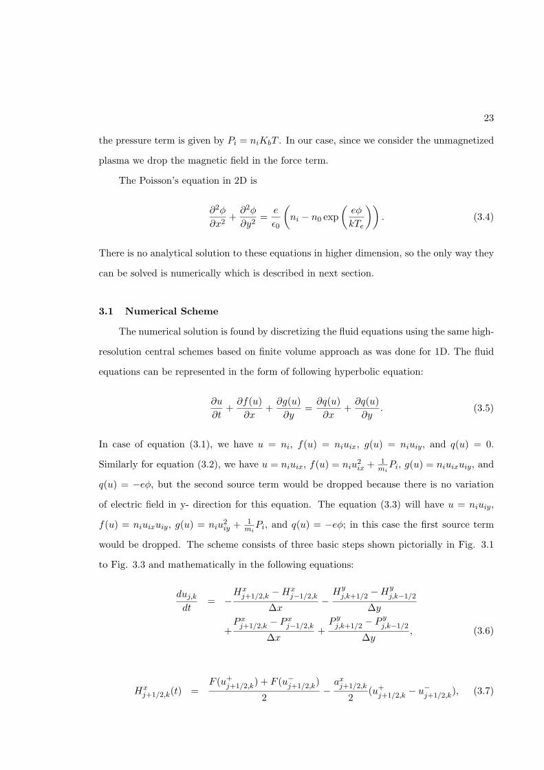
23

the pressure term is given by Pi = niKbT . In our case, since we consider the unmagnetized

plasma we drop the magnetic field in the force term.

The Poisson’s equation in 2D is

∂2φ

∂x2+

∂2φ

∂y2=

e

ǫ0

(

ni − n0 exp

(

eφ

kTe

))

. (3.4)

There is no analytical solution to these equations in higher dimension, so the only way they

can be solved is numerically which is described in next section.

3.1 Numerical Scheme

The numerical solution is found by discretizing the fluid equations using the same high-

resolution central schemes based on finite volume approach as was done for 1D. The fluid

equations can be represented in the form of following hyperbolic equation:

∂u

∂t+

∂f(u)

∂x+

∂g(u)

∂y=

∂q(u)

∂x+

∂q(u)

∂y. (3.5)

In case of equation (3.1), we have u = ni, f(u) = niuix, g(u) = niuiy, and q(u) = 0.

Similarly for equation (3.2), we have u = niuix, f(u) = niu2ix +

1mi

Pi, g(u) = niuixuiy, and

q(u) = −eφ, but the second source term would be dropped because there is no variation

of electric field in y- direction for this equation. The equation (3.3) will have u = niuiy,

f(u) = niuixuiy, g(u) = niu2iy +

1mi

Pi, and q(u) = −eφ; in this case the first source term

would be dropped. The scheme consists of three basic steps shown pictorially in Fig. 3.1

to Fig. 3.3 and mathematically in the following equations:

duj,kdt

= −Hx

j+1/2,k −Hxj−1/2,k

∆x−

Hyj,k+1/2 −Hy

j,k−1/2

∆y

+P xj+1/2,k − P x

j−1/2,k

∆x+

P yj,k+1/2 − P y

j,k−1/2

∆y, (3.6)

Hxj+1/2,k(t) =

F (u+j+1/2,k) + F (u−j+1/2,k)

2−

axj+1/2,k

2(u+j+1/2,k − u−j+1/2,k), (3.7)

24

Fig. 3.1: Numerical scheme for fluid equation Step 1.

Hyj,k+1/2(t) =

G(u+j,k+1/2) +G(u−j,k+1/2)

2−

ayj,k+1/2

2(u+j,k+1/2 − u−j,k+1/2), (3.8)

P xj+1/2,k(t) =

Q(uj,k) +Q(uj+1,k)

2, (3.9)

P yj,k+1/2(t) =

Q(uj,k) +Q(uj,k+1)

2, (3.10)

where axj+1/2,k and ayj,k+1/2 are the local speed in x and y directions, respectively, for each

cell. The quantities are given by

u±j+1/2,k = uj+1,k ∓∆x

2(ux)j+1/2∓1/2,k, (3.11)

u±j,k+1/2 = uj,k+1 ∓∆y

2(uy)j,k+1/2∓1/2. (3.12)

25

Fig. 3.2: Numerical scheme for fluid equation Step 2.

Fig. 3.3: Numerical scheme for fluid equation Step 3.

26

The Euler scheme is used to march the equation (3.6) forward in time. The time step varies

according to the CFL condition given by

∆t = C/max

(

axj+1/2,k

∆x

ayj,k+1/2

∆y

)

, (3.13)

where C is set to 1/8 for the simulation.

Equation (3.4) can be represented in the form of the function of φ given by

h(φ) =φi+1,j − 2φi,j + φi−1,j

∆x2+

φi,j+1 − 2φi,j + φi,j−1

∆y2

+e

ǫ0

(

ni − n0 exp

(

eφ

kTe

))

, (3.14)

where ne is replaced with the expression for Boltzmann’s relation for electrons given by

equation (1.8).

As given in the 1D case, the form of linear system of algebraic equations AX = B. The

computational molecule for the same is given in Fig. 3.4. Now if we have Nx grid points

along x-axis and Ny along y-axis, we get i = 1 to Nx and j = 1 to Ny. Let us define the

current node for calculating the sparse matrix as Nc = i+ (j − 1)Nx. Matrix A is found by

Jacobian matrix h′(φk) given by

Amn =

1/∆x2 m = i, n = Nc ± 1

1/∆y2 m = i, n = Nc ±Nx

− 2∆x2 − 2

∆y2− n0e

kTeǫexp

(

φ−φ0

kTe

)

m = n = Nc.

(3.15)

The tolerance level for the RMS error was decided as 10−7.

3.2 Simulation Parameters

The simulation parameters were same as that in the 1D case. The only difference here

is the computational domain has an extra dimension. The solution domain for the difference

27

Fig. 3.4: Numerical scheme for Poisson’s equation in 2D.

equation was confined along the x-axis and y-axis over a region of an area Lx × Ly. Since

the boundary for the solution of the plasma fluid equations (3.1), (3.2), (3.3), and (3.4)

exists at infinity, to solve the difference equations (3.6) and (3.14) the boundary needs to be

at some finite value. In the case of ion flux entering the domain at an angle of 45 degrees,

the boundary was chosen to be at Lx = Ly = 100λd. The number of grid points per λ was

chosen to be 2. So, the value for ∆x is 0.5λd. The metal cube of width 5 λd was placed at

(25,25) from the origin of the computational domain. For the second case where the ion flux

is parallel to x-axis, the x and y-boundary were at Lx = 70λd and Ly = 150λd, respectively.

The metal cube was placed at (25,75). The value for Lx and Ly were chosen such that

they were sufficiently large compared to the size of the metal cube, and sufficiently small

compared to the use of the collisionless plasma model. Since Boltzmann’s relationship for

the electron density was used, the mass of the ions was that of the realistic model. The

temperature of ions was equal to that of electrons. The density and velocity at inflow

boundaries were fixed on the initial values, whereas at outflow boundaries of the metal

28

surface and the computational domain were calculated using the first order extrapolation

using the interior cells. The electric potential was specified on the metal surface and was

extrapolated on the boundaries of computational domain using the linear extrapolation.

The initial condition for the case where the ion flux is 45 degrees to x-axis is given by

ni(x, y, 0) = 1; uix(x, y, 0) = 1.77; uiy(x, y, 0) = 1.77, (3.16)

and for the case where it is parallel to x-axis is

ni(x, y, 0) = 1; uix(x, y, 0) = 2.5; uiy(x, y, 0) = 0. (3.17)

3.3 Results

The RAM memory required for the simulation domain 450MB. The time taken for

one plasma period to complete was 3.5 hours. The simulation was run for 299.51 plasma

periods. The density profile showed no change after 50 plasma periods, so compared to 1D

simulation the steady state was achieved sooner. The simulation for the case where ion flux

was parallel to x-axis took more time steps for a single plasma period because of the CFL

condition requirement.

The density profile starts with single tail in the rarefaction region which divides into

two. The profile shows symmetric behavior around the ion flux direction. The wake struc-

ture expands both in the direction perpendicular and parallel to the ion flux direction.

After running the simulation for 299.51 plasma periods, we obtain the initial density profile

shown in Fig. 3.5 and Fig. 3.6 where we see the rarefaction waves at the front and back

of the metal cube. In this region, the ion density varies from 0.56 to 0.8. There was a

small density build up near the CubeSat’s rear end. This was because as we move from

the CubeSat’s rear surface towards the outflow boundary we experience the ions reversing

there direction of momentum.

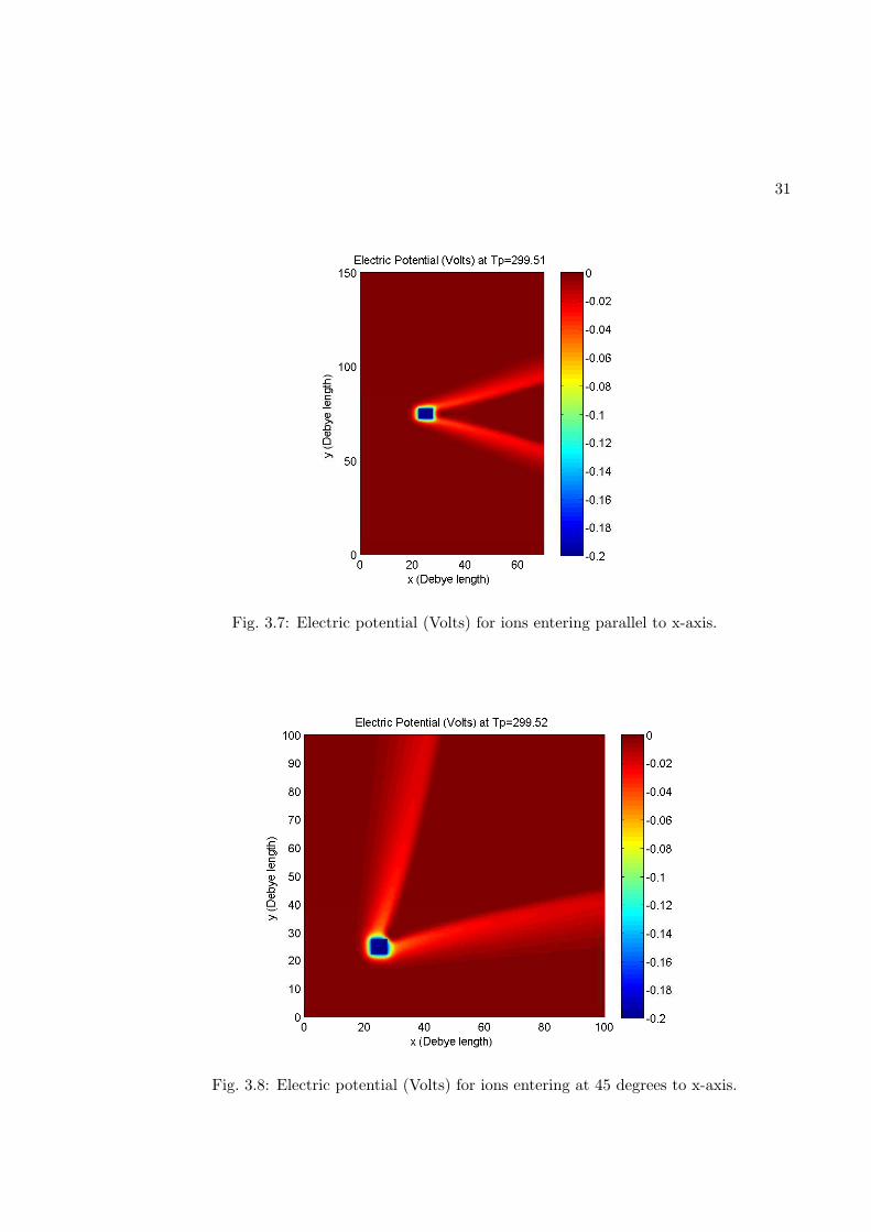
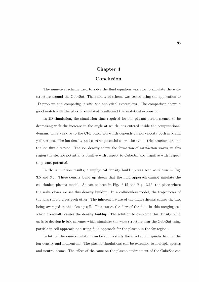
Figure 3.7 and Fig. 3.8 shows the electric potential profile. The electric potential

because of nonlinear Poisson’s equation mimics the behavior of the ion density. The electric

29

potential in the rarefaction region was found to be varying between −0.001 to −0.04V

approximately for both the case. The region behind the CubeSat was showing an electric

potential of −2× 10−4V and −8× 10−4V for the first case and second case, respectively.

The ion flux in along the x-axis is shown in Fig. 3.9 and Fig. 3.10, and along y-axis

is shown in Fig. 3.11 and Fig. 3.12. For the first case, the ion flux along x axis, we see

that the ions in the rarefaction region develop the velocity which varies from 0.2 to 0.4

magnitude where as for ion flux along y-axis shows a symmetric structure varies from 1.2

to 2. For the second case, we see the ion flux along y-axis and x-axis seems to mirror the

structure along the direction of ion flux. The value of the flux tends to reduce behind the

CubeSat for both the axis.

The magnitude of the velocity of ions is shown in Fig. 3.13 and Fig. 3.14. As can

be seen, in the rarefaction region we see the magnitude has increased than the initial ion

velocity and has decreased in the region behind the Cubesat. In the density build up region,

we see that the magnitude of the ion velocity decreases significantly compared to the other

regions of the wake structure. Figure 3.15 and Fig. 3.16 show the vector diagram for the

trajectory of ions near the CubeSat Surface. Here the ions reverse their direction of motion.

Using the plasma fluid equations, the results shows that there is formation of plasma wake

structure around the CubeSat and the ion density and the motion is affected because of the

applied electric potential.

30

Fig. 3.5: Normalised density for ions entering parallel to x-axis.

Fig. 3.6: Normalised density for ions entering at 45 degrees to x-axis.

31

Fig. 3.7: Electric potential (Volts) for ions entering parallel to x-axis.

Fig. 3.8: Electric potential (Volts) for ions entering at 45 degrees to x-axis.

32

Fig. 3.9: Normalized flux along x-axis for ions entering parallel to x-axis.

Fig. 3.10: Normalized flux along x-axis for ions entering at 45 degrees to x-axis.

33

Fig. 3.11: Normalized flux along x-axis for ions entering parallel to x-axis.

Fig. 3.12: Normalized flux along x-axis for ions entering at 45 degrees to x-axis.

34

Fig. 3.13: Magnitude of normalized velocity for ions entering parallel to x-axis.

Fig. 3.14: Magnitude of normalized velocity for ions entering at 45 degrees to x-axis.

35

23 24 25 26 27 28 29 30 31

71

72

73

74

75

76

77

78

79

Velocity Vectors at Tp=299.51

y (D

ebye

leng

th)

x (Debye length)

Fig. 3.15: Velocity vectors for ions entering parallel to x-axis.

23 24 25 26 27 28 29 30 31 32

23

24

25

26

27

28

29

30

31

32

Velocity Vectors at Tp=299.52

y (D

ebye

leng

th)

x (Debye length)

Fig. 3.16: Velocity vectors for ions entering at 45 degrees to x-axis.

36

Chapter 4

Conclusion

The numerical scheme used to solve the fluid equation was able to simulate the wake

structure around the CubeSat. The validity of scheme was tested using the application to

1D problem and comparing it with the analytical expressions. The comparison shows a

good match with the plots of simulated results and the analytical expression.

In 2D simulation, the simulation time required for one plasma period seemed to be

decreasing with the increase in the angle at which ions entered inside the computational

domain. This was due to the CFL condition which depends on ion velocity both in x and

y directions. The ion density and electric potential shows the symmetric structure around

the ion flux direction. The ion density shows the formation of rarefaction waves, in this

region the electric potential is positive with respect to CubeSat and negative with respect

to plasma potential.

In the simulation results, a unphysical density build up was seen as shown in Fig.

3.5 and 3.6. These density build up shows that the fluid apporach cannot simulate the

collisionless plasma model. As can be seen in Fig. 3.15 and Fig. 3.16, the place where

the wake closes we see this density buildup. In a collisionless model, the trajectories of

the ions should cross each other. The inherent nature of the fluid schemes causes the flux

being averaged in this closing cell. This causes the flow of the fluid in this merging cell

which eventually causes the density buildup. The solution to overcome this density build

up is to develop hybrid schemes which simulates the wake structure near the CubeSat using

particle-in-cell approach and using fluid approach for the plasma in the far region.

In future, the same simulation can be run to study the effect of a magnetic field on the

ion density and momentum. The plasma simulations can be extended to multiple species

and neutral atoms. The effect of the same on the plasma environment of the CubeSat can

37

be studied. The scheme can be extended to complex 3D environment to simulate the real

scenarios using time varying electric and magnetic fields.

38

References

[1] R. Munakata, “Cubesat design specification rev. 12,” The CubeSat Program, CaliforniaPolytechnic State University, 2009.

[2] J. Brown, “Test pod user’s guide,” The CubeSat Program, California Polytechnic StateUniversity, 2000.

[3] A. Toorian, E. Blundell, J. Puig-Suari, and R. Twiggs, “Cubesats as responsive satel-lites,” in Space Conference, American Institute of Aeronautics and Astronautics, Aug.2005.

[4] M. N. Mahmoud, “Integrated solar panel antennas for cube satellites,” Master’s thesis,Utah State University, Logan, UT, 2010.

[5] A. Toorian, K. Diaz, and S. L. , “The cubesat approach to space access,” in Aerospace

Conference, 2008 IEEE, pp. 1–14, Mar. 2008.

[6] K. U. Riemann, “Residual vector quantizers with jointly optimized code books,” Jour-

nal of Physics, vol. 24, pp. 493–518, 1991.

[7] J. A. Bittencourt, Fundamentals of Plasma Physics. New York: Springer, 2004.

[8] J. Ward, C. Swenson, and C. Furse, “The impedance of a short dipole antenna in amagnetized plasma via a finite difference time domain model,” Antennas and Propa-

gation, IEEE Transactions on, vol. 53, no. 8, pp. 2711–2718, Aug. 2005.

[9] E. Grossman and I. Gouzman, “Space environment effects on polymers in low earthorbit,” Nuclear Instruments and Methods in Physics Research Section B: Beam Inter-

actions with Materials and Atoms, vol. 208, pp. 48–57, 2003.

[10] R. A. Heelis, “Electrodynamics in the low and middle latitude ionosphere: a tutorial,”Journal of Atmospheric and Solar-Terrestrial Physics, vol. 66, no. 10, pp. 852–838,2004.

[11] P. M. Banks, “Thermal conduction and ion temperatures in the ionosphere,” Earth

and Planetary Science Letters, vol. 1, no. 5, pp. 270–275, 1966.

[12] E. Halickova, “Fluid model of plasma and computational methods for solution,” inWeek of Doctoral Students 06 Proceedings of Contributed Papers: Part III, pp. 180–186, 2006.

[13] T. W. Chavelier, U. S. Inan, and T. F. Bell, “Fluid simulation of the collisionlessplasma sheath surrounding an electric dipole antenna in the inner magnetosphere,”Radio Science, vol. 45, RS1010, p. 18, 2010.

[14] A. Kurgnov and E. Tadmor, “New high-resolution central schemes for nonlinear con-servation laws and convection-diffusion equations,” Journal of Computational Physics,pp. 241–246, 2000.

39

[15] R. J. Leveque, Finite Difference Methods for Ordinary and Partial Differential Equa-

tions: Steady-State and Time-Dependent Problems. Philadelphia: SIAM, 2007.