attribute-based clustering for information dissemination...
TRANSCRIPT

Attribute-Based Clustering for InformationDissemination in Wireless Sensor Networks1
Ke Wang, Salma Abu Ayyash, Thomas D.C. Little
Department of Electrical and Computer Engineering
Boston University, Boston, Massachusetts 02215, USA
(617) 353-9877
{ke,saayyash,tdcl}@bu.edu
Prithwish Basu
BBN Technologies
10 Moulton St, Cambridge, Massachusetts 02138, USA
MCL Technical Report No. 07-13-2005
Abstract– Data routing in large wireless sensor networks is challenged by requirements
for scalability, robustness, and energy use, as well as the possibility that globally unique
identifiers for each node are nonexistent. Moreover, if the sensor network serves multiple
functions or users, its routing function must be energy efficient when responding to information
requests (inquiries) that can arrive at high rates, require diverse data types, and target
subsets of the sensor network.
We propose virtual “containment” hierarchies based on relevant attributes as a more
efficient mechanism to disseminate inquiries rather than the use of flooding schemes. We
show algorithms that support clustering sensors according to these hierarchies and implement
clusterhead failure recovery and load balancing among cluster members. We show that our
framework has significant bandwidth gains over a flooding-based scheme under the scenario
considered using analytical techniques.
1Proc. 2nd Annual IEEE Communications Society Conf. on Sensor and Ad Hoc Communications andNetworks (SECON 2005), Santa Clara, CA, Sept. 2005. This work is supported by the NSF under grantNo. CNS-0435353. Any opinions, findings, and conclusions or recommendations expressed in this materialare those of the author(s) and do not necessarily reflect the views of the National Science Foundation.

1 Introduction
The use of electronic sensors with wireless communication capacity to monitor environmental
phenomena is increasing [1, 2, 3]. In most of these systems there is rarely a need for
device addressing beyond a small locality (e.g., temperature of a region or location of a
tracked object). However, with the decreasing cost of wireless sensor network devices and
the increasing number of sensing capabilities that a single device can exhibit, a deployed
sensor network has resources that can fulfill many functions and overlaid missions. For
example, a single mote can sense light, relative humidity, temperature, pressure and has a
two-axis accelerometer [4]. Increasingly this sensing capability is moving to handle the larger
complexity of audio and video data [5].
We envision these many-functioned capabilities of the sensor nodes not strictly as a
baseline for building specific sensing applications but rather as serving multiple, overlaid
missions involving possibly distinct tasks. One could imagine these missions as co-located or
collaborative, potentially performing integration of data originating from different locations
or functions of the sensor network. An example of this kind of integration might be the
correlation of habitat weather data with the tracking of animals.
Characteristic of this setting is the sometimes independent, sometimes dependent collection,
dissemination, and consumption of data originating from diverse sensor devices in the network.
Consumers are expected to be applications, classes of users, and individual users each
with different data requirements and communication needs. Under these circumstances,
a deployed sensor network can be subject to a high inquiry arrival rate (due to being able to
collect varied sets of data that are of interest to different user communities), in which each
inquiry requests data from only a subset of the sensor nodes (reflecting different areas of
interest from the users of the sensor network). In this scenario, flooding mechanisms such as
Directed Diffusion [6] are inefficient because each inquiry can trigger a flooding to the whole
network, even when only a subset of sensors are relevant to the inquiry.
To address this issue, we propose establishing a hierarchy of attributes which form the
basis of the most common inquiries, and in which an upper level attribute contains the
attributes of a lower level. For example, the attribute “building” contains the “floor”
attribute, which in turn contains an attribute “room.” By clustering sensors according
to such an attribute hierarchy, we can forward inquiries to only the relevant parts of the
sensor network and thus save energy and reduce network traffic. In this paper we show
algorithms that can cluster the sensors according to a pre-defined attribute hierarchy, support
2

insertion and deletion of hierarchy levels, and implement clusterhead fault tolerance and load
balancing mechanisms by rotating the clusterhead functionality among cluster members.
We also demonstrate analytically that inquiry dissemination over such virtual hierarchy has
significant bandwidth gains over a flooding-based scheme under the scenario considered.
The remainder of the paper is organized as follows. In Sec. 2 we describe related work.
Our attribute hierarchy representation and our clustering algorithms are presented in Sec. 3.
In Sec. 4 we compare our hierarchical clustering scheme with a flooding scheme. We conclude
in Sec. 5.
2 Related Work
Node clustering techniques are significant for our approach and much work exists [7, 8, 9,
10, 11, 6, 12]. Lin and Gerla [7] select clusterheads based on node ID, while Ramanathan
and Steenstrup [8] propose forming clusters based on link quality. Clustering is proposed in
both cases to provide scalability and service guarantees. Admission control and bandwidth
allocation are all performed within the cluster. Amis et al. [9] propose an election algorithm
that chooses clusterheads in such a way that these form a dominating set. Moreover, nodes
are guaranteed to be at most d hops away from a clusterhead. McDonald and Znati [13]
propose to form clusters in order to offer probabilistic bounds on path availability. The path
availability model is built on top of a mobility model that is presented in the same paper.
Banerjee and Khuller [10] proposed algorithms that form and maintain a hierarchical set of
clusters under mobility. The clusters formed satisfy certain design objectives, such as nodes
belonging to a constant number of clusters at one hierarchy level, low overlap between two
clusters, etc. Ramachandran et al. [11] propose algorithms that form star shaped clusters at a
pre-defined maximum size, with the Bluetooth [14] model in mind. Estrin et al. [6] proposed
a clustering mechanism that can ensure bi-directional link connectivity for nodes in the
network. Ghiasi et al. [12] propose an optimal k-clustering algorithm for sensor networks,
in which k clusterheads are selected and the clusters are balanced. It is shown that this
problem is solved optimally using min-cost network flow.
The clustering algorithms above attempt formation of clusters that satisfy certain invariant
properties (leaders have lowest ID), communication metrics (link quality, bi-connectivity) or
topological properties (maximum cluster radius, balanced clusters, path availability, etc.).
Our algorithms form clusters that reflect possible traffic patterns. By tying attributes that
are relevant to inquiries posed to the sensor network to the overlaid cluster structure, we are
3

establishing clusters that reflect application level communication needs rather than network
level topological criteria.
Clustering algorithms that satisfy application level communication requirements have
also been proposed [15, 16, 17]. Clusterheads in LEACH (Low Energy Adaptive Clustering
Hierarchy [15]) and HEED (Hybrid Energy-Efficient Distributed Clustering [16]) are all
elected through a randomized algorithm which guarantees that the role of a clusterhead
is shared by all available nodes. HEED specifically uses residual energy in clusterhead
election. Bandyopadhyay and Coyle [17] use stochastic geometry to derive an expression
for the communication cost of cluster members to the clusterhead. From this expression
the cluster radius and the probability of a node becoming a clusterhead is obtained. Our
work differs from the above in that there is no support in their clustering algorithms (or
architectures) to exploit biased communication patterns in sensor networks, which we believe
will be evident if a large sensor network becomes a shared resource.
DataSpace [18] and SINA (Sensor Information Networking Architecture [19]) are additional
relevant schemes for sensor networks. DataSpace [18] is a generalized geography-based
(using GPS coordinates) routing architecture that can support querying and monitoring
of objects in the DataSpace. It uses hierarchical data cubes (which represent 3D regions
in space) and directory services in data cubes to achieve its goals. There is no reference to
specific clustering mechanisms in this work. Clustering and attribute-based naming are both
mentioned in SINA; however, the clustering algorithm is not tied to the attributes of sensors,
and is proposed only to facilitate scalable operations. Our scheme is distinct in its ability
to exploit traffic patterns via a hierarchy and the absence of reliance on GPS positioning
coordinates.
Because our work supports delivering queries to relevant regions of the network, this
can be seen as complementary to data-centric storage approaches, such as GHT (Geographic
Hash Tables) [20], DIMENSIONS [21], DIFS (Distributed Index of Features in Sensor networks) [22],
DIM (Distributed Index of Multi-dimensional data) [23] and Fractionally Cascaded Information
(FCI) [24]. In GHT, DIM and DIFS the emphasis is in finding ways to store data in a pre-
determined way so that queries can efficiently find the necessary information. GHT and
DIM use geographical hash functions that store data in pre-determined regions, while DIFS
distributes data to multiple sensors according to the value of the data and the pre-defined
spatial coverage each sensor has. This construction allows load balancing over index nodes
and supports range queries as well. Our approach establishes hierarchies within the network
and summaries of information so that queries may be routed to where the sensors containing
4
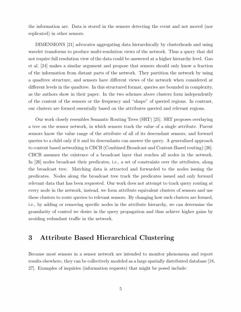
the information are. Data is stored in the sensors detecting the event and not moved (nor
replicated) in other sensors.
DIMENSIONS [21] advocates aggregating data hierarchically by clusterheads and using
wavelet transforms to produce multi-resolution views of the network. Thus a query that did
not require full resolution view of the data could be answered at a higher hierarchy level. Gao
et al. [24] makes a similar argument and propose that sensors should only know a fraction
of the information from distant parts of the network. They partition the network by using
a quadtree structure, and sensors have different views of the network when considered at
different levels in the quadtree. In this structured format, queries are bounded in complexity,
as the authors show in their paper. In the two schemes above clusters form independently
of the content of the sensors or the frequency and “shape” of queried regions. In contrast,
our clusters are formed essentially based on the attributes queried and relevant regions.
Our work closely resembles Semantic Routing Trees (SRT) [25]. SRT proposes overlaying
a tree on the sensor network, in which sensors track the value of a single attribute. Parent
sensors know the value range of the attribute of all of its descendant sensors, and forward
queries to a child only if it and its descendants can answer the query. A generalized approach
to content based networking is CBCB (Combined Broadcast and Content-Based routing) [26].
CBCB assumes the existence of a broadcast layer that reaches all nodes in the network.
In [26] nodes broadcast their predicates, i.e., a set of constraints over the attributes, along
the broadcast tree. Matching data is attracted and forwarded to the nodes issuing the
predicates. Nodes along the broadcast tree track the predicates issued and only forward
relevant data that has been requested. Our work does not attempt to track query routing at
every node in the network, instead, we form attribute equivalent clusters of sensors and use
these clusters to route queries to relevant sensors. By changing how such clusters are formed,
i.e., by adding or removing specific nodes in the attribute hierarchy, we can determine the
granularity of control we desire in the query propagation and thus achieve higher gains by
avoiding redundant traffic in the network.
3 Attribute Based Hierarchical Clustering
Because most sensors in a sensor network are intended to monitor phenomena and report
results elsewhere, they can be collectively modeled as a large spatially distributed database [18,
27]. Examples of inquiries (information requests) that might be posed include:
5

• How many nests in the northeast section of the forest currently have birds in them?
• What is the average temperature in the laboratories in the basement of building 10?
• Detect congestion in the intersection of Main and Broadway and control traffic lights
to relieve the congestion.
• What is the frequency of vibration at 12:00?
If we relied on data flooding to disseminate the inquiries within the sensor network, all
sensors would be affected whenever an inquiry requested a different type of data, which can be
energy inefficient. To save energy, we propose clustering the sensors according to attributes
that are meaningful to the inquiries and that can be exploited to reduce unnecessary traffic.
One candidate that fulfills the requirements is to establish hierarchies of attributes that
are location based, and in which upper level hierarchies contain lower level hierarchies.
By location we mean attributes that are spatially related and by containment we imply
that sensors that share a common lower level attribute automatically share all upper level
hierarchy attributes.
We choose the location attribute as the clustering criterion for several reasons: (1)
location attributes are general enough to be used in most environments (“geographical
section” clusters for sensors covering a national park, “room” clusters inside a building, etc.);
(2) hierarchies can also be easily built (room ⊂ floor ⊂ building, etc.); (3) the containment
of lower level clusters by higher level ones allows us finer control over the selection of sensors
that will receive an inquiry; and (4) it is easier to implement adaptive schemes which may go
back and forth between pure flooding schemes, which is the same as having only one cluster
containing all sensors, and hierarchically clustered schemes, depending on the dynamic cost
effectiveness analysis. The process of designing and specifying the hierarchies is beyond
the scope of this paper. We assume the existence of an attribute hierarchy, which we
interchangeably call “containment hierarchy” (CH).
In the presence of these hierarchical clusters, lower level clusterheads collect cluster
member information into “catalogs” and send them to their upper level clusterheads. When
inquiries arrive, they are processed and relayed by the top level clusterhead to the lower level
clusterheads according to the catalog information possessed. Only when the inquiries arrive
at the relevant clusters are they flooded to all the sensors in the clusters. Such location based
containment hierarchies map themselves naturally to many scenarios (buildings, geographical
areas) and can be represented as directed acyclic graphs (DAGs), as can be seen from the
examples in Fig. 1. We call such DAGs Containment-DAGs or C-DAGs for short.
6

[Country]
[Coast]
[State]
[Weather−
balloon]
[Buoy]
Temperature Pressure
[Building]
[Floor]
[Corridor] [Room] [Tree]
[Nest]
[Section]
[Forest] [Town]
[Root]
[Garden]
[House]
[Neighborhood]
[Closet]
Temperature Humidity Motion Chemical
Figure 1: Examples of Attribute Containment Hierarchies
In Fig. 1 we show three examples of containment DAGs (C-DAGs). Nodes in black
represent attributes that are relevant for users of the sensor network. White boxes represent
types of data that can be collected by deployed sensors. Thus the leftmost C-DAG can be
used to collect information regarding temperature and humidity conditions in a building,
while the rightmost C-DAG can be used for temperature and pressure sensors monitoring
weather conditions along the coast. In the center C-DAG of Fig. 1 we show an example
of two attribute hierarchies (for “Forest” and for “Town”) that have a common relevant
attribute (“Tree”). In the figure, sensors with the same room number automatically share
the same floor number. Sensors in the same garden have to be in the same neighborhood.
Our current work applies mainly to static or almost static sensor networks, as represented
by habitat [2], traffic [3] or structural integrity monitoring applications [1], and by sensor
network fields deployed for target classification and tracking [28]. It is possible to support
non-location based clusters (e.g., sensors belonging to the same “family”) by forming initially
a location-based attribute hierarchy and establishing registration and update mechanisms to
cope with physical distance and/or mobility. This is however reserved for future work. We
present next our clustering algorithm.
3.1 Attribute Based Clustering
The algorithms we developed form same-attribute clusters with one clusterhead and rotate
the clusterhead functionality among cluster members. Clusterheads will also gather information
regarding their cluster members so as to be able to decide whether to flood or drop inquiries
that reach them. Cluster sizes are constrained whenever possible, so as to avoid managing
disproportionately large clusters. Devices with higher energy levels are selected in the
clusterhead rotation process. Unicast routes are established among adjacent level clusterheads
in the process to facilitate any future information exchange. In addition the algorithms detect
and recover from clusterhead failures and support dynamic membership updates, effectively
7
allowing dynamic CH level updates (i.e., the containment relationships may adapt to the
types of inquiries). Specific parts of the algorithms are presented below.
CLUST_FORM
packet with more suitableReceives
leader information. ResendsCLUST_FORM packet.
MEMBER
CLUSTER
UNCLUSTERED
CLUSTER
LEADER
CLUST_FORMReceivespacket. Resend CLUST_FORM
if it contains more suitableleader information.
CLUST_FORMReceives
CLUST_FORM packet.leader information. Resend
packet with suitableReceives CLUST_FORM
timer.
packet with no suitableleader information or abovemaximum hop threshold. StartCandidacy
CLUST_FORM
leader information.packet with less suitableReceives
Candidacy timertime−out. Send
withCLUST_FORM
self as leader.
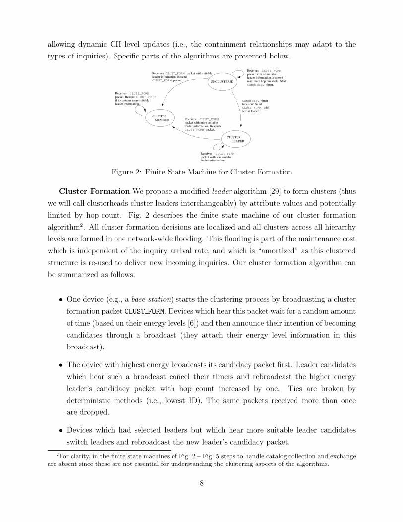
Figure 2: Finite State Machine for Cluster Formation
Cluster Formation We propose a modified leader algorithm [29] to form clusters (thus
we will call clusterheads cluster leaders interchangeably) by attribute values and potentially
limited by hop-count. Fig. 2 describes the finite state machine of our cluster formation
algorithm2. All cluster formation decisions are localized and all clusters across all hierarchy
levels are formed in one network-wide flooding. This flooding is part of the maintenance cost
which is independent of the inquiry arrival rate, and which is “amortized” as this clustered
structure is re-used to deliver new incoming inquiries. Our cluster formation algorithm can
be summarized as follows:
• One device (e.g., a base-station) starts the clustering process by broadcasting a cluster
formation packet CLUST FORM. Devices which hear this packet wait for a random amount
of time (based on their energy levels [6]) and then announce their intention of becoming
candidates through a broadcast (they attach their energy level information in this
broadcast).
• The device with highest energy broadcasts its candidacy packet first. Leader candidates
which hear such a broadcast cancel their timers and rebroadcast the higher energy
leader’s candidacy packet with hop count increased by one. Ties are broken by
deterministic methods (i.e., lowest ID). The same packets received more than once
are dropped.
• Devices which had selected leaders but which hear more suitable leader candidates
switch leaders and rebroadcast the new leader’s candidacy packet.
2For clarity, in the finite state machines of Fig. 2 – Fig. 5 steps to handle catalog collection and exchangeare absent since these are not essential for understanding the clustering aspects of the algorithms.
8

• When a device hears a cluster formation packet from a neighbor device which has a
different attribute value in one of its CH levels (e.g., sensor 23 in room 445 hears from
a sensor in room 442), it will try to become a leader candidate of the region with new
attribute value (sensor 23 becomes leader candidate for room 445).
• Devices keep track of the hop count to the leader they are selecting and the neighbor
devices through which they heard the packet. If it exceeds a pre-defined CH level
threshold value, then the device will become a leader candidate and form a new cluster
within the same attribute value region (thus room 445 may have more than one cluster).
We call this hop-count based new cluster formation.
• Cluster leaders at the lowest CH level wait for a specified time interval before flooding
(within the cluster) a request for cluster member information from its members. All
cluster leaders wait a time out period (proportional to the cluster hop-threshold number,
collect any member related information into a “catalog” and forward a summary of the
information they collected to their higher level leader. This is so that top level leaders
can make informed decisions on whether to forward or drop an arriving inquiry.
� � �� � �� �
� �� � �� � �� � �� � �� � �� � �
� �� �� �� �� �� �
� �� �� �� �� �� �� �� �
� � �� � �� � �
� �� �� �� �
� � �� � �� � �
� �� �� �� �� �� �
����
����
���� ���� ���� ����
��������
!!
""##$ $$ $% %% %
& && &''(())
**++,,--
. .. ./ // /00112 22 23 33 3
4 4 44 4 45 5
5 5
[Floor = 3]
[Floor = 1]
[Floor = 2] Floor leader
Room leader
Building leader
Sensors
Entry point for query
Floor cluster
Room cluster
[Room = 3] [Room = 4]
[Room = 2] [Room = 3] [ Room = 4 ]
[ Room = 1 ] [ Room = 2 ]
[ Room = 1 ]
BC D E
F
IJ
K L
M
PQ
R
A
H
NO
S
G
Figure 3: Attribute Containment-Based Clustering.
Note that clustering happens simultaneously across all CH levels. Thus our clustering
scheme requires only one network-wide broadcast for the formation of the clusters at all CH
levels. Although we apply node energy level as an attribute for leader selection, this is is not
intrinsic to the algorithm and is not limiting. Any function of a sensor’s attributes can be
used for leadership candidacy. The hop-count based new cluster formation rule is overridden
when there is attribute change in a lower level CH value. If there is no lower level, then new
clusters may be formed as soon as the hop-count limit is reached. This is to avoid having
different clusters in the same room answer to different floor leaders.
9

We show an example of our clustering algorithm in Fig. 3. Cluster formation starts from
node A, which elects itself as building, floor, and room leader. When it broadcasts the cluster
formation packet, node M accepts A’s building leadership, but notices that the packet came
from a different floor and room, and elects itself as leader of its floor and its room. Upon
M ’s broadcast, node O accepts M ’s floor leadership, but keeps its own room leadership
candidacy and eventually becomes room leader. Node S accepts leadership from A and M ,
canceling any candidacy timers it may have. As cluster formation packet propagates, new
room clusters are formed if the rooms are large (e.g., rooms 1 and 2 on floor 3) but since
different floor clusters cannot be formed in the same room, there is only one floor cluster
on floor 2. On floor 1, nodes G and H both broadcast their floor candidacy close to one
another, but G is the “most suitable” leader because we used the lowest id function as a tie
breaker. Node H remained room leader because of the hop distance between itself and G.
The building cluster encompassing all sensors has not been shown for sake of clarity.
Cluster Leader Rotation Leader rotation avoids single devices from being completely
energy-depleted due to their burden in the clusterhead role. The rotation period is adjusted
according to the frequency of inquiries arriving at the cluster and to the leader’s level in the
hierarchy level (higher level leaders rotate less). The steps in our algorithm are:
1. After a time-out interval, the sensor with the highest energy left in the cluster floods
the cluster announcing its leadership candidacy, establishing a routing tree rooted at
itself;
2. If multiple candidacies are heard, the “most suitable” (determined through a localized
decision) is selected;
3. The old leader, upon time-out, unicasts its catalog information to the newly elected
leader via the routing tree, and the new leader sends a catalog information update to
its higher level leader. This update establishes the unicast route from the new leader
to the higher level leader.
Fig. 4(a) shows the finite state machine of the rotation algorithm with the characteristics
listed above.
Cluster Recovery Algorithms Cluster leaders send periodic LEADER ALIVE messages
to its k-hop neighbors (k being a tunable parameter of the algorithm). These neighbors
also keep a copy of whatever information the cluster leader is maintaining. The neighbor
which detects cluster leader failure floods the cluster identifying itself as “interim leader”
10

CLUSTER
LEADER
MEMBER
CLUSTER
Send Rotation timer time−out.
Rotation.
NEW_LEADER packetwith self as leader. Restart
Receivespacket with less suitableleader information.
NEW_LEADER
Send Rotation timer time−out.
NEW_LEADER packetwith self as leader.
Receivespacket with less suitableleader information.
NEW_LEADER
Receives NEW_LEADER
with more suitable leaderinformation. ResendNEW_LEADER.
packet
NEW_LEADERReceivespacket with suitable leaderinformation. Restarttimer. Resend packet.
Rotation
MEMBER
CLUSTER
CLUSTER
LEADER
Receives LEADER_INTERIM packetwith more suitable leader information.Resend LEADER_INTERIM.
LEADER_ALIVEReceivespacket. Restart LeaderUpdate
timer.
Receives LEADER_INTERIM
packet. Resend if it contains moresuitable leader information.
LeaderAlive timer time−out.Send LEADER_ALIVE
LeaderAlive.
packet. Restart
Receives LEADER_INTERIM
packet with less suitableleader information.
Send LeaderUpdate timer time−out.
LEADER_INTERIM
packet with self as leader.
Figure 4: Finite State Machine for (a) Leader Rotation and (b) Leader LEADER ALIVE PacketExchange with k-hop Neighbors
CLUSTER_INFO packetpacket. Send suitable
if possible.
JOIN_CLUSTERReceives
threshold
JOIN_CLUSTERSends packet.times, startAfter
NewClustertimer.
Resend if it contains
more suitable leader
information.
ReceivesNEW_CLUSTER packet.
CLUSTER_INFOReceivespacket with no suitable
timer.NewCluster
maximum hop threshold. Startleader information or above
NewCluster
with self as leader.
timer time−out.Send NEW_CLUSTER packet
NEW_CLUSTER
leader informationpacket with less suitableReceives
NEW_CLUSTER
leader informationpacket with more suitableReceives
packet with suitable leaderReceives CLUSTER_INFO/NEW_CLUSTER
information.
CLUSTER
LEADER
MEMBER
CLUSTER
UNCLUSTERED
Receives JOIN_CLUSTER
packet. Send suitableCLUSTER_INFO
packet if possible.
Figure 5: Finite State Machine for joining existing clusters
(see Fig. 4(b)) and a rotation mechanism follows. Cluster member failures do not trigger
any recovery mechanisms, for we assume the sensor network to be dense enough, in which
individual sensor failures do not impair cluster related functions and properties.
If the network is not large or not dense enough, then peer monitoring among same-
attribute leaders may be necessary to recover from partitions in the attribute value region.
For example, consider the case in which a sensor in room 445 fails and breaks one cluster into
two partitions, but both are reachable through sensors along the corridor. In these instances,
the partition without a leader will detect soon that no leader rotation packets have traversed
it. After a fixed time-out value plus a random interval of time one of the sensors in the
partition will broadcast an attribute-limited cluster formation packet and a leader candidacy
packet, attempting to form a new cluster. After the new leader is established it will collect
catalog information from its members and contact its immediately higher level leader.
11

Cluster Join and CH Update Algorithms Newly deployed sensors will attempt
to join the “best” neighboring clusters that have the same attribute values. They do so by
broadcasting a request for membership packet. If no answer is received for n such broadcasts
(with exponentially increasing intervals) then the sensor remains isolated and will cluster only
when a cluster formation packet arrives. Thus all initial sensors are isolated until “triggered”
by an external signal from their base-station.
However, if there are clustered sensors nearby, they will answer the membership request
by sending their CH instance information, as well as all of their CH cluster information.
The new sensor may join the “best” cluster (at each CH level), if attributes match, or may
attempt to form a new cluster. Fig. 5 shows the finite state machine for cluster join and
update algorithms.
This mechanism effectively supports dynamic CH updates. If there is an addition of a
CH level, then sensors receiving the CH update are effectively “new without-leader” (in that
level) sensors which are in an already deployed network. They will request membership
but will receive cluster information without any matching CH level instance, at which point
they will group themselves together and elect new leaders. These new leaders will contact
(potentially through flooding the higher level cluster) their higher level leaders and lower
level leaders (if they exist) and re-establish the unicast communication architecture among
adjacent level clusterheads.
To complete our discussion of dynamic CH updates, note that the removal of a level does
not affect any member, since sensors kept all information for all CH levels. They simply
erase the information regarding that level. Leaders of the level below the removed one send
catalog update information to leaders two levels up in the old CH (such paths were formed
when the higher level leaders were elected). In the next section we present a communication
cost analysis of our hierarchical clustering mechanism and of flooding based schemes.
4 Cost Analysis of Containment Hierarchy and Flooding
Techniques
In this section we present an analysis to establish the effectiveness of creating and maintaining
CHs over the lifetime of a sensor network as compared to a flooding-based scheme. We focus
on the communication cost for the dissemination of inquiries since power consumption in a
sensor node is dominated by radio communication [25].
12

Preliminary Considerations The interaction of a community of users with a deployed
sensor network can be represented as inquiries that arrive to the sensor network with a certain
rate λ. Each arriving inquiry affects a portion Q of the sensors in the network according to
a probability distribution function PQ. The set of all possible portions Q is denoted S. We
make the following simplifications before proceeding to some theoretical analysis:
1. We assume that the cost of “tagging” the sensors so that they become aware of their
attributes is the same for both schemes;
2. The arrival rate λ represents the rate of arrival of requests for data of a type not queried
previously and/or from sensors of a different attribute, i.e., requests that trigger a
flooding in the flooding-based schemes. As stated previously, our scenario is consisted
of a network of multi-modal sensors. This network is a shared resource, and its users
are members from diverse research communities. The arrival λ models the multiple
inquiries that are initiated by this aggregate pool of users.
3. We assume that answers to inquiries traverse through paths formed during inquiry
propagation, and such paths form an inverted tree structure. The exact number of
transmissions needed to send the collected data back is dependent on the tree structure
of each scheme (CHs and flooding), and is left for future research. However, since
the underlying mechanism is the same (tree structures), we believe that the order of
magnitude of the number the transmissions in both cases is similar.
4. The cost we compute is that of the number of transmissions required to deliver the
inquiry. Although the cost of listening cannot be neglected, the analysis we perform
here is between our scheme and flooding schemes. In the absence of different scheduling
mechanisms, counting the number of transmissions yields the same estimate of power
consumption in both schemes (i.e., in both schemes the same number of sensors will
be listening at each transmission).
We will next derive some quantitative cost comparison results between CH and flooding
based schemes.
4.1 Analytical Results
Flooding Costs In a flooding based scheme, when a new inquiry arrives, it is flooded to
the whole network. In such schemes, a wireless network composed of N sensors, deployed
13

over total time epoch T , incurs the following expected cost CostF lood for inquiry delivery:
CostF lood = λ T N (1)
A scheme that actively maintains a CH structure L on top of the sensor network will have
two cost components: a maintenance cost Cost(mnt)CH and an inquiry dependent cost Cost
(inq)CH .
The maintenance cost involves communication costs needed to establish hierarchies, clusters,
message exchanges between clusterheads for coordination and catalog information dissemination
for inquiry forwarding. Note, however, that such maintenance cost is inquiry independent,
i.e., it does not increase with the frequency of new inquiries. The inquiry dependent cost
Cost(inq)CH is the cost incurred in forwarding the inquiry to only the relevant parts of the
network, based on the hierarchical structure L. In order to compare CostF lood and CostCH ,
we will study an example scenario and derive analytical expressions for CostCH and compare
it with Eq. 1.
6 6 6 6 6 6 6 6 6 6 6 6 6 66 6 6 6 6 6 6 6 6 6 6 6 6 66 6 6 6 6 6 6 6 6 6 6 6 6 66 6 6 6 6 6 6 6 6 6 6 6 6 66 6 6 6 6 6 6 6 6 6 6 6 6 66 6 6 6 6 6 6 6 6 6 6 6 6 66 6 6 6 6 6 6 6 6 6 6 6 6 66 6 6 6 6 6 6 6 6 6 6 6 6 66 6 6 6 6 6 6 6 6 6 6 6 6 66 6 6 6 6 6 6 6 6 6 6 6 6 66 6 6 6 6 6 6 6 6 6 6 6 6 66 6 6 6 6 6 6 6 6 6 6 6 6 66 6 6 6 6 6 6 6 6 6 6 6 6 66 6 6 6 6 6 6 6 6 6 6 6 6 66 6 6 6 6 6 6 6 6 6 6 6 6 66 6 6 6 6 6 6 6 6 6 6 6 6 66 6 6 6 6 6 6 6 6 6 6 6 6 66 6 6 6 6 6 6 6 6 6 6 6 6 66 6 6 6 6 6 6 6 6 6 6 6 6 66 6 6 6 6 6 6 6 6 6 6 6 6 6
7 7 7 7 7 7 7 7 7 7 7 7 7 77 7 7 7 7 7 7 7 7 7 7 7 7 77 7 7 7 7 7 7 7 7 7 7 7 7 77 7 7 7 7 7 7 7 7 7 7 7 7 77 7 7 7 7 7 7 7 7 7 7 7 7 77 7 7 7 7 7 7 7 7 7 7 7 7 77 7 7 7 7 7 7 7 7 7 7 7 7 77 7 7 7 7 7 7 7 7 7 7 7 7 77 7 7 7 7 7 7 7 7 7 7 7 7 77 7 7 7 7 7 7 7 7 7 7 7 7 77 7 7 7 7 7 7 7 7 7 7 7 7 77 7 7 7 7 7 7 7 7 7 7 7 7 77 7 7 7 7 7 7 7 7 7 7 7 7 77 7 7 7 7 7 7 7 7 7 7 7 7 77 7 7 7 7 7 7 7 7 7 7 7 7 77 7 7 7 7 7 7 7 7 7 7 7 7 77 7 7 7 7 7 7 7 7 7 7 7 7 77 7 7 7 7 7 7 7 7 7 7 7 7 77 7 7 7 7 7 7 7 7 7 7 7 7 77 7 7 7 7 7 7 7 7 7 7 7 7 7
8 8 8 8 8 8 8 88 8 8 8 8 8 8 88 8 8 8 8 8 8 88 8 8 8 8 8 8 88 8 8 8 8 8 8 88 8 8 8 8 8 8 88 8 8 8 8 8 8 88 8 8 8 8 8 8 88 8 8 8 8 8 8 88 8 8 8 8 8 8 8
9 9 9 9 9 9 9 99 9 9 9 9 9 9 99 9 9 9 9 9 9 99 9 9 9 9 9 9 99 9 9 9 9 9 9 99 9 9 9 9 9 9 99 9 9 9 9 9 9 99 9 9 9 9 9 9 99 9 9 9 9 9 9 99 9 9 9 9 9 9 9
: : : :: : : :: : : :: : : :: : : :; ; ; ;; ; ; ;; ; ; ;; ; ; ;; ; ; ;
< < << < << < << < <= = == = == = =
> > >> > >> > >> > >? ? ?? ? ?? ? ?
@ @ @@ @ @@ @ @@ @ @A A AA A AA A A
B BB BC CC CD DD DD DD DE EE EE EE E
Inquiry Forwarding
Base Station
Sensors Affected
Lake (Region of Interest)
(c) 3 Level Structure(b) 2 Level Structure(a) Flat Structure (1 Level)
Figure 6: Inquiries are propagated differently in a sensor network depending on theexistence of hierarchy levels: (a) contains one hierarchy level, (b) two hierarchy levels,and (c) three hierarchy levels.
Consider now Fig. 6. In the left-most part (Fig. 6(a)) there is only a single-level flat
network. The communication costs associated with inquiry delivery in this flat network
and flooding based schemes is equivalent. In this case there is no hierarchy maintenance
costs. However, when an inquiry for the lake arrives, even though only sensors in the lake
need respond, still the inquiry reaches all sensors in the whole square area, since there is
no mechanism to distinguish one sensor from another. In Fig. 6(b) we establish a hierarchy
with one extra upper level (two levels total) and divide the area into four quadrants. In this
case the same inquiry will affect only 1/4 of the sensors of Fig. 6(a) plus sensors involved
in forwarding the inquiry from the base station to the lower-left quadrant. In this case a
maintenance cost exists to establish and preserve the structure of quadrants (i.e., establishing
14

the clusters that map to the four quadrants, choosing clusterheads and maintaining load
balancing schemes), as well as inquiry forwarding costs. In Fig. 6(c) we add another level.
With this we reduce the number of sensors affected by the inquiry to only 1/16 of those in
Fig. 6(a) and to 1/4 of those in Fig. 6(b). The trade-off in Fig. 6(c) is a higher maintenance
cost for the two extra levels and a higher inquiry forwarding cost, if the region relevant to
the inquiry is far from the base-station.
In our example, first the inquiry is forwarded from the point of entry (e.g., a base station)
to the top level (level = 1) leader. If the inquiry is for the whole network, the latter floods
it, otherwise it forwards the inquiry to appropriate leaders at level = 2 (with appropriate
region attribute). These will likewise determine whether the inquiry is for their whole region,
in which case they flood the region, or forward the inquiry to appropriate sub-region leaders
(these will then flood their sub-region, and so on). The cost of flooding the network is N ,
while that of a region with level = 2 is N/4 and a sub-region with level = 3, N/16 etc.
Unicasts from the base station to the top level leader have estimated cost of the order of√2N since there are as many hops in the longest path in the square area. Likewise, the cost
estimate for forwarding the inquiry from a level 2 leader to a level 3 leader is of the order of√
2N2
.
Cost of Containment Hierarchy Maintenance CH scheme has an associated “maintenance
cost” for the entire epoch due to the periodic rotation of clusterheads. Suppose the clusterhead
rotation period at level = i is Ti for i = 1 to `max. The total maintenance cost is then given
by:
Cost(mnt)CH = N + 2N
`max∑
i=1
T
Ti
+√
2N`max∑
i=2
2i T
Ti
(2)
Initial clustering involves one network-wide broadcast that contributes N (first term
in Eq. 2) to the cost since each node transmits a broadcast packet only once. The rest
of the terms correspond to cluster maintenance costs. There are TTi
clusterhead rotations
at level = i. Each rotation at level = i requires one broadcast at that level followed
by all sensors in the cluster responding to update the catalog information. The broadcast
contributes N to the cost at each level and so does the catalog update step. This accounts for
the second term in Eq. 2. The third term corresponds to the unicast cost of communication
of catalogs between cluster leaders, and is a simplification of 4√
2N TT1
+ 16√
2N2
TT2
+ · · · .
Cost of Inquiry Dissemination Now, consider a model where one particular region at
level = `max receives an inquiry with probability p. For example, the region getting inquiry
in Fig. 6(b) (we will henceforth refer to this region as R). For simplicity, we assume that
15

inquiries involving the rest of the possible combinations are equiprobable with probability
q, e.g., q = 1−p
14for `max = 2. In this model, the average cost incurred for dissemination of
inquiries over time T is given by:
Cost(inq)CH = λT{
√2N +
∑
Q∈S
PQCQ} (3)
In Eq. 3 the estimated cost of forwarding an inquiry from the base station to the top
level leader is of the order of√
2N . This analysis assumes the presence of one leader per
attribute-value region. The second term expresses the cost of disseminating the inquiry
to its intended destinations while using the constructed hierarchy. The summation occurs
over all elements Q in the set S of all possible combinations of sub-regions in the sensor
network. In general there are s = 4`max−1 sub-regions and hence |S| = 2s − 1. PQ is
the probability of an inquiry involving the particular combination of sub-regions Q from
the set S and CQ is the cost of disseminating that particular style of inquiry. If Q spans
all sub-regions in the network (level = 1), then CQ = N ; if it only spans m < 4 sub-
regions at level = 2, then CQ = m(√
2N + N4). If Q involves m sub-regions r1, r2, . . . , rm
at level = 2 and also involves specific subregions inside each of these rk’s at level = 3 (say,
{r11, . . . , r1n1 ; r21, . . . , r2n2 ; · · · ; rm1, . . . , rmnm}, then the cost is given by:
CQ =m
∑
k=1
{√
2N + nk(
√2N
2+
N
16)} (4)
The CQ term for a general level i ≤ `max can be expressed similarly as a sum of costs
due to unicast and scoped broadcast within attribute sub-regions as have been illustrated
above (not presented here). For `max = 2 the total average cost incurred for dissemination
of inquiries for the epoch T is given by:
Cost(inq)CH = λT{p(
√2N +
N
4) +
3
14(1 − p)(
√2N +
N
4) +
6
14(1 − p)(2
√2N +
N
2) +
4
14(1 − p)(3
√2N +
3N
4) +
(1 − p)N +√
2N} (5)
The total communication cost corresponding to our CH-based scheme is given by:
CostCH = Cost(mnt)CH + Cost
(inq)CH (6)
16
0 0.2 0.4 0.6 0.8 10
0.1
0.2
0.3
0.4
0.5
0.6
Level 2 Rotation Period, T2 (days)
Gai
n ov
er F
lood
ing
(G)
N=10000; T=365 days; T1=5 T
2; p=0.5
λ = 64 Q/dayλ = 128 Q/dayλ = 256 Q/dayλ = 512 Q/dayλ = 1024 Q/dayλ = 2048 Q/day
0 0.2 0.4 0.6 0.8 10
0.1
0.2
0.3
0.4
0.5
0.6
Level 2 Rotation Period, T2 (days)
Gai
n ov
er F
lood
ing
(G)
N=10000; T=365 days; T1=5 T
2; p=0.067
λ = 64 Q/dayλ = 128 Q/dayλ = 256 Q/dayλ = 512 Q/dayλ = 1024 Q/dayλ = 2048 Q/day
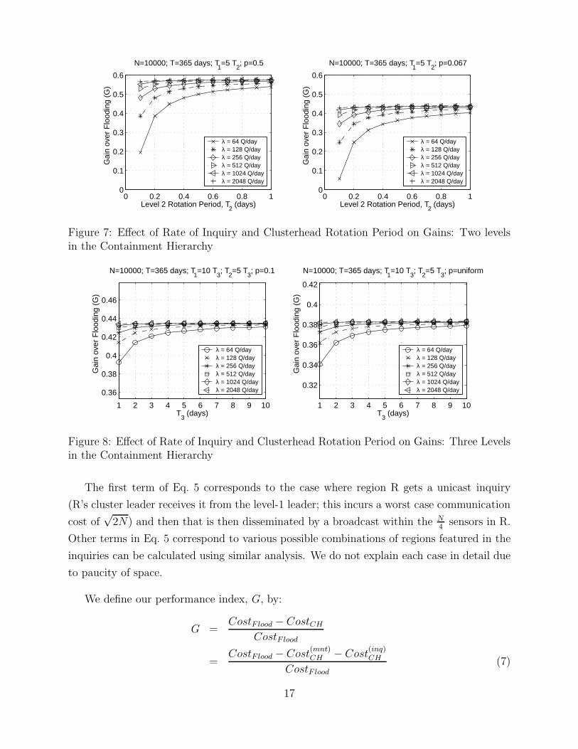
Figure 7: Effect of Rate of Inquiry and Clusterhead Rotation Period on Gains: Two levelsin the Containment Hierarchy
1 2 3 4 5 6 7 8 9 10
0.36
0.38
0.4
0.42
0.44
0.46
T3 (days)
Gai
n ov
er F
lood
ing
(G)
N=10000; T=365 days; T1=10 T
3; T
2=5 T
3; p=0.1
λ = 64 Q/dayλ = 128 Q/dayλ = 256 Q/dayλ = 512 Q/dayλ = 1024 Q/dayλ = 2048 Q/day
1 2 3 4 5 6 7 8 9 10
0.32
0.34
0.36
0.38
0.4
0.42
T3 (days)
Gai
n ov
er F
lood
ing
(G)
N=10000; T=365 days; T1=10 T
3; T
2=5 T
3; p=uniform
λ = 64 Q/dayλ = 128 Q/dayλ = 256 Q/dayλ = 512 Q/dayλ = 1024 Q/dayλ = 2048 Q/day
Figure 8: Effect of Rate of Inquiry and Clusterhead Rotation Period on Gains: Three Levelsin the Containment Hierarchy
The first term of Eq. 5 corresponds to the case where region R gets a unicast inquiry
(R’s cluster leader receives it from the level-1 leader; this incurs a worst case communication
cost of√
2N) and then that is then disseminated by a broadcast within the N4
sensors in R.
Other terms in Eq. 5 correspond to various possible combinations of regions featured in the
inquiries can be calculated using similar analysis. We do not explain each case in detail due
to paucity of space.
We define our performance index, G, by:
G =CostF lood − CostCH
CostF lood
=CostF lood − Cost
(mnt)CH − Cost
(inq)CH
CostF lood
(7)
17
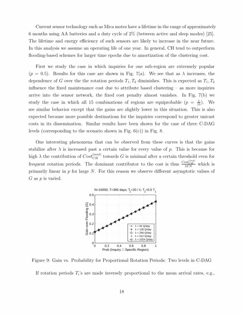
Current sensor technology such as Mica motes have a lifetime in the range of approximately
6 months using AA batteries and a duty cycle of 2% (between active and sleep modes) [25].
The lifetime and energy efficiency of such sensors are likely to increase in the near future.
In this analysis we assume an operating life of one year. In general, CH tend to outperform
flooding-based schemes for larger time epochs due to amortization of the clustering cost.
First we study the case in which inquiries for one sub-region are extremely popular
(p = 0.5). Results for this case are shown in Fig. 7(a). We see that as λ increases, the
dependence of G over the the rotation periods T1, T2 diminishes. This is expected as T1, T2
influence the fixed maintenance cost due to attribute based clustering – as more inquiries
arrive into the sensor network, the fixed cost penalty almost vanishes. In Fig. 7(b) we
study the case in which all 15 combinations of regions are equiprobable (p = 115
). We
see similar behavior except that the gains are slightly lower in this situation. This is also
expected because more possible destinations for the inquiries correspond to greater unicast
costs in its dissemination. Similar results have been shown for the case of three C-DAG
levels (corresponding to the scenario shown in Fig. 6(c)) in Fig. 8.
One interesting phenomena that can be observed from these curves is that the gains
stabilize after λ is increased past a certain value for every value of p. This is because for
high λ the contribution of Cost(mnt)CH towards G is minimal after a certain threshold even for
frequent rotation periods. The dominant contributor to the cost is thusCost
(inq)CH
λTNwhich is
primarily linear in p for large N . For this reason we observe different asymptotic values of
G as p is varied.
0 0.2 0.4 0.6 0.8 10
0.1
0.2
0.3
0.4
0.5
Prob (Inquiry ∈ Specific Region)
Gai
n ov
er F
lood
ing
(G)
N=10000; T=365 days; T1=20 / λ; T
2=0.5 T
1
λ = 64 Q/dayλ = 128 Q/dayλ = 256 Q/dayλ = 512 Q/dayλ = 1024 Q/day
Figure 9: Gain vs. Probability for Proportional Rotation Periods: Two levels in C-DAG
If rotation periods Ti’s are made inversely proportional to the mean arrival rates, e.g.,
18

Ti = ai
λ, then Eq. 7 becomes:
G = 1 − (1
λT+ 2
`max∑
i=1
1
ai
+
√
2
N
`max∑
i=2
2i
ai
) −
(
√
2
N+
1
N
∑
Q∈S
PQCQ) (8)
In this case gain G essentially becomes independent of λ and linearly increases with probability
p. This can be seen in Fig. 9.
In this section, we demonstrated that CH schemes yield gains over flooding-based schemes
when there are sub-regions in the sensor network that are more targeted than others, i.e.,
when the distribution of inquiries is not uniformly distributed over time and space. We
also showed that with increase in inquiry rate λ, CH schemes perform better since their
structures can be re-used and are more directed towards specific target regions, whereas in
a flooding-based scheme, a network-wide broadcast is necessary for each inquiry.
5 Conclusion
In this paper we showed a cost analysis of flooding based mechanisms for triggering data
collection versus mechanisms which actively maintain a hierarchical structure to deliver
inquiries. We show that under heavy utilization and high degree of sharing among a large
community, sensor networks employing pure flooding systems are expected to be less efficient
when compared to an attribute-based hierarchical system.
We propose an algorithm which is capable of supporting such hierarchies. This algorithm
is our main contribution. It enables hierarchical clustering of sensors based on common
attributes, and supports dynamic addition and removal of levels in the hierarchy. In addition,
our algorithm is fast, requiring only one network wide flooding to establish all clusters across
all hierarchy levels. It is also robust with respect to clusterhead failure, and implements load
balancing by rotating the clusterhead functionality among cluster members.
References
[1] J. Paek, N. Kothari, K. Chintalapudi, S. Rangwala, N. Xu, J. Caffrey, R. Govindan,
S. Masri, J. Wallace, and D. Whang, “The Performance of a Wireless Sensor Network
19

for Structural Health Monitoring,” in 2nd European Workshop on Wireless Sensor
Networks, Istanbul, Turkey, Jan 31 – Feb 2 2005.
[2] A. Mainwaring, D. Culler, J. Polastre, R. Szewczyk, and J. Anderson, “Wireless Sensor
Networks for Habitat Monitoring,” in Proc. 1st ACM Intl. Workshop on Wireless Sensor
Networks and Applications (WSNA’02), 2002, pp. 88–97.
[3] S. Coleri, S. Y. Cheung, and P. Varaiya, “Sensor Networks for Monitoring Traffic,” in
42nd Annual Allerton Conference on Communication, Control, and Computing, U. of
Illinois, September 2004.
[4] J. Hill and D. Culler, “MICA: A Wireless Platform For Deeply Embedded Networks,”
IEEE Micro, vol. 22, no. 6, pp. 12–24, Nov/Dec 2002.
[5] “Stargate Datasheet,” URL, http://xbow.com/Products/Product pdf files/Wireless
pdf/Stargate Datash%eet.pdf.
[6] D. Estrin, R. Govindan, J. Heidemann, and S. Kumar, “Next Century Challenges:
Scalable Coordination in Sensor Networks,” in Proc. 5th ACM MobiCom Conference,
Seattle, WA, August 1999.
[7] C. R. Lin and M. Gerla, “Adaptive Clustering for Mobile Wireless Networks,” IEEE J.
Sel. Areas in Communication (JSAC), vol. 15, no. 7, September 1997.
[8] R. Ramanathan and M. Steenstrup, “Hierarchically-Organized Multihop Mobile
Networks for Quality-of-service Support,” ACM/Baltzer J. Mobile Networks and
Applications, vol. 3, no. 2, August 1998.
[9] A. D. Amis, R. Prakash, T. Vuong, and D. Huynh, “Max-Min D-Cluster Formation in
Wireless Ad Hoc Networks,” in Proc. IEEE INFOCOM’00, Tel Aviv, March 2000.
[10] S. Banerjee and S. Khuller, “A Clustering Scheme for Hierarchical Control in Multi-
hop Wireless Networks,” in Proc. IEEE INFOCOM’01, Anchorage, Alaska, USA, April
2001.
[11] L. Ramachandran, M. Kapoor, A. Sarkar, and A. Aggarwal, “Clustering Algorithms for
Wireless Ad Hoc Networks,” in Proc. 4th Intl. workshop on Discrete Algorithms and
Methods for Mobile Computing and Communications (DIALM’00), 2000.
[12] S. Ghiasi, A. Srivastava, X. Yang, and M. Sarrafzadeh, “Optimal Energy Aware
Clustering in Sensor Networks,” SENSORS Journal, vol. 2, no. 7, pp. 258–269, July
2002.
20

[13] B. McDonald and T. F. Znati, “A Mobility-Based Framework for Adaptive Clustering
in Wireless Ad Hoc Networks,” IEEE J. Sel. Areas in Communication (JSAC), vol. 17,
no. 8, August 1999.
[14] “Bluetooth Consortium,” URL, http://www.bluetooth.com.
[15] W. Heinzelman, A. Chandrakasan, and H. Balakrishnan, “Energy-Efficient
Communication Protocols for Wireless Microsensor Networks,” in Hawaiian Intl.
Conference on Systems Science (HICSS), Hawaii, January 2000.
[16] O. Younis and S. Fahmy, “HEED: A Hybrid, Energy-Efficient, Distributed Clustering
Approach for Ad-hoc Sensor Networks,” IEEE Transactions on Mobile Computing,
vol. 3, no. 4, pp. 366–379, Oct-Dec 2004.
[17] S. Bandyopadhyay and E. Coyle, “An Energy Efficient Hierarchical Clustering
Algorithm for Wireless Sensor Networks,” in Proc. IEEE INFOCOM’03, 2003.
[18] T. Imielinski and S. Goel, “DataSpace - Querying and Monitoring Deeply Networked
Collections in Physical Space,” IEEE Personal Communications, October 2000, special
Issue on Networking the Physical World.
[19] C. C. Shen, C. Srisathapornphat, and C. Jaikaeo, “Sensor Information Networking
Architecture and Applications,” IEEE Personal Communications, pp. 52–59, August
2001.
[20] S. Ratnasamy, B. Karp, L. Yin, F. Yu, D. Estrin, R. Govindan, and S. Shenker, “GHT:
A Geographic Hash Table for Data-Centric Storage,” in Proc. 1st ACM Intl. Workshop
on Wireless Sensor Networks and Applications (WSNA’02), Atlanta, GA, September
2002.
[21] D. Ganesan, D. Estrin, and J. Heidemann, “DIMENSIONS: Why do we need a new Data
Handling architecture for Sensor Networks?” in Proc. 1st Workshop on Hot Topics In
Networks (HotNets-I), Princeton, NJ, October 2002.
[22] B. Greenstein, D. Estrin, R. Govindan, S. Ratnasamy, and S. Shenker, “DIFS: A
Distributed Index for Features in Sensor Networks,” in Proc. 1st IEEE Intl. Workshop
on Sensor Network Protocols and Applications (SNPA’03), 2003.
[23] X. Li, Y. J. Kim, R. Govindan, and W. Hong, “Multi-dimensional Range Queries
in Sensor Networks,” in Proc. 1st ACM Conference on Embedded Networked Sensor
Systems (Sensys’03), Los Angeles, CA, USA, November 2003.
21

[24] J. Gao, L. J. Guibas, J. Hershberger, and L. Zhang, “Fractionally Cascaded Information
in a Sensor Network,” in Proc. 3rd Intl. Symposium on Information Processing in Sensor
Networks (IPSN’04), 2004, pp. 311–319.
[25] S. Madden, M. Franklin, J. Hellerstein, and W. Hong, “The Design of an Acquisitional
Query Processor for Sensor Networks,” in Proc. ACM SIGMOD, San Diego, CA, June.
2003.
[26] A. Carzaniga, M. J. Rutherford, and A. L. Wolf, “A Routing Scheme for Content-Based
Networking,” in Proc. IEEE INFOCOM’04, Hong Kong, China, 2004.
[27] P. Bonnet, J. E. Gehrke, and P. Seshadri, “Querying the Physical World,” IEEE
Personal Communications, vol. 7, no. 5, pp. 10–15, October 2000, special Issue on
Smart Spaces and Environments.
[28] R. R. Brooks, P. Ramanathan, and A. M. Sayeed, “Distributed Target Classification
and Tracking in Sensor Networks,” Proc. of the IEEE, vol. 91, no. 8, August 2003.
[29] J. A. Hartigan, Clustering Algorithms. New York, NY: Wiley, 1975.
22