attitude determination and control system of a nanosatellite
TRANSCRIPT

Attitude Determination and Control System of a
Nanosatellite
by
Johannes Schoonwinkel
Thesis presented at the University of Stellenbosch inpartial fulfilment of the requirements for the degree of
Master of Science in Engineering
Department of Electrical EngineeringUniversity of Stellenbosch
Private Bag X1, 7602 Matieland, South Africa
Study leader: Prof W.H. Steyn
October 2007

Declaration
I, the undersigned, hereby declare that the work contained in this thesis is
my own original work and that I have not previously in its entirety or in part
submitted it at any university for a degree.
Signature: . . . . . . . . . . . . . . . . . . . . . . . . . . .
J. Schoonwinkel
Date: . . . . . . . . . . . . . . . . . . . . . . . . . . . . . . . .
Copyright © 2007 University of Stellenbosch
All rights reserved.

Abstract
The aim of this project was to design and test a partial attitude determina-
tion and control system for a nanosatellite. The reaction wheel system was
designed and tested as an actuator for the nanosatellite. This reaction wheel
system consists of four reaction wheels mounted in a tetrahedral formation.
A rate sensor system was also designed and its viability for this space ap-
plication was examined. The rate sensor system consists of 3 orthogonally
mounted planes, each with three rate sensors mounted on it. Hardware-in-
the-loop tests were used along with an air bearing experimentational setup,
which created near frictionless circumstances, to prove the effectiveness of
the designed reaction wheel setup. The results following from this project
were the following: The reaction wheel system proved to be an adequate ac-
tuator for this nanosatellite application and the rate sensor system which was
analysed proved to be inadequate for a nanosatellite application.
ii

Samevatting
Die doel van hierdie projek was om ’n gedeeltelike orientasie beheer stelsel
vir ’n nanosatelliet te ontwerp en te toets. Die reaksiewiel stelsel is ontwerp
en getoets as ’n aktueerder vir die nanosatelliet. Die reaksiewiel stelsel bestaan
uit vier reaksiewiele wat in ’n tetrahedrale formasie monteer is. ’n Rotasie
tempo sensor sisteem is ook ontwerp en die bruikbaarheid daarvan vir hier-
die ruimtetoepassing is ondersoek. Die rotasie tempo sensor sisteem bestaan
uit drie ortogonaal gemonteerde vlakke wat elk drie rotasie tempo sensore
bevat. Hardeware-in-die-lus toetse is saam met ’n luglaer eksperimentele
opstelling gebruik, wat semi-wrywingslose toestande skep, om die effekti-
witeit van die reaksiewiel stelsel te bewys. Die resultate wat uit hierdie pro-
jek gevolg het was die volgende: Die reaksiewiel stelsel sal as ’n baie effek-
tiewe aktueerder vir hierdie nanosatelliet toepassing gebruik kan word en
die rotasie tempo sensor stelsel wat analiseer is, is ongeskik bevind vir die
nanosatelliet toepassing.
iii

Acknowledgements
I would like to thank the following people:
• Prof Steyn for your guidance and excellent advice throughout the project
• Emile Rossouw, Izak Marais, Leo Herselman, Keith Brown, Helgard
van Rensburg, Gerrit Kruger, Henk Marais, Carlo Botha, John Wilson,
Steven Kriel, Niel Muller, Christiaan Brand and Hendrik Meiring for
your inputs and help when it was needed most
• Suné de Klerk for your wonderful support and encouragement
• My family for bringing me this far
iv
Contents
Declaration i
Abstract ii
Samevatting iii
Acknowledgements iv
Contents v
List of Figures x
List of Tables xiii
List of Abbreviations and Symbols xiv
1 Introduction 1
1.1 Aims and Objectives . . . . . . . . . . . . . . . . . . . . . . . . 1
1.1.1 Mission Objectives . . . . . . . . . . . . . . . . . . . . . 2
1.2 Background . . . . . . . . . . . . . . . . . . . . . . . . . . . . . 2
1.3 Document Layout . . . . . . . . . . . . . . . . . . . . . . . . . . 3
2 Theory 4
2.1 Space Mission Geometry . . . . . . . . . . . . . . . . . . . . . . 4
2.1.1 Coordinate Systems . . . . . . . . . . . . . . . . . . . . 4
2.1.2 Orbit parameters . . . . . . . . . . . . . . . . . . . . . . 6
2.2 Control Algorithms . . . . . . . . . . . . . . . . . . . . . . . . . 8
2.2.1 Quaternion feedback . . . . . . . . . . . . . . . . . . . . 8
2.2.2 PD control . . . . . . . . . . . . . . . . . . . . . . . . . . 9
Variable limiter attitude error feedback . . . . . . . . . 10
v

CONTENTS vi
2.3 Tetrahedral Configuration . . . . . . . . . . . . . . . . . . . . . 11
2.3.1 Conversion Matrix . . . . . . . . . . . . . . . . . . . . . 11
3 Simulation 14
3.1 Simulation Models . . . . . . . . . . . . . . . . . . . . . . . . . 15
3.1.1 Satellite Model . . . . . . . . . . . . . . . . . . . . . . . 16
3.1.2 Orbit Model . . . . . . . . . . . . . . . . . . . . . . . . . 16
3.1.3 Reaction Wheel System Model . . . . . . . . . . . . . . 17
3.1.4 Speed controller algorithm . . . . . . . . . . . . . . . . 19
3.2 Momentum dumping . . . . . . . . . . . . . . . . . . . . . . . . 20
3.3 PD controller block . . . . . . . . . . . . . . . . . . . . . . . . . 21
3.3.1 Variable limiter attitude error feedback controller . . . 21
4 Hardware Design 23
4.1 Requirements . . . . . . . . . . . . . . . . . . . . . . . . . . . . 23
4.1.1 Reaction Wheel Specifications . . . . . . . . . . . . . . . 23
4.1.2 Rate Sensor Specifications . . . . . . . . . . . . . . . . . 24
4.1.3 Mission . . . . . . . . . . . . . . . . . . . . . . . . . . . 24
4.2 Reaction Wheel Design . . . . . . . . . . . . . . . . . . . . . . . 24
4.2.1 Structure . . . . . . . . . . . . . . . . . . . . . . . . . . . 25
4.2.2 Rotor . . . . . . . . . . . . . . . . . . . . . . . . . . . . . 27
4.2.3 Motor . . . . . . . . . . . . . . . . . . . . . . . . . . . . 28
4.2.4 Motor Drive Electronics . . . . . . . . . . . . . . . . . . 29
8051 microcontroller . . . . . . . . . . . . . . . . . . . . 30
BLDC controllers . . . . . . . . . . . . . . . . . . . . . . 30
Power Distribution . . . . . . . . . . . . . . . . . . . . . 33
Communications . . . . . . . . . . . . . . . . . . . . . . 33
4.3 Rate Sensor Design . . . . . . . . . . . . . . . . . . . . . . . . . 33
4.3.1 PCB design . . . . . . . . . . . . . . . . . . . . . . . . . 34
4.3.2 Mounting structure . . . . . . . . . . . . . . . . . . . . . 35
4.3.3 Calibration . . . . . . . . . . . . . . . . . . . . . . . . . . 35
Orthogonality . . . . . . . . . . . . . . . . . . . . . . . . 36
Temperature . . . . . . . . . . . . . . . . . . . . . . . . . 38
Allan Variance . . . . . . . . . . . . . . . . . . . . . . . 39
Initial conditions . . . . . . . . . . . . . . . . . . . . . . 42
4.4 Integration . . . . . . . . . . . . . . . . . . . . . . . . . . . . . . 43
4.4.1 Reaction wheel system integration . . . . . . . . . . . . 43

CONTENTS vii
4.4.2 Reaction wheel system and rate sensor system integration 44
5 Software Design 45
5.1 Microcontroller code implementation . . . . . . . . . . . . . . 45
5.1.1 Rotational speed calculation . . . . . . . . . . . . . . . . 45
5.1.2 Speed control . . . . . . . . . . . . . . . . . . . . . . . . 46
5.1.3 I2C communication . . . . . . . . . . . . . . . . . . . . . 46
5.1.4 SPI communication . . . . . . . . . . . . . . . . . . . . . 47
5.1.5 UART communication . . . . . . . . . . . . . . . . . . . 47
5.1.6 Flow chart overview . . . . . . . . . . . . . . . . . . . . 48
5.2 Implementation of wheel speed control algorithm . . . . . . . 48
6 Results 51
6.1 Simulation Results . . . . . . . . . . . . . . . . . . . . . . . . . 51
6.1.1 PD controller . . . . . . . . . . . . . . . . . . . . . . . . 51
Variable limiter attitude error feedback results . . . . . 52
6.1.2 Disturbance torques . . . . . . . . . . . . . . . . . . . . 54
6.1.3 Momentum dumping results . . . . . . . . . . . . . . . 54
6.2 Hardware-in-the-loop . . . . . . . . . . . . . . . . . . . . . . . 56
6.2.1 HIL Simulation . . . . . . . . . . . . . . . . . . . . . . . 56
6.2.2 Communications protocol . . . . . . . . . . . . . . . . . 57
6.2.3 HIL results . . . . . . . . . . . . . . . . . . . . . . . . . . 58
6.3 Power, Mass and Size Budgets . . . . . . . . . . . . . . . . . . . 62
Power . . . . . . . . . . . . . . . . . . . . . . . . . . . . 62
Mass . . . . . . . . . . . . . . . . . . . . . . . . . . . . . 64
Size . . . . . . . . . . . . . . . . . . . . . . . . . . . . . . 65
6.4 Reaction wheel Measurements . . . . . . . . . . . . . . . . . . 66
6.4.1 Wheel speed control system . . . . . . . . . . . . . . . . 66
6.4.2 Reflective optical sensors . . . . . . . . . . . . . . . . . 67
6.4.3 Rotor . . . . . . . . . . . . . . . . . . . . . . . . . . . . . 67
6.4.4 Microcontroller . . . . . . . . . . . . . . . . . . . . . . . 68
6.5 Rate sensor results . . . . . . . . . . . . . . . . . . . . . . . . . 68
6.5.1 Allan Variance results . . . . . . . . . . . . . . . . . . . 68
6.5.2 Integrated rate sensor outputs . . . . . . . . . . . . . . 69
6.5.3 Filtered rate sensor outputs . . . . . . . . . . . . . . . . 71
6.5.4 Rate sensor characterization . . . . . . . . . . . . . . . . 72
6.5.5 Rate sensor measurements improvement method . . . 74

CONTENTS viii
6.6 Control system - air bearing experimental setup . . . . . . . . 75
6.6.1 Air bearing experimental setup overview . . . . . . . . 75
6.6.2 HIL simulation components . . . . . . . . . . . . . . . . 76
6.6.3 Moment of inertia . . . . . . . . . . . . . . . . . . . . . 77
6.6.4 Communications interface . . . . . . . . . . . . . . . . . 78
6.6.5 HIL control system results . . . . . . . . . . . . . . . . . 78
6.6.6 External disturbances . . . . . . . . . . . . . . . . . . . 81
7 Conclusions and Recommendations 83
7.1 Conclusions . . . . . . . . . . . . . . . . . . . . . . . . . . . . . 83
7.1.1 Satellite simulation evaluation . . . . . . . . . . . . . . 83
Hardware-in-the-loop evaluation . . . . . . . . . . . . . 84
7.1.2 Reaction wheel system evaluation . . . . . . . . . . . . 84
Torque and momentum storage capability . . . . . . . 84
Size, mass and power usage . . . . . . . . . . . . . . . . 85
Reaction wheel electronics . . . . . . . . . . . . . . . . . 87
7.1.3 Rate sensor system evaluation . . . . . . . . . . . . . . 87
7.1.4 Air bearing experimental setup evaluation . . . . . . . 88
7.2 Recommendations . . . . . . . . . . . . . . . . . . . . . . . . . 89
Appendices 91
A Hardware 92
A.1 Reaction wheel mounting structure assembly . . . . . . . . . . 92
A.2 Reaction wheel PCB schematics . . . . . . . . . . . . . . . . . . 93
A.2.1 BLDC drivers . . . . . . . . . . . . . . . . . . . . . . . . 94
A.2.2 Power distribution and communication . . . . . . . . . 95
A.2.3 Microcontroller and peripherals . . . . . . . . . . . . . 96
A.3 Rate sensor PCB schematics . . . . . . . . . . . . . . . . . . . . 97
A.3.1 Rate sensor Main PCB . . . . . . . . . . . . . . . . . . . 98
A.3.2 Rate sensor Mounting PCB . . . . . . . . . . . . . . . . 99
A.4 Rate sensor filter design . . . . . . . . . . . . . . . . . . . . . . 100
B BLDC motors datasheets 101
C Rate sensor verification results 107
C.0.1 Rate sensor result set 2 . . . . . . . . . . . . . . . . . . . 107
C.0.2 Rate sensor result set 3 . . . . . . . . . . . . . . . . . . . 111

CONTENTS ix
D Moment of inertia determination method 115
Bibliography 117

List of Figures
2.1 Roll Pitch Yaw . . . . . . . . . . . . . . . . . . . . . . . . . . . . . . 5
2.2 Spacecraft Fixed Coordinate System . . . . . . . . . . . . . . . . . 5
2.3 Orbit Reference Frame . . . . . . . . . . . . . . . . . . . . . . . . . 6
2.4 ECEF Reference Frame . . . . . . . . . . . . . . . . . . . . . . . . . 7
2.5 ECI Reference Frame . . . . . . . . . . . . . . . . . . . . . . . . . . 7
2.6 The Tetrahedron . . . . . . . . . . . . . . . . . . . . . . . . . . . . . 12
2.7 Tetrahedral Configuration . . . . . . . . . . . . . . . . . . . . . . . 12
3.1 Simulink Simulation . . . . . . . . . . . . . . . . . . . . . . . . . . 15
3.2 Satellite Model . . . . . . . . . . . . . . . . . . . . . . . . . . . . . . 17
3.3 Reaction Wheel Model . . . . . . . . . . . . . . . . . . . . . . . . . 18
3.4 PD satellite attitude controller . . . . . . . . . . . . . . . . . . . . . 22
4.1 Tetrahedral Structure . . . . . . . . . . . . . . . . . . . . . . . . . . 26
4.2 Tetrahedral Structure with Motors . . . . . . . . . . . . . . . . . . 27
4.3 The Brass Rotor . . . . . . . . . . . . . . . . . . . . . . . . . . . . . 28
4.4 BLDC controller Block Diagram . . . . . . . . . . . . . . . . . . . . 31
4.5 Rate Sensor mounting structure . . . . . . . . . . . . . . . . . . . . 35
4.6 Allan Deviation vs averaging time . . . . . . . . . . . . . . . . . . 42
5.1 Flowchart of the tasks executed by the microcontroller . . . . . . 49
6.1 Simulation Result - reference attitude . . . . . . . . . . . . . . . . 53
6.2 PD controllers with and without attitude error limitation compared 53
6.3 Simulation Result - Momentum Dumping . . . . . . . . . . . . . . 55
6.4 Simulation Result - No Momentum Dumping implemented . . . 55
6.5 Hardware-in-the-loop . . . . . . . . . . . . . . . . . . . . . . . . . 57
6.6 Communications protocol implementation . . . . . . . . . . . . . 58
x

LIST OF FIGURES xi
6.7 Model and true RW system compared . . . . . . . . . . . . . . . . 59
6.8 Angular displacement compared using Model and true RW system 60
6.9 Hardware-in-the-loop results - 30 degree pitch rotation . . . . . . 60
6.10 Hardware-in-the-loop results - 30 degree pitch rotation (zoomed in) 61
6.11 (a) The reaction wheel torque and (b) angular momentum in the
x, y and z-axis during a 30 degree pitch maneuver . . . . . . . . . 63
6.12 Model and true system comparison: 1000 rpm speed reference step 67
6.13 Rate Sensor outputs over 7 hours . . . . . . . . . . . . . . . . . . . 69
6.14 Allan Variance of the rate sensor outputs . . . . . . . . . . . . . . 70
6.15 Integrated rate sensor outputs . . . . . . . . . . . . . . . . . . . . . 71
6.16 Filtered rate sensor outputs - at cut off frequency of 0.02 Hz . . . 72
6.17 Temperature outputs of rate sensors . . . . . . . . . . . . . . . . . 73
6.18 HIL simulation - air bearing experimental setup . . . . . . . . . . 75
6.19 Experimental Setup . . . . . . . . . . . . . . . . . . . . . . . . . . . 76
6.20 (a) 30 degree reference pitch angle step, (b) Reaction wheel angu-
lar velocities during this maneuver . . . . . . . . . . . . . . . . . . 79
6.21 Integrated rate sensor measurement of the 30 degree pitch maneuver 80
6.22 High pass filtered wheel speed measurements of the 30 degree
pitch maneuver . . . . . . . . . . . . . . . . . . . . . . . . . . . . . 82
A.1 The reaction wheel structure (a) baseplate and (b) standoff . . . . 92
A.2 BLDC drivers schematics . . . . . . . . . . . . . . . . . . . . . . . . 94
A.3 Power distribution and communications schematics . . . . . . . . 95
A.4 8051 microcontroller and peripherals . . . . . . . . . . . . . . . . . 96
A.5 Main Rate sensor PCB . . . . . . . . . . . . . . . . . . . . . . . . . 98
A.6 Rate sensor PCB - mounted to the structure . . . . . . . . . . . . . 99
A.7 Rate sensor Filter - Bode Plot . . . . . . . . . . . . . . . . . . . . . 100
B.1 Schematic to describe a DC motor . . . . . . . . . . . . . . . . . . 101
B.2 Maxon EC flat BLDC motor: 6W . . . . . . . . . . . . . . . . . . . 104
B.3 Faulhaber BLDC motor . . . . . . . . . . . . . . . . . . . . . . . . . 105
B.4 Maxon EC flat BLDC motor: 15W . . . . . . . . . . . . . . . . . . . 106
C.1 Rate Sensor outputs over 2 hours (Result set 2) . . . . . . . . . . . 108
C.2 Allan Variance of the rate sensor outputs (Result set 2) . . . . . . . 108
C.3 Integrated rate sensor outputs (Result set 2) . . . . . . . . . . . . . 109
C.4 Filtered rate sensor outputs - cut off frequency 0.01 Hz (Result set 2)110

LIST OF FIGURES xii
C.5 Temperature outputs of rate sensors (Result set 2) . . . . . . . . . 110
C.6 Rate Sensor outputs over 7 hours (Result set 3) . . . . . . . . . . . 111
C.7 Allan Variance of the rate sensor outputs (Result set 3) . . . . . . . 112
C.8 Integrated rate sensor outputs (Result set 3) . . . . . . . . . . . . . 113
C.9 Filtered rate sensor outputs - cut off frequency 0.002 Hz (Result
set 3) . . . . . . . . . . . . . . . . . . . . . . . . . . . . . . . . . . . 113
C.10 Temperature outputs of rate sensors (Result set 3) . . . . . . . . . 114
D.1 String suspension method . . . . . . . . . . . . . . . . . . . . . . . 115

List of Tables
4.1 Rate Sensor Calibration Measurements (set 1) . . . . . . . . . . . . 36
4.2 Rate Sensor Calibration Measurements (set 2) . . . . . . . . . . . . 37
4.3 Rate sensor biases for different temperatures . . . . . . . . . . . . 38
4.4 Rate sensor drift with temperature change . . . . . . . . . . . . . . 39
6.1 Current usage of RW system . . . . . . . . . . . . . . . . . . . . . . 64
6.2 Measured power consumption of RW system . . . . . . . . . . . . 65
6.3 Mass budget measured for RW system . . . . . . . . . . . . . . . . 65
6.4 Angle Random Walk and Rate Random Walk values for the rate
sensors . . . . . . . . . . . . . . . . . . . . . . . . . . . . . . . . . . 70
B.1 Power consumption of the BLDC motors compared . . . . . . . . 103
C.1 Angle Random Walk and Rate Random Walk values for the rate
sensors (Result set 2) . . . . . . . . . . . . . . . . . . . . . . . . . . 109
C.2 Angle Random Walk and Rate Random Walk values for the rate
sensors (Result set 3) . . . . . . . . . . . . . . . . . . . . . . . . . . 112
D.1 Periods of oscillation measured for the reaction wheel rotor . . . . 116
xiii

List of Abbreviations and
Symbols
Abbreviations
ADCS Attitude Determination and Control System
ARW Angle random walk
AtoD Analog to digital converter
AVAR Allan variance
BLDC Brushless direct current
CAN Controller area network
CMOS Complementary metal-oxide-semiconductor
COG Centre of geometry
COM Centre of mass
DC Direct current
DCM Direct Cosine Matrix
DtoA Digital to analog converter
ECEF Earth Centered Earth Fixed
ECI Earth Centered Inertial
ESL Electronic Systems Laboratory
xiv

LIST OF TABLES xv
HIL Hardware-in-the-Loop
I2C Inter integrated circuit
JTAG Joint test action group
LEO Low Earth Orbit
MEMS Microelectromechanical systems
MOI Moment of inertia
MOSFET metal oxide semiconductor field effect transistor
NORAD North American Aerospace Defence Command
PCA Programmable counter array
PCB Printed circuit board
PD Proportional derivative
PI Proportional integral
PID Proportional integral derivative
PSD Power spectral density
PWM Pulse width modulation
RC Resistor capacitor
RMS Root mean square
RRW Rate random walk
SPI Serial peripheral interface bus
SUNSAT Stellenbosch University satellite
TLE Two-line Elements
TVAR Time variance
UART Universal asynchronous receiver/transmiter
LIST OF TABLES xvi
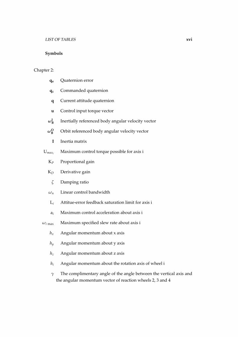
Symbols
Chapter 2:
qe Quaternion error
qc Commanded quaternion
q Current attitude quaternion
u Control input torque vector
ωIB Inertially referenced body angular velocity vector
ωOB Orbit referenced body angular velocity vector
I Inertia matrix
UmaxiMaximum control torque possible for axis i
KP Proportional gain
KD Derivative gain
ζ Damping ratio
ωn Linear control bandwidth
Li Attitue-error feedback saturation limit for axis i
ai Maximum control acceleration about axis i
ωi max Maximum specified slew rate about axis i
hx Angular momentum about x axis
hy Angular momentum about y axis
hz Angular momentum about z axis
hi Angular momentum about the rotation axis of wheel i
γ The complimentary angle of the angle between the vertical axis and
the angular momentum vector of reaction wheels 2, 3 and 4

LIST OF TABLES xvii
η A quater of the angle between the angular momentum vectors of re-
action wheels 2 and 3, 3 and 4 or 4 and 2 as seen from above
Chapter 3:
m Predicted mass of the satellite
R Predicted radius of the satellite
h Predicted height of the satellite
Ncommand Torque command sent to the BLDC controller
ωerr Angular velocity error
K1 Integrator gain 1 (equal to KP)
K2 Integrator gain 1 (equal to KPa)
a Position of the zero for wheel speed controller
B Magnetic field of the earth
H Reaction wheel angular momentum vector
M Torque vector exerted by magnetic torquers
k Magnetic controller gain
Chapter 4:
tPULSE BLDC controller Tacho output pulse width
RPUL Resistor value determining the Tacho output pulse width
CPUL Capacitor value determining the Tacho output pulse width
Rsense BLDC controller current sensing resistor
Ipeak Peak current delivered to the BLDC motor
PR Maximum power dissipated in the Rsense resistor
A Rate sensor (orthogonality) decoupling matrix
Ycr Average true roll angle of rotation (for four tests)
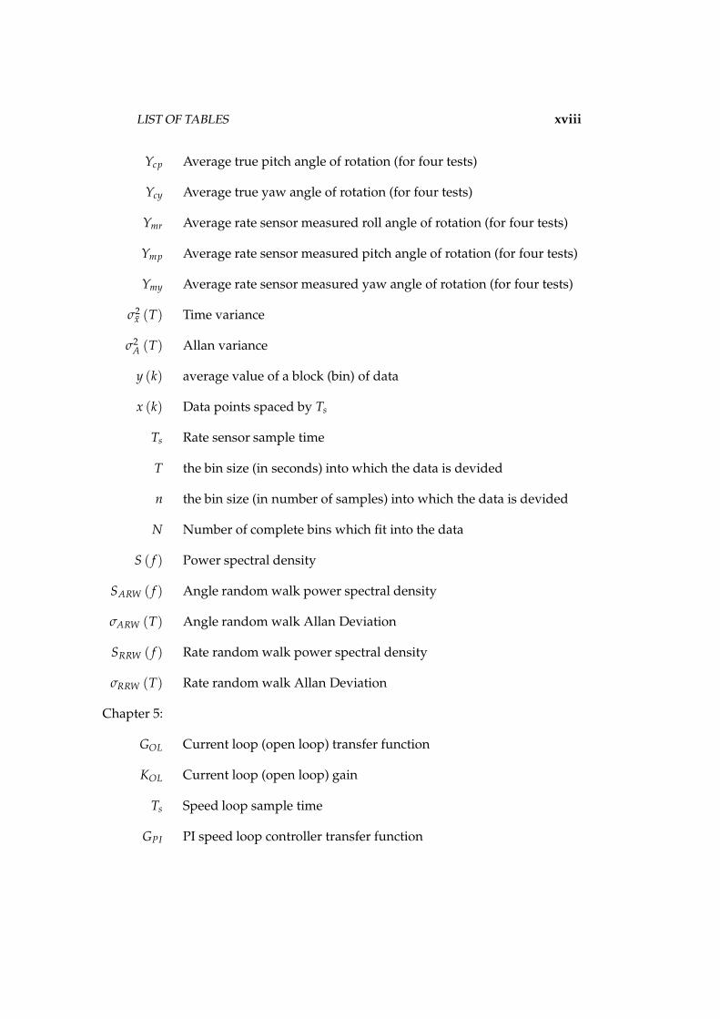
LIST OF TABLES xviii
Ycp Average true pitch angle of rotation (for four tests)
Ycy Average true yaw angle of rotation (for four tests)
Ymr Average rate sensor measured roll angle of rotation (for four tests)
Ymp Average rate sensor measured pitch angle of rotation (for four tests)
Ymy Average rate sensor measured yaw angle of rotation (for four tests)
σ2x (T) Time variance
σ2A (T) Allan variance
y (k) average value of a block (bin) of data
x (k) Data points spaced by Ts
Ts Rate sensor sample time
T the bin size (in seconds) into which the data is devided
n the bin size (in number of samples) into which the data is devided
N Number of complete bins which fit into the data
S ( f ) Power spectral density
SARW ( f ) Angle random walk power spectral density
σARW (T) Angle random walk Allan Deviation
SRRW ( f ) Rate random walk power spectral density
σRRW (T) Rate random walk Allan Deviation
Chapter 5:
GOL Current loop (open loop) transfer function
KOL Current loop (open loop) gain
Ts Speed loop sample time
GPI PI speed loop controller transfer function

LIST OF TABLES xix
Chapter 6:
Tg Gravity gradient disturbance torque
µ Gravity constant of the earth
R Orbit radius (from centre of earth)
θ Maximum deviation of the z-axis from the local vertical
y Rate sensor output
b Rate sensor bias from random walk process
ωb RRW component noise
Q RRW covariance matrix
v ARW component noise
R ARW covariance matrix
ω True angular rate
Chapter 7:
PO Solar cell array output power
Pintensity Power intensity of sunlight
Asolarpanel Solar panel area
Psa Power generated by solar array during sunlight
Pe Power requirement during eclipse
Pd Power requirement during sunlight
Te Eclipse time of orbit
Td Sunlit time of orbit
Xe Efficiency of solar panel supply path
Xd Efficiency of battery supply path

LIST OF TABLES xx
Appendix A:
Pmax Maximum power consumed by motor
Vamax Maximum armature voltage
Iamax Maximum armature current
INL No load current of motor
Nconst Torque constant of motor
Nmax Maximum torque requirement
VRamax Maximum voltage over armature resistance
Ωterminal Terminal resistance of motor
E0max Maximum back EMF
ωconst Speed constant of motor
ωmax Maximum rotational speed requirement

Chapter 1
Introduction
The attitude determination and control system (ADCS) is the subsystem of
a satellite which is responsible for stabilizing and orientating the satellite in
the desired direction. It takes external disturbance torques into account and
compensates accordingly which means that the satellite will be 3-axis stabi-
lized. This is done by using a set of different sensors to measure the attitude
of the satellite with respect to a fixed coordinate system. The orientation of
the satellite is then changed or maintained by using the actuators of the satel-
lite.
1.1 Aims and Objectives
The aim of this masters project is to design and test a subset of the full ADCS,
sensors and actuators, of a nanosatellite. The challenge in designing such a
subsystem for a nanosatellite is that all parts of the system must be as small,
light and power efficient as possible. The first aim of the project was to sim-
ulate the reaction wheel system along with the model of a nanosatellite. The
second aim was to design and build a tetrahedral reaction wheel system for
a nanosatellite which will enable 3-axis stabilization of the satellite. This in-
cluded designing the driving electronics for the four reaction wheels, the four
rotors and the mounting structure. The third aim of the project was to design
and build a rate sensor system for a nanosatellite. The final aim was to test
these subsystems on an air bearing in a hardware-in-the-loop (HIL) simula-
tion. This means that a part of the simulation (in this case the reaction wheel)
was replaced with the actual physical component to test the hardware as if
1

CHAPTER 1. INTRODUCTION 2
it was in the real system. A control system was also designed to prove that
the reaction wheel system can be used along with the rate sensor system, in
an air bearing setup, to control the attitude of the setup along one free axis of
rotation.
1.1.1 Mission Objectives
The nanosatellite to be designed will be launched together with a mother
satellite, which will most probably be an earth observation satellite. The
nanosatellite will have a CMOS camera sensor as main payload and will be
used to take images and video data of the mother satellite. These images will
be used to monitor the mother satellite and provide visual images for the
following possible processes or error scenarios of the mother satellite: The
deployment of solar panels or a boom with a tipmass, satellite detumbling or
external mechanical problems. This nanosatellite will also once more demon-
strate formation flying, 3-axis stabilized flight and orbit rendezvous of two
satellites with different drag characteristics. One of the main objectives of this
mission is also to educate masters students at the University of Stellenbosch
in the field of Space Engineering.
1.2 Background
In the past much research has been done on the subsystems of microsatel-
lites at the University of Stellenbosch. The Electrical and Electronical depart-
ment hosts the Electronic Systems Laboratory (ESL) where South Africa’s
first satellite, SUNSAT-1 (Stellenbosch University Satellite) was built from
1991 to 1999. Currently masters students at Stellenbosch University are do-
ing research on various subsystems of a nanosatellite. This project will also
contribute to the bigger aim of developing a nanosatellite at the University
of Stellenbosch.
The reason why the project of building a nanosatellite is done in an university
environment, is due to the fact that it can be done in a relatively short period
of time and the costs associated with developing and launching a nanosatel-
lite are relatively small. Builing a nanosatellite provides the extra challenge
of minimizing all the subsystems of a satellite while providing the same func-
tionality.
CHAPTER 1. INTRODUCTION 3
Previous reaction wheels were built at the ESL by Laurentius Joubert (for
Sunsat) and Xandri Farr. These reaction wheels are much too big and too
heavy for a nanosatellite, therefore a smaller reaction wheel system was needed
which will meet the torque, weight and size requirements of a nanosatellite.
Therefore this project focuses exclusively on the ADCS of a nanosatellite. A
tetrahedral reaction wheel system was therefore designed to make the total
system even more compact.
Redundancy is an important part of any space mission. In this project it is
therefore also necessary to make provision for the possibility of a reaction
wheel failure in space. An extra reaction wheel is therefore added to the
system to provide continual 3-axis controllability even when one of the four
reaction wheels fails. The tetrahedral form of the reaction wheel structure
was chosen, because in this configuration the nett angular momentum is zero
when all four wheels are rotating at the same angular velocity. This makes
the control of the system simpler due to the fact that the reaction wheels will
be used at a constant offset wheel speed.
1.3 Document Layout
In Chapter 2 the theory behind the design decisions will be explained. The
control algorithms which were tested in simulation will be explained. Chap-
ter 3 will discuss the simulation of the nanosatellite ADCS. First the reaction
wheel will be simulated together with the satellite dynamics and then the
implementation of momentum dumping will be discussed. The design de-
cisions made will be motivated in Chapter 4. Some of the detail design of
the reaction wheel system and the rate sensor system will be discussed in
this chapter. The simulation and practical results will be shown in Chapter
5. These results include the following topics: The HIL simulation, the ex-
perimental air bearing setup and the rate sensor system. Lastly in Chapter
6 the conclusions of this project will be presented and recommendations for
further studies will be given.
Chapter 2
Theory
Design decisions can only be made on the basis of the underlying theory.
This chapter describes the theory which was needed to complete this project.
2.1 Space Mission Geometry
When designing an ADCS for a nanosatellite it is important to know where
and how this satellite will be used. This includes the specific orbit the satellite
will be launched into, for example the inclination and altitude of the orbit.
The specifications set for the ADCS will be based on the background theory
of space mission geometry which will be explained in this section.
2.1.1 Coordinate Systems
The roll, pitch and yaw angles (Figure 2.1) can be used to define the transition
between the spacecraft-fixed coordinate system (Figure 2.2) and the orbit ref-
erence frame (Figure 2.3). The roll axis is the rotation around the spacecraft
direction of velocity. The pitch axis is the rotation around the negative orbit
normal direction. Lastly the yaw-axis is the rotation around the nadir direc-
tion.
The spacecraft-fixed coordinate system is used as the common reference frame
for all on-board sensors and actuators and it is fixed to the center of mass
(COM) of the satellite. Its axis will be chosen such that certain features of
the satellite are orientated along one axis of the spacecraft-fixed coordinate
system. Since the nanosatellite will have a camera as main payload, it would
4

CHAPTER 2. THEORY 5
Figure 2.1: Roll Pitch Yaw
be natural for one axis to be in the direction of the camera lens. Along with
the other two axes it should constitute a Cartesian coordinate system.
Figure 2.2: Spacecraft Fixed Coordinate System
The orbit reference frame defines the coordinate system for the spacecraft-
fixed reference frame using the orbital elements. It is a spacecraft centered
coordinate system and it is used to calculate the attitude of the satellite rela-
tive to the earth. The z-axis of the orbit reference frame is always in the nadir
direction. The x-axis points in the satellite velocity direction and the y-axis

CHAPTER 2. THEORY 6
points in the negative orbit normal direction, as seen in Figure 2.3.
Figure 2.3: Orbit Reference Frame
The earth centered earth fixed (ECEF) reference frame is a right orthogonal
coordinate system and as the name states, its origin is at the center of the
earth. The z-axis is in the direction of the north pole, the x-axis is in the direc-
tion of intersection between the equatorial plane (0 degrees latitude) and the
Greenwich meridian (0 degrees longitude) and the y-axis is the cross product
between the z- and x-axis.
Lastly the earth centered inertial (ECI) reference frame is used for orbit sim-
ulation purposes as it is also the basis for the physical laws which hold in
space. To be able to use Newton’s laws for modeling a spacecraft in space, an
inertial coordinate system is needed as reference. The coordinate system is
fixed with respect to the direction of the vernal equinox and its origin is also
at the center of the earth, as is the case with the ECEF reference frame.
2.1.2 Orbit parameters
The orbit of the nanosatellite will depend on the orbit of the mother satellite
with which it will be launched. Assuming that the mother satellite will be

CHAPTER 2. THEORY 7
Figure 2.4: ECEF Reference Frame
Figure 2.5: ECI Reference Frame

CHAPTER 2. THEORY 8
a low earth orbit (LEO) earth observation satellite, it will have a polar sun-
synchronous orbit. Sun-synchronous orbits have a retrograde precession of
360 degrees per year, which will ensure that the satellite will pass over the
equator at the same local time every orbit. Sun-synchronous orbits are pos-
sible for polar orbits with the correct inclination and altitude. For altitudes
between 400 and 900 km the inclination must be 98 ±1 for the orbit to be
sun-synchronous.
2.2 Control Algorithms
In this section the different aspects of the satellite attitude control algorithms
which were tested will be discussed. The inputs to the controller are the
quaternion error and the orbit referenced angular velocity of the satellite. The
output of the controller is the reference wheel torque. The controller output
will then be sent to the reaction wheel model.
2.2.1 Quaternion feedback
The Euler angle parametrization suffers singularities at ±90 degree pitch an-
gles when converting from the spacecraft coordinate system to the orbit ref-
erence frame. To avoid this problem, the quaternion approach is used, which
has a 4-element vector definition without any singularities.
The quaternion error is calculated by using the current and the reference
satellite attitude in quaternion representation as shown in equation (2.2.1).

CHAPTER 2. THEORY 9
qe =
q4c q3c −q2c q1c
−q3c q4c q1c −q2c
q2c −q1c q4c −q3c
q1c q2c q3c q4c
q (2.2.1)
Where,
q =[
q1 q2 q3 q4
]T
= Current quaternion (attitude)
qe =[
q1e q2e q3e q4e
]T
= Quaternion error
qc =[
q1c q2c q3c q4c
]T
= Reference (commanded) quaternion attitude
The quaternion feedback is a method which makes use of this quaternion
error to calculate the error between the reference attitude and the current at-
titude of the satellite. This quaternion error is an input to the controller along
with the orbit referenced satellite angular velocity to be able to calculate the
control torque vector as the output of the controller.
2.2.2 PD control
Euler’s rotational equations of motion of a rigid spacecraft, as discussed in
Wie [18], is repeated here (2.2.2) for the sake of completeness.
u = IωIB + ω
IB × Iω
IB (2.2.2)
Where,
u = control torque input vector
I = inertia matrix
ωIB = inertially referenced body angular velocity vector
A PD controller is used to control the reaction wheels of the satellite. The qua-
terion feedback controller for eigenaxis rotations, as discussed in Wie [18],
was used in this project. The controller proposed by Wie [18] counteracts the
gyroscopic term of Euler’s rotational equation. However for most practical

CHAPTER 2. THEORY 10
rotational maneuvers the gyroscopic term is small and can be neglected. The
control algorithm used in this project is shown in equation (2.2.3). The inputs
of the controller are the quaternion error vector and the orbit referenced body
angular velocity vector. The output of the controller is the control torque vec-
tor which is the input of the reaction wheel system. P and D are the controller
gain matrices to be properly determined.
u = satU max i
(
Pqe + DωOB
)
(2.2.3)
Where,
Umaxi= Maximum control torque possible for axis i
P = KPI
KP = 2ω2n (2.2.4)
= Proportional gain
I = Moment of inertia matrix
qe = Quaternion error
D = KDI
KD = 2ζωn (2.2.5)
= Derivative gain
ωOB = Orbit referenced body angular rate vector
ζ = damping ratio
ωn = linear control bandwidth
Variable limiter attitude error feedback
Wie [19] discusses an improvement on the control algorithm in equation
(2.2.3). A variable limiter attitute error feedback is included in the controller.
This improves the sluggish response (with increased transient overshoots)
while using the previous controller, when larger rapid maneuvers are done.
The slew rate limit needs to be adjusted for large commanded attitude an-
gles. The improved controller is shown in equation (2.2.6). The improvement
of the new controller is due to the fact that actuator saturation is prevented
by implementing the attitude error feedback saturation. Wie [19] claims that
the response using the improved controller is less sluggish and does not have
a transient overshoot. The gyroscopic term of the Euler rotational equations

CHAPTER 2. THEORY 11
of motion is also neglected in this controller assuming it to be small for all
practical rotational maneuvers.
u = satU max i
P satLi
(qe) + DωOB
(2.2.6)
Where,
Li =
(
KD
KP
)
min
[
√
4ai |qei| , |ωi|max
]
(2.2.7)
= Attitue-error feedback saturation limit for axis i
ai = U/Ii
= Maximum control acceleration about axis i
qei = Quaternion error for axis i
ωi max = Maximum specified slew rate about axis i
2.3 Tetrahedral Configuration
A tetrahedron is a triangular pyramid, which means that it is a polyhedron
composed of four triangular faces, three of which meet at each vertex, as can
be seen in Figure 2.6. A regular tetrahedron is one in which the four triangles
are equilateral. For the reaction wheel configuration designed the triangles
will all have side lengths of 60 mm. Using a tetrahedral shape mounting
structure means that four equal momentum vectors, perpendicular to each
side of the tetrahedron, amounts to a null momentum vector when they are
added together.
2.3.1 Conversion Matrix
A conversion matrix is needed to convert the momentum vectors of each
reaction wheel in the tetrahedral configuration to the satellite coordinate sys-
tem. This is needed because the momentum vectors of the wheels are not
perpendicular to each other, but rather perpendicular to the planes of the
tetrahedral shape on which they are mounted. The angular momentum and
torque vectors of the four reaction wheels are shown in the spacecraft coor-
dinate system in Figure 2.7.

CHAPTER 2. THEORY 12
Figure 2.6: The Tetrahedron
Figure 2.7: Tetrahedral Configuration

CHAPTER 2. THEORY 13
The conversion from the wheel angular momentum (or torque) vectors to the
Cartesian coordinate system is shown in equation (2.3.1).
hwx
hwy
hwz
=
0 cos γ − cos γ sin η − cos γ sin η
1 sin γ sin γ sin γ
0 0 cos γ cos η − cos γ sin η
h1
h2
h3
h4
(2.3.1)
The conversion from the angular momentum (or torque) vectors in Cartesian
coordinates to the wheel angular momentum and torque vectors is given in
equation (2.3.2).
h1
h2
h3
h4
=
0 cos γ − cos γ sin η − cos γ sin η
1 sin γ sin γ sin γ
0 0 cos γ cos η − cos γ cos η
−2 sin γ (1 + sin η) 2 sin η 1 1
−1
hwx
hwy
hwz
0
(2.3.2)

Chapter 3
Simulation
This chapter discusses the complete simulation process. It starts off with ex-
plaining the different models used in the simulation. The chapter goes on to
discuss the simulation of the reaction wheel system. Thereafter the imple-
mentation of the reaction wheel control algorithm is shown. An explanation
of how momentum dumping was simulated follows in the next section. The
last section in this chapter discusses the PD control block which acts as the
attitude controller for the satellite.
MATLAB Simulink is used as simulation environment throughout this project.
The basis of the simulations used in this project was provided by Steyn [17].
The simulations were however for a microsatellite application and had to be
changed to resemble a nanosatellite. The changes included:
• Modifying the reaction wheel model to simulate the tetrahedral reac-
tion wheel system used in this project
• The speed loop and current loop transfer functions of the actual reac-
tion wheels were determined and entered into the model
• The nanosatellite MOI was estimated and entered in the simulation
• Magnetic dumping was incorporated into the simulation
• The reaction wheel control was changed to control the smaller reaction
wheels
14

CHAPTER 3. SIMULATION 15
3.1 Simulation Models
The full simulation includes the reaction wheel system model, the reaction
wheel controller, the magnetic dumping controller, the satellite model and
the obit model. This simulation can be seen in Figure 3.1. The different mod-
els and controllers used in this simulation will be discussed in further detail
in the rest of this chapter. The simulation time has been chosen as 8000 sec-
onds, which amounts to roughly one and a third times the orbital period.
Figure 3.1: Simulink Simulation
The simulation requires a model of the orbit of the satellite. The orbit model
is implemented in a S-function block, as seen in Figure 3.1. Using the satel-
lite model, the attitude, orbit and inertially referenced angular velocity of
the satellite can be determined. The desired satellite reference attitude is the
input to the simulation. The error between the reference attitude and the
current attitude is sent into the reaction wheel controller. The output of the
controller is a torque command which is converted to an angular momen-
CHAPTER 3. SIMULATION 16
tum reference (through an integration process) for the model of the reaction
wheels. The torque and momentum vector of each wheel is determined, us-
ing their non-linear models, and sent back to the satellite model.
3.1.1 Satellite Model
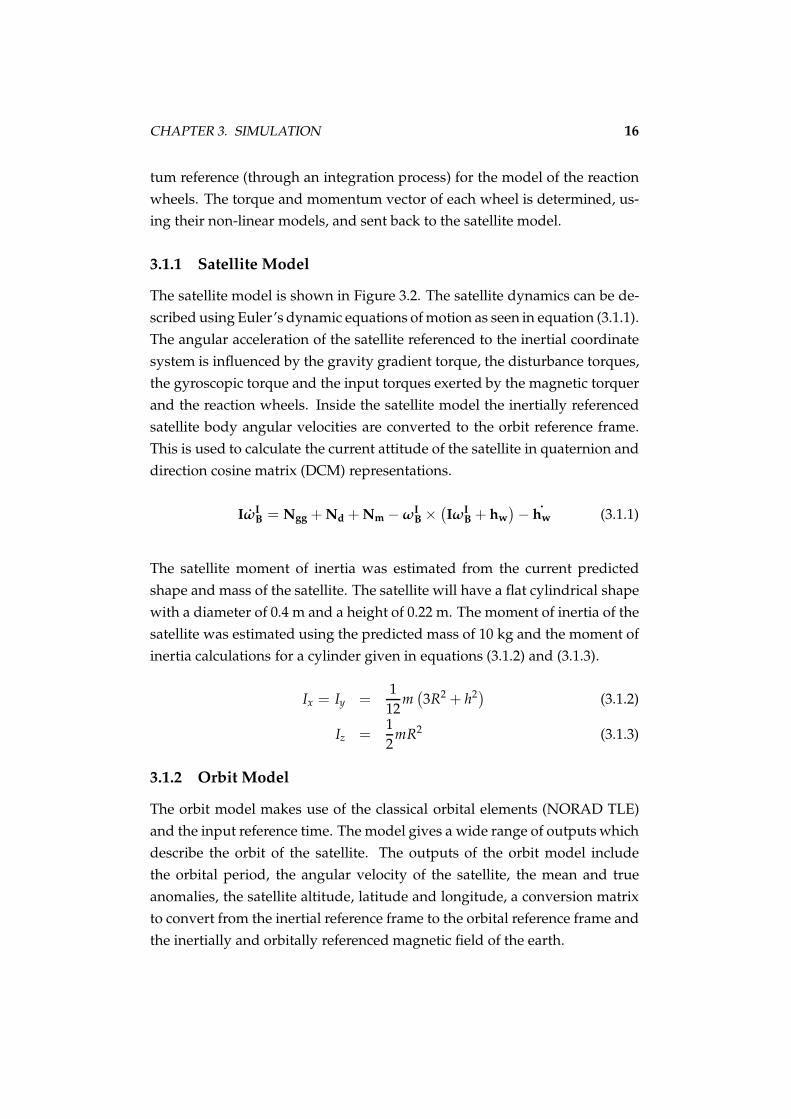
The satellite model is shown in Figure 3.2. The satellite dynamics can be de-
scribed using Euler’s dynamic equations of motion as seen in equation (3.1.1).
The angular acceleration of the satellite referenced to the inertial coordinate
system is influenced by the gravity gradient torque, the disturbance torques,
the gyroscopic torque and the input torques exerted by the magnetic torquer
and the reaction wheels. Inside the satellite model the inertially referenced
satellite body angular velocities are converted to the orbit reference frame.
This is used to calculate the current attitude of the satellite in quaternion and
direction cosine matrix (DCM) representations.
IωIB = Ngg + Nd + Nm − ω
IB ×
(
IωIB + hw
)
− hw (3.1.1)
The satellite moment of inertia was estimated from the current predicted
shape and mass of the satellite. The satellite will have a flat cylindrical shape
with a diameter of 0.4 m and a height of 0.22 m. The moment of inertia of the
satellite was estimated using the predicted mass of 10 kg and the moment of
inertia calculations for a cylinder given in equations (3.1.2) and (3.1.3).
Ix = Iy =1
12m
(
3R2 + h2)
(3.1.2)
Iz =1
2mR2 (3.1.3)
3.1.2 Orbit Model
The orbit model makes use of the classical orbital elements (NORAD TLE)
and the input reference time. The model gives a wide range of outputs which
describe the orbit of the satellite. The outputs of the orbit model include
the orbital period, the angular velocity of the satellite, the mean and true
anomalies, the satellite altitude, latitude and longitude, a conversion matrix
to convert from the inertial reference frame to the orbital reference frame and
the inertially and orbitally referenced magnetic field of the earth.

CHAPTER 3. SIMULATION 17
Figure 3.2: Satellite Model
3.1.3 Reaction Wheel System Model
A MATLAB Simulink simulation of the reaction wheel system of a microsatel-
lite (designed by Steyn [17]) was modified so that it could be used to simulate
the reaction wheel system of the nanosatellite designed for this project. The
reaction wheel system model includes 4 non-linear models of each reaction
wheel. One of the four identical non-linear models can be seen in Figure
3.3. The reaction wheel system model also includes the conversion matrix, as
seen in equation (2.3.1), which converts the four reaction wheel momentum
vectors to the satellite body coordinate system. In this model provision is
also made for the fact that the reaction wheels will be spinning at an offset
angular velocity of 1000 rpm. An offset wheel speed is used because an op-
tical encoder could not be used to determine the wheel speed and direction,
due to size constraints. As explained in more detail in section 4.4.1, the zero

CHAPTER 3. SIMULATION 18
wheel speed crossings therefore needed to be derived from the wheel speed
information. Using this particular offset wheel speed minimizes the zero an-
gular velocity crossings and therefore simplifies the wheel spinning direction
determination process.
Figure 3.3: Reaction Wheel Model
The non-linear model of each reaction wheel is made up of the following
components. At the centre of the non-linear model is the transfer function
model of the current loop which is closed inside the brushless DC motor con-
troller. The input to the current loop is the torque (which is related to the
current) reference supplied by the speed loop controller and the output is the
wheel angular momentum (which is related to the wheel speed). The current
loop is assumed to be much faster (more than 10 times) than the speed loop,
which is closed around the current loop. The transfer function of the current
loop is therefore simplified to a single integrator and an open loop gain. The
open loop gain is determined by plotting the wheel acceleration versus the
current command. This is done by conducting various tests where the wheel
acceleration is measured for different current commands. The wheel acceler-
ation divided by the current reference gives the constant open loop gain.
The second part of the non-linear reaction wheel model is the speed con-
troller which resides inside the 8051 microcontroller. It has a speed error in-
put and a torque command (in digital to analog units) to the BLDC controller

CHAPTER 3. SIMULATION 19
as an output. The transfer function of the discrete PI controller is shown in
equation (3.1.4). The calculation of the gains, Kp and Kpa, will be discussed
in section 5.2.
GPI(z) =KP(z − a)
z − 1(3.1.4)
The discrete control difference equation (3.1.5), which will later be used when
implementing the speed controller in the microcontroller, is derived from the
transfer function shown in equation (3.1.4).
u(k) = u(k − 1) + KPe(k) − KPae(k − 1) (3.1.5)
The non-linear reaction wheel model also includes the momentum and torque
saturation of each of the reaction wheels. The angular momentum buildup
on each reaction wheel is limited to 20 mNms (at 5000 rpm) and the torque
which can be exerted by each reaction wheel is limited to 5 mNm. The quan-
tization steps of the digital to analog converter is taken as 2.44 µNm (4096 bits
divided into a ±5 mNm range). Anti-integrator windup is also implemented
in this model to prevent the integrator from integrating the error when the
torque saturation limit has been reached.
3.1.4 Speed controller algorithm
The wheel speed controller is implemented in the microcontroller as shown
in equation (3.1.6). The design of this controller is discussed in section 5.2.
Speed reference commands can be given at 100 ms intervals, the speed con-
trol loop is executed inside the 8051 microcontroller at 10 times per second.
Therefore speed measurements are also done at these intervals. The previ-
ous torque command and the current and previous angular velocity errors
are used as inputs to the controller. The output of the controller is the torque
reference command which is converted to digital to analog units before it is
sent to the brushless DC controller. The integrator gains K1 and K2 are calcu-
lated (in section 5.2) according to the closed loop damping and settling time
specifications.
Ncommand(k + 1) = Ncommand(k) + ωerr(k + 1) ∗ K1 − ωerr(k) ∗ K2 (3.1.6)

CHAPTER 3. SIMULATION 20
3.2 Momentum dumping
Momentum dumping is the method of removing unwanted accumulated an-
gular momentum from the reaction wheels. This momentum buildup is due
to secular external disturbances on the satellite. Some of the secular dis-
turbance torques are caused by the earth’s magnetic field, gravitational and
aerodynamic influences on the satellite body. Momentum dumping is done
by using the magnetic torquers to create a torque in the opposite direction of
the angular momentum vector which needs to be dumped. This section will
discuss the algorithms which were used to implement momentum dumping
in the Simulink simulation.
The magnetic control block uses the B-field of the earth, as predicted by
the orbit propagation model, alongside with the reaction wheel angular mo-
mentum vectors in spacecraft body coordinates to calculate the torque which
needs to be exerted by the magnetic torquers. The algorithm used to calculate
this torque is shown below, in equation (3.2.1), where B is the earth’s mag-
netic field, H is the angular momentum of the reaction wheels in spacecraft
body coordinates, M is the torque exerted by the magnetic torquers and k is
the magnetic controller gain. The constant, k, must be negative, because the
torque generated by the magnetic torquers must be in such a direction so as
to decrease the momentum built up on the reaction wheels.
Equation 3.2.1 is obtained by assuming that the earth’s magnetic field, B,
is always perpendicular to the commanded magnetic dipole moment, M.
The components of the earth’s magnetic field (in the orbit reference frame)
are time-varying and depend on the orbit parameters (as discussed by Sidi
[13]). It is therefore not possible to make use of an analytic method to find
the correct value of the controller gain k (in equation (3.2.1)). The optimal
value which was found to be k = −1, was therefore determined using the
“cut-and-try” method. The estimated magnetic torquer saturation value was
taken into account when the controller gain was designed. For the designed k
value the commanded magnetic moment stays within the specified magnetic
torquer saturation value for the simulated disturbance torques.
M = kH × B
|B|2 (3.2.1)

CHAPTER 3. SIMULATION 21
The results of the implemented momentum dumping control algorithm can
be seen in section 6.1.3. Momentum dumping can however only by done
when the magnetic field (B-field) vector of the earth and the momentum vec-
tor to be dumped are not in the same direction. This can be seen from the
cross product in equation (3.2.1). The cross product implies that the mag-
netic torque applied depends on the angle between the angular momentum
vector and the B-field of the earth, the magnetic torque is a maximum when
the angle is 90 degrees and zero when the angle is 0 degrees. Momentum
dumping is thus constrained by the position of the satellite in its orbit.
3.3 PD controller block
In section 2.2.2 the theory behind the PD controller was discussed. The gains
KP and KD were chosen using equations (2.2.4) and (2.2.5) and the closed loop
specifications as shown in equation (3.3.1). Inside the PD control block the
closed loop specifications, ζ and ωn, were implemented as constants which
can therefore be changed easily (as seen in Figure 3.4). The torque saturation
of 5 mNm is also implemented in this block. The torque command is inte-
grated using a discrete integrator, with a sample time of 1 second, to calcu-
late the momentum reference which is sent to the reaction wheel model. This
satellite attitude controller is closed at 1 Hz, which is the reason for the inte-
grator sample time of 1 second. This sample time is therefore slow enough to
incorporate reaction wheel speed loop controller which is closed at 10 Hz.
ts 5% =3
ζωn(3.3.1)
= five percent settling time
3.3.1 Variable limiter attitude error feedback controller
The improved PD controller as discussed in section 2.2.2 is now implemented
in the simulation. The only difference between the previous (Figure 3.4) and
the improved PD controller is the fact that the quaternion error feedback is
limited. From Wie [19] it follows that, as the quaternion error increases, the
slew rate limit increases for rapid and large maneuvers. This means that the
overall response becomes sluggish and has an increased transient overshoot
because the actuator is saturated. To achieve improved settling times for

CHAPTER 3. SIMULATION 22
Figure 3.4: PD satellite attitude controller
large maneuvers the slew rate limit is adjusted as showed in equation (2.2.7).
The variable limiter insures that the actuator is not saturated and it improves
the transient response for large maneuvers. The results of this improved con-
troller will be discussed and compared to the PD controller without attitude
error saturation in section 6.1.1.

Chapter 4
Hardware Design
In this chapter the detail design of the different actuators and sensors covered
in this project will be discussed. To start with, the design requirements of the
ADCS system will be explained. This includes all the actuator and sensor
specifications relevant to this project. Thereafter the mission objectives will
be stated and discussed. This will be followed by a full explanation of all
the design steps followed to complete the reaction wheel system and the rate
sensor system.
4.1 Requirements
Previous research at the ESL has been done by Bootsma [4], Ntsimane [10],
Baker [1], Greyling [8] on the subsystems of microsatellites, on which the cur-
rent research on the subsystems of nanosatellites is based. Therefore the main
aim of the current subsystems developed is to compact the improved tech-
nology into smaller and lighter final units. The biggest requirement of this
project is therefore to make the final product as small and as light as possible,
due to the fact that it will eventually be flown on a nanosatellite. Another re-
quirement that goes with the size constraint is the power constraint. Smaller,
lighter batteries and solar panels must be used on nanosatellites and there-
fore the subsystems of nanosatellites must be as power efficient as possible.
4.1.1 Reaction Wheel Specifications
Firstly each reaction wheel must be able to deliver a torque of 5 mNm. The re-
action wheels must also be able to store an angular momentum of 20 mNms.
23

CHAPTER 4. HARDWARE DESIGN 24
This means that the maximum angular velocity of each reaction wheel must
be 5000 rpm, while each wheel has a moment of inertia around the spinning
axis of 38.2 ×10⁻⁶ kgm2. The minimum speed command which each reaction
wheel must be able to follow is 50 rpm.
4.1.2 Rate Sensor Specifications
The aim of building this sensor was to determine whether it is in fact a fea-
sible sensor to use on a nanosatellite. The power usage and sensor drift was
analyzed and compared to other off-the-shelf components. It was only re-
quired to determine most accurate angular velocity measurements which can
be obtained from the rate sensors, this implies that the sensor drift must be
as low as possible.
4.1.3 Mission
This nanosatellite will be used as an inspection satellite to observe another
satellite (a mother satellite) which will be in close proximity. This means that
the nanosatellite’s main payload will be a camera to image the mother satel-
lite. It also means that the nanosatellite will have to be 3-axis stabilized to be
able to take these images. This requires reaction wheels for accurate attitude
control. Magnetic torquers will also be needed to dump the momentum on
the reaction wheels, because of momentum buildup due to external distur-
bance torques on the satellite. To be able to inspect all the sides of the mother
satellite, the nanosatellite will have to be in such an orbit so that it will or-
bit around the mother satellite. The rotation of the nanosatellite to keep its
camera facing the mother satellite will be controlled by the onboard ADCS.
The nanosatellite will be launched together with the mother satellite, but will
inevitably have different drag characteristics. Therefore the nanosatellite will
need a propulsion system to enable it to rendezvous with the mother satellite
and to make minor orbit adjustments.
4.2 Reaction Wheel Design
In this section the detail design of the reaction wheel will be discussed. Firstly
the decisions made during the design of the mounting structure will be ex-
plained, the choice of motor will be defended and the rotor design will be

CHAPTER 4. HARDWARE DESIGN 25
discussed. Lastly the process of designing the motor controller and micro-
controller electronics will be presented.
4.2.1 Structure
The reaction wheel system must be redundant and support a zero momen-
tum bias with offset wheel speeds, so the design decision was made to mount
the four reaction wheels in a tetrahedral formation. As explained in section
2.3 equal angular momentums of the four reaction wheels amounts to a nett
zero momentum vector. This allows each reaction wheel to spin at an equal
offset angular velocity of 1000 rpm while the nett momentum stays zero. Due
to this fact and the fact that the tetrahedral configuration occupies a smaller
volume than the pyramid configuration, the tetrahedral configuration was
chosen. The positive directions of the angular momentum vectors can be
seen in Figure 2.7.
The structure was chosen to be as small as possible and as rigid as possi-
ble to minimize structure vibrations during launch. The structure fits into a
figurative cube with dimensions 100 mm by 100 mm by 100 mm. A Solid
Edge drawing of the tetrahedral structure alone can be seen in Figure 4.1.
The smallest possible tetrahedral shape structure was chosen so as to allow
for the rotors to each have a diameter of 50 mm (which will be on the outside
of the structure). The four brushless DC motors will be mounted in the cen-
ter of each of the four plates on the inside of the structure and their axes, on
which the rotors will be mounted, will be protruding from the structure as
can be seen in Figure 4.2.
The structure can be fully disassembled into 4 plates and 3 standoffs (see Ap-
pendix A.1), when assembled all junctions of neighbouring pieces are held
together by two 2.5 mm bolts. It is necessary to be able to disassemble the
structure fully, because the motors are in such close proximity of each other
on the inside of the structure, when assembled, that they have to be fixed to
the plates before connecting the plates to each other. The four plates which
constitute the tetrahedral structure are also identical, as are the three stand-
offs, which simplifies the production. The plates were manufactured using
laser cutting technology which ensures accuracy. A method called stitching
(small slits cut by the laser) was used along the folding lines to ensure that

CHAPTER 4. HARDWARE DESIGN 26
Figure 4.1: Tetrahedral Structure
the position of the folds were accurate.
The reflective optical sensors, used to measure the rotational speed of the
rotors, are also mounted in a corner of each of the four plates. The distance
from the sensor to the rotor was chosen to provide optimal reflective surfaces
for the sensor to discriminate between the polished and black surfaces of the
rotor. The standoffs are mounted on the mounting plate, which serves as a
baseplate for the structure and a means to mount the structure and the PCB
to the satellite.
Due to the triangular shapes which are connected to each other to make up
the tetrahedral structure it can withstand large vibrational forces. This is one
of the reasons why this shape was chosen. The shape of the tetrahedral struc-
ture was therefore assumed to be rigid enough so as to be able to use 1.6 mm
aluminium, but further vibration tests would be necessary to verify this as-
sumption. Possibly 1.2 mm aluminium (or maybe even 0.9 mm) could suffice,
depending on the vibration specifications of the specific launch vehicle used
to launch the nanosatellite.

CHAPTER 4. HARDWARE DESIGN 27
Figure 4.2: Tetrahedral Structure with Motors
4.2.2 Rotor
The material used for the rotor was chosen to have a high density, so as to de-
crease the volume of the rotor. The other criterion for the material was that it
should be easily obtainable and relatively inexpensive. Therefore brass was
chosen. The moment of inertia of each rotor around the spinning axis was cal-
culated as 38.2 ×10⁻⁶ kgm2 from the reaction wheel requirements. The rotor
diameter was designed to be 50 mm. The rotor has a cup like shape with 1
mm deep slits (1.2 mm wide) on its perimeter, which are used to determine
the rotational speed of the rotor, as seen in Figure 4.3. The only problem with
this material is the fact that it forms an oxidation layer in a short period of
time, which makes the surface dull. This reduces the reflectiveness of the
polished surface and the reflected signal coming from the diode is therefore
also weaker. This can lead to faulty speed readings and a sealant had to be
found to prevent this oxidation.
For the first design iteration it was chosen to machine 40 slits into the rotor.
This yielded a speed measurement resolution of 1.5 rpm at a 1 Hz sampling
frequency. Seeing that the satellite attitute control loop should ideally be
closed at 1 Hz, a faster sampling frequency for the speed measurement was

CHAPTER 4. HARDWARE DESIGN 28
Figure 4.3: The Brass Rotor
needed. A better resolution could only be obtained when more slits were
machined into the rotor. Therefore during the next design iteration it was
chosen to machine 72 slits on the side of each rotor, which would yield a
speed measurement resolution of 8.33 rpm at a faster sampling frequency of
10 Hz. This would allow the satellite attitude controller to run at 1 Hz. The
speed loop is therefore executed every 100 ms (as explained in section 3.1.4),
but the angular velocity is only displayed every second, thus with a resolu-
tion of 0.83 rpm. There was no speed measurement resolution requirement,
the resolution must only allow for the speed loop to be closed at 10 Hz. The
specific number of slits was chosen due to the fact that it was easier to ma-
chine slits into the rotor at integer angles (in this case 5 degrees). A better
resolution could be obtained by machining more slits on the perimeter of
each rotor, but the accuracy at which it could be machined would deteriorate
due to the machinery available. Therefore it was decided to keep to 72 slits
for this project until funding allowed a better machining process.
4.2.3 Motor
A brushless DC motor was chosen for this project, because the commutation
wear on a brushed DC motor is not desired for space applications. Three
small brushless DC motors were considered for this project, the 5.2 mNm
Faulhaber motor, the 13 W and the 6 W EC flat Maxon motor (see datasheets

CHAPTER 4. HARDWARE DESIGN 29
in Appendix B). The three key elements, on which the choice of motor was
made, were the size of the motor, its nominal operating voltage and the
power consumption of the motor. In the next 3 paragraphs these three crite-
ria will be discussed for each motor and the final decision will be motivated.
The maximum torque requirement for each motor is 5 mNm (according to
the specifications, see section 4.1.1). The power consumption, at an output
torque of 5 mNm and an angular velocity of 5000 rpm, of each motor was
therefore compared to each other. The power consumption under these op-
erating conditions of the Faulhaber motor is 5.65 W, the 6 W Maxon motor,
4.98 W, and the 15 W Maxon motor, 4.92 W (see Appendix B for calculations).
It can therefore be seen that the 15 W Maxon Motor has the smallest power
consumption by a small margin.
The size of the motor was to be as small as possible. This is why the EC-flat
series of Maxon motor was chosen above the Faulhaber motor. The brushless
DC motors in the EC flat series has an axial length of 28 mm in total, which is
a critical dimension in this compact design. The axial length of the Faulhaber
motor is 44 mm. Using this motor would enlarge the tetrahedral configura-
tion by a significant amount.
The nominal voltage also needed to be in the 12 V range, due to the smaller
power supply which will be used on the nanosatellite. Therefore the 6 W
Maxon motor with a nominal operating voltage of 9 V was chosen above the
15 W Maxon motor with a nominal operating voltage of 24 V.
It is therefore clear that, by taking all the above specifications in account,
the 6 W Maxon motor was the best choice of motor for this project.
4.2.4 Motor Drive Electronics
The motor drive electronics can be divided into 4 parts, the 8051 microcon-
troller and its components, the four brushless direct current (BLDC) con-
trollers and their peripheral components, the power distribution and com-
munications components. The schematics for these four parts of the motor
drive electronics can be seen in Appendix A.2.

CHAPTER 4. HARDWARE DESIGN 30
8051 microcontroller
The 8051 microcontroller has a 16 MHz crystal as clock source. This clock
source was chosen so that the CAN controller can operate at 1 Mhz, the UART
baud rate at 19200 baud and a timer can be set up to interrupt at 10 Hz for
the wheel speed control loop. External to the microcontroller a reset circuit is
set up to prevent small voltage drops in the power supply from resetting the
microcontroller. The serial peripheral interface (SPI) of the microcontroller
is used to communicate with an external digital to analog converter (DtoA)
which drives the references for the BLDC controllers. The inter-integrated
circuit (I2C) port of the microcontroller is used to interface with an external
analog to digital converter (AtoD), which converts the rate sensor outputs.
The Joint Test Action Group (JTAG) interface is used to program the micro-
controller. Four output pins on the microcontroller are used to drive the en-
able inputs of the BLDC controllers and another four output pins drive the
direction of rotation input pins on the BLDC controllers. Four input pins of
the microcontroller are configured as external timer inputs and act as coun-
ters to count the pulses from the optical reflective sensors, to determine the
rotational speed of the rotors.
BLDC controllers
The BLDC controller from ST Microelectronics (with component number L6235)
and its peripheral components have been chosen to fit the application. One of
the main requirements was that the controller should have an onchip three-
phase transistor bridge to drive the BLDC motors. This would minimize the
PCB space required for these components, as one controller would be needed
for each of the four BLDC motors. The other requirements for the controllers
are: It should be able to operate from a 12 V supply and it should be able
to deliver 0.7 A of current to the motor. The peripheral components for the
BLDC controllers include a charge pump, an external overcurrent and ther-
mal protection circuit, a current sense resistor, a PWM off time selection RC
circuit, a speed output pulse width selection RC circuit and bypass capacitors
and pull up resistors on the Hall sensor inputs.
The internal workings of the BLDC controller will now be discussed briefly
by taking a look at its block diagram as seen in Figure 4.4. The first is the

CHAPTER 4. HARDWARE DESIGN 31
constant off time PWM controller which makes use of an external RC circuit
to determine the off time. The external RC circuit has been chosen to give a
PWM switching frequency of between 8 kHz and 10 kHz (depending on the
on-time chosen by the controller). The optimal switching frequency would
be between 25 kHz and 40 kHz, but the choice was limited by the minimum
on time which is set by the controller.
Figure 4.4: BLDC controller Block Diagram
The second part of the BLDC controller consists of the three phase transistor
bridge which drives the BLDC motors. The current drawn by the BLDC mo-
tor is determined by measuring the voltage drop over a sense resistor which
is connected between the source of the three lower transistors in the bridge
and ground.
The tacho monostable uses the signal coming from the first Hall sensor to
output a pulse which length can be determined by an external RC circuit.
The BLDC motor uses an eight pole permanent magnet, which means that
four pulses per revolution can be measured and used to verify the speed out-
put coming from the reflective optical sensors. The pulse width is chosen to

CHAPTER 4. HARDWARE DESIGN 32
be short enough to accommodate the maximum rotational speed and long
enough to be registered on an input pin on the 8051 microcontroller. The
maximum rotational speed is 5000 rpm, resulting in the upper bound of the
pulse width of 3 ms and the lower bound set by the 8051 microcontroller
is 125 ns. A pulse width of 282 µs was therefore chosen and the resulting
resistor and capacitor values were calculated according to equation (4.2.1).
tPULSE = 0.6 × RPUL × CPUL (4.2.1)
The Hall-effect sensors decoding logic provides the appropriate driving of
the three-phase bridge outputs according to the signals coming from the
three Hall sensors. Lastly onboard the controller there are thermal protection
and overcurrent detection circuits to protect the controller against overheat-
ing and drawing too much current.
The sense resistor is chosen according to the peak current in the load and
there are two constraints to its resistance value. The first is that it dissipitates
energy due to the fact that all the current drawn by the BLDC motor flows
through this resistor and must therefore be kept as small as possible. The sec-
ond constraint is the fact that the voltage over the sense resistor is compared
to the reference voltage by the comparator; therefore the lower the sense re-
sistor value is, the higher the peak current error will be, due to noise on the
input reference voltage.
The recommended voltage drop over the sense resistor (according to the
datasheet) is 0.5 V when the peak current is flowing through it (see equation
(4.2.2)). The power rating of the sense resistor must also be taken into account
and can be calculated using equation (4.2.3). A resistance value of 0.733 Ω is
therefore chosen for the sense resistor, which is achieved by putting three 2.2
Ω resistors in parallel (the parallel combination insures that the power capa-
bility is adequate). The maximum torque required, of 5 mNm, results in the
maximum current of 0.7 A drawn by the BLDC motor. This was calculated
using the torque constant of the BLDC motor (according to its datasheet) and
determining the static and dynamic friction during operation. The required
power rating is therefore 0.36 W. Each of the 2.2 Ω resistors have a power rat-
ing of 200 mW resulting in a combined power rating of 600 mW which meats

CHAPTER 4. HARDWARE DESIGN 33
the requirement.
Rsense = 0.5/Ipeak (4.2.2)
PR = I2peak × Rsense (4.2.3)
Power Distribution
Three voltage levels are needed to supply the components on the Motor
Drive Electronics PCB. The BLDC controller needs a 12 V supply, the 8051
microcontroller needs a 3 V supply and the rest of the components need a 5
V supply. The 12 V supply which is connected to the PCB is regulated down
to 5 V using a switching regulator (with an efficiency between 86% and 95%
depending on the load and the input voltage). The 5 V supply is then regu-
lated to 3 V using a linear regulator.
Communications
The 8051 microcontroller communicates with the ground test computer us-
ing a serial UART connection. This communication is used to send the wheel
speed and rate sensor information to the ground test computer and to re-
ceive speed commands from the ground test computer, for demonstration
and ground testing purposes. The hardware for the CAN bus connection to
communicate with the on-board computer is also implemented. The SPI on
the 8051 microcontroller is used to communicate with the DtoA converter
which outputs an analog voltage to the voltage reference input on the BLDC
controller. The I2C connection on the 8051 microcontroller is used to commu-
nicate with the AtoD converter which converts the rate sensor data as stated
previously.
4.3 Rate Sensor Design
The design of the rate sensor system can be divided into 3 parts, the PCB
design, the mounting design and the calibration of the sensors. These three
design steps will be discussed briefly below. The rate sensors manufactured
by Analog Devices (with component number ADXRS401), which will be used
in this project, have a range of ±75 /s.

CHAPTER 4. HARDWARE DESIGN 34
Micro electromechnical (MEMS) gyros are usually designed as an electron-
ically driven resonator, often fabricated out of a single piece of quartz or
silicone, as described in Bijker [3]. The working of a MEMS gyro relies on
the Coriolis force that causes displacements of the resonator when an angu-
lar rate is applied to the sensor. These displacements can be detected by a
capacitive pickoff and demodulated to form the output of the sensor.
4.3.1 PCB design
The rate sensor system is divided into 4 parts, the three PCBs on which the
rate sensors are mounted, for the x, y and z-axis and the main gyro board,
which hosts the AtoD converter and the instrumentation amplifiers. The
schematics for these hardware designs are shown in Appendix A.3.1.
Three rate sensors are used per axis to be able to improve the estimation of
the true angular velocity. Thus on each of the three PCBs which are mounted
on the rate sensor mounting structure there are 3 rate sensors and their pe-
ripheral components, which includes a passive 20 Hz low pass filter. The
filter cut off frequency was chosen while considering the 100 Hz sampling
frequency. The design of this filter is discussed in Appendix A.4. The Nyquist
frequency (50 Hz) is therefore half of the sampling frequency and acts as the
upper bound for the low pass filter cut off frequency. This upper bound en-
sures that no aliasing occurs. The nominal output of the rate sensor is 2.5 V
and it deviates 15 mV per /s angular velocity. A full scale angular velocity
of ±15 /s is used for this satellite application. This means that the output of
the rate sensor will swing between 2.275 V and 2.725 V.
On the main sensor board instrumentation amplifiers are used to rescale the
rate sensor output signal to use a bigger range of the AtoD converter’s pos-
sible inputs. A 2 V reference is subtracted from the rate sensor output before
amplifying the signal by factor of 2. The minimum and maximum output of
the instrumentation amplifier will thus now be 0.55 V and 1.45 V respectively
for the full scale angular velocity outputs from the rate sensor. The AtoD con-
verter uses an internal reference of 2.048 V which means that the minimum
and maximum outputs of the AtoD converter will be 1100 and 2900 (DtoA
units) respectively. This means that a resolution of 16.67× 10⁻³ /s can be
obtained.

CHAPTER 4. HARDWARE DESIGN 35
4.3.2 Mounting structure
Firstly it is very important that the 3 surfaces on which the x, y and z rate
sensors will be mounted on must be orthogonal to each other. Care has thus
been taken in the manufacturing of the structure to respect this specification.
Secondly it was important that the structure should be as light as possible,
but materials which tend to outgas in space had to be avoided. Delrin was
thus chosen, because it is a strong material which is easy to machine and does
not outgas in space. A hollow cube was manufactured to save on weight,
leaving just enough of the frame of the cube to mount the three PCBs (see
Figure 4.5). The total weight of the structure is 9.4 g. Due to the fact that the
dimensions of the PCB to which the rate sensors are soldered are 22 mm by
32 mm, the Delrin cube has dimensions of 32 mm by 32 mm by 22 mm.
Figure 4.5: Rate Sensor mounting structure
4.3.3 Calibration
Before the rate sensors can be used they need to be calibrated. This proce-
dure includes calibration of the axis, the temperature output, the offset drift
due to temperature variation and determining the bias instability. Lastly the
initial conditions of the rate sensor output were recorded just after the power

CHAPTER 4. HARDWARE DESIGN 36
to the rate sensors were switched on. This will be used to calibrate the ini-
tial transients of the rate outputs due to the warming up of the rate sensors
internally. These procedures will be explained in the sections to follow.
Orthogonality
Two of the tree rate sensors were used per axis, which means that there are
effectively two sets of rate sensors which can be used to measure the angular
rates. These two sets will from here on be referred to as rate sensor set 1 and
2. The orthogonality calibration was done fixing the rate sensor system to
the inner gimbal of a turn table. Four tests per axis were performed, each
consisting of a 360 degree rotation around the particular axis. The angular
rate data was analysed by integrating the measured angular rates to obtain
an angular displacement measurement for both sets of rate sensors as seen in
Table 4.1 and 4.2. This measurement was then compared to the true rotation
angle of 360 degrees to calibrate the axis.
Table 4.1: Rate Sensor Calibration Measurements (set 1)
Experiment 1 Experiment 2 Experiment 3 Experiment 4
Roll Axis Test
Roll Axis 357.5396 361.6532 353.4244 361.3211Pitch Axis 0.0816 0.7392 0.9164 2.4368Yaw Axis 11.8473 12.1771 8.7964 14.7277
Pitch Axis TestRoll Axis 0.2990 2.1714 0.6660 2.7608Pitch Axis 363.9619 365.2805 362.9093 360.8096Yaw Axis 4.3880 1.5358 6.6809 1.5553
Yaw Axis TestRoll Axis 1.0037 2.9626 1.2215 2.3299Pitch Axis 0.8885 2.6775 2.4592 1.6639Yaw Axis 363.9620 364.9807 361.5431 359.3850
As can be seen from Tables 4.1 and 4.2 there is some cross coupling between
the roll, pitch and yaw axes. This cross coupling effect is due to the fact
that the sides of the mounting structure might not be perfectly orthogonal
to each other and the rate sensors might not have been soldered onto their

CHAPTER 4. HARDWARE DESIGN 37
Table 4.2: Rate Sensor Calibration Measurements (set 2)
Experiment 1 Experiment 2 Experiment 3 Experiment 4
Roll Axis Test
Roll Axis 347.8919 349.8659 339.7070 350.5748Pitch Axis 1.7944 0.5451 1.2360 1.3549Yaw Axis 14.2961 11.2277 8.2123 13.6768
Pitch Axis Test
Roll Axis 0.1142 1.6765 0.2184 0.7802Pitch Axis 346.8632 341.4480 348.7228 343.0313Yaw Axis 3.8859 2.7142 0.8585 1.1198
Yaw Axis Test
Roll Axis 5.9208 6.2102 10.3636 10.6652Pitch Axis 0.1456 1.2869 3.5055 0.7491Yaw Axis 364.5231 364.9161 359.3170 361.4272
respective PCBs very accurately. A decoupling matrix (A, as seen in equation
(4.3.1)) was calculated to correct these errors. The method of calculating this
decoupling matrix is shown in equation (4.3.2). This decoupling matrix is
then multiplied with the rate sensor measurements to obtain the true angular
velocities.
[
Ycr Ycp Ycy
]
= A ×[
Ymr Ymp Ymy
]
(4.3.1)
A =[
Ycr Ycp Ycy
]
× inv([
Ymr Ymp Ymy
])
(4.3.2)
Where,
Ycr = average true roll angle of rotation for the four experiments
Ycp = average true pitch angle of rotation for the four experiments
Ycy = average true yaw angle of rotation for the four experiments
Ymr = average rate sensor measured roll angle of rotation for the four experiments
Ymp = average rate sensor measured pitch angle of rotation for the four experiments
Ymy = average rate sensor measured yaw angle of rotation for the four experiments
A matrices (as seen in equation (4.3.2)) were calculated for both sets of rate
sensors. The results of these calculations can be seen in equations (4.3.3) for

CHAPTER 4. HARDWARE DESIGN 38
Table 4.3: Rate sensor biases for different temperatures
Temperature (C) 30 35 40 45 50
Rate sensor bias :(
10−3 × rad/s)
Roll 1 3.88 8.75 9.57 13.08 19.39Roll 2 -5.31 -11.35 -16.49 -21.94 -26.54Pitch 1 5.94 12.20 17.92 25.32 29.68Pitch 2 9.45 18.38 28.78 37.95 47.24Yaw 1 0.82 1.33 3.33 5.13 4.09Yaw 2 11.29 23.26 32.98 44.36 56.47
rate sensor set 1 and (4.3.4) for rate sensor set 2.
A1 =
1.0035 0.0006 0.0128
0.0025 0.9986 −0.0040
−0.0315 −0.0076 0.9940
(4.3.3)
A2 =
1.0389 −0.0042 0.0218
−0.0020 1.0446 0.0000
−0.0351 −0.0019 0.9956
(4.3.4)
Temperature
Firstly the temperature output of the rate sensor needed to be calibrated. This
is done by putting the rate sensors in a temperature controlled oven and cap-
turing the temperature output data at different known oven temperatures.
This data is then used to calibrate the temperature outputs of the rate sen-
sors. Then the angular rate output data of rate sensors during these tests is
used to calibrate the rate output bias offset due to temperature variation. Five
tests were completed at 30 C, 35 C, 40 C, 45 C and 50 C. The different
rate sensor biases for each test at a fixed temperature is given in Table 4.3.
Temperature calibration is essential for satellite applications due to the vary-
ing temperature in the space environment. The bias offset variation was
found to be in the order of 1.2×10⁻³ rad/s for a variation of 1 C as seen
in Table 4.4.

CHAPTER 4. HARDWARE DESIGN 39
Table 4.4: Rate sensor drift with temperature change
Rate sensor Roll 1 Roll 2 Pitch 1 Pitch 2 Yaw 1 Yaw2
Bias drift:(
10−3 × rad/s per C)
0.78 -1.06 1.19 1.89 0.16 2.26
Allan Variance
After performing the axis calibration tests, the bias drift of the Analog De-
vices rate sensor was found to be relatively large (in the order of 150 /h)
and therefore it needed verification that this bias drift was in fact due to the
bias instability of the rate sensor. This procedure will be explained in the next
paragraph.
Bias drift can be modeled as random walk, in other words the integration
of white noise. For a signal composed of a random walk process with addi-
tional white noise added (which is the case with the rate sensor signal), over a
short period of time the measured variance of the signal will be dependent on
the added white noise. However, over long periods of time, the random walk
process will begin to dominate. Allan Variance is a method of extracting the
variance of the white noise process driving the random walk, as well as the
variance of the added white noise. This is done be calculating the variance of
the sampled data as a function of averaging time. Time variance (TVAR) is a
form of Allan Variance (Cropp et al. [6]) and for discrete signals the TVAR is
the variance of the double difference of the mean of a block of data (as seen
in equation (4.3.5)).
σ2x =
1
6 (N − 2)
N−3
∑i=0
(
(
∆2 xi
)2)
(4.3.5)
Where,
∆2 xi = xi+2 − 2xi+1 + xi
The Allan Variance (as seen in equation (4.3.6)) technique as explained by
Bijker [3] was used in this project. It was used to determine the angle random

CHAPTER 4. HARDWARE DESIGN 40
walk and the rate random walk of each of the rate sensor outputs.
σ2A (T) =
1
2 (N − 1)
N−1
∑k=1
(y (k + 1) − y (k))2 (4.3.6)
Where,
y (k) =1
n
kn
∑i=(k−1)n+1
x (i)
x (k) = data points spaced by Ts
Ts = Sample time
T = nTs
= the bin size (in seconds) into which the data is divided
n = the number of data points over which
the average values were calculated
N = the number of complete bins which fit into the data
The relationship between the Allan variance and the power spectral density
of random processes (as seen in equation (4.3.7)) was used to determine the
power spectral density of the rate sensor signal from its Allan variance (Bijker
[3]).
σ2A (T) = 4
∫ ∞
0S ( f )
sin4 (π f T)
(π f T)2d f (4.3.7)
where S( f ) is the power spectral density (PSD) of a random process.
Rate sensor measurements were taken under certain fixed circumstances.
The rate sensor outputs must be stabilized (so as to eliminate the initial con-
ditions) and the rate sensor system must remain stationary. The Allan Vari-
ance technique was used to characterise the noise on the rate sensor output
signals. According to Bijker [3] the uncertainty in the sensor data can be as-
sumed to be generated by noise sources of specific character, as given below:

CHAPTER 4. HARDWARE DESIGN 41
1. Angle random walk
2. Rate random walk
3. Bias instability
4. Quantisation
5. Drift rate ramp
As stated in Bijker [3], the first two noise sources will dominate the noise on
MEMS devices. Therefore only these noise sources will be examined.
Angle random walk: The angle random walk is the measurement noise on
the rate sensor outputs which causes drift (random walk) on the integrated
rate sensor output signal. This noise can be approximated as white noise
with a angle random walk spectral density coefficient, Q, where the PSD is
given as:
SARW ( f ) = Q2 (4.3.8)
Substituting equation (4.3.8) into equation (4.3.7) (Bijker [3]):
σARW (T) =Q√
T(4.3.9)
Where the units of Q will be rad/s/√
Hz.
Rate random walk: The rate random walk drift on the rate sensor outputs
due to temperature differences and other external interferences. The PSD of
this noise is given in equation (4.3.10).
SRRW ( f ) =
(
K
2π f
)2
(4.3.10)
Substituting equation (4.3.10) into equation (4.3.7) (Bijker [3]):
σRRW (T) = K
√
T
3(4.3.11)
Where the units of K will be rad/s2/√
Hz.
Graphical representation: The calculated Allan deviation can be plotted
against averaging time on a log-log scale along with equations (4.3.9) and

CHAPTER 4. HARDWARE DESIGN 42
(4.3.11) which will appear as straight lines with inverse gradients. An exam-
ple of the Allan deviation vs averaging time plot for each of the rate sensor
outputs can be seen in Figure 4.6. The asymptote with the negative slope is
used to calculate the angle random walk value and the asymptote with the
positive slope, the rate random walk value. From this graph the values of
Q and K can be determined using equations (4.3.9) and (4.3.11). For short
window times, the angle random walk will be the most significant in the Al-
lan deviation value. These values will decrease for longer window times due
to the average being taken over more samples. At a certain point, the Allan
deviation will increase when the rate random walk is starting to dominate.
100
101
102
103
10−4
10−3
T[s]
Alla
n D
evia
tion
Allan Variance vs decimation ratio (Gyro Pitch 1)
100
101
102
103
10−4
100
101
102
10−4
10−3
T[s]
Alla
n D
evia
tion
Allan Variance vs decimation ratio (Gyro Roll 1)
T[s]
100
101
102
103
10−4
10−3
T[s]
Alla
n D
evia
tion
Allan Variance vs decimation ratio (Gyro Yaw 1)
100
101
102
10−4
10−3
T[s]
Alla
n D
evia
tion
Allan Variance vs decimation ratio (Gyro Yaw 2)
Allan Variance vs decimation ratio (Gyro Pitch 2)
Allan Variance vs decimation ratio (Gyro Roll 2)
Alla
n D
evia
tion
Alla
n D
evia
tion
100
101
102
10−4
10−3
T[s]
Figure 4.6: Allan Deviation vs averaging time
Initial conditions
The rate sensors used display an initial transient condition where, due to
the heating of the sensor internally, the biases of the output signals drift in a
certain direction. As previously stated the power resources on a nanosatellite

CHAPTER 4. HARDWARE DESIGN 43
are very limited. Therefore the rate sensors will only be switched on for very
short periods of time. The initial transients of each of the output signals was
thus recorded and will be used to calibrate the rate sensor outputs in the
initial state just after the power to these sensors has been switched on.
4.4 Integration
The integration of the reaction wheel system and the rate sensor system with
a hardware-in-the-loop (HIL) Simulink simulation will be discussed in this
section.
4.4.1 Reaction wheel system integration
The following parts of the reaction wheel system needed to be integrated
with each other: The structure, BLDC motors, the rotors, reflective optical
sensors and motor drive electronics and the 8051 microcontroller.
The reflective optical sensors were tested along with the 8051 microcontroller
to ensure that the correct angular velocity reading is calculated by the mi-
crocontroller. The direction of angular rotation must be derived from the
rotational speed readings using a predictive algorithm implemented on the
microcontroller. This algorithm uses the current and previous wheel speed
measurements to predict the wheel speed direction changes. This derivation
is needed, because the reflective optical sensor only has one output which is
high for a reflective surface and low for a non-reflective surface. No encoding
therefore exists to extract directional information.
When the rotors were integrated with the system and tested at a rotational
speed of more than 3000 rpm it was found that the vibrations due to un-
balanced rotors were significant and problematic for this application. Un-
der such circumstances the possibility exists of damaging the electronics and
sensitive sensors. It was therefore required to balance the brass rotors. It
was done using a simple technique of adding a small weight iteratively to
the rotor at different locations until the vibration was minimized. A hole of
the same mass as the balancing mass was then drilled on the opposite side of
the rotor. This process was repeated if the result was not satisfying until the
vibration was significantly damped at a rotational speed of 5000 rpm.
CHAPTER 4. HARDWARE DESIGN 44
The integration of the structure with the PCB hosting the motor drive elec-
tronics and the 8051 microcontroller, required a mounting plate, designed to
be as light as possible, but strong enough to withstand the vibrations during
launch. The mounting plate was machined from 1.6 mm aluminium, but fur-
ther research might show that a thinner aluminium plate may be sufficient.
4.4.2 Reaction wheel system and rate sensor system integration
The I2C communications interface of the 8051 microcontroller was required
to enable reception of the rate sensor data from the AtoD converter. A rate
sensor measurement update is sent to the microcontroller every 10 ms. This
data is then sent to the ground test computer via the UART interface. The raw
data is sent to the computer and it is therefore not calibrated in the 8051. The
main gyro board is supplied with 5 V and 3 V from the reaction wheel sys-
tem PCB. During this integration step it was also required to verify that the
8051 microcontroller is capable of executing all the software tasks timeously
(this includes I2C, SPI, UART communication and the rotor speed calcula-
tions). This was verified by using another timing device to determine the
time between wheel speed control intervals which was found to be 10 ms as
expected.

Chapter 5
Software Design
This chapter will discuss the software design for this project. At first a brief
overview of all the microcontroller software tasks will be given along with
a flow chart. Thereafter a detailed area of the software design will be dis-
cussed, namely the implementation of the wheel speed control algorithm.
5.1 Microcontroller code implementation
The main tasks of the 8051 microcontroller can be divided into 5 parts: The
rotational speed calculation and speed control of each of the 4 rotors, the I2C
communication with the AtoD (which converts the rate sensor data), the SPI
communication with the DtoA (which converts the reference voltage for the
BLDC controllers) and the UART communication with the ground test com-
puter (which is used to send speed reference commands and receive rotor
speed and rate sensor data). In this section brief commentary will be given
on the implementation of each of these tasks and which microcontroller re-
sources were used to fulfill these tasks.
5.1.1 Rotational speed calculation
To be able to determine the rotational speed of each of the rotors the pulses
from each of the reflective optical sensors need to be counted. A time refer-
ence is also needed to determine how many pulses are recorded in a certain
time. One of the 8051 timers are used for this purpose, it generates an inter-
rupt every 100 ms. Timers 2, 3, 4 and the programmable counter array (PCA)
timer are used as counters to count the pulses from the reflective optical sen-
45
CHAPTER 5. SOFTWARE DESIGN 46
sors. The values stored in the counters are used every 100 ms to determine
the rotational speeds of each of the rotors.
5.1.2 Speed control
The speed control implemented on the 8051 microcontroller is explained in
section 5.2. The speed loop is closed at 10 Hz. Additional checks are imple-
mented in the controller to ensure that variable overflows do not cause faulty
calculations. For this reason saturation checks of certain variables are imple-
mented. The maximum torque requirement and angular momentum which
is applicable for this project is also taken into account in the controller.
The wheel speed sign is determined by the controller onboard the 8051. The
previous speed reading is used together with the new reading to determine
whether the wheel speed is decreasing or increasing. When the wheel speed
is around zero this information is used together with the wheel speed ref-
erence to identify the changes in the wheel speed direction, seeing that the
reflective optical encoder only supplies magnitude readings and not direc-
tion.
When the wheel speed is below a certain threshold and the wheel speed refer-
ence is zero the current reference to the BLDC controller is zeroed. The static
friction is estimated using the minimum current reference which puts the
wheel into motion. The maximum torque command incorporates the motor
friction to ensure that the true maximum torque output of the BLDC motor
reaches the torque specification. The kinetic friction is assumed to be much
smaller than the static friction.
5.1.3 I2C communication
The I2C clock frequency is set at 220 kHz. This is done according to the mini-
mum low and high times for the I2C clock as specified by the AtoD converter.
There are twelve 12-bit values to be transmitted every 10 ms. This means that
24 data bytes (2 bytes per sampled channel) are needed to transmit the rate
sensor data and one additional byte is needed to transmit the slave address
of the AtoD converter. Between each transmitted byte there is an 18.2 µs
conversion period in which the AtoD converter converts the analog voltage.
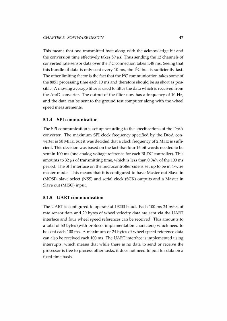
CHAPTER 5. SOFTWARE DESIGN 47
This means that one transmitted byte along with the acknowledge bit and
the conversion time effectively takes 59 µs. Thus sending the 12 channels of
converted rate sensor data over the I2C connection takes 1.48 ms. Seeing that
this bundle of data is only sent every 10 ms, the I2C bus is sufficiently fast.
The other limiting factor is the fact that the I2C communication takes some of
the 8051 processing time each 10 ms and therefore should be as short as pos-
sible. A moving average filter is used to filter the data which is received from
the AtoD converter. The output of the filter now has a frequency of 10 Hz,
and the data can be sent to the ground test computer along with the wheel
speed measurements.
5.1.4 SPI communication
The SPI communication is set up according to the specifications of the DtoA
converter. The maximum SPI clock frequency specified by the DtoA con-
verter is 50 MHz, but it was decided that a clock frequency of 2 MHz is suffi-
cient. This decision was based on the fact that four 16 bit words needed to be
sent in 100 ms (one analog voltage reference for each BLDC controller). This
amounts to 32 µs of transmitting time, which is less than 0.04% of the 100 ms
period. The SPI interface on the microcontroller side is set up to be in 4-wire
master mode. This means that it is configured to have Master out Slave in
(MOSI), slave select (NSS) and serial clock (SCK) outputs and a Master in
Slave out (MISO) input.
5.1.5 UART communication
The UART is configured to operate at 19200 baud. Each 100 ms 24 bytes of
rate sensor data and 20 bytes of wheel velocity data are sent via the UART
interface and four wheel speed references can be received. This amounts to
a total of 53 bytes (with protocol implementation characters) which need to
be sent each 100 ms. A maximum of 24 bytes of wheel speed reference data
can also be received each 100 ms. The UART interface is implemented using
interrupts, which means that while there is no data to send or receive the
processor is free to process other tasks, it does not need to poll for data on a
fixed time basis.

CHAPTER 5. SOFTWARE DESIGN 48
5.1.6 Flow chart overview
A flow chart depicting the sequence of tasks completed by the microcon-
troller is shown in Figure 5.1. It gives a brief overview of the sequence of
tasks which need to be executed by the 8051 microcontroller. The flow chart
shows the initialization stage and the main execution loop. The reaction
wheel speed control loop block will be discussed in more detail in section
5.2.
5.2 Implementation of wheel speed control algorithm
A proportional-integral (PI) controller is implemented on the 8051 microcon-
troller to control the wheel speeds of each of the four reaction wheels. The
form of the controller can be seen in equation (5.2.2). As stated previously,
the current loop is closed inside the BLDC controllers, it is assumed to be
much faster than the speed loop, which is closed at 10 Hz. Therefore the cur-
rent loop can be approximated using only an open loop gain (KOL) and an
integrator. This was confirmed to be a valid approximation through practical
measurements. Therefore only the open loop gain had to be determined to
complete the model of the current loop (see equation (5.2.1)).
GOL (s) =KOL
s
GOL (z) =KOLTs
z − 1(5.2.1)
GPI (z) =Kp (z − a)
z − 1(5.2.2)
This PI controller can now be written as a difference equation in the time
domain as in equation (5.2.3). This controller will then be implemented in
the microcontroller, with the controller gains K1 equal to Kp and K2 equal to
Kpa.
u (k) = u (k − 1) + Kpe (k) − Kpae (k − 1) (5.2.3)
The process of calculating the closed loop transfer function (of the speed
loop) can be seen in equation (5.2.4). The poles are placed according to the
design specifications, with a damping factor of 0.9 and a five percent settling
time of 0.53 s. This means that the poles of the second order system will
lie at −5.65 ± 2.74i in the s-plane. The controller gains, K1 and K2, can then

CHAPTER 5. SOFTWARE DESIGN 49
Figure 5.1: Flowchart of the tasks executed by the microcontroller

CHAPTER 5. SOFTWARE DESIGN 50
calculated as 11.12 and 8.31 respectively using equation (5.2.4) and the time
domain specifications.
GCL (z) =
Kp(z−a)z−1 × KOLTs
z−1
1 +Kp(z−a)
z−1 × KOLTsz−1
=KOLTsKp (z − a)
z2 −(
2 − KOLTsKp
)
z +(
1 − KOLTsKpa) (5.2.4)

Chapter 6
Results
In this chapter the outcomes which have been achieved will be discussed.
Explanations will also be given for the goals which could not be reached.
The first section in this chapter will give some simulation results which can
be compared to the real system at a later stage. Thereafter the reaction wheel
system in the simulation will be replaced with the real system and the results
of the hardware-in-the-loop tests will be shown. Lastly the results using the
experimental setup controller, designed to use the rate sensor feedback to
control the reaction wheel system, will be discussed.
6.1 Simulation Results
In this section the results from the simulation as discussed in Chapter 3 will
be given. Firstly it will be demonstrated that the PD controller implemented
performs as expected. Thereafter the inclusion of disturbance torques into
the simulation will be motivated and lastly the effectiveness of the momen-
tum dumping will be discussed.
6.1.1 PD controller
This section discusses the results of the PD satellite attitude controller as ex-
plained in section 3.3. The results which will be presented in this section
were obtained using the controller gains as stated in equation (6.1.1). The
algorithms for the controller gains in section 2.2.2 are repeated here to show
51

CHAPTER 6. RESULTS 52
how they were calculated.
ts 5% = 15s
ζ = 0.8
Therefore,
ωn = 0.25
KP = 2ω2n
= 0.125
KD = 2ζωn
= 0.4 (6.1.1)
Figure 6.1 shows that the reference attitude of the satellite is followed with
a 5% settling time of 13.85 s. In this example a reference roll angle of 30
degrees has been chosen. It can be seen that the actuators control the satellite
to follow this reference angle with little or no overshoot. The resulting five
percent settling time of 13.85 s is 1.15 s less than the specified settling time of
15 s. This is due to the fact that the three-axis quaternion feedback controller
is not linear. Similarly it can be shown that pitch and yaw reference angles
will be followed.
Variable limiter attitude error feedback results
The results for the improved PD controller (as discussed in section 3.3.1),
which implements a variable limiter for the attitude error feedback, will be
presented in this section. Figure 6.2 shows the different responses of the two
controllers. It shows that the controller which implements the limited atti-
tude error feedback has an improved transient response during large ma-
neuvers. For small angle maneuvers the two controllers, however, perform
similarly. It was therefore decided to use the simple PD controller (without
the attitude error limiter) in practise, because the responses of the two con-
trollers are equivalent for maneuvers up to 90 degrees. The added complexity
of the improved controller is also undesirable for this application.

CHAPTER 6. RESULTS 53
0 5 10 15 20 25 30−5
0
5
10
15
20
25
30
35
time [s]
Ang
le [d
eg]
Roll, Pitch and Yaw angles for a 30 degree Pitch rotation
rollpitchyaw
Figure 6.1: Simulation Result - reference attitude
0 20 40 60 80 100−40
−20
0
20
40
60
80
100
120
140
time [s]
Ang
le [d
eg]
Pitch angle for a 30 degree and 150 degree Pitch rotation
with variable limiterno error limitation
Figure 6.2: PD controllers with and without attitude error limitation compared
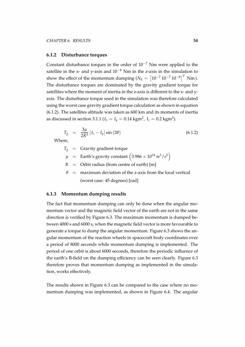
CHAPTER 6. RESULTS 54
6.1.2 Disturbance torques
Constant disturbance torques in the order of 10−7 Nm were applied to the
satellite in the x- and y-axis and 10−8 Nm in the z-axis in the simulation to
show the effect of the momentum dumping (Nd =[
10−7 10−7 10−8]T
Nm ).
The disturbance torques are dominated by the gravity gradient torque for
satellites where the moment of inertia in the z-axis is different to the x- and y-
axis. The disturbance torque used in the simulation was therefore calculated
using the worst case gravity gradient torque calculation as shown in equation
(6.1.2). The satellites altitude was taken as 600 km and its moments of inertia
as discussed in section 3.1.1 (Ix = Iy = 0.14 kgm2, Iz = 0.2 kgm2).
Tg =3µ
2R3
∣
∣Iz − Iy
∣
∣ sin (2θ) (6.1.2)
Where,
Tg = Gravity gradient torque
µ = Earth’s gravity constant(
3.986 × 10¹⁴ m3/s2)
R = Orbit radius (from centre of earth) [m]
θ = maximum deviation of the z-axis from the local vertical
(worst case: 45 degrees) [rad]
6.1.3 Momentum dumping results
The fact that momentum dumping can only be done when the angular mo-
mentum vector and the magnetic field vector of the earth are not in the same
direction is verified by Figure 6.3. The maximum momentum is dumped be-
tween 4000 s and 6000 s, when the magnetic field vector is more favourable to
generate a torque to dump the angular momentum. Figure 6.3 shows the an-
gular momentum of the reaction wheels in spacecraft body coordinates over
a period of 8000 seconds while momentum dumping is implemented. The
period of one orbit is about 6000 seconds, therefore the periodic influence of
the earth’s B-field on the dumping efficiency can be seen clearly. Figure 6.3
therefore proves that momentum dumping as implemented in the simula-
tion, works effectively.
The results shown in Figure 6.3 can be compared to the case where no mo-
mentum dumping was implemented, as shown in Figure 6.4. The angular
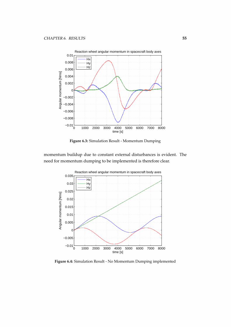
CHAPTER 6. RESULTS 55
0 1000 2000 3000 4000 5000 6000 7000 8000−0.01
−0.008
−0.006
−0.004
−0.002
0
0.002
0.004
0.006
0.008
0.01
time [s]
Ang
ular
mom
entu
m [N
ms]
Reaction wheel angular momentum in spacecraft body axes
HxHyHz
Figure 6.3: Simulation Result - Momentum Dumping
momentum buildup due to constant external disturbances is evident. The
need for momentum dumping to be implemented is therefore clear.
0 1000 2000 3000 4000 5000 6000 7000 8000−0.01
−0.005
0
0.005
0.01
0.015
0.02
0.025
0.03
0.035
time [s]
Ang
ular
mom
entu
m [N
ms]
Reaction wheel angular momentum in spacecraft body axes
HxHyHz
Figure 6.4: Simulation Result - No Momentum Dumping implemented

CHAPTER 6. RESULTS 56
6.2 Hardware-in-the-loop
The hardware-in-the-loop (HIL) simulation has one main objective, to prove
that the speed control loop implemented on the 8051 microcontroller behaves
as expected. This is done by comparing the angular velocity outputs of the
reaction wheels to the angular velocity outputs of the reaction wheel model,
while both the model and the real system are receiving the same inputs. This
will also serve as a method of verifying the accuracy of the reaction wheel
model.
In this chapter the changes made to the simulation as discussed in chapter
3 will be discussed. Then the interfacing between the Simulink simulation
and the 8051 microcontroller will be explained. Lastly this chapter will give
a summary of the results obtained from the hardware-in-the-loop tests.
6.2.1 HIL Simulation
Figure 6.5 presents the Simulink simulation model as used in Chapter 3. The
model has been changed to run the actual reaction wheel system in parallel
with its model to enable a comparison of their outputs and to verify the accu-
racy of the model. The HIL block is an S-function block which contains the C
code used to implement the communications protocol between the Simulink
simulation and the 8051 microcontroller. The inputs to the HIL block are the
wheel angular velocity references for each reaction wheel and the outputs are
the angular velocities measured from every reaction wheel.
Other than the added HIL block, convertion gains were required to convert
from the angular momentum reference output of the PD controller to the
wheel speed reference in rpm which is sent to the microcontroller. A con-
vertion method was also required for the wheel speed measurement, coming
from the microcontroller, to the wheel angular momentum and torque input
of the satellite model. The disturbance torques were removed from the simu-
lation along with the magnetic control implementing momentum dumping.
Seeing that the speed loop controller uses speed references in rpm units the
angular momentum reference values used in the simulation needed to be
converted to angular velocity values and scaled to the correct units. This was
done by firstly dividing the angular momentum values by the moment of in-

CHAPTER 6. RESULTS 57
ertia of the rotors and then converting them from rad/s units to rpm units.
Figure 6.5: Hardware-in-the-loop
The control of the actual reaction wheel system in this HIL simulation was
firstly done in an open loop fashion, using the reaction wheel system model
outputs as feedback to the satellite model. This was done to determine whether
the actual reaction wheel system was modelled accurately enough. The only
objective at this stage was therefore to compare the reaction wheel model and
the actual reaction wheel outputs.
6.2.2 Communications protocol
The protocol implemented to communicate between the ground test com-
puter and the 8051 microcontroller was designed to use ASCII characters to
represent the speed data, the direction of rotation and the reaction wheels
number. The contents of a single data packet is explained in Figure 6.6. This
was done in order to be able to interpret the ascii data without conversions
being necessary. Each wheel speed was also preceded by a unique character
to relate it to the specific wheel. The speed reference command sent to the
wheel microcontroller implements an absolute wheel speed command and a
CHAPTER 6. RESULTS 58
direction of rotation for each wheel. A current reference command was not
needed for this application and was therefore not implemented.
Figure 6.6: Communications protocol implementation
6.2.3 HIL results
Before the hardware-in-the-loop simulation could be implemented it was
necessary to prove that the reaction wheel model resembled the true reac-
tion wheel with small enough modelling errors to be able to insert the hard-
ware into the control loop. This was done by sending the same angular
velocity reference to both the reaction wheel model and the true reaction
wheel. The angular velocity, angular momentum and torque outputs of the
model and the true system were compared. The results, as seen in Figure
6.7, showed that the reaction wheel model was accurate enough to proceed
with the hardware-in-the-loop simulation. The small differences between
the model and the true reaction wheel outputs still eminent are due to the
fact that the effects of wheel friction (and air friction) are not included in the
model of the reaction wheel. That is why the model angular velocities dis-
play more overshoot at some stages during the simulation.
The reaction wheel model was then replaced by the actual reaction wheel in
the control loop. To compare the difference between the reaction wheel and
its model, a 30 degree pitch rotation was commanded using the actual reac-
tion wheel and the model in two separate simulations. The result is shown in
Figure 6.8. Figure 6.8 shows very small differences in the 30 degree reference
step response. These differences are due to small modelling errors (as ex-
plained above), seeing that identical satellite attitude controllers were used
in both simulations. The HIL simulation results showed a five percent set-
tling time of 13.6 s. The response when the model of the reaction wheel was
used for feedback showed a five percent settling time of 13.9 seconds. It can

CHAPTER 6. RESULTS 59
0 10 20 30 40
−500
0
500
1000
time [s]
Ang
ular
vel
ocity
[rpm
]
Wheel 1 ref, model and true angular velocity
referencemodeltrue
0 10 20 30 40
1000
1100
1200
1300
1400
1500
1600
time [s]
Ang
ular
vel
ocity
[rpm
]
Wheel 2 ref, model and true angular velocity
referencemodeltrue
0 10 20 30 40
1000
1100
1200
1300
1400
1500
1600
time [s]
Ang
ular
vel
ocity
[rpm
]
Wheel 3 ref, model and true angular velocity
referencemodeltrue
0 10 20 30 40
1000
1100
1200
1300
1400
1500
1600
time [s]
Ang
ular
vel
ocity
[rpm
]
Wheel 4 ref, model and true angular velocity
referencemodeltrue
Figure 6.7: Model and true RW system compared
therefore be seen that the results obtained from the two simulations (using
the model and the actual reaction wheel system for feedback) are very well
related. This also proves that the initial specification, requiring a 30 degree
rotation to be completed in less than 60 seconds, is satisfied in the simulation.
Figure 6.9 shows the angular velocity of the reaction wheel system compared
to its model in the simulation with a 30 degree pitch reference step, during a
hardware-in-the-loop simulation. The fact that Figure 6.9 and Figure 6.7 are
quite similar is also an indication that the model of the reaction wheel is quite
accurate. It is clear from Figure 6.10 that there are minor differences between
the damping coefficients of the actual reaction wheel system and the model
of the reaction wheel system. Smaller errors can be observed from the actual
reaction wheel response for bigger angular velocity steps. The reasons for
these differences will be discussed in section 6.4.1.
The angular momentum vector of wheel number one is aligned to the ver-
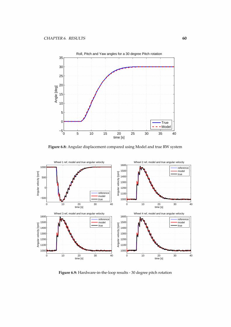
CHAPTER 6. RESULTS 60
0 5 10 15 20 25 30 35 40−5
0
5
10
15
20
25
30
35
time [s]
Ang
le [d
eg]
Roll, Pitch and Yaw angles for a 30 degree Pitch rotation
TrueModel
Figure 6.8: Angular displacement compared using Model and true RW system
0 10 20 30 40
−500
0
500
1000
time [s]
Ang
ular
vel
ocity
[rpm
]
Wheel 1 ref, model and true angular velocity
referencemodeltrue
0 10 20 30 40
1000
1100
1200
1300
1400
1500
1600
time [s]
Ang
ular
vel
ocity
[rpm
]
Wheel 2 ref, model and true angular velocity
referencemodeltrue
0 10 20 30 40
1000
1100
1200
1300
1400
1500
1600
time [s]
Ang
ular
vel
ocity
[rpm
]
Wheel 3 ref, model and true angular velocity
referencemodeltrue
0 10 20 30 40
1000
1100
1200
1300
1400
1500
1600
time [s]
Ang
ular
vel
ocity
[rpm
]
Wheel 4 ref, model and true angular velocity
referencemodeltrue
Figure 6.9: Hardware-in-the-loop results - 30 degree pitch rotation

CHAPTER 6. RESULTS 61
tical axis (pointing downward) which is the pitch axis of the actual reaction
wheel system. Wheels two, three and four are the wheels aligned at angles
of 70.53 degrees from the upward pointing vertical. From Figure 6.9 it can be
seen that the wheel one is accelerated in the opposite direction to wheels two
three and four to create the angular momentum in the pitch axis which will
turn the simulated satellite. The reaction wheel speeds converge back to 1000
rpm which means that the angular momentum exchange on the satellite will
be transferred back to the reaction wheels bringing the satellite to a standstill
at the end of the 30 degree pitch maneuver.
5 6 7 8 9 10
−500
0
500
1000
time [s]
Ang
ular
vel
ocity
[rpm
]
Wheel 1 ref, model and true angular velocity
referencemodeltrue
5 6 7 8 9 10
1000
1100
1200
1300
1400
1500
1600
time [s]
Ang
ular
vel
ocity
[rpm
]
Wheel 2 ref, model and true angular velocity
referencemodeltrue
5 6 7 8 9 10
1000
1100
1200
1300
1400
1500
1600
time [s]
Ang
ular
vel
ocity
[rpm
]
Wheel 3 ref, model and true angular velocity
referencemodeltrue
5 6 7 8 9 10
1000
1100
1200
1300
1400
1500
1600
time [s]
Ang
ular
vel
ocity
[rpm
]
Wheel 4 ref, model and true angular velocity
referencemodeltrue
Figure 6.10: Hardware-in-the-loop results - 30 degree pitch rotation (zoomed in)
Figure 6.11(a) shows the torque results in the x, y and z-axis for the hardware-
in-the-loop results. It is clear that the maximum torque of each of the four
wheels is combined to give a torque vector of around 10 mNm in the pitch
axis. Looking at the angular momentum in the x, y and z-axis in Figure
6.11(b) it can be seen that the pitch reference step causes the step in the angu-
CHAPTER 6. RESULTS 62
lar momentum of the reaction wheels in the y-axis and then the gradual re-
turn to a zero angular momentum to bring the simulated satellite to a stand-
still after the rotation.
6.3 Power, Mass and Size Budgets
Power
The specification was to minimize the power consumption of each of the
components used on the reaction wheel PCB as far as possible. Therefore
components with a low current usage were chosen. Some components can
also be switched off or switched to a low current state to save power. In
Table 6.1 the maximum current usage of each of the components is shown
according to the power supply voltage it uses. The table is divided into a sec-
tion where the datasheet current usage values are given and a section where
the measured values are shown. A total current usage for the total reaction
wheel system is also given for each power supply. Due to the fact that the 5
V regulator is powered from the 12 V supply the current drawn by the 5 V
regulator is included in the 12 V current usage. The same is true for the 5 V
supply and the 3 V regulator.
Examining Table 6.1 reveals that the total power consumption (1.77 W) of
the reaction wheel PCB is quite high for a nanosatellite application. The ini-
tial goal was for the power consumption to be less than 1 W in total. The
only solution to this problem would be to lower the power supply voltage.
Depending on the satellite bus voltage this would entail adding another volt-
age regulator which would add more power losses to the system. Tests were
done with lower supply voltages of 9 V and 8 V which lowers the power con-
sumption to 1.23 W and 1.09 W respectively.
Table 6.2 shows the total measured power consumption for the different op-
erating conditions stated. For each condition the calculated and measured
power consumption is given. The equation (B.0.1) used to calculate the power
consumption for the different operating conditions is discussed in Appendix
B. It can be seen that the calculated power consumption is lower than the
measured power consumption for each of the operating conditions. This is

CHAPTER 6. RESULTS 63
0 5 10 15 20 25 30 35 40−10
−8
−6
−4
−2
0
2
4
6
8x 10
−3
time [s]
Tor
que
[Nm
]
Reaction wheel torque for a 30 degree pitch rotation
NxNyNz
(a)
0 5 10 15 20 25 30 35 40−9
−8
−7
−6
−5
−4
−3
−2
−1
0
1x 10
−3
time [s]
Ang
ular
mom
entu
m [N
ms]
Reaction wheel angular momentum for a 30 degree pitch rotation
HxHyHz
(b)
Figure 6.11: (a) The reaction wheel torque and (b) angular momentum in the x, yand z-axis during a 30 degree pitch maneuver
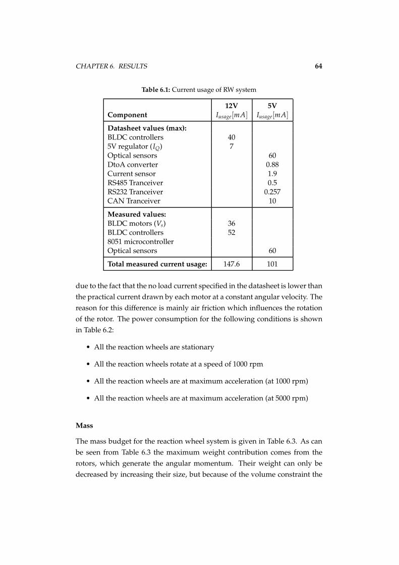
CHAPTER 6. RESULTS 64
Table 6.1: Current usage of RW system
12V 5V
Component Iusage[mA] Iusage[mA]
Datasheet values (max):
BLDC controllers 405V regulator (IQ) 7Optical sensors 60DtoA converter 0.88Current sensor 1.9RS485 Tranceiver 0.5RS232 Tranceiver 0.257CAN Tranceiver 10
Measured values:
BLDC motors (Vs) 36BLDC controllers 528051 microcontrollerOptical sensors 60
Total measured current usage: 147.6 101
due to the fact that the no load current specified in the datasheet is lower than
the practical current drawn by each motor at a constant angular velocity. The
reason for this difference is mainly air friction which influences the rotation
of the rotor. The power consumption for the following conditions is shown
in Table 6.2:
• All the reaction wheels are stationary
• All the reaction wheels rotate at a speed of 1000 rpm
• All the reaction wheels are at maximum acceleration (at 1000 rpm)
• All the reaction wheels are at maximum acceleration (at 5000 rpm)
Mass
The mass budget for the reaction wheel system is given in Table 6.3. As can
be seen from Table 6.3 the maximum weight contribution comes from the
rotors, which generate the angular momentum. Their weight can only be
decreased by increasing their size, but because of the volume constraint the

CHAPTER 6. RESULTS 65
Table 6.2: Measured power consumption of RW system
Condition Power usage [W] Power usage [W]
Measured Calculated
4 wheels stationary 1.774 wheels at 1000rpm 2.62 2.424 wheels (max accel, 1000 rpm) 11.77 10.54 wheels (max accel, 5000 rpm) 20.1 18.9
Table 6.3: Mass budget measured for RW system
Component Mass (g)
Structure 110.11Rotors 333.76BLDC Motors 128Optical sensors 4.6Mounting plate 51.22PCB 123.26
Total mass: 750.95
size of each of the reaction wheels is also limited. A compromise thus needed
to be found for the optimal size and weight of the reaction wheels. The other
significant contributions are made by the structure, the PCB and the BLDC
motors. Further improvements can be made using 1.2 mm (or maybe even 0.9
mm) aluminium to manufacture the structure after verifying that it is rigid
enough to withstand the vibration envorinment during launch.
Size
The size of the complete reaction wheel system is 110 mm by 110 mm by
130 mm high. The biggest contribution to the volume of the reaction wheel
system is the structure, which was designed to be as small as possible to
be able to house the BLDC motors on the inside. The depth and width of
the system was minimized to the size of the PCB, which itself was designed
to be as small as possible. The height of the system consists of the height
of the tetrahedral structure, the aluminium plate standoffs connecting the
structure to the base plate and the standoffs connecting the base plate to the
PCB. The height of the aluminium plate standoffs can be reduced by 1 cm
if they are redesigned to be the minimum height, which is the height of the

CHAPTER 6. RESULTS 66
rotor. Other than that the reaction wheel system was designed to occupy the
smallest possible volume.
6.4 Reaction wheel Measurements
This section will discuss some results regarding the reaction wheel system
as a whole and how effective it would be to use in a nanosatellite. The sec-
tion will also take the system requirements into account and discuss whether
they have been satisfied. The different subsystems of the reaction wheel sys-
tem will be discussed individually, and finally the system as a whole will be
evaluated.
6.4.1 Wheel speed control system
The reaction wheel controller was evaluated by comparing the results of the
reaction wheel model with that of the actual reaction wheel. The description
of the reaction wheel model was done in section 3.1.3. An angular velocity
reference step of 1000 rpm at 5 s and another 500 rpm at 10 s was given to
each reaction wheel of the true system, and their corresponding models. The
result is shown in Figure 6.12. It can be seen that the model and the true
reaction wheel follow the reference with five percent settling times of 1.24 s
and 1.15 s respectively. The other noticeable difference is the damping of the
true reaction wheel system which is much larger than that of the model. This
is due to the fact that the reaction wheel model does not incorporate wheel
friction and air friction. The dynamic friction of each the BLDC motors have
a damping effect on the step response. When the initial accelerations of the
reaction wheel model and the true system are compared, they are found to
be quite similar. These initial accelerations of the true reaction wheel and
the model can be calculated from Figure 6.12 as 128.68 and 134.17 rad/s2
respectively. This implies that the torque capability of each reaction wheel
modelled is accurate. The 0.1 s delay between the reference and the model
output is due to the fact that model output can only start changing after its
input, the reference wheel speed, has changed. The fact that the true wheel
speed is slightly smaller than the modelled wheel speed at any given time is
due to wheel and air friction as discussed above.

CHAPTER 6. RESULTS 67
0 5 10 15500
1000
1500
2000
2500
3000
time [s]
Ang
ular
vel
ocity
[rpm
]
Wheel 1 ref, model and true angular velocity
referencemodeltrue
0 5 10 15500
1000
1500
2000
2500
3000
time [s]
Ang
ular
vel
ocity
[rpm
]
Wheel 2 ref, model and true angular velocity
referencemodeltrue
0 5 10 15500
1000
1500
2000
2500
3000
time [s]
Ang
ular
vel
ocity
[rpm
]
Wheel 3 ref, model and true angular velocity
referencemodeltrue
0 5 10 15500
1000
1500
2000
2500
3000
time [s]
Ang
ular
vel
ocity
[rpm
]
Wheel 4 ref, model and true angular velocity
referencemodeltrue
Figure 6.12: Model and true system comparison: 1000 rpm speed reference step
6.4.2 Reflective optical sensors
The reflective optical sensors have been found to be adequate for the purpose
of wheel speed measurement. At the maximum wheel speed of 5000 rpm the
sensor is required to measure 6000 pulses per second and it does so effec-
tively. This means that the speed measurement resolution is 8.33 rpm when
measurements are taken every 100 ms (as discussed in section 4.2.2). The
only drawback of this sensor is its power consumption, it draws a minimum
of 10 mA of current from the 5 V supply. When the resistor which limits the
current to the infrared diode is increased the sensor fails to detect the slits in
the rotor. The power consumption for these four sensors therefore amounts
to 200 mW, which is problematic for a nanosatellite application due to the
limited power available.
6.4.3 Rotor
The rotors are unbalanced due to their manufacturing which is done locally
at a workshop at the university to save on manufacturing costs. The balanc-
ing of the rotors was also not done professionally, therefore small unbalances
could still remain. For the non-reflective surfaces to be detectable by the opti-

CHAPTER 6. RESULTS 68
cal reflective sensors a coating was required. This was done using an iodizing
process which leaves a black residue. This proved to be a sufficient method
in this application.
6.4.4 Microcontroller
The microcontroller needs to execute a few different tasks: Measuring and
controlling each of the four wheel angular velocities, UART, SPI and I2C
communication, as stated previously. It was proven practically that the 8051
microcontroller has sufficient processing power to execute all these tasks.
6.5 Rate sensor results
This section contains analysed test data which will be used to determine the
suitability of the Analog Devices rate sensors for space applications. Three
sets of data were used to verify the accuracy of the results. The results from
one set of data will be displayed in this section and the rest of the results
from the second and third sets of data can be seen in Appendix C. Figure 6.13
shows the recorded data from the six rate sensor outputs while the sensors
were at rest and kept at a fairly constant temperature.
The temperature influence will be discussed further in section 6.5.3. It is clear
that the measurement noise is quite significant, this shows in the covariance
results in section 6.5.4. The variance of the rate sensor outputs is in the order
of 4× 10⁻⁶ rad2/s2. The rate sensor outputs are firstly filtered using a passive
low pass filter with a cutoff frequency of 20 Hz. Thereafter the analog signal,
which is sampled every 10 ms, is converted to a digital signal using a 12 bit
analog to digital converter. The digital signal is then filtered using a moving
average filter, which means that the average of 10 samples is taken and the
filtered rate sensor data is sent to the ground test computer every 100 ms.
6.5.1 Allan Variance results
The first of the tests was to calculate the Allan Variance of each of the rate
sensor outputs. The seven hours of data as shown in Figure 6.13 was used for
this calculation. The Allan Variance technique, as explained in section 4.3.3,
was applied to retrieve the results as shown in Figure 6.14. The angle random

CHAPTER 6. RESULTS 69
Figure 6.13: Rate Sensor outputs over 7 hours
walk (ARW) and rate random walk values for each sensor as shown in Table
6.4 can be calculated from the graphs in Figure 6.14. This is done by using
equations (4.3.9) and (4.3.11) which represent the dotted lines on the left hand
side and right hand side, respectively, in Figure 6.14. The value of the angle
random walk can be obtained where the negative slope crosses T = 1 s and
the value of the rate random walk can be obtained where the positive slope
crosses T = 3 s. From Figure 6.13 it is clear that the measurement noise is
quite large (with variances in the order of 10−4 rad2/s2). The measurement
noise can be decreased using a higher order analog filter, in this application
only a passive first order analog filter was used.
6.5.2 Integrated rate sensor outputs
The rate sensor data was then integrated to give angular displacements. The
graph of angular displacements is shown in Figure 6.15 indicating maximum
angle random walk in the order of 30 radians over a 7 hour period. The
average drift was determined by calculating the drift over each 1 hour period

CHAPTER 6. RESULTS 70
Table 6.4: Angle Random Walk and Rate Random Walk values for the rate sensors
Rate Sensor ARW RRW(
1 × 10⁻⁴ rad/s/√
Hz) (
1 × 10⁻⁵ rad/s2/√
Hz)
Roll 1: 6.77 2Roll 2: 6.69 2.3
Pitch 1: 6.38 1.8Pitch 2: 7.46 1.2
Yaw 1: 6.26 0.95Yaw 2: 7.09 1.5
100
101
102
103
10−3.9
10−3.2
T[s]
Alla
n D
evia
tion
Allan Variance vs decimation ratio − Pitch 1
100
101
102
103
10−3.9
10−3.5
10−3.1
T[s]
Alla
n D
evia
tion
Allan Variance vs decimation ratio − Pitch 210
010
110
2
10−3.9
10−3.2
T[s]
Alla
n D
evia
tion
Allan Variance vs decimation ratio − Roll 1
100
101
102
10−3.9
10−3.2
T[s]
Alla
n D
evia
tion
Allan Variance vs decimation ratio − Roll 2
100
101
102
103
10−3.9
10−3.6
10−3.3
T[s]
Alla
n D
evia
tion
Allan Variance vs decimation ratio − Yaw 1
100
101
102
103
10−3.9
10−3.2
T[s]
Alla
n D
evia
tion
Allan Variance vs decimation ratio − Yaw 2
Figure 6.14: Allan Variance of the rate sensor outputs

CHAPTER 6. RESULTS 71
for every sensor and taking the average over all these periods. The result was
an average angular drift in the measured Euler angles of 203 degees per hour.
50 100 150 200 250 300 350 4000
10
20
30
time[min]
Pitc
h an
gle
[rad
]
Gyro Pitch output 1
50 100 150 200 250 300 350 400
−20
−15
−10
−5
0
time[min]
Pitc
h an
gle
[rad
]
Gyro Pitch output 2
50 100 150 200 250 300 350 400
−20
−15
−10
−5
0
time[min]
Rol
l ang
le [r
ad]
Gyro Roll output 1
50 100 150 200 250 300 350 400−10
0
10
20
time[min]
Rol
l ang
le [r
ad]
Gyro Roll output 2
50 100 150 200 250 300 350 400
−5
0
5
time[min]
Yaw
ang
le [r
ad]
Gyro Yaw output 1
50 100 150 200 250 300 350 400−30
−25
−20
−15
−10
−5
0
time[min]
Yaw
ang
le [r
ad]
Gyro Yaw output 2
Figure 6.15: Integrated rate sensor outputs
6.5.3 Filtered rate sensor outputs
The rate sensor outputs are filtered to retain the only the rate random walk
effect. The filter frequency is chosen from Figure 6.14, where the Allan devi-
ation value is at its smallest. This means that all the measurement noise will
be filtered out. The graph in Figure 6.14 reaches a minimum at an averaging
time of 500 s, which means that a filter frequency of 0.02 Hz must be used.
The filtered rate sensor output retaining only the rate random walk effect can
be seen in Figure 6.16.
The rate random walk is due to temperature changes and other effects in-
fluencing the rate sensor output bias. From Figure 6.17 it can be seen that

CHAPTER 6. RESULTS 72
50 100 150 200 250 300 350 400
−1
−0.5
0
0.5
1
x 10−3
time[min]
Pitc
h ra
te [r
ad/s
]
Gyro Pitch output 1
50 100 150 200 250 300 350 400
−5
0
5
x 10−4
time[min]
Pitc
h ra
te [r
ad/s
]
Gyro Pitch output 2
50 100 150 200 250 300 350 400
−5
0
5
x 10−4
time[min]
Rol
l rat
e [r
ad/s
]
Gyro Roll output 1
50 100 150 200 250 300 350 400−1
−0.5
0
0.5
1
x 10−3
time[min]R
oll r
ate
[rad
/s]
Gyro Roll output 2
50 100 150 200 250 300 350 400
−5
0
5
x 10−4
time[min]
Yaw
rat
e [r
ad/s
]
Gyro Yaw output 1
50 100 150 200 250 300 350 400
−1
−0.5
0
0.5
1x 10
−3
time[min]
Yaw
rat
e [r
ad/s
]Gyro Yaw output 2
Figure 6.16: Filtered rate sensor outputs - at cut off frequency of 0.02 Hz
the temperature variations during these tests were minimal, which means
that the rate random walk recorded was mostly due to the characteristics of
the sensor. The changes in the bias of the output of the rate sensors due to
temperature variation can be eliminated after calibration.
6.5.4 Rate sensor characterization
The rate sensor output can be modelled as the true angular rate added to
measurement noise (white noise) and a random walk process (integrated
white noise) as seen in equation (6.5.1). The measurement noise figure is
expressed in the covariance matrix of the rate sensor outputs and the ran-
dom walk process is described by the covariance matrix of the derivative of
the filtered rate sensor outputs. To identify the noise characteristics of this
sensor it is also required to be able to identify rate random walk and angle
random walk values for each of the sensors as seen in Table 6.4.

CHAPTER 6. RESULTS 73
Figure 6.17: Temperature outputs of rate sensors
y = ω + b + v (6.5.1)
Where,
y = rate sensor output
b = wb
b = rate sensor bias from random walk process
wb = RRW component noise
Q = Cov[wb]
= RRW covariance matrix
v = ARW component noise or measurement noise
R = Cov[v]
= ARW covariance matrix
ω = true angular rate

CHAPTER 6. RESULTS 74
The covariance matrix of the rate sensor outputs is shown in equation (6.5.2)
(with units of 1 × 10⁻⁵ rad2/s2).
R =
0.4113 −0.0038 −0.0030 0.0043 −0.0018 0.0018
−0.0038 0.3997 0.0082 −0.0017 −0.0013 0.0061
−0.0030 0.0082 0.3842 −0.0074 −0.0006 −0.0018
0.0043 −0.0017 −0.0074 0.5286 −0.0005 0.0049
−0.0018 −0.0013 −0.0006 −0.0005 0.3389 0.0005
0.0018 0.0061 −0.0018 0.0049 0.0005 0.4662
(6.5.2)
The covariance matrix of the derivative taken of the filtered rate sensor out-
puts (with units of 1 × 10⁻¹¹ rad2/s4) is shown in equation (6.5.3).
Q =
0.3139 −0.0323 0.0271 −0.0075 0.0015 0.0017
−0.0323 0.2821 0.0297 0.0086 0.0007 0.0260
0.0271 0.0297 0.4796 −0.0137 0.0151 0.0064
−0.0075 0.0086 −0.0137 0.2687 0.0074 −0.0041
0.0015 0.0007 0.0151 0.0074 0.2687 0.0154
0.0017 0.0260 0.0064 −0.0041 0.0154 0.3288
(6.5.3)
6.5.5 Rate sensor measurements improvement method
The rate sensors were the only feedback used during the experimental setup
(as seen in Figure 6.19) tests which were conducted. Due to the Euler an-
gle drifts on these sensors a possibility of improving the measurements us-
ing multiple sensors per axis was explored. An article by Bayard [2], which
implements a Kalman filter to combine the readings from each sensor, was
studied. It proved that a theoretical improvement of the angular rate mea-
surements was possible if the outputs of the sensors on each axis have a high
negative correlation factor. This proved not to be the case in practice, for
which reason this technique was not implemented.

CHAPTER 6. RESULTS 75
6.6 Control system - air bearing experimental setup
In this section the control system which is implemented as a Simulink simu-
lation (as seen in Figure 6.18), to control the attitude of the air bearing exper-
imental setup, will be discussed in detail along with its performance. At first
the air bearing experimental setup and the simulation will be explained and
thereafter the communications interface between the simulation and the reac-
tion wheel microcontroller. Then some results will be discussed, whereafter
the external disturbances will be taken into consideration.
Figure 6.18: HIL simulation - air bearing experimental setup
6.6.1 Air bearing experimental setup overview
The experimental setup as seen in Figure 6.19 is used to prove that the re-
action wheel system can be used, along with the rate sensors as feedback,
to control the attitude of the setup with one free axis of rotation at a time.
The experimental setup consists of 5 main parts. The level adjustable table is
used to ensure that the setup is level. The air bearings are used to create near
frictionless conditions for rotation in one axis. A metal bar placed on top of a
glass disk (which floats on top of the air bearings) is used to represent the mo-
ment of inertia of the nanosatellite. The reaction wheel system is also placed

CHAPTER 6. RESULTS 76
on top of the glass disk. To ensure that lateral disturbances do not push the
setup off the air bearings, a cable which is hung from the ceiling, is attached
to the reaction wheel system. The communications and power supply lines
also run along this cable. The cable only suspends some of the weight of the
reaction wheel system to ensure that minimum lateral movement and only
rotation takes place.
Figure 6.19: Experimental Setup
6.6.2 HIL simulation components
The hardware-in-the-loop simulation (as seen in Figure 6.18) can be divided
into four main parts. The first part is the hardware-in-the-loop block. It im-
plements the communication protocol which is used to communicate with
the 8051 microcontroller. The input to this block is the reference reaction
wheel speeds for each wheel and the output is the measured wheel speeds
and the rate sensor and temperature outputs. The second block is the rate
sensor calibration block. It implements the orthogonality, temperature and
initial conditions calibration of the rate sensor outputs. The third block is the
reaction wheel system block which is a model of the four reaction wheels.
CHAPTER 6. RESULTS 77
This block is used to compare the measured wheel angular velocities to the
predicted angular velocities in the reaction wheel model. The last of the four
main parts of the simulation is the PD controller. This implements the con-
troller which controls the attitude of the experimental setup in one axis at
a time. It makes use of a quaternion error input and the angular velocities
measured by the rate sensors. Its output is a reference angular momentum
for each of the four reaction wheels.
6.6.3 Moment of inertia
The moment of inertia of the air bearing experimental setup was determined
applying the law of conservation of momentum. The test was started while
all the reaction wheels and the experimental setup were stationary. The re-
action wheel in the vertical (pitch) axis is spun up to a fixed wheel speed.
Accoring to the law of conservation of momentum (equation (6.6.1)) the ex-
perimental setup will now have an equal opposite momentum. The rota-
tional speed of the setup is measured and used to calculate its moment of
inertia.
Irotor × ωrotor = Isetup × ωsetup (6.6.1)
The moment of inertia of the reaction wheel rotors therefore needed to be
determined accurately. This was done using a computer-aided design (CAD)
program and the string suspension method (as discussed in Appendix D)
to verify the accuracy of the result. The CAD analysis revealed a result of
36.8 ×10⁻⁶ kgm2 for the moment of inertia of the reaction wheel rotor. It
was found that there was a significant difference between the result using
the CAD program and the string method. It was decided that the CAD result
was more accurate (and reliable) and it was therefore used for further calcu-
lations.
A wheel speed of 3000 rpm (or 314.16 rad/s) was commanded for the reaction
wheel in the vertical (pitch) axis. This results in a wheel angular momentum
of 11.56 mNms. The experimental setup will therefore have an equal oppo-
site momentum, as discussed above. The angular velocity of the setup was
measured for 10 different tests and an average angular velocity of 2.459 rpm
(or 0.258 rad/s) was found. The moment of inertia of the air bearing experi-
mental setup was therefore determined as 44.9 ×10⁻³ kgm2.

CHAPTER 6. RESULTS 78
The moment of inertia used in the PD controller of the air bearing experi-
mental setup control system was therefore adjusted to the calculated value
for the setup.
6.6.4 Communications interface
Similar to the hardware-in-the-loop simulation a UART interface is used to
communicate with the 8051 microcontroller. A baud rate of 19200 bps is used
for this communication interface. The protocol is designed so that a speed
command can be sent every 100 ms to the 8051 microcontroller, while a mea-
sured wheel speed for each wheel along with the six rate sensor outputs and
the three temperature outputs is received from the 8051 microcontroller each
100 ms. The time of communication is however determined by the microcon-
troller so that the 100 ms interval between each data packet is accurate.
6.6.5 HIL control system results
Due to the HIL air bearing experimental setup the control system could only
be tested with one free axis of rotation. Some results will be given to prove
that the control system performed as expected in the particular axis of rota-
tion. Firstly the measured pitch Euler angle obtained by integrating the rate
sensor data can be seen in Figure 6.20(a). These measurements were taken
after giving a reference step pitch angle of 30 degrees at 25 s. The reference
angle step of 30 degrees is followed with a five percent settling time of 17
seconds. When compared to the specification of 30 degrees reference angle
step in less than 60 seconds it proves that the system satisfies its requirements
with quite a large margin.
When looking at the angular velocities of each of the four reaction wheels
(as seen in Figure 6.20(b)) it is clear that the maximum wheel speed of 5000
rpm is not exceeded. The build up (or loss) of angular momentum on each of
the wheels during standstill (between seconds 50 and 100) is due to external
disturbances mostly caused by the cable connected to the ceiling. This cable
ensures that the setup does not slide off the three air bearings.
The rate sensor angular and rate variations are now compared to the con-

CHAPTER 6. RESULTS 79
0 20 40 60 80 100−5
0
5
10
15
20
25
30
35
time [s]
pitc
h an
gle
[deg
rees
]30 degrees reference pitch angle step
(a)
0 50 100−1000
0
1000
2000
time [s]
whe
el s
peed
[rpm
]
wheel1 speed vs time
0 50 100500
1000
1500
2000
time [s]
whe
el s
peed
[rpm
]
wheel2 speed vs time
0 50 100500
1000
1500
2000
time [s]
whe
el s
peed
[rpm
]
wheel3 speed vs time
0 50 100500
1000
1500
2000
time [s]
whe
el s
peed
[rpm
]
wheel4 speed vs time
(b)
Figure 6.20: (a) 30 degree reference pitch angle step, (b) Reaction wheel angularvelocities during this maneuver

CHAPTER 6. RESULTS 80
trolled angular and rate variations (RMS), respectively, at a constant refer-
ence angle. This is done to determine the variation which is added by the
controller. This analysis gives another perspective on the efficiency of the
controller which is implemented.
Firstly the angular RMS values from the integrated rate sensor signal and
the controlled angle is measured. From Figure 6.20(a) a RMS angular vari-
ation, between seconds 50 and 100, of 0.352 degrees can be measured. The
measured RMS variation of the integrated rate sensor signal is 0.297 degrees.
From these values it can be seen that the controller adds a small amount of
RMS variation to the measured signal. The initial drift which can be seen in
Figure 6.21 is during the calibration time (during first 10 seconds). The offset
which is still emminent at 10 seconds in the simulation is therefore eliminated
after calibration and will not have an effect on the simulation.
0 20 40 60 80 100 1200
5
10
15
20
25
30
35
time [s]
Pitc
h an
gle
[deg
]
30 degree reference pitch angle step
Figure 6.21: Integrated rate sensor measurement of the 30 degree pitch maneuver
The rate variations are now calculated using the rate sensor signal and the
controlled rate. The satellite orbit referenced body angular rate is used to
find the controlled RMS rate variation. The controlled RMS rate variation
was calculated as 0.38 /s. The RMS variation of the rate sensor signal is

CHAPTER 6. RESULTS 81
measured as 0.47 /s. The reason why the RMS rate variation of the con-
trolled rate is smaller than that of the rate sensor signal is the fact that the
satellite attitude control loop is closed at 1 Hz and the rate sensor signal has
a frequency of 10 Hz. This means that the controller uses the average of 10
rate sensor measurements to control the attitude of the satellite. This brings
about the difference in rate RMS variation.
The last analysis looks at the RMS variation of the high pass filtered mea-
sured wheel speed signal. The highpass filtered wheel speed signals are
shown in Figure 6.22. The average RMS variation of the filtered wheel speed
signals is calculated as 62.99 rpm. This RMS variation shows that a large
amount of control input is used to keep the satellite stationary. A lower RMS
value would be preferable due to the smaller power consumption (at a con-
stant reference angle) it would have as a result. The variation in the wheel
speed can be decreased using either of the following two methods: The first
would be to use a rate sensor with less measurement noise and the other
method would be to design a controller with a lower bandwidth to be used
when no maneuvers are executed.
6.6.6 External disturbances
The external disturbances have unwanted effects on the experimental setup.
These disturbances are due to the cable suspended from the ceiling which
counters any lateral disturbances. The communication and power wires which
run along this cable also create disturbance torques. These disturbance torques
create a momentum buildup on the reaction wheels, which could cause the
momentum on the reaction wheels to saturate. The disturbances are however
small enough to be compensated for during a 100 second test period. It was
not possible to measure the magnitude of the disturbance torques due to the
fact that they vary depending on the angular position of the setup and the
position of the wires running along the cable. Air movement around the ex-
perimental setup could also cause disturbance torques, but they will be much
smaller than that of the disturbances caused by the cable and wires.

CHAPTER 6. RESULTS 82
60 80 100
−200
0
200
time [s]
whe
el s
peed
[rpm
]
wheel1 speed vs time
60 80 100
−100
0
100
time [s]
whe
el s
peed
[rpm
]
wheel2 speed vs time
60 80 100
−100
0
100
time [s]
whe
el s
peed
[rpm
]
wheel3 speed vs time
60 80 100
−100
0
100
time [s]
whe
el s
peed
[rpm
]
wheel4 speed vs time
Figure 6.22: High pass filtered wheel speed measurements of the 30 degree pitchmaneuver

Chapter 7
Conclusions and
Recommendations
This chapter will present some of the conclusions made after completing this
project. The conclusions will be divided into three sections. The first will dis-
cuss the effectiveness of the reaction wheel system to be used as actuator on a
nanosatellite. The second will entail the viability of the rate sensor for space
applications. The experimental setup will be evaluated critically discussing
the results obtained and how they can be improved. Lastly the outcomes will
be discussed in the light of the specifications given for each system evaluat-
ing their fulfillment of the goals set.
The recommendations part of this chapter will look at possible improvements
on each of the systems and subsystems designed. Recommendations will be
made for future work and classified in the order of importance.
7.1 Conclusions
7.1.1 Satellite simulation evaluation
The satellite model used in the simulation provides a platform on which the
reaction wheels could be tested as attitude actuators. Due to the fact that all
of the subsystems of the satellite are currently in the design phase, the actual
characteristics of the satellite, such as its size, weight and moment of inertia,
can only be estimated. The simulation can thus only be used to verify, using
the model of the reaction wheel and the estimated model of the satellite, that
83

CHAPTER 7. CONCLUSIONS AND RECOMMENDATIONS 84
the reaction wheel is an adequate actuator for the final satellite. The moment
of inertia values chosen for the nanosatellite model were estimated using a
flat cylindrical shape for the satellite, because it requires a small drag coeffi-
cient. This is why the moment of inertia in the vertical axis (z-axis) is larger
that in the lateral axes (x- and y-axis) as seen in equations (7.1.1), (7.1.2) and
(7.1.3). The estimated satellite dimensions are as follows: It has a height of
0.22 m and a diameter of 0.4 m, giving it a volume of 0.0276 m3.
Ix = 0.14 kgm2 (7.1.1)
Iy = 0.14 kgm2 (7.1.2)
Iz = 0.2 kgm2 (7.1.3)
It was therefore decided to use the real reaction wheel in the simulation by
conducting certain hardware-in-the-loop tests. These HIL simulations would
serve a double purpose, firstly it would eliminate the errors made by using
the model of the reaction wheel and secondly it could verify the reaction
wheel model.
Hardware-in-the-loop evaluation
During these simulations, as explained previously, the reaction wheel model
was replaced with the actual reaction wheel system. This served the purpose
of being able to design a controller to control the satellite attitude by using
the physical reaction wheel system. This simulation proved that the reaction
wheel performed as expected and the results showed that the torque and
momentum storage capability specifications were met. The closed loop spec-
ifications for the satellite attitude controller were also met using the actual
reaction wheel system as actuator.
7.1.2 Reaction wheel system evaluation
Torque and momentum storage capability
The specifications for each reaction wheel, of 5 mNm maximum torque and
20 mNms momentum storage capability, were met as stated above. This was
done using one of the smallest and most power efficient BLDC motors cur-
rently available on the market. Until more efficient products are available
the chosen motor suits this application best. These, above stated, specifica-

CHAPTER 7. CONCLUSIONS AND RECOMMENDATIONS 85
tions allow for a rotational maneuver of 30 degrees to be completed with a
five percent settling time of less than 20 seconds as shown in the HIL simu-
lation. The specification was therefore met, requiring a 30 degree maneuver
to be completed in at least 60 seconds. This is more than adequate for the
application as described in the mission objectives.
Size, mass and power usage
Seeing that the reaction wheel system was designed to be used on a nanosatel-
lite, some of the most important design specifications were its size, weight
and power usage. These specifications were however not fixed values, due
to the fact that the current technology available needed to be explored and
the smallest, lightest, most power efficient design was required. The results
of the system regarding these specifications were found to be quite viable for
its space application.
The total mass of 751 g is 7.5 percent of the maximum total satellite weight
of 10kg. This ratio is quite acceptable taking into account that the reaction
wheels contribute most of the weight of the ADCS and the proportional
weight of the ADCS of an average satellite is normally a tenth of the total
satellite mass. There is however still a margin for improvement in the weight
of the tetrahedral structure, due to the thickness of the aluminium used cur-
rently.
The size of 110 mm by 110 mm by 130 mm occupies about 6 percent of the
estimated total satellite volume of 0.027 m3. This ratio is adequate, especially
when taking into account that the on board electronics (such as the on board
computer) are becoming smaller with improved technology and will require
a smaller internal volume of the satellite.
A power analysis was done for the average consumption per orbit. It was
assumed that no maneuvers would be done in eclipse and two maneuvers
would be completed in the sunlit part of the orbit. These maneuvers would
entail a positive 30 degree off-nadir reference pitch angle step and a refer-
ence angle to return to the nadir position and another equivalent maneuver
in the negative 30 degree direction. Measurements were taken to determine
the average power consumption for a single 98.2 minute orbit expecting the

CHAPTER 7. CONCLUSIONS AND RECOMMENDATIONS 86
maneuvers, as explained above, to be executed. The estimated eclipse time
for the nanosatellite is 35 minutes and the period in the sunlit part of the or-
bit 63 minutes. The maneuvers are expected to last 17 seconds (see Figure
6.20(a) each. This means that for the rest of the orbit (97.1 minutes) the rotors
will be spinning at a constant speed of 1000 rpm. The power consumption
for the wheels to run at the nominal offset speed of 1000 rpm is 2.7 W (as seen
in Table 6.2). The average power consumption, over the 17 seconds it takes
to complete a 30 degree maneuver (in one direction), was measured as 6.36
W. This means that the average power consumption per orbit was estimated
to be 2.74 W.
A Lithium-Ion battery has a specific energy density of 70 - 110 Wh/kg, which
means that the storage capacity to support the nominal offset wheel speed of
1000 rpm should not be a problem (when a total battery mass of about 0.5 kg
is allowed).
The output power intensity of Silicon solar cells, at the beginning of their
lifetime, with the sun normal to the surface of the cells is 202 W/m2. The
cylindrical surface of the satellite (as discussed in section 7.1.1) facing the
sun will be 0.088 m2. Therefore the power generated by the solar cells (in the
sunlit part of the orbit) according to equation (7.1.4) is 17.8 W.
PO = Pintensity × Asolar panel (7.1.4)
The required power to be supplied by the solar cells, in the sunlit part of
the orbit, is determined using equation (7.1.5). The efficiencies of the voltage
supply paths from the solar cells (Xd) and the batteries (Xe) are estimated as
90% and 80% respectively. The time during eclipse (Te) and during the sunlit
part of the orbit (Td) are as discussed above. The power consumption during
daylight is estimated as 14 W and the consumption during eclipse, 10 W.
This estimation was done by assuming that the reaction wheel system power
consumption will be a fifth of the total power consumption during daylight
and that most of the other susbsystem will be switched to a lower power
mode during eclipse. According to equation (7.1.5) a solar array capable of

CHAPTER 7. CONCLUSIONS AND RECOMMENDATIONS 87
generating 22.5 W during the sunlit part of the orbit will be necessary.
Psa =
PeTeXe
+ PdTdXd
Td(7.1.5)
From the calculations, (7.1.4) and (7.1.5), it can be seen that the power re-
quired from the solar panels are higher than the power which can be gener-
ated by the Silicon solar cells. Solar cells with a higher efficiency (for example
Gallium Arsenide cells) will therefore be required for this nanosatellite. Im-
provement on the power consumption of the reaction wheel system might
also be necessary, which will decrease the average power usage per orbit.
Reaction wheel electronics
The BLDC controller (which has internal power MOSFET transistors) cho-
sen for this application was the most compact and power efficient controller
which could be found on the market. The maximum quiescent supply cur-
rent of 10 mA however makes a large contribution to the total power usage
(as seen in Table 6.1). It would be advisable to use a more power efficient
product when it becomes available.
The 8051 microcontroller on which the speed controller is implemented, proved
to have sufficient processing power for the tasks it is required to perform. Its
measured power usage of 90 mW is also a very small part of the total power
usage of the reaction wheel electronics (as seen in Table 6.1).
The voltage regulator used to convert the 12 V bus voltage to 5 V has a max-
imum efficiency of 95 percent at a load of 0.2 A. As shown by Table 6.1 the
regulator will however be used at a nominal load of 0.1 A, where the effi-
ciency will be 92 percent. The regulator used to convert from 5 V to 3 V was
however chosen to be a linear regulator (due to the fact that the output and
input voltage difference is small) and its efficiency will be lower.
7.1.3 Rate sensor system evaluation
The aim of testing the rate sensors was to determine whether they can be
used on a nanosatellite. It was found that the sensors have a bias stability of
203 degrees per hour or 3.4 degrees per minute. The sensors have an angular

CHAPTER 7. CONCLUSIONS AND RECOMMENDATIONS 88
random walk in the order of 7 ×10⁻⁴ rad/s/√
Hz. Comparing this to newer
rate sensors available on the market (for example the ADIS16250), the rate
sensors used in this project perform poorly. The ADIS16250, manufactured
by Analog Devices, has a bias stability of 57.6 degrees per hour or 0.96 de-
grees per minute. Its range of ±320 /s is four times larger than that of the
rate sensor used in this project. This means that the angular random walk
value as specified in the ADIS16250 datasheet, for the equivalent range of
the rate sensor used in this project, will be four times smaller. Its angular
random walk without digital filtering is therefore 2.5 ×10⁻⁴ rad/s/√
Hz for
a ±80 /s range. This means that after implementing the 10 Hz digital filter
as in the case of this project the ADIS16250 will perform much better than the
rate sensors used for this project.
When looking at the specification set for other space applications it is clear
that an angular random walk in the order of 5 ×10⁻⁵ rad/s/√
Hz and a bias
stability in the order of 100 degrees per hour is acceptable. In the 3-Axis mi-
cro gyroscope feasibility study done by Prezzavento [12] different rate sensor
application classes were compared, ranging from orbit control to failure de-
tection. The article determines the average required angular random walk
and bias stability for each of these classes. These specifications were used
to evaluate the characteristics of the rate sensors used in this project. These
values were also compared to the results from an article by Dussy [7].
It can therefore be concluded that the rate sensors used in this project are
not the best sensors currently available on the market and their performance
leaves a large margin for improvement. This sensor would not be adequate
for space applications and further research on other sensors, such as the
ADIS16250 would be necessary. The ADIS16250 was not available at the time
during the project when the rate sensors for this project was chosen.
7.1.4 Air bearing experimental setup evaluation
To evaluate the experimental setup it would be required to compare it to
the situation it simulates, when the satellite is in space. The fact that the
experimental setup only has one free axis of rotation limits the testing pos-
sibilities. The setup can however be tested in three orthogonal axes (during
three different tests by, changing the setup orientation) to prove that it would

CHAPTER 7. CONCLUSIONS AND RECOMMENDATIONS 89
perform as expected in a full three axis of rotation environment. The other
main drawback of the experimental setup is the disturbance torques exerted
by the stabilizing cable, communication and power wires connected to the
setup. The disturbances are different with each test, making it difficult to
analyse the true performance.
The experimental setup can thus be seen as a simulation of a satellite in space
with: One free axis of rotation at a time and large disturbance torques. If it
can be proven that the reaction wheel can be used successfully as actuator for
the experimental setup it will also perform well in space. The only difference
is that the maximum angular momentum will not be reached in such a short
time, due to smaller disturbance torques in space.
It was shown during the tests using the experimental setup that the reaction
wheel performed well, as the only actuator, over short periods of time. The
tests thus prove that the reaction wheel system will be adequate for space
applications on nanosatellites.
7.2 Recommendations
Regarding the reaction wheel system further improvements can be done in
the following areas:
• The size and weight of the structure can be improved
• The optical reflective sensors can be replaced with a more power effi-
cient sensor
• The number of slits on each rotor can be increased with a better ma-
chining process, to improve the speed measurement resolution
• The better machining process can be used for the manufacturing of the
rotors to eliminate unbalances or the wheels can be properly balanced
(static and dynamic)
Considering the rate sensor system the following improvements are recom-
mended:
• A more power efficient rate sensor with better bias stability and smaller
angle random walk characteristics must be found

CHAPTER 7. CONCLUSIONS AND RECOMMENDATIONS 90
• The analog filtering process must be done using an active filter, e.g., a
second order Butterworth filter
• A 16-bit in stead of a 12-bit analog to digital converter can be used
The improvements which can be made to the experimental setup to minimize
the external disturbances are as follows:
• The stabilizing cable can be replaced with a needle point rotational
setup
• The communication wires can be replaced with a wireless RS232 con-
nection
• Instead of the power cable Lithium Polymer (LiPo) battery cells can be
used as power source

Appendices
91

Appendix A
Hardware
A.1 Reaction wheel mounting structure assembly
The structure as shown in Figure 4.2 is assembled from six different parts.
Three baseplates as seen in Figure A.1(a) and three standoffs as seen in Figure
A.1(b). The different parts are connected to each other using 2.5 mm screws
and bolts. It was necessary to design the structure so that the BLDC motors
could be fixed to the baseplates before the structure is assembled, due to the
limited space inside the structure.
(a) (b)
Figure A.1: The reaction wheel structure (a) baseplate and (b) standoff
92
APPENDIX A. HARDWARE 93
A.2 Reaction wheel PCB schematics
In this section the PCB schematics will be given for the reaction wheel PCB.
The schematic for the BLDC drivers and peripherals includes the following
components:
• BLDC controllers and their peripheral components
• Connector for the optical encoders
• Connector for each BLDC motor
• Bypass capacitors for each voltage level
The schematic for the power distribution and communication includes the
following components:
• 5 V switching regulator
• 3 V linear regulator
• Power connector
• JTAG connector
• Current sense components for the 5 V power supply
• CAN controller with RS485 tranceiver
• RS232 tranceiver
The microcontroller schematic includes the following components:
• 8051 microcontroller
• Digital to analog converter and its reference voltage supply component
• Bypass capacitors for each of the voltage supplies
• LEDs to indicate that the voltage supplies are active
• 16 MHz crystal as external clock source for the 8051 microcontroller
• Reset circuitry

AP
PE
ND
IXA
.H
AR
DW
AR
E94
A.2
.1B
LD
Cd
rive
rs
1
1
2
2
3
3
4
4
5
5
6
6
D D
C C
B B
A A
Title
Number RevisionSize
B
Date: 2007/09/20 Sheet of
File: C:\Documents and Settings\..\BLDCdrivers.SchDocDrawn By:
A1
K2
D1
1N4148
R42.2
R1
100K
R32.2
C15.6nF
R9100K
Out1_1
Out1_1
Out2_1
Out2_1
Out3_1Out3_1
Hall1_1
Hall1_1
Hall2_1
Hall2_1
Hall3_1
Hall3_1
RCOFF_1
C61nF
R13150K
RCOFF_1
R11100
C410nF
D21N4148
VBOOT_1
VBOOT_1
C5220nF
En_1
Iref_1
FW_REV_1
DGNDDGND
DGNDDGNDTacho1RCPULSE_1
R8
10K
Tacho1
C710nF
R1447K
RCPULSE_1
C30.1uF
12V12V
DGNDDGND
SPD1
R22.2
R510K
R1010K
R1210K
R7
13K
R6
16K
Tacho_1
R165K6
R17
15K
5V5V
C29
10uF
C2100uF
C30
1uF
C31
0.1uF
D3
1N4148
R212.2
R18
100K
R202.2
C85.6nF
R26100K
Out1_2
Out2_2
Out3_2
Hall1_2Hall2_2Hall3_2
RCOFF_2
C131nF
R30150K
RCOFF_2
R28100
C1110nF
D41N4148
VBOOT_2
VBOOT_2
C12220nF
En_2
Iref_2
FW_REV_2
DGNDDGND
DGNDDGNDTacho2RCPULSE_2
R25
10K
Tacho2
C1410nF
R3147K
RCPULSE_2
C100.1uF
SPD2
R192.2
R2210K
R2710K
R2910K
R24
13K
R23
16K
Tacho_2
R335K6
R3415K
C9100uF
D5
1N4148
R382.2
R35100K
R372.2
C155.6nF
R43100K
Out1_3Out2_3
Out3_3
Hall1_3
Hall2_3
Hall3_3
RCOFF_3
C201nF
R47150K
RCOFF_3
R45100
C1810nF
D61N4148
VBOOT_3
VBOOT_3
C19220nF
En_3
Iref_3
FW_REV_3
DGNDDGND
DGNDDGND
Tacho3RCPULSE_3
R42
10K
Tacho3
C2110nF
R4847K
RCPULSE_3
C170.1uF
SPD3
R362.2
R3910K
R4410K
R4610K
R41
13K
R40
16K
Tacho_3
R505K6
R5115K
C16100uF
D7
1N4148
R552.2
R52100K
R542.2
C225.6nF
R60
100K
Out1_4Out2_4
Out3_4
Hall1_4Hall2_4Hall3_4
RCOFF_4
C271nF
R64150K
RCOFF_4
R62100
C25
10nF
D81N4148
VBOOT_4
VBOOT_4
C26220nF
En_4
Iref_4
FW_REV_4
DGNDDGND
DGNDDGNDTacho4RCPULSE_4
R59
10K
Tacho4
C2810nF
R6547K
RCPULSE_4
C240.1uF
SPD4
R532.2
R5610K
R6110K
R6310K
R58
13K
R57
16K
Tacho_4
R675K6
R6815K
C23100uF
DGND
Out1_2
Out2_2
Out3_2
Hall1_2
Hall2_2
Hall3_2
DGND
Out1_4
Out2_4
Out3_4
Hall1_4
Hall2_4
Hall3_4
DGND
Out1_3
Out2_3
Out3_3
Hall1_3
Hall2_3
Hall3_3
DGND
5V 5V
12V
5V 5V
5V 5V
12V
5V 5V
5V
12V
12V
5V 5V
5V
12V
12V
12V
12V
12V
12V
12V
12V
12V
12V
12V
12V
12V
12V
12V
12V
DGND
DGND
DGND
DGND
DGND
DGND
DGND
DGND
DGND
DGND
DGND
DGND
DGND
DGNDDGND
DGND
DGND
DGND
DGND
DGND
DGND
DGND
DGND
DGND
DGND
DGND
DGND
DGND
C72
1nF
C73
1nF
C71
1nF
DGND DGND
C70
1nF
DGNDC76
1nF
DGND
C79
1nF
DGND
C69
1nF
DGND
C78
1nF
DGND
C75
1nF
DGND
DGND
C68
1nF
DGNDC74
1nF
DGND
C77
1nF
DGND
Vdd11
SPD13
SPD412
Vdd410
GND411
GND12
Vdd24
GND25
SPD26
SPD39
GND38
Vdd37
opt1to4
REFL_OPT_SENSRS
5V
5V
5V
5V
DGND
DGND DGND
DGND
Vcc
1
H32
H13
H24
GN
D5
M36
M29
M110
M111
M28
M37
M1*
Vcc
1
H32
H13
H24
GN
D5
M36
M29
M110
M111
M28
M37
M2*
Vcc
1
H32
H13
H24
GN
D5
M36
M29
M110
M111
M28
M37
M4*
Vcc
1
H32
H13
H24
GN
D5
M36
M29
M110
M111
M28
M37
M3
*
H11
DIAG2
SensA3
RCoff4
OUT15
GND6
GND7
Tacho8
RCpul9
SensB10
F/R11
EN12
Vref13
BR14
Vboot15
OUT316
Vsb17
GND18
GND19
Vsa20
OUT221
Vcp22
H223
H324
IC1
L6235
H11
DIAG2
SensA3
RCoff4
OUT15
GND6
GND7
Tacho8
RCpul9
SensB10
F/R11
EN12
Vref13
BR14
Vboot15
OUT316
Vsb17
GND18
GND19
Vsa20
OUT221
Vcp22
H223
H324
IC2
L6235
H11
DIAG2
SensA3
RCoff4
OUT15
GND6
GND7
Tacho8
RCpul9
SensB10
F/R11
EN12
Vref13
BR14
Vboot15
OUT316
Vsb17
GND18
GND19
Vsa20
OUT221
Vcp22
H223
H324
IC3
L6235
H11
DIAG2
SensA3
RCoff4
OUT15
GND6
GND7
Tacho8
RCpul9
SensB10
F/R11
EN12
Vref13
BR14
Vboot15
OUT316
Vsb17
GND18
GND19
Vsa20
OUT221
Vcp22
H223
H324
IC4
L6235
TP1
5V
TP2
DGND
BLDC controller 4
BLDC controller 2
BLDC motor 2
BLDC motor 4
BLDC controller 3
BLDC motor 3
BLDC motor 1
BLDC Drivers
BLDC controller 1
Optical sensors
connector
Fig
ure
A.2
:B
LD
Cd
rivers
schem
atics

AP
PE
ND
IXA
.H
AR
DW
AR
E95
A.2
.2P
ow
er
distrib
utio
na
nd
com
mu
nica
tion
1
1
2
2
3
3
4
4
5
5
6
6
D D
C C
B B
A A
Title
Number RevisionSize
B
Date: 2007/09/20 Sheet of
File: C:\Documents and Settings\..\Top.SchDoc Drawn By:
1
2
3
4
5
6
7
8
9
11
10
CAN
DB 9 FEMALE
1
2
3
4
5
6
7
8
9
11
10
UART0
DB 9 FEMALE
CANRX
5V5V
DGNDDGNDAGND12V
VaaVdd
CANRX
CANTX
CANTX
CAN_LCAN_H
5VDGND
DGND
DGND5VCmin_con Cmin_con
RS232_validTX_pin
TX_pin
RX_pin
RX_pin
DGND
TX0
TX0
RX0
RX0
DGND
TCK
TDO
TMS
TDI
Vdd
TMS
TDI
TCKTDO
DGNDDGND
DGND
R86
4.7K
Vdd
N.C.N.C.
N.C.N.C.N.C.
N.C.
N.C.N.C. 5V
SYNC_H
SYNC_L
CAN_H
CAN_H
CAN_L
CAN_L
SYNC_H
SYNC_H
SYNC_L
SYNC_L
R76
10
R77
10
C58
1nF
1
2
3
4
5
6
7
8
9
11
10
POWER
DB 9 MALE
12V
12V12V
Trip_OutputTrip_GNDStar_GND
JTAG Connector
R78120
CAN Controller
Power Connector
cur_5VR79
100
5V
C59100nF
R85
0.4
R87
0.45V_in 5V
Current sensor on 5V power supply
5V
Trip_GND
R80470K
R816.8K
C601nF
5V
R88
100C66
100nF
NCNC
NC
R8222K
Vdd
R838K2
C6110nF
Trip_Output
Cur_Meas
Cur_Meas
C65100nF
R84
1K
R75120
5V switching regulator
C6210uF
12V 5V_in
3V linear regulator
5V
Vaa
C491uF
C5410nF
Star_GND
RS232
C50100nF
C641uF
Vdd
C53100nF
C521uF
C55
0.1uF
C56
0.1uF
C57
0.1uF
C5110uF
C6347uF
SYNC_PULSE
Tacho_1
Tacho_2
Tacho_3
Tacho_4
Tacho_1Tacho_2Tacho_3Tacho_4
RS232_validSYNC_PULSE
En_1
En_2
En_3
En_4
En_1
En_2
En_3
En_4
Iref_1
Iref_2
Iref_3
Iref_4
Iref_1
Iref_2
Iref_3
Iref_4
FW_REV_1
FW_REV_2
FW_REV_3
FW_REV_4
FW_REV_1
FW_REV_2
FW_REV_3
FW_REV_4
SPD1SPD2SPD3SPD4
SPD1
SPD2
SPD3
SPD4
R89
0
R90
0
DGNDDGNDDGND
EN1
IN2
GN
D3
OUT4
NR/FB5
GN
D6
IC7
Vcc1
C1-2
Valid3
TIN4
ROUT5
RIN6
TUOT7
V-8
C1+9
GND10
IC8
MAX3313
RO1
/RE2
DE3
DI4
GND5
A6
B7
Vcc8
IC9
RS485
TXD1
GND2
Vcc3
RXD4
S8
CANH7
CANL6
Vref5
IC10
SN65H
NC
OPTIONAL
OPTIONAL
Out1
GN
D2
V+3
Vin
+4
Vin
-5
IC12
INA197
Output1
-Vin2
+Vin3
GND4
NC5
NC6
NC7
Vcc8
IC13
LM2903M
Vin1
GN
D2
Vout3
IC11
*
Vcc1
GND2
GND3
TCK4
TMS5
TDO6
TDI7
NC8
GND9
NC10
JTAG1
JTAG CONNECTOR
cur_5V
En_1
Iref_1FW_REV_112VDGND
SPD1
Tacho_1
5VEn_2
Iref_2FW_REV_2
SPD2Tacho_2
En_3Iref_3FW_REV_3
SPD3Tacho_3
En_4
Iref_4FW_REV_4
SPD4
Tacho_4
BLDCdriversBLDCdrivers.SchDoc
En_1
Iref_1FW_REV_1
En_2Iref_2
FW_REV_2En_3
Iref_3FW_REV_3
En_4Iref_4
FW_REV_4
Vaa
VddRX0
TX0
DGNDAGND5VTMS
TCKTDI
TDO
SPD1SPD2SPD3SPD4
CANRXCANTXTacho_1
Tacho_2Tacho_3Tacho_4RS232_valid
SYNC_PULSEcur_5V
Microcontrollermicro_processor.SchDoc
+
11
22
C48
2.2uF/10V 0.8V
Trip at 200mA(nominal usage 100mA)
Communications and power
Fig
ure
A.3
:P
ow
erd
istribu
tion
an
dco
mm
un
icatio
ns
schem
atics
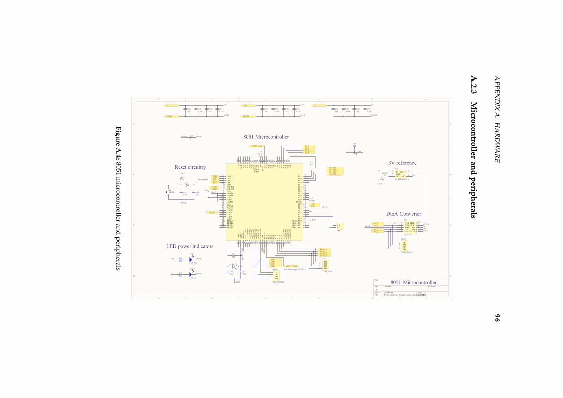
AP
PE
ND
IXA
.H
AR
DW
AR
E96
A.2
.3M
icroco
ntro
ller
an
dp
erip
he
rals
1
1
2
2
3
3
4
4
5
5
6
6
D D
C C
B B
A A
Title
Number RevisionSize
B
Date: 2007/09/20 Sheet of
File: C:\Documents and Settings\..\micro_processor.SchDocDrawn By:
12Y1
XTAL
C47
33pF
C46
33pF
R74
1M
En_1
Iref_1
FW_REV_1
En_2
Iref_2
FW_REV_2
En_3
Iref_3
FW_REV_3
En_4
Iref_4
FW_REV_4
Vdd
Vdd
Vdd
Vdd
DG
ND
DGND
DG
ND
Vaa
Vaa
AGND
Vaa Vdd
RX0TX0
Din
sel_DAC
sel_DAC
Din
SCLK
SCLK
5VDGND
DGNDDGND
AGNDAGND
5V5V
C40
1uF
C41
0.1uF
DGND
TMS
TCKTDITDO
JTAG PORT
R72
10k
Vdd
S1
SW-PB
SPD1SPD2SPD3SPD4
CANRXCANTX
R73
1k
C44
0.1uF
C45
1uF
R69
0
DGNDAGND
C42
1uF
C43
0.1uF
C36
1uF
C37
0.1uF
C38
1uF
C39
0.1uF
C32
1uF
C33
0.1uF
C34
1uF
C35
0.1uF
R70
120
LED1
LED yllw
Vdd DGND
R71
560
LED2
LED red
5V DGND
Tacho_1Tacho_2Tacho_3Tacho_4
RS232_valid
SYNC_PULSE
external interrupt /INT1 P2.7
Vdd
MO
NE
N
DGND
AGND
5VDGND
C67
0.1uF
DGND
N.C.N.C.
TP11
TP22
TP33
TP44
TPs1
TEST_POINT
TP11
TP22
TP33
TP44
TPs2
TEST_POINT
TP11
TP22
TP33
TP44
TPs3
TEST_POINT
VoA1
VoB2
GND3
VoC4
VoD5
SCLK6
Din7
Vdd8
/SYNC9
REFIN10
IC6
DAC7554
IN1
GND2
NC3
NC4
OUT5
IC14
3V_REFERENCE
TMS1
TCK2
TDI3
TDO4
/RST5
CANRX6
CANTX7
AV+8
AGND9
AGND10
AV+11
VREF12
AGND13
AV+14
VREFD15
VREF016
VREF217
AIN018
AIN119
AIN220
AIN321
HVCAP22
HVREF23
HVAIN+24
HVAIN-25
XT
AL
22
7
MO
NE
N2
8
AIN
1.7
/P1.
72
9
AIN
1.6
/P1.
63
0
AIN
1.5
/P1.
53
1
AIN
1.4
/P1.
43
2
AIN
1.3
/P1.
33
3
AIN
1.2
/P1.
23
4
AIN
1.1
/P1.
13
5
AIN
1.0
/P1.
03
6
Vdd
37
DG
ND
38
P2
.73
9
P2
.64
0
P2
.54
1
P2
.44
2
P2
.34
3
P2
.24
4
P2
.14
5
P2
.04
6
AIN
3.7
/P3.
74
7
AIN
3.6
/P3.
64
8
XT
AL
12
6
AIN
3.5
/P3.
54
9
AIN
3.4
/P3.
45
0
AIN3.3/P3.351
AIN3.2/P3.252
AIN3.1/P3.153
AIN3.0/P3.054
P0.755
P0.656
P0.557
P0.458
P0.359
P0.260
P0.161
P0.062
DGND63
Vdd64
P7.765
P7.666
P7.567
P7.468
P7.369
P7.270
P7.171
P7.072
P6.773
P6.674
P6.575
P6
.47
6P
6.3
77
P6
.27
8P
6.1
79
P6
.08
0P
5.7
81
P5
.68
2P
5.5
83
P5
.48
4P
5.3
85
P5
.28
6P
5.1
87
P5
.08
8D
GN
D8
9V
dd9
0/W
R/P
4.7
91
/RD
/P4.
69
2A
LE
/P4
.59
3P
4.4
94
P4
.39
5P
4.2
96
P4
.19
7P
4.0
98
DA
C1
99
DA
C0
100
IC58051
cur_5V
12
JP1
TP3
VDD
VDD
8051 Microcontroller
3V reference
DtoA Converter
8051 Microcontroller
Reset circuitry
LED power indicators
Fig
ure
A.4
:8
05
1m
icroco
ntro
llera
nd
perip
hera
ls

APPENDIX A. HARDWARE 97
A.3 Rate sensor PCB schematics
In this section the PCB schematics for the rate sensor system will be given.
The system is divided over four PCBs: The main rate sensor PCB and three
equivalent othogonally mounted rate sensor PCBs. The main PCB includes
the following components:
• Digital to analog converter
• 2 V reference supply component
• Power and I2C connectors
• Connectors for each of the three mounted PCBs
• Operational amplifiers to change the rate sensor output voltage levels
The rate sensors themselves are soldered onto the three equivalent orthogo-
nally mounted rate sensor PCBs. Each PCB has space for three rate sensors.
The other components on this PCB are the rate sensor peripheral components
including the passive analog first order filter.

AP
PE
ND
IXA
.H
AR
DW
AR
E98
A.3
.1R
ate
sen
sor
Ma
inP
CB
1
1
2
2
3
3
4
4
D D
C C
B B
A A
Title
Number RevisionSize
A4
Date: 2007/09/20 Sheet of File: C:\Documents and Settings\..\gyros.SchDocDrawn By:
-RG1
-IN2
+IN3
-VS4
Vref5
OUT6
+VS7
+RG8
IC4
AD623
-RG1
-IN2
+IN3
-VS4
Vref5
OUT6
+VS7
+RG8
IC5
AD623
-RG1
-IN2
+IN3
-VS4
Vref5
OUT6
+VS7
+RG8
IC6
AD623
-RG1
-IN2
+IN3
-VS4
Vref5
OUT6
+VS7
+RG8
IC8
AD623
-RG1
-IN2
+IN3
-VS4
Vref5
OUT6
+VS7
+RG8
IC9
AD623
-RG1
-IN2
+IN3
-VS4
Vref5
OUT6
+VS7
+RG8
IC10
AD623
-RG1
-IN2
+IN3
-VS4
Vref5
OUT6
+VS7
+RG8
IC11
AD623
-RG1
-IN2
+IN3
-VS4
Vref5
OUT6
+VS7
+RG8
IC3
AD623
-RG1
-IN2
+IN3
-VS4
Vref5
OUT6
+VS7
+RG8
IC7
AD623
Gout1_2
5V
AGND
Gout2_2
Gout3_2
Gout1_1
5VAGND
Gout2_1
Gout3_1
Gout1_3
5VAGND
Gout2_3
Gout3_3
R15
100K
R14
100K
R13
100K
R12
100K
R11
100K
R10
100K
R16
100K
R17
100K
R18
100K
2Vref
2Vref
2Vref
2Vref
2Vref
2Vref
2Vref
2Vref
2Vref
AGND
AGND
AGND
AGND
AGND
AGND
AGND
AGND
AGND
3V
3V
3V
3V
3V
3V
3V
3V
3V
AGND
AGND
AGND
AGND
AGND
AGND
AGND
AGND
AGND
AIN01
AIN12
AIN23
AIN34
AIN45
AIN56
AIN67
SCL9
SDA10
GND11
AIN78
Vdd12
AIN11/REF13
AIN1014
AIN915
AIN816
IC12
MAX1239
GtoA1_1
GtoA1_2
GtoA1_3
GtoA1_1
GtoA1_2GtoA1_3
GtoA2_1
GtoA2_2
GtoA2_3
GtoA2_1GtoA2_2GtoA2_3
GtoA3_1
GtoA3_2
GtoA3_3
GtoA3_1GtoA3_2
GtoA3_3
AGND3V
SDASCL
Gout1_1
Gout1_2
Gout1_3
Gout2_1
Gout2_2
Gout2_3
Gout3_1
Gout3_2
Gout3_3
5K6
R20Res35K6
R19Res3
5V
Gtemp1Gtemp2Gtemp3
Gtemp1
Gtemp2
Gtemp3
NC
NC
NC C110nF
C210nF
C3
10nF
C410nF
C510nF
C610nF
C710nF
C810nF
C9
10nF
5V3V
Power Connector
AGND
5V1
AGND2
Gout13
Gout24
Gout35
Gtemp6
Stest7
NC8
CON1
rate_sensor_con_Mboard
5V1
AGND2
Gout13
Gout24
Gout35
Gtemp6
Stest7
NC8
CON2
rate_sensor_con_Mboard
5V1
AGND2
Gout13
Gout24
Gout35
Gtemp6
Stest7
NC8
CON3
rate_sensor_con_Mboard
SCLSDA
5V1
3V2
GND3
SCL4
SDA5
STest6
JP2
POWER
STest
STest
STest
STest
R21
47K
5V
100nFC10
AGND
100nF
C11
AGND
100nFC12
AGND
100nFC13
AGND
100nF
C14
AGND
100nFC15
AGND
100nFC16
AGND
100nF
C17
AGND
100nF
C18
AGND
C1910nF
C2010nF
R2
25K5
R1
13K3
R323K7
3V
2Vref
3V
ADJ1
GND2
SHDN3
IN4
OUT5
IC1
MAX6037
DtoA converter
2V reference
Rate sensor Main PCB
AGND
AGND
AGND
AGND
AGND
AGND
AGND
AGND
AGND
AGND
Fig
ure
A.5
:M
ain
Ra
tesen
sor
PC
B

AP
PE
ND
IXA
.H
AR
DW
AR
E99
A.3
.2R
ate
sen
sor
Mo
un
ting
PC
B
1
1
2
2
3
3
4
4
D D
C C
B B
A A
Title
Number RevisionSize
A4
Date: 2007/09/20 Sheet of File: C:\Documents and Settings\..\gyro_board_small.SchDocDrawn By:
AGND Stest
Stest
AGND
AG
ND
5V NC
Gtemp
Gtemp1
AG
ND
AG
ND
Gout1Gout2 Gout3
Gout1
100nF
C4
Cap
100nF
C6
Cap
1uF
C5
Cap
5V
AGND PGND
100nF
C7
Cap
100nF
C9
Cap
1uF
C8
Cap
5V
AGND PGND
100nF
C1
Cap
100nF
C3
Cap
1uF
C2
Cap
5V
AGND PGND
PG
ND
PG
ND
PG
ND
R1
0R
PGND AGND
25V
C10
22nF
25VC1122nF
25VC161uF
AGND
PG
ND
6G
PG
ND
7F
AG
ND
1F
AG
ND
2G
AV
cc3A
AV
cc3B
Pdd
6E
Pdd
7E
ST15F
ST15G
ST24F
ST24G
CP15A
CP15B
CP24A
CP24B
CP36C
CP37C
CP46A
CP47B
CP56D
CP57D
SUMJ1C
SUMJ2C
RateOut1B
RateOut2A
Cmid1D
Cmid2D
Vref1E
Vref2E
TEMP3F
TEMP3G
IC2Rate Sensor
PG
ND
6G
PG
ND
7F
AG
ND
1F
AG
ND
2G
AV
cc3A
AV
cc3B
Pdd
6E
Pdd
7E
ST15F
ST15G
ST24F
ST24G
CP15A
CP15B
CP24A
CP24B
CP36C
CP37C
CP46A
CP47B
CP56D
CP57D
SUMJ1C
SUMJ2C
RateOut1B
RateOut2A
Cmid1D
Cmid2D
Vref1E
Vref2E
TEMP3F
TEMP3G
IC3Rate Sensor
PG
ND
6G
PG
ND
7F
AG
ND
1F
AG
ND
2G
AV
cc3A
AV
cc3B
Pdd
6E
Pdd
7E
ST15F
ST15G
ST24F
ST24G
CP15A
CP15B
CP24A
CP24B
CP36C
CP37C
CP46A
CP47B
CP56D
CP57D
SUMJ1C
SUMJ2C
RateOut1B
RateOut2A
Cmid1D
Cmid2D
Vref1E
Vref2E
TEMP3F
TEMP3G
IC1Rate Sensor
Stest
AGND
25V
C12
22nF
25VC1322nF
25VC171uF
AGND
Stest
AGND
25V
C14
22nF
25VC1522nF
20V
C181uF
AGND
C19
39nF
C22
100nF
AGNDNCNC
Gtemp2
Gout2
C20
39nF
C23
100nF
AGNDNCNC
Gtemp3
Gout3
C21
39nF
C24
100nF
AGNDNCNC
5V1
AGND2
Gout13
Gout24
Gout35
Gtemp6
Stest7
NC8
CON1
rate_sensor_con_Sboard
11
22
33
44
55
66
JP1
Jumper2X3
Gtemp1Gtemp2Gtemp3
Gtemp
Connector to main PCB Temp output select
Rate Sensor 1 Rate Sensor 2 Rate Sensor 3
Rate Sensor mount PCB
Fig
ure
A.6
:R
ate
senso
rP
CB
-m
ou
nted
toth
estru
cture

APPENDIX A. HARDWARE 100
A.4 Rate sensor filter design
Equation (A.4.1) was used to calculate the resistor and capacitor values for
the passive first order low pass filter. Seeing that a 180 KΩ resistor is inte-
grated into the rate sensor package, only the value of the capacitor needed
to be determined. The required filter 3 dB cut off frequency is 20 Hz, as dis-
cussed in section 4.3.1. According to equation (A.4.1) a 44 nF capacitor is
required for the specified cut off frequency. A 39 nF capacitor was therefore
used, which results in a cut off frequency of 22.7 Hz. Figure A.7 shows the 3
dB cut off frequency of 22.7 Hz (or 142.6 rad/s) on a bode plot of the passive
first order low pass filter.
f3dB =1
2πRC(A.4.1)
−20
−15
−10
−5
0
Mag
nitu
de (
dB)
101
102
103
−90
−45
0
Pha
se (
deg)
Bode Diagram
Frequency (rad/sec)
Figure A.7: Rate sensor Filter - Bode Plot

Appendix B
BLDC motors datasheets
The three BLDC motors as shown in Figure B.2, B.3 and B.4 were compared
to determine which would fit the application best. Equation (B.0.1) was used
to calculate the power usage of each of the three BLDC motors at the speci-
fied maximum output torque of 5 mNm and the specified maximum angular
velocity of 5000 rpm. The equation for a DC motor was used for this calcu-
lation, but the power consumption of a BLDC motor can be calculated using
the same equation. The results of the power calculations are shown in Ta-
ble B.1. The meaning of the variables in equation (B.0.1) is depicted by the
schematic in Figure B.1.
Figure B.1: Schematic to describe a DC motor
101

APPENDIX B. BLDC MOTORS DATASHEETS 102
Pmax = Va max Ia max
= (VRa max + E0 max) Ia max (B.0.1)
Where,
Va max = Maximum voltage over armature
Ia max = Nmax/Nconst + INL
= Maximum armature current
INL = No load current
Nconst = Torque constant
Nmax = 5 mNm
= Maximum torque specification
VRa max = Ia max Ωterminal
= Maximum voltage over armature resistance
Ωterminal = Terminal resistance
E0 max = ωmax/ωconst
= Maximum back EMF
ωconst = Speed constant
ωmax = 5000 rpm
= Maximum rotational speed specification

APPENDIX B. BLDC MOTORS DATASHEETS 103
Table B.1: Power consumption of the BLDC motors compared
Motor Data Maxon 6 W Faulhaber Maxon 15 W
Nconst:Torque Constant [mNm/A] 9.5 6.34 49
INL:No load current [mA] 110 102 73
Ia:Armature current [mA] 636 891 175
ωconst:Speed Constant [rpm/V] 1007 1506 195
Ωterminal:Terminal resistance [Ohm] 4.5 3.4 13.7
VRa:Armature voltage [V] 2.86 3.03 2.4
E0 [V]: 4.97 3.32 25.64
Power Consumption [W]: 4.98 5.65 4.92

APPENDIX B. BLDC MOTORS DATASHEETS 104
Figure B.2: Maxon EC flat BLDC motor: 6W

APPENDIX B. BLDC MOTORS DATASHEETS 105
Figure B.3: Faulhaber BLDC motor
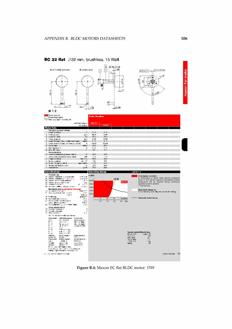
APPENDIX B. BLDC MOTORS DATASHEETS 106
Figure B.4: Maxon EC flat BLDC motor: 15W

Appendix C
Rate sensor verification results
The test results which were used to verify the results shown in section 6.5 will
be given in this section. Two test results sets were used to verify the results
in section 6.5. They will be referred to as rate sensor result set 2 and 3 in this
section. It can be seen that the variance of the data in result set 1 is larger
that the variance in result set 2. This is due to the fact that the temperature
variations during the recording of the data in result set 2 was larger than
the temperature variations in result set 3. Both result sets 2 and 3 verify the
results in section 6.5 successfully.
C.0.1 Rate sensor result set 2
The covariance matrix of the rate sensor outputs (of result set 2) is shown in
equation (C.0.1) (with units of 1 × 10⁻⁵ rad2/s2).
R =
0.806 −0.017 −0.003 0.001 0.002 −0.014
−0.017 1.165 0.005 −0.013 0.011 0.044
−0.003 0.005 0.885 −0.004 0.003 0.008
0.001 −0.013 −0.004 2.674 −0.001 −0.011
0.002 0.011 0.003 −0.001 0.766 0.007
−0.014 0.044 0.008 −0.011 0.007 1.029
(C.0.1)
The covariance matrix of the derivative taken of the filtered rate sensor out-
puts of result set 2 (with units of 1 × 10⁻¹¹ rad2/s4) is shown in equation
(C.0.2).
107

APPENDIX C. RATE SENSOR VERIFICATION RESULTS 108
Figure C.1: Rate Sensor outputs over 2 hours (Result set 2)
100
101
102
103
10−4
T[s]
Alla
n D
evia
tion
Allan Variance vs decimation ratio
100
101
102
103
104
10−4
T[s]
Alla
n D
evia
tion
Allan Variance vs decimation ratio
100
102
101
103
10−4
T[s]
Alla
n D
evia
tion
Allan Variance vs decimation ratio
100
101
102
103
10−4
T[s]
Alla
n D
evia
tion
Allan Variance vs decimation ratio
100
101
102
103
10−4
T[s]
Alla
n D
evia
tion
Allan Variance vs decimation ratio
100
101
102
103
10−4
T[s]
Alla
n D
evia
tion
Allan Variance vs decimation ratio
Figure C.2: Allan Variance of the rate sensor outputs (Result set 2)
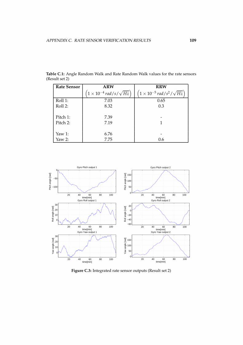
APPENDIX C. RATE SENSOR VERIFICATION RESULTS 109
Table C.1: Angle Random Walk and Rate Random Walk values for the rate sensors(Result set 2)
Rate Sensor ARW RRW(
1 × 10⁻⁴ rad/s/√
Hz) (
1 × 10⁻⁵ rad/s2/√
Hz)
Roll 1: 7.03 0.65Roll 2: 8.32 0.3
Pitch 1: 7.39 -Pitch 2: 7.19 1
Yaw 1: 6.76 -Yaw 2: 7.75 0.6
20 40 60 80 100
−100
−50
0
time[min]
Pitc
h an
gle
[rad
]
Gyro Pitch output 1
20 40 60 80 1000
50
100
150
time[min]
Pitc
h an
gle
[rad
]
Gyro Pitch output 2
20 40 60 80 100
0
10
20
30
time[min]
Rol
l ang
le [r
ad]
Gyro Roll output 1
20 40 60 80 100−60
−40
−20
0
20
time[min]
Rol
l ang
le [r
ad]
Gyro Roll output 2
20 40 60 80 100
0
10
20
30
time[min]
Yaw
ang
le [r
ad]
Gyro Yaw output 1
20 40 60 80 1000
50
100
150
time[min]
Yaw
ang
le [r
ad]
Gyro Yaw output 2
Figure C.3: Integrated rate sensor outputs (Result set 2)

APPENDIX C. RATE SENSOR VERIFICATION RESULTS 110
20 40 60 80 100
−1
−0.5
0
0.5
1
x 10−3
time[min]
Pitc
h ra
te [r
ad/s
]
Gyro Pitch output 1
20 40 60 80 100
−1
0
1
x 10−3
time[min]
Pitc
h ra
te [r
ad/s
]
Gyro Pitch output 2
20 40 60 80 100−10
−5
0
5
x 10−4
time[min]
Rol
l rat
e [r
ad/s
]
Gyro Roll output 1
20 40 60 80 100
−5
0
5
10
x 10−4
time[min]
Rol
l rat
e [r
ad/s
]
Gyro Roll output 2
20 40 60 80 100
−5
0
5
x 10−4
time[min]
Yaw
rat
e [r
ad/s
]
Gyro Yaw output 1
20 40 60 80 100
−1
0
1
x 10−3
time[min]
Yaw
rat
e [r
ad/s
]
Gyro Yaw output 2
Figure C.4: Filtered rate sensor outputs - cut off frequency 0.01 Hz (Result set 2)
Figure C.5: Temperature outputs of rate sensors (Result set 2)
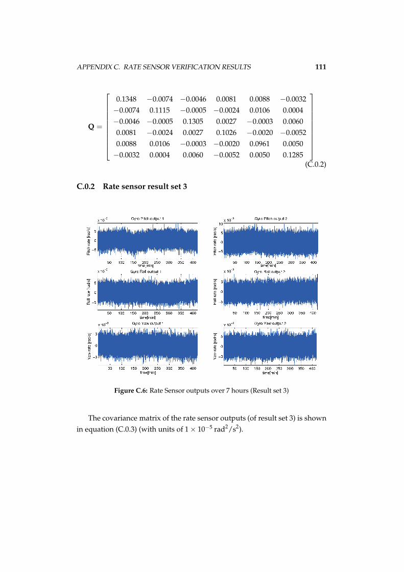
APPENDIX C. RATE SENSOR VERIFICATION RESULTS 111
Q =
0.1348 −0.0074 −0.0046 0.0081 0.0088 −0.0032
−0.0074 0.1115 −0.0005 −0.0024 0.0106 0.0004
−0.0046 −0.0005 0.1305 0.0027 −0.0003 0.0060
0.0081 −0.0024 0.0027 0.1026 −0.0020 −0.0052
0.0088 0.0106 −0.0003 −0.0020 0.0961 0.0050
−0.0032 0.0004 0.0060 −0.0052 0.0050 0.1285
(C.0.2)
C.0.2 Rate sensor result set 3
Figure C.6: Rate Sensor outputs over 7 hours (Result set 3)
The covariance matrix of the rate sensor outputs (of result set 3) is shown
in equation (C.0.3) (with units of 1 × 10⁻⁵ rad2/s2).

APPENDIX C. RATE SENSOR VERIFICATION RESULTS 112
100
102
101
103
10−3.9
10−3.2
T[s]
Alla
n D
evia
tion
Allan Variance vs decimation ratio
100
102
101
103
10−3.9
10−3.5
10−3.1
T[s]
Alla
n D
evia
tion
Allan Variance vs decimation ratio
100
102
101
103
10−3.9
10−3.2
T[s]
Alla
n D
evia
tion
Allan Variance vs decimation ratio
100
102
101
10−3.9
10−3.2
T[s]
Alla
n D
evia
tion
Allan Variance vs decimation ratio
100
102
101
103
10−3.9
10−3.2
T[s]
Alla
n D
evia
tion
Allan Variance vs decimation ratio
100
102
101
103
10−3.9
10−3.5
10−3.1
T[s]
Alla
n D
evia
tion
Allan Variance vs decimation ratio
Figure C.7: Allan Variance of the rate sensor outputs (Result set 3)
Table C.2: Angle Random Walk and Rate Random Walk values for the rate sensors(Result set 3)
Rate Sensor ARW RRW(
1 × 10⁻⁴ rad/s/√
Hz) (
1 × 10⁻⁵ rad/s2/√
Hz)
Roll 1: 7.07 1.8Roll 2: 8.36 1
Pitch 1: 7.35 0.8Pitch 2: 7.29 -
Yaw 1: 6.79 0.85Yaw 2: 7.8 1

APPENDIX C. RATE SENSOR VERIFICATION RESULTS 113
50 100 150 200 250 300 350 400−30
−20
−10
0
10
time[min]
Pitc
h an
gle
[rad
]
Gyro Pitch output 1
50 100 150 200 250 300 350 400
0
10
20
30
time[min]
Pitc
h an
gle
[rad
]
Gyro Pitch output 2
50 100 150 200 250 300 350 400
−10
0
10
time[min]
Rol
l ang
le [r
ad]
Gyro Roll output 1
50 100 150 200 250 300 350 400
−20
−10
0
time[min]
Rol
l ang
le [r
ad]
Gyro Roll output 2
50 100 150 200 250 300 350 4000
10
20
30
time[min]
Yaw
ang
le [r
ad]
Gyro Yaw output 1
50 100 150 200 250 300 350 400
−10
−5
0
5
time[min]
Yaw
ang
le [r
ad]
Gyro Yaw output 2
Figure C.8: Integrated rate sensor outputs (Result set 3)
50 100 150 200 250 300 350 400−2
−1
0
1x 10
−3
time[min]
Pitc
h ra
te [r
ad/s
]
Gyro Pitch output 1
50 100 150 200 250 300 350 400
−5
0
5
10
x 10−4
time[min]
Pitc
h ra
te [r
ad/s
]
Gyro Pitch output 2
50 100 150 200 250 300 350 400
−5
0
5
10x 10
−4
time[min]
Rol
l rat
e [r
ad/s
]
Gyro Roll output 1
50 100 150 200 250 300 350 400
−5
0
5
x 10−4
time[min]
Rol
l rat
e [r
ad/s
]
Gyro Roll output 2
50 100 150 200 250 300 350 400
−5
0
5
10x 10
−4
time[min]
Yaw
rat
e [r
ad/s
]
Gyro Yaw output 1
50 100 150 200 250 300 350 400
−5
0
5
10x 10
−4
time[min]
Yaw
rat
e [r
ad/s
]
Gyro Yaw output 2
Figure C.9: Filtered rate sensor outputs - cut off frequency 0.002 Hz (Result set 3)

APPENDIX C. RATE SENSOR VERIFICATION RESULTS 114
Figure C.10: Temperature outputs of rate sensors (Result set 3)
R =
0.4006 −0.0116 −0.0063 0.0024 −0.0135 0.0036
−0.0116 0.5476 −0.0011 −0.0016 0.0032 −0.0028
−0.0063 −0.0011 0.4223 0.0011 0.0000 0.0014
0.0024 −0.0016 0.0011 0.4006 −0.0069 0.0020
−0.0135 0.0032 0.0000 −0.0069 0.3556 −0.0016
0.0036 −0.0028 0.0014 0.0020 −0.0016 0.4655
(C.0.3)
The covariance matrix of the derivative taken of the filtered rate sensor out-
puts of result set 3 (with units of 1 × 10⁻¹¹ rad2/s4) is shown in equation
(C.0.4).
Q =
0.4088 −0.0096 0.0019 −0.0044 −0.0369 0.0105
−0.0096 0.2820 0.0287 0.0069 0.0119 −0.0043
0.0019 0.0287 0.3434 −0.0065 0.0299 0.0275
−0.0044 0.0069 −0.0065 0.3209 −0.0036 −0.0120
−0.0369 0.0119 0.0299 −0.0036 0.2563 −0.0516
0.0105 −0.0043 0.0275 −0.0120 −0.0156 0.4093
(C.0.4)

Appendix D
Moment of inertia
determination method
This chapter explaines the string suspension method used to determination
the moment of inertia of each reaction wheel rotor, as explained by Peddle
[11]. The representation of the setup is given in Figure D.1. Equation (D.0.1)
shows the formula for the moment of inertia determination. Table D.1 shows
the measured periods of oscillation after the setup was given an initial offset
position.
Figure D.1: The string suspension method for moment of inertia determination
115

APPENDIX D. MOMENT OF INERTIA DETERMINATION METHOD 116
Table D.1: Periods of oscillation measured for the reaction wheel rotor
Measured values for 10 periods of oscillation:
τ [s] 20.77 21.65 21.19 21.52 21.77 21.92 20.99 22 21.66 21.78
Mean period of oscillation [s] : 2.15 s
I =mgr2
4π2lτ2 (D.0.1)
Where,
I = 47.08 × 10−6
= Moment of inertia of the rotor
m = 85.19 g
= Mass of each rotor
g = 9.81 m/s2
= Gravitational acceleration
r = 25 mm
= Radius of the rotor
l = 1.2 m
= Length of the suspension string
τ = 2.15 s
= Period of oscillation (see Table D.1)
constraint:
l ≫ r

Bibliography
[1] Baker, E.A. 2006. The Design of a CMOS Sensor Camera for Space
Applications. Thesis (MScEng). University of Stellenbosch.
[2] Bayard, D.S. et al. 2005. High Accuracy Inertial Sensors from
Inexpensive Components. United States Patent. California
Institute of Technology.
[3] Bijker, J. 2006. Development of an Attitude Heading Reference
System for an Airship. Thesis (MScEng). University of
Stellenbosch.
[4] Bootsma, R. 1997. Kragstelselondersoek vir die Sunsat
Mikrosatelliet. Thesis (MScEng). University of Stellenbosch.
[5] Chen, X., Steyn, W.H., Hashida, Y. 2000. Ground-Target
Tracking Control of Earth-Pointing Satellites. AAIA Guidance,
Navigation and Control Conference and Exhibit. Surrey
Space Centre, University of Surrey, Guildford, UK.
[6] Cropp, A., Collingwood, C. 2006. The Characterization and
Testing of MEMS Gyros for GIOVE-A. AAIA Guidance,
Navigation and Control Conference and Exhibit. Surrey
Satellite Technology Ltd, Guildford, UK.
[7] Dussy, S., Durrant, D., Moy, T. 2005. MEMS gyro for space
applications Overview of European activities. AAIA Guidance,
Navigation and Control Conference and Exhibit. August
2005, San Francisco, California, USA.
117

BIBLIOGRAPHY 118
[8] Greyling, B.C. 1995. A Charge Coupled Device Star Sensor
System for a Low Earth Orbit Microsatellite. Thesis (MScEng).
University of Stellenbosch.
[9] Hou, H. 2004. Modeling Inertial Sensor Errors Using Allan
Variance. Thesis (MScEng). University of Calgary.
[10] Ntsimane, M.H. 2001. The Attitude Determination and Control
Systems Task Scheduler. Thesis (MScEng). University of
Stellenbosch.
[11] Peddle, I.K. 2005. Autonomous flight of a model aircraft. Thesis
(MScEng). University of Stellenbosch.
[12] Prezzavento, A.M. 2002. 3-Axis Micro Gyroscope Feasibility
Study. Final Report. Astrium LTD, Stevenage, Herts, England.
[13] Sidi, M.J. 2000. Spacecraft dynamics and control : a practical
engineering approach. Cambridge University Press.
[14] Stockwell, W. 2003. Angle Random Walk. Application note.
Crossbow Technology Inc.
[15] Stockwell, W. 2003. Bias Stability Measurement: Allan Variance.
Application note. Crossbow Technology Inc.
[16] Wertz, J.R. 1999. Space Mission Analysis and Design. Space
Technology Library.
[17] Steyn, W.H. 1995. A Multi-mode Attitude Determination and
Control System for Small Satellites. Thesis (PhDEng).
University of Stellenbosch.
[18] Wie, B., Weiss, H., Arapostathis, A. 1989. Quaternion Feedback
Regulator for Spacecraft Eigenaxis Rotations. Journal of
Guidance Control and Dynamics, Vol. 12, May-June 1989, pp.
375-379, University of Texas at Austin, Austin, Texas, USA.
[19] Wie, B., Bailey, D., Heiberg, C. 2002. Rapid Multitarget
Acquisition and Pointing Control of Agile Spacecraft. Journal of
Guidance Control and Dynamics, Vol. 25, January-February

BIBLIOGRAPHY 119
2002, pp. 96-104, Arizona State University, Tempe, Arizona,
USA.