attention: professor bart selman department of computer science
TRANSCRIPT

Attention: Professor Bart Selman
Department of Computer Science
Raphael Rubin
MENG ECE Cornell University
Statistical Arbitrage between same sector securities, Semester II, 2006-2007
Table of Contents:
Executive Summary
I. Methodology…………………………………………………………………………………p142
II. Computation of Coeeficients of the LM Matrix……………………………………………..p146
III. Code Reference……………………………………………………………………………....
.p154

Executive Summary:
This is an attempt to put to the disposition of the public the application of the theory behind Neural Networks General Hetero Scedascticity models.
Its purpose is to model the discrepancies observed beween two same sector stocks whose short term behavior should be equivalent, due to heteroscedasticity, meaning the influence of a past chock on the future performance of a stock.
Exploiting these arbitrages might provide incentives for day traders to short and buy stocks.
We have written an application which applies most of the theory behind NN and Garch Models and in particular: Financial statistical modelling with a new nature-inspired technique Nikos S. Thomaidis_1, George D. Dounias1, and Nick Kondakis1,2.
However, we would have required more time to complete this work.
It is therefore an attempt which should be continued and developed so as to provide efficient information to the public of investors.
Second n: 22Mean: 26.765

Sigma: 30.905560071503853Beta1: 44.56499995729246Beta2: 0.5000000016332251unit root not detected in regular regressionunit root not detected in improved regression
I. Methodology:
We record share price every 10 seconds, along best bid and offer. We analyze the French stock market index CAC 40.
The market trades from 9:00 to 17:30
1) We parse the real-time (approximately) data to get the desired information.
2) We store it into the database under
OPEN HIGH LOW CURRENT CLOSE PRICE SPURRIOUS
2-a) We check for price inconsistencies:
2-b) check for highest
2-c) check for lowest
2-c) check for closing price
2-d) check for opening price
3) We run a filtering algorithm to remove spurious trades from the data.
1-minute bars include the open high low and close price

Extract from ‘calcul stochastique’ regarding normalization of the sampled data into non explosive trajectory.
4) We run a linear regression of the two stocks (here Accor and Adecco).
5) neural network-GARCH models:
A typical ARMA(r,s)GARCH(p,q) takes the form
etzteyiyts
iti
r
iti 11
q
iti
p
iti ebihaiaht1
2
10
Ht represents the variance of the conditionally heteroskedastic normal process et.
To ensure positivity and non explosive behavior of ht, the following conditions must be met:

1
0,
00
ii
ii
6) LM test for GARCH effects:
The difficulty of testing for a GARCH process is that the LM test statistic for the ARCH(q) null Ho is the same whether the alternative is ARCH(q+r) or GARCH(r,q).
),(..........:2
)(......:
)(......:
21
210
21
210
2
221
210
21
21
210
2
qrGARCHH
rqARCHH
qARCHHo
qtqtqtqtt
rqtrqqtqtt
qtqtt
For the ARCH(q), the null hypothesis amounts to all alpha’s to be null; against the hypothesis that at least one the alpha i=1,q be not null.
Under the null, OLS is consistent, whereas under the alternative(lagged variables), autocorrelation and heteroscedasticity induce inefficiency.
The LM test in our case starts by a linear model and under the assumption of homoscedastic errors uses Ordinary Least Squares to estimate the regression equation:
etxiytn
tii 1
,
Against the hypothesis
))1(1(*11
,1
, cxwigammaFlambdaxiytn
ntn
n
tii
As achieved by our program application, we compute the OLS residuals.

We may compute at a level of significance alpha%, the t-student of the estimated coeeficients.
However, we will preferably compute the Fisher_Snedecor statistics for the ensemble of the estimators joint effect following the procedure as described p129,p183 Econometrie, Jean-Pierre Berdot; whereas t-student statistics is focused on individual coefficients significance..
To assess, whether the coefficients are significant, whether these exogenous variables exerce an effect on the endogenous variable y, we test the linear hypothesis against one neuron, that is the linear subset(n coefficients) against the full set (2 n coeeficients).
II. Computation of coefficients:
1- In order to assess coefficients under the exponential we must operate a transformation.
6/)125.025.0(125.1)1/(1
:
)1()1(2''
)1('
6/)0)(0(''2/)0).(0(')0()1/(1
2
223
2
2
zze
Therefore
eeeef
eef
zzzfzzzfzfe
z
zzzz
zz
z
After having made the null assessment for a linear versus a one nurone model, we test one neuron against a two neuron for half the significance interval.
At each subsequent test, we half the significance level.
We may use the F test of Wald, or the Vraisemblance ratio or the TR2.
2-
Next, we compute the LM statistics testing the null hypothesis of no ARCH against ARCH of a given order:
We test for ARCH errors:
We regress 2et on a constant and the other 2
1et , 2
qet , ..and if the null is rejected, carry on; We
do another test for different values of q.

Confidence intervals and tests of significance are available from the log-likelihood function. The (pxp) matrix of second partial derivatives of the log-likelihood function taken with respect to the parameters is called the
"Hessian" matrix. The inverse of (-1)*(The Hessian matrix) is the asymptotic covariance matrix of the parameter estimates. The square roots of the diagonal elements of the asymptotic covariance matrix are the asymptotic standard errors of the parameter estimates, and these are used for intervals and tests in the usual way, except with standard normal critical values instead of critical values from the t distribution.
We get the standard errors looking at the inverse of diagonal values, and obtain also the covariance between them.

tcztAcxwigammaFlambdaxiytn
ntn
n
tii ),())1(1(*11
,1
,
),(1
2
10 vztBebihaiaht
q
iti
p
iti
A( ) and B( ) are assumed continuous and twice differentiable for all vc ,
We assume as in the article that ),( cztA and ),( vztB are 0 for vc , =0.
Therefore the null hypothesis is that vc , =0.
The classical LMT takes the form:
0..TheQMLE follows the law N~(0,C) where C is the variance-auto-covariance matrix.
As found in the annex,
A=
'''
'''
'''
AAA
AAA
AAA
C= 11 IAA
A has been computed using A= )(*/1 htET
Whereas WE= )''(*/1 thET where h’’ is the product of simple derivatives instead of the
gradient.

3-
We estimate a GARCH(1,1) model using residuals of the conditional mean.
See for illustration: Engle’s Model of U.K. Inflation
a) Estimate using OLS the parameters 110 ,, , indeed, we know ht, the variance of et
from the OLS estimatorsb) Next, we make a joint estimation of the parameters of the GARCH(1,1) NN model.
(we use p275, J-P Berdot Econometrie)
6/)125.025.0(125.1)1/(1 2zze z
etcjxwigammacjxwigammalambdaxiytn
ntnj
n
ntnj
h
jj
n
tii
))6/)(125.0)(125.1(* 2
1,
1,
11,
AND
q
iti
p
iti ebihaiaht1
2
10
In a typical simultaneous equations model, we have n endogenous variables Y and m exogenous variables X.
In our case, yt and ht are endogenous, while xt and et are exogenous.
We need to translate the structural form into a reduced form where the endogenous are expressedin function of the exogenous, in order to avoid simultaneity bias.
...))1(1...2.10(*10
)1(1...2.101
)(...1.10
ietFphtaphtaaaaht
ietFphtaphtaaht
ietFphtaphtaaht

Write this form for p=1,2.3 MAX.
We would omit insignificant parameters and re-estimate the model.
4-
We perform in-sample diagnostic tests: if the model passes all tests, accept it; otherwise complicate the mean and variance structure.
Misspecification tests:
All tests are built using the additive extension to our classical NN model.
H0 is that: 0, vc
Test for serial correlation (in the mean):
To test the null hypothesis of no serial dependence in the conditional mean we state the alternative as remaining autocorrelation of order rc in the ordinary residual process, i.e. A(zt; πc) = π′c*zt with zt = (εt−1, εt−2, ..., εt−rc ). The null hypothesis of no remaining serial dependence is thus equivalent to testing πc = 0. Under this null, the LM statistic is asymptotically χ2-distributed with rc degrees of freedom.
Here the J’s are still the second order derivative of the log-likelihood; we included the computation implemented in Java code in the annex.

We require
vvJ
ccJ
cJ
vl
cl
''
''
'
/
/
We also need to compute here again the information matrix I, product of single derivatives.
Test for neglected nonlinearity:
Test for neglected heteroskedasticity:
Normality tests: Jacques Bera statistics amongst others:
These tests are performed at every step of identification for every model.
http://www.uoguelph.ca/~tstengos/Nortest.pdf

III. Code Reference
/* Class Matrix
*

* Defines a matrix and includes the methods
* needed for standard matrix manipulations, e.g. multiplation,
* and related procedures, e.g. solution of linear
* simultaneous equations
*
* See class ComplexMatrix for complex matrix arithmetic
*
* WRITTEN BY: Dr Michael Thomas Flanagan
/*
package com.jrefinery.chart.demo;
import java.awt.*;
import java.awt.event.ActionEvent;
import java.awt.event.ActionListener;
import java.awt.event.WindowAdapter;
import java.awt.event.WindowEvent;
import java.util.Arrays;
import java.util.Random;
import java.util.Vector;
import java.io.BufferedReader;
import java.io.FileNotFoundException;
import java.io.FileReader;
import java.io.IOException;
import java.io.Reader;
import java.io.StreamTokenizer;
import javax.swing.JFrame;
import java.lang.Math;
import javax.swing.JPanel;
import javax.swing.Timer;
import org.jfree.chart.ChartPanel;
import org.jfree.chart.JFreeChart;
import org.jfree.chart.axis.DateAxis;
import org.jfree.chart.axis.NumberAxis;
import org.jfree.chart.plot.*;
import org.jfree.chart.renderer.*;
import org.jfree.chart.renderer.xy.StandardXYItemRenderer;
import org.jfree.chart.renderer.xy.XYItemRenderer;
import org.jfree.chart.renderer.xy.XYLine3DRenderer;
import org.jfree.data.time.*;
import org.jfree.chart.renderer.xy.XYItemRendererState;
import java.util.Random.*;
import java.lang.Math;
import java.util.*;
import org.jfree.*;
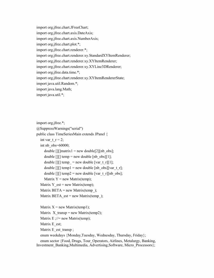
@SuppressWarnings("serial")
public class TimeSeriesMain extends JPanel {
int var_t_r = 2;
int nb_obs=60000;
double [][]matrix1 = new double[2][nb_obs];
double [][] temp = new double [nb_obs][1];
double [][] temp_ = new double [var_t_r][1];
double [][] temp1 = new double [nb_obs][var_t_r];
double [][] temp2 = new double [var_t_r][nb_obs];
Matrix Y = new Matrix(temp);
Matrix Y_est = new Matrix(temp);
Matrix BETA = new Matrix(temp_);
Matrix BETA_est = new Matrix(temp_);
Matrix X = new Matrix(temp1);
Matrix X_transp = new Matrix(temp2);
Matrix E ;//= new Matrix(temp);
Matrix E_est;
Matrix E_est_transp ;
enum weekdays {Monday,Tuesday, Wednesday, Thursday, Friday};
enum sector {Food, Drugs, Tour_Operators, Airlines, Metalurgy, Banking, Investment_Banking,Multimedia, Advertising,Software, Micro_Processors};

double sigma_est;
Information about a stock :
public class information {
String share_name;
String market_place;
Number opening_trading_time;
Number closing_trading_time;
double volatility;
double price;
double day_highest;
double day_lowest;
double month_lowest;
double month_highest;
}
The Synthetic assets are the assets tested with neural networks parameters for conditional heterscedasticity and whch should show in such hypothesis a unit root.
information Accor = new information();
information Adecco = new information();
information Synthetic = new information();
information Synthetic_improved = new information();
//store all these values into an array
private int line_number=0;
private double value1 = 0;
private double value2 = 0;
private TimeSeries total;
private TimeSeries free;
private TimeSeries synthetic;
private TimeSeries synthetic_improved;
final XYItemRenderer renderer1 = new StandardXYItemRenderer();
Reader r;
StreamTokenizer stok_number;

public TimeSeriesCollection dataset;
public TimeSeriesMain() {
super(new BorderLayout());
// create two series that automatically discard data more than 30 seconds old...
this.total = new TimeSeries("Accor", Second.class);
//30600 per day, taking an observation per second
this.total.setMaximumItemCount(nb_obs); //20 days or 612000 for 20 days
this.free = new TimeSeries("Addecco", Second.class);
this.free.setMaximumItemCount(nb_obs);
this.synthetic = new TimeSeries("Synthetic", Second.class);
this.synthetic.setMaximumItemCount(nb_obs);
this.synthetic_improved = new TimeSeries("Synthetic_Improved", Second.class);
this.synthetic_improved.setMaximumItemCount(nb_obs);
dataset = new TimeSeriesCollection();
dataset.addSeries(total);
dataset.addSeries(free);
dataset.addSeries(synthetic);
dataset.addSeries(synthetic_improved);
DateAxis domain = new DateAxis("Time");
NumberAxis range = new NumberAxis("Share Price");
XYPlot plot = new XYPlot(dataset, domain, range, renderer1);
plot.setBackgroundPaint(Color.white);
renderer1.setSeriesPaint(0, Color.red);
renderer1.setSeriesPaint(0, Color.BLUE);
renderer1.setSeriesPaint(0, Color.green);
renderer1.setSeriesPaint(0, Color.yellow);
renderer1.setStroke(
new BasicStroke(2f, BasicStroke.CAP_BUTT, BasicStroke.JOIN_BEVEL)
);

domain.setAutoRange(true);
domain.setLowerMargin(0.0);
domain.setUpperMargin(0.0);
domain.setTickLabelsVisible(true);
range.setStandardTickUnits(NumberAxis.createIntegerTickUnits());
JFreeChart chart = new JFreeChart(
"Share Price",
JFreeChart.DEFAULT_TITLE_FONT,
plot,
true
);
ChartPanel chartPanel = new ChartPanel(chart);
add(chartPanel);
}
private void addTotalObservation(double y) {
//read content of file
double Number;
try {
readfile("stocks_analytics.txt");
This file is built up by the Perl script, arbitrage trading below, extracting stocks information from boursorama.com
} catch (IOException e) {
// TODO Auto-generated catch block
e.printStackTrace();
}
//System.out.println("Total: \n"+matrix1[0][total.getItemCount()]);
}
private double readfile(String filename) throws IOException {

// TODO Auto-generated method stub
String sharename = "";
if(line_number==0){
r = new BufferedReader(new FileReader(filename));
stok_number = new StreamTokenizer(r);
}
//strings need to be quoted to be recgnized
line_number+=1;
while(stok_number.nextToken() != StreamTokenizer.TT_EOF) {
if (line_number % 2 == 0 && line_number >0)
return line_number;
We only parse two lines at a time(two stocks only, Accor and Adecco)
else{
switch(stok_number.ttype) {
case StreamTokenizer.TT_EOL:
line_number+=1;
break;
case StreamTokenizer.TT_NUMBER:
if(sharename.equals("Adecco")){
value1 = stok_number.nval;
this.Adecco.price=value1;
if(this.Adecco.day_lowest == 0)this.Adecco.day_lowest=this.Adecco.price;
total.addOrUpdate(new Second(), 8*(value1-this.Adecco.day_lowest));
Here we normalize by Adeccos’ lowest share price so as to visualize only relevant variation.
matrix1[0][total.getItemCount()] = value1;
X.setElement(total.getItemCount()-1, 0, 1);
X.setElement(total.getItemCount()-1, 1, value1);
line_number+=1;}
if(sharename.equals("Accor")){
value2 = stok_number.nval;
this.Accor.price=value2;
if(this.Accor.day_lowest == 0)this.Accor.day_lowest=this.Accor.price;

Second sec_instance = new Second();
free.addOrUpdate(sec_instance, 8*(value2-this.Accor.day_lowest));
System.out.println("Second n: \n"+sec_instance.getSecond());
matrix1[1][free.getItemCount()] = value2;
Y.setElement(free.getItemCount()-1, 0, value2);
line_number+=1;}
break;
case StreamTokenizer.TT_WORD:
sharename = stok_number.sval; // Already a String instead put info in a class
We are making sure we are parsing the right share name.
break;
default: // single character in ttype
}
this.Accor.price=value2;
this.Adecco.price=value1;
if (this.Accor.day_highest < this.Accor.price)
this.Accor.day_highest = this.Accor.price;
if (this.Adecco.day_highest < this.Accor.price)
this.Adecco.day_highest = this.Accor.price;
if (this.Accor.day_lowest > this.Accor.price)
this.Accor.day_lowest = this.Accor.price;
if (this.Adecco.day_lowest > this.Adecco.price)
this.Adecco.day_lowest = this.Adecco.price;
}
// stok_number.resetSyntax();
// stok_number.parseNumbers();
// stok_number.nextToken();
// if(stok_number.ttype != StreamTokenizer.TT_EOF)
// Number = stok_number.nval;
}

return line_number;
}
private void addFreeObservation(double y) {
//read content of file
double Number;
try {
readfile("stocks_analytics.txt");
} catch (IOException e) {
// TODO Auto-generated catch block
e.printStackTrace();
}
//System.out.println("Total: \n"+matrix1[0][total.getItemCount()]);
}
/* ------------------ matrix A
----------------- matrix B
*/
/*
public void compute_stationarity(){
//if the interval in which the regressors are to be found with 95%chance is the same
// whether we analyze overlapping observations 1-10 or 2-11 or 3-12
// or whether we analyze observations 1-10 or 3-13 or 6-16
// or whether we use a window of 5,6,7...
//assuming a t-student of 2.5
for(int range=1; range<=total.getItemCount(); range++){
for(int window=1; window<=total.getItemCount(); window++){
for(int We= 0;i<total.getItemCount()-range;i++){
matrix2[1][i]=matrix1[1][i+range];

matrix2[0][i] =
double [][] temp = new double [nb_obs][1];
double [][] temp_ = new double [var_t_r][1];
double [][] temp1 = new double [nb_obs][var_t_r];
Matrix Y_subset = new Matrix(temp);
Matrix X_subset
Matrix E_subset
E =new Matrix(Y.minus(X.times(BETA)));
BETA_est = X.transpose().times(X).inverse().times(X.transpose()).times(Y);
E_est = Y.minus(X.times(BETA_est));
double sigma_est = E_est.transpose().times(E_est).getElementCopy(0, 0);
double interval = t_student(0.05,nb_obs-var_t_r)*sigma_est*Math.sqrt(1/X.getElementPointer(1, 1));
}
}
*/
private boolean unit_root_detection() {
//First let us reconstruct Xt = Xt-1 +et
//unit root detection is computed over the synthetic asset: matrix1[1][i]-beta*matrix1[0][i]
double [] et = new double[total.getItemCount()];
double []synthetic_asset = new double[total.getItemCount()];
double ro_est =0;
double numerator=0;
double denominator=0;
double St = 0;
double sigma_ro_t = 0;

double t_student=0;
for (int i=0;i<=total.getItemCount()-2;i++){
Second sec_instance = new Second();
synthetic_asset[i] = (matrix1[1][i]-BETA.getElement(1, 0)*matrix1[0][i]);
this.Synthetic.price=synthetic_asset[i];
if(this.Synthetic.day_lowest == 0)this.Synthetic.day_lowest=this.Synthetic.price;
if (this.Synthetic.day_highest < this.Synthetic.price)
this.Synthetic.day_highest = this.Synthetic.price;
if (this.Synthetic.day_lowest > this.Synthetic.price)
this.Synthetic.day_lowest = this.Synthetic.price;
synthetic.addOrUpdate(sec_instance, synthetic_asset[i]-this.Synthetic.day_lowest);
}
for (int i=0;i<=total.getItemCount()-2;i++)
et[i]= synthetic_asset[i+1]-synthetic_asset[i];
for (int i=1;i<=total.getItemCount()-1;i++){
numerator += synthetic_asset[i-1]*et[i];
denominator += Math.pow(synthetic_asset[i-1],2);
}
ro_est = 1+ numerator/denominator;
for (int i=1;i<=total.getItemCount()-1;i++)
numerator += Math.pow(synthetic_asset[i]-ro_est*synthetic_asset[i-1],2);
St = numerator/(total.getItemCount()-1);
for (int i=1;i<=total.getItemCount()-1;i++)
denominator += Math.pow(synthetic_asset[i-1],2);
sigma_ro_t = Math.sqrt(St/denominator);
t_student = (ro_est -1) /sigma_ro_t;
if (t_student > -3 && t_student < -1)
return true;
else return false;
}

private boolean unit_root_detection_improved() {
// First let us reconstruct Xt = Xt-1 +et
//unit root detection is computed over the synthetic asset: matrix1[1][i]-beta*matrix1[0][i]
double [] et = new double[total.getItemCount()];
double []synthetic_asset_improved = new double[total.getItemCount()];
double ro_est =0;
double numerator=0;
double denominator=0;
double St = 0;
double sigma_ro_t = 0;
double t_student=0;
/*Instead of using linear regression, we adopt a slightly di®erent procedure for calculating ®'s and ¯'s:
we de¯ne ¯ as the mean price ratio between the two stocks over the speci¯ed window and we subsequently
choose ® so as to minimize the total variation of Zt within the window, */
(see reference article)
double[] beta = new double [total.getItemCount()];
double[] alpha = new double [total.getItemCount()];
int W=30;
for (int t=W-1;t<=total.getItemCount()-2;t++){
for (int j=t-W+1;j<=t;j++){
beta[t] += matrix1[1][j]/matrix1[0][j];
beta[t] /= (W-1);
}
}
for (int t=W-1;t<=total.getItemCount()-2;t++){
for (int j=t-W+1;j<=t;j++){
alpha[t] = alpha[t] +( matrix1[1][j]-beta[t]*matrix1[1][j])/(W-1);
}
}
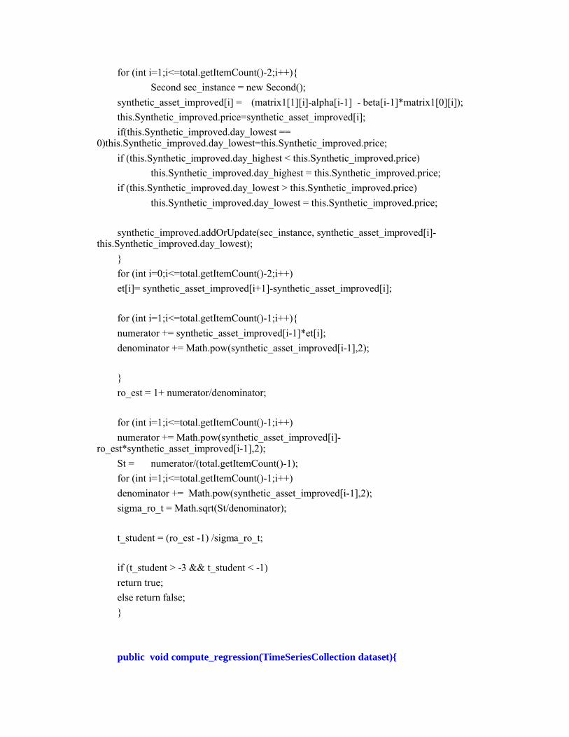
for (int i=1;i<=total.getItemCount()-2;i++){
Second sec_instance = new Second();
synthetic_asset_improved[i] = (matrix1[1][i]-alpha[i-1] - beta[i-1]*matrix1[0][i]);
this.Synthetic_improved.price=synthetic_asset_improved[i];
if(this.Synthetic_improved.day_lowest == 0)this.Synthetic_improved.day_lowest=this.Synthetic_improved.price;
if (this.Synthetic_improved.day_highest < this.Synthetic_improved.price)
this.Synthetic_improved.day_highest = this.Synthetic_improved.price;
if (this.Synthetic_improved.day_lowest > this.Synthetic_improved.price)
this.Synthetic_improved.day_lowest = this.Synthetic_improved.price;
synthetic_improved.addOrUpdate(sec_instance, synthetic_asset_improved[i]-this.Synthetic_improved.day_lowest);
}
for (int i=0;i<=total.getItemCount()-2;i++)
et[i]= synthetic_asset_improved[i+1]-synthetic_asset_improved[i];
for (int i=1;i<=total.getItemCount()-1;i++){
numerator += synthetic_asset_improved[i-1]*et[i];
denominator += Math.pow(synthetic_asset_improved[i-1],2);
}
ro_est = 1+ numerator/denominator;
for (int i=1;i<=total.getItemCount()-1;i++)
numerator += Math.pow(synthetic_asset_improved[i]-ro_est*synthetic_asset_improved[i-1],2);
St = numerator/(total.getItemCount()-1);
for (int i=1;i<=total.getItemCount()-1;i++)
denominator += Math.pow(synthetic_asset_improved[i-1],2);
sigma_ro_t = Math.sqrt(St/denominator);
t_student = (ro_est -1) /sigma_ro_t;
if (t_student > -3 && t_student < -1)
return true;
else return false;
}
public void compute_regression(TimeSeriesCollection dataset){

@SuppressWarnings("unused")
int count;
double mean=0;
for(count = 0;count<total.getItemCount();count++){
mean = mean + matrix1[0][count];}
System.out.println("Mean: \n"+mean/total.getItemCount());
double sigma=0.00001;
for(count = 0;count<total.getItemCount();count++){
sigma += (matrix1[0][count] - mean)*(matrix1[0][count] -mean)/(total.getItemCount()+1);}
sigma = Math.sqrt(sigma);
System.out.println("Sigma: \n"+sigma);
// x1t = A1 . x2t + b [xt]= [A1 1] * x2t
// x1t-1 = A2 . x2t-1 + b [A2 1]
// x1t-2 = A3 . x2t-2 + b [A3 1]
E =new Matrix(Y.minus(X.times(BETA)));
BETA_est = X.transpose().times(X).inverse().times(X.transpose()).times(Y);
E_est = Y.minus(X.times(BETA_est));
System.out.println("Beta1: "+BETA_est.getElement(0, 0)+"Beta2: \n"+BETA_est.getElement(1, 0));
}
/* In Bulding a NN
1)
Start with specifying a linear model and select variables according to AIC Informatio Criterion p171
Using T observations, p exogenous variables including constant.
More variables will lead to a mechanical decrease in the residue error and inverse increase in the log
vraisemblance.
AIC = Akaike Information Criterion = 2*p/T -2*l_est/T where the last term is replaced by
by Ln (Sigma (residu_est square/T))

2)
Use the LM statistic to favor or not a linear (null hypothesis) over non-linear NN model witha single neuron
If the null hypothesis is rejected, test a NN model with one nuron.
3)
test h (null hypothesis) againt h+1 neurons until acceptance of null hypothesis.
*/
// matrix1[0][total.getItemCount()]
void AIC(){
}
Here we compute all first and second derivatives necessary for the Lagrange Multuplier coefficients.
void garch_model()
{
//size_neurons
int h=3;
//h must be superior or equal to the number of regressors
int p=1;
int q=1;
double z=0.5;
double temp = 0;
double [][] temp_ = new double [var_t_r][1];
double [][] temp1 = new double [total.getItemCount()][var_t_r];

double[] yt = new double[total.getItemCount()] ;
double[] et = new double[total.getItemCount()] ;
double[] ht = new double[total.getItemCount()] ;
Matrix dl_dphWe= new Matrix(temp1) ;
Matrix dh_dphWe= new Matrix(temp1) ;
Matrix dl_dteta = new Matrix(new double[total.getItemCount()][4*h]) ;
Matrix df_dteta = new Matrix(new double[total.getItemCount()][4*h]) ;
Matrix dh_dteta = new Matrix(new double[total.getItemCount()][4*h]) ;
Matrix dl_dalpha = new Matrix(new double[total.getItemCount()][p+1+q]) ;
Matrix dh_dalpha = new Matrix(new double[total.getItemCount()][p+1+q]) ;
//initialization of dlt_dphi_dphi
Matrix dlt_dphi_dphWe= new Matrix(new double[total.getItemCount()][p+1+q]) ;
//initialization of dlt_dphi_dteta
Matrix dlt_dphi_dteta = new Matrix(new double[total.getItemCount()][p+1+q]) ;
//initialization of dlt_dphi_dalpha
Matrix dlt_dphi_dalpha = new Matrix(new double[total.getItemCount()][p+1+q]) ;
//initialization of dlt_dteta_dteta
Matrix dlt_dteta_dteta = new Matrix(new double[total.getItemCount()][p+1+q]) ;
//initialization of dlt_dteta_dalpha
Matrix dlt_dteta_dalpha = new Matrix(new double[total.getItemCount()][p+1+q]) ;
//initialization of dlt_dalpha_dalpha
Matrix dlt_dalpha_dalpha = new Matrix(new double[total.getItemCount()][p+1+q]) ;
double[][]xt = new double[total.getItemCount()][var_t_r];
double [] phWe= new double [var_t_r];
double fx_teta = 0;
double [] omega = new double [h]; //number of neurones
double [] gamma = new double [h];
double []w = new double [var_t_r];
double []c = new double [h];
double []lambda = new double [h];
double alpha0 = 0;
double []alpha = new double [p];
double [] beta = new double [q];
double[] F = new double [h];
double [] dF_dgamma = new double [h];
double[] dF_domega = new double [h];;
double[] dF_dc = new double [h];;
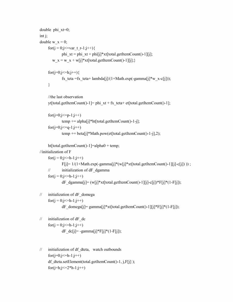
double phi_xt=0;
int j;
double w_x = 0;
for(j = 0;j<=var_t_r-1;j++){
phi_xt = phi_xt + phi[j]*xt[total.getItemCount()-1][j];
w_x = w_x + w[j]*xt[total.getItemCount()-1][j];}
for(j=0;j<=h;j++){
fx_teta =fx_teta+ lambda[j]/(1+Math.exp(-gamma[j]*w_x-c[j]));
}
//the last observation
yt[total.getItemCount()-1]= phi_xt + fx_teta+ et[total.getItemCount()-1];
for(j=0;j<=p-1;j++)
temp += alpha[j]*ht[total.getItemCount()-1-j];
for(j=0;j<=q-1;j++)
temp += beta[j]*Math.pow(et[total.getItemCount()-1-j],2);
ht[total.getItemCount()-1]=alpha0 + temp;
//initialization of F
for(j = 0;j<=h-1;j++)
F[j]= 1/(1+Math.exp(-gamma[j]*(w[j]*xt[total.getItemCount()-1][j]-c[j]) )) ;
// initialization of dF_dgamma
for(j = 0;j<=h-1;j++)
dF_dgamma[j]= (w[j]*xt[total.getItemCount()-1][j]-c[j])*F[j]*(1-F[j]);
// initialization of dF_domega
for(j = 0;j<=h-1;j++)
dF_domega[j]= gamma[j]*xt[total.getItemCount()-1][j]*F[j]*(1-F[j]);
// initialization of dF_dc
for(j = 0;j<=h-1;j++)
dF_dc[j]= -gamma[j]*F[j]*(1-F[j]);
// initialization of df_dteta, watch outbounds
for(j=0;j<=h-1;j++)
df_dteta.setElement(total.getItemCount()-1, j,F[j] );
for(j=h;j<=2*h-1;j++)

df_dteta.setElement(total.getItemCount()-1, j,gamma[j-h]*dF_dgamma[j-h]);
for(j=2*h;j<=3*h-1;j++)
df_dteta.setElement(total.getItemCount()-1, j,gamma[j-2*h]*dF_domega[j-2*h] );
for(j=3*h;j<=4*h-1;j++)
df_dteta.setElement(total.getItemCount()-1, j, gamma[j-3*h]*dF_dc[j-3*h]);
//initialization of dh_dalpha, watch outbounds
dh_dalpha.setElement(total.getItemCount()-1, 0,1 );
for(j=1;j<=p;j++)
dh_dalpha.setElement(total.getItemCount()-1, j,ht[total.getItemCount()-2-j] );
for(j=p+1;j<=p+q;j++)
dh_dalpha.setElement(total.getItemCount()-1, j,Math.pow(et[total.getItemCount()-2-j],2) );
// initialization of dh_dphi, watch outbounds
for(j=0;j<= var_t_r-1;j++)
for(int k=0;k<=p-1;k++)
dh_dphi.setElement(total.getItemCount()-1, j,alpha[k]*dh_dphi.getElement(total.getItemCount()-2-k, j) );
for(j=0;j<= var_t_r-1;j++)
for(int k=p;k<=p+q;k++)
dh_dphi.setElement(total.getItemCount()-1, j,dh_dphi.getElement(total.getItemCount()-1, j)-2*beta[k]*et[total.getItemCount()-2-k]*xt[total.getItemCount()-2-k][j]);
//initialization of dh_dteta
for(j=0;j<= 4*h-1;j++)
for(int k=0;k<=p-1;k++)
dh_dteta.setElement(total.getItemCount()-1, j,alpha[k]*dh_dteta.getElement(total.getItemCount()-2-k, j) );
for(j=0;j<= 4*h-1;j++)
for(int k=p;k<=p+q;k++)
dh_dteta.setElement(total.getItemCount()-1, j,dh_dteta.getElement(total.getItemCount()-1, j)-2*beta[k]*et[total.getItemCount()-2-k]*df_dteta.getElement(total.getItemCount()-2-k, j));

for(j=0;j<= var_t_r-1;j++)
dl_dphi.setElement(total.getItemCount()-1,j, et[total.getItemCount()-1]/ht[total.getItemCount()-1] *xt[total.getItemCount()-1][j] + .5*dh_dphi.getElement(total.getItemCount()-1, j)/ht[total.getItemCount()-1]*(Math.pow(et[total.getItemCount()-1],2)/ht[total.getItemCount()-1]-1));
for(j=0;j<= 4*h-1;j++)
dl_dteta.setElement(total.getItemCount()-1, j, et[total.getItemCount()-1]/ht[total.getItemCount()-1]*df_dteta.getElement(total.getItemCount()-1,j)+.5*dh_dteta.getElement(total.getItemCount()-1, j)/ht[total.getItemCount()-1]*(Math.pow(et[total.getItemCount()-1],2)/ht[total.getItemCount()-1]-1));
for(j=0;j<=p+q;j++)
dl_dalpha.setElement(total.getItemCount()-1, j, .5/ht[total.getItemCount()-1]*(Math.pow(et[total.getItemCount()-1],2)/ht[total.getItemCount()-1]-1)*dh_dalpha.getElement(total.getItemCount()-1, j));
//initialization of hessian of log likelyhood Ht
//initialization of dlt_dphi_dphi
// initialization of dlt_dphi_dteta
// initialization of dlt_dphi_dalpha
// initialization of dlt_dteta_dteta
// initialization of dlt_dteta_dalpha
// initialization of dlt_dalpha_dalpha
}
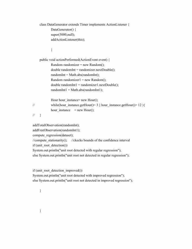
class DataGenerator extends Timer implements ActionListener {
DataGenerator() {
super(5000,null);
addActionListener(this);
}
public void actionPerformed(ActionEvent event) {
Random randomizer = new Random();
double randomInt = randomizer.nextDouble();
randomInt = Math.abs(randomInt);
Random randomizer1 = new Random();
double randomInt1 = randomizer1.nextDouble();
randomInt1 = Math.abs(randomInt1);
Hour hour_instance= new Hour();
// while(hour_instance.getHour()< 3 || hour_instance.getHour()> 12 ){
hour_instance = new Hour();
// }
addTotalObservation(randomInt);
addFreeObservation(randomInt1);
compute_regression(dataset);
//compute_stationarity(); //ckecks bounds of the confidence interval
if (unit_root_detection())
System.out.println("unit root detected with regular regression");
else System.out.println("unit root not detected in regular regression");
if (unit_root_detection_improved())
System.out.println("unit root detected with improved regression");
else System.out.println("unit root not detected in improved regression");
}
}

public static void main(String[] args) {
JFrame frame = new JFrame("Share Price Time Series");
TimeSeriesMain panel = new TimeSeriesMain();
frame.getContentPane().add(panel, BorderLayout.CENTER);
frame.setBounds(200, 120, 600, 280);
frame.setVisible(true);
panel.new DataGenerator().start();
frame.addWindowListener(new WindowAdapter() {
@Override
public void windowClosing(WindowEvent e) {
System.exit(0);
}
});
}
}
The extractor of stocks from the website: www.boursorama.com
my $link1 = "http://www.boursorama.com/cours.phtml?symbole=1rPAC"; # Accor
my $link2 = "http://www.boursorama.com/cours.phtml?symbole=1rPADE"; # Adecco
$pid = fork();
if($pid==0){
exec "perl arbitrage_trading.pl Accor $link1";}
else {
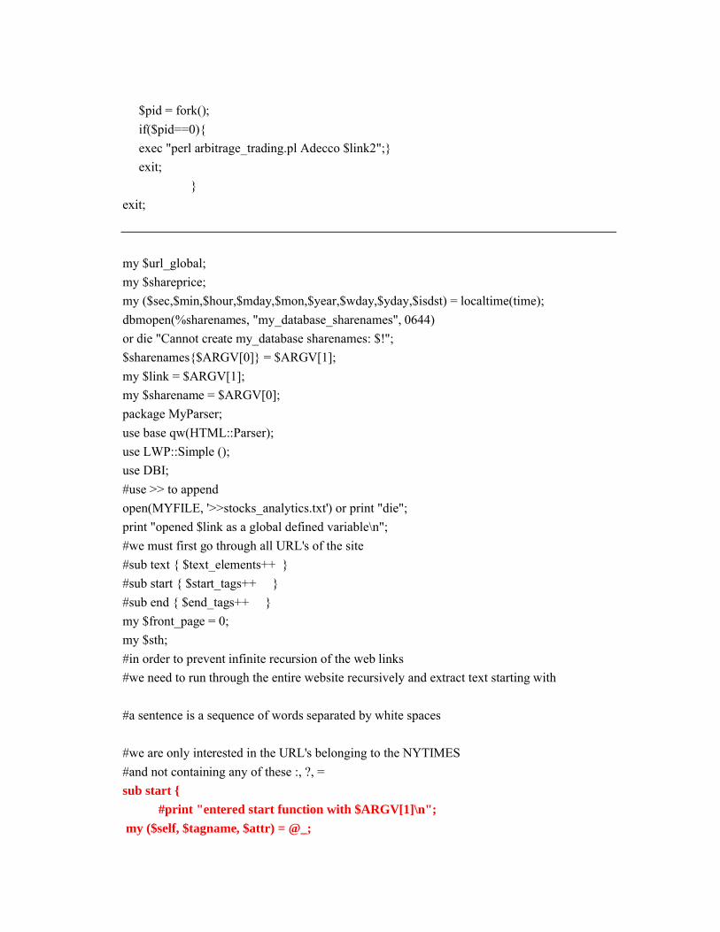
$pid = fork();
if($pid==0){
exec "perl arbitrage_trading.pl Adecco $link2";}
exit;
}
exit;
my $url_global;
my $shareprice;
my ($sec,$min,$hour,$mday,$mon,$year,$wday,$yday,$isdst) = localtime(time);
dbmopen(%sharenames, "my_database_sharenames", 0644)
or die "Cannot create my_database sharenames: $!";
$sharenames{$ARGV[0]} = $ARGV[1];
my $link = $ARGV[1];
my $sharename = $ARGV[0];
package MyParser;
use base qw(HTML::Parser);
use LWP::Simple ();
use DBI;
#use >> to append
open(MYFILE, '>>stocks_analytics.txt') or print "die";
print "opened $link as a global defined variable\n";
#we must first go through all URL's of the site
#sub text { $text_elements++ }
#sub start { $start_tags++ }
#sub end { $end_tags++ }
my $front_page = 0;
my $sth;
#in order to prevent infinite recursion of the web links
#we need to run through the entire website recursively and extract text starting with
#a sentence is a sequence of words separated by white spaces
#we are only interested in the URL's belonging to the NYTIMES
#and not containing any of these :, ?, =
sub start {
#print "entered start function with $ARGV[1]\n";
my ($self, $tagname, $attr) = @_;

#GET SHARE NAME WITH A HASH
}
#>107.91(c) EUR
sub text {
my ($self,$text) = @_;
$_ = $text;
my ($sec2,$min2,$hour2,$mday2,$mon2,$year2,$wday2,$yday2,$isdst2) = localtime(time);
if (/\d*\.\d*\(c\) EUR/ ) {
# if($hour2>= 3 && $hour2<= 12) {
print MYFILE "$sharename $_ ";
print MYFILE scalar localtime();
print MYFILE "\n\n";
print "$sharename $_ ";
print scalar localtime();
print "\n\n";
# else { print "not yet time scalar localtime()\n"; }
close (MYFILE);
open(MYFILE, '>>stocks_analytics.txt') or print "die";
}
else {
#print "$text\n";
}
}
#class="p2b">9.85(c) EUR</TD>
package main;
#sub arbitrage {
#print "$sharename $link";

#print scalar localtime();
#print "\n";
#use AWEto adjust the price of share to the index weighted average:
#Discern and Predict own share trend using current daily data and past weighted daily data
#[size of further move down if trend is down and for current share price level]
#[ ]
#[ ]
#Discern and Predict similar share categories:
#Discern and Predict Market trend:
#}
# Test the parser
my $sec1 = $sec;
my $min1 = $min;
my $parser1 = MyParser->new;
my ($sec1,$min1,$hour1,$mday1,$mon1,$year1,$wday1,$yday1,$isdst1) = localtime(time);
while(1) {
my ($sec1,$min1,$hour1,$mday1,$mon1,$year1,$wday1,$yday1,$isdst1) = localtime(time);
if ( ($sec1-$sec) ==10 && ( $sec1 > $sec) ){
#print "OK\n";
my $parser1 = MyParser->new;
$parser1->parse( LWP::Simple::get($link) );
$sec= $sec1;
#arbitrage();
}
if($sec1 < $sec) { $sec = -(60-$sec);}
}
close (MYFILE);

References:(1) Financial statistical modelling with a new nature-inspired Technique, Nikos S. Thomaidis_1, George D. Dounias1, and Nick Kondakis1,2