attachment d-7: rebound and uplift of the stilling basin ... · figure 40 flac model in dis...

Attachment D-7: Rebound and Uplift of the Stilling Basin, Deep Soil Mixing Design

Attachment D-7:

Rebound and Uplift of the Stilling Basin, Deep Soil Mixing Design

Fargo Moorhead Metropolitan Area Draft Design Documentation Report Flood Risk Management Project Inlet Diversion Appendix D, Attachment 7: FLAC Analysis of DIS Rebound

DDR_FMM_DIS_App_D_Attach_7_FLAC_Analysis_draft.docx

Appendix D, Attachment 7: FLAC Analysis of Diversion

Inlet Structure Rebound

Fargo Moorhead Metropolitan Area

Flood Risk Management Project

Diversion Inlet Structure

Engineering and Design Phase

Doc Version: Draft

February 22, 2016


DDR_FMM_DIS_App_D_Attach_7_FLAC_Analysis_draft.docx

This page is intentionally left blank


DDR_FMM_DIS_App_D_Attach_7_FLAC_Analysis_draft.docx Appendix D, Attachment 7: Page i

Appendix D, Attachment 7: FLAC Analysis of Diversion Inlet Structure Rebound

Table of Contents 1. General .................................................................................................................................................. 1

2. Stratigraphy ........................................................................................................................................... 1

3. Soil Expansion ....................................................................................................................................... 2

4. Soil Parameters ..................................................................................................................................... 2

4.1. General .......................................................................................................................................... 2

4.2. Modified Cam Clay Parameters .................................................................................................... 3

4.3. Shear Strength Parameters ........................................................................................................... 4

5. Free Field Unloading ............................................................................................................................. 4

5.1. FLAC Modeling Procedure ............................................................................................................. 4

5.2. FLAC Modeling Results .................................................................................................................. 6

6. Unloading with Pile and Structure Present ........................................................................................... 6

6.1. FLAC Modeling Procedure ............................................................................................................. 6

6.2. Pile Elements ................................................................................................................................. 8

6.3. Pile-Soil Shear Coupling Springs .................................................................................................... 8

6.4. FLAC Modeling Results .................................................................................................................. 9

6.4.1 Stilling Basin Location ........................................................................................................... 9

6.4.2 Shear Transfer in the Till ..................................................................................................... 10

6.4.3 Approach Apron .................................................................................................................. 10

6.4.4 Control Structure ................................................................................................................ 11

7. Mitigation of Stilling Basin Rebound ................................................................................................... 12

7.1. FLAC Modeling Results ................................................................................................................ 12

7.2. Deep Soil Mixing Plan .................................................................................................................. 14

8. Conclusions ......................................................................................................................................... 14

9. References .......................................................................................................................................... 15

10. District Quality Control ....................................................................................................................... 15


DDR_FMM_DIS_App_D_Attach_7_FLAC_Analysis_draft.docx Appendix D, Attachment 7: Page ii

TABLES Table 1 Summary of Mohr-Coulomb Parameters ......................................................................................... 3

Table 2 Summary of Modified Cam-Clay Parameters .................................... Error! Bookmark not defined.

Table 3 Structural Parameters ....................................................................... Error! Bookmark not defined.

Table 4 Comparison of Axial Load and Displacement for Varying 𝛽𝛽 Values in the Till (Stilling Basin Location) ..................................................................................................................................................... 10

Table 5 Comparison of Axial Load and Displacement for Varying 𝛽𝛽 Values in the Till (Stilling Basin and Approach Apron Locations) ........................................................................................................................ 11

Table 6 Mohr-Coulomb Parameters for Improved Soil............................................................................... 13

FIGURES Figure 1 Plan View of Diversion Inlet .......................................................................................................... 16

Figure 2 Profile of Diversion Channel, Structure, and Connecting Channel ............................................... 17

Figure 3 Boring Log 15-233M ...................................................................................................................... 18

Figure 4 Boring Log 14-210M ...................................................................................................................... 19

Figure 5 Determination of Reference Specific Volume and Preconsolidation Pressure for the Argusville Fm. .............................................................................................................................................................. 20

Figure 6 Determination of Reference Specific Volume and Preconsolidation Pressure for the Brenna Fm. .................................................................................................................................................................... 21

Figure 7 Stratigraphy for FLAC modeling at the Diversion Inlet ................................................................. 22

Figure 8 Effective Vertical Stress Contours for Insitu Conditions ............................................................... 23

Figure 9 Effective Horizontal Stress Contours for Insitu Conditions ........................................................... 24

Figure 10 Comparison of Hand Calculated Vertical and Horizontal Effective Stress Profiles to FLAC ........ 25

Figure 11 Effective Vertical Stress Contours after Unloading to Elevation 888 ft. ..................................... 26

Figure 12 Effective Horizontal Stress Contours after Unloading to Elevation 888 ft. ................................. 27

Figure 13 Vertical Displacement Contours after Unloading to Elevation 888 ft......................................... 28

Figure 14 Rebound Profile Comparison of FLAC to One Dimensional Expansion Spreadsheet Calculation .................................................................................................................................................................... 29

Figure 15 Location of the Single Pile FLAC Model in the DIS Stilling Basin ................................................. 30

Figure 16 FLAC model in DIS Stilling Basin with Pile and Pile Cap (prior to unloading) .............................. 31


DDR_FMM_DIS_App_D_Attach_7_FLAC_Analysis_draft.docx Appendix D, Attachment 7: Page iii

Figure 17 Effective Vertical Stress Contours, 250 psf Contour Interval, DIS Stilling Basin ......................... 32

Figure 18 Effective Horizontal Stress Contours, 250 psf Contour Interval, DIS Stilling Basin ..................... 33

Figure 19 Effective Vertical Stress Contours, 50 psf Contour Interval, DIS Stilling Basin ........................... 34

Figure 20 Shear Strain Rate Contours, DIS Stilling Basin ............................................................................ 35

Figure 21 Vertical Displacement Contours, DIS Stilling Basin ..................................................................... 36

Figure 22 Axial Load in Pile, DIS Stilling Basin ............................................................................................. 37

Figure 23 Shear Spring Forces, DIS Stilling Basin ........................................................................................ 38

Figure 24 Pile Displacement, DIS Stilling Basin ........................................................................................... 39

Figure 25 Location of the Single Pile FLAC Model in the DIS Approach Apron .......................................... 40

Figure 26 FLAC model in DIS Approach Apron with Pile and Pile Cap (after unloading) ............................ 41

Figure 27 Effective Vertical Stress Contours, 250 psf Contour Interval, DIS Approach Apron ................... 42

Figure 28 Effective Horizontal Stress Contours, 250 psf Contour Interval, DIS Approach Apron ............... 43

Figure 29 Effective Vertical Stress Contours, 50 psf Contour Interval, DIS Approach Apron ..................... 44

Figure 30 Shear Strain Rate Contours, DIS Approach Apron ...................................................................... 45

Figure 31 Vertical Displacement Contours, DIS Approach Apron ............................................................... 46

Figure 32 Axial Load in Pile, DIS Approach Apron ....................................................................................... 47

Figure 33 Shear Spring Force, DIS Approach Apron .................................................................................... 48

Figure 34 Pile Displacement, DIS Approach Apron ..................................................................................... 49

Figure 35 Location of the Control Structure FLAC Model Cross-Section .................................................... 50

Figure 36 FLAC Model of DIS Control Structure (after unloading) .............................................................. 51

Figure 37 Effective Vertical Stress Contours, DIS Control Structure (after unloading)............................... 52

Figure 38 Effective Horizontal Stress Contours, DIS Control Structure ...................................................... 53

Figure 39 Vertical Displacement Contours, DIS Control Structure ............................................................. 54

Figure 40 FLAC Model in DIS Stilling Basin with Pile, Pile Cap and DSM Treated Zones (after unloading) 55

Figure 41 Effective Vertical Stress Contours, 500 psf Contour Interval, DIS Stilling Basin with DSM Treated Zones ........................................................................................................................................................... 56

Figure 42 Effective Horizontal Stress Contours, 500 psf Contour Interval, DIS Stilling Basin with DSM Treated Zones ............................................................................................................................................. 57

Figure 43 Effective Vertical Stress Contours, 50 psf Contour Interval, DIS Stilling Basin with DSM Treated Zones ........................................................................................................................................................... 58

Figure 44 Shear Strain Rate Contours, DIS Stilling Basin with DSM Treated Zones .................................... 59


DDR_FMM_DIS_App_D_Attach_7_FLAC_Analysis_draft.docx Appendix D, Attachment 7: Page iv

Figure 45 Shear Stress Contours, 25 psf Contour Interval, DIS Stilling Basin with DSM Treated Zones ..... 60

Figure 46 Shear Stress Contours, 50 psf Contour Interval, DIS Stilling Basin with DSM Treated Zones ..... 61

Figure 47 Vertical Displacement Contours, DIS Stilling Basin with DSM Treated Zones ............................ 62

Figure 48 Axial Load in Pile, DIS Stilling Basin with DSM Treated Zones .................................................... 63

Figure 49 Pile Displacement, DIS Stilling Basin with DSM Treated Zones .................................................. 64

Figure 50 Proposed DSM Panel Layout for DIS Stilling Basin ...................................................................... 65


DDR_FMM_DIS_App_D_Attach_7_FLAC_Analysis_draft.docx Appendix D, Attachment 7

Executive Summary

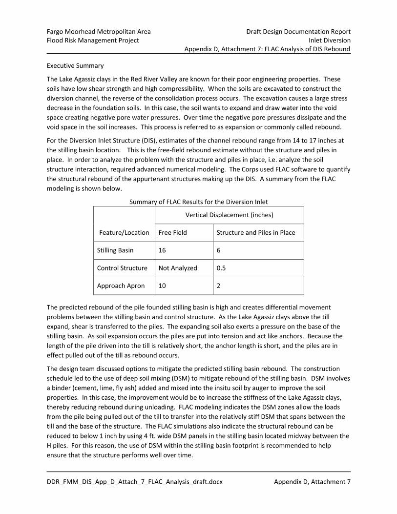
The Lake Agassiz clays in the Red River Valley are known for their poor engineering properties. These soils have low shear strength and high compressibility. When the soils are excavated to construct the diversion channel, the reverse of the consolidation process occurs. The excavation causes a large stress decrease in the foundation soils. In this case, the soil wants to expand and draw water into the void space creating negative pore water pressures. Over time the negative pore pressures dissipate and the void space in the soil increases. This process is referred to as expansion or commonly called rebound.

For the Diversion Inlet Structure (DIS), estimates of the channel rebound range from 14 to 17 inches at the stilling basin location. This is the free-field rebound estimate without the structure and piles in place. In order to analyze the problem with the structure and piles in place, i.e. analyze the soil structure interaction, required advanced numerical modeling. The Corps used FLAC software to quantify the structural rebound of the appurtenant structures making up the DIS. A summary from the FLAC modeling is shown below.

Summary of FLAC Results for the Diversion Inlet

Feature/Location

Vertical Displacement (inches)

Free Field Structure and Piles in Place

Stilling Basin 16 6

Control Structure Not Analyzed 0.5

Approach Apron 10 2

The predicted rebound of the pile founded stilling basin is high and creates differential movement problems between the stilling basin and control structure. As the Lake Agassiz clays above the till expand, shear is transferred to the piles. The expanding soil also exerts a pressure on the base of the stilling basin. As soil expansion occurs the piles are put into tension and act like anchors. Because the length of the pile driven into the till is relatively short, the anchor length is short, and the piles are in effect pulled out of the till as rebound occurs.

The design team discussed options to mitigate the predicted stilling basin rebound. The construction schedule led to the use of deep soil mixing (DSM) to mitigate rebound of the stilling basin. DSM involves a binder (cement, lime, fly ash) added and mixed into the insitu soil by auger to improve the soil properties. In this case, the improvement would be to increase the stiffness of the Lake Agassiz clays, thereby reducing rebound during unloading. FLAC modeling indicates the DSM zones allow the loads from the pile being pulled out of the till to transfer into the relatively stiff DSM that spans between the till and the base of the structure. The FLAC simulations also indicate the structural rebound can be reduced to below 1 inch by using 4 ft. wide DSM panels in the stilling basin located midway between the H piles. For this reason, the use of DSM within the stilling basin footprint is recommended to help ensure that the structure performs well over time.


DDR_FMM_DIS_App_D_Attach_7_FLAC_Analysis_draft.docx Appendix D, Attachment 7: Page 1

Appendix D, Attachment 7: FLAC Analysis of Diversion Inlet Structure Rebound

1. General The Diversion Inlet Structure (DIS) is a pile-founded hydraulic structure that consists of the following major components: approach apron, control structure, and stilling basin. The approach apron and stilling basin are founded on vertical HP14x73 piles generally spaced between 8 and 10 ft. on center. The control structure includes the tainter gates, stepped spillway, mechanical platform, and vehicle service bridge. The control structure is founded on HP14x73 piles battered in both the upstream and downstream directions with vertical piles located under the piers. The DIS provides water control and grade change from the connecting channel into the diversion channel. Figure 1 and Figure 2 provide a plan and profile view of the Diversion Inlet Structure, the connecting channel, and the diversion channel.

The purpose of this report is to estimate the structural rebound of the primary components of the DIS to allow the component structural joints to be properly designed and detailed for any anticipated differential movement. In order to accomplish this, the finite difference program Fast Lagrangian Analysis of Continua (FLAC) 7.0 by Itasca Consulting Group, Inc. was used to conduct numerical analyses of the soil structure interaction. In general, the report explains the methodology used in the various FLAC models, describes the conditions analyzed, discusses the model results and validations, and illustrates soil-structure response through a series of figures.

2. Stratigraphy

The stratigraphy for the FLAC model is similar to what was used in the limit equilibrium slope stability analyses for determining unbalanced loads and documented in Appendix D: Geotechnical Engineering and Geology. The soil stratigraphy was based primarily on two borings located along the diversion centerline. Soil boring 14-210M (Figure 4) is located at the downstream end of the DIS stilling basin and boring 15-232M (Figure 3) is located near the center of the control structure. The details of the stratigraphy are as follows:

• Ground surface in the area averages El. 915 ft. and it was assumed the natural ground water table was approximately 10 feet below ground surface at El. 905 ft.

• The Sherack/Brenna contact ranges from El. 898 ft. to 889 ft. An elevation of 890 ft. was used which was the average between borings 14-210M and 15-232M.

• The Brenna/Argusville contact ranges from El. 869 ft. to 860 ft. An elevation of 863 ft. was used which is about the average contact elevation between borings 14-210M and 15-232M.

• The Argusville/Unit “A” Till contact ranges from El. 852 ft. to 845 ft. An elevation of 848 ft. was used which is the contact elevation from boring 14-210M.

• The Weathered Till/Intact Till contact was chosen as El. 840 ft, or 8 feet into the till.



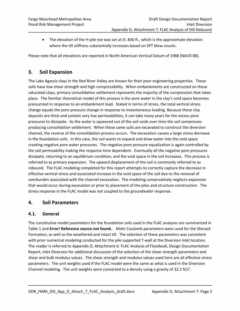
• The elevation of the H-pile toe was set at El. 836 ft., which is the approximate elevation where the till stiffness substantially increases based on SPT blow counts.

Please note that all elevations are reported in North American Vertical Datum of 1988 (NAVD 88).

3. Soil Expansion The Lake Agassiz clays in the Red River Valley are known for their poor engineering properties. These soils have low shear strength and high compressibility. When embankments are constructed on these saturated clays, primary consolidation settlement represents the majority of the compression that takes place. The familiar theoretical model of this process is the pore water in the clay’s void space becomes pressurized in response to an embankment load. Stated in terms of stress, the total vertical stress change equals the pore pressure change in response to instantaneous loading. Because these clay deposits are thick and contain very low permeabilities, it can take many years for the excess pore pressures to dissipate. As the water is squeezed out of the soil voids over time the soil compresses producing consolidation settlement. When these same soils are excavated to construct the diversion channel, the reverse of the consolidation process occurs. The excavation causes a large stress decrease in the foundation soils. In this case, the soil wants to expand and draw water into the void space creating negative pore water pressures. The negative pore pressure equalization is again controlled by the soil permeability making the response time dependent. Eventually all the negative pore pressures dissipate, returning to an equilibrium condition, and the void space in the soil increases. This process is referred to as primary expansion. The upward displacement of the soil is commonly referred to as rebound. The FLAC modeling completed for this report attempts to correctly capture the decrease in effective vertical stress and associated increase in the void space of the soil due to the removal of overburden associated with the channel excavation. The modeling conservatively neglects expansion that would occur during excavation or prior to placement of the piles and structure construction. The stress response in the FLAC model was not coupled to the groundwater response.

4. Soil Parameters

4.1. General

The constitutive model parameters for the foundation soils used in the FLAC analyses are summarized in Table 1 and Error! Reference source not found.. Mohr Coulomb parameters were used for the Sherack Formation, as well as the weathered and intact till. The selection of these parameters was consistent with prior numerical modeling conducted for the pile supported T-wall at the Diversion Inlet location. The reader is referred to Appendix D, Attachment 6: FLAC Analysis of Floodwall, Design Documentation Report, Inlet Diversion for additional discussion of the selection of the shear strength parameters and shear and bulk modulus values. The shear strength and modulus values used here are all effective stress parameters. The unit weights used if the FLAC model were the same as what is used in the Diversion Channel modeling. The unit weights were converted to a density using a gravity of 32.2 ft/s2.



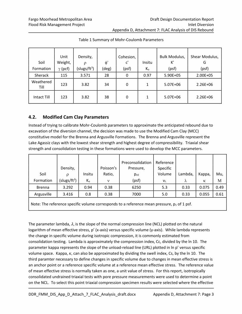
Table 1 Summary of Mohr-Coulomb Parameters

Unit Density, Cohesion, Bulk Modulus, Shear Modulus,

Soil Weight, ρ φ' c' Insitu K' G Formation γ (pcf) (slugs/ft3) (deg) (psf) Ko (psf) (psf)

Sherack 115 3.571 28 0 0.97 5.90E+05 2.00E+05 Weathered

Till 123 3.82 34 0 1 5.07E+06 2.26E+06

Intact Till 123 3.82 38 0 1 5.07E+06 2.26E+06

4.2. Modified Cam Clay Parameters Instead of trying to calibrate Mohr-Coulomb parameters to approximate the anticipated rebound due to excavation of the diversion channel, the decision was made to use the Modified Cam Clay (MCC) constitutive model for the Brenna and Argusville Formations. The Brenna and Argusville represent the Lake Agassiz clays with the lowest shear strength and highest degree of compressibility. Triaxial shear strength and consolidation testing in these formations were used to develop the MCC parameters.

Preconsolidation Reference

Density, Poisson's Pressure, Specific Soil ρ Insitu Ratio, pc0 Volume Lambda, Kappa, Mu,

Formation (slugs/ft3) Ko ν (psf) vλ λ κ Μ Brenna 3.292 0.94 0.38 6250 5.3 0.33 0.075 0.49

Argusville 3.416 0.8 0.38 7000 5.0 0.33 0.055 0.61

Note: The reference specific volume corresponds to a reference mean pressure, p1 of 1 psf.

The parameter lambda, 𝜆𝜆, is the slope of the normal compression line (NCL) plotted on the natural logarithm of mean effective stress, p’ (x-axis) versus specific volume (y-axis). While lambda represents the change in specific volume during isotropic compression, it is commonly estimated from consolidation testing. Lambda is approximately the compression index, Cc, divided by the ln 10. The parameter kappa represents the slope of the unload-reload line (URL) plotted in ln p’ versus specific volume space. Kappa, 𝜅𝜅, can also be approximated by dividing the swell index, Cs, by the ln 10. The third paramter necessary to define changes in specific volume due to changes in mean effective stress is an anchor point or a reference specific volume at a reference mean effective stress. The reference value of mean effective stress is normally taken as one, a unit value of stress. For this report, isotropically consolidated undrained triaxial tests with pore pressure measurements were used to determine a point on the NCL. To select this point triaxial compression specimen results were selected where the effective



confining stress was judged to be above the preconsolidation stress meaning the effective confining stress represented the mean effective stress and the void ratio after consolidation determined the specific volume for a point on the NCL. Projecting these values back to a p’ value of 1 psf at a slope of lambda gives an estimate of the reference specific volume. Figure 5 and Figure 6 show the determination of the reference specific volume from triaxial testing for the Argusville and Brenna formations respectively.

The lambda and kappa values that were used in the FLAC modeling were increased 10 to 20% above the swell index values from consolidation testing to achieve a better calibration to the one dimensional hand calculation. The rebound computations in FLAC were found to be sensitive to the selection of Kappa and the reference specific volume. Slightly decreasing the reference specific volume increased the rebound in FLAC. Changes to Kappa were directly proportional to the rebound determined in FLAC.

The parameter, Μ, is slope of the critical state line (CSL). For triaxial compression testing, Μ, is determined from: Μ = (6𝑠𝑠𝑠𝑠𝑠𝑠𝑠𝑠′)/(3− 𝑠𝑠𝑠𝑠𝑠𝑠𝑠𝑠′). The preconsolidation pressure used in the MCC model can be determined by estimating the preconsolidation pressure from consolidation testing and assuming this is the maximum effective vertical stress. The maximum effective horizontal stress can then be determined from an estimate of the at rest earth pressure coefficient. From these values the maximum mean effective stress and maximum deviatoric stress can be estimated. The preconsolidation stress 𝑝𝑝𝑐𝑐0 used in the MCC model can be calculated as:

𝑞𝑞2 = 𝑀𝑀2[𝑝𝑝(𝑝𝑝𝑐𝑐0 − 𝑝𝑝)] where p=maximum mean effective stress and q is the maximum deviatoric stress

The determination of the preconsolidation stress is illustrated in the Theory and Background FLAC manual under Modified Cam-Clay constitutive model. Rebound computations in FLAC were found to be insensitive to the selection of the preconsolidation pressure. The calculation of the preconsolidation pressure, 𝑝𝑝𝑐𝑐0 is shown in Figure 5 and Figure 6.

4.3. Shear Strength Parameters

The effective and total stress shear strength parameters are not directly discussed in this report. The reader is referred to Sections 3.2 and 3.3 of Appendix D, Attachment 6: FLAC Analysis of Floodwall of the Design Documentation Report of the Inlet Diversion.

5. Free Field Unloading

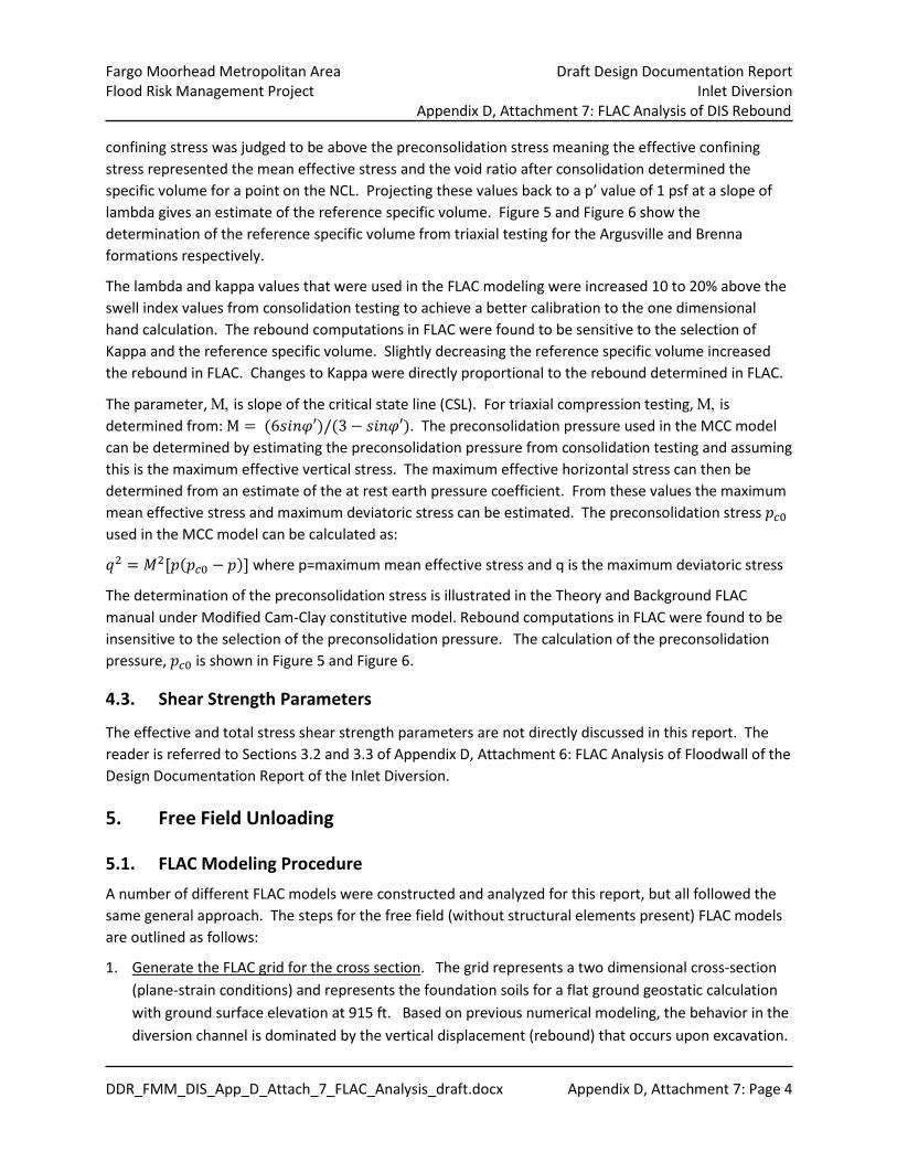
5.1. FLAC Modeling Procedure A number of different FLAC models were constructed and analyzed for this report, but all followed the same general approach. The steps for the free field (without structural elements present) FLAC models are outlined as follows:

1. Generate the FLAC grid for the cross section. The grid represents a two dimensional cross-section (plane-strain conditions) and represents the foundation soils for a flat ground geostatic calculation with ground surface elevation at 915 ft. Based on previous numerical modeling, the behavior in the diversion channel is dominated by the vertical displacement (rebound) that occurs upon excavation.



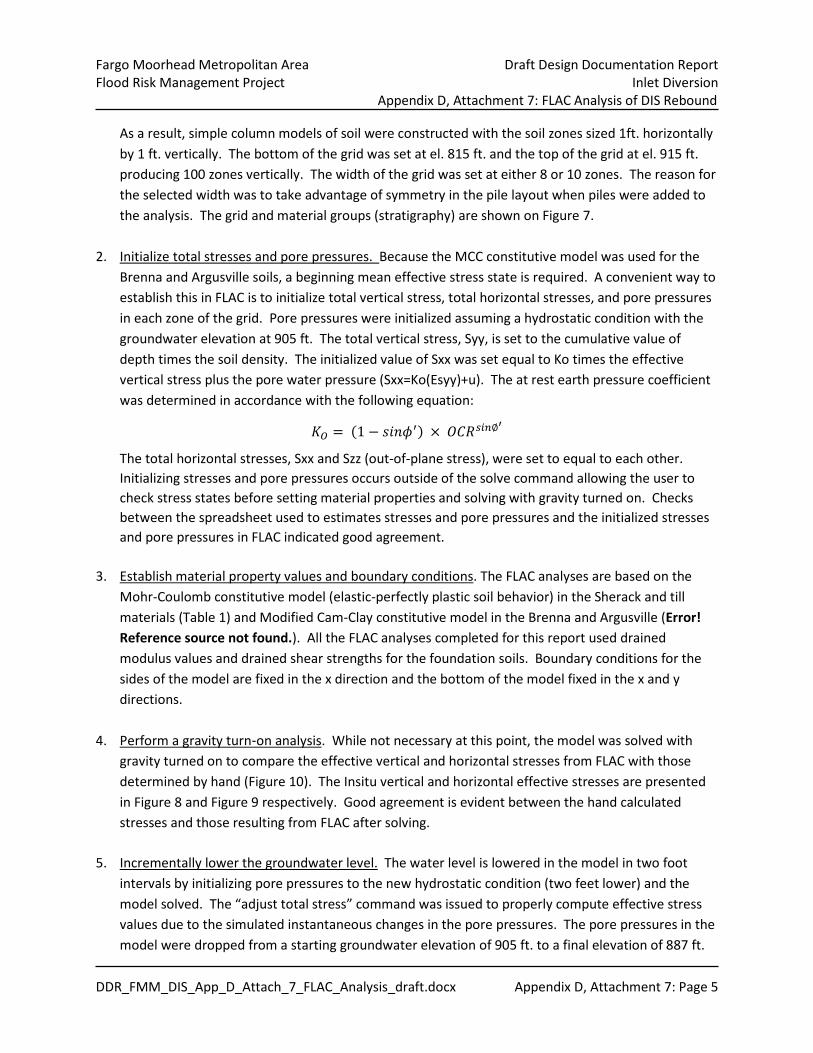
As a result, simple column models of soil were constructed with the soil zones sized 1ft. horizontally by 1 ft. vertically. The bottom of the grid was set at el. 815 ft. and the top of the grid at el. 915 ft. producing 100 zones vertically. The width of the grid was set at either 8 or 10 zones. The reason for the selected width was to take advantage of symmetry in the pile layout when piles were added to the analysis. The grid and material groups (stratigraphy) are shown on Figure 7.

2. Initialize total stresses and pore pressures. Because the MCC constitutive model was used for the Brenna and Argusville soils, a beginning mean effective stress state is required. A convenient way to establish this in FLAC is to initialize total vertical stress, total horizontal stresses, and pore pressures in each zone of the grid. Pore pressures were initialized assuming a hydrostatic condition with the groundwater elevation at 905 ft. The total vertical stress, Syy, is set to the cumulative value of depth times the soil density. The initialized value of Sxx was set equal to Ko times the effective vertical stress plus the pore water pressure (Sxx=Ko(Esyy)+u). The at rest earth pressure coefficient was determined in accordance with the following equation:

𝐾𝐾𝑂𝑂 = (1 − 𝑠𝑠𝑠𝑠𝑠𝑠𝜙𝜙′) × 𝑂𝑂𝑂𝑂𝑂𝑂𝑠𝑠𝑠𝑠𝑠𝑠∅′

The total horizontal stresses, Sxx and Szz (out-of-plane stress), were set to equal to each other. Initializing stresses and pore pressures occurs outside of the solve command allowing the user to check stress states before setting material properties and solving with gravity turned on. Checks between the spreadsheet used to estimates stresses and pore pressures and the initialized stresses and pore pressures in FLAC indicated good agreement.

3. Establish material property values and boundary conditions. The FLAC analyses are based on the Mohr-Coulomb constitutive model (elastic-perfectly plastic soil behavior) in the Sherack and till materials (Table 1) and Modified Cam-Clay constitutive model in the Brenna and Argusville (Error! Reference source not found.). All the FLAC analyses completed for this report used drained modulus values and drained shear strengths for the foundation soils. Boundary conditions for the sides of the model are fixed in the x direction and the bottom of the model fixed in the x and y directions.

4. Perform a gravity turn‐on analysis. While not necessary at this point, the model was solved with gravity turned on to compare the effective vertical and horizontal stresses from FLAC with those determined by hand (Figure 10). The Insitu vertical and horizontal effective stresses are presented in Figure 8 and Figure 9 respectively. Good agreement is evident between the hand calculated stresses and those resulting from FLAC after solving.

5. Incrementally lower the groundwater level. The water level is lowered in the model in two foot

intervals by initializing pore pressures to the new hydrostatic condition (two feet lower) and the model solved. The “adjust total stress” command was issued to properly compute effective stress values due to the simulated instantaneous changes in the pore pressures. The pore pressures in the model were dropped from a starting groundwater elevation of 905 ft. to a final elevation of 887 ft.



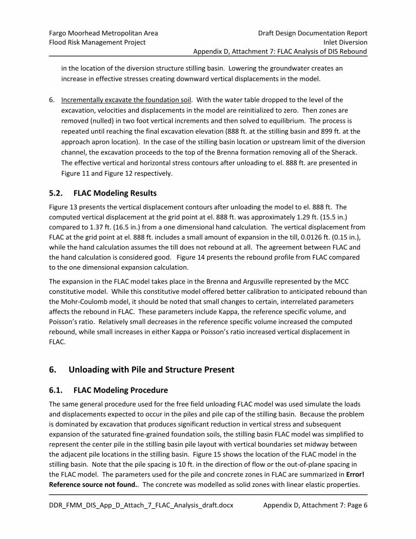
in the location of the diversion structure stilling basin. Lowering the groundwater creates an increase in effective stresses creating downward vertical displacements in the model.

6. Incrementally excavate the foundation soil. With the water table dropped to the level of the

excavation, velocities and displacements in the model are reinitialized to zero. Then zones are removed (nulled) in two foot vertical increments and then solved to equilibrium. The process is repeated until reaching the final excavation elevation (888 ft. at the stilling basin and 899 ft. at the approach apron location). In the case of the stilling basin location or upstream limit of the diversion channel, the excavation proceeds to the top of the Brenna formation removing all of the Sherack. The effective vertical and horizontal stress contours after unloading to el. 888 ft. are presented in Figure 11 and Figure 12 respectively.

5.2. FLAC Modeling Results Figure 13 presents the vertical displacement contours after unloading the model to el. 888 ft. The computed vertical displacement at the grid point at el. 888 ft. was approximately 1.29 ft. (15.5 in.) compared to 1.37 ft. (16.5 in.) from a one dimensional hand calculation. The vertical displacement from FLAC at the grid point at el. 888 ft. includes a small amount of expansion in the till, 0.0126 ft. (0.15 in.), while the hand calculation assumes the till does not rebound at all. The agreement between FLAC and the hand calculation is considered good. Figure 14 presents the rebound profile from FLAC compared to the one dimensional expansion calculation.

The expansion in the FLAC model takes place in the Brenna and Argusville represented by the MCC constitutive model. While this constitutive model offered better calibration to anticipated rebound than the Mohr-Coulomb model, it should be noted that small changes to certain, interrelated parameters affects the rebound in FLAC. These parameters include Kappa, the reference specific volume, and Poisson’s ratio. Relatively small decreases in the reference specific volume increased the computed rebound, while small increases in either Kappa or Poisson’s ratio increased vertical displacement in FLAC.

6. Unloading with Pile and Structure Present

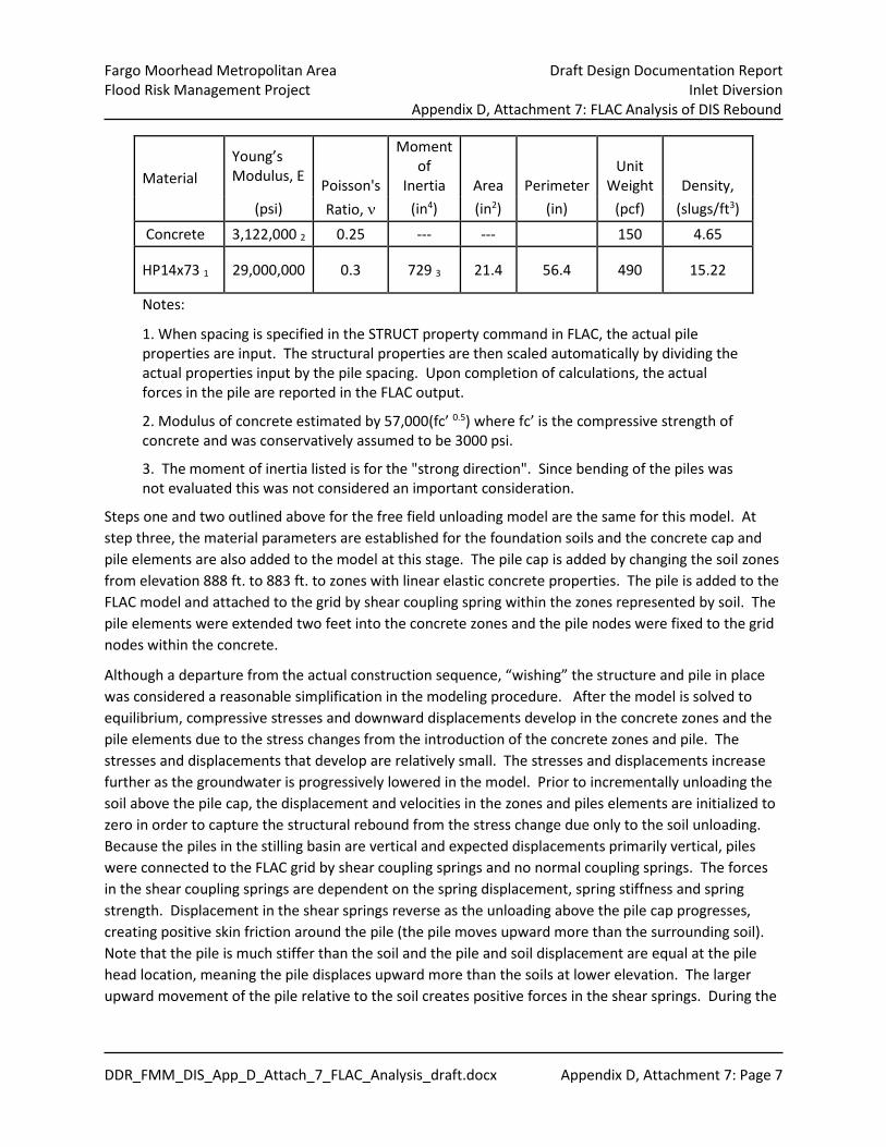
6.1. FLAC Modeling Procedure The same general procedure used for the free field unloading FLAC model was used simulate the loads and displacements expected to occur in the piles and pile cap of the stilling basin. Because the problem is dominated by excavation that produces significant reduction in vertical stress and subsequent expansion of the saturated fine-grained foundation soils, the stilling basin FLAC model was simplified to represent the center pile in the stilling basin pile layout with vertical boundaries set midway between the adjacent pile locations in the stilling basin. Figure 15 shows the location of the FLAC model in the stilling basin. Note that the pile spacing is 10 ft. in the direction of flow or the out-of-plane spacing in the FLAC model. The parameters used for the pile and concrete zones in FLAC are summarized in Error! Reference source not found.. The concrete was modelled as solid zones with linear elastic properties.



Material Young’s Modulus, E Poisson's

Moment of

Inertia Area Perimeter Unit

Weight Density, (psi) Ratio, ν (in4) (in2) (in) (pcf) (slugs/ft3)

Concrete 3,122,000 2 0.25 --- --- 150 4.65

HP14x73 1 29,000,000 0.3 729 3 21.4 56.4 490 15.22

Notes:

1. When spacing is specified in the STRUCT property command in FLAC, the actual pile properties are input. The structural properties are then scaled automatically by dividing the actual properties input by the pile spacing. Upon completion of calculations, the actual forces in the pile are reported in the FLAC output.

2. Modulus of concrete estimated by 57,000(fc’ 0.5) where fc’ is the compressive strength of concrete and was conservatively assumed to be 3000 psi.

3. The moment of inertia listed is for the "strong direction". Since bending of the piles was not evaluated this was not considered an important consideration.

Steps one and two outlined above for the free field unloading model are the same for this model. At step three, the material parameters are established for the foundation soils and the concrete cap and pile elements are also added to the model at this stage. The pile cap is added by changing the soil zones from elevation 888 ft. to 883 ft. to zones with linear elastic concrete properties. The pile is added to the FLAC model and attached to the grid by shear coupling spring within the zones represented by soil. The pile elements were extended two feet into the concrete zones and the pile nodes were fixed to the grid nodes within the concrete.

Although a departure from the actual construction sequence, “wishing” the structure and pile in place was considered a reasonable simplification in the modeling procedure. After the model is solved to equilibrium, compressive stresses and downward displacements develop in the concrete zones and the pile elements due to the stress changes from the introduction of the concrete zones and pile. The stresses and displacements that develop are relatively small. The stresses and displacements increase further as the groundwater is progressively lowered in the model. Prior to incrementally unloading the soil above the pile cap, the displacement and velocities in the zones and piles elements are initialized to zero in order to capture the structural rebound from the stress change due only to the soil unloading. Because the piles in the stilling basin are vertical and expected displacements primarily vertical, piles were connected to the FLAC grid by shear coupling springs and no normal coupling springs. The forces in the shear coupling springs are dependent on the spring displacement, spring stiffness and spring strength. Displacement in the shear springs reverse as the unloading above the pile cap progresses, creating positive skin friction around the pile (the pile moves upward more than the surrounding soil). Note that the pile is much stiffer than the soil and the pile and soil displacement are equal at the pile head location, meaning the pile displaces upward more than the soils at lower elevation. The larger upward movement of the pile relative to the soil creates positive forces in the shear springs. During the



unloading of the overburden soils, the relative shear spring displacements become large enough for the springs to yield and the full shear resistance of the pile in tension is realized.

6.2. Pile Elements

All the FLAC models assumed the same pile toe elevation of 836 ft. The pile elements were installed in one foot segments with the structural nodes spaced vertically each foot. Each one foot pile segment located within the soil zones are assigned geometric and mechanical properties. The geometric properties include the pile area, moment of inertia, and spacing. These properties are consistent along the entire pile length. The mechanical properties include the coupling spring parameters that will vary for each pile segment. The bottom shear coupling spring was not given any additional strength or altered spring stiffness to account for end bearing since the only interest was in the behavior of the pile due to the soil rebound. Two, one foot pile segments were located within the concrete zones and were fixed to the grid, meaning the structural nodes were linked or rigidly connected to the associated FLAC grid points

6.3. Pile-Soil Shear Coupling Springs Shear coupling springs connect the pile elements to the soil mesh and represent the axial shear transfer occurring between the pile and soil commonly termed skin friction. In FLAC, the soil-pile shear coupling springs are represented by a bi-linear model with a linear spring and a limiting shear force (elastic-plastic behavior). FLAC requires three input parameters for the shear coupling springs: cs_sstiff, cs_scoh, and cs_sfric. In the FLAC models, cs_sfric, the frictional component of the shear spring strength, was set to zero, and the limiting shear force was established by cs_scoh. The parameter cs_scoh is set to the long-term or drained shear strength between the soil-pile interface times the contact area. The long-term unit skin friction value 𝑓𝑓𝑠𝑠 in the foundation clays was established according to the equation:

𝑓𝑓𝑠𝑠 = 𝐾𝐾𝜎𝜎𝑣𝑣′ tan𝛿𝛿

Where 𝐾𝐾 = a lateral earth pressure coefficient 𝜎𝜎𝑣𝑣′ = effective overburden pressure

𝛿𝛿= friction angle between the soil and pile

The limiting value of the shear force that develops in the shear coupling spring was set according to:

cs_scoh = 𝑄𝑄𝑠𝑠 = 𝑓𝑓𝑠𝑠𝐴𝐴𝑠𝑠

𝑓𝑓𝑠𝑠 = long-term unit skin friction acting along the pile shaft 𝐴𝐴𝑠𝑠 = surface area of the pile shaft in contact with the soil

The determination of cs_sstiff and cs_scoh is described in the following section. The parameter cs_sstiff defines the stiffness of the shear spring. The effective overburden pressure,𝜎𝜎𝑣𝑣′ , used in the computation of the long-term unit skin friction was simply taken as the effective vertical stress computed from a geostatic calculation. In the case of the diversion channel excavation, this calculation was based on the accumulation of vertical stress from a unit depth times the effective unit weight of soil determined from the final excavated elevation. The effective vertical stress around the pile is expected to decrease over



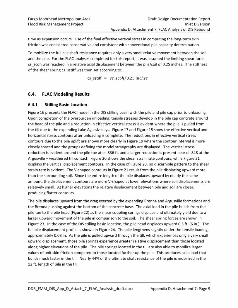
time as expansion occurs. Use of the final effective vertical stress in computing the long-term skin friction was considered conservative and consistent with conventional pile capacity determination.

To mobilize the full pile shaft resistance requires only a very small relative movement between the soil and the pile. For the FLAC analyses completed for this report, it was assumed the limiting shear force cs_scoh was reached in a relative axial displacement between the pile/soil of 0.25 inches. The stiffness of the shear spring cs_sstiff was then set according to:

cs_sstiff = 𝑐𝑐𝑠𝑠_𝑠𝑠𝑐𝑐𝑠𝑠ℎ 0.25 𝑠𝑠𝑠𝑠𝑐𝑐ℎ𝑒𝑒𝑠𝑠⁄

6.4. FLAC Modeling Results

6.4.1 Stilling Basin Location

Figure 16 presents the FLAC model in the DIS stilling basin with the pile and pile cap prior to unloading. Upon completion of the overburden unloading, tensile stresses develop in the pile cap concrete around the head of the pile and a reduction in effective vertical stress is evident where the pile is pulled from the till due to the expanding Lake Agassiz clays. Figure 17 and Figure 18 show the effective vertical and horizontal stress contours after unloading is complete. The reductions in effective vertical stress contours due to the pile uplift are shown more clearly in Figure 19 where the contour interval is more closely spaced and the groups defining the model stratigraphy are displayed. The vertical stress reduction is evident around the pile toe at el. 836 ft. and a larger reduction is present near el. 848 at the Argusville – weathered till contact. Figure 20 shows the shear strain rate contours, while Figure 21 displays the vertical displacement contours. In the case of Figure 20, no discernible pattern to the shear strain rate is evident. The V-shaped contours in Figure 21 result from the pile displacing upward more than the surrounding soil. Since the entire length of the pile displaces upward by nearly the same amount, the displacement contours are more V-shaped at lower elevations where soil displacements are relatively small. At higher elevations the relative displacement between pile and soil are closer, producing flatter contours.

The pile displaces upward from the drag exerted by the expanding Brenna and Argusville formations and the Brenna pushing against the bottom of the concrete base. The axial load in the pile builds from the pile toe to the pile head (Figure 22) as the shear coupling springs displace and ultimately yield due to a larger upward movement of the pile in comparison to the soil. The shear spring forces are shown in Figure 23. In the case of the DIS stilling basin location, the pile head displaces upward 0.5 ft. (6 in.). The full pile displacement profile is shown in Figure 24. The pile lengthens slightly under the tensile loading, approximately 0.08 in. As the pile is pulled upward through the till, which experiences only a very small upward displacement, those pile springs experience greater relative displacement than those located along higher elevations of the pile. The pile springs located in the till are also able to mobilize larger values of unit skin friction compared to those located further up the pile. This produces axial load that builds much faster in the till. Nearly 44% of the ultimate shaft resistance of the pile is mobilized in the 12 ft. length of pile in the till.



6.4.2 Shear Transfer in the Till

The shear transfer between soil-pile in the weathered and intact till is an important consideration. The unit skin friction is determined from𝑓𝑓𝑠𝑠 = 𝐾𝐾𝜎𝜎𝑣𝑣′ tan𝛿𝛿, where 𝐾𝐾 tan 𝛿𝛿 is often replaced by the coefficient 𝛽𝛽 giving the familiar𝑓𝑓𝑠𝑠 = 𝛽𝛽𝜎𝜎𝑣𝑣′ . In soft clays 𝛽𝛽 normally varies between 0.2 and 0.4. In the Lake Agassiz clays, a 𝛽𝛽 value of 0.3 was used to determine the unit skin friction value. Initially the same 𝛽𝛽 value was applied to both till formations. As a check, the 𝛽𝛽value in the till was increased from 0.3 to 0.4. This change increases the available shear transfer of the pile to the surrounding till. A comparison from the FLAC results is shown in Table 2. Clearly the available shear transfer between pile-till is an important consideration given the effect on the structural rebound and the load transferred into the pile cap.

Table 2 Comparison of Axial Load and Displacement for Varying 𝛽𝛽 Values in the Till (Stilling Basin Location)

𝛽𝛽 Value in the Till

Axial Load at Pile Head following Unloading (kips)

Axial Displacement at Pile Head following Unloading (inches)

0.3 67.4 6

0.4 77.5 3.7

A higher unit skin friction value in the till translates to less pile displacement and more tensile load in the pile. The till serves as an anchoring material and the length of embedded pile as the anchoring length. Additional numerical modeling indicated increasing the length of the pile by further embedment into the till effectively reduced the upward displacement at the pile head, while increasing the tensile loads in the pile. While embedding the pile further into the till is a simple change in a numerical model, as a practical consideration, H piles cannot be driven very far into a soil with SPT blow counts of 100 or more.

6.4.3 Approach Apron

A FLAC model representative of the DIS approach apron was also analyzed. The model was setup in the same manner as the stilling basin model with a single pile spaced 10 ft. on center in the upstream direction and model side boundaries set at the line of symmetry between piles 5 ft. either side of the pile (Figure 25). The primary difference between the approach apron and stilling basin model is the pile cap is located at a higher elevation 899 ft. compared to 888 ft. in the stilling basin. This means 11 ft. less overburden removal and a pile that’s also 11 ft. longer since the assumed pile toe el. of 836 ft. did not change. The approach apron slab in the FLAC model was 3 ft. thick compared to 5 ft. in the stilling basin. The FLAC model after removal of the overburden is shown in Figure 26. Due to the higher invert elevation at the approach apron, the effective overburden pressure is greater at this location resulting in higher unit skin friction values so the pile shear coupling spring parameters were set accordingly.

Figure 27 and Figure 28 show the effective vertical and horizontal stress contours after unloading is complete. Reductions in effective vertical stress are again evident around the pile toe at el. 836 ft. and near el. 848 at the Argusville – weathered till contact. Figure 29 shows the reduction in effective vertical stress as line contours at a 50 psf contour interval overlaid on the material groups. Figure 30 displays



the shear strain rate contours. This figure clearly shows the shear transfer from the pile to the surrounding soil as the pile is pulled from the weathered till. Figure 31 shows the vertical displacement contours with the pile displacing upward more than the surrounding soil.

The axial load in the pile builds from the pile toe to the pile head (Figure 32) with a maximum tension force at the pile head of 123.5 kips. The shear spring forces are shown in Figure 33. The shear spring forces are larger at the approach apron location than the stilling basin (Figure 23) due to the higher available unit skin friction. The pile displacement profile is shown in Figure 34. The pile head displacement was 0.204 ft. (2.4 in.). A summary of the pile head displacements and axial loads is provided in Table 3 for both the stilling basin and approach apron models, as well as the two different beta values used to estimate the unit skin friction in the till.

Table 3 Comparison of Axial Load and Displacement for Varying 𝛽𝛽 Values in the Till (Stilling Basin and

Approach Apron Locations)

Model Location

𝛽𝛽 Value in the Till

Axial Load at Pile Head following Unloading (kips)

Axial Displacement at Pile Head following Unloading (inches)

Stilling Basin 0.3 67.4 6

Stilling Basin 0.4 77.5 3.7

Approach Apron 0.3 123.5 2.4

Approach Apron 0.4 129.5 1.6

6.4.4 Control Structure

A two dimensional FLAC model of the control structure slab was also analyzed. The cross-section (Figure 35) was located at an abutment pier location and assumed vertical piles for the entire section. Note that the pile layout beneath the control structure generally includes vertical piles under the piers and rows of batter piles aligned either upstream or downstream that alternate direction every row or two between the piers. A two dimensional plane strain model of the control structure slab taken perpendicular to the direction of flow was considered a conservative assumption. The additional conservatism of not including the center vertical pile under the pier location to match the batter pile layout was considered reasonable. Figure 36 shows the FLAC model section including the grid, material groups, pile locations, and boundary conditions. The cross-section includes 10 piles, five located under the stepped spillway and five located under the upstream half of the horizontal slab. The piles were fixed to the FLAC grid for the two foot embedment into the concrete slab. The slab thickness was 6 ft. at the upstream model limit and 7 ft. at the downstream model limit. The modeling steps for the control structure were the same as the stilling basin and approach apron models that included a single pile and pile cap.



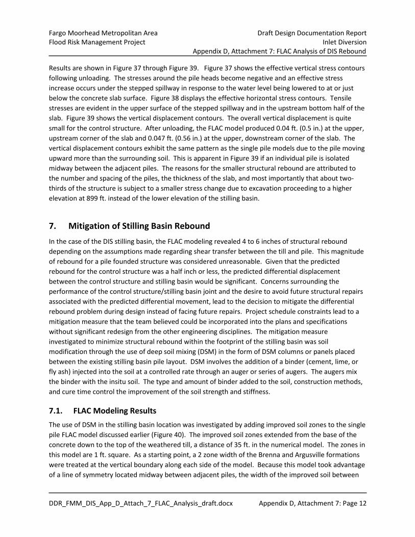
Results are shown in Figure 37 through Figure 39. Figure 37 shows the effective vertical stress contours following unloading. The stresses around the pile heads become negative and an effective stress increase occurs under the stepped spillway in response to the water level being lowered to at or just below the concrete slab surface. Figure 38 displays the effective horizontal stress contours. Tensile stresses are evident in the upper surface of the stepped spillway and in the upstream bottom half of the slab. Figure 39 shows the vertical displacement contours. The overall vertical displacement is quite small for the control structure. After unloading, the FLAC model produced 0.04 ft. (0.5 in.) at the upper, upstream corner of the slab and 0.047 ft. (0.56 in.) at the upper, downstream corner of the slab. The vertical displacement contours exhibit the same pattern as the single pile models due to the pile moving upward more than the surrounding soil. This is apparent in Figure 39 if an individual pile is isolated midway between the adjacent piles. The reasons for the smaller structural rebound are attributed to the number and spacing of the piles, the thickness of the slab, and most importantly that about two-thirds of the structure is subject to a smaller stress change due to excavation proceeding to a higher elevation at 899 ft. instead of the lower elevation of the stilling basin.

7. Mitigation of Stilling Basin Rebound In the case of the DIS stilling basin, the FLAC modeling revealed 4 to 6 inches of structural rebound depending on the assumptions made regarding shear transfer between the till and pile. This magnitude of rebound for a pile founded structure was considered unreasonable. Given that the predicted rebound for the control structure was a half inch or less, the predicted differential displacement between the control structure and stilling basin would be significant. Concerns surrounding the performance of the control structure/stilling basin joint and the desire to avoid future structural repairs associated with the predicted differential movement, lead to the decision to mitigate the differential rebound problem during design instead of facing future repairs. Project schedule constraints lead to a mitigation measure that the team believed could be incorporated into the plans and specifications without significant redesign from the other engineering disciplines. The mitigation measure investigated to minimize structural rebound within the footprint of the stilling basin was soil modification through the use of deep soil mixing (DSM) in the form of DSM columns or panels placed between the existing stilling basin pile layout. DSM involves the addition of a binder (cement, lime, or fly ash) injected into the soil at a controlled rate through an auger or series of augers. The augers mix the binder with the insitu soil. The type and amount of binder added to the soil, construction methods, and cure time control the improvement of the soil strength and stiffness.

7.1. FLAC Modeling Results The use of DSM in the stilling basin location was investigated by adding improved soil zones to the single pile FLAC model discussed earlier (Figure 40). The improved soil zones extended from the base of the concrete down to the top of the weathered till, a distance of 35 ft. in the numerical model. The zones in this model are 1 ft. square. As a starting point, a 2 zone width of the Brenna and Argusville formations were treated at the vertical boundary along each side of the model. Because this model took advantage of a line of symmetry located midway between adjacent piles, the width of the improved soil between



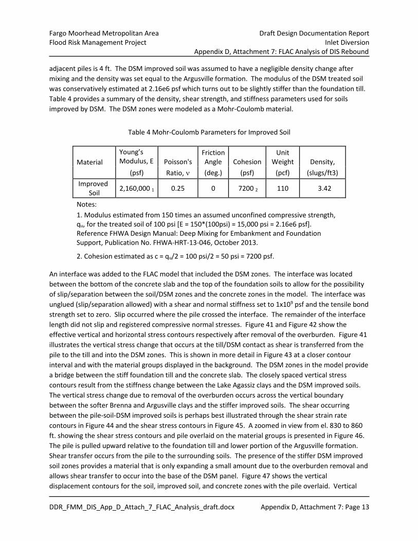
adjacent piles is 4 ft. The DSM improved soil was assumed to have a negligible density change after mixing and the density was set equal to the Argusville formation. The modulus of the DSM treated soil was conservatively estimated at 2.16e6 psf which turns out to be slightly stiffer than the foundation till. Table 4 provides a summary of the density, shear strength, and stiffness parameters used for soils improved by DSM. The DSM zones were modeled as a Mohr-Coulomb material.

Table 4 Mohr-Coulomb Parameters for Improved Soil

Material Young’s Modulus, E Poisson's

Friction Angle Cohesion

Unit Weight Density,

(psf) Ratio, ν (deg.) (psf) (pcf) (slugs/ft3) Improved

Soil 2,160,000 1 0.25 0 7200 2 110 3.42

Notes: 1. Modulus estimated from 150 times an assumed unconfined compressive strength, qu, for the treated soil of 100 psi [E = 150*(100psi) = 15,000 psi = 2.16e6 psf]. Reference FHWA Design Manual: Deep Mixing for Embankment and Foundation Support, Publication No. FHWA-HRT-13-046, October 2013.

2. Cohesion estimated as c = qu/2 = 100 psi/2 = 50 psi = 7200 psf.

An interface was added to the FLAC model that included the DSM zones. The interface was located between the bottom of the concrete slab and the top of the foundation soils to allow for the possibility of slip/separation between the soil/DSM zones and the concrete zones in the model. The interface was unglued (slip/separation allowed) with a shear and normal stiffness set to 1x109 psf and the tensile bond strength set to zero. Slip occurred where the pile crossed the interface. The remainder of the interface length did not slip and registered compressive normal stresses. Figure 41 and Figure 42 show the effective vertical and horizontal stress contours respectively after removal of the overburden. Figure 41 illustrates the vertical stress change that occurs at the till/DSM contact as shear is transferred from the pile to the till and into the DSM zones. This is shown in more detail in Figure 43 at a closer contour interval and with the material groups displayed in the background. The DSM zones in the model provide a bridge between the stiff foundation till and the concrete slab. The closely spaced vertical stress contours result from the stiffness change between the Lake Agassiz clays and the DSM improved soils. The vertical stress change due to removal of the overburden occurs across the vertical boundary between the softer Brenna and Argusville clays and the stiffer improved soils. The shear occurring between the pile-soil-DSM improved soils is perhaps best illustrated through the shear strain rate contours in Figure 44 and the shear stress contours in Figure 45. A zoomed in view from el. 830 to 860 ft. showing the shear stress contours and pile overlaid on the material groups is presented in Figure 46. The pile is pulled upward relative to the foundation till and lower portion of the Argusville formation. Shear transfer occurs from the pile to the surrounding soils. The presence of the stiffer DSM improved soil zones provides a material that is only expanding a small amount due to the overburden removal and allows shear transfer to occur into the base of the DSM panel. Figure 47 shows the vertical displacement contours for the soil, improved soil, and concrete zones with the pile overlaid. Vertical



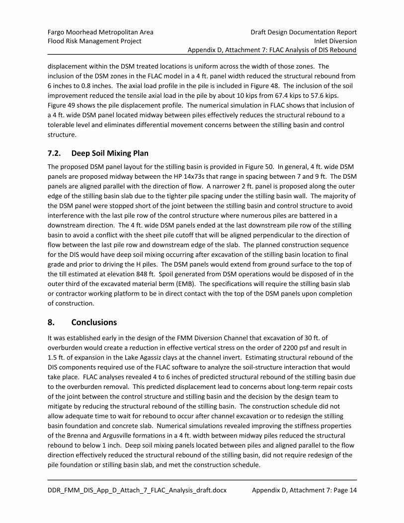
displacement within the DSM treated locations is uniform across the width of those zones. The inclusion of the DSM zones in the FLAC model in a 4 ft. panel width reduced the structural rebound from 6 inches to 0.8 inches. The axial load profile in the pile is included in Figure 48. The inclusion of the soil improvement reduced the tensile axial load in the pile by about 10 kips from 67.4 kips to 57.6 kips. Figure 49 shows the pile displacement profile. The numerical simulation in FLAC shows that inclusion of a 4 ft. wide DSM panel located midway between piles effectively reduces the structural rebound to a tolerable level and eliminates differential movement concerns between the stilling basin and control structure.

7.2. Deep Soil Mixing Plan The proposed DSM panel layout for the stilling basin is provided in Figure 50. In general, 4 ft. wide DSM panels are proposed midway between the HP 14x73s that range in spacing between 7 and 9 ft. The DSM panels are aligned parallel with the direction of flow. A narrower 2 ft. panel is proposed along the outer edge of the stilling basin slab due to the tighter pile spacing under the stilling basin wall. The majority of the DSM panel were stopped short of the joint between the stilling basin and control structure to avoid interference with the last pile row of the control structure where numerous piles are battered in a downstream direction. The 4 ft. wide DSM panels ended at the last downstream pile row of the stilling basin to avoid a conflict with the sheet pile cutoff that will be aligned perpendicular to the direction of flow between the last pile row and downstream edge of the slab. The planned construction sequence for the DIS would have deep soil mixing occurring after excavation of the stilling basin location to final grade and prior to driving the H piles. The DSM panels would extend from ground surface to the top of the till estimated at elevation 848 ft. Spoil generated from DSM operations would be disposed of in the outer third of the excavated material berm (EMB). The specifications will require the stilling basin slab or contractor working platform to be in direct contact with the top of the DSM panels upon completion of construction.

8. Conclusions

It was established early in the design of the FMM Diversion Channel that excavation of 30 ft. of overburden would create a reduction in effective vertical stress on the order of 2200 psf and result in 1.5 ft. of expansion in the Lake Agassiz clays at the channel invert. Estimating structural rebound of the DIS components required use of the FLAC software to analyze the soil-structure interaction that would take place. FLAC analyses revealed 4 to 6 inches of predicted structural rebound of the stilling basin due to the overburden removal. This predicted displacement lead to concerns about long-term repair costs of the joint between the control structure and stilling basin and the decision by the design team to mitigate by reducing the structural rebound of the stilling basin. The construction schedule did not allow adequate time to wait for rebound to occur after channel excavation or to redesign the stilling basin foundation and concrete slab. Numerical simulations revealed improving the stiffness properties of the Brenna and Argusville formations in a 4 ft. width between midway piles reduced the structural rebound to below 1 inch. Deep soil mixing panels located between piles and aligned parallel to the flow direction effectively reduced the structural rebound of the stilling basin, did not require redesign of the pile foundation or stilling basin slab, and met the construction schedule.



9. References

Reese, Lymon C., et al. Computer Program APile Plus Version 4.0 Technical Manual. Austin, Texas.

2004.

Terzaghi, K., Peck, R. B., & Mesri, G. (1996). Soil Mechanics in Engineering Practice. New York: John Wiley

& Sons, Inc.

U.S. Army Corps of Engineers. EM 1110‐2‐2906, Design of Pile Foundations. Washington DC. January 15, 1991.

U.S. Army Corps of Engineers, St. Paul District. General Report: Geotechnical Design and Geology of the

Fargo‐Moorhead Metropolitan Area Flood Risk Management Project North Dakota Diversion

Alignment. St. Paul, MN. May 13, 2013.

U.S. Army Corps of Engineers, St. Paul District. Appendix D, Attachment 6: FLAC Analysis of Floodwall,

Fargo Moorhead Metropolitan Area Flood Risk Management Project, Draft Design

Documentation Report. January 26, 2016 (Doc. Version).

U.S. Army Corps of Engineers, St. Paul District. Appendix D, Attachment 1: Settlement Calculations,

Fargo Moorhead Metropolitan Area Flood Risk Management Project, 90% Design

Documentation Report. July 2015.

U.S. Department of Transportation, Federal Highway Administration. Publication No. FHWA_HRT‐13‐

046, Federal Highway Administration Design Manual: Deep Mixing for Embankment and

Foundation Support. Washington DC. October 2013.

Wood, D. M. (1990). Soil Behavior and Critical State Soil Mechanics. New York: Cambridge University

Press.

10. District Quality Control

A district quality control (DQC) review of this report and the associated FLAC files was completed by the

undersigned. The review included checks of the model inputs, the procedures followed to set up the

model states, and the overall validity of the modeling and reported results.

Figure 1 Plan View of Diversion Inlet Apppendix D, Attachment 7: Page 16

Figure 2 Profile of Diversion Channel, Structure, and Connecting Channel

Apppendix D, Attachment 7: Page 17

Figure 3 Boring Log 15-233M


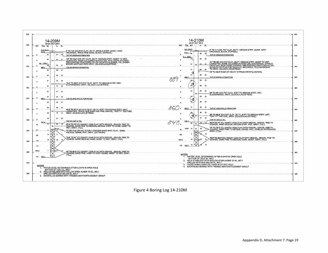
Figure 4 Boring Log 14-210M


Figure 5 Determination of Reference Specific Volume and Preconsolidation Pressure for the Argusville Fm.

CIU Triaxial Test Results Argusville Formation

Consolidation Void Ratio ReferenceSoil Boring Sample Depth Pressure after Initial Specific

Formation No. No. (ft) (tsf) Consolidation Void Ratio Volume

Argusville 11-119MU 3 50-52 2.92 1.0205 1.0645 4.8824211-107MU 3 40-42 2.94 0.9527 0.9695 4.81687311-110MU 4 55-57 2.96 1.3326 1.3705 5.1990110-79MU 2 40-42 3.00 1.14 1.31 5.0108411-119MU 2 40-42 3.00 1.0402 1.08 4.9110411-118MU 3 45-47 3.02 1.3292 1.3543 5.20223310-105MU 4 45-47 3.04 1.6774 1.7065 5.55261111-110MU 5 60-62 3.97 1.1821 1.2297 5.14539110-80MU 3 55-57 4.00 1.21 1.45 5.17577511-118MU 4 55-57 4.01 1.2029 1.2387 5.16949911-118MU 5 65-67 4.01 1.0046 1.0482 4.97119911-107MU 4 50-52 4.04 0.9777 1.0099 4.946759

Average (all) 3.41 1.17 1.24 5.08

pc'sigmav max Ko sigmah max pmax qmax M pc0

7200 0.8 5760 6240 1440 0.61 7133


Figure 6 Determination of Reference Specific Volume and Preconsolidation Pressure for the Brenna Fm.

CIU Triaxial Test Results Brenna Formation

Consolidation Void Ratio ReferenceSoil Boring Sample Depth Pressure after Initial Specific

Formation No. No. (ft) (tsf) Consolidation Void Ratio Volume

Brenna 11-110MU 2 35-37 1.98 1.0163 1.038 4.7500210-105MU 2 25-27 2.00 1.5732 1.5926 5.31023610-105MU 3 35-37 2.00 1.7000 1.7000 5.43703611-118MU 2 33-35 2.00 1.1193 1.1307 4.85633611-119MU 1 30-32 2.02 1.0773 1.0998 4.8176211-107MU 2 30-32 2.03 1.1423 1.1538 4.8842509-14MU 2 15-17 2.80 2.0787 2.4393 5.92677209-25MU 4 38-40 2.99 1.8783 1.8783 5.74803811-110MU 3 48-50 3.05 1.4494 1.5165 5.32569511-107MU 1 20-22 3.14 1.2616 1.286 5.14749109-25MU 5 68-70 3.89 1.4744 1.4744 5.43097309-11MU 2 30-32 3.97 1.5197 1.6308 5.48299109-25MU 4 50-52 3.99 1.6191 1.7353 5.58404910-78MU 2 25-27 4.00 1.01 1.27 4.97577510-80MU 2 35-37 4.00 1.17 1.36 5.13577509-11MU 3 40-42 4.00 1.4482 1.5562 5.41397509-26MU 3 28-30 4.01 1.4349 1.5425 5.40149909-27MU 3 32-34 4.01 1.7999 1.9886 5.76649909-27MU 4 64-66 4.01 1.2568 1.3827 5.22339909-53MU 2 28-30 4.02 1.7365 1.8265 5.703921

Average (all) 3.20 1.44 1.53 5.32

pc'sigmav max Ko sigmah max pmax qmax M pc0

6400 0.94 6016 6144 384 0.49 6244


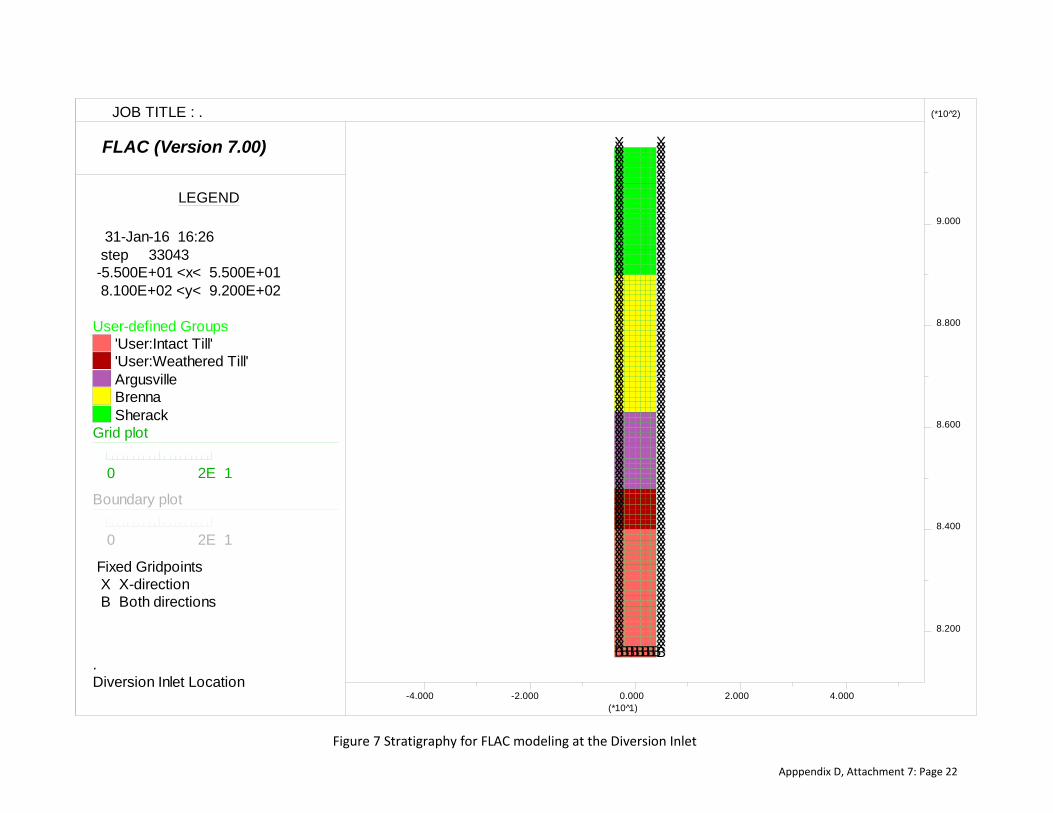
Figure 7 Stratigraphy for FLAC modeling at the Diversion Inlet

FLAC (Version 7.00)

LEGEND

31-Jan-16 16:26 step 33043 -5.500E+01 <x< 5.500E+01 8.100E+02 <y< 9.200E+02

User-defined Groups'User:Intact Till''User:Weathered Till'ArgusvilleBrennaSherack

Grid plot

0 2E 1

Boundary plot

0 2E 1

Fixed Gridpoints

BXXXXXXXXXXXXXXXXXXXXXXXXXXXXXXXXXXXXXXXXXXXXXXXXXXXXXXXXXXXXXXXXXXXXXXXXXXXXXXXXXXXXXXXXXXXXXXXXXXXX

BBBBBBBBXXXXXXXXXXXXXXXXXXXXXXXXXXXXXXXXXXXXXXXXXXXXXXXXXXXXXXXXXXXXXXXXXXXXXXXXXXXXXXXXXXXXXXXXXXXXXXXXXXXX

X X-direction B Both directions

8.200

8.400

8.600

8.800

9.000

(*10 2̂)

-4.000 -2.000 0.000 2.000 4.000(*10 1̂)

JOB TITLE : .

.Diversion Inlet Location


Figure 8 Effective Vertical Stress Contours for Insitu Conditions

FLAC (Version 7.00)

LEGEND

1-Feb-16 15:28 step 3119 -5.500E+01 <x< 5.500E+01 8.100E+02 <y< 9.200E+02

Effec. SYY-Stress Contours -5.00E+03 -4.00E+03 -3.00E+03 -2.00E+03 -1.00E+03 0.00E+00

Contour interval= 1.00E+03Extrap. by averagingPile plot

8.200

8.400

8.600

8.800

9.000

(*10^2)

-4.000 -2.000 0.000 2.000 4.000(*10^1)

JOB TITLE : .



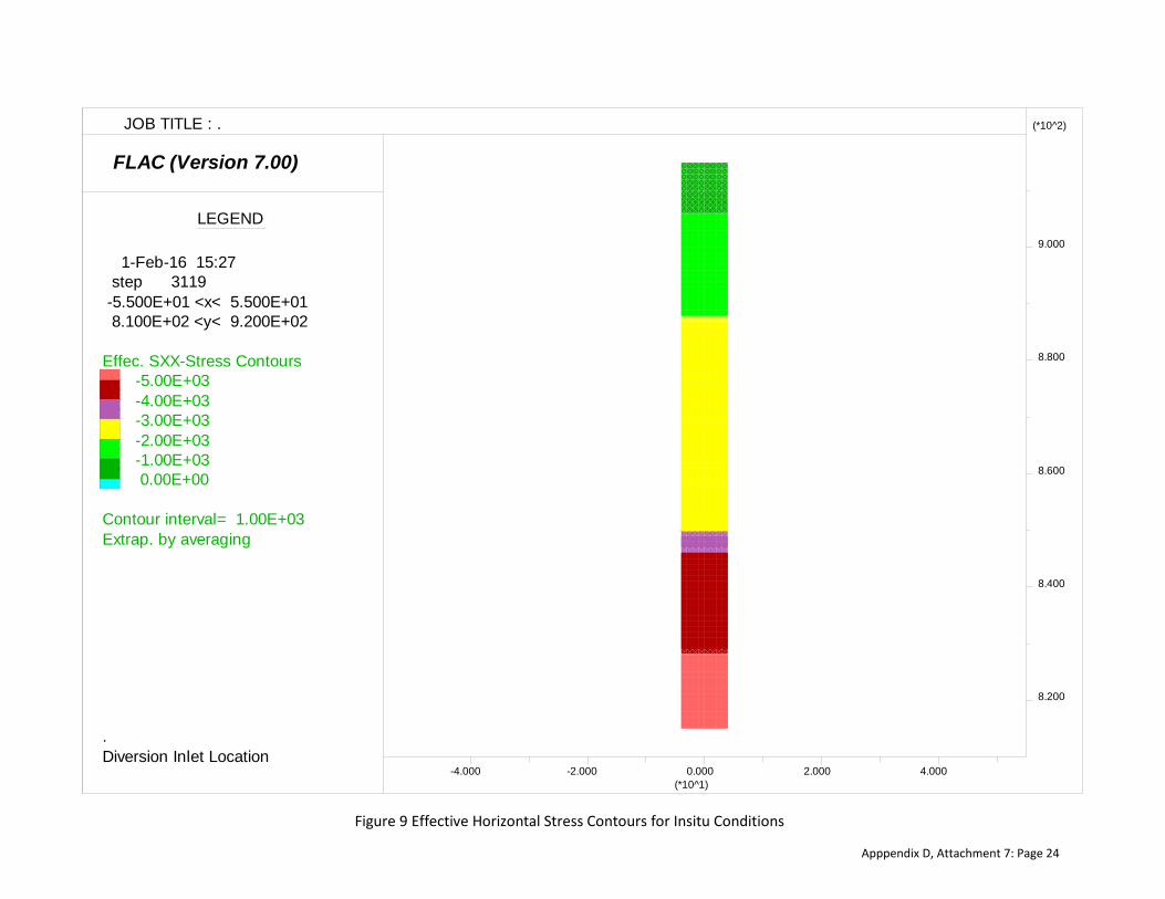
Figure 9 Effective Horizontal Stress Contours for Insitu Conditions

FLAC (Version 7.00)

LEGEND

1-Feb-16 15:27 step 3119 -5.500E+01 <x< 5.500E+01 8.100E+02 <y< 9.200E+02

Effec. SXX-Stress Contours -5.00E+03 -4.00E+03 -3.00E+03 -2.00E+03 -1.00E+03 0.00E+00

Contour interval= 1.00E+03Extrap. by averaging

8.200

8.400

8.600

8.800

9.000

(*10^2)

-4.000 -2.000 0.000 2.000 4.000(*10^1)

JOB TITLE : .



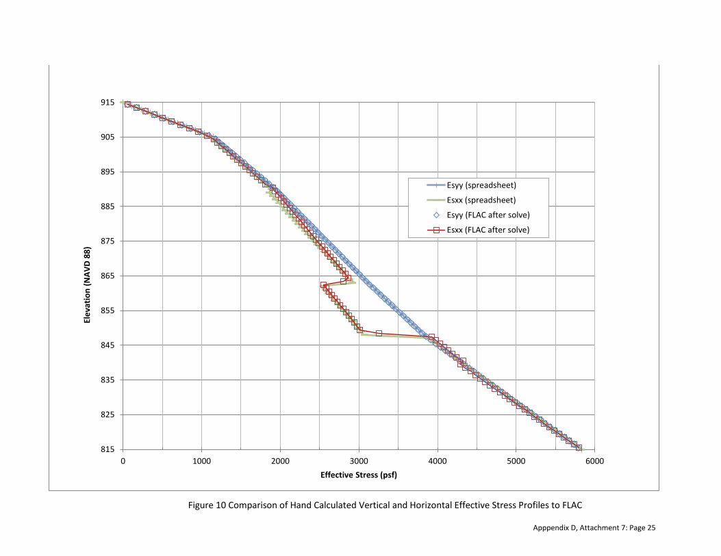
Figure 10 Comparison of Hand Calculated Vertical and Horizontal Effective Stress Profiles to FLAC

815

825

835

845

855

865

875

885

895

905

915

0 1000 2000 3000 4000 5000 6000

Elev

atio

n (N

AVD

88)

Effective Stress (psf)

Esyy (spreadsheet)

Esxx (spreadsheet)

Esyy (FLAC after solve)

Esxx (FLAC after solve)


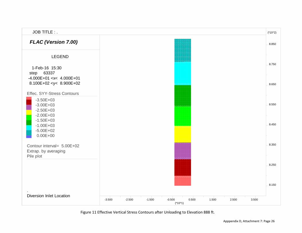
Figure 11 Effective Vertical Stress Contours after Unloading to Elevation 888 ft.

FLAC (Version 7.00)

LEGEND

1-Feb-16 15:30 step 63337 -4.000E+01 <x< 4.000E+01 8.100E+02 <y< 8.900E+02

Effec. SYY-Stress Contours -3.50E+03 -3.00E+03 -2.50E+03 -2.00E+03 -1.50E+03 -1.00E+03 -5.00E+02 0.00E+00


8.150

8.250

8.350

8.450

8.550

8.650

8.750

8.850

(*10^2)

-3.500 -2.500 -1.500 -0.500 0.500 1.500 2.500 3.500(*10^1)

JOB TITLE : .



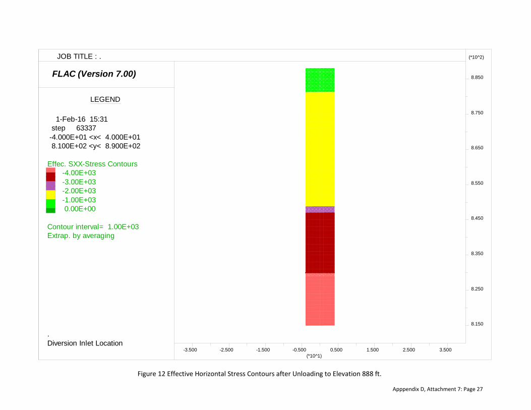
Figure 12 Effective Horizontal Stress Contours after Unloading to Elevation 888 ft.

FLAC (Version 7.00)

LEGEND

1-Feb-16 15:31 step 63337 -4.000E+01 <x< 4.000E+01 8.100E+02 <y< 8.900E+02

Effec. SXX-Stress Contours -4.00E+03 -3.00E+03 -2.00E+03 -1.00E+03 0.00E+00

Contour interval= 1.00E+03Extrap. by averaging

8.150

8.250

8.350

8.450

8.550

8.650

8.750

8.850

(*10^2)

-3.500 -2.500 -1.500 -0.500 0.500 1.500 2.500 3.500(*10^1)

JOB TITLE : .



Figure 13 Vertical Displacement Contours after Unloading to Elevation 888 ft.

FLAC (Version 7.00)

LEGEND

1-Feb-16 15:33 step 63337 -4.000E+01 <x< 4.000E+01 8.100E+02 <y< 8.900E+02

Y-displacement contours 0.00E+00 2.00E-01 4.00E-01 6.00E-01 8.00E-01 1.00E+00 1.20E+00Contour interval= 1.00E-01

8.150

8.250

8.350

8.450

8.550

8.650

8.750

8.850

(*10^2)

-3.500 -2.500 -1.500 -0.500 0.500 1.500 2.500 3.500(*10^1)

JOB TITLE : .



Figure 14 Rebound Profile Comparison of FLAC to One Dimensional Expansion Spreadsheet Calculation


Figure 15 Location of the Single Pile FLAC Model in the DIS Stilling Basin


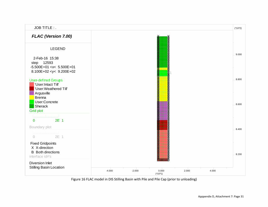
Figure 16 FLAC model in DIS Stilling Basin with Pile and Pile Cap (prior to unloading)

FLAC (Version 7.00)

LEGEND

2-Feb-16 15:38 step 12593 -5.500E+01 <x< 5.500E+01 8.100E+02 <y< 9.200E+02

User-defined Groups'User:Intact Till''User:Weathered Till'ArgusvilleBrennaUser:ConcreteSherack

Grid plot

0 2E 1

Boundary plot

0 2E 1

Fixed Gridpoints

BXXXXXXXXXXXXXXXXXXXXXXXXXXXXXXXXXXXXXXXXXXXXXXXXXXXXXXXXXXXXXXXXXXXXXXXXXXXXXXXXXXXXXXXXXXXXXXXXXXXX

BBBBBBBBXXXXXXXXXXXXXXXXXXXXXXXXXXXXXXXXXXXXXXXXXXXXXXXXXXXXXXXXXXXXXXXXXXXXXXXXXXXXXXXXXXXXXXXXXXXXXXXXXXXX

X X-direction B Both directionsinterface id#'s

1

8.200

8.400

8.600

8.800

9.000

(*10 2̂)

-4.000 -2.000 0.000 2.000 4.000(*10 1̂)

JOB TITLE : .

Diversion InletStilling Basin Location


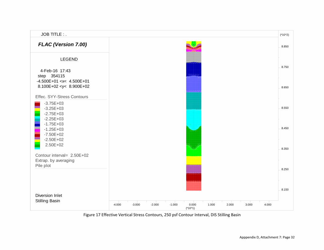
Figure 17 Effective Vertical Stress Contours, 250 psf Contour Interval, DIS Stilling Basin

FLAC (Version 7.00)

LEGEND

4-Feb-16 17:43 step 354115 -4.500E+01 <x< 4.500E+01 8.100E+02 <y< 8.900E+02

Effec. SYY-Stress Contours -3.75E+03 -3.25E+03 -2.75E+03 -2.25E+03 -1.75E+03 -1.25E+03 -7.50E+02 -2.50E+02 2.50E+02


8.150

8.250

8.350

8.450

8.550

8.650

8.750

8.850

(*10^2)

-4.000 -3.000 -2.000 -1.000 0.000 1.000 2.000 3.000 4.000(*10^1)

JOB TITLE : .

Diversion InletStilling Basin


Figure 18 Effective Horizontal Stress Contours, 250 psf Contour Interval, DIS Stilling Basin

FLAC (Version 7.00)

LEGEND

4-Feb-16 17:43 step 354115 -4.500E+01 <x< 4.500E+01 8.100E+02 <y< 8.900E+02

Effec. SXX-Stress Contours -5.00E+03 -4.50E+03 -4.00E+03 -3.50E+03 -3.00E+03 -2.50E+03 -2.00E+03 -1.50E+03 -1.00E+03


8.150

8.250

8.350

8.450

8.550

8.650

8.750

8.850

(*10^2)

-4.000 -3.000 -2.000 -1.000 0.000 1.000 2.000 3.000 4.000(*10^1)

JOB TITLE : .



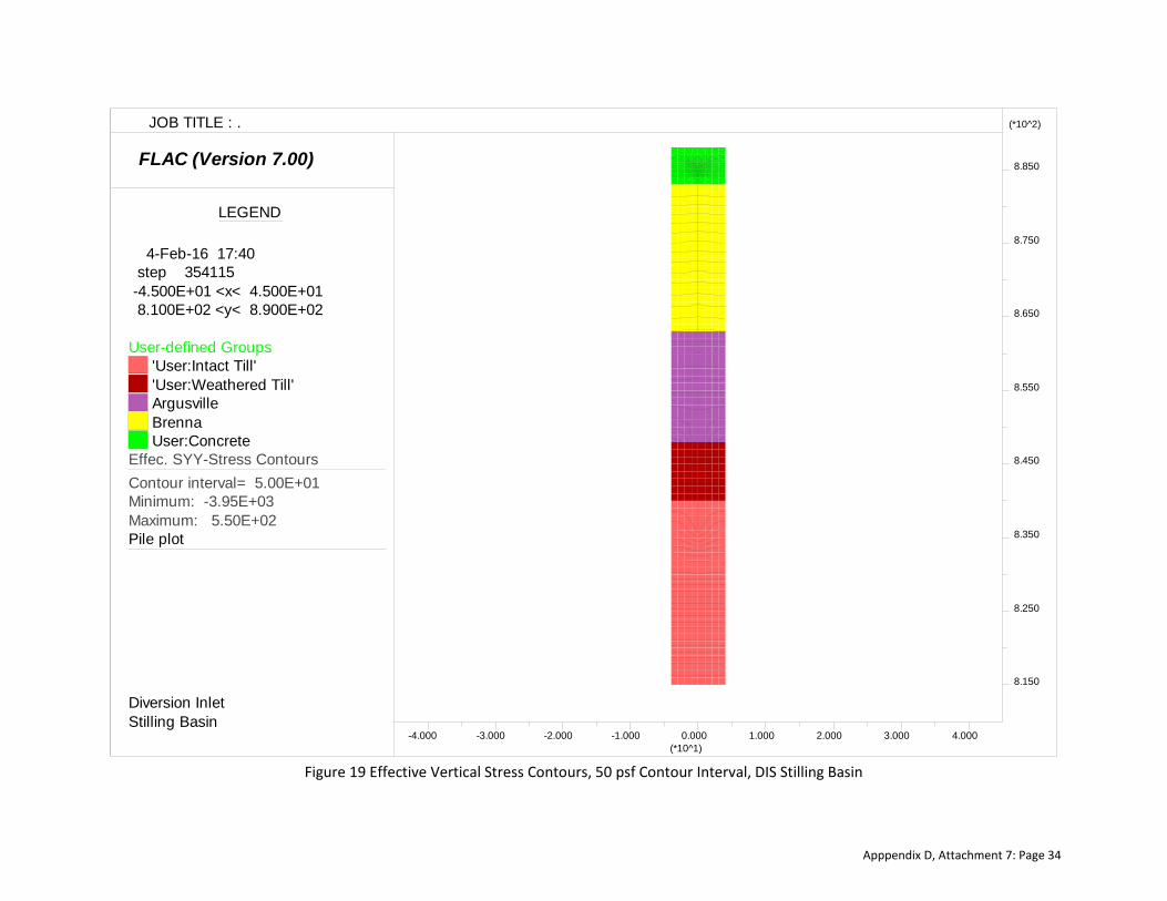
Figure 19 Effective Vertical Stress Contours, 50 psf Contour Interval, DIS Stilling Basin

FLAC (Version 7.00)

LEGEND

4-Feb-16 17:40 step 354115 -4.500E+01 <x< 4.500E+01 8.100E+02 <y< 8.900E+02

User-defined Groups'User:Intact Till''User:Weathered Till'ArgusvilleBrennaUser:Concrete

Effec. SYY-Stress ContoursContour interval= 5.00E+01Minimum: -3.95E+03Maximum: 5.50E+02Pile plot

8.150

8.250

8.350

8.450

8.550

8.650

8.750

8.850

(*10^2)

-4.000 -3.000 -2.000 -1.000 0.000 1.000 2.000 3.000 4.000(*10^1)

JOB TITLE : .



Figure 20 Shear Strain Rate Contours, DIS Stilling Basin

FLAC (Version 7.00)

LEGEND

4-Feb-16 17:39 step 354115 -4.500E+01 <x< 4.500E+01 8.100E+02 <y< 8.900E+02

Max. shear strain-rate 0.00E+00 5.00E-09 1.00E-08 1.50E-08 2.00E-08 2.50E-08 3.00E-08 3.50E-08 4.00E-08

Contour interval= 5.00E-09Extrap. by averagingGrid plot

0 2E 1

Pile plot 8.150

8.250

8.350

8.450

8.550

8.650

8.750

8.850

(*10^2)

-4.000 -3.000 -2.000 -1.000 0.000 1.000 2.000 3.000 4.000(*10^1)

JOB TITLE : .



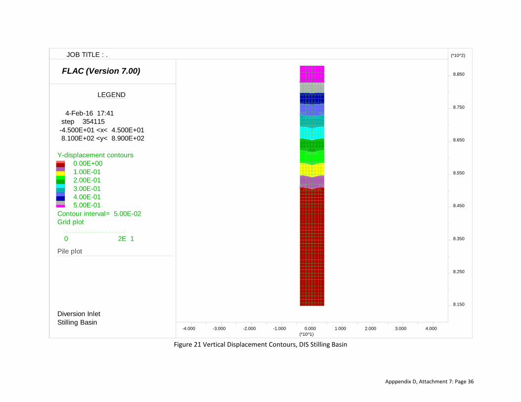
Figure 21 Vertical Displacement Contours, DIS Stilling Basin

FLAC (Version 7.00)

LEGEND

4-Feb-16 17:41 step 354115 -4.500E+01 <x< 4.500E+01 8.100E+02 <y< 8.900E+02

Y-displacement contours 0.00E+00 1.00E-01 2.00E-01 3.00E-01 4.00E-01 5.00E-01Contour interval= 5.00E-02Grid plot

0 2E 1

Pile plot

8.150

8.250

8.350

8.450

8.550

8.650

8.750

8.850

(*10^2)

-4.000 -3.000 -2.000 -1.000 0.000 1.000 2.000 3.000 4.000(*10^1)

JOB TITLE : .



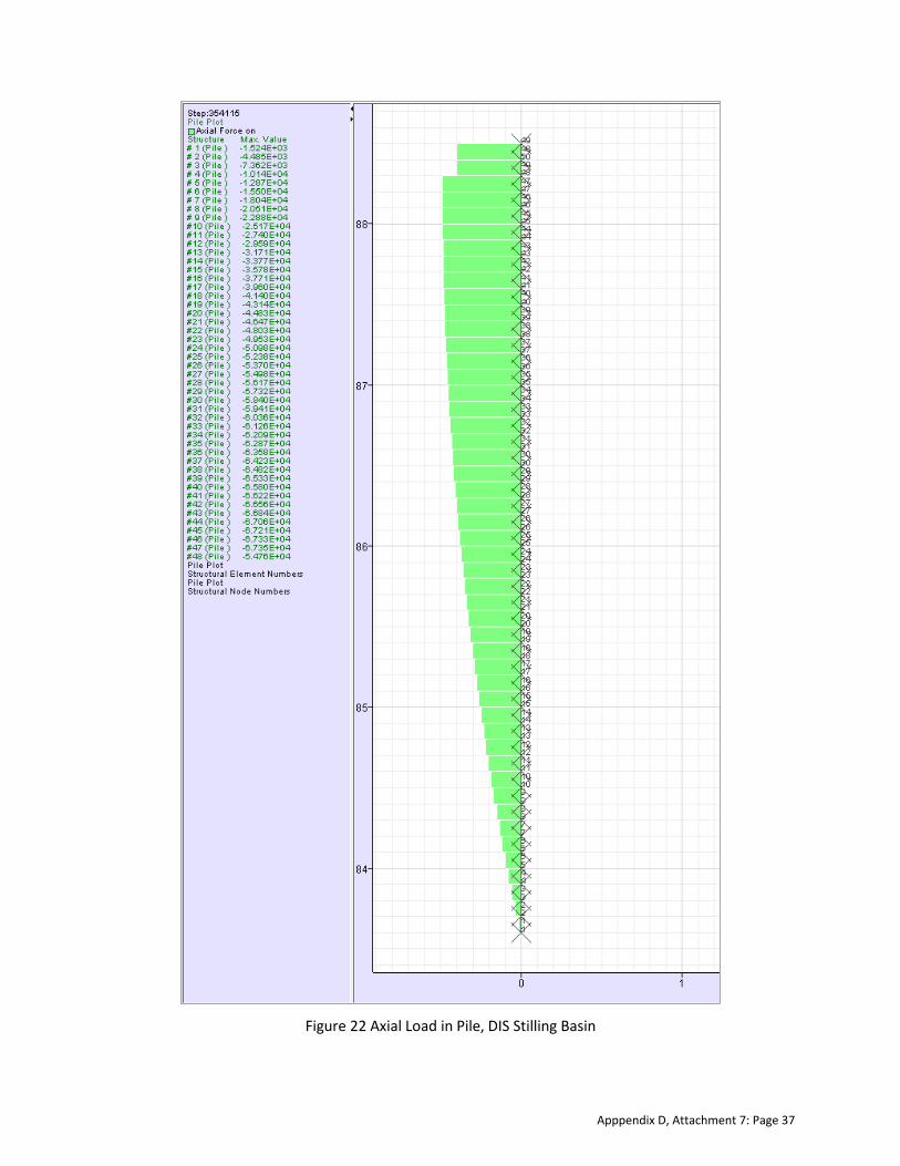
Figure 22 Axial Load in Pile, DIS Stilling Basin


Figure 23 Shear Spring Forces, DIS Stilling Basin


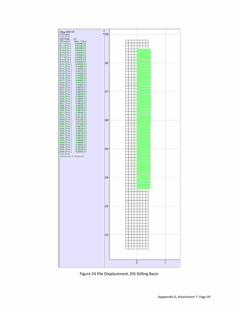
Figure 24 Pile Displacement, DIS Stilling Basin


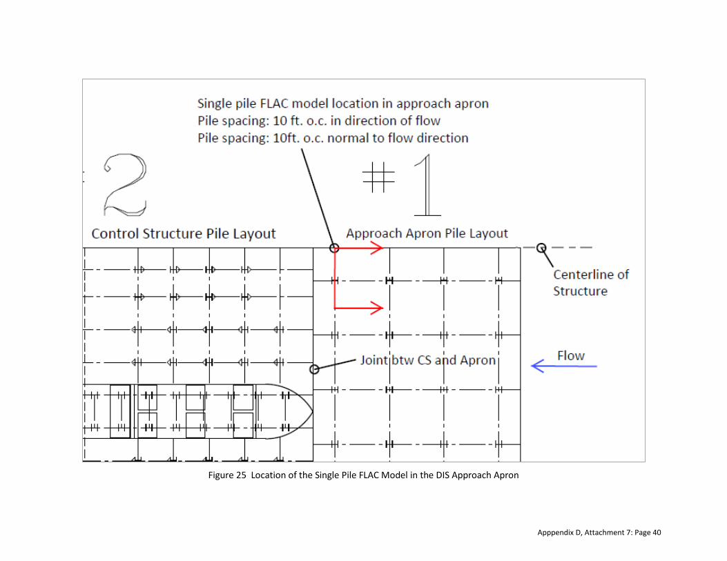
Figure 25 Location of the Single Pile FLAC Model in the DIS Approach Apron


Figure 26 FLAC model in DIS Approach Apron with Pile and Pile Cap (after unloading)

FLAC (Version 7.00)

LEGEND

4-Feb-16 16:49 step 129138 -4.500E+01 <x< 4.500E+01 8.100E+02 <y< 9.000E+02

User-defined Groups'User:Intact Till''User:Weathered Till'ArgusvilleBrennaSherackUser:Concrete

Grid plot

0 2E 1

Boundary plot

0 2E 1

Fixed Gridpoints

BXXXXXXXXXXXXXXXXXXXXXXXXXXXXXXXXXXXXXXXXXXXXXXXXXXXXXXXXXXXXXXXXXXXXXXXXXXXXXXXXXXXX

BBBBBBBBBBXXXXXXXXXXXXXXXXXXXXXXXXXXXXXXXXXXXXXXXXXXXXXXXXXXXXXXXXXXXXXXXXXXXXXXXXXXXXXXXXXXXX

X X-direction B Both directionsPile plot

8.150

8.250

8.350

8.450

8.550

8.650

8.750

8.850

8.950

(*10^2)

-4.000 -3.000 -2.000 -1.000 0.000 1.000 2.000 3.000 4.000(*10^1)

JOB TITLE : .

Diversion InletApproach Apron


Figure 27 Effective Vertical Stress Contours, 250 psf Contour Interval, DIS Approach Apron

FLAC (Version 7.00)

LEGEND

7-Feb-16 11:41 step 155309 -4.500E+01 <x< 4.500E+01 8.100E+02 <y< 9.000E+02

Effec. SYY-Stress Contours -4.50E+03 -3.75E+03 -3.00E+03 -2.25E+03 -1.50E+03 -7.50E+02 0.00E+00 7.50E+02 1.50E+03 2.25E+03


8.150

8.250

8.350

8.450

8.550

8.650

8.750

8.850

8.950

(*10 2̂)

-4.000 -3.000 -2.000 -1.000 0.000 1.000 2.000 3.000 4.000(*10 1̂)

JOB TITLE : .



Figure 28 Effective Horizontal Stress Contours, 250 psf Contour Interval, DIS Approach Apron

FLAC (Version 7.00)

LEGEND

7-Feb-16 11:43 step 155309 -4.500E+01 <x< 4.500E+01 8.100E+02 <y< 9.000E+02

Effec. SXX-Stress Contours -5.50E+03 -4.75E+03 -4.00E+03 -3.25E+03 -2.50E+03 -1.75E+03 -1.00E+03 -2.50E+02 5.00E+02


8.150

8.250

8.350

8.450

8.550

8.650

8.750

8.850

8.950

(*10 2̂)

-4.000 -3.000 -2.000 -1.000 0.000 1.000 2.000 3.000 4.000(*10 1̂)

JOB TITLE : .



Figure 29 Effective Vertical Stress Contours, 50 psf Contour Interval, DIS Approach Apron

FLAC (Version 7.00)

LEGEND

7-Feb-16 11:45 step 155309 -4.500E+01 <x< 4.500E+01 8.100E+02 <y< 9.000E+02

User-defined Groups'User:Intact Till''User:Weathered Till'ArgusvilleBrennaSherackUser:Concrete

Effec. SYY-Stress ContoursContour interval= 5.00E+01Minimum: -4.70E+03Maximum: 2.55E+03Pile plot

8.150

8.250

8.350

8.450

8.550

8.650

8.750

8.850

8.950

(*10 2̂)

-4.000 -3.000 -2.000 -1.000 0.000 1.000 2.000 3.000 4.000(*10 1̂)

JOB TITLE : .



Figure 30 Shear Strain Rate Contours, DIS Approach Apron

FLAC (Version 7.00)

LEGEND

7-Feb-16 13:49 step 155309 -4.500E+01 <x< 4.500E+01 8.100E+02 <y< 9.000E+02

Max. shear strain-rate 0.00E+00 2.50E-09 5.00E-09 7.50E-09 1.00E-08 1.25E-08 1.50E-08


0 2E 1

Pile plot

8.150

8.250

8.350

8.450

8.550

8.650

8.750

8.850

8.950

(*10 2̂)

-4.000 -3.000 -2.000 -1.000 0.000 1.000 2.000 3.000 4.000(*10 1̂)

JOB TITLE : .



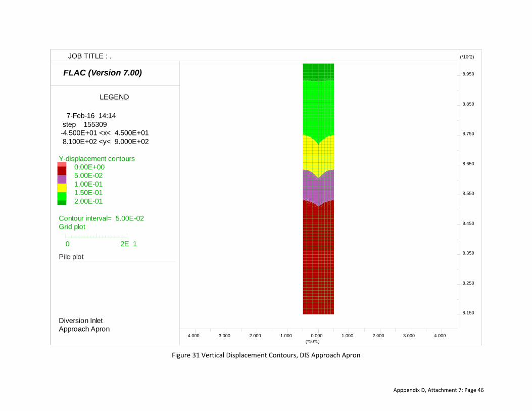
Figure 31 Vertical Displacement Contours, DIS Approach Apron

FLAC (Version 7.00)

LEGEND

7-Feb-16 14:14 step 155309 -4.500E+01 <x< 4.500E+01 8.100E+02 <y< 9.000E+02

Y-displacement contours 0.00E+00 5.00E-02 1.00E-01 1.50E-01 2.00E-01

Contour interval= 5.00E-02Grid plot

0 2E 1

Pile plot

8.150

8.250

8.350

8.450

8.550

8.650

8.750

8.850

8.950

(*10 2̂)

-4.000 -3.000 -2.000 -1.000 0.000 1.000 2.000 3.000 4.000(*10 1̂)

JOB TITLE : .



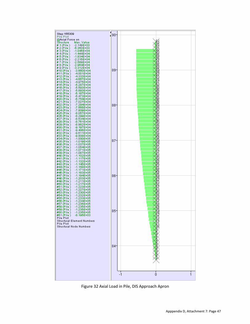
Figure 32 Axial Load in Pile, DIS Approach Apron


Figure 33 Shear Spring Force, DIS Approach Apron


Figure 34 Pile Displacement, DIS Approach Apron


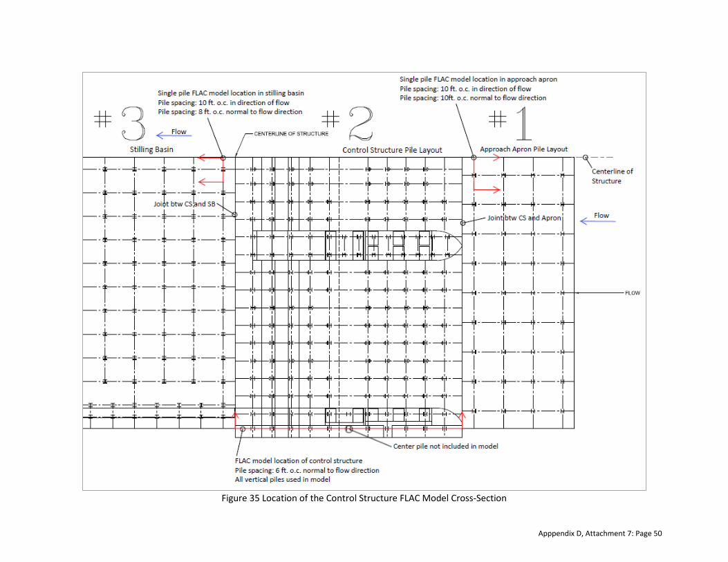
Figure 35 Location of the Control Structure FLAC Model Cross-Section


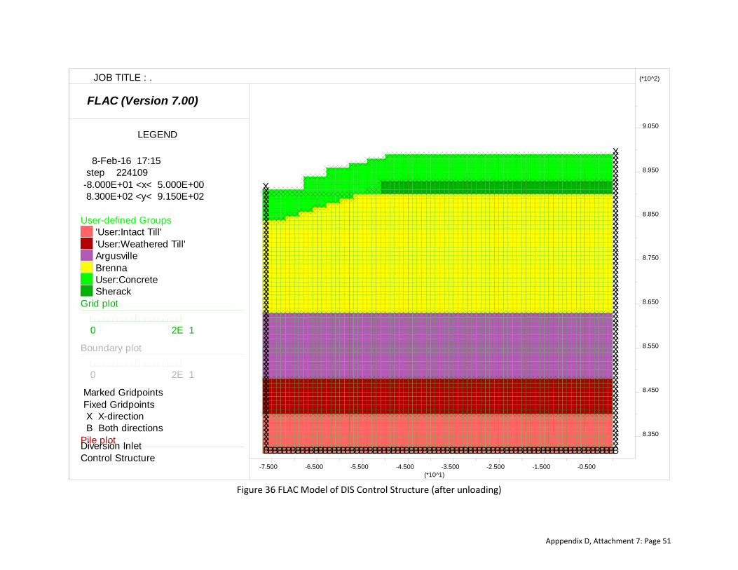
Figure 36 FLAC Model of DIS Control Structure (after unloading)

FLAC (Version 7.00)

LEGEND

8-Feb-16 17:15 step 224109 -8.000E+01 <x< 5.000E+00 8.300E+02 <y< 9.150E+02

User-defined Groups'User:Intact Till''User:Weathered Till'ArgusvilleBrennaUser:ConcreteSherack

Grid plot

0 2E 1

Boundary plot

0 2E 1

Marked Gridpoints Fixed Gridpoints

BXXXXXXXXXXXXXXXXXXXXXXXXXXXXXXXXXXXXXXXXXXXXXXXXXXXXXXXXXXXX

BBBBBBBBBBBBBBBBBBBBBBBBBBBBBBBBBBBBBBBBBBBBBBBBBBBBBBBBBBBBBBBBBBBBBBBBBBBBBXXXXXXXXXXXXXXXXXXXXXXXXXXXXXXXXXXXXXXXXXXXXXXXXXXXXXXXXXXXXXXXXXXXX

X X-direction B Both directionsPile plot

8.350

8.450

8.550

8.650

8.750

8.850

8.950

9.050

(*10^2)

-7.500 -6.500 -5.500 -4.500 -3.500 -2.500 -1.500 -0.500(*10^1)

JOB TITLE : .

Diversion InletControl Structure


Figure 37 Effective Vertical Stress Contours, DIS Control Structure (after unloading)

FLAC (Version 7.00)

LEGEND

10-Feb-16 9:49 step 224109 -8.000E+01 <x< 5.000E+00 8.300E+02 <y< 9.150E+02

Boundary plot

0 2E 1

Effec. SYY-Stress Contours -4.00E+03 -3.00E+03 -2.00E+03 -1.00E+03 0.00E+00 1.00E+03 2.00E+03

Contour interval= 1.00E+03Extrap. by averagingPile plot Marked GridpointsWater Table

8.350

8.450

8.550

8.650

8.750

8.850

8.950

9.050

(*10^2)

-7.500 -6.500 -5.500 -4.500 -3.500 -2.500 -1.500 -0.500(*10^1)

JOB TITLE : .



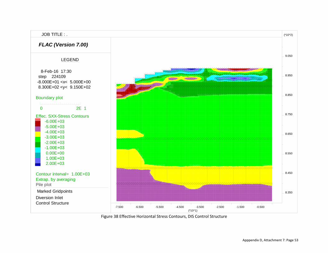
Figure 38 Effective Horizontal Stress Contours, DIS Control Structure

FLAC (Version 7.00)

LEGEND

8-Feb-16 17:30 step 224109 -8.000E+01 <x< 5.000E+00 8.300E+02 <y< 9.150E+02

Boundary plot

0 2E 1

Effec. SXX-Stress Contours -6.00E+03 -5.00E+03 -4.00E+03 -3.00E+03 -2.00E+03 -1.00E+03 0.00E+00 1.00E+03 2.00E+03

Contour interval= 1.00E+03Extrap. by averagingPile plot Marked Gridpoints 8.350

8.450

8.550

8.650

8.750

8.850

8.950

9.050

(*10^2)

-7.500 -6.500 -5.500 -4.500 -3.500 -2.500 -1.500 -0.500(*10^1)

JOB TITLE : .



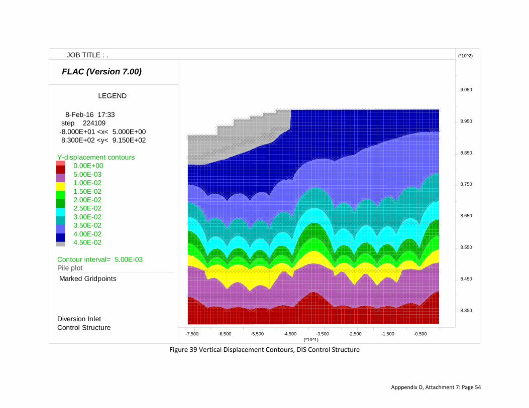
Figure 39 Vertical Displacement Contours, DIS Control Structure

FLAC (Version 7.00)

LEGEND

8-Feb-16 17:33 step 224109 -8.000E+01 <x< 5.000E+00 8.300E+02 <y< 9.150E+02

Y-displacement contours 0.00E+00 5.00E-03 1.00E-02 1.50E-02 2.00E-02 2.50E-02 3.00E-02 3.50E-02 4.00E-02 4.50E-02

Contour interval= 5.00E-03Pile plot Marked Gridpoints

8.350

8.450

8.550

8.650

8.750

8.850

8.950

9.050

(*10^2)

-7.500 -6.500 -5.500 -4.500 -3.500 -2.500 -1.500 -0.500(*10^1)

JOB TITLE : .



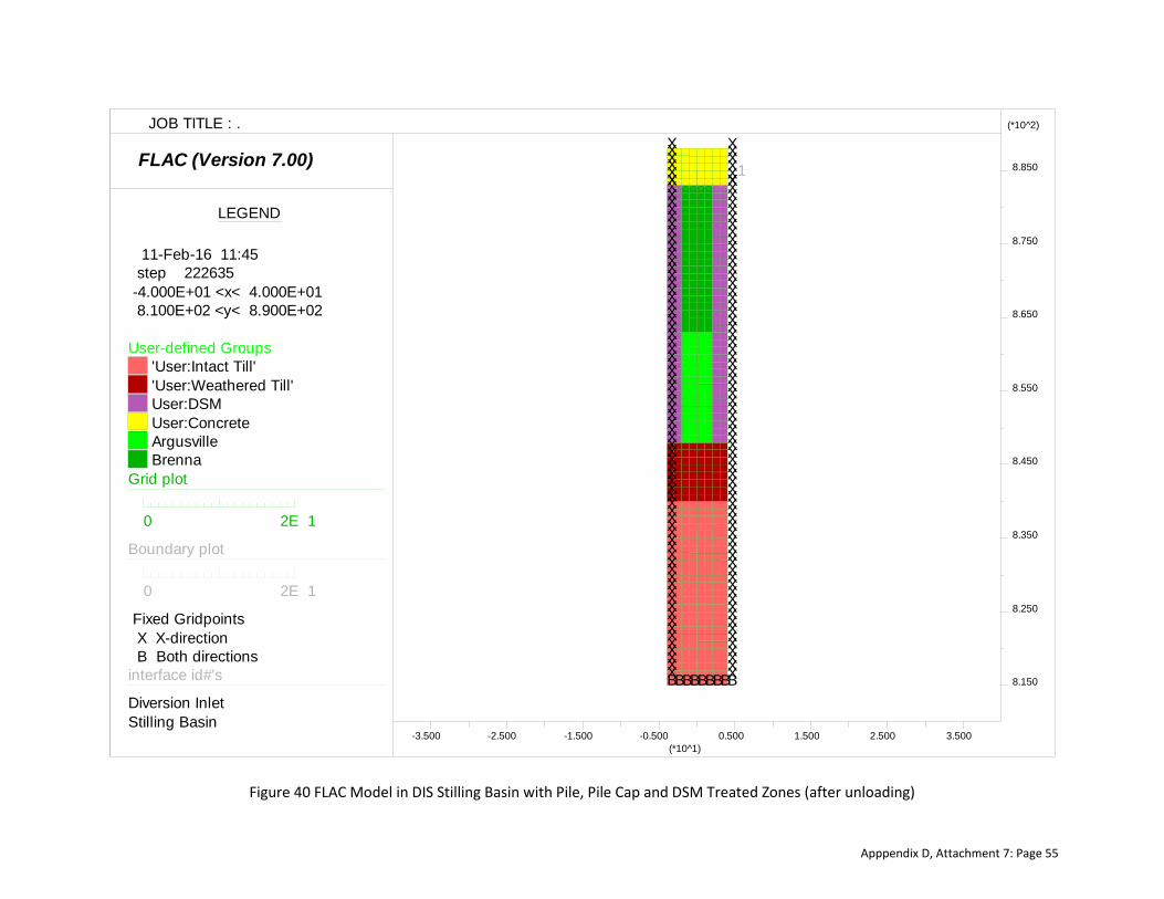
Figure 40 FLAC Model in DIS Stilling Basin with Pile, Pile Cap and DSM Treated Zones (after unloading)

FLAC (Version 7.00)

LEGEND

11-Feb-16 11:45 step 222635 -4.000E+01 <x< 4.000E+01 8.100E+02 <y< 8.900E+02

User-defined Groups'User:Intact Till''User:Weathered Till'User:DSMUser:ConcreteArgusvilleBrenna

Grid plot

0 2E 1

Boundary plot

0 2E 1

Fixed Gridpoints

BXXXXXXXXXXXXXXXXXXXXXXXXXXXXXXXXXXXXXXXXXXXXXXXXXXXXXXXXXXXXXXXXXXXXXXXXXX

BBBBBBBBXXXXXXXXXXXXXXXXXXXXXXXXXXXXXXXXXXXXXXXXXXXXXXXXXXXXXXXXXXXXXXXXXXXXXXXXXX

X X-direction B Both directionsinterface id#'s

1

8.150

8.250

8.350

8.450

8.550

8.650

8.750

8.850

(*10^2)

-3.500 -2.500 -1.500 -0.500 0.500 1.500 2.500 3.500(*10^1)

JOB TITLE : .



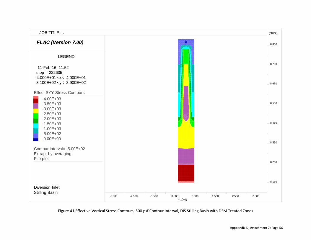
Figure 41 Effective Vertical Stress Contours, 500 psf Contour Interval, DIS Stilling Basin with DSM Treated Zones

FLAC (Version 7.00)

LEGEND

11-Feb-16 11:52 step 222635 -4.000E+01 <x< 4.000E+01 8.100E+02 <y< 8.900E+02

Effec. SYY-Stress Contours -4.00E+03 -3.50E+03 -3.00E+03 -2.50E+03 -2.00E+03 -1.50E+03 -1.00E+03 -5.00E+02 0.00E+00


8.150

8.250

8.350

8.450

8.550

8.650

8.750

8.850

(*10^2)

-3.500 -2.500 -1.500 -0.500 0.500 1.500 2.500 3.500(*10^1)

JOB TITLE : .



Figure 42 Effective Horizontal Stress Contours, 500 psf Contour Interval, DIS Stilling Basin with DSM Treated Zones

FLAC (Version 7.00)

LEGEND

11-Feb-16 12:23 step 222635 -4.000E+01 <x< 4.000E+01 8.100E+02 <y< 8.900E+02

Effec. SXX-Stress Contours -5.00E+03 -4.50E+03 -4.00E+03 -3.50E+03 -3.00E+03 -2.50E+03 -2.00E+03 -1.50E+03 -1.00E+03


8.150

8.250

8.350

8.450

8.550

8.650

8.750

8.850

(*10^2)

-3.500 -2.500 -1.500 -0.500 0.500 1.500 2.500 3.500(*10^1)

JOB TITLE : .



Figure 43 Effective Vertical Stress Contours, 50 psf Contour Interval, DIS Stilling Basin with DSM Treated Zones

FLAC (Version 7.00)

LEGEND

11-Feb-16 12:28 step 222635 -1.500E+01 <x< 1.500E+01 8.300E+02 <y< 8.600E+02

User-defined Groups'User:Intact Till''User:Weathered Till'User:DSMArgusville

Effec. SYY-Stress ContoursContour interval= 1.00E+02Minimum: -3.50E+03Maximum: -9.00E+02Pile plot

8.325

8.375

8.425

8.475

8.525

8.575

(*10^2)

-1.250 -0.750 -0.250 0.250 0.750 1.250(*10^1)

JOB TITLE : .



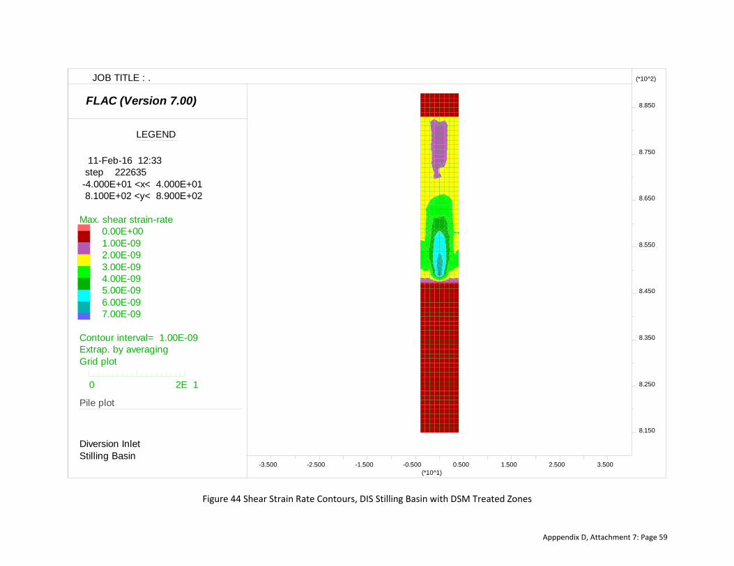
Figure 44 Shear Strain Rate Contours, DIS Stilling Basin with DSM Treated Zones

FLAC (Version 7.00)

LEGEND

11-Feb-16 12:33 step 222635 -4.000E+01 <x< 4.000E+01 8.100E+02 <y< 8.900E+02

Max. shear strain-rate 0.00E+00 1.00E-09 2.00E-09 3.00E-09 4.00E-09 5.00E-09 6.00E-09 7.00E-09


0 2E 1

Pile plot

8.150

8.250

8.350

8.450

8.550

8.650

8.750

8.850

(*10^2)

-3.500 -2.500 -1.500 -0.500 0.500 1.500 2.500 3.500(*10^1)

JOB TITLE : .



Figure 45 Shear Stress Contours, 25 psf Contour Interval, DIS Stilling Basin with DSM Treated Zones

FLAC (Version 7.00)

LEGEND

12-Feb-16 11:18 step 222635 -4.000E+01 <x< 4.000E+01 8.100E+02 <y< 8.900E+02

XY-stress contours 0.00E+00 5.00E+01 1.00E+02 1.50E+02 2.00E+02 2.50E+02 3.00E+02 3.50E+02Contour interval= 2.50E+01Extrap. by averagingPile PlotPile Locations

8.150

8.250

8.350

8.450

8.550

8.650

8.750

8.850

(*10^2)

-3.500 -2.500 -1.500 -0.500 0.500 1.500 2.500 3.500(*10^1)

JOB TITLE : .



Figure 46 Shear Stress Contours, 50 psf Contour Interval, DIS Stilling Basin with DSM Treated Zones

FLAC (Version 7.00)

LEGEND

11-Feb-16 15:48 step 222635 -1.500E+01 <x< 1.500E+01 8.300E+02 <y< 8.600E+02

User-defined Groups'User:Intact Till''User:Weathered Till'User:DSMArgusville

XY-stress contoursContour interval= 5.00E+01Minimum: 0.00E+00Maximum: 3.50E+02Pile plot

8.325

8.375

8.425

8.475

8.525

8.575

(*10^2)

-1.250 -0.750 -0.250 0.250 0.750 1.250(*10^1)

JOB TITLE : .



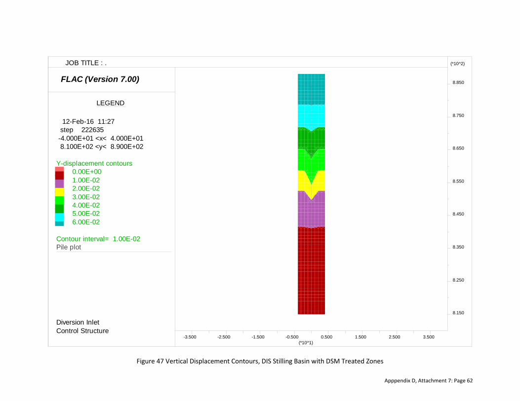
Figure 47 Vertical Displacement Contours, DIS Stilling Basin with DSM Treated Zones

FLAC (Version 7.00)

LEGEND

12-Feb-16 11:27 step 222635 -4.000E+01 <x< 4.000E+01 8.100E+02 <y< 8.900E+02

Y-displacement contours 0.00E+00 1.00E-02 2.00E-02 3.00E-02 4.00E-02 5.00E-02 6.00E-02

Contour interval= 1.00E-02Pile plot

8.150

8.250

8.350

8.450

8.550

8.650

8.750

8.850

(*10^2)

-3.500 -2.500 -1.500 -0.500 0.500 1.500 2.500 3.500(*10^1)

JOB TITLE : .



Figure 48 Axial Load in Pile, DIS Stilling Basin with DSM Treated Zones


Figure 49 Pile Displacement, DIS Stilling Basin with DSM Treated Zones


Figure 50 Proposed DSM Panel Layout for DIS Stilling Basin


attachment d-7: rebound and uplift of the stilling basin ... · figure 40 flac model in dis...

Documents