attachment b-2 - marylanddnr.maryland.gov/waters/bay/documents/lsrwa/reports/appb2.pdf · erosion...
TRANSCRIPT

B-2
1
Attachment B-2
Sedflume Erosion Data and Analysis
The Conowingo Reservoir sediment bed is composed of cohesive sediments. Non-cohesive sediment
(sand and gravel) erosion and settling can be generally estimated from grain size distribution and mineral density. Cohesive sediment transport processes are dominated by other factors. Cohesive sediments are generally a mixture of sand, silt, and clay sized particles.
A general definition for cohesive sediment is sediment for which the erosion rate cannot be estimated by standard sand/gravel transport methods. In these cases, cohesive forces are equivalent to or are greater than the gravitational forces that dominate sand transport. Cohesive sediment erosion characteristics are highly dependent upon factors such as particle size distribution, particle coatings, fine sediment mineralo- gy, organic content, bulk density, gas content, pore-water chemistry, and biological activity. Erosion rate and critical shear stress for erosion can vary significantly with small changes in only one of these inter- dependent parameters. It has been well demonstrated that critical stress and erosion rates for cohesive sed- iment can vary over several orders of magnitude for sediments with only slightly differing properties. Therefore, the influence of cohesion on sediment processes is significant. Qualitatively, it is understood which properties most significantly influence erosion. However, there are no quantitative methods availa- ble to determine erosion rate from cohesive sediment properties. Therefore, due to the sensitivity and wide range of influencing parameters, erosion characteristics of cohesive sediments are determined by site-specific analysis of erosion with erosion flumes.
Several flumes are available to parameterize site-specific cohesive sediment erosion algorithms. Most of these devices operate over a range of low shear stress (<2 Pa) and are consequently capable of measur- ing only surface sediment erosion. Sedflume is an erosion device with capability to impose bed stresses in the range of 0.1 to 12 Pa and measures erosion rates from sediment cores taken from the field (for in-situ or stratified bed conditions) or prepared in the laboratory (for assessing disturbed sediments such as dredged material). Sedflume is designed to quantify erosion rates for surface and sub-surface sediments. These measurements permit description of the vertical variation of erosion rate within the bed. It should be noted that even if sediments are well mixed, cohesive sediment bed erosion will change with depth due to the influence of consolidation (bed density) on erosion rate. Erosion rate can vary by several orders of magnitude between surficial sediments and sediment buried less than 30 cm below the surface. Sedflume was selected to quantify erosion rate and erosion rate variation with depth (density) for this study.
Methods
This section describes the field experiments, sampling and experimental methods, and data analysis methods used in determining cohesive sediment erosion within Conowingo Reservoir. Background and technical information about the experimental device is presented first, followed by description of how these devices were deployed during field experiments to meet the study objectives.

B-2
2
Figure 1. Sedflume erosion flume (lower right). Core inserted into test section (upper left). Core surface flush with bottom of flow channel (upper right). Table of shear stress associated with channel flow rates (lower left).
Sedflume
Sedflume is a field- or laboratory-deployable flume for quantifying cohesive sediment erosion. The
USACE-developed Sedflume is a derivative of the flume developed by researchers at the University of California at Santa Barbara (McNeil et al. 1996). The flume includes an 80-cm-long inlet section (Figure 1) with cross-sectional area of 2 × 10 cm for uniform, fully developed, smooth-turbulent flow. The inlet section is followed by a 15-cm-long test section with a 10 × 15 cm open bottom (the open bottom can ac- cept cores with rectangular cross-section (10 × 15 cm) or circular cross-section (10-cm diameter) ). Cor- ing tubes and flume test section, inlet section, and exit sections are constructed of clear polycarbonate materials to permit observation of sediment-water interactions during the course of erosion experiments. The flume includes a port over the test section to provide access to the core surface for physical sampling. The flume accepts sediment cores up to 80-cm in length.
Erosion Experiments
Prior to the erosion experiment, descriptions of the core are recorded, including length, condition of
the core surface, biological activity, and any visual evidence of layering. Cores are inserted into the test- ing section of Sedflume and a screw jack is used to advance the plunger such that the core surface be- comes flush with the bottom wall of the flume. Flow is directed over the sample by diverting flow from a

B-2
3
3-hp pump, through a 5-cm inner diameter hose, into the flume. The flow through the flume produces shear stress on the surface of the core. (Numerical, experimental, and analytical analyses have been per- formed to relate flowrate to bottom shear stress.) Erosion of the surface sediment is initiated as the shear stress is increased beyond the critical stress for erosion, τcr. As sediment erodes from the core surface, the operator advances the screw jack to maintain the sediment surface flush with the bottom wall of the ero- sion flume. Figure 1 includes a photograph of the flume, a close-up photograph of the test section, and a table of flow rate/shear stress relationships.
Erosion rate is determined from the displacement of the core surface over the elapsed time of the ex- periment. Generally, erosion experiments are performed in repeating sequences of increasing shear stress. Operator experience permits sequencing of erosion tests to allow greater vertical resolution of shear stress/erosion rate data where required. The duration of each erosion experiment at a specified shear stress is dependent on the rate of erosion and generally is between 0.25 and 15 minutes. Shear stresses that in- duce no measurable erosion are also recorded. The range of shear stress for each cycle is determined by the operator based on the previous erosion sequences and erosion behavior during the ongoing sequence.
Sediment Bulk Properties
Physical samples for bulk sediment property measurements are taken at approximately 3-5 cm inter-
vals during erosion experiments, generally at the end of each shear stress cycle. Physical samples are collected by draining the flume channel, opening the port over the test section, and extracting a sample from the sediment bed. Properties measured include bulk density and grain-size distribution, and separate samples were collected from the core surface for these analyses. These properties strongly influence ero- sion; therefore, understanding their variation with depth is important in interpreting the erosion data.
Bulk Density Measurements. Bulk sediment density of physical samples is determined by a wet-dry weight analysis. Physical samples are extracted from the saturated core surface and placed in a pre- weighed aluminum tray. Sample weight is recorded immediately after collection and again after a mini- mum of 12 hours in an 90° C (194° F) drying oven. Wet weight of the sample was calculated by subtract- ing tare weight from the weight of the sample. The dry weight of the sample was calculated as the tare weight subtracted from the weight after drying. The water content w is then given
m � m w
w d (1)
md
where mw and md are the wet and dry weights, respectively. A volume of saturated sed- iment, V, consists of both solid particles and water and can be written as
V Vs Vw (2)
where Vs is the volume of solid particles and Vw is the volume of water. If the sediment particles and water have density �s and �w, respectively, the water content of the sedi-
ment can be written as
w wVw
sVs
(3)
A mass balance of the volume of sediment gives

B-2
4
V sVs wVw (4)
where is the bulk density of the sediment sample.
(1)-(4) are used to derive an explicit expression for the bulk density of the sediment sample, , as a function of the water content, w, and the densities of the sediment particles and water. This equation is
s w �
s w s
w ws
(5)
For the purpose of these calculations, s = 2.65 g·cm-3 and w is calculated for measured pore water at sample temperature.
Particle-Size Distribution. Samples collected during erosion experiments were transported to the Sed- iment Transport Processes Lab at ERDC for grain size analysis. A Beckman-Coulter LS 13-320 laser particle-sizer was used to measure the particle-size distributions in sub-samples collected from the cores. The LS 13-320 measures particle size over the range 0.4 to 900 μm. Particle size distributions were measured by first removing and sieving particles larger than 850 μm. The passing portion of the sample was added to a small volume of water (approximately 150 mL) and sonicated using a high-powered la- boratory sonicator to disperse the sediment. The dispersed solution was placed in the particle sizer fluid module. The sample is pumped and recirculated through the optical module. The optical module in- cludes a spatial filter assembly containing a laser diode and laser beam collimator. The diffraction detec- tor assembly contains a custom photodetector array that is used for the measurement of light scattering by the suspended particles. The distribution of grain sizes and median grain sizes is derived from this light scattering measurement. The size distribution of fines passing the 850 μm sieve is scaled to account for the sediment mass retained on the sieve. Organic material was not oxidized before grain size analysis was performed; therefore grain size distributions include organic material.
Multivariate Erosion Rate Prediction
The goal of erosion data analysis is to determine appropriate parameterization of erosion processes for numerical modeling studies. For this study, the erosion data are to be described in the SEDZLJ mod- el. SEDZLJ is flexible in the form of the erosion equation, and the effects of bulk density, depth, and ap- plied shear stress may be represented as indicated by the erosion data. Analysis of the erosion data from Conowingo Reservoir suggested that the erosion algorithm should be of the following form:
E 0;
E A n ;
c
c m
(6)
E A n ; m m
where E represents erosion rate (cm⋅s-1) from the bed, τ is bed shear stress, τc is critical stress for erosion, A is an empirical constant, n is an empirical exponent, and τm is bed stress at which erosion rate becomes constant. Solution of Equation (6) to data requires solving for three parameters, τc, A, and n. Bed stress for the upper limit of erosion rate is determined by examining the data. The best fit of Equation (6) to measured data is accomplished through an iterative, multi-parameter, least-squares method on the linear transform of Equation (6).
B-2
5
Field Experiments
Field experiments were conducted from April 11 through April 16 of 2012. Field experiments in- cluded core collection, physical sampling, and cohesive sediment erosion experiments.
Core Collection
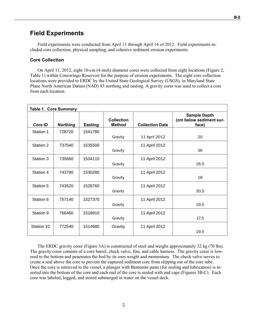
On April 11, 2012, eight 10-cm (4-inch) diameter cores were collected from eight locations (Figure 2,
Table 1) within Conowingo Reservoir for the purpose of erosion experiments. The eight core collection locations were provided to ERDC by the United State Geological Survey (USGS), in Maryland State Plane North American Datum (NAD) 83 northing and easting. A gravity corer was used to collect a core from each location.
Table 1. Core Summary
Core ID
Northing
Easting Collection
Method
Collection Date
Sample Depth (cm below sediment sur-
face)
Station 1 728720 1541780 Gravity
11 April 2012
20
Station 2 737040 1535500 Gravity
11 April 2012 36
Station 3 735660 1534110 Gravity
11 April 2012 26.5
Station 4 743790 1530280 Gravity
11 April 2012 18
Station 5 743520 1528760 Gravity
11 April 2012 30.5
Station 6 757140 1527370 Gravity
11 April 2012 19.5
Station 9 766460 1518910 Gravity
11 April 2012 17.5
Station 10 772540 1514680 Gravity 11 April 2012 19.5
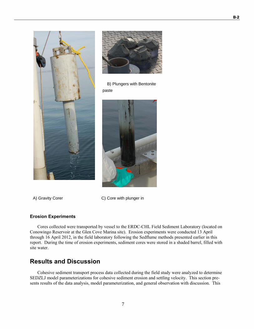
The ERDC gravity corer (Figure 3A) is constructed of steel and weighs approximately 32 kg (70 lbs). The gravity corer consists of a core barrel, check valve, fins, and cable harness. The gravity corer is low- ered to the bottom and penetrates the bed by its own weight and momentum. The check valve serves to create a seal above the core to prevent the captured sediment core from slipping out of the core tube. Once the core is retrieved to the vessel, a plunger with Bentonite paste (for sealing and lubrication) is in- serted into the bottom of the core and each end of the core is sealed with end caps (Figures 3B-C). Each core was labeled, logged, and stored submerged in water on the vessel deck.

B-2
6
Figure 2. Coring locations in Conowingo Reservoir, MD.
B-2
7
B) Plungers with Bentonite
paste
A) Gravity Corer C) Core with plunger in
Erosion Experiments
Cores collected were transported by vessel to the ERDC-CHL Field Sediment Laboratory (located on
Conowingo Reservoir at the Glen Cove Marina site). Erosion experiments were conducted 13 April through 16 April 2012, in the field laboratory following the Sedflume methods presented earlier in this report. During the time of erosion experiments, sediment cores were stored in a shaded barrel, filled with site water.
Results and Discussion
Cohesive sediment transport process data collected during the field study were analyzed to determine SEDZLJ model parameterizations for cohesive sediment erosion and settling velocity. This section pre- sents results of the data analysis, model parameterization, and general observation with discussion. This

B-2
8
report presents physical descriptions of each core including:, bed density profiles, grain size analysis, and erosion analysis of each core, including definition of bed layers that erode similarly.
Cohesive Sediment Erosion
Analysis of cohesive sediment erosion data obtained from undisturbed field cores is inherently com-
plex. Cohesive sediment erosion is sensitive to slight changes in bed density, deposit mineralogy, gas content, organic content, biological activity, debris and a host of other factors. In many cases, these fac- tors change significantly at relatively small vertical scales (such as depositional bed sequences). Conse- quently, measured cohesive sediment erosion rates from field cores are notoriously variable. To compensate for the large variance in measured erosion rates, field erosion experiments are conducted in a manner to produce a large sample from which to derive statistically representative relationships for vari- ous numerical erosion algorithms. To ensure high quality in the data analysis, data and associated exper- imental notes are evaluated to identify outliers in the dataset. Outliers are rejected based on comparisons between adjacent data points and experimental log notes.
Cores 1-5 (from the downstream half of the reservoir) were composed primarily of silt and clay and the sediment composition was fairly uniform with depth aside from the occasional increase in leafy or- ganic matter or the occasional sand lens. Sand content generally increased upstream of Core 6 and sedi- ment composition became more variable with depth. The composition of Core 10 was highly variable with depth, with as much as 80% sand content.
Erosion Parameterization
Erosion rate data were evaluated for relationships between erosion rate, bed density, and applied
shear stress. In general, the erosion behavior of the cores gradually varied with depth. The occasional sand lens or change in organic content occasionally produced distinctly different erosion behavior. The erosion data were grouped in layers to account for the changing critical erosion depth and erosion rates with depth.
The erosion data from Core 1 will be presented here to illustrate the parameterization of the erosion data from Conowingo Reservoir. The composition of Core 1 was very uniform and was predominantly silt (80-85% silt from the physical samples). Figure 3 presents the erosion data with depth. First, the ero- sion data were grouped vertically within cores. This grouping was accomplished by reviewing the ero- sion notes and erosion rate relationships to depth, density, and shear stress. At the sediment water interface, there is typically a thin, low-density layer that erodes more easily than the more highly consoli- dated sediments deeper in the sediment bed. This was observed for Core 1 between depths of 0 – 4 cm into the core with a critical shear stress of 0.2 Pa, which is defined as Layer Core01_L1. Beneath the sur- face layer was a layer from 5 – 10 cm that had a critical shear stress of 0.4 Pa, and reduced erosion rate associated with the increase in bed density with depth into the core. Core01_L3 (10-14 cm depth) was associated with an increase in critical shear stress to 0.8 Pa and further reduction of erosion rates with depth into the core.

B-2
9
Figure 3. Erosion rate data of Core 1. For erosion rate data set, colors indicate the layers of the core as inferred from erosion data visual observations and physical properties
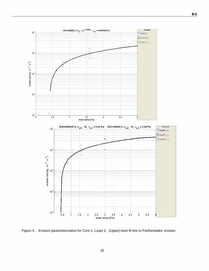
A multivariate, least-squares fit of erosion rate to shear stress for the standard form of the
Partheniades erosion equation (Core 01, Layer 2) is presented in the upper plot of Figure 4. In the bottom plot of Figure 4, a parameterization of the piece-wise linear form of the Partheniades implementation in HEC-RAS is presented. Erosion parameterization for each layer in each core is provided in Table 2 (Full Partheniades) and Table 3 (HEC-RAS Partheniades). For instances where the range of erosion measurements was nearly linear, the second limb of the HEC-RAS parameterization is not provided.
B-2
10
Figure 4. Erosion parameterization for Core 1, Layer 2. (Upper) best-fit line to Partheniades’ erosion

B-2
11
All cores collected exhibited cohesive erosion behavior. Critical shear stress for erosion generally in- creased with depth and erosion rates at a given shear stress decreased with depth. These are common ob- servations associated with stronger bonding with increased sediment consolidation and density.
Table 2. Cohesive Sediment Erosion Parameterization
Layer ID
Depth (cm)
Critical Shear (τcr)
Erosion Rate Con-
stant (M)
Erosion Rate Ex-
ponent (n)
Pa - -
Core01_L1 0-4 0.20 2.02E-02 1.14
Core01_L2 5-10 0.40 2.89E-02 1.10
Core01_L3 10-14 0.80 3.52E-02 0.96
Core02_L1 0-10 0.20 1.01E-01 1.05
Core02_L2 10-17 0.40 5.98E-02 1.52
Core02_L3 17-24 0.80 3.73E-02 1.36
Core02_L4 24-32 1.60 9.18E-02 0.92
Core02_L3&4 17-32 0.80 3.86E-02 0.92
Core03_L1 0-2.5 0.20 9.90E-03 0.98
Core03_L2 2.5-22 0.80 8.08E-02 1.00
Core04_L1 0-2 0.20 1.04E-02 1.21
Core04_L2 2-11 0.80 3.23E-02 0.90

B-2
12
Table 2. Cohesive Sediment Erosion Parameterization
Layer ID
Depth (cm)
Critical Shear (τcr)
Erosion Rate Con-
stant (M)
Erosion Rate Ex-
ponent (n)
Pa - -
Core05_L1 0-5 0.20 1.20E-02 1.04
Core05_L2 5-12 0.78 2.17E-02 1.37
Core05_L3 12-24 1.60 9.80E-02 0.99
Core06_L1 0-2 0.10 1.48E-02 0.90
Core06_L2 2-14 1.60 3.31E-02 1.04
Core09_L1 0-2 0.20 8.20E-03 1.41
Core09_L2 2-9 1.52 2.32E-02 1.36
Core10_L1 0-8 0.18 3.40E-02 1.31
Core10_L2 8-16 1.14 1.70E-02 1.61

B-2
13
Table 3. Cohesive Sediment Erosion Parameterization for HEC-RAS
Layer ID
Depth
(cm)
Shear Thresh-
old
Erosion Rate
Mass Wasting
Threshold
Mass Wasting Rate
Pa lb/ft2 kg/m2/s lb/ft2/hr Pa lb/ft2 kg/m2/s lb/ft2/hr
Core01_L1 0-4 0.2 0.0042 2.02E-02 14.9 1 0.0209 0.263 193.9099
Core01_L2 5-10 0.4 0.0084 3.24E-02 23.9 - - - -
Core01_L3 10-14 0.8 0.0167 3.39E-02 25.0 - - - -
Core02_L1 0-10 0.2 0.0042 1.04E-01 76.7 - - - -
Core02_L2 10-17 0.4 0.0084 6.32E-02 46.6 0.9 0.0188 0.323 238
Core02_L3 17-24 0.8 0.0167 4.62E-02 34.1 - - - -
Core02_L4 24-32 1.6 0.0334 8.86E-02 65.3 - - - -
Core02_L3&4 17-32 0.8 0.0167 3.53E-02 26.0 - - - -
Core03_L1 0-2.5 0.2 0.0042 9.60E-03 7.08 - - - -
Core03_L2 2.5-22 0.8 0.0167 8.07E-02 59.5 - - - -
Core03_L1&2 0-22 0.2 0.0042 1.09E-02 8.04 2 0.0418 0.237 175
Core04_L1 0-2 0.2 0.0042 1.20E-02 8.85 0.8 0.0167 0.087 64.1
Core04_L2 2-11 0.8 0.0167 2.82E-02 20.8 - - - -
Core05_L1 0-5 0.2 0.0042 1.28E-02 9.44 - - - -
Core05_L2 5-12 0.8 0.0167 2.22E-02 16.4 2 0.0418 0.125 92.2

B-2
14
Table 3. Cohesive Sediment Erosion Parameterization for HEC-RAS
Layer ID
Depth
(cm)
Shear Thresh-
old
Erosion Rate
Mass Wasting
Threshold
Mass Wasting Rate
Pa lb/ft2 kg/m2/s lb/ft2/hr Pa lb/ft2 kg/m2/s lb/ft2/hr
Core05_L3 12-24 1.6 0.0334 9.76E-02 72.0 - - - -
Core06_L1 0-2 0.1 0.0021 1.32E-02 9.73 - - - -
Core06_L2 2-14 1.59 0.0332 3.41E-02 25.1 - - - -
Core09_L1 0-2 0.2 0.0042 1.25E-02 9.22 0.8 0.0167 0.102 75.2
Core09_L2 2-9 1.58 0.033 3.43E-02 25.3 - - - -
Core10_L1 0-8 0.19 0.004 5.08E-02 37.5 - - - -
Core10_L2 8-16 1.19 0.0249 1.95E-02 14.4 2.8 0.0585 0.139 102
Summary
United States Army Corp of Engineers, Baltimore District commissioned the ERDC to conduct cohe- sive sediment erosion testing services for the purpose of defining erosion rates of reservoir bottom sedi- ments at Conowingo Reservoir, Maryland. ERDC-CHL conducted the erosion testing in April 2012.
Eight, 4-inch (10-cm) diameter sediment cores were collected from the locations throughout Conowingo Reservoir. The cores were eroded in the Field Sediment Transport Laboratory that was oper- ated at the Glen Cove Marina. During erosion experiments, the cores were visually described, eroded, and subsampled for physical properties. Erosion data were analyzed by the layers evident in each core and later grouped by core layers that demonstrated similar erosion characteristics. Empirical coefficients were determined for modeling cohesive sediment bed erosion for individual core layers and groups of core layers that had similar erosion behavior.
Acknowledgements
Mr. Michael Langland from the United States Geological Survey (USGS) provided background in- formation on Conowingo Reservoir and recommended sediment sampling locations for the field data col- lection and analysis. Mr. Mike and Tommy Kirklin (contractors for USACE-CHL) assisted with core collection, erosion experiments, and sample analysis.

B-2
15
References
Jepsen, R., Roberts, J, and Lick, W. 1997a. ‘Effects of bulk density on sediment erosion rates’, Water,
Air, and Soil Pollution, 99, 21-31.

B-2
16
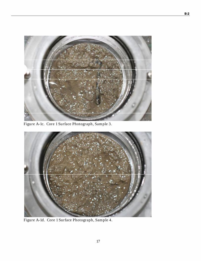
Core Physical Properties
Figure A-1a. Core 1 Surface Photograph, Sample 1.
Figure A-1b. Core 1 Surface Photograph, Sample 2.
B-2
17
Figure A-1c. Core 1 Surface Photograph, Sample 3.
Figure A-1d. Core 1 Surface Photograph, Sample 4.

B-2
18
Figure A-1e. Core 1 Surface Photograph, Sample 5.
Table A-1b. Physical Sample Properties (Core 1)
Sample
Depth
(cm below
surf)
Bulk den-
sity
(g/cm3)
D10(µm)
D50(µm)
D90(µm)
Percent
Sand
Percent
Silt
Percent
Clay Surface
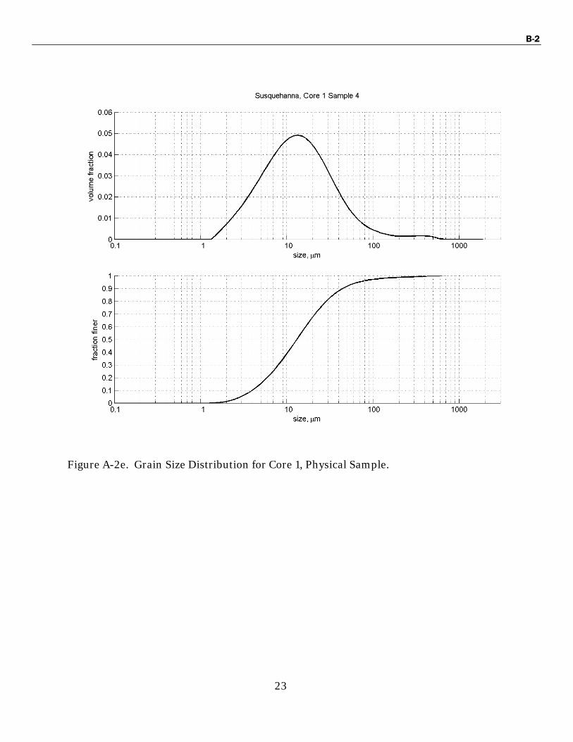
0.00 - 5.08 18.33 74.94 14.10 80.33 5.57
1 0.98 1.28 4.79 15.89 53.64 8.62 85.29 6.09
2 4.25 1.32 4.89 16.22 55.10 9.11 84.99 5.90
3 8.10 1.33 4.46 14.91 59.10 10.12 82.76 7.13
4 11.83 1.33 4.00 13.10 44.72 6.45 84.63 8.92
5 16.15 1.33 4.44 14.74 53.76 8.88 83.94 7.18

B-2
19
Figure A-2a. Grain Size Distribution for Core 1, Physical Sample.

B-2
20
Figure A-2b. Grain Size Distribution for Core 1, Physical Sample.

B-2
21
Figure A-2c. Grain Size Distribution for Core 1, Physical Sample.

B-2
22
Figure A-2d. Grain Size Distribution for Core 1, Physical Sample.
B-2
23
Figure A-2e. Grain Size Distribution for Core 1, Physical Sample.

B-2
24
Figure A-2f. Grain Size Distribution for Core 1, Physical Sample.

B-2
25
Table A-2b. Physical Sample Properties (Core 2c)
Sample
Depth
(cm below
surf)
Bulk den-
sity
(g/cm3)
D10(µm)
D50(µm)
D90(µm)
Percent
Sand
Percent
Silt
Percent
Clay Surface
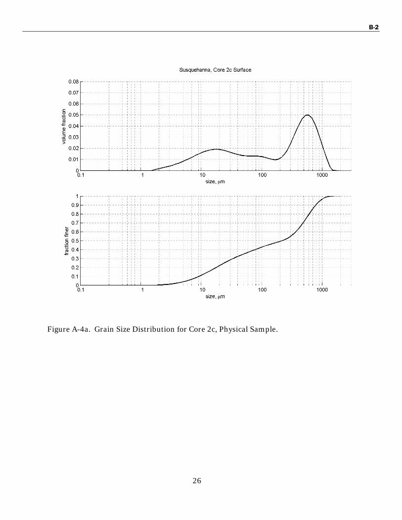
0.00 - 9.24 218.00 787.16 63.38 34.45 2.17
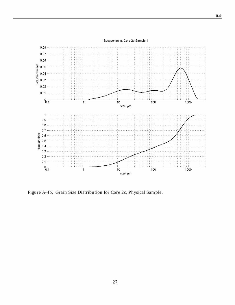
1 1.05 1.42 10.64 294.46 934.12 69.76 28.36 1.88
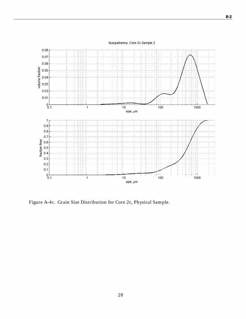
2 4.95 1.62 111.06 545.72 1113.57 95.84 3.95 0.20
3 9.63 1.67 7.71 70.78 589.44 52.74 44.44 2.83
4 13.80 1.38 5.73 23.96 98.95 21.78 73.66 4.56
5 17.30 1.30 5.72 20.25 78.32 15.36 80.31 4.33
6 20.80 1.39 6.00 24.57 103.06 22.36 73.56 4.08
7 25.80 1.38 5.62 22.32 96.57 19.99 75.40 4.62
8 30.60 1.44 6.61 26.44 115.64 24.59 72.17 3.24
9 32.63 1.43 5.27 21.99 96.87 19.85 74.85 5.31
B-2
26
Figure A-4a. Grain Size Distribution for Core 2c, Physical Sample.
B-2
27
Figure A-4b. Grain Size Distribution for Core 2c, Physical Sample.
B-2
28
Figure A-4c. Grain Size Distribution for Core 2c, Physical Sample.

B-2
29
Figure A-4d. Grain Size Distribution for Core 2c, Physical Sample.

B-2
30
Figure A-4e. Grain Size Distribution for Core 2c, Physical Sample.

B-2
31
Figure A-4f. Grain Size Distribution for Core 2c, Physical Sample.

B-2
32
Figure A-4g. Grain Size Distribution for Core 2c, Physical Sample.

B-2
33
Figure A-4h. Grain Size Distribution for Core 2c, Physical Sample.

B-2
34
Figure A-4i. Grain Size Distribution for Core 2c, Physical Sample.

B-2
35
Figure A-4j. Grain Size Distribution for Core 2c, Physical Sample.

B-2
36
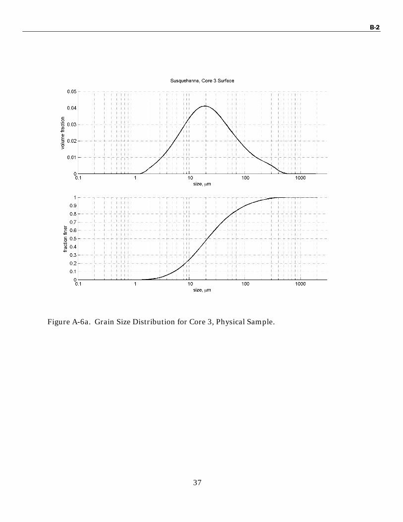
Table A-3b. Physical Sample Properties (Core 3)
Sample
Depth (cm
below
surf)
Bulk den-
sity
(g/cm3)
D10(µm)
D50(µm)
D90(µm)
Percent
Sand
Percent
Silt
Percent
Clay Surface
0.00 - 5.43 21.43 103.07 19.98 75.10 4.92
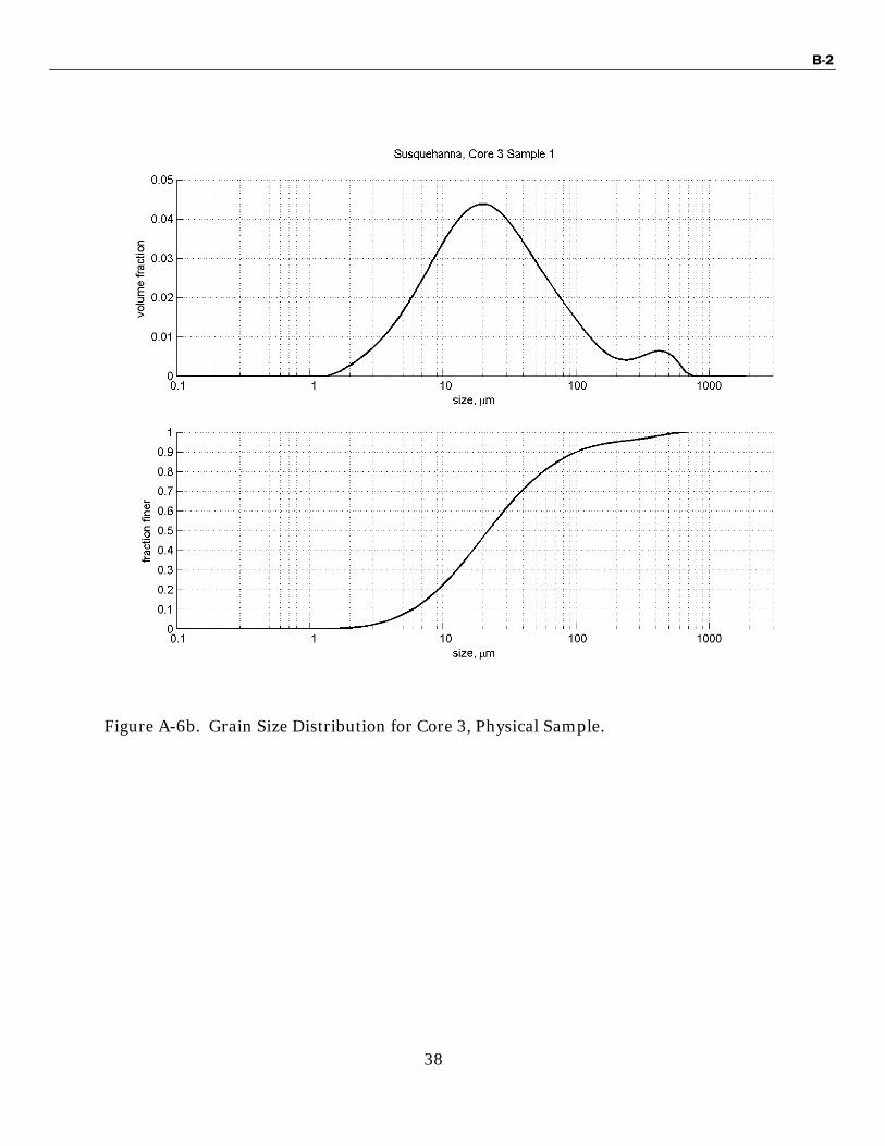
1 0.90 1.29 5.97 21.97 101.41 19.43 76.69 3.89
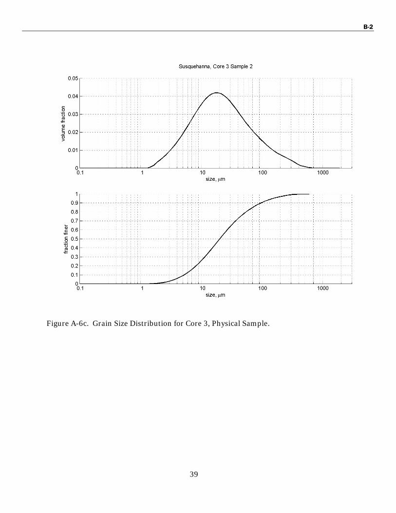
2 4.30 1.34 5.29 20.23 97.87 18.73 76.17 5.09
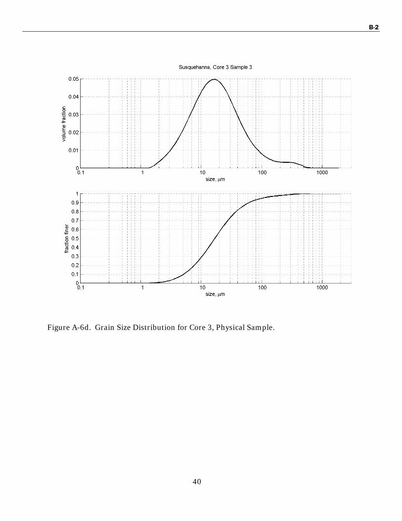
3 8.98 1.36 5.20 16.86 62.54 11.00 84.01 4.99
4 13.40 1.35 4.70 18.65 167.89 24.05 69.55 6.39
5 18.35 1.36 5.62 26.92 192.94 31.32 64.01 4.67
6 23.00 1.36 5.52 23.48 155.38 26.53 68.84 4.63
B-2
37
Figure A-6a. Grain Size Distribution for Core 3, Physical Sample.
B-2
38
Figure A-6b. Grain Size Distribution for Core 3, Physical Sample.
B-2
39
Figure A-6c. Grain Size Distribution for Core 3, Physical Sample.
B-2
40
Figure A-6d. Grain Size Distribution for Core 3, Physical Sample.

B-2
41
Figure A-6e. Grain Size Distribution for Core 3, Physical Sample.

B-2
42
Figure A-6f. Grain Size Distribution for Core 3, Physical Sample.
B-2
43
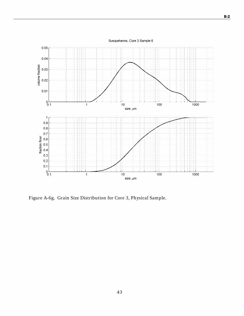
Figure A-6g. Grain Size Distribution for Core 3, Physical Sample.

B-2
44
Table A-4b. Physical Sample Properties (Core 4)
Sample
Depth
(cm below
surf)
Bulk den-
sity
(g/cm3)
D10(µm)
D50(µm)
D90(µm)
Percent
Sand
Percent
Silt
Percent
Clay Surface
0.00 - 5.57 21.01 85.43 17.29 78.03 4.69
1 0.88 1.43 5.56 29.41 98.38 24.59 70.36 5.05
2 4.05 1.33 4.97 20.55 124.06 21.77 72.33 5.90
3 8.55 1.40 4.67 15.82 56.06 9.37 84.13 6.50
4 13.10 1.46 4.34 15.84 68.63 12.43 79.99 7.58
B-2
45
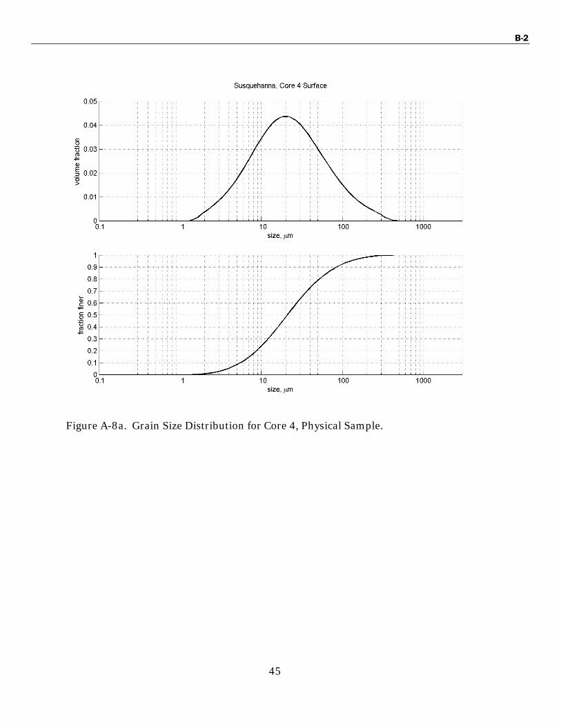
Figure A-8a. Grain Size Distribution for Core 4, Physical Sample.
B-2
46
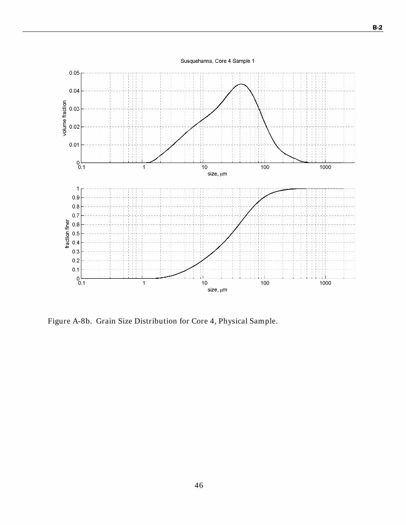
Figure A-8b. Grain Size Distribution for Core 4, Physical Sample.

B-2
47
Figure A-8c. Grain Size Distribution for Core 4, Physical Sample.

B-2
48
Figure A-8d. Grain Size Distribution for Core 4, Physical Sample.
B-2
49
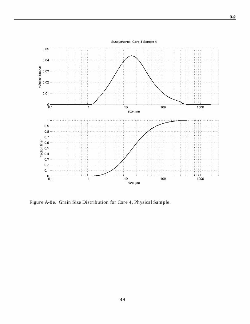
Figure A-8e. Grain Size Distribution for Core 4, Physical Sample.
B-2
50
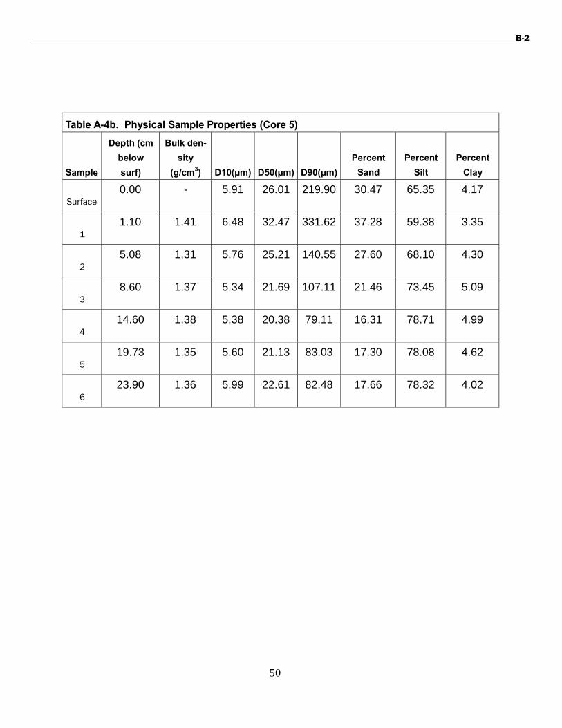
Table A-4b. Physical Sample Properties (Core 5)
Sample
Depth (cm
below
surf)
Bulk den-
sity
(g/cm3)
D10(µm)
D50(µm)
D90(µm)
Percent
Sand
Percent
Silt
Percent
Clay Surface
0.00 - 5.91 26.01 219.90 30.47 65.35 4.17
1 1.10 1.41 6.48 32.47 331.62 37.28 59.38 3.35
2 5.08 1.31 5.76 25.21 140.55 27.60 68.10 4.30
3 8.60 1.37 5.34 21.69 107.11 21.46 73.45 5.09
4 14.60 1.38 5.38 20.38 79.11 16.31 78.71 4.99
5 19.73 1.35 5.60 21.13 83.03 17.30 78.08 4.62
6 23.90 1.36 5.99 22.61 82.48 17.66 78.32 4.02

B-2
51
Figure A-10a. Grain Size Distribution for Core 5, Physical Sample.
B-2
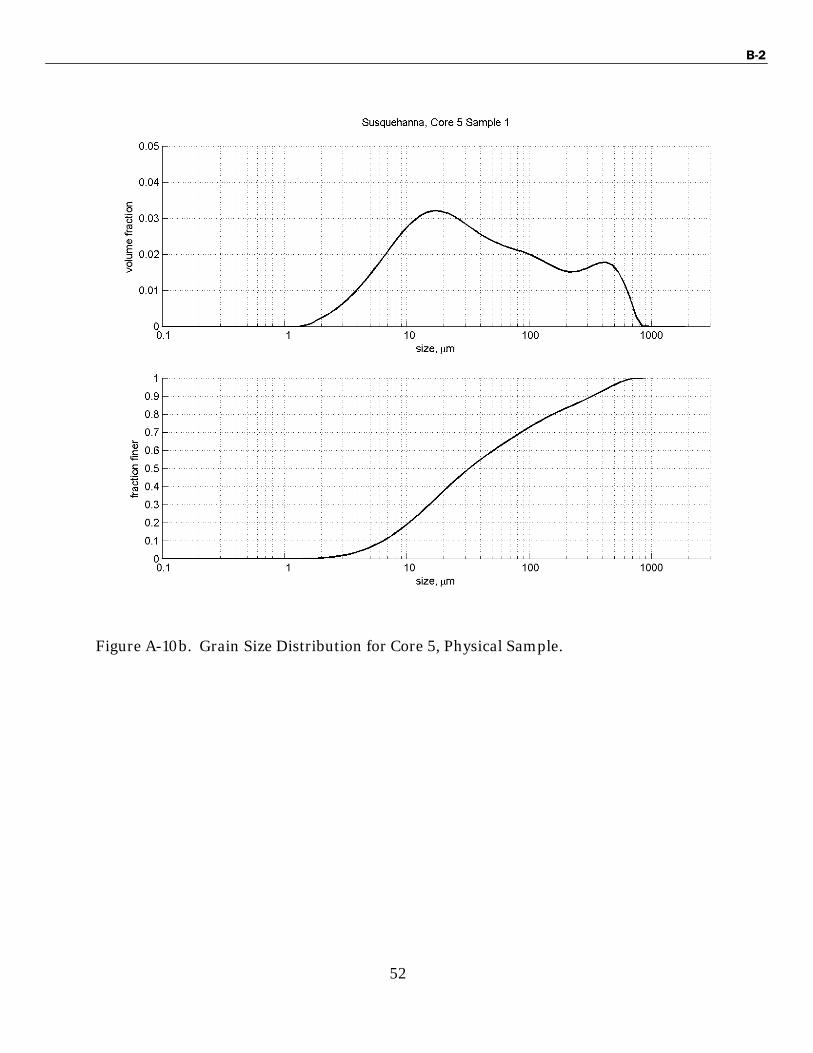
52
Figure A-10b. Grain Size Distribution for Core 5, Physical Sample.

B-2
53
Figure A-10c. Grain Size Distribution for Core 5, Physical Sample.

B-2
54
Figure A-10d. Grain Size Distribution for Core 5, Physical Sample.

B-2
55
Figure A-10e. Grain Size Distribution for Core 5, Physical Sample.

B-2
56
Figure A-10f. Grain Size Distribution for Core 5, Physical Sample.

B-2
57
Figure A-10g. Grain Size Distribution for Core 5, Physical Sample.

B-2
58
Table A-6b. Physical Sample Properties (Core 6)
Sample
Depth
(cm below
surf)
Bulk den-
sity
(g/cm3)
D10(µm)
D50(µm)
D90(µm)
Percent
Sand
Percent
Silt
Percent
Clay Surface
0.00 - 7.82 159.13 450.74 56.59 40.68 2.74
1 1.60 1.53 4.41 19.90 197.12 24.45 68.07 7.48
2 5.43 1.46 4.72 22.68 124.51 25.69 67.79 6.52
3 10.25 1.52 5.62 30.94 156.51 32.98 62.15 4.87
4 13.95 1.57 5.62 30.73 168.99 34.46 60.79 4.75

B-2
59
Figure A-12a. Grain Size Distribution for Core 6, Physical Sample.
B-2
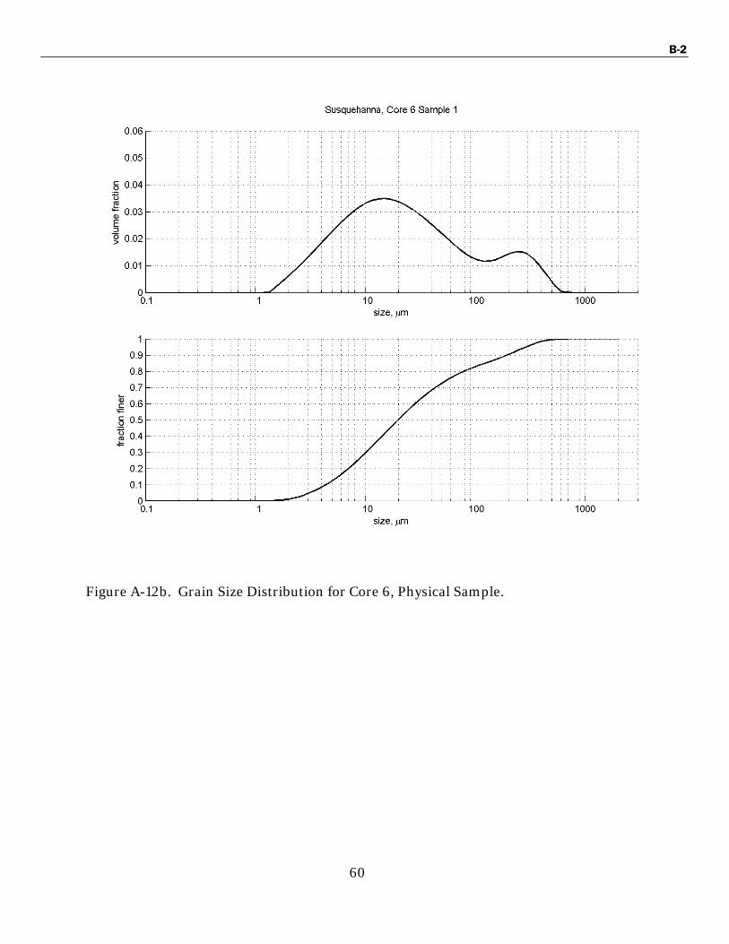
60
Figure A-12b. Grain Size Distribution for Core 6, Physical Sample.

B-2
61
Figure A-12c. Grain Size Distribution for Core 6, Physical Sample.

B-2
62
Figure A-12d. Grain Size Distribution for Core 6, Physical Sample.

B-2
63
Figure A-12e. Grain Size Distribution for Core 6, Physical Sample.
B-2
64
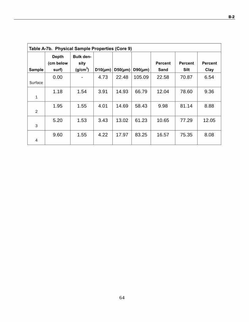
Table A-7b. Physical Sample Properties (Core 9)
Sample
Depth
(cm below
surf)
Bulk den-
sity
(g/cm3)
D10(µm)
D50(µm)
D90(µm)
Percent
Sand
Percent
Silt
Percent
Clay Surface
0.00 - 4.73 22.48 105.09 22.58 70.87 6.54
1 1.18 1.54 3.91 14.93 66.79 12.04 78.60 9.36
2 1.95 1.55 4.01 14.69 58.43 9.98 81.14 8.88
3 5.20 1.53 3.43 13.02 61.23 10.65 77.29 12.05
4 9.60 1.55 4.22 17.97 83.25 16.57 75.35 8.08

B-2
65
Figure A-14a. Grain Size Distribution for Core 9, Physical Sample.
B-2
66
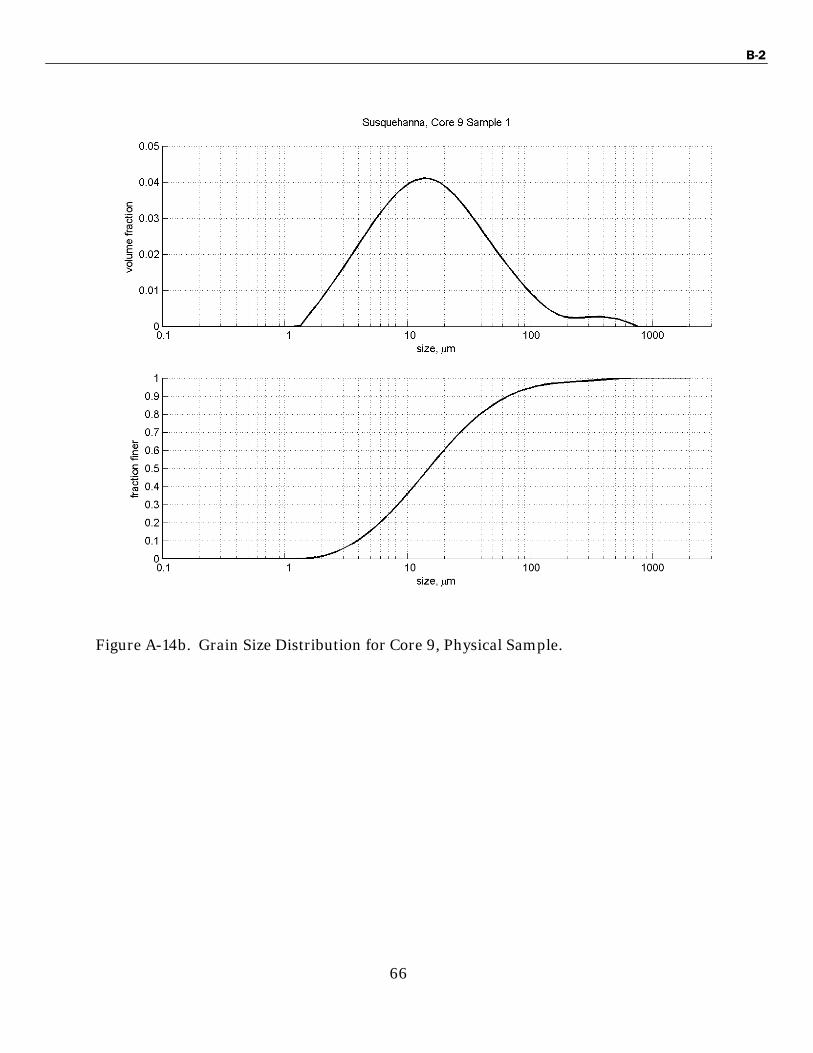
Figure A-14b. Grain Size Distribution for Core 9, Physical Sample.

B-2
67
Figure A-14c. Grain Size Distribution for Core 9, Physical Sample.

B-2
68
Figure A-14d. Grain Size Distribution for Core 9, Physical Sample.

B-2
69
Figure A-14e. Grain Size Distribution for Core 9, Physical Sample.
B-2
70
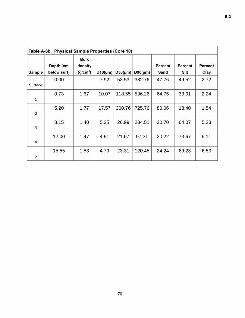
Table A-8b. Physical Sample Properties (Core 10) Sample
Depth (cm
below surf)
Bulk
density
(g/cm3)
D10(µm)
D50(µm)
D90(µm)
Percent
Sand
Percent
Silt
Percent
Clay Surface
0.00 - 7.92 53.53 382.76 47.76 49.52 2.72
1 0.73 1.67 10.07 118.55 536.26 64.75 33.01 2.24
2 5.20 1.77 17.57 300.76 725.76 80.06 18.40 1.54
3 8.15 1.40 5.35 26.99 234.51 30.70 64.07 5.23
4 12.00 1.47 4.91 21.67 97.31 20.22 73.67 6.11
5 15.55 1.53 4.79 23.31 120.45 24.24 69.23 6.53

B-2
71
Figure A-15a. Grain Size Distribution for Core 10, Physical Sample.

B-2
72
Figure A-15b. Grain Size Distribution for Core 10, Physical Sample.
B-2
73
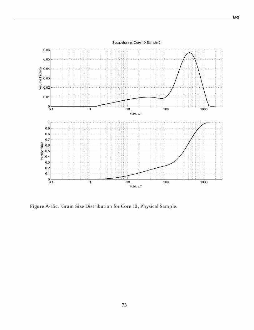
Figure A-15c. Grain Size Distribution for Core 10, Physical Sample.

B-2
74
Figure A-15d. Grain Size Distribution for Core 10, Physical Sample.

B-2
75
Figure A-15e. Grain Size Distribution for Core 10, Physical Sample.

B-2
76
Figure A-15f. Grain Size Distribution for Core 10, Physical Sample.

B-2
77
Erosion versus Depth
Figure B-1. Erosion versus depth for core 1. Colors indicate bed layers, symbols indicate applied shear stress.

B-2
78
Figure B-2. Erosion versus depth for core 2. Colors indicate bed layers, symbols indicate applied shear stress.

B-2
79
Figure B-3. Erosion versus depth for core 3. Colors indicate bed layers, symbols indicate applied shear stress.

B-2
80
Figure B-4. Erosion versus depth for core 4. Colors indicate bed layers, symbols indicate applied shear stress.

B-2
81
Figure B-5. Erosion versus depth for core 5. Colors indicate bed layers, symbols indicate applied shear stress.

B-2
82
Figure B-6. Erosion versus depth for core 6. Colors indicate bed layers, symbols indicate applied shear stress.

B-2
83
Figure B-7. Erosion versus depth for core 9. Colors indicate bed layers, symbols indicate applied shear stress.

B-2
84
Figure B-8. Erosion versus depth for core 10. Colors indicate bed layers, symbols indicate applied shear stress.

B-2
85
Erosion versus shear stress (Partheniades)
Core 1
Table B-1. Cohesive Sediment Erosion Parameterization
Layer ID
Depth (cm)
Critical Shear
(τcr)
Erosion Rate
Constant (M)
Erosion Rate Ex-
ponent (n)
Pa - -
Core01_L1 0-4 0.20 2.02E-02 1.14
Core01_L2 5-10 0.40 2.89E-02 1.10
Core01_L3 10-14 0.80 3.52E-02 0.96

B-2
86
Figure B-9. Erosion versus applied shear stress for core 1, Layer 1. Colors indicate bed layers, Lines represent best-fit line to Partheniades’ erosion function. Erosion equation parameters provided at top of figure.

B-2
87
Figure B-10. Erosion versus applied shear stress for core 1, Layer 2. Colors indicate bed layers, Lines represent best-fit line to Partheniades’ erosion function. Erosion equation parameters pro- vided at top of figure.

B-2
88
Figure B-11. Erosion versus applied shear stress for core 1, Layer 3. Colors indicate bed layers, Lines represent best-fit line to Partheniades’ erosion function. Erosion equation parameters provid- ed at top of figure.

B-2
89
Core 2
Table B-2. Cohesive Sediment Erosion Parameterization
Layer ID
Depth (cm)
Critical Shear
(τcr)
Erosion Rate
Constant (M)
Erosion Rate Ex-
ponent (n)
Pa - -
Core02_L1 0-10 0.20 1.01E-01 1.05
Core02_L2 10-17 0.40 5.98E-02 1.52
Core02_L3 17-24 0.80 3.73E-02 1.36
Core02_L4 24-32 1.60 9.18E-02 0.92
Core02_L3&4 17-32 0.80 3.86E-02 0.92

B-2
90
Figure B-12. Erosion versus applied shear stress for core 2, Layer 1. Colors indicate bed layers, Lines represent best-fit line to Partheniades’ erosion function. Erosion equation parameters provided at top of figure.
B-2
91
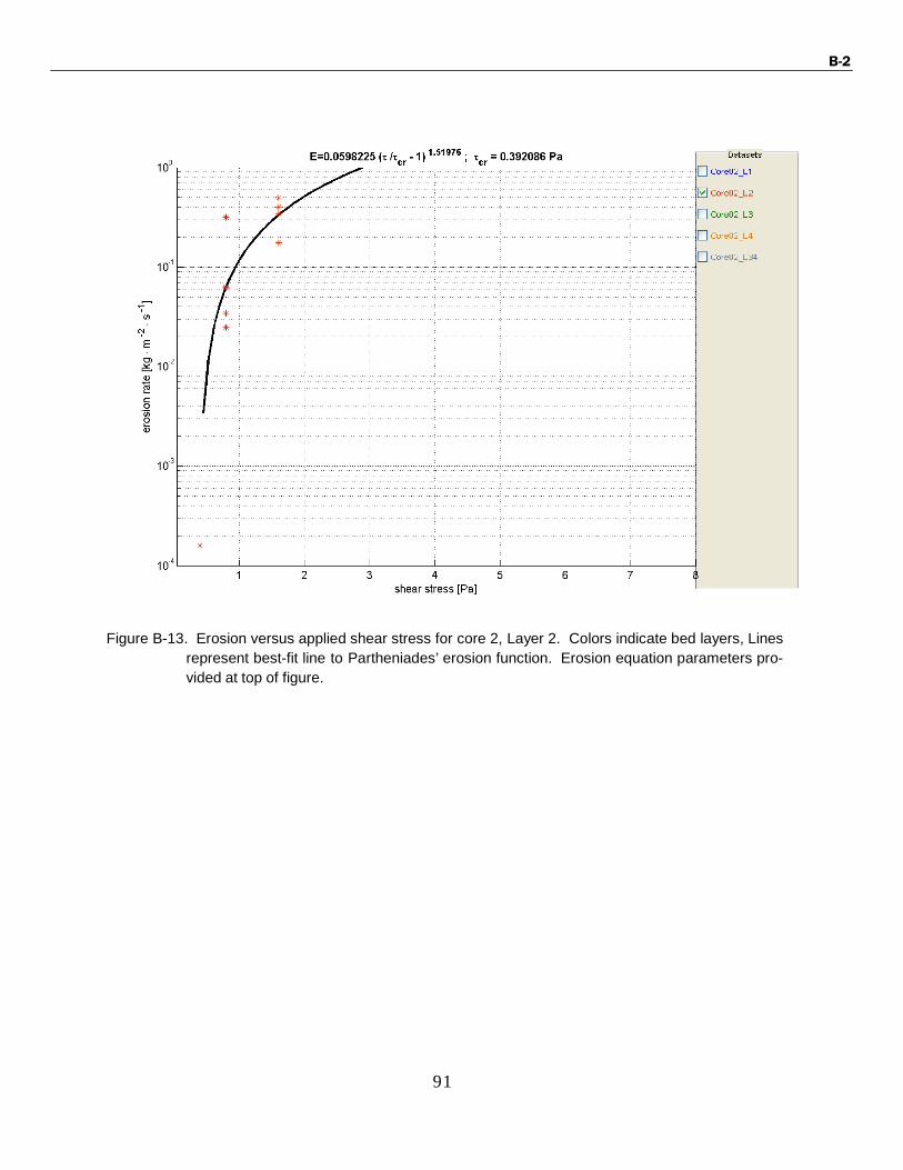
Figure B-13. Erosion versus applied shear stress for core 2, Layer 2. Colors indicate bed layers, Lines represent best-fit line to Partheniades’ erosion function. Erosion equation parameters pro- vided at top of figure.
B-2
92
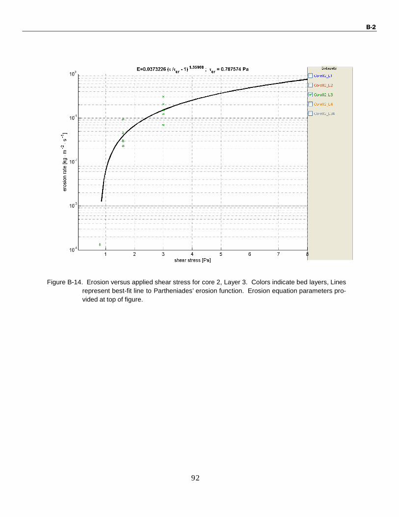
Figure B-14. Erosion versus applied shear stress for core 2, Layer 3. Colors indicate bed layers, Lines represent best-fit line to Partheniades’ erosion function. Erosion equation parameters pro- vided at top of figure.

B-2
93
Figure B-15. Erosion versus applied shear stress for core 2, Layer 4. Colors indicate bed layers, Lines represent best-fit line to Partheniades’ erosion function. Erosion equation parameters pro- vided at top of figure.

B-2
94
Figure B-16. Erosion versus applied shear stress for core 2, Layer 3 and Layer 4. Colors indicate bed layers, Lines represent best-fit line to Partheniades’ erosion function. Erosion equation pa- rameters provided at top of figure.

B-2
95
Core 3
Table B-3. Cohesive Sediment Erosion Parameterization
Layer ID
Depth (cm)
Critical Shear
(τcr)
Erosion Rate
Constant (M)
Erosion Rate Ex-
ponent (n)
Pa - -
Core03_L1 0-2.5 0.20 9.90E-03 0.98
Core03_L2 2.5-22 0.80 8.08E-02 1.00
B-2
96
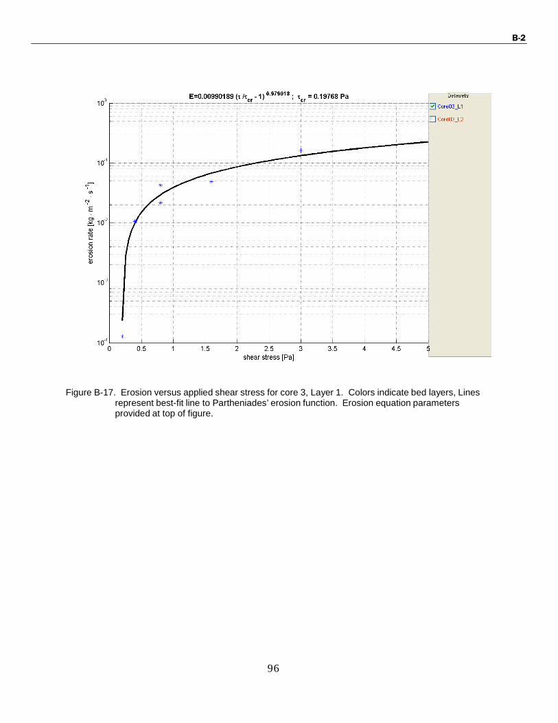
Figure B-17. Erosion versus applied shear stress for core 3, Layer 1. Colors indicate bed layers, Lines represent best-fit line to Partheniades’ erosion function. Erosion equation parameters provided at top of figure.

B-2
97
Figure B-18. Erosion versus applied shear stress for core 3, Layer 2. Colors indicate bed layers, Lines represent best-fit line to Partheniades’ erosion function. Erosion equation parameters pro- vided at top of figure.

B-2
98
Core 4
Table B-4. Cohesive Sediment Erosion Parameterization
Layer ID
Depth (cm)
Critical Shear
(τcr)
Erosion Rate
Constant (M)
Erosion Rate Ex-
ponent (n)
Pa - -
Core04_L1 0-2 0.20 1.04E-02 1.21
Core04_L2 2-11 0.80 3.23E-02 0.90

B-2
99
Figure B-19. Erosion versus applied shear stress for core 4, Layer 1. Colors indicate bed layers, Lines represent best-fit line to Partheniades’ erosion function. Erosion equation parameters provided at top of figure.
B-2
100
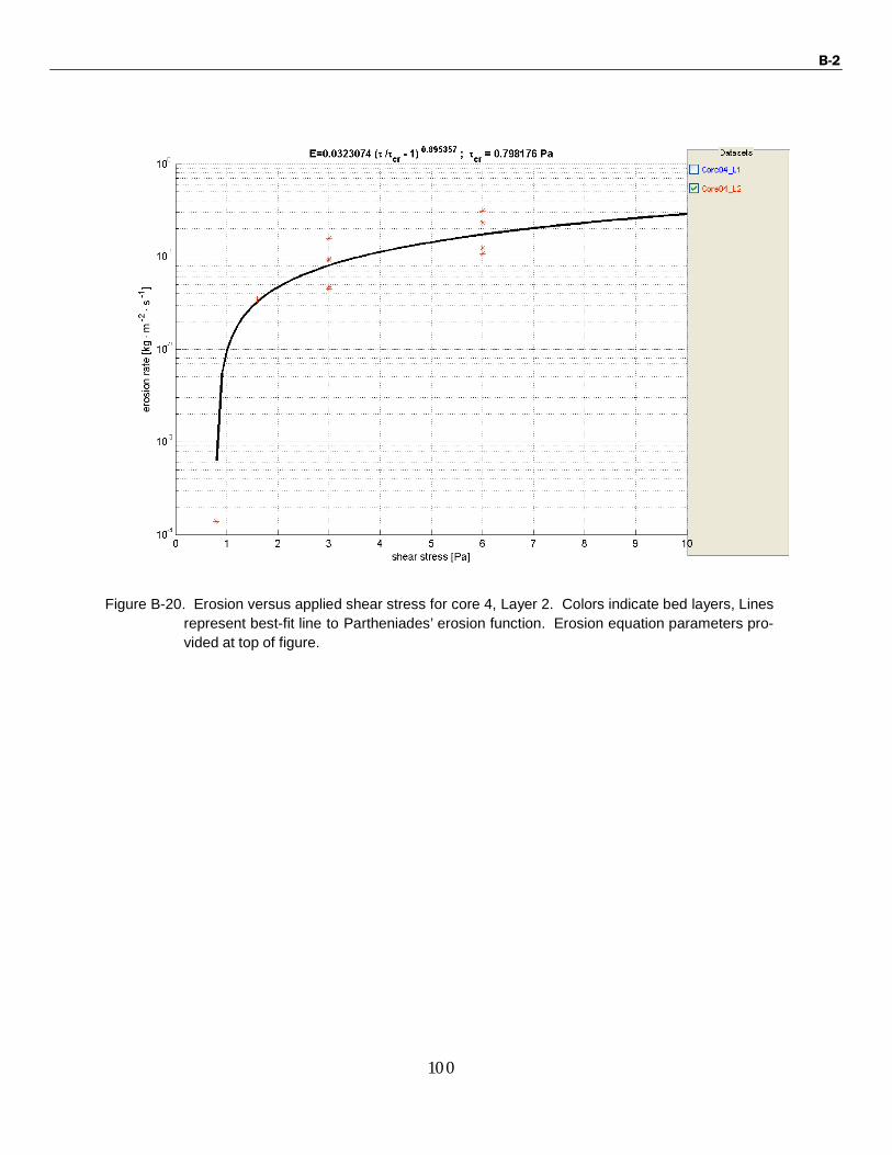
Figure B-20. Erosion versus applied shear stress for core 4, Layer 2. Colors indicate bed layers, Lines represent best-fit line to Partheniades’ erosion function. Erosion equation parameters pro- vided at top of figure.
B-2
101
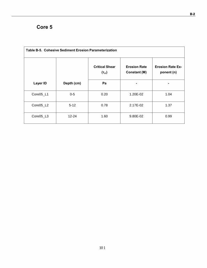
Core 5
Table B-5. Cohesive Sediment Erosion Parameterization
Layer ID
Depth (cm)
Critical Shear
(τcr)
Erosion Rate
Constant (M)
Erosion Rate Ex-
ponent (n)
Pa - -
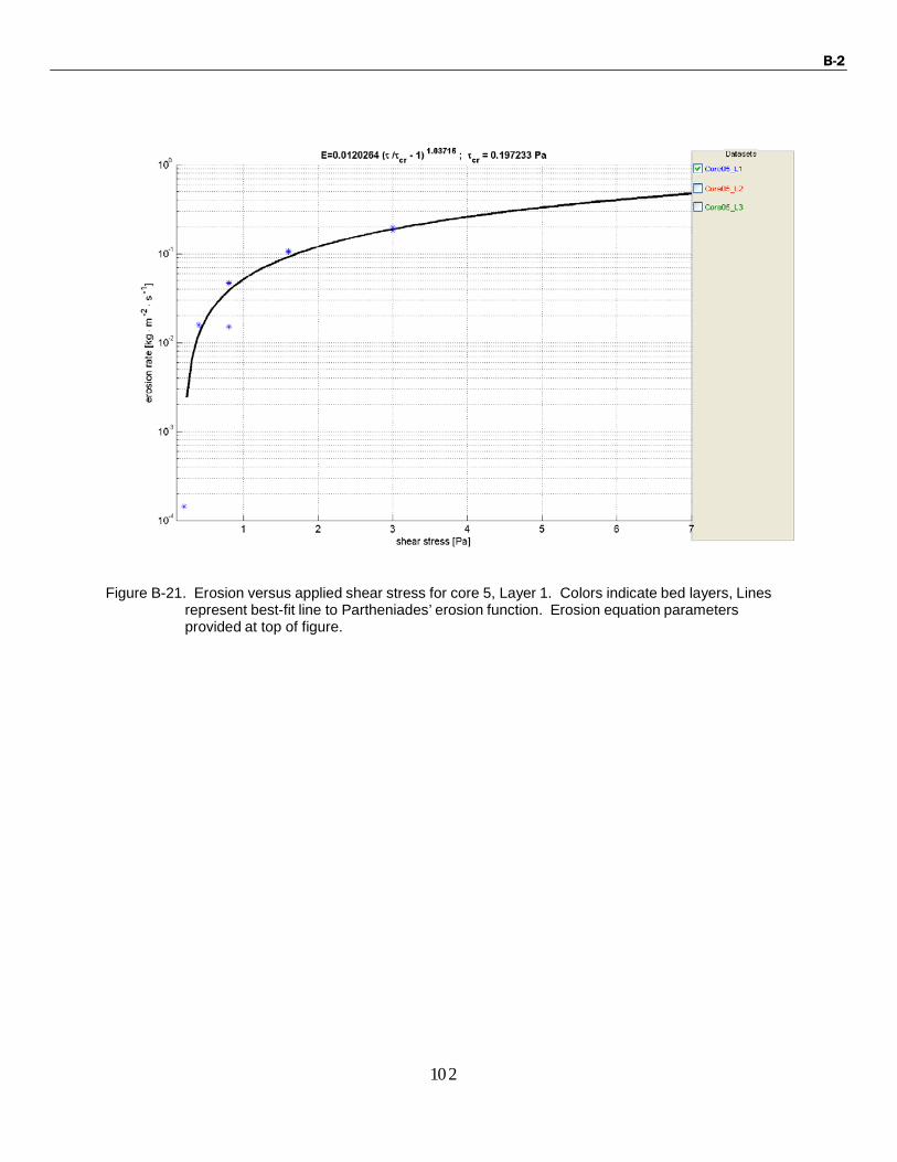
Core05_L1 0-5 0.20 1.20E-02 1.04
Core05_L2 5-12 0.78 2.17E-02 1.37
Core05_L3 12-24 1.60 9.80E-02 0.99
B-2
102
Figure B-21. Erosion versus applied shear stress for core 5, Layer 1. Colors indicate bed layers, Lines represent best-fit line to Partheniades’ erosion function. Erosion equation parameters provided at top of figure.

B-2
103
Figure B-22. Erosion versus applied shear stress for core 5, Layer 2. Colors indicate bed layers, Lines represent best-fit line to Partheniades’ erosion function. Erosion equation parameters pro- vided at top of figure.

B-2
104
Figure B-23. Erosion versus applied shear stress for core 5, Layer 3. Colors indicate bed layers, Lines represent best-fit line to Partheniades’ erosion function. Erosion equation parameters provided at top of figure.

B-2
105
Core 6
Table B-6. Cohesive Sediment Erosion Parameterization
Layer ID
Depth (cm)
Critical Shear
(τcr)
Erosion Rate
Constant (M)
Erosion Rate Ex-
ponent (n)
Pa - -
Core06_L1 0-2 0.10 1.48E-02 0.90
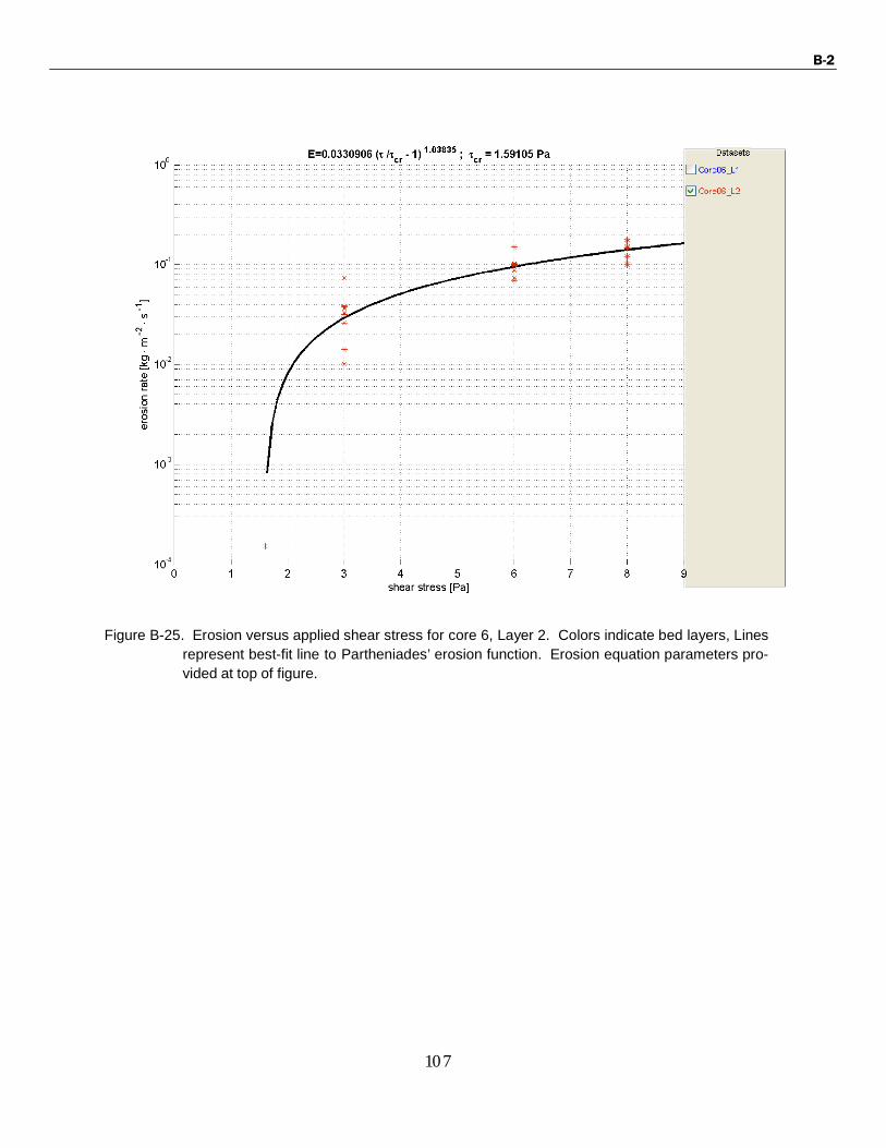
Core06_L2 2-14 1.60 3.31E-02 1.04

B-2
106
Figure B-24. Erosion versus applied shear stress for core 6, Layer 1. Colors indicate bed layers, Lines represent best-fit line to Partheniades’ erosion function. Erosion equation parameters provided at top of figure.
B-2
107
Figure B-25. Erosion versus applied shear stress for core 6, Layer 2. Colors indicate bed layers, Lines represent best-fit line to Partheniades’ erosion function. Erosion equation parameters pro- vided at top of figure.

B-2
108
Core 9
Table B-7. Cohesive Sediment Erosion Parameterization
Layer ID
Depth (cm)
Critical Shear
(τcr)
Erosion Rate
Constant (M)
Erosion Rate Ex-
ponent (n)
Pa - -
Core09_L1 0-2 0.20 8.20E-03 1.41
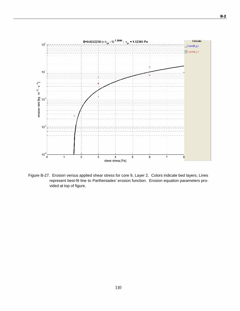
Core09_L2 2-9 1.52 2.32E-02 1.36

B-2
109
Figure B-26. Erosion versus applied shear stress for core 9, Layer 1. Colors indicate bed layers, Lines represent best-fit line to Partheniades’ erosion function. Erosion equation parameters provided at top of figure.
B-2
110
Figure B-27. Erosion versus applied shear stress for core 9, Layer 2. Colors indicate bed layers, Lines represent best-fit line to Partheniades’ erosion function. Erosion equation parameters pro- vided at top of figure.

B-2
111
Core 10
Table B-8. Cohesive Sediment Erosion Parameterization
Layer ID
Depth (cm)
Critical Shear
(τcr)
Erosion Rate
Constant (M)
Erosion Rate Ex-
ponent (n)
Pa - -
Core10_L1 0-8 0.18 3.40E-02 1.31
Core10_L2 8-16 1.14 1.70E-02 1.61

B-2
112
Figure B-28. Erosion versus applied shear stress for core 10, Layer 1. Colors indicate bed layers, Lines represent best-fit line to Partheniades’ erosion function. Erosion equation parameters provided at top of figure.

B-2
113
Figure B-29. Erosion versus applied shear stress for core 10, Layer 2. Colors indicate bed layers, Lines represent best-fit line to Partheniades’ erosion function. Erosion equation parameters pro- vided at top of figure.

B-2
114
Erosion versus shear stress (HEC-RAS fit to Partheniades)
Core 1
Table B-9. Cohesive Sediment Erosion Parameterization for HEC-RAS
Layer ID
Depth
(cm)
Shear Thresh-
old
Erosion Rate
Mass Wasting
Threshold
Mass Wasting
Rate
Pa lb/ft2 kg/m2/s lb/ft2/hr Pa lb/ft2
kg/m2/s lb/ft2/hr
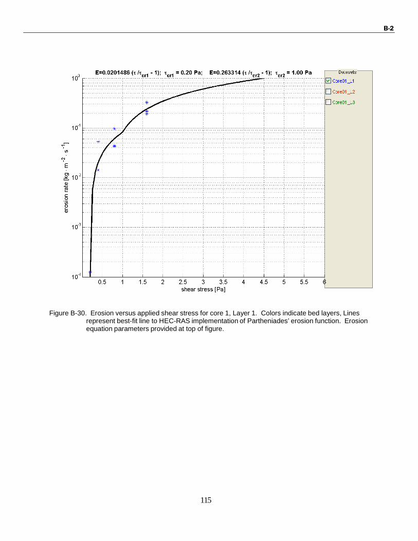
Core01_L1 0-4 0.2 0.0042 2.02E-02 14.9 1 0.0209 0.263 193.9
Core01_L2 5-14 0.4 0.0084 3.24E-02 23.9 - - - -
Core01_L3 10-14 0.8 0.0167 3.39E-02 25.0 - - - -
B-2
115
Figure B-30. Erosion versus applied shear stress for core 1, Layer 1. Colors indicate bed layers, Lines represent best-fit line to HEC-RAS implementation of Partheniades’ erosion function. Erosion equation parameters provided at top of figure.

B-2
116
Figure B-31. Erosion versus applied shear stress for core 1, Layer 2. Colors indicate bed layers, Lines
represent best-fit line to HEC-RAS implementation of Partheniades’ erosion function. Erosion
equation parameters provided at top of figure.

B-2
117
Figure B-32. Erosion versus applied shear stress for core 1, Layer 3. Colors indicate bed layers, Lines
represent best-fit line to HEC-RAS implementation of Partheniades’ erosion function. Erosion
equation parameters provided at top of figure.
B-2
118
Core 2
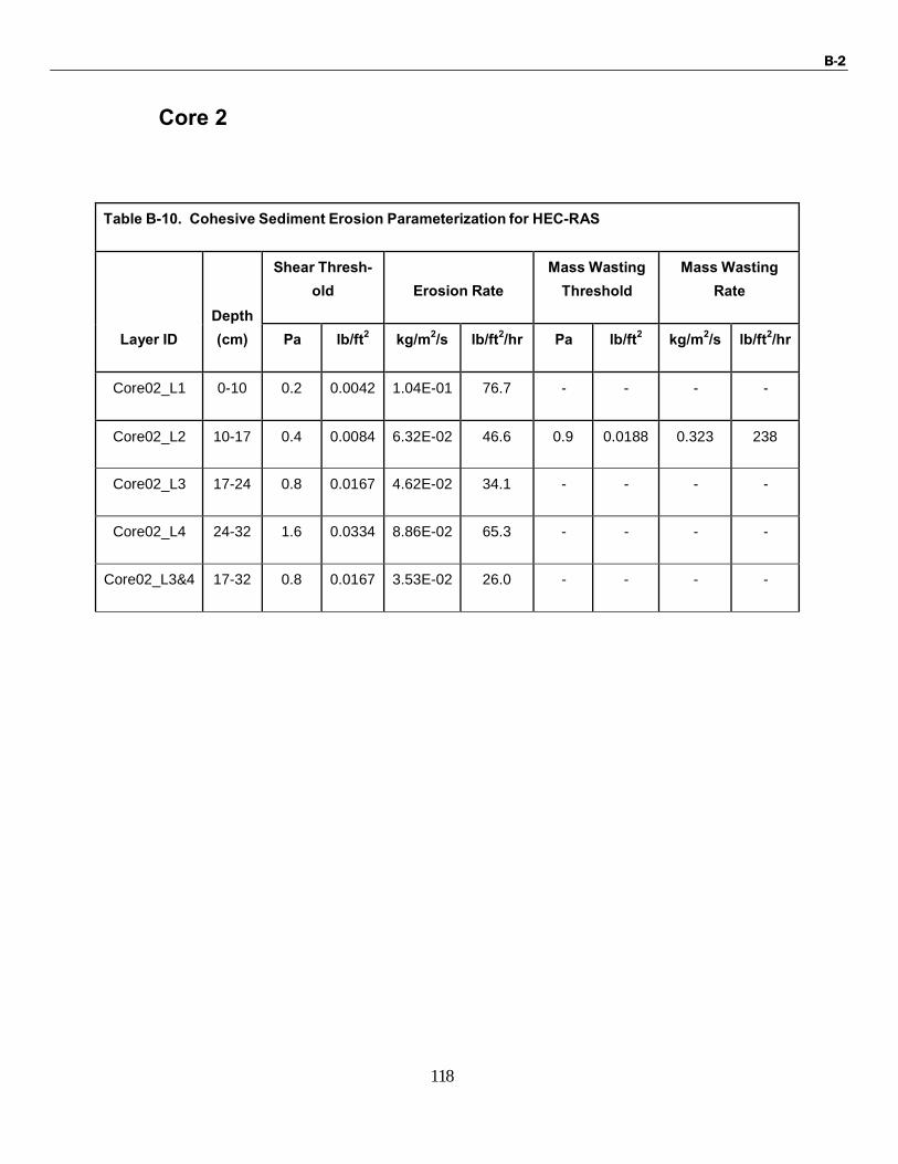
Table B-10. Cohesive Sediment Erosion Parameterization for HEC-RAS
Layer ID
Depth
(cm)
Shear Thresh-
old
Erosion Rate
Mass Wasting
Threshold
Mass Wasting
Rate
Pa lb/ft2 kg/m2/s lb/ft2/hr Pa lb/ft2
kg/m2/s lb/ft2/hr
Core02_L1 0-10 0.2 0.0042 1.04E-01 76.7 - - - -
Core02_L2 10-17 0.4 0.0084 6.32E-02 46.6 0.9 0.0188 0.323 238
Core02_L3 17-24 0.8 0.0167 4.62E-02 34.1 - - - -
Core02_L4 24-32 1.6 0.0334 8.86E-02 65.3 - - - -
Core02_L3&4 17-32 0.8 0.0167 3.53E-02 26.0 - - - -
B-2
119
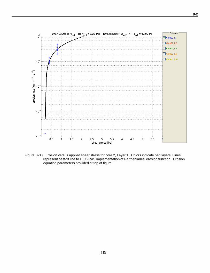
Figure B-33. Erosion versus applied shear stress for core 2, Layer 1. Colors indicate bed layers, Lines represent best-fit line to HEC-RAS implementation of Partheniades’ erosion function. Erosion equation parameters provided at top of figure.
B-2
120
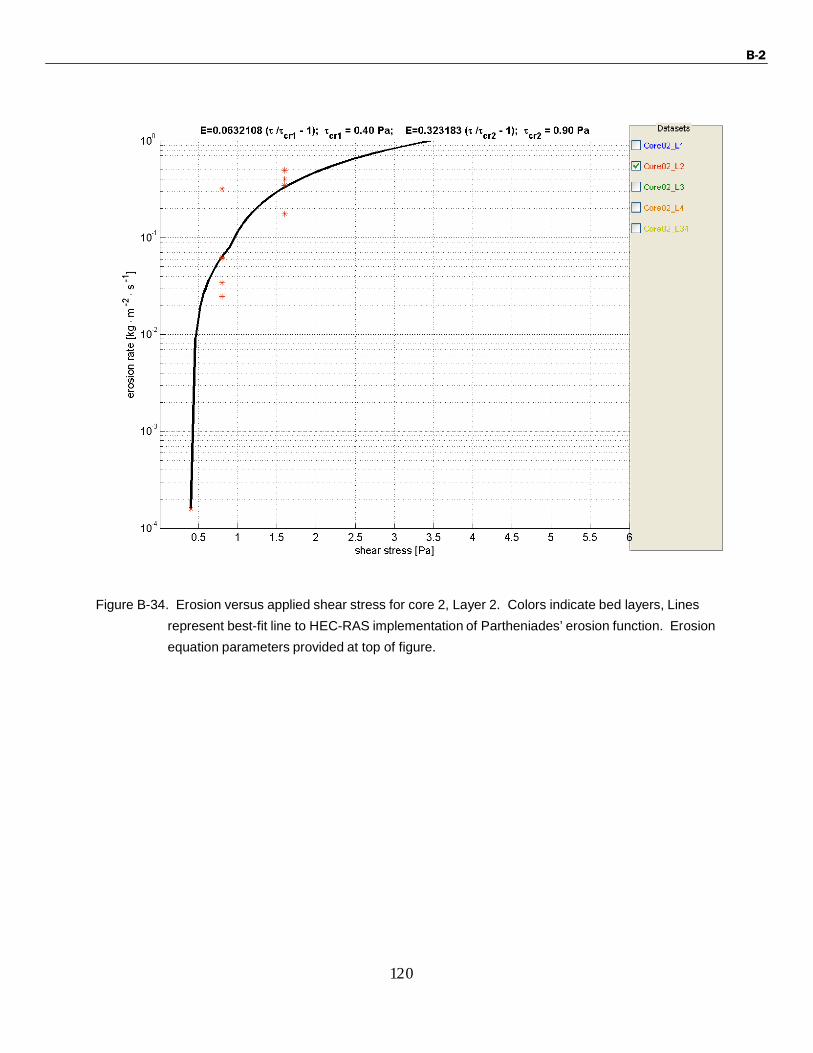
Figure B-34. Erosion versus applied shear stress for core 2, Layer 2. Colors indicate bed layers, Lines
represent best-fit line to HEC-RAS implementation of Partheniades’ erosion function. Erosion
equation parameters provided at top of figure.

B-2
121
Figure B-35. Erosion versus applied shear stress for core 2, Layer 3. Colors indicate bed layers, Lines
represent best-fit line to HEC-RAS implementation of Partheniades’ erosion function. Erosion
equation parameters provided at top of figure.

B-2
122
Figure B-36. Erosion versus applied shear stress for core 2, Layer 4. Colors indicate bed layers, Lines
represent best-fit line to HEC-RAS implementation of Partheniades’ erosion function. Erosion
equation parameters provided at top of figure.

B-2
123
Figure B-37. Erosion versus applied shear stress for core 2, Layer 3 and Layer 4. Colors indicate bed
layers, Lines represent best-fit line to HEC-RAS implementation of Partheniades’ erosion
function. Erosion equation parameters provided at top of figure.

B-2
124
Core 3
Table B-11. Cohesive Sediment Erosion Parameterization for HEC-RAS
Layer ID
Depth
(cm)
Shear Thresh-
old
Erosion Rate
Mass Wasting
Threshold
Mass Wasting
Rate
Pa lb/ft2 kg/m2/s lb/ft2/hr Pa lb/ft2
kg/m2/s lb/ft2/hr
Core03_L1 0-2.5 0.2 0.0042 9.60E-03 7.08 - - - -
Core03_L2 2.5-22 0.8 0.0167 8.07E-02 59.5 - - - -
Core03_L1&2 0-22 0.2 0.0042 1.09E-02 8.04 2 0.0418 0.237 175

B-2
125
Figure B-38. Erosion versus applied shear stress for core 3, Layer 1. Colors indicate bed layers, Lines represent best-fit line to HEC-RAS implementation of Partheniades’ erosion function. Erosion equation parameters provided at top of figure.

B-2
126
Figure B-39. Erosion versus applied shear stress for core 3, Layer 2. Colors indicate bed layers, Lines
represent best-fit line to HEC-RAS implementation of Partheniades’ erosion function. Erosion
equation parameters provided at top of figure.

B-2
127
Figure B-40. Erosion versus applied shear stress for core 3, Layer 1 and Layer 2. Colors indicate bed
layers, Lines represent best-fit line to HEC-RAS implementation of Partheniades’ erosion
function. Erosion equation parameters provided at top of figure.

B-2
128
Core 4
Table B-12. Cohesive Sediment Erosion Parameterization for HEC-RAS
Layer ID
Depth
(cm)
Shear Thresh-
old
Erosion Rate
Mass Wasting
Threshold
Mass Wasting
Rate
Pa lb/ft2 kg/m2/s lb/ft2/hr Pa lb/ft2
kg/m2/s lb/ft2/hr
Core04_L1 0-2 0.2 0.0042 1.20E-02 8.85 0.8 0.0167 0.087 64.1
Core04_L2 2-11 0.8 0.0167 2.82E-02 20.8 - - - -

B-2
129
Figure B-41. Erosion versus applied shear stress for core 4, Layer 1. Colors indicate bed layers, Lines represent best-fit line to HEC-RAS implementation of Partheniades’ erosion function. Erosion equation parameters provided at top of figure.

B-2
130
Figure B-42. Erosion versus applied shear stress for core 4, Layer 2. Colors indicate bed layers, Lines
represent best-fit line to HEC-RAS implementation of Partheniades’ erosion function. Erosion
equation parameters provided at top of figure.

B-2
131
Core 5
Table B-13. Cohesive Sediment Erosion Parameterization for HEC-RAS
Layer ID
Depth
(cm)
Shear Thresh-
old
Erosion Rate
Mass Wasting
Threshold
Mass Wasting
Rate
Pa lb/ft2 kg/m2/s lb/ft2/hr Pa lb/ft2
kg/m2/s lb/ft2/hr
Core05_L1 0-5 0.2 0.0042 1.28E-02 9.44 - - - -
Core05_L2 5-12 0.8 0.0167 2.22E-02 16.4 2 0.0418 0.125 92.2
Core05_L3 12-24 1.6 0.0334 9.76E-02 72.0 - - - -

B-2
132
Figure B-43. Erosion versus applied shear stress for core 5, Layer 1. Colors indicate bed layers, Lines represent best-fit line to HEC-RAS implementation of Partheniades’ erosion function. Erosion equation parameters provided at top of figure.

B-2
133
Figure B-44. Erosion versus applied shear stress for core 5, Layer 2. Colors indicate bed layers, Lines
represent best-fit line to HEC-RAS implementation of Partheniades’ erosion function. Erosion
equation parameters provided at top of figure.

B-2
134
Figure B-45. Erosion versus applied shear stress for core 5, Layer 3. Colors indicate bed layers, Lines
represent best-fit line to HEC-RAS implementation of Partheniades’ erosion function. Erosion
equation parameters provided at top of figure.

B-2
135
Core 6
Table B-14. Cohesive Sediment Erosion Parameterization for HEC-RAS
Layer ID
Depth
(cm)
Shear Thresh-
old
Erosion Rate
Mass Wasting
Threshold
Mass Wasting
Rate
Pa lb/ft2 kg/m2/s lb/ft2/hr Pa lb/ft2
kg/m2/s lb/ft2/hr
Core06_L1 0-2 0.1 0.0021 1.32E-02 9.73 - - - -
Core06_L2 2-14 1.59 0.0332 3.41E-02 25.1 - - - -

B-2
136
Figure B-46. Erosion versus applied shear stress for core 6, Layer 1. Colors indicate bed layers, Lines represent best-fit line to Partheniades’ erosion function. Erosion equation parameters provided at top of figure.

B-2
137
Figure B-47. Erosion versus applied shear stress for core 6, Layer 2. Colors indicate bed layers, Lines represent best-fit line to Partheniades’ erosion function. Erosion equation parameters pro- vided at top of figure.

B-2
138
Core 9
Table B-15. Cohesive Sediment Erosion Parameterization for HEC-RAS
Layer ID
Depth
(cm)
Shear Thresh-
old
Erosion Rate
Mass Wasting
Threshold
Mass Wasting
Rate
Pa lb/ft2 kg/m2/s lb/ft2/hr Pa lb/ft2
kg/m2/s lb/ft2/hr
Core09_L1 0-2 0.2 0.0042 1.25E-02 9.22 0.8 0.0167 0.102 75.2
Core09_L2 2-9 1.58 0.033 3.43E-02 25.3 - - - -

B-2
139
Figure B-48. Erosion versus applied shear stress for core 9, Layer 1. Colors indicate bed layers, Lines represent best-fit line to Partheniades’ erosion function. Erosion equation parameters provided at top of figure.

B-2
140
Figure B-49. Erosion versus applied shear stress for core 9, Layer 2. Colors indicate bed layers, Lines represent best-fit line to Partheniades’ erosion function. Erosion equation parameters pro- vided at top of figure.

B-2
141
Core 10
Table B-16. Cohesive Sediment Erosion Parameterization for HEC-RAS
Layer ID
Depth
(cm)
Shear Thresh-
old
Erosion Rate
Mass Wasting
Threshold
Mass Wasting
Rate
Pa lb/ft2 kg/m2/s lb/ft2/hr Pa lb/ft2
kg/m2/s lb/ft2/hr
Core10_L1 0-8 0.19 0.004 5.08E-02 37.5 - - - -
Core10_L2 8-16 1.19 0.0249 1.95E-02 14.4 2.8 0.0585 0.139 102

B-2
142
Figure B-50. Erosion versus applied shear stress for core 10, Layer 1. Colors indicate bed layers, Lines represent best-fit line to Partheniades’ erosion function. Erosion equation parameters provided at top of figure.

B-2
143
Figure B-51. Erosion versus applied shear stress for core 10, Layer 2. Colors indicate bed layers, Lines represent best-fit line to Partheniades’ erosion function. Erosion equation parameters pro- vided at top of figure.