> attach(h:/lattice.rdata) - purdue...

1R in the Windows Lab: Startup

Get the correct R

Click start on lower left in search box: [r 2] and click on R 2.15.1

Get lattice.RData from course web site

http://ml.stat.purdue.edu/stat695t

Save to [Home Directory] which is [H:], the H drive

In R

> attach("H:/lattice.RData")

2General Display Functions

xyplot()

bwplot()

stripplot()

qq()

dotplot()

qqmath()

histogram()

splom()

contourplot()

levelplot()

wireframe()

3polarization

> dim(polarization)[1] 355 2

> summary(polarization)concentration babinetMin. : 9.00 Min. :14.501st Qu.: 31.50 1st Qu.:19.45Median : 45.50 Median :21.60Mean : 49.58 Mean :21.293rd Qu.: 66.00 3rd Qu.:23.60Max. :122.50 Max. :25.90

4xyplot()

xyplot(babinet ˜ concentration,data = polarization,aspect = 1,xlab = "Concentration (micrograms per cubic meter)",ylab = "Babinet Point (degrees)")

5

Concentration (micrograms per cubic meter)

Babin

et Po

int (d

egre

es)

14

16

18

20

22

24

26

20 40 60 80 100 120

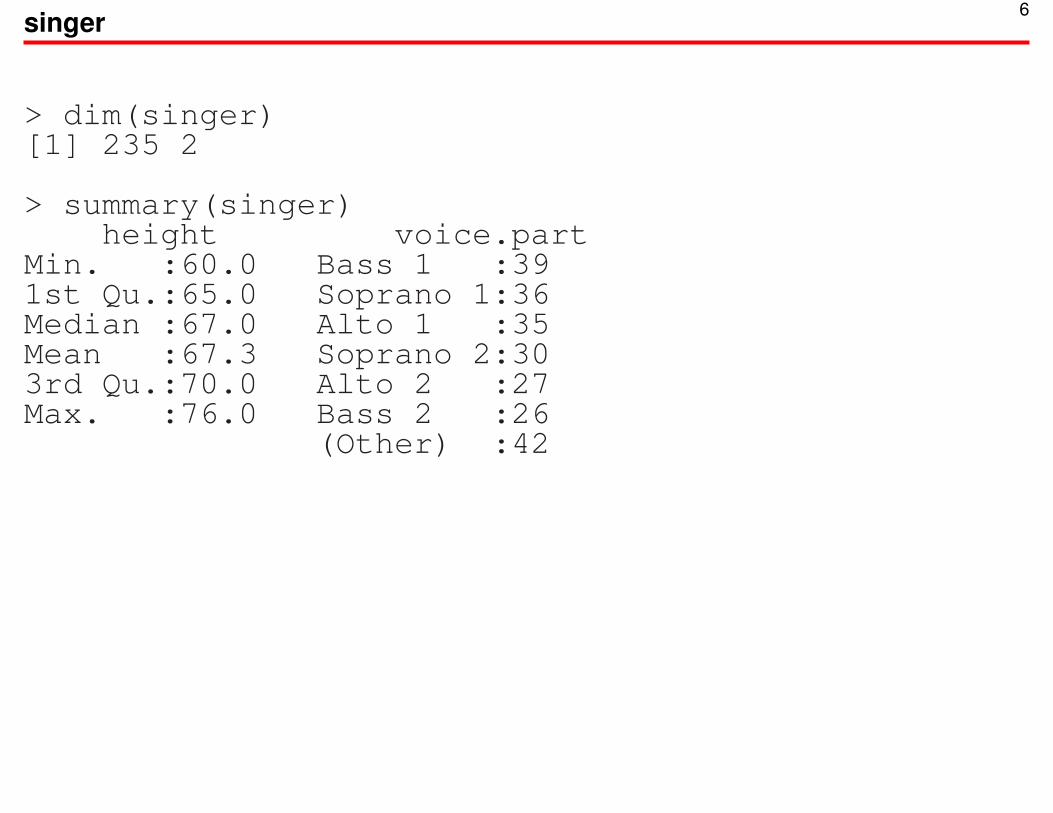
6singer

> dim(singer)[1] 235 2

> summary(singer)height voice.part

Min. :60.0 Bass 1 :391st Qu.:65.0 Soprano 1:36Median :67.0 Alto 1 :35Mean :67.3 Soprano 2:303rd Qu.:70.0 Alto 2 :27Max. :76.0 Bass 2 :26

(Other) :42

7bwplot()

bwplot(voice.part ˜ height,data = singer,aspect = 1,xlab = "Height (inches)")

8

Height (inches)

Bass 2

Bass 1

Tenor 2

Tenor 1

Alto 2

Alto 1

Soprano 2

Soprano 1

60 65 70 75

9stripplot()

stripplot(voice.part ˜ height,data = singer,aspect = 1,xlab = "Height (inches)",jitter = T)

10

Height (inches)

Bass 2

Bass 1

Tenor 2

Tenor 1

Alto 2

Alto 1

Soprano 2

Soprano 1

60 65 70 75

11qq()

qq(voice.part ˜ singer$height,data = singer,subset = voice.part=="Bass 2" | voice.part=="Tenor 1",aspect = 1,xlab = "Tenor 1 Height (inches)",ylab = "Base 2 Height (inches)"

)

12

Tenor 1 Height (inches)

Base 2

Heig

ht (inches)

64

66

68

70

72

74

76

64 66 68 70 72 74 76

13dotplot()

part.mean <- tapply(singer$height,singer$voice.part,mean)

dotplot(labels(part.mean) ˜ part.mean,aspect = 1,ylab = "Voice Part",xlab = "Mean Height (inches)")

14

Mean Height (inches)

Bass 2

Bass 1

Tenor 2

Tenor 1

Alto 2

Alto 1

Soprano 2

Soprano 1

64 66 68 70

15qqmath()

qqmath(˜height | voice.part,distribution = qunif,data = singer,panel = function(x, ...) {

panel.grid()panel.qqmath(x,...)

},layout = c(4,2),aspect = 1,xlab = "f-value",ylab = "Height (inches)")

16

f−value

Heig

ht (inches)

60

65

70

75

0.0 0.2 0.4 0.6 0.8 1.0

Bass 2 Bass 1

0.0 0.2 0.4 0.6 0.8 1.0

Tenor 2 Tenor 1

Alto 2

0.0 0.2 0.4 0.6 0.8 1.0

Alto 1 Soprano 2

0.0 0.2 0.4 0.6 0.8 1.0

60

65

70

75

Soprano 1

17histogram()

histogram(˜height | voice.part,data = singer,nint = 17,endpoints = c(59.5, 76.5),layout = c(4, 2),aspect = 1,xlab = "Height (inches)")

18

Height (inches)

Perc

ent of To

tal

0

10

20

30

40

60 65 70 75

Bass 2 Bass 1

60 65 70 75

Tenor 2 Tenor 1

Alto 2

60 65 70 75

Alto 1 Soprano 2

60 65 70 75

0

10

20

30

40

Soprano 1

19rubber

> dim(rubber)[1] 30 5

> summary(rubber)hardness tensile.strength abrasion.loss

Min. :45.00 Min. :119.0 Min. : 32.01st Qu.:60.25 1st Qu.:151.0 1st Qu.:113.2Median :71.00 Median :176.5 Median :165.0Mean :70.27 Mean :180.5 Mean :175.43rd Qu.:81.00 3rd Qu.:210.0 3rd Qu.:220.5Max. :89.00 Max. :237.0 Max. :372.0

ts.low ts.highMin. :-61.00 Min. : 0.01st Qu.:-29.00 1st Qu.: 0.0Median : -3.50 Median : 0.0Mean :-15.63 Mean :16.13rd Qu.: 0.00 3rd Qu.:30.0Max. : 0.00 Max. :57.0

20splom()

splom(˜rubber[,1:3],varnames = c("Hardness\n(degrees Shore)",

"Tensile Strength\n(kg/square cm)","Abrasion Loss\n(g/hp-hour)"))

21

Scatter Plot Matrix

Hardness

(degrees Shore)

70

80

9070 80 90

50

60

70

50 60 70

Tensile Strength

(kg/square cm)180

200

220

240180 200 220 240

120

140

160

180

120 140 160 180

Abrasion Loss

(g/hp−hour)200

250

300

350200 250 300 350

50

100

150

200

50 100 150 200

22contourplot()

attach(galaxy)galaxy.marginal <- list(east.west = seq(-25, 25,length=101),

north.south = seq(-45, 45,length=181))galaxy.grid <- expand.grid(galaxy.marginal)gal.m <- loess(velocity ˜ east.west * north.south,span = 0.25, degree = 2, normalize = F,family = "symmetric")galaxy.fit <- predict(gal.m, galaxy.grid)x <- range(galaxy.marginal$east.west)y <- range(galaxy.marginal$north.south)

contourplot(galaxy.fit ˜ galaxy.grid$east.west * galaxy.grid$north.south,

at = seq(1435, 1755, by = 10),aspect = diff(range(y))/diff(range(x)),xlab = "East-West Coordinate (arcsec)",ylab = "South-North Coordinate (arcsec)")

detach()

23

East−West Coordinate (arcsec)

So

uth

−No

rth

Co

ord

ina

te (

arc

se

c)

−40

−20

0

20

40

−20 −10 0 10 20

1435

1445

1455

146514751485149515051515

1515

15251535154515551565157515851595

160516151625

1635164516551665167516851695

17051715

17251735

1745

1755

24levelplot()

attach(soil)soi.grid <- expand.grid(

easting = seq(.15, 1.410, by = .015),northing = seq(.150, 3.645, by = .015))

soi.fit <- predict(loess(resistivity˜easting*northing,span = 0.25, degree = 2), soi.grid)

levelplot(soi.fit ˜ soi.grid$easting * soi.grid$northing,cuts = 9,colorkey = list(

labels = list(at = c(20, 40, 60, 80)),width = 5),

aspect=diff(range(soi.grid$n))/diff(range(soi.grid$e)),xlab = "Easting (km)",ylab = "Northing (km)")

detach()

25

Easting (km)

Nort

hin

g (

km

)

1

2

3

0.2 0.4 0.6 0.8 1.0 1.2

20

40

60

80

26wireframe()

attach(galaxy)galaxy.marginal <- list(east.west = seq(-25, 25, by = 2),

north.south = seq(-45, 45, by = 2))galaxy.grid <- expand.grid(galaxy.marginal)galaxy.fit <- predict(loess(velocity ˜ east.west*north.south,

span = 0.25, degree = 2, normalize = F,family = "symmetric"),

galaxy.grid)ar <- diff(range(galaxy.grid$north.south))/

diff(range(galaxy.grid$east.west))

wireframe(galaxy.fit ˜ galaxy.grid$east.west*galaxy.grid$north.south,screen = list(z = 30, x = -60, y = 0),aspect = c(ar, 1.3),xlab = "East-West",ylab = "South-North",zlab = "Velocity")

detach()

27

East−West

South−North

Velocity

28ethanol

> dim(ethanol)[1] 88 3

> summary(ethanol)NOx C E

Min. :0.370 Min. : 7.500 Min. :0.53501st Qu.:0.953 1st Qu.: 8.625 1st Qu.:0.7618Median :1.754 Median :12.000 Median :0.9320Mean :1.957 Mean :12.034 Mean :0.92653rd Qu.:3.003 3rd Qu.:15.000 3rd Qu.:1.1098Max. :4.028 Max. :18.000 Max. :1.2320

29Captions and Labels

Most general display functions allow four standard labels:

main, sub, xlab, ylab

Apart from their positions, they are treated identically

xyplot(NOx ˜ E,data = ethanol,aspect = 0.6,main = "Ethanol Data",sub = "Scatterplot of NOx vs E",xlab = "Equivalence Ratio",ylab = "NOx (micrograms/J)")

30

Ethanol Data

Scatterplot of NOx vs E

Equivalence Ratio

NOx (

mic

rogra

ms/J)

1

2

3

4

0.6 0.8 1.0 1.2

31Captions and Labels: Mathematical Expressions

xyplot(sqrt(NOx) ˜ Eˆ2,data = ethanol,aspect = 0.6,xlab = expression(Eˆ2),ylab = expression(sqrt(NOx)))

See ?plotmath for more mathematical expressions

32

E2

NO

x

1.0

1.5

2.0

0.5 1.0 1.5

33Captions and Labels: Other Graphical Parameters

xyplot(NOx ˜ E,data = ethanol,aspect = 0.6,xlab = list(

label = "Equivalence Ratio",col = "red",cex = 3,font = "italic"

),ylab = "NOx (micrograms/J)",)

See ?gpar for a full list

34

Equivalence Ratio

NOx (

mic

rogra

ms/J)

1

2

3

4

0.6 0.8 1.0 1.2

35

col Colour for lines and borders.

fill Colour for filling rectangles, polygons, ...

alpha Alpha channel for transparency

lty Line type

lwd: Line width

lex: Multiplier applied to line width

lineend: Line end style (round, butt, square)

linejoin: Line join style (round, mitre, bevel)

linemitre: Line mitre limit (number greater than 1)

36

fontsize: The size of text (in points)

cex: Multiplier applied to fontsize

fontfamily: The font family

fontface: The font face (bold, italic, ...)

lineheight: The height of a line as a multipleof the size of text

font: Font face (alias for fontface;for backward compatibility)

37Scales: dataset slope

> dim(slope)[1] 44 4

> slope[1:5, ]error percent distance resolution

1 18.90625 50 37.40523 5.0104592 16.33333 55 37.15230 4.5045903 19.43750 60 36.89979 3.9995974 17.44791 65 36.64780 3.4955495 17.03646 70 36.39627 2.992530

> summary(slope)error percent distance resolution

Min. : 3.104 Min. : 50 Min. : 0.265 Min. : 0.0001st Qu.: 6.262 1st Qu.: 60 1st Qu.: 9.875 1st Qu.: 1.952Median : 7.984 Median : 75 Median :21.368 Median : 4.493Mean : 9.362 Mean : 75 Mean :20.685 Mean : 5.8773rd Qu.:11.962 3rd Qu.: 90 3rd Qu.:31.281 3rd Qu.: 8.661Max. :19.438 Max. :100 Max. :37.405 Max. :19.470

38Scales: relation="same"

Default of relation is "same".

xyplot(error ˜ distance | as.factor(percent),data = slope,layout = c(6,2),xlab="Distance (degrees)",ylab="Absolute Error (%)")

or equivalently,

xyplot(error ˜ distance | as.factor(percent),data = slope,layout = c(6,2),scales = list(y="same"),xlab="Distance (degrees)",ylab="Absolute Error (%)")

or equivalently,

xyplot(error ˜ distance | as.factor(percent),data = slope,layout = c(6,2),scales = list(y=list(relation="same")),xlab="Distance (degrees)",ylab="Absolute Error (%)")

39

Distance (degrees)

Absolu

te E

rror

(%)

5

10

15

20

0 10 20 30

50 55

0 10 20 30

60 65

0 10 20 30

70 75

80

0 10 20 30

85 90

0 10 20 30

95

5

10

15

20

100

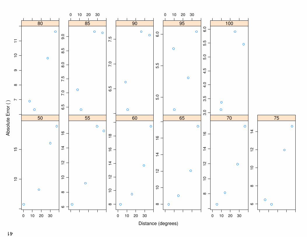
40Scales: relation="free"

xyplot(error ˜ distance | as.factor(percent),data = slope,layout = c(6,2),scales = list(y="free"),xlab="Distance (degrees)",ylab="Absolute Error (%)")

or equivalently,

xyplot(error ˜ distance | as.factor(percent),data = slope,layout = c(6,2),scales = list(y=list(relation="free")),xlab="Distance (degrees)",ylab="Absolute Error (%)")

41

Distance (degrees)

Absolu

te E

rror

(%)

10

15

0 10 20 30

50

68

10

12

14

16

55

810

12

14

16

18

0 10 20 30

60

810

12

14

16

65

810

12

14

16

0 10 20 30

70

68

10

12

14

75

78

910

11

80

0 10 20 30

6.5

7.0

7.5

8.0

8.5

9.0

85

6.5

7.0

7.5

90

0 10 20 30

5.0

5.5

6.0

95

3.0

3.5

4.0

4.5

5.0

5.5

6.0

100

42Scales: relation="sliced"

xyplot(error ˜ distance | as.factor(percent),data = slope,layout = c(6,2),scales = list(y="sliced"),xlab="Distance (degrees)",ylab="Absolute Error (%)")

or equivalently,

xyplot(error ˜ distance | as.factor(percent),data = slope,layout = c(6,2),scales = list(y=list(relation="sliced")),xlab="Distance (degrees)",ylab="Absolute Error (%)")

43

Distance (degrees)

Absolu

te E

rror

(%)

10

15

0 10 20 30

50

510

15

55

10

15

20

0 10 20 30

60

10

15

65

510

15

0 10 20 30

70

510

15

75

510

15

80

0 10 20 30

510

85

05

10

90

0 10 20 30

05

10

95

05

10

100

44Scales: tick.number

tick.number gives the ”suggested” number of intervals between ticks.

xyplot(error ˜ distance | as.factor(percent),data = slope,layout = c(6,2),scales = list(y=list(tick.number=8)),xlab="Distance (degrees)",ylab="Absolute Error (%)")

45

Distance (degrees)

Absolu

te E

rror

(%)

4

6

8

10

12

14

16

18

20

0 10 20 30

50 55

0 10 20 30

60 65

0 10 20 30

70 75

80

0 10 20 30

85 90

0 10 20 30

95

4

6

8

10

12

14

16

18

20

100

46Scales: at

at gives the location of tick marks along the axis.

xyplot(error ˜ distance | as.factor(percent),data = slope,layout = c(6,2),scales = list(

y=list(at=c(5,7.5,10,12.5,15,17.5,20))),xlab="Distance (degrees)",ylab="Absolute Error (%)")

47

Distance (degrees)

Absolu

te E

rror

(%)

5.0

7.5

10.0

12.5

15.0

17.5

20.0

0 10 20 30

50 55

0 10 20 30

60 65

0 10 20 30

70 75

80

0 10 20 30

85 90

0 10 20 30

95

5.0

7.5

10.0

12.5

15.0

17.5

20.0

100

48Scales: labels

labels gives vector of labels to go along with at.


y=list(at=c(5,10,15,20),labels=c("tick1","tick2","tick3","tick4"))

),xlab="Distance (degrees)",ylab="Absolute Error (%)")

49

Distance (degrees)

Absolu

te E

rror

(%)

tick1

tick2

tick3

tick4

0 10 20 30

50 55

0 10 20 30

60 65

0 10 20 30

70 75

80

0 10 20 30

85 90

0 10 20 30

95

tick1

tick2

tick3

tick4

100

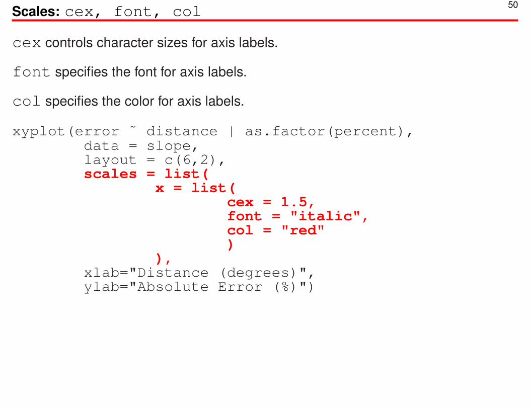
50Scales: cex, font, col

cex controls character sizes for axis labels.

font specifies the font for axis labels.

col specifies the color for axis labels.


x = list(cex = 1.5,font = "italic",col = "red")

),xlab="Distance (degrees)",ylab="Absolute Error (%)")

51

Distance (degrees)

Absolu

te E

rror

(%)

5

10

15

20

0 10 20 30

50 55

0 10 20 30

60 65

0 10 20 30

70 75

80

0 10 20 3085 90

0 10 20 3095

5

10

15

20

100

52Scales: alternating

alternating specifies whether axis labels should alternate from one side ofthe group of panels to the other.

xyplot(error ˜ distance | as.factor(percent),data = slope,layout = c(6,2),scales = list(x=list(alternating=FALSE)),xlab="Distance (degrees)",ylab="Absolute Error (%)")

53

Distance (degrees)

Absolu

te E

rror

(%)

5

10

15

20

0 10 20 30

50

0 10 20 30

55

0 10 20 30

60

0 10 20 30

65

0 10 20 30

70

0 10 20 30

75

80 85 90 95

5

10

15

20

100

54Scales: alternating

alternating can also be a vector (replicated to be as long as the number ofrows or columns per page) consisting of the following numbers

0: do not draw tick labels

1: bottom/left

2: top/right

3: both.

xyplot(error ˜ distance | as.factor(percent),data = slope,layout = c(6,2),scales = list(x=list(alternating=c(1,2)),

y=list(alternating=c(2,1))),xlab="Distance (degrees)",ylab="Absolute Error (%)")

55

Distance (degrees)

Absolu

te E

rror

(%)

0 10 20 30

50 55

0 10 20 30

60 65

0 10 20 30

70

5

10

15

20

75

5

10

15

20

80

0 10 20 30

85 90

0 10 20 30

95 100

56Scales

Without specifying x or y-axis, the arguments in scales are applied to both x andy-axis.

xyplot(error ˜ distance | as.factor(percent),data = slope,layout = c(6,2),scales = list(cex=1.5, col="red"),xlab="Distance (degrees)",ylab="Absolute Error (%)")

or equivalently,


x = list(cex=1.5, col="red"),y = list(cex=1.5, col="red"))

xlab="Distance (degrees)",ylab="Absolute Error (%)")

57

Distance (degrees)

Absolu

te E

rror

(%)

5

10

15

20

0 10 20 30

50 55

0 10 20 30

60 65

0 10 20 30

70 75

80

0 10 20 30

85 90

0 10 20 30

95

5

10

15

20100

58Scales: draw

draw specifies whether axis labels should be drawn.

xyplot(error ˜ distance | as.factor(percent),data = slope,layout = c(6,2),scales = list(y=list(draw=FALSE)),xlab="Distance (degrees)",ylab="Absolute Error (%)")

59

Distance (degrees)

Absolu

te E

rror

(%)

0 10 20 30

50 55

0 10 20 30

60 65

0 10 20 30

70 75

80

0 10 20 30

85 90

0 10 20 30

95 100

60Scales: limits

limits same as xlim and ylim, normally a numeric vector of length 2 giving leftand right limits for the axis.

xyplot(error ˜ distance | as.factor(percent),data = slope,layout = c(6,2),scales = list(y=list(limits=c(5,20))),xlab="Distance (degrees)",ylab="Absolute Error (%)")

61

Distance (degrees)

Absolu

te E

rror

(%)

10

15

0 10 20 30

50 55

0 10 20 30

60 65

0 10 20 30

70 75

80

0 10 20 30

85 90

0 10 20 30

95

10

15

100

62Scales: tck

tck a numeric scalar controlling the length of tick marks. Can also be a vector oflength 2, to control the length of left/bottom and right/top tick marks separately.

xyplot(error ˜ distance | as.factor(percent),data = slope,layout = c(6,2),scales = list(y=list(tck=c(2,1)),

x=list(tck=c(2,0.5))),xlab="Distance (degrees)",ylab="Absolute Error (%)")

63

Distance (degrees)

Absolu

te E

rror

(%)

5

10

15

20

0 10 20 30

50 55

0 10 20 30

60 65

0 10 20 30

70 75

80

0 10 20 30

85 90

0 10 20 30

95

5

10

15

20

100

64Scales: rot

rot Angle (in degrees) by which the axis labels are to be rotated. Can be a vectorof length 2, to control left/bottom and right/top axes separately.

xyplot(error ˜ distance | as.factor(percent),data = slope,layout = c(6,2),scales = list(y=list(rot=c(70, 10)),

x=list(rot=c(90, 20))),xlab="Distance (degrees)",ylab="Absolute Error (%)")

65

Distance (degrees)

Absolu

te E

rror

(%)

510

15

20

0

10

20

30

50 55

0

10

20

30

60 65

0

10

20

30

70 75

80

0 10 20 30

85 90

0 10 20 30

95

5

10

15

20

100

66Scales: abbreviate

abbreviate A logical flag, indicating whether to abbreviate the labels using theabbreviate function. Can be useful for long labels (e.g., in factors), especially on thex-axis.

slope$pc <- paste(slope$percent, "% percent", sep="")xyplot(error ˜ as.factor(pc),

data = slope,scales = list(x=list(abbreviate=TRUE,

minlength=5)),xlab="Distance (degrees)",ylab="Absolute Error (%)")

67

Distance (degrees)

Absolu

te E

rror

(%)

5

10

15

20

100%p 50%pr 55%pr 60%pr 65%pr 70%pr 75%pr 80%pr 85%pr 90%pr 95%pr

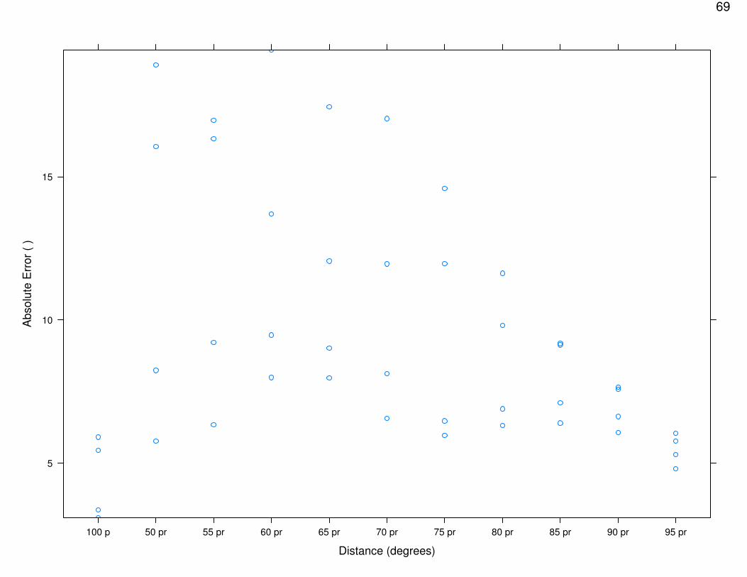
68Scales: axs

axsA character string, ”r” (default) or ”i”. In the latter case, the axis limits arecalculated as the exact data range, instead of being padded on either side.

slope$pc <- paste(slope$percent, "% percent", sep="")xyplot(error ˜ as.factor(pc),

data = slope,scales = list(x=list(abbreviate=TRUE,

minlength=5),y=list(axs="i")),

xlab="Distance (degrees)",ylab="Absolute Error (%)")

69

Distance (degrees)

Absolu

te E

rror

(%)

5

10

15

100%p 50%pr 55%pr 60%pr 65%pr 70%pr 75%pr 80%pr 85%pr 90%pr 95%pr

70Key: auto.key

xyplot(error ˜ distance,groups = as.factor(percent),data = subset(slope, percent <= 70),auto.key = TRUE,type = "b",scales = list(y=list(tick.number=8)),xlab="Distance (degrees)",ylab="Absolute Error (%)"

)

71

Distance (degrees)

Absolu

te E

rror

(%)

6

8

10

12

14

16

18

20

0 10 20 30

5055606570

72Key: points

label <- levels(as.factor(subset(slope, percent <=70)$percent)

)xyplot(error ˜ distance,

groups = as.factor(percent),data = subset(slope, percent <= 70),auto.key = TRUE,type = "p",pch = 1:5,col = 1:5,key = list(type = c("p"),

text = list(label = label, cex = 1.2),points = list(col=1:5, pch = 1:5),column = 5,space = "top"),

scales = list(y=list(tick.number=8)),xlab="Distance (degrees)",ylab="Absolute Error (%)")

73

Distance (degrees)

Absolu

te E

rror

(%)

6

8

10

12

14

16

18

20

0 10 20 30

50 55 60 65 70

74Key: lines

xyplot(error ˜ distance,groups = as.factor(percent),data = subset(slope, percent <= 70),auto.key = TRUE,type = "l",lty = 1:5,lwd = 1.5,col = 1:5,key = list(type = "l",

text = list(label = label),lines = list(col=1:5, lty=1:5, lwd=1.5),column = 5,space = "top"),


75

Distance (degrees)

Absolu

te E

rror

(%)

6

8

10

12

14

16

18

20

0 10 20 30

50 55 60 65 70

76Key: both

xyplot(error ˜ distance,groups = as.factor(percent),data = subset(slope, percent <= 70),auto.key = TRUE,type = "b",pch = 1:5,col = 1:5,key = list(type = c("l"),

text = list(label = label),lines = list(col =1:5, lwd =1.5),points = list(col=1:5, pch = 1:5),column = 5,space = "top"),


77

Distance (degrees)

Absolu

te E

rror

(%)

6

8

10

12

14

16

18

20

0 10 20 30

50 55 60 65 70

78Type: distribute.type

xyplot(error ˜ distance,groups = as.factor(percent),data = subset(slope, percent < 60),type = c("b","l"),distribute.type = TRUE,pch = 16,col = 1:2,lwd = 1.5,cex = 2,scales = list(y=list(tick.number=8)),xlab="Distance (degrees)",ylab="Absolute Error (%)")

79

Distance (degrees)

Absolu

te E

rror

(%)

6

8

10

12

14

16

18

0 10 20 30

80Strip

xyplot(error ˜ distance | as.factor(percent),data = slope,strip = strip.custom(

par.strip.text= list(cex = 1.5, col = "red")),

par.settings = list(layout.heights = list(strip = 1.5),strip.background=list(col="lightgrey")),


81

Distance (degrees)

Absolu

te E

rror

(%)

4

6

8

10

12

14

16

18

20

0 10 20 30

50 55

0 10 20 30

60 65

70 75 80

4

6

8

10

12

14

16

18

20

85

4

6

8

10

12

14

16

18

20

90

0 10 20 30

95 100

82Strip: strip.left

xyplot(error ˜ distance | as.factor(percent),data = slope,strip = FALSE,strip.left =

strip.custom(par.strip.text=list(cex = 1.5, col = "red")),

par.settings = list(layout.heights = list(strip = 1.5),strip.background=list(col="lightgrey")),


83

Distance (degrees)

Absolu

te E

rror

(%)

4

6

8

10

12

14

16

18

20

0 10 20 30

50

55

0 10 20 30

60

65

70

75

80

4

6

8

10

12

14

16

18

20

85

4

6

8

10

12

14

16

18

2090

0 10 20 30

95

100

84Panel Function: panel.points

xyplot(error ˜ distance | percent,data = slope,pch = 16,panel = function(x,y,...){

panel.xyplot(x,y,...)panel.points(mean(x), mean(y), col="red")

})

85

distance

err

or

5

10

15

20

0 10 20 30

percent percent

0 10 20 30

percent percent

percent percent percent

5

10

15

20percent

5

10

15

20percent

0 10 20 30

percent percent

86Panel Function: panel.mathdensity

histogram( ˜ height | voice.part,data = singer,nint = 17,type = "density",endpoints = c(59.5, 76.5),layout = c(4, 2),aspect = 1,xlab = "Height (inches)",panel = function(x,...){

panel.histogram(x,...)panel.mathdensity(dmath = dnorm,

col = "red",lwd = 1,args = list(

mean=mean(x),sd=sd(x)), ...)

})

87

Height (inches)

Density

0.0

0.1

0.2

0.3

0.4

60 65 70 75

Bass 2 Bass 1

60 65 70 75

Tenor 2 Tenor 1

Alto 2

60 65 70 75

Alto 1 Soprano 2

60 65 70 75

0.0

0.1

0.2

0.3

0.4

Soprano 1

88Panel Function: panel.arrows

xyplot(error ˜ distance,data=slope,panel=function(x,y,...){

panel.xyplot(x,y,...)for(i in 1:(length(x)-1)){

panel.arrows(x[i],y[i],x[i+1],y[i+1],angle=10, code=2, length=0.2,...)

}}

)

89

distance

err

or

5

10

15

20

0 10 20 30

90Panel Function: panel.abline

xyplot(error ˜ distance | percent,data = slope,panel = function(x,y,...){

panel.abline(h=mean(y), v=mean(x),lty=3,...)

panel.xyplot(x,y,...)}

)

91

distance

err

or

5

10

15

20

0 10 20 30

percent percent

0 10 20 30

percent percent


5

10

15

20percent

5

10

15

20percent

0 10 20 30

percent percent



cof <- lm(y ˜ x)$coefficientspanel.abline(a=cof[1], b=cof[2],

col="red", ...)panel.xyplot(x,y,...)

})

or equivalently,


cof <- lm(y ˜ x)panel.abline(reg = cof, col="red", ...)panel.xyplot(x,y,...)

})


or equivalently,


cof <- lm(y ˜ x)panel.lmline(x,y,col="red", ...)panel.xyplot(x,y,...)

})

94

distance

err

or

5

10

15

20

0 10 20 30

percent percent

0 10 20 30

percent percent


5

10

15

20percent

5

10

15

20percent

0 10 20 30

percent percent

95Panel Function: panel.refline

or equivalently,


cof <- lm(y ˜ x)panel.refline(v=mean(x), h=mean(y),...)panel.xyplot(x,y,...)

})

96

distance

err

or

5

10

15

20

0 10 20 30

percent percent

0 10 20 30

percent percent


5

10

15

20percent

5

10

15

20percent

0 10 20 30

percent percent

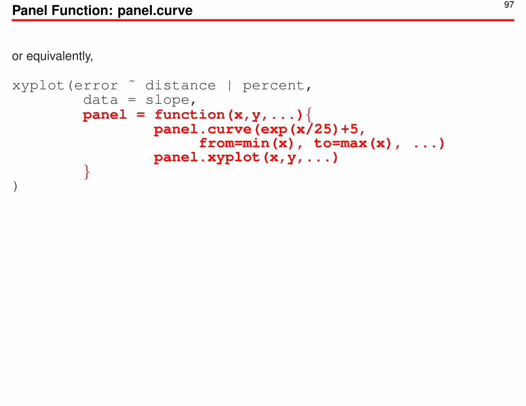
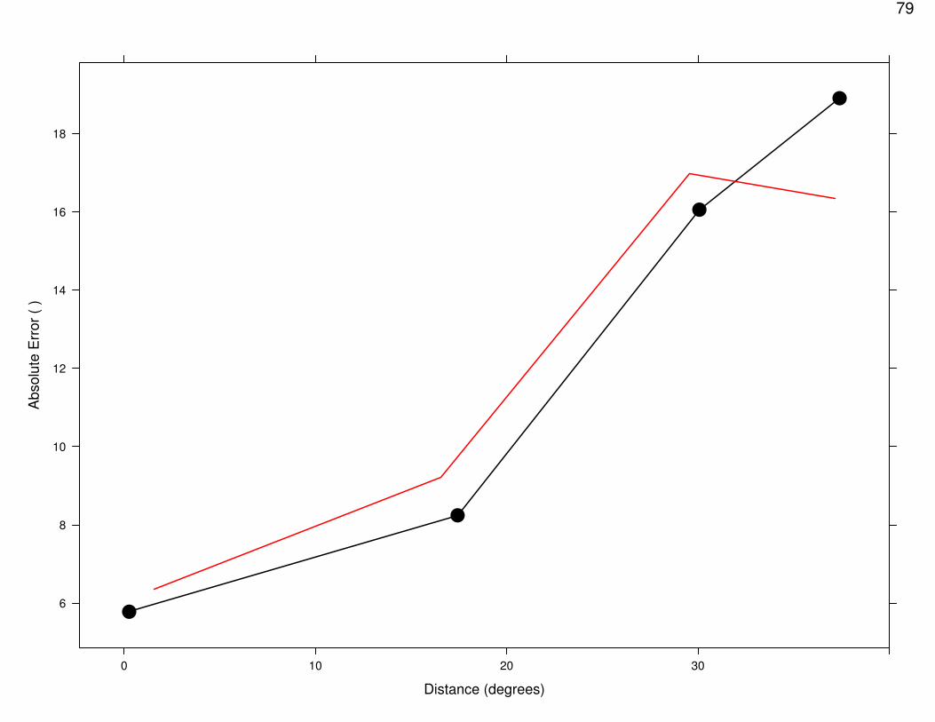
97Panel Function: panel.curve

or equivalently,


panel.curve(exp(x/25)+5,from=min(x), to=max(x), ...)


)

98

distance

err

or

5

10

15

20

0 10 20 30

99Panel Function: panel.grid

xyplot(error ˜ distance,data = slope,panel = function(x,y,...){

panel.grid(h=-1, v=-1, col="red", ...)panel.xyplot(x,y,...)

})

100

distance

err

or

5

10

15

20

0 10 20 30

101Panel Function: panel.average

xyplot(error ˜ percent,data = slope,panel = function(x,y,...){

panel.xyplot(x,y,...)panel.grid(h=-1, v=-1,col="black",

lty=3,...)panel.average(x,y,fun = mean,

horizontal = FALSE,col="black",...)

})

or equivalently,

xyplot(error ˜ percent,data = slope,panel = function(x,y,...){

panel.xyplot(x,y,...)panel.grid(h=-1, v=-1,col="black",

lty=3,...)panel.linejoin(x, y, fun = mean,

horizontal = FALSE,col="black", ...)

})

102

percent

err

or

5

10

15

20

50 60 70 80 90 100

103Panel Function: panel.segments


panel.segments( min(x), y[which.min(x)],min(x), 0, col="red", ...)


)

104

distance

err

or

5

10

15

20

0 10 20 30

percent percent

0 10 20 30

percent percent


5

10

15

20percent

5

10

15

20percent

0 10 20 30

percent percent

105Panel Function: panel.segments


panel.segments(rep(min(x),2), rep(y[which.min(x)],2),c(0, min(x)), c(y[which.min(x)], 0),col="red", ...)


)

106

distance

err

or

5

10

15

20

0 10 20 30

percent percent

0 10 20 30

percent percent


5

10

15

20percent

5

10

15

20percent

0 10 20 30

percent percent

107Panel Function: panel.text


panel.segments(rep(min(x),2), rep(y[which.min(x)],2),c(0, min(x)), c(y[which.min(x)], 0),col="red", ...)

panel.text(min(x), y[which.min(x)],round(min(x),2), adj=c(0,0))


)

108

distance

err

or

5

10

15

20

0 10 20 30

0.26

percent

1.57

percent

0 10 20 30

2.8

percent

3.94

percent

5

percent

5.98

percent

6.9

percent

5

10

15

20

7.76

percent

5

10

15

20

8.56

percent

0 10 20 30

9.3

percent

9.5

percent

109Aspect Ratio: aspect

number controls the ratio of physical height to physical length.

"fill" default, tries to make the panels as big as possible to fill the availablespace.

"xy" computes the aspect ratio based on the 45 degree banking rule.

"iso" forces relation between physical distance and distance in the data scale arethe same for both axes.

xyplot(error ˜ resolution,data=slope,aspect = "fill",

)

110

resolution

err

or

5

10

15

20

0 5 10 15 20

111Aspect: ”xy”

xyplot(error ˜ resolution,data=slope,aspect = "xy",

)

112

resolution

err

or

5101520

0 5 10 15 20

113Aspect: ”iso”

xyplot(error ˜ resolution,data=slope,aspect = "iso",

)

114

resolution

err

or

5

10

15

20

0 5 10 15 20

115Prepanel: Prepanel.default

Prepanel A function that takes the same arguments as the panel function andreturns a list, containing components named xlim, ylim, dx, and dy.

Every lattice graphic function has a default prepanel function named as:

prepanel.default.functionname

116Prepanel: prepandel.default.xyplot

xyplot(error ˜ resolution,data=slope,aspect = "xy",prepanel = function(x,y,...){

prepanel.default.xyplot(x,y,...)},panel = function(x,y,...){

panel.xyplot(x,y,...)panel.loess(x,y,span=2/3, degree=2,

col="red", ...)}

)

117

resolution

err

or

5101520

0 5 10 15 20



a <- prepanel.default.xyplot(x,y,...)print(a)

},panel = function(x,y,...){


col="red", ...)}

)


$xlim[1] 0.00000 19.47035

$ylim[1] 3.104167 19.437500

$dx[1] 0.0000000 0.0000000 0.0000000 0.4953526 0.4189504[6] 0.0778560 0.3851590 0.0151460 0.0978860 0.3482900

[11] 0.1512160 0.5007510 0.2820770 0.0283220 0.0822070[16] 0.1093170 0.5030190 0.2205400 0.2835080 0.2720060[21] 0.2091870 0.0238000 0.1638890 0.3419800 0.6189900[26] 0.1599810 0.4049100 0.4042260 0.7559930 0.2208100[31] 0.4581610 0.5258490 0.4074310 0.5832790 0.4583910[36] 0.6171700 1.5039100 0.2006800 1.7491200 0.3277300[41] 1.4643000 0.9796300 2.6193300


$dy[1] 0.458336 -2.812499 0.265623 2.671876[5] -0.734376 2.276040 -2.781250 0.968750[9] 3.364590 -1.479170 3.973960 2.968750

[13] 5.416669 -3.104166 0.557295 10.401040[17] 0.411450 -7.630200 9.619790 -13.031250[21] 0.708330 9.218750 -4.359370 6.932290[25] -6.947920 -5.635414 0.578124 5.156250[29] -6.088540 7.729170 -7.218754 10.494794[33] -8.838540 7.921860 -9.484360 2.453121[37] -1.052081 1.505210 -0.265629 -1.218751[41] 0.250001 -1.895831 -0.567710

$xatNULL

$yatNULL


vihi

=vi

hi

· (v/v

h/h) =

v

h· (

vi/v

hi/h)

vi: length of vertical side in physical unit for i’th segment

hi: length of horizontal side in physical unit for i’th segment

vi: length of vertical side in data unit for i’th segment

hi: length of horizontal side in data unit for i’th segment

v: length of vertical side in physical unit for whole data

h: length of horizontal side in physical unit for whole data

v: length of vertical side in data unit for whole data

h: length of horizontal side in data unit for whole data



a <- prepanel.default.xyplot(x,y,...)ydif <- diff(a$ylim)xdif <- diff(a$xlim)b <- abs((a$dy/a$dx)/(ydif/xdif))print(1/median(b))



col="red", ...)}

)

[1] 0.05324232

123Prepanel: prepandel.default.qqmath

qqmath(˜ error,data=slope,aspect = "xy",prepanel = function(x,...){

a <- prepanel.default.qqmath(x,...)print(a)

},panel = function(x,...){

panel.qqmathline(x,...)panel.qqmath(x,...)

})

124

qnorm

err

or

5

10

15

20

−2 −1 0 1 2

125Prepanel: prepandel.default.qqmath


a <- prepanel.default.qqmath(x,...)print(a)ydif <- diff(a$ylim)xdif <- diff(a$xlim)b <- abs((a$dy/a$dx)/(ydif/xdif))print(1/median(b))



})

[1] 1.879839

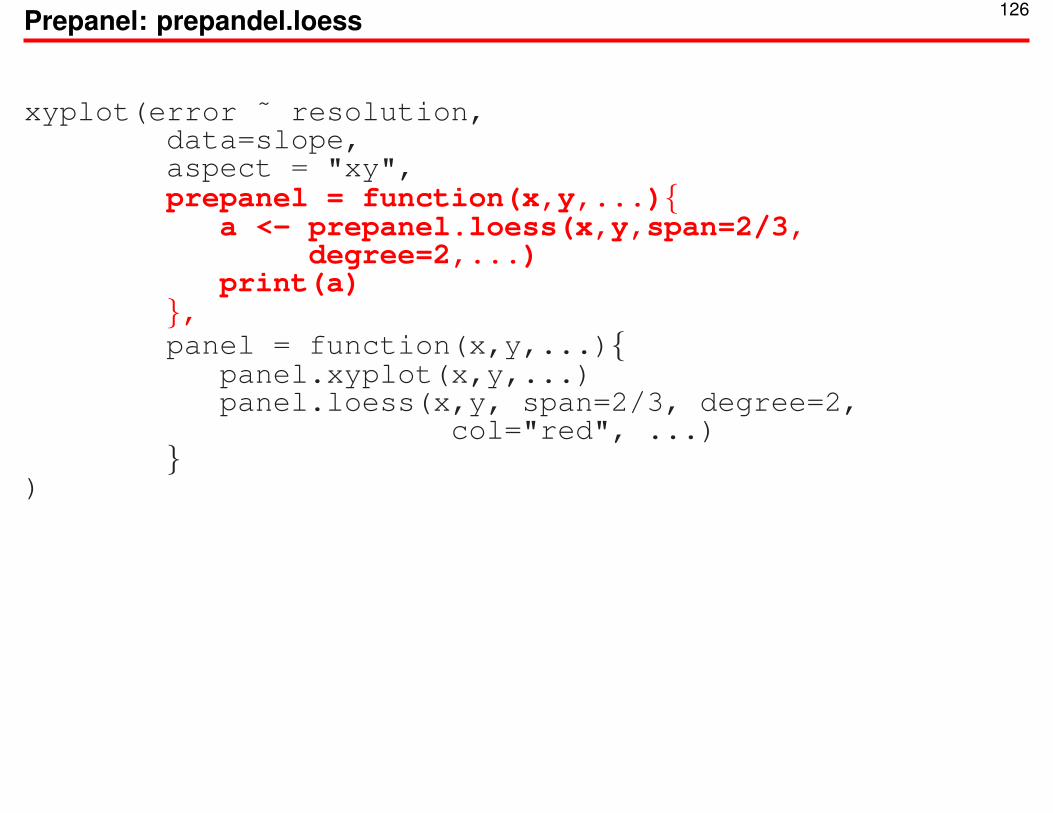
126Prepanel: prepandel.loess


a <- prepanel.loess(x,y,span=2/3,degree=2,...)

print(a)},panel = function(x,y,...){

panel.xyplot(x,y,...)panel.loess(x,y, span=2/3, degree=2,

col="red", ...)}

)

127

resolution

err

or

5

10

15

20

0 5 10 15 20

128Prepanel: prepandel.loess


a <- prepanel.loess(x,y,span=2/3,degree=2,...)

ydif <- diff(a$ylim)xdif <- diff(a$xlim)b <- abs((a$dy/a$dx)/(ydif/xdif))print(1/median(b))


panel.xyplot(x,y,...)panel.loess(x,y,span=2/3,

degree=2, col="red", ...)}

)

[1] 1.818469

129Prepanel: prepandel.qqmathline


a <- prepanel.qqmathline(x,...)print(a)



})

$xlim[1] -2.277988 2.277988$ylim[1] 3.104167 19.437500$dx[1] 1.34898$dy[1] 5.700519

130

qnorm

err

or

5

10

15

20

−2 −1 0 1 2

131Custom prepanel function

prepanel <- function(x,...){ans <- prepanel.qqmathline(x,...)theo.quant <- qnorm(c(.25,.75))data.quant <- quantile(x, c(.25,.75), names = F)slope <- ans$dy / ans$dxintercept <- data.quant[1] - slope*theo.quant[1]yylim <- slope*(ans$xlim)+ interceptans$ylim <- range(ans$ylim, yylim)ans

}qqmath(˜ error,

data=slope,aspect = "xy",prepanel = function(x,...){

prepanel(x)},

panel = function(x,...){panel.qqmathline(x,...)panel.qqmath(x,...)

})

132

qnorm

err

or

0

5

10

15

20

−2 −1 0 1 2

> attach(h:/lattice.rdata) - purdue...

Documents