atomis’c)materials)simula’on)using)quantum5...

Sandia National Laboratories is a multi-program laboratory managed and operated by Sandia Corporation, a wholly owned subsidiary of Lockheed Martin Corporation, for the U.S. Department of Energy’s National Nuclear Security Administration under contract DE-AC04-94AL85000. SAND NO. 2013-XXXXP

Atomis'c Materials Simula'on Using Quantum-‐Accurate Interatomic Poten'als

Aidan Thompson Compu'ng Research Center

Sandia Na'onal Laboratories, New Mexico IPAM, February 25, 2015, SAND 2014-‐1297C

What is Molecular Dynamics Simula'on?

2

Distance

Tim

e

Å m

10-1

5 s

year

s

QM MD

MESO

Design

MD Engine !

HNS atoms, positions, velocities

interatomic potential Positions, velocities and forces at many later times!

•  Continuum models require underlying models of the materials behavior

•  Quantum methods can provide very complete description for 100s of atoms

•  Molecular Dynamics acts as the “missing link” •  Bridges between quantum and continuum

models •  Moreover, extends quantum accuracy to

continuum length scales; retaining atomistic information

Example: Plas'city in BCC Metals

3

Screw Dislocation Motion in BCC Tantalum VASP DFT

N≈100

Weinberger, Tucker, and Foiles, PRB (2013)

LAMMPS MD N≈108

Polycrystalline Tantalum Sample

(Large-scale Atomic/Molecular Massively Parallel Simulator)

http://lammps.sandia.gov

•  Classical MD code. •  Open source, highly portable C++. •  Freely available for download under GPL. •  Easy to download, install, and run. •  Well documented. •  Easy to modify or extend with new features and func'onality. •  Ac've user’s e-‐mail list with over 650 subscribers. •  More that 1000 cita'ons/year •  Users’ workshops: 2010, 2011, 2013, 2015 •  Spa'al-‐decomposi'on of simula'on domain for parallelism. •  Energy minimiza'on via conjugate-‐gradient relaxa'on. •  Atomis'c, mesoscale, and coarse-‐grain simula'ons. •  Variety of poten'als (including many-‐body and coarse-‐grain). •  Variety of boundary condi'ons, constraints, etc.

What is LAMMPS?

2012 Top Application Codes at NERSC

MD is Big Consumer of Computer Time

Climate

QCD Physics

QCD Physics

Plasma Physics

5

DFT

LAMMPS

NAMD

GROMACS

Exponen'al Growth in Use of MD

6

Papers citing LAMMPS, NAMD, GROMACS Measured using Web of Science citation reports

2000 2005 2010 2015Year

0.1

1

10ki

lopa

pers

/yea

rTop 3 MD Codes

1.5 years

3 years

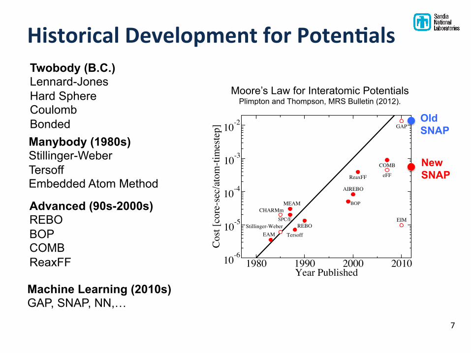
Historical Development for Poten'als

Moore’s Law for Interatomic Potentials Plimpton and Thompson, MRS Bulletin (2012).

Moore’s Law for potentials

CHARMm

EAMStillinger-Weber

Tersoff

AIREBO

MEAM

ReaxFF eFF

COMB

EIM

BOP

GAP

REBOSPC/E

1980 1990 2000 2010Year Published

10-6

10-5

10-4

10-3

10-2

Cost

[cor

e-se

c/at

om-ti

mes

tep]

Old SNAP

New SNAP

7

Twobody (B.C.) Lennard-Jones Hard Sphere Coulomb Bonded Manybody (1980s) Stillinger-Weber Tersoff Embedded Atom Method

Advanced (90s-2000s) REBO BOP COMB ReaxFF

Machine Learning (2010s) GAP, SNAP, NN,…

Two philosophical extremes in the development of interatomic potential models

•  Functional forms based on fundamental understanding of electronic origins of bonding

•  Bond Order Potentials (BOP) •  Model Generalized Pseudopotential

Theory (MGPT) •  COMB •  ReaxFF •  …

•  Gives confidence that it will interpolate/extrapolate reasonably

•  Empirical fit of a flexible functional form

•  Gaussian Approximation Potentials (GAP)

•  Spectral Neighbor Analysis Potential (SNAP) - this work

•  … •  Replaces the need for intuition/art

with extensive computation •  Automate the fitting process? •  Apply across multiple materials classes?

Luke: Is the dark side stronger? Yoda: No, no no. Quicker, easier, more seductive.

The Force!

Darth Vader: You underestimate the power of the dark side!

The Dark Side!

Borrowed from Stephen Foiles 8

SNAP: Spectral Neighbor Analysis Potentials

•  GAP (Gaussian Approximation Potential): Bartok, Csanyi et al., Phys. Rev. Lett, 2010. Uses 3D neighbor density bispectrum and Gaussian process regression.

•  SNAP (Spectral Neighbor Analysis Potential): Our SNAP approach uses GAP’s neighbor bispectrum, but replaces Gaussian process with linear regression. -  More robust -  Lower computational cost -  Decouples MD speed from training set size -  Enables large training data sets, more bispectrum coefficients -  Straightforward sensitivity analysis

ESNAP = EiSNAP

i=1

N

∑ + φijrep rij( )

j<i

N

∑

EiSNAP = β0 + βkB

ik

k∈ J<Jmax{ }∑

Geometric descriptors of atomic

environments

Energy as a function of geometric descriptors

9

Bispectrum Components as Descriptor •  Neighbors of each atom are mapped onto unit sphere in 4D

•  Expand density around each atom in a basis of 4D hyperspherical harmonics,

•  Bispectrum components of the 4D hyperspherical harmonic expansion are used as the geometric descriptors of the local environment

•  Preserves universal physical symmetries •  Rotation, translation, permutation •  Size-consistent

θ0,θ,φ( ) = θ0max r rcut , cos

−1(z r), tan−1(y x)( )

It is advantageous to use most of the 3-sphere, while still excluding theregion near the south pole where the configurational space becomes highlycompressed.

The natural basis for functions on the 3-sphere is formed by the 4D hy-perspherical harmonics U j

m,m

0(✓0, ✓,�), defined for j = 0, 12 , 1, . . . and m,m0 =�j,�j+1, . . . , j�1, j [9]. These functions also happen to be the elements ofthe unitary transformation matrices for spherical harmonics under rotationby angle 2✓0 about the axis defined by (✓,�). When the rotation is parame-terized in terms of the three Euler angles, these functions are better knownas Dj

m,m

0(↵, �, �), the Wigner D-functions, which form the representations ofthe SO(3) rotational group [10, 9]. Dropping the atom index i, the neighbordensity function can be expanded in the U j

m,m

0 functions

⇢(r) =1X

j=0, 12 ,...

jX

m=�j

jX

m

0=�j

uj

m,m

0Uj

m,m

0(✓0, ✓,�) (3)

where the expansion coe�cients are given by the inner product of theneighbor density with the basis function. Because the neighbor density is aweighted sum of �-functions, each expansion coe�cient can be written as asum over discrete values of the corresponding basis function,

uj

m,m

0 = U j

m,m

0(0, 0, 0) +X

rii0<Rcut

fc

(rii

0)wi

U j

m,m

0(✓0, ✓,�) (4)

The expansion coe�cients uj

m,m

0 are complex-valued and they are notdirectly useful as descriptors, because they are not invariant under rotationof the polar coordinate frame. However, the following scalar triple productsof expansion coe�cients can be shown to be real-valued and invariant underrotation [7].

Bj1,j2,j =

j1X

m1,m01=�j1

j2X

m2,m02=�j2

jX

m,m

0=�j

(uj

m,m

0)⇤Hjmm0

j1m1m01

j2m2m02

uj1

m1,m01uj2

m2,m02

(5)

The constantsHjmm0

j1m1m01

j2m2m02

are coupling coe�cients, analogous to the Clebsch-

Gordan coe�cients for rotations on the 2-sphere. These invariants are thecomponents of the bispectrum. They characterize the strength of densitycorrelations at three points on the 3-sphere. The lowest-order components

5

It is advantageous to use most of the 3-sphere, while still excluding theregion near the south pole where the configurational space becomes highlycompressed.

The natural basis for functions on the 3-sphere is formed by the 4D hy-perspherical harmonics U j

m,m

0(✓0, ✓,�), defined for j = 0, 12 , 1, . . . and m,m0 =�j,�j+1, . . . , j�1, j [9]. These functions also happen to be the elements ofthe unitary transformation matrices for spherical harmonics under rotationby angle 2✓0 about the axis defined by (✓,�). When the rotation is parame-terized in terms of the three Euler angles, these functions are better knownas Dj

m,m

0(↵, �, �), the Wigner D-functions, which form the representations ofthe SO(3) rotational group [10, 9]. Dropping the atom index i, the neighbordensity function can be expanded in the U j

m,m

0 functions

⇢(r) =1X

j=0, 12 ,...

jX

m=�j

jX

m

0=�j

uj

m,m

0Uj

m,m

0(✓0, ✓,�) (3)

where the expansion coe�cients are given by the inner product of theneighbor density with the basis function. Because the neighbor density is aweighted sum of �-functions, each expansion coe�cient can be written as asum over discrete values of the corresponding basis function,

uj

m,m

0 = U j

m,m

0(0, 0, 0) +X

rii0<Rcut

fc

(rii

0)wi

U j

m,m

0(✓0, ✓,�) (4)

The expansion coe�cients uj

m,m

0 are complex-valued and they are notdirectly useful as descriptors, because they are not invariant under rotationof the polar coordinate frame. However, the following scalar triple productsof expansion coe�cients can be shown to be real-valued and invariant underrotation [7].

Bj1,j2,j =

j1X

m1,m01=�j1

j2X

m2,m02=�j2

jX

m,m

0=�j

(uj

m,m

0)⇤Hjmm0

j1m1m01

j2m2m02

uj1

m1,m01uj2

m2,m02

(5)

The constantsHjmm0

j1m1m01

j2m2m02

are coupling coe�cients, analogous to the Clebsch-

Gordan coe�cients for rotations on the 2-sphere. These invariants are thecomponents of the bispectrum. They characterize the strength of densitycorrelations at three points on the 3-sphere. The lowest-order components

5

describe the coarsest features of the density function, while higher-order com-ponents reflect finer detail. An analogous bispectrum can be defined onthe 2-sphere in terms of the spherical harmonics. In this case, the compo-nents of the bispectrum are a superset of the second and third order bond-orientational order parameters developed by Steinhardt et al. [11]. These inturn are specific instances of the order parameters introduced in Landau’stheory of phase transitions [12].

The coupling coe�cients are non-zero only for non-negative integer andhalf-integer values of j1, j2, and j satisfying the conditions kj1�j2k j j1+j2 and j1+ j2� j not half-integer [10]. In addition, B

j1,j2,j is symmetric in j1and j2. Hence the number of distinct non-zero bispectrum components withindices j1, j2, j not exceeding a positive integer J is (J +1)3. Furthermore, itis proven in the appendix that bispectrum components with reordered indicesare related by the following identity:

Bj1,j2,j

2j + 1=

Bj,j2,j1

2j1 + 1=

Bj1,j,j2

2j2 + 1. (6)

We can exploit this equivalence by further restricting j2 j1 j, inwhich case the number of distinct bispectrum components drops to (J +1)(J + 2)(J + 3

2)/3, a three-fold reduction in the limit of large J .

2.2. SNAP Potential Energy Function

Given the bispectrum components as descriptors of the neighborhood ofeach atom, it remains to express the potential energy of a configuration ofN atoms in terms of these descriptors. We write the energy of the systemcontaining N atoms with positions rN as the sum of a reference energy E

ref

and a local energy Elocal

E(rN) = Eref

(rN) + Elocal

(rN). (7)

The reference energy includes known physical phenomena, such as long-range electrostatic interactions, for which well-established energy models ex-ist. E

local

must capture all the additional e↵ects that are not accounted forby the reference energy. Following Bartok et al. [1, 7] we assume that thelocal energy can be decomposed into separate contributions for each atom,

Elocal

(rN) =NX

i=1

Ei

(qi

) (8)

6

Symmetry relation: 10

SNAP FiKng Process FitSnap.py

11

Dakota optimization,

sensitivity

“Hyper-parameters” •  Cutoff distance •  Group Weights •  Number of Terms •  Etc.

fitsnap.py Communicate with

LAMMPS; weighted regression to obtain SNAP coefficients

LAMMPS

QUEST QDFT

Training Data

Metrics •  Force residuals •  Energy residuals •  Elastic constants •  Etc.

Bispectrum components & derivatives, reference potential

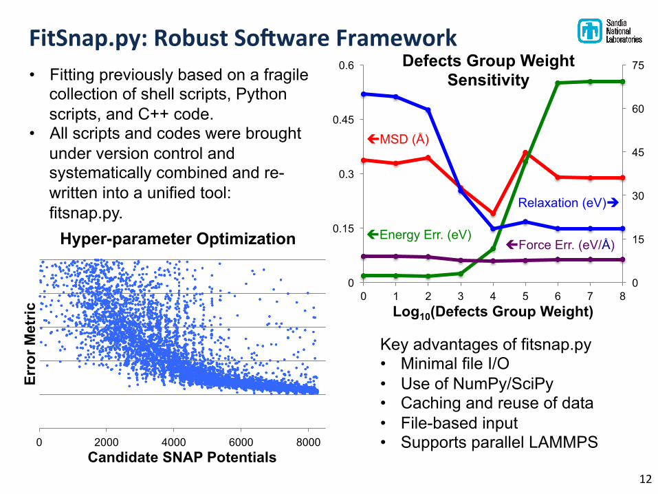
FitSnap.py: Robust SoPware Framework

12

•  Fitting previously based on a fragile collection of shell scripts, Python scripts, and C++ code.

•  All scripts and codes were brought under version control and systematically combined and re-written into a unified tool: fitsnap.py.

Key advantages of fitsnap.py •  Minimal file I/O •  Use of NumPy/SciPy •  Caching and reuse of data •  File-based input •  Supports parallel LAMMPS 0 2000 4000 6000 8000

Erro

r Met

ric

Candidate SNAP Potentials

Hyper-parameter Optimization

0

15

30

45

60

75

0

0.15

0.3

0.45

0.6

0 1 2 3 4 5 6 7 8

Log10(Defects Group Weight)

Defects Group Weight Sensitivity

Relaxation (eV)è

çForce Err. (eV/Å)

çMSD (Å)

çEnergy Err. (eV)

Ta SNAP potential was fit to a DFT-based training set containing ‘usual suspects’

For each configuration in training set, fit total energy, atomic forces, stress •  Equilibrium lattice parameter •  Elastic constants (C11, C12, and C44) and bulk modulus (B) •  Free surface energies: (100), (110), (111), and (112) •  Generalized planar stacking fault curves: {112} and {110} •  Energy-Volume (Contraction and Dilation) - BCC, FCC, HCP, and A15 •  Lattices with random atomic displacements •  Liquid structure

Example: DFT-based Generalized Stacking Fault Energies (112) (110)

13

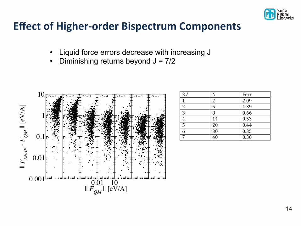
Effect of Higher-‐order Bispectrum Components

2J" N" Ferr"1" 2" 2.09"2" 5" 1.39"3" 8" 0.66"4" 14" 0.53"5" 20" 0.44"6" 30" 0.35"7" 40" 0.30""

•  Liquid force errors decrease with increasing J •  Diminishing returns beyond J = 7/2

0.001

0.01

0.1

1

10

|| FSN

AP -

F QM

|| [e

V/A

]

2J = 1 2J = 2 2J = 3

0.01 10|| FQM || [eV/A]

2J = 4 2J = 5 2J = 6 2J = 7

14

SNAP poten'al yields good agreement with DFT results for some standard proper'es

DFT SNAP Zhou (EAM) ADP

Lattice Constant (Å) 3.320 3.316 3.303 3.305

B (Mbar) 1.954 1.908 1.928 1.971

C’ = (1/2)(C11 – C12) (Mbar) 50.7 59.6 53.3 51.0

C44 (Mbar) 75.3 73.4 81.4 84.6

Vacancy Formation Energy (eV) 2.89 2.74 2.97 2.92

(100) Surface Energy (J/m2) 2.40 2.68 2.34 2.24




(110) Relaxed Unstable SFE (J/m2) 0.72 1.14 0.75 0.58

(112) Relaxed Unstable SFE (J/m2) 0.84 1.25 0.87 0.74

15

Liquid structure: SNAP and DFT are in excellent agreement

Liquid pair correlation function, g(r) computed at 3250 K (~melting point) and experimental density

•  DFT: 100 atoms, 2 picoseconds •  SNAP: 1024 atoms, 200 picoseconds

16

SNAP potentials predict correct Peierls barrier for Ta screw dislocations

•  Peierls barrier is the activation energy to move a screw dislocation

•  Many simple interatomic potentials incorrectly predict a metastable state •  Leads to erroneous dynamics

•  SNAP potential agrees well with DFT calculations •  Future work will explore

dislocation dynamics based on this potential

Thompson et al. arxiv.org/abs/1409.3880 J. Comp. Phys. (2015) 17

SNAP Indium Phosphide

18

Additional Challenges •  Two elements •  Different atom sizes •  Diverse structures •  Defect formation energies •  Sensitive to curvature

0 1 2 3 4 5 6

Erro

r (eV

)

SNAP Defect Formation Energy q  Cand13: hand-tuned hyper-

parameters q  GA: Dakota-driven discovery of

optimal hyper-parameters

Innovations •  Differentiate elements by:

density weight, linear coefficients, neighbor cutoff

•  Trained against relaxed defect structures

•  Trained against deformed defect structures

Result (so far) •  Good overall fit •  Defect energy error > 1 eV

Less than 3% error in predicted lattice parameters of 7 crystal polymorphs

SNAP Silica: Promising Start (Stan Moore, Paul Crozier, Peter Schultz) Additional Challenges

•  Electrostatics •  Started with no training data •  Goal: quantum-accurate

prediction of Si/SiO2 interface Innovations •  Generated training data

adaptively, on-the-fly •  Added fixed point charges,

long-range electrostatics Result (so far) •  Good agreement with QM for

SiO2 crystal polymorphs •  Good agreement with QM liquid

structure for SiO2

19

Good agreement with QM liquid structure for SiO2

Conclusions §  SNAP is a new formulation for interatomic potentials

Geometry described by bispectrum components Energy is a linear regression of bispectrum components

§  Works well for Ta Liquid structure Peierls barrier for screw dislocation motion

§  Ongoing work Extension to binary systems: InP, SiO2, TaOx

§  SNAP Ta potential published arxiv.org/abs/1409.3880 J. Comp. Phys. (2015)

§  SNAP Ta available in LAMMPS §  As of yesterday, GAP is also in the LAMMPS

download

Primary Collaborators Laura Swiler Stephen Foiles Garritt Tucker Additional Collaborators Christian Trott Peter Schultz Paul Crozier Stan Moore Adam Stephens

atomis’c)materials)simula’on)using)quantum5...

Documents