atomic force microscopy method development for surface energy analysis
TRANSCRIPT

7/27/2019 Atomic Force Microscopy Method Development for Surface Energy Analysis
http://slidepdf.com/reader/full/atomic-force-microscopy-method-development-for-surface-energy-analysis 1/365
University of Kentucky
UKnowledge
University of Kentucky Doctoral Dissertations Graduate School
2011
ATOMIC FORCE MICROSCOPY METHODDEVELOPMENT FOR SURFACE ENERGY
ANALYSISClare Aubrey MedendorpUniversity of Kentucky , [email protected]
is Dissertation is brought to you for free and open access by the Graduate School at UKnowledge. It has been accepted for inclusion in University of
Kentucky Doctoral Dissertations by an authori zed administrator of UKnowledge. For more information, please [email protected].
Recommended CitationMedendorp, Clare Aubrey, "ATOMIC FORCE MICROSCOPY METHOD DEVELOPMENT FOR SURFACE ENERGY ANALYSIS" (2011). University of Kentucky Doctoral Dissertations. Paper 185.hp://uknowledge.uky.edu/gradschool_diss/185

7/27/2019 Atomic Force Microscopy Method Development for Surface Energy Analysis
http://slidepdf.com/reader/full/atomic-force-microscopy-method-development-for-surface-energy-analysis 2/365
ABSTRACT OF DISSERTATION
Clare Aubrey Medendorp
The Graduate School
University of Kentucky
2011

7/27/2019 Atomic Force Microscopy Method Development for Surface Energy Analysis
http://slidepdf.com/reader/full/atomic-force-microscopy-method-development-for-surface-energy-analysis 3/365
ATOMIC FORCE MICROSCOPY METHOD DEVELOPMENT FOR SURFACEENERGY ANALYSIS
ABSTRACT OF DISSERTATION
A dissertation submitted in partial fulfillment of the requirements for the degree of Doctor of Philosophy in the College of Pharmacy at the University of Kentucky
By
Clare Aubrey Medendorp
Lexington, Kentucky
Director: Dr. Tonglei Li, Professor of Pharmaceutical Sciences
Lexington, Kentucky
2011
Copyright © Clare Aubrey Medendorp 2011

7/27/2019 Atomic Force Microscopy Method Development for Surface Energy Analysis
http://slidepdf.com/reader/full/atomic-force-microscopy-method-development-for-surface-energy-analysis 4/365
ABSTRACT OF DISSERTATION
ATOMIC FORCE MICROSCOPY METHOD DEVELOPMENT FOR SURFACEENERGY ANALYSIS
The vast majority of pharmaceutical drug products are developed, manufactured, anddelivered in the solid-state where the active pharmaceutical ingredient (API) iscrystalline. With the potential to exist as polymorphs, salts, hydrates, solvates, and co-crystals, each with their own unique associated physicochemical properties, crystals andtheir forms directly influence bioavailability and manufacturability of the final drug product. Understanding and controlling the crystalline form of the API throughout thedrug development process is absolutely critical. Interfacial properties, such as surfaceenergy, define the interactions between two materials in contact. For crystal growth,surface energy between crystal surfaces and liquid environments not only determines the
growth kinetics and morphology, but also plays a substantial role in controlling thedevelopment of the internal structure. Surface energy also influences the macroscopic particle interactions and mechanical behaviors that govern particle flow, blending,compression, and compaction. While conventional methods for surface energymeasurements, such as contact angle and inverse gas chromatography, are increasinglyemployed, their limitations have necessitated the exploration of alternative tools. For thatreason, the first goal of this research was to serve as an analytical method developmentreport for atomic force microscopy and determine its viability as an alternative approachto standard methods of analysis. The second goal of this research was to assess whether the physical and the mathematical models developed on the reference surfaces such asmica or graphite could be extended to organic crystal surfaces. This dissertation, whiledependent upon the requisite number of mathematical assumptions, tightly controlledexperiments, and environmental conditions, will nonetheless help to bridge the division between lab-bench theory and successful industrial implementation. In current practice,much of pharmaceutical formulation development relies on trial and error and/or duplication of historical methods. With a firm fundamental understanding of surfaceenergetics, pharmaceutical scientists will be armed with the knowledge required to moreeffectively estimate, predict, and control the physical behaviors of their final drug products.

7/27/2019 Atomic Force Microscopy Method Development for Surface Energy Analysis
http://slidepdf.com/reader/full/atomic-force-microscopy-method-development-for-surface-energy-analysis 5/365
KEYWORDS: contact angle, atomic force microscopy, polymorphs, crystal habit,surface energy
Multimedia Elements Used: JPEG (.jpg); Bitmap (.bmp); TIF (.tif); GIF (.gif).
Clare Aubrey Medendorp ____________________________________________
Student's Signature
August 2011 ____________________________________________
Date

7/27/2019 Atomic Force Microscopy Method Development for Surface Energy Analysis
http://slidepdf.com/reader/full/atomic-force-microscopy-method-development-for-surface-energy-analysis 6/365
ATOMIC FORCE MICROSCOPY METHOD DEVELOPMENT FOR SURFACEENERGY ANALYSIS
By
Clare Aubrey Medendorp
Tonglei Li ____________________________________________
Co-Director of Dissertation
Paul Bummer ____________________________________________
Co-Director of Dissertation
Jim Pauly ____________________________________________
Director of Graduate Studies
August 2011
____________________________________________ Date

7/27/2019 Atomic Force Microscopy Method Development for Surface Energy Analysis
http://slidepdf.com/reader/full/atomic-force-microscopy-method-development-for-surface-energy-analysis 7/365
RULES FOR THE USE OF DISSERTATIONS
Unpublished dissertations submitted for the Doctor's degree and deposited in theUniversity of Kentucky Library are as a rule open for inspection, but are to be used onlywith due regard to the rights of the authors. Bibliographical references may be noted, butquotations or summaries of parts may be published only with the permission of theauthor, and with the usual scholarly acknowledgments.
Extensive copying or publication of the dissertation in whole or in part also requires theconsent of the Dean of the Graduate School of the University of Kentucky.
A library that borrows this dissertation for use by its patrons is expected to secure thesignature of each user.
Name Date

7/27/2019 Atomic Force Microscopy Method Development for Surface Energy Analysis
http://slidepdf.com/reader/full/atomic-force-microscopy-method-development-for-surface-energy-analysis 8/365
DISSERTATION
Clare Aubrey Medendorp
The Graduate School
University of Kentucky
2011
7/27/2019 Atomic Force Microscopy Method Development for Surface Energy Analysis
http://slidepdf.com/reader/full/atomic-force-microscopy-method-development-for-surface-energy-analysis 9/365
ATOMIC FORCE MICROSCOPY METHOD DEVELOPMENT FOR SURFACEENERGY ANALYSIS
DISSERTATION
A dissertation submitted in partial fulfillment of the requirements for the degree of Doctor of Philosophy in the College of Pharmacy and Economics at the University of
Kentucky
By
Clare Aubrey Medendorp
Lexington, Kentucky
Director: Dr. Tonglei Li, Professor of Pharmaceutical Sciences
Lexington, Kentucky
2011
Copyright © Clare Aubrey Medendorp 2011

7/27/2019 Atomic Force Microscopy Method Development for Surface Energy Analysis
http://slidepdf.com/reader/full/atomic-force-microscopy-method-development-for-surface-energy-analysis 10/365
for Joseph, Jopatrice, and Frank

7/27/2019 Atomic Force Microscopy Method Development for Surface Energy Analysis
http://slidepdf.com/reader/full/atomic-force-microscopy-method-development-for-surface-energy-analysis 11/365

7/27/2019 Atomic Force Microscopy Method Development for Surface Energy Analysis
http://slidepdf.com/reader/full/atomic-force-microscopy-method-development-for-surface-energy-analysis 12/365
xi
TABLE OF CONTENTS
ACKNOWLEDEGEMENTS ............................................................................................. x
List of Tables ................................................................................................................... xiv
List of Figures................................................................................................................ xviii
List of Abbreviations ....................................................................................................... xxi
Chapter 1 - Introduction...................................................................................................... 1
1.1 Dissertation Purpose ................................................................................................. 1
1.2 Review of Surface Energetics................................................................................... 1
1.3 Current State-of-the-Art............................................................................................ 2
1.4 Objectives ................................................................................................................. 9
1.4.1 Specific Aim 1 ................................................................................................... 9 1.4.2 Specific Aim 2 ................................................................................................. 11
Chapter 2 – Contact Angle................................................................................................ 13
2.1 Contact Angle and Young’s Equation .................................................................... 13
2.2 Review of the Geometric Mean and Indirect Models............................................. 16
2.2.1 Fowkes............................................................................................................. 20 2.2.2 Van Oss, Chaudhury, Good............................................................................. 20 2.2.3 Owens-Wendt-Rabel-Kaelble.......................................................................... 23 2.2.4 Neumann.......................................................................................................... 24 2.2.5 Model Summary............................................................................................... 26 2.3.1 Contact Angle Hysteresis................................................................................. 28 2.3.2 Contact angle measurements with hygroscopic solvents and additive solutions................................................................................................................................... 29
2.3.3 Temperature effect on contact angle measurements........................................ 31 2.3.4 Contact angles on deformable surfaces............................................................ 32 2.4 Methodology for the Evaluation of Indirect Models on Inert Surfaces.................. 34
2.4.1 Inert surfaces.................................................................................................... 34 2.4.2 Contact angle measurements............................................................................ 34
2.5 Contact Angle Results and Evaluation of Indirect Models on Inert Surfaces ........ 39

7/27/2019 Atomic Force Microscopy Method Development for Surface Energy Analysis
http://slidepdf.com/reader/full/atomic-force-microscopy-method-development-for-surface-energy-analysis 13/365
xii
2.5.1 Static contact angle measurements .................................................................. 39 2.5.2 Advancing contact angle measurements.......................................................... 48 2.5.3 Static contact angle measurements with hygroscopic liquids.......................... 53
2.6 Contact Angle Summary......................................................................................... 58
Chapter 3 – Atomic Force Microscopy............................................................................. 60
3.1 Atomic Force Microscopy Introduction ................................................................. 60
3.2 Imaging Modes and Techniques............................................................................. 65
3.3 AFM Tip Characterization...................................................................................... 69
3.3.1 Calibration of spring constants ........................................................................ 69 3.3.2 Tip radius measurements ................................................................................. 74
3.4 AFM Scanning Parameters ..................................................................................... 77
3.4.1 Scan size........................................................................................................... 77 3.4.2 Scan rate........................................................................................................... 81 3.4.3 Force applied and contact area......................................................................... 81
3.5 Statistical Analysis of AFM Measurements ........................................................... 84
3.5.1 Identification of variables ................................................................................ 85 3.6 AFM Methodology ................................................................................................. 93
3.6.1 Spring constant................................................................................................. 93 3.6.2 Tip radius ....................................................................................................... 105
3.6.3 AFM scanning parameters ............................................................................. 109 3.6.4 AFM measurements....................................................................................... 112 3.7 Summary............................................................................................................... 119
Chapter 4 – AFM Math Models...................................................................................... 121
4.1 Contact Mechanics................................................................................................ 121
4.2 Surface Energy Models......................................................................................... 128
4.2.1 Surface energy model 1 ................................................................................. 128
4.2.2 Surface energy model 2 ................................................................................. 135 4.2.3 Surface energy model 3 ................................................................................. 138 4.2.4 Surface energy model 4 ................................................................................. 139
4.3 Summary............................................................................................................... 142
Chapter 5 – AFM Results ............................................................................................... 144

7/27/2019 Atomic Force Microscopy Method Development for Surface Energy Analysis
http://slidepdf.com/reader/full/atomic-force-microscopy-method-development-for-surface-energy-analysis 14/365
xiii
5.1 Introduction........................................................................................................... 144
5.1 AFM Measurements ............................................................................................. 144
5.1.1 Solid-vapor surface energy............................................................................ 145
5.1.2 Solid-liquid surface energy............................................................................ 166 5.2 Summary............................................................................................................... 229
Chapter 6 – Applying the AFM Methodology to Aspirin .............................................. 234
6.1 Aspirin Crystal Growth and Indexing Review ..................................................... 234
6.1.1 Introduction.................................................................................................... 234 6.1.2 Background on aspirin ................................................................................... 236 6.1.3 Crystal growth................................................................................................ 238 6.1.4 Aspirin crystal structure................................................................................. 238
6.2 Contact Angle Method.......................................................................................... 242
6.2.1 Contact angles................................................................................................ 242 6.2.2 Surface energy calculations from contact angle indirect models................... 244
6.3 AFM Application.................................................................................................. 255
6.3.1 Solid-vapor surface energy............................................................................ 255 6.3.2 Solid-liquid surface energy............................................................................ 266
6.4 Summary............................................................................................................... 314
Chapter 7 – Conclusion and Future Directions............................................................... 320
Appendix 1 - Report Generation for Calculation of Spring Constant ............................ 324
Appendix 2 - Matlab code for Calculation of Spring Constant ...................................... 328
References....................................................................................................................... 331
Vita.................................................................................................................................. 343
7/27/2019 Atomic Force Microscopy Method Development for Surface Energy Analysis
http://slidepdf.com/reader/full/atomic-force-microscopy-method-development-for-surface-energy-analysis 15/365
xiv
List of Tables
Table # Table Title Page2.1 Surface tensions of various solvents used to measure contact angles 362.2 Average sessile drop contact angles on mica and graphite 41
2.3 Average solid-vapor surface energy for mica and graphite 422.4 Average solid-liquid surface energies for mica and graphite 462.5 Average advancing and receding contact angles on mica and
graphite50
2.6 Advancing average solid-vapor surface energies for mica andgraphite
51
2.7 Average solid-liquid surface energies calculated from advancingcontact angle data
52
2.8 Water content of liquids used in contact angle measurements after being dried
55
2.9 Contact angles measured on mica and graphite with dried and
rehydrated ethylene glycol and formamide
56
3.1 Statistics table showing the combined sample, tips, location, andsurface energy
89
3.2 Statistics results from a repeated measures mixed model 923.3 Results for spring constant from the added mass method 973.4 AFM tip radii measured from blind reconstruction and SEM images 1084.1 Contact mechanics equations for Hertzian, JKR, and DMT models 1254.2 Comparison of the four mathematical used to determine surface
energy with AFM force measurements143
5.1 Tip radius and ambient and controlled humidity average tip-vapor surface energy used to determine graphite solid-vapor surfaceenergy.
150
5.2 Average solid-vapor surface energy of graphite determined usingthe AFM and contact angle methods.
151
5.3 Mixed model statistics for graphite AFM measurements in ambientenvironmental conditions.
152
5.4 Mixed model statistics for graphite AFM measurements withcontrolled humidity environment.
153
5.5 Tip radius and ambient and controlled humidity average tip-vapor surface energy used to determine mica solid-vapor surface energy.
161
5.6 Mixed model statistics for mica AFM measurements in ambientenvironmental conditions.
162
5.7 Mixed model statistics for mica AFM measurements in controlledhumidity environmental conditions.
163
5.8 Average solid-vapor surface energy of mica determined using theAFM and contact angle methods.
165
5.9 Spring constant, tip radius, and average tip-liquid surface energy arelisted for the AFM tips used to measure the solid-liquid surfaceenergy of graphite and mica in water.
170
5.10 Mixed model statistics for graphite AFM measurements in water. 171

7/27/2019 Atomic Force Microscopy Method Development for Surface Energy Analysis
http://slidepdf.com/reader/full/atomic-force-microscopy-method-development-for-surface-energy-analysis 16/365
xv
5.11 Average solid-liquid surface energy of graphite with water determined using the AFM and contact angle methods.
173
5.12 Mixed model statistics for mica AFM measurements in water. 1775.13 Average solid-liquid surface energy of mica with water determined
using the AFM and contact angle methods.179
5.14 Spring constant, tip radius, and average tip-liquid surface energy arelisted for the AFM tips used to measure the solid-liquid surfaceenergy of graphite and mica in diiodomethane.
183
5.15 Mixed model statistics for graphite AFM measurements indiiodomethane.
184
5.16 Average solid-liquid surface energy of graphite with diiodomethanedetermined using the AFM and contact angle methods.
186
5.17 Mixed model statistics for mica AFM measurements in water. 1905.18 Average solid-liquid surface energy of mica with diiodomethane
determined using the AFM and contact angle methods.192
5.19 Tip radius and average tip-liquid surface energy are listed for the
AFM tips used to measure the solid-liquid surface energy of graphite in formamide.
194
5.20 Mixed model statistics for graphite AFM measurements with dryformamide.
200
5.21 Mixed model statistics for graphite AFM measurements with 0.5%w/w water/formamide.
201
5.22 Mixed model statistics for graphite AFM measurements with 1%w/w water/formamide.
202
5.23 Mixed model statistics for graphite AFM measurements with 5%w/w water/formamide.
203
5.24 Average solid-liquid surface energy of graphite with dry formamidedetermined using the AFM and contact angle methods.
208
5.25 Average solid-liquid surface energy of graphite with 0.5% w/wwater/formamide determined using the AFM and contact anglemethods.
209
5.26 Average solid-liquid surface energy of graphite with 1% w/wwater/formamide determined using the AFM and contact anglemethods.
210
5.27 Average solid-liquid surface energy of graphite with 5% w/wwater/formamide determined using the AFM and contact anglemethods.
211
5.28 Tip radius and average tip-liquid surface energy are listed for theAFM tips used to measure the solid-liquid surface energy of mica inethylene glycol.
213
5.29 Mixed model statistics for mica AFM measurements with dryethylene glycol.
217
5.30 Mixed model statistics for mica AFM measurements with 0.5%w/w ethylene glycol.
218
5.31 Mixed model statistics for mica AFM measurements with 1% w/wethylene glycol.
219

7/27/2019 Atomic Force Microscopy Method Development for Surface Energy Analysis
http://slidepdf.com/reader/full/atomic-force-microscopy-method-development-for-surface-energy-analysis 17/365
xvi
5.32 Mixed model statistics for mica AFM measurements with 5% w/wethylene glycol.
220
5.33 Average solid-liquid surface energy of mica and dry ethylene glycoldetermined using the AFM and contact angle methods.
225
5.34 Average solid-liquid surface energy of mica with 0.5% w/w
water/ethylene glycol determined using the AFM and contact anglemethods.
226
5.35 Average solid-liquid surface energy of mica with 1% w/wwater/ethylene glycol determined using the AFM and contact anglemethods.
227
5.36 Average solid-liquid surface energy of mica with 5% w/wwater/ethylene glycol determined using the AFM and contact anglemethods.
228
6.1 Contact angles on the (100) and (001) faces of aspirin measure inselected solvents.
243
6.2 Average solid-vapor surface energy calculated from the three
indirect contact angle models.
245
6.3 Average solid-liquid surface energy on the (001) and (100) facesdetermined from contact angle measurements.
249
6.4 Tip radius and average tip-vapor surface energy for the tips used tocalculate the solid-vapor surface energy of the (001) and (100) facesof aspirin.
259
6.5 Mixed model statistics for AFM Measurements on the (100) face of aspirin in a controlled humidity environment.
260
6.6 Average solid-vapor surface energy of the (100) face of aspirindetermined using the AFM and contact angle methods.
261
6.7 Mixed model statistics for AFM Measurements on the (001) face of aspirin in a controlled humidity environment.
262
6.8 Average solid-vapor surface energy of the (001) face of aspirindetermined using the AFM and contact angle methods.
263
6.9 Tip radius and average tip-vapor surface energy for the tips used tocalculate the solid-liquid surface energy of the (001) and (100)faces of aspirin with diiodomethane
269
6.10 Mixed model statistics for AFM Measurements on the (100) face of aspirin in diiodomethane.
270
6.11 Average solid-liquid surface energy of the (100) face of aspirin withdiiodomethane determined using the AFM and contact anglemethods.
271
6.12 Mixed model statistics for AFM Measurements on the (001) face of aspirin in diiodomethane.
272
6.13 Average solid-liquid surface energy of the (001) face of aspirin withdiiodomethane determined using the AFM and contact anglemethods.
273
6.14 Tip radius and average tip-vapor surface energy (standarddeviation) for the tips used to calculate the solid-liquid surfaceenergy of the (001) and (100) faces of aspirin with 12, 14, 16, 18,
279

7/27/2019 Atomic Force Microscopy Method Development for Surface Energy Analysis
http://slidepdf.com/reader/full/atomic-force-microscopy-method-development-for-surface-energy-analysis 18/365
xvii
and 20mM ASA solutions.6.15 Mixed model statistics for AFM Measurements on the (001) face of
aspirin in 12mM ASA Solution.280
6.16 Mixed model statistics for AFM Measurements on the (100) face of aspirin in 12mM ASA solution.
281
6.17 Mixed model statistics for AFM Measurements on the (001) face of aspirin in 14mM ASA Solution. 288
6.18 Mixed model statistics for AFM Measurements on the (100) face of aspirin in 14mM ASA solution.
289
6.19 Mixed model statistics for AFM Measurements on the (001) face of aspirin in 16mM ASA Solution.
296
6.20 Mixed model statistics for AFM Measurements on the (100) face of aspirin in 16mM ASA solution.
297
6.21 Average solid-liquid surface energy of the (001) and (100) faces of aspirin with 16mM ASA solution determined using the AFM andcontact angle methods.
300
6.22 Mixed model statistics for AFM Measurements on the (001) face of aspirin in 18mM ASA Solution. 3046.23 Mixed model statistics for AFM Measurements on the (100) face of
aspirin in 18mM ASA solution.305
6.24 Average solid-liquid surface energy of the (001) and (100) faces of aspirin with 18mM ASA solution determined using the AFM andcontact angle methods.
308
6.25 Mixed model statistics for AFM Measurements on the (001) face of aspirin in 20mM ASA Solution.
309
6.26 Mixed model statistics for AFM Measurements on the (100) face of aspirin in 20mM ASA solution.
310
6.27 Average solid-liquid surface energy of the (001) and (100) faces of aspirin with 20mM ASA solution determined using the AFM andcontact angle methods.
313

7/27/2019 Atomic Force Microscopy Method Development for Surface Energy Analysis
http://slidepdf.com/reader/full/atomic-force-microscopy-method-development-for-surface-energy-analysis 19/365
xviii
List of Figures
Figure # Figure Title Page1.1 Determining surface energy using IGC 62.1 Sessile drop of a liquid on a solid 14
2.2 Cohesion and adhesion process 192.3 Deformation effect on the geometry of a liquid drop on a solid 332.4 Contact angle system and environmental chamber 372.5 Sessile drop software fitting 382.6 Range of solid-liquid surface energies for mica and graphite 472.7 Effect of water on contact angle measurements for hygroscopic
liquids52
3.1 Schematic of atomic force microscope with key features 623.2 The AFM piezo scanner 643.3 Typical AFM force curve 673.4 A typical power spectral density that is generated from thermal
vibrations of the tip
73
3.5 SEM image of a silicon nitride tip 763.6 AFM advance force mode controls 793.7 AFM force curve hysteresis 803.8 An example of relative and absolute trigger mode curves. 833.9 Diagram of the sample collection for AFM force curves of mica or
graphite.88
3.10 Resonance frequencies of silicon nitride cantilevers before and after a tungsten sphere is added
95
3.11 Example of the addition of a tungsten sphere 963.12 SEM image of a tungsten sphere added to an AFM cantilever 983.13 Electronics board under the AFM stage that is manipulated to
bypass filters and measure raw thermal vibration100
3.14 Diagram illustrating the technique for measuring the Z sensitivityfor the thermal analysis
103
3.15 SEM and blind reconstruction images for an AFM tip. 1073.16 The force curve and parameters used to determine the force applied 1113.17 AFM tip holder for vapor measurements 1143.18 MultiMode AFM with an environmental chamber 1153.19 Fluid cell used to measure forces with solvents and solutions 1173.20 MultiMode AFM with the fluid cell and syringe to inject liquids 1184.1 Illustration of Hertzian, JKR, and DMT models. 1264.2 Tip-tip AFM scan that is performed in both vapor and liquid
environments to determine the tip-vapor and tip-liquid surfaceenergies
130
4.3 Experimental flow chart in order to study solid-liquid surfaceenergy using the AFM and mathematical model 1
134
4.4 Experimental flow chart in order to study solid-liquid surfaceenergy using the AFM and mathematical models 2 and 3
137
4.5 Experimental flow chart in order to study solid-liquid surface 141

7/27/2019 Atomic Force Microscopy Method Development for Surface Energy Analysis
http://slidepdf.com/reader/full/atomic-force-microscopy-method-development-for-surface-energy-analysis 20/365
7/27/2019 Atomic Force Microscopy Method Development for Surface Energy Analysis
http://slidepdf.com/reader/full/atomic-force-microscopy-method-development-for-surface-energy-analysis 21/365
xx
crystals.6.10 The solid-liquid surface energy from AFM force measurements
with diiodomethane on the (100) face of aspirin crystals.274
6.11 The solid-liquid surface energy from AFM force measurementswith diiodomethane on the (001) face of aspirin crystals.
275
6.12 Model 1 solid-liquid surface energy from AFM force measurementsusing a 12mM ASA solution on the (001) and (100) faces of aspirincrystals.
282
6.13 Model 2 and model 3 solid-liquid surface energy from AFM forcemeasurements using a 12mM ASA solution on the (001) and (100)faces of aspirin crystals.
283
6.14 Model 4 solid-liquid surface energy from AFM force measurementsusing a 12mM ASA solution on the (001) and (100) faces of aspirincrystals.
284
6.15 Model 1 solid-liquid surface energy from AFM force measurementsusing a 14mM ASA solution on the (001) and (100) faces of aspirin
crystals.
290
6.16 Model 2 and model 3 solid-liquid surface energy from AFM forcemeasurements using a 14mM ASA solution on the (001) and (100)faces of aspirin crystals.
291
6.17 Model 4 solid-liquid surface energy from AFM force measurementsusing a 14mM ASA solution on the (001) and (100) faces of aspirincrystals.
292
6.18 The solid-liquid surface energy from AFM force measurementswith 16mM ASA solution on the (001) face of aspirin crystals.
298
6.19 The solid-liquid surface energy from AFM force measurementswith 16mM ASA solution on the (100) face of aspirin crystals.
299
6.20 The solid-liquid surface energy from AFM force measurementswith 18mM ASA solution on the (001) face of aspirin crystals.
306
6.21 The solid-liquid surface energy from AFM force measurementswith 18mM ASA solution on the (100) face of aspirin crystals
307
6.22 The solid-liquid surface energy from AFM force measurementswith 20mM ASA solution on the (001) face of aspirin crystals.
311
6.23 The solid-liquid surface energy from AFM force measurementswith 20mM ASA solution on the (100) face of aspirin crystals
312
6.24 The solid-liquid surface energy from the AFM force measurementswith 12mM to 20mM ASA solution on the (001) face of aspirincrystals compared with contact angle solid-liquid surface energyfrom a) the Neuman method, b) the OWRK method, and c) the vanOss method.
318
6.25 The solid-liquid surface energy from the AFM force measurementswith 12mM to 20mM ASA solution on the (100) face of aspirincrystals compared with contact angle solid-liquid surface energyfrom a) the Neuman method, b) the OWRK method, and c) the vanOss method.
319

7/27/2019 Atomic Force Microscopy Method Development for Surface Energy Analysis
http://slidepdf.com/reader/full/atomic-force-microscopy-method-development-for-surface-energy-analysis 22/365
xxi
List of Abbreviations
AB Acid-BaseAFM Atomic Force MicroscopyAN Electron Acceptor
API Active Pharmaceutical IngredientASA AspirinCA Contact angleDMT Deryaguin-Muller-ToporovDN Electron Donor F ForceHOPG Highly Ordered Pyrolytic GraphiteHPLC High performance liquid chromatographyICH International Conference on HarmonisationIGC Inverse gas chromatographyJKR Johnson-Kendall-Roberts
KF Karl Fisher LV Liquid-vapor PXRD Powder X-ray diffractionRH Relative HumiditySA Salicylic acidSE Surface energySEM Scanning electron microscopySL Solid-liquidST Surface-tipSTM Scanning tunnel microscopySV Solid-vapor W Work XRD X-ray diffraction

7/27/2019 Atomic Force Microscopy Method Development for Surface Energy Analysis
http://slidepdf.com/reader/full/atomic-force-microscopy-method-development-for-surface-energy-analysis 23/365
1
Chapter 1 - Introduction
1.1 Dissertation Purpose
The research conducted for the purposes of this dissertation was designed with two
overarching goals in mind: 1) to serve as an analytical method development report for
atomic force microscopy (AFM) measurement and determine its viability as an approach
of surface energy analysis and 2) to assess whether models developed on reference
surfaces such as mica or graphite could be extended to organic crystalline surfaces.
Though quite comprehensive on the subjects of contact angle and AFM, the enormity of
these topics precludes a single source solution to the questions at hand. As such, this
dissertation will additionally provide a current state-of-the-art review of alternative
approaches used in industrial and academic environments alike.
1.2 Review of Surface Energetics
For the bulk of a liquid in a beaker, each molecule is pulled equally in every direction by
the neighboring molecules. These results are a net force of zero. However, molecules at
the surface are not surrounded and as such are pulled inwards. The inward pull creates an
internal pressure forcing the liquid surface to contract to a minimum surface area. Thus,
the surface tension of a liquid is defined as a force per unit length.[1] Surface tension is
an older term and mostly used when referring to liquids. Surface free energy or the
energy per unit area, is typically just referred to as surface energy. Throughout this
report, surface energy will be used to express the energy of liquids and solids.
Surface energy is relevant whenever a solid comes into contact with another solid or
liquid. The surface energetics of the system largely dictates particle interactions.
Therefore, surface energy is not just important in crystallization, but in any

7/27/2019 Atomic Force Microscopy Method Development for Surface Energy Analysis
http://slidepdf.com/reader/full/atomic-force-microscopy-method-development-for-surface-energy-analysis 24/365
2
pharmaceutical processes where particle associations and disassociations are required for
the desired outcome of the process. Despite the importance, not much recognition is
given to the characterization of surface energy and its role on product performance.[2]
For example, dissolution of solids entails the creation of two units from the separation of
one. Conversely, wet granulation, roller compaction, and crystallization are processes
based on the combination of two units to form a single larger unit. Much of
pharmaceutical formulation development is either based on trial and error or historical
practice, without necessarily investing the requisite upfront effort to rigorously
investigate the underlying scientific fundamentals of these processes. A proper understanding of surface energetics could help in several ways. First, to aid synthetic
chemists on polymorph screening and selection, second, to help analytical chemists select
the proper dissolution media, and third, to assist formulation scientists on particle size
selection, excipient selection for enhanced compatibility and stability, or manufacturing
unit operations and process trains. There is a need to address fundamental questions of
how surface energy, measured both at the atomic and bulk scales, can be used to estimate
and predict physical behaviors of pharmaceutical materials. Without this information,
pharmaceutical development will likely continue to advance only as quickly as
duplication of historical practice allows. Thus, the goal of this work is to develop a
reliable and practical technique to evaluate surface energy.
1.3 Current State-of-the-Art
The total surface energy consists of a number of different forces. These forces can be
split into dispersion (D) and polar (P) interactions.[3]

7/27/2019 Atomic Force Microscopy Method Development for Surface Energy Analysis
http://slidepdf.com/reader/full/atomic-force-microscopy-method-development-for-surface-energy-analysis 25/365
3
γ = γ D + γ P 1.1
The principal dispersion interactions result from induced dipole-induced dipole (London),
dipole-induced dipole (Debye) and dipole-dipole (Keesom) interactions. The polar or
Lewis acid-base interactions (as the second term has also been identified) involve
electron acceptance and donation. All materials have dispersive forces, and most
materials will have polar forces (e.g. hydrogen bonding or acid-base forces).[2]
Historically, a number of techniques have been explored to measure the surface energy.
The most common techniques are contact angle and inverse gas chromatography (IGC).
More recently, the AFM has been used to evaluate surface energy. Subsequent chapters
will be dedicated to an in-depth discussion of AFM and contact angle. However, it is
important to provide an overall comparison of these three techniques and present the
limitations that led to focusing more research towards developing the AFM.
To characterize materials with IGC, a liquid probe is injected into a column pack with the
material of interest and the time required for the probe to pass through the column is
measured. The time defines the magnitude of the interaction between the probe and the
stationary phase. The dispersive surface energy is determined using a series of aploar
probes, typically n-alkanes. The measured retention volume (V N) is related to the
dispersive component as long as the interaction surface area (a) and the dispersive
surface tension of the probe are known ( D
L
γ ):
( ) ( ) C N aV RT D
S
D
L N +∗⋅=2/12/1
2ln γ γ 1.2

7/27/2019 Atomic Force Microscopy Method Development for Surface Energy Analysis
http://slidepdf.com/reader/full/atomic-force-microscopy-method-development-for-surface-energy-analysis 26/365
4
where R is the gas constant, T is the temperature, N is Avogadro’s Number, and D
S γ is
the dispersive solid-vapor surface energy to be determined.[3, 4] The dispersive surface
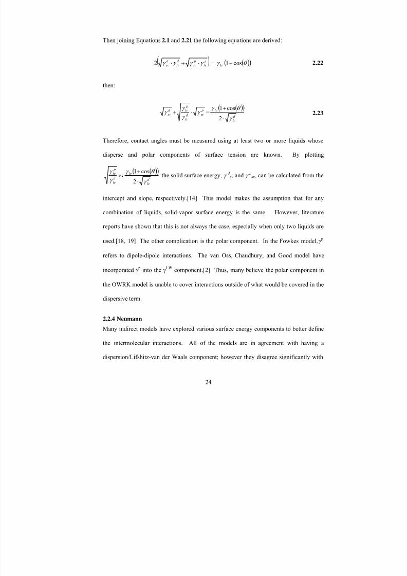
energy is the slope determined by plotting RT ln V N against ( ) 2/1 D
L
a γ ⋅ as shown in Figure
1-1. When a liquid with both polar and dispersive free energy components is used in the
IGC measurements, the vapors will interact differently and points will lie above the
alkane line. The magnitude of this difference is equal to the specific component of the
surface energy ( )SP
AGΔ of the powder material in the column. The electron donor (K D)
and electron acceptor (K A) properties of the materials can then be related to specific
surface energy by:
* AN K DN K G D A
SP
A ⋅+⋅=Δ 1.3
where DN and AN describes the electron donor or base and electron acceptor or acid
properties of the liquids, respectively. Using several probes with dispersion and polar
properties to measure ( )SP
AGΔ , and plotting DN/AN*
against*
/ AN GSP
AΔ , the values of K A
and K D can be calculated for the material of interest. [3, 5]
IGC has been used to evaluate the surface energy differences of different batches of
excipients, crystalline polymorphs, and amorphous material. IGC is an effective method
for investigating the surface energy of powder samples, but IGC is thought to
preferentially probe only the highest energy sites. Also, with polar probes, the
reproducibility of the measurements is questionable because retention times are
inconsistent between sample runs.[4] The biggest reason IGC was not a focus for this
work is because of the inability to measure the surface energy on individual crystalline

7/27/2019 Atomic Force Microscopy Method Development for Surface Energy Analysis
http://slidepdf.com/reader/full/atomic-force-microscopy-method-development-for-surface-energy-analysis 27/365
5
faces. In order to understand the contribution of surface energy during crystallization,
another method will have to be used.

7/27/2019 Atomic Force Microscopy Method Development for Surface Energy Analysis
http://slidepdf.com/reader/full/atomic-force-microscopy-method-development-for-surface-energy-analysis 28/365
6
Figure 1-1: Schematic diagram showing how to determine the dispersion surface energyand the specific surface energy component.
a (γLD)1/2
R T
l n V N −ΔGA
SP

7/27/2019 Atomic Force Microscopy Method Development for Surface Energy Analysis
http://slidepdf.com/reader/full/atomic-force-microscopy-method-development-for-surface-energy-analysis 29/365
7
The most common method for measuring contact angles is by sessile drop. A small drop
of liquid is placed on the surface of a solid from a syringe and recorded with a video
based goniometer. The static contact angle can be measured directly by measuring the
angle between the tangent to the drop surface at the point of contact with the solid and the
horizontal solid surface, Figure 2-1. The advancing and receding angles can be
determined by repeatedly adding or removing the liquid to the forming drop. The process
is recorded and the angles are analyzed by software that is integrated with the contact
angle system. Once the angles are measured, several indirect models have been used to
calculate the surface energy. Most of these models split the total surface energy intodispersion and polar (or acid-base) components, similar to the IGC model. These models
are discussed extensively in Chapter 2.
The contact angle method has been used on powders compressed into tablet compacts
and single crystalline faces. The experimental challenges for contact angle measurements
will be discussed in detail in Chapter 2. The main limitations of this method are, one, the
sessile drop is complicated by the stress at the edge of the contact circle causing
additional surface changes[5, 6], which, in turn, affects the surface energy. Second, the
sessile drop method may not be sensitive enough to detect the change in surface energy
due to the subtle structure change, and large single crystals are needed in order to
measure the contact angle on particular faces.[7, 8]
The major problem with IGC is the instrument’s inability to distinguish the surface
energy of each crystalline face. Sessile drop can measure surface energy on each face,
but the limitations listed above drove the need for development of other methods that can
provide comprehensive surface energy information.

7/27/2019 Atomic Force Microscopy Method Development for Surface Energy Analysis
http://slidepdf.com/reader/full/atomic-force-microscopy-method-development-for-surface-energy-analysis 30/365
8
Atomic force microscopy is a scanning probe measurement based upon the variable
displacement of a cantilever tip as it scans across the topography of a solid surface. The
forces between the solid surface and the tip result in a deformation of the cantilever,
measurable by a spatially resolved photodetector. The instrument is typically operated in
either contact mode, where the cantilever tip is dragged across the surface or in tapping
mode, where the tip is oscillated at a known frequency. However, contact mode is the
only mode that a positive deflection can be measured and adhesion can be studied. The
measured AFM forces are then converted into work of adhesion using either the Johnson-
Kendall-Roberts (JKR) or Deryaguin-Muller-Toporov (DMT) contact mechanics models.The work of adhesion (W) is then defined by surface energy (SE). Thus, the
mathematical sequence for determining surface energy with the AFM is
SE W F →→
The contact mechanics models and surface energy models are discussed in Chapter 4, and
Chapter 3 provides a review of the AFM and the methodology used to measure forces.
The AFM was an attractive tool to use for investigating surface energy because of its
ability to resolve interactions sub-angstrom, on the molecular level, and because of the
various disadvantages of using contact angle and IGC. IGC cannot evaluate single
crystalline faces and the AFM can evaluate a range of materials because of the nanometer
sized tips. While the contact angle can evaluate various surfaces, it is a macroscopic
method, averaging over surface features that can be different within a specific area. For a
surface which is not ideal and inert, it may be difficult to obtain a meaningful surface
energy based on contact angle measurement. For these reasons the following objectives
were investigated to evaluate the capabilities of the AFM.

7/27/2019 Atomic Force Microscopy Method Development for Surface Energy Analysis
http://slidepdf.com/reader/full/atomic-force-microscopy-method-development-for-surface-energy-analysis 31/365
9
1.4 Objectives
1.4.1 Specific Aim 1
The first purpose of this research was to develop the AFM as an analytical method and
determine its viability as a potential technique for measuring surface energies of various
crystal systems. Linearly, this goal was subdivided into five specific tasks: 1) determine
the surface energy of inert materials using a contact angle method and demonstrate its
limitations for determining solid-liquid surface energies, 2) evaluate tip properties of an
AFM probe to calculate forces and evaluate tip sharpness, 3) establish repeatability and a
model for statistical analysis, 4) assess adhesion mechanics models and develop surface
energy models for the AFM, and 5) compare the AFM calculations to contact angle
results. More concisely, these subdivisions were organized to develop and utilize a
reference method for comparison (contact angle), to understand the hardware and
physical considerations of the new method (AFM), to understand and select the most
appropriate scientifically rigorous mathematical and theoretical models for the new
method, and to compare the reference standard with the incumbent method. Much like
any secondary method of analysis, the AFM required correlation to a primary reference
method to establish its position.
1.4.1.1 Determine the surface energy of reference materials using a contact angle
method and demonstrate the limitations for determining solid-liquid surface
energies.
To address specific aim 1, contact angle was used to determine the surface energy of
reference materials, and thereby, its limitations were evaluated for measuring solid-liquid

7/27/2019 Atomic Force Microscopy Method Development for Surface Energy Analysis
http://slidepdf.com/reader/full/atomic-force-microscopy-method-development-for-surface-energy-analysis 32/365
10
surface energies. Graphite and mica were selected as the reference-surface test systems,
and the sessile drop method was used to measure static, advancing, and receding contact
angles. Water, ethylene glycol, formamide, and diiodomethane were selected as the
liquids to measure wettability and spreadability on the graphite and mica surfaces. These
liquids were chosen to investigate how relative degrees of polarity (water > formamide >
ethylene glycol > diiodomethane) affected their respective contact angles. Typical
indirect models were used to determine the solid-vapor surface energy of the two surfaces
and then the solid-liquid surface energies were calculated from Young’s equation.
1.4.1.2 Evaluate tip properties of an AFM probe to calculate forces and evaluate tip
sharpness.
To calculate the force of adhesion with an AFM measurement, the spring constant of the
cantilever needed to be determined. One destructive method and one nondestructive
method were tested, each of which will be described in detail in subsequent chapters. Tip
radii were measured with SEM images from five probes and averaged. Then a novel
nondestructive method was used relying on tip reconstruction by scanning a rough image
and evaluating this image with calculations in SPIP software. Tip radii are continually
evaluated with this technique to determine when the tip becomes blunt and unusable.
1.4.1.3 Establish reproducibility among AFM measurements and develop a
statistical model for error analysis.
Parameters were tested to increase repeatability of the force measurements at different
locations on a discrete sample and with the same tip. The parameters tested included
scan size, scan rate, forces applied, and contact area. Once the forces were measured, a

7/27/2019 Atomic Force Microscopy Method Development for Surface Energy Analysis
http://slidepdf.com/reader/full/atomic-force-microscopy-method-development-for-surface-energy-analysis 33/365
11
repeated measure mixed model statistical analysis was performed to summarize the AFM
data. 1.4.1.4 Assess adhesion mechanics models and develop surface energy models for the
AFM.
First, the three adhesion mechanics models that have been developed were evaluated.
These models are reviewed in Chapter 4 lending to an understanding of the most
applicable model for samples in this study and determining applicability in future studies.
Next, four surface energy models were developed. Since there is currently no method to
directly measure surface energy, the advantages, assumptions, and limitations are
presented.
1.4.1.5 Compare AFM calculations to contact angle results
All forces were measured using the same liquids from contact angle measurements.
Environmental conditions were controlled to increase repeatability, including ambient,
zero percent relative humidity achieved by purging the chamber with nitrogen gas, dried
hygroscopic solvents (ethylene glycol and formamide), and controlled hydration of
solvents. The repeated measures mixed model statistical analysis was used to identify
any difference in the measurements and what the possible sources of deviation are.
1.4.2 Specific Aim 2
The second purpose of this research was to apply the methodology and mathematical
models developed on references surfaces, such as mica or graphite, to organic crystalline
surfaces.

7/27/2019 Atomic Force Microscopy Method Development for Surface Energy Analysis
http://slidepdf.com/reader/full/atomic-force-microscopy-method-development-for-surface-energy-analysis 34/365
12
1.4.2.1 Determine the surface energy of aspirin using the contact angle method.
Sessile drop was used to measure the contact angles on the two major faces of aspirin.
Three liquids with different properties were used to explore wettability. The same
indirect models were used to determine the solid-vapor surface energy of the two surfaces
and then the solid-liquid surface energies were calculated from Young’s equation.
1.4.2.2 Use the methods developed on inert surfaces with the AFM and apply them
to the crystalline measurements.
Forces were measured in only controlled relative humidity to determine solid-vapor
surface energy because solvent trapped in the crystals and water vapor that can adsorbed
on the surface in ambient conditions prevented engagement of the microscope. Forces
were pure aqueous solution, but dissolution on the surface of the crystalline was too rapid
because of solubility. Hence, the forces were measured in varying solute concentrations
on the major faces of aspirin until saturation was reached. Stability and repeatability in
measurements were observed at saturation and above.
The goal in the following chapters is to present the theory and methods of contact angle
and AFM. In these chapters, the results from each specific aim will be presented and
discussed.
Copyright © Clare Aubrey Medendorp 2011

7/27/2019 Atomic Force Microscopy Method Development for Surface Energy Analysis
http://slidepdf.com/reader/full/atomic-force-microscopy-method-development-for-surface-energy-analysis 35/365
13
Chapter 2 – Contact Angle
In this chapter, the definition of contact angle and a literature review on the evaluation of
indirect models developed to calculate surface energy is presented. Then, the sessile drop
method is used to determine the contact angles of two reference samples, mica and
graphite, so that the solid-vapor and solid-liquid surface energy of these samples can be
calculated. The final sections of this chapter present the contact angle measurements on
mica and graphite, the surface energy results determined from the indirect models, and
the drawbacks of using the contact angle method.
2.1 Contact Angle and Young’s Equation
Contact angle is defined as the angle, θ, formed between the liquid-vapor, solid-vapor,
and liquid-solid interfaces at a three phase contact line (Figure 2-1). In principle, on a
smooth, homogeneous, rigid, isotropic solid surface, the equilibrium contact angle of a
pure liquid is a unique quantity[9], and Young’s equation is obeyed and can be defined
by:
)cos(θ γ γ γ lvslsv += 2.1
where γsv is the solid-vapor interfacial free energy, γsl is the solid-liquid interfacial free
energy, and γlv is the liquid-vapor interfacial tension (for liquids, often called surface
tension).

7/27/2019 Atomic Force Microscopy Method Development for Surface Energy Analysis
http://slidepdf.com/reader/full/atomic-force-microscopy-method-development-for-surface-energy-analysis 36/365
14
Figure 2-1: Sessile drop of a liquid on a solid demonstrating the three-phase boundary.
Solid
Vapor γsvsl
γlv
θ
Solid
Vapor γsvsl
γlv
θ
7/27/2019 Atomic Force Microscopy Method Development for Surface Energy Analysis
http://slidepdf.com/reader/full/atomic-force-microscopy-method-development-for-surface-energy-analysis 37/365
15
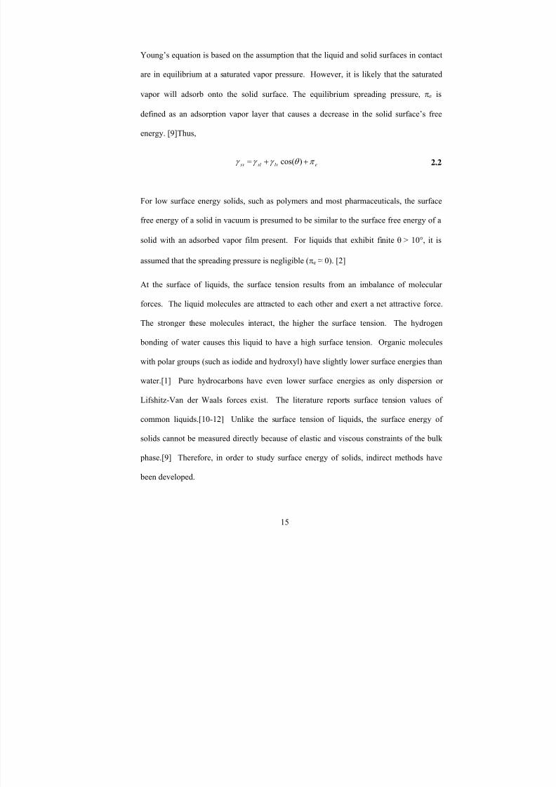
Young’s equation is based on the assumption that the liquid and solid surfaces in contact
are in equilibrium at a saturated vapor pressure. However, it is likely that the saturated
vapor will adsorb onto the solid surface. The equilibrium spreading pressure, πe is
defined as an adsorption vapor layer that causes a decrease in the solid surface’s free
energy. [9]Thus,
elvslsv π θ γ γ γ ++= )cos( 2.2
For low surface energy solids, such as polymers and most pharmaceuticals, the surface
free energy of a solid in vacuum is presumed to be similar to the surface free energy of a
solid with an adsorbed vapor film present. For liquids that exhibit finite θ > 10°, it is
assumed that the spreading pressure is negligible (πe ≈ 0). [2]
At the surface of liquids, the surface tension results from an imbalance of molecular
forces. The liquid molecules are attracted to each other and exert a net attractive force.
The stronger these molecules interact, the higher the surface tension. The hydrogen
bonding of water causes this liquid to have a high surface tension. Organic molecules
with polar groups (such as iodide and hydroxyl) have slightly lower surface energies than
water.[1] Pure hydrocarbons have even lower surface energies as only dispersion or
Lifshitz-Van der Waals forces exist. The literature reports surface tension values of
common liquids.[10-12] Unlike the surface tension of liquids, the surface energy of
solids cannot be measured directly because of elastic and viscous constraints of the bulk
phase.[9] Therefore, in order to study surface energy of solids, indirect methods have
been developed.
7/27/2019 Atomic Force Microscopy Method Development for Surface Energy Analysis
http://slidepdf.com/reader/full/atomic-force-microscopy-method-development-for-surface-energy-analysis 38/365
16
2.2 Review of the Geometric Mean and Indirect Models
In the past 40 years, a series of semi-empirical analytical models have been developed to
relate contact angle data to solid surface free energy. Surface energy component
approaches, such as Fowkes[13], Owens-Wendt-Rabel-Kaelble[14], Chen-Chang[15],
and van Oss et al[16] have been used to evaluate the surface free energy components of
many solid materials. All of the models are based on the assumption that the surface free
energy of a solid and/or a liquid consists of independent or partially independent
components. These independent components represent different types of intermolecular
interactions. In this review, the most common indirect models will be discussed and
evaluated.
Before the indirect models could be formulated, it was recognized that one of the
unknowns in Young’s equation needed to be eliminated. This was possible through the
use of the geometric mean combining rule.[2, 9] It was hypothesized that the free energy
of adhesion is equal to the geometric mean of the free energies of cohesion of the
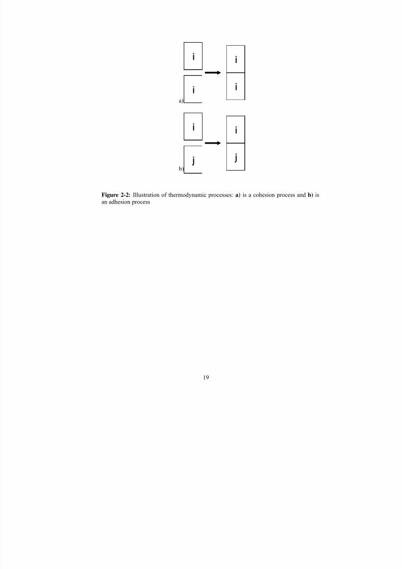
individual components. The free energy of cohesion, ΔGc, is the change of the reversible
process of bringing two identical bodies, Figure 2-2a, together so that:
γ 2−=−=Δ ccW G 2.3
However, when two dissimilar bodies, Figure 2-2b, are brought together reversibly, the
free energy change of adhesion, ΔGa12 , is:
21121212 γ γ γ −−=−=Δ aaW G 2.4
7/27/2019 Atomic Force Microscopy Method Development for Surface Energy Analysis
http://slidepdf.com/reader/full/atomic-force-microscopy-method-development-for-surface-energy-analysis 39/365
17
where, phases 1 and 2 represent the separate phases, and 12 represents the interface
between phase 1 and phase 2.
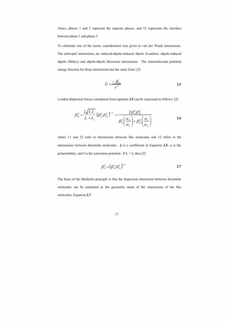
To eliminate one of the terms, consideration was given to van der Waals interactions.
The principal interactions are induced-dipole-induced dipole (London), dipole-induced
dipole (Debye) and dipole-dipole (Keesom) interactions. The intermolecular potential
energy function for these interactions has the same form: [2]
6
12
r
U β −
= 2.5
London dispersion forces considered from equation 2.5 can be expressed as follows: [2]
( )
⎟⎟ ⎠
⎞⎜⎜⎝
⎛ +⎟⎟
⎠
⎞⎜⎜⎝
⎛ =
+=
2
122
1
211
22112/1
2211
21
2112
22
α
α β
α
α β
β β β β β
d d
d d
d d d
I I
I I
2.6
where 11 and 22 refer to interactions between like molecules and 12 refers to the
interactions between dissimilar molecules. β is a coefficient in Equation 2.5, α is the
polarizability, and I is the ionization potential. If I1 ≈ I2 then [2]
( ) 2/1
221112d d d β β β = 2.7
The basis of the Berthelot principle is that the dispersion interaction between dissimilar
molecules can be estimated as the geometric mean of the interactions of the like
molecules, Equation 2.7.

7/27/2019 Atomic Force Microscopy Method Development for Surface Energy Analysis
http://slidepdf.com/reader/full/atomic-force-microscopy-method-development-for-surface-energy-analysis 40/365
18
Thus, binary interactions for van der Waals components can be determined from the pure
components by:
( ) ( )2/1
2211
2/1
221112 2 d d d d d GGG γ γ ΔΔ−=ΔΔ=Δ 2.8
The combining rule makes it possible to predict properties of the 12 interface from the
separate properties of phase 1 and 2 phases. With this assumption it is possible to
eliminate γ12 from Young’s equation and develop indirect models.[1, 2, 9, 17]
7/27/2019 Atomic Force Microscopy Method Development for Surface Energy Analysis
http://slidepdf.com/reader/full/atomic-force-microscopy-method-development-for-surface-energy-analysis 41/365
19
Figure 2-2: Illustration of thermodynamic processes: a) is a cohesion process and b) isan adhesion process
i
i
i
i
i
i
i
i
i
j
i
j
i
j
i
j
a)
b)

7/27/2019 Atomic Force Microscopy Method Development for Surface Energy Analysis
http://slidepdf.com/reader/full/atomic-force-microscopy-method-development-for-surface-energy-analysis 42/365
20
2.2.1 Fowkes
Initially, Fowkes proposed that a solid’s surface free energy, γs, could be considered to be
the sum of a dispersive, (London, γd), an apolar, (Keesom, γ p), an induction, (Debye, γind),
and a hydrogen bonding (γh) component such that:[9]
hind pd γ γ γ γ γ +++= 2.9
However, Fowkes finally settled on two dominant terms:
ABd γ γ γ += 2.10
where d is the dispersive and AB is the acid-base component. In Fowkes equation, the
acid-base component is comprised of the polar, induction, and hydrogen bonding
interactions.[2] Fowkes reason for the integration was supported by proving that the
contributions of dipole-dipole attraction (γ p) and dipole-induced dipole attraction (γind)
were significantly smaller than the dispersive surface energy component (γd).[2, 9]
2.2.2 Van Oss, Chaudhury, Good
Van Oss, Chaudhury, and Good explored Fowkes’ model in more detail, and after
evaluating Lifshitz calculations and theory, arrived at a different conclusion. Their
investigation showed it is not possible to separate out a γ p or γind term. The only
measurable interaction is the Lifshitz-van der Waals, γLW, which includes all
electromagnetic interactions together, γd, γ p, and γind. Therefore the model equation
becomes:[2, 9]

7/27/2019 Atomic Force Microscopy Method Development for Surface Energy Analysis
http://slidepdf.com/reader/full/atomic-force-microscopy-method-development-for-surface-energy-analysis 43/365
21
AB LW γ γ γ += 2.11
Using the geometric mean and parameters from Young’s equation, the components in
Equation 2.11 can be broken down further to evaluate the interaction between dissimilar
bodies:
LW
lv
LW
sv
LW
lv
LW
sv
LW W W W sl
γ γ 2== ,
+−−++−−+ +=+= lvsvlvsvlvsvlvsv
AB W W W W W sl
γ γ γ γ 22
2.12
In the development of the acid-base term it was recognized that a molecule can be
bipolar, containing both a Lewis acid, γ+, and a Lewis base, γ-, as with water. If either the
acidic or basic property is negligible, then the substance is termed monopolar.[2] When
the substance does not exhibit either acidic or basic properties, it is considered apolar.
Hydrogen bonding is another example of a Lewis acid and Lewis base interaction.[9]
Therefore, this model provides more insight as to whether a substance can accept or
donate electrons.
To determine γsv, Equations 2.12 are combined to produce:
+−−+ −−−+= lvsvlvsv
LW
lv
LW
svlvsvsl γ γ γ γ γ γ γ γ γ 222 2.13
Then, combining Equations 2.1 and 2.13 the following equations are derived:
( )( )θ γ γ γ γ γ γ γ cos1222 +=++ +−−+lvlvsvlvsv
LW
lv
LW
sv 2.14

7/27/2019 Atomic Force Microscopy Method Development for Surface Energy Analysis
http://slidepdf.com/reader/full/atomic-force-microscopy-method-development-for-surface-energy-analysis 44/365
22
In order to use the van Oss et. al. model, at least three liquids must be used to measure
contact angles. First an apolar liquid is chosen and Equation 2.14 is reduced to: [2, 9, 12,
16]
( )( )θ γ γ γ cos12 += lv
LW
lv
LW
sv 2.15
The Lifshitz-van der Waals component can be calculated from a single contact angle
measurement. Once the LW
svγ is known, the acid-base components can be calculated
using the data from the other two liquids and Good’s equations (a determinant
method).[2, 9, 12, 16]
DE CF
AE BC s −
−=−γ ,
DE CF
BD AF s −
−=+γ
( ) LW LW
s A 22 2)cos(1 γ γ θ γ −+=
( )
LW LW
s B 33 2)cos(1 γ γ θ γ −+=
−= 22 γ C , += 22 γ D
−= 32 γ E , += 32 γ F
2.16
Negative and small values of +sγ occur often. The small values usually can be taken as
zero, but a definitive method for handling negative numbers has not yet been proposed.[2,
9] It is possible that the phenomenon is real and thus the equation to determine the acid
base component is written:
7/27/2019 Atomic Force Microscopy Method Development for Surface Energy Analysis
http://slidepdf.com/reader/full/atomic-force-microscopy-method-development-for-surface-energy-analysis 45/365
23
−+= ss
AB
s γ γ γ 2 2.17
One criticism made of this model is the numerical designation made for water,
2mJ/m5.25== −+ γ γ . Most researchers also agree that when using this model, the
calculated values of surface free energy components depend upon the choice of
liquids.[2] There is less dependence when more liquids are used for the calculation.
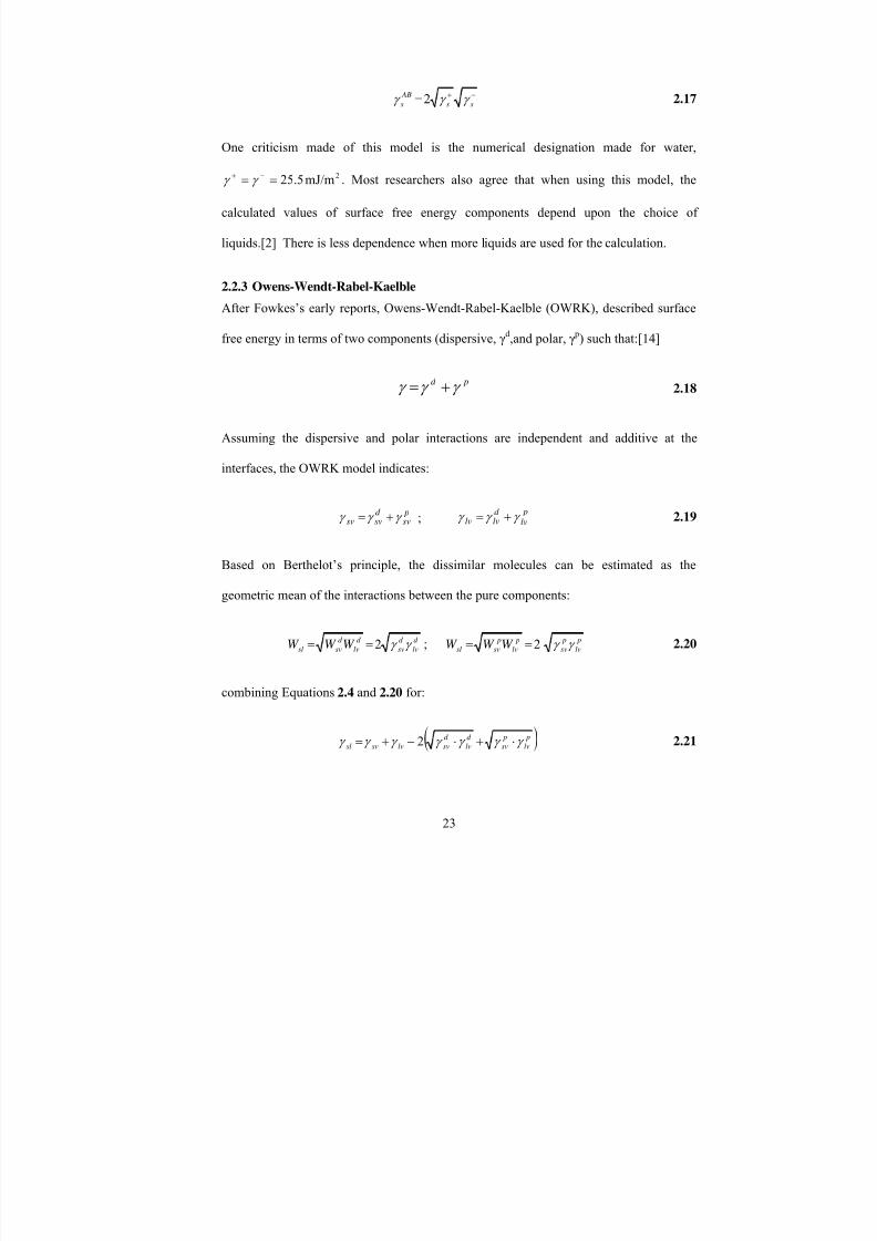
2.2.3 Owens-Wendt-Rabel-Kaelble
After Fowkes’s early reports, Owens-Wendt-Rabel-Kaelble (OWRK), described surface
free energy in terms of two components (dispersive, γd,and polar, γ p) such that:[14]
pd γ γ γ += 2.18
Assuming the dispersive and polar interactions are independent and additive at the
interfaces, the OWRK model indicates:
psv
d svsv γ γ γ += ;
p
lvd lvlv γ γ γ += 2.19
Based on Berthelot’s principle, the dissimilar molecules can be estimated as the
geometric mean of the interactions between the pure components:
d
lv
d
sv
d
lv
d
svsl W W W γ γ 2== ; p
lv
p
sv
p
lv
p
svsl W W W γ γ 2== 2.20
combining Equations 2.4 and 2.20 for:
( ) p
lv
p
sv
d
lv
d
svlvsvsl γ γ γ γ γ γ γ ⋅+⋅−+= 2 2.21
7/27/2019 Atomic Force Microscopy Method Development for Surface Energy Analysis
http://slidepdf.com/reader/full/atomic-force-microscopy-method-development-for-surface-energy-analysis 46/365
24
Then joining Equations 2.1 and 2.21 the following equations are derived:
( )( )θ γ γ γ γ γ cos12 +=⋅+⋅ lv
p
lv
p
sv
d
lv
d
sv 2.22
then:
( )( )d
lv
lv p
svd
lv
p
lvd
sv
γ
θ γ γ
γ
γ γ
⋅
+=⋅+
2
cos1 2.23
Therefore, contact angles must be measured using at least two or more liquids whose
disperse and polar components of surface tension are known. By plotting
( )( )d
lv
lv
d
lv
p
lv vsγ
θ γ
γ
γ
⋅
+
2
cos1. the solid surface energy, γ d
sv and γ psv, can be calculated from the
intercept and slope, respectively.[14] This model makes the assumption that for any
combination of liquids, solid-vapor surface energy is the same. However, literature
reports have shown that this is not always the case, especially when only two liquids are
used.[18, 19] The other complication is the polar component. In the Fowkes model, γ p
refers to dipole-dipole interactions. The van Oss, Chaudhury, and Good model have
incorporated γ p into the γLW component.[2] Thus, many believe the polar component in
the OWRK model is unable to cover interactions outside of what would be covered in the
dispersive term.
2.2.4 Neumann
Many indirect models have explored various surface energy components to better define
the intermolecular interactions. All of the models are in agreement with having a
dispersion/Lifshitz-van der Waals component; however they disagree significantly with
7/27/2019 Atomic Force Microscopy Method Development for Surface Energy Analysis
http://slidepdf.com/reader/full/atomic-force-microscopy-method-development-for-surface-energy-analysis 47/365
25
the definition of the second component. Neumann et al. tried to improve this problem
using the equation of state and not separate interactions.
The equation of state is simply:
( )lvsvsl f γ γ γ ,= 2.24
Since both γsv and γsl in Young’s equations are parameters to be determined, an additional
equation providing a relation among the surface tensions was required. The approach
taken by Neumann and his coworkers does not consider the molecular origins of surface
energy like previous models. The method developed is an extension and modification of
the Berthelot Rule, (Equation 2.8): [19, 20]
2)(2 svlveW lvsvγ γ β
γ γ −−= 2.25
where β is an unknown constant added as part of the modification and now is an
empirical constant that has been determined to be 1.247 x 10⁻⁴
m4
mJ-2
. The modification
was made because the geometric mean overestimates the strength of the unlike-pair
interactions. Thus, a modification factor is added to decrease the function of the
difference (γlv – γsv) and is equal to unity when the difference is zero.
Then substituting Equation 2.25 into Equation 2.4 gives:
2)( svlvelvsvlvsvslγ γ β
γ γ γ γ γ −−−+= 2.26
Combining Equation 2.26 with Young’s equation (Equation 2.1) and simplifying yields:

7/27/2019 Atomic Force Microscopy Method Development for Surface Energy Analysis
http://slidepdf.com/reader/full/atomic-force-microscopy-method-development-for-surface-energy-analysis 48/365
26
2)(21)cos( svlvelv
sv γ γ β
γ
γ θ
−−+−= 2.27
In Equation 2.27, β and γsv are the unknowns and can be determined by finding the best
fit from the measured data using nonlinear least-squares analysis. When simplified
equation 2.27 becomes:
( )2ln2
1
2
1)cos(ln svlvsvlv γ γ β γ
θ γ −−=⎥
⎦
⎤⎢⎣
⎡⎟ ⎠
⎞⎜⎝
⎛ + 2.28
where:
⎥⎦
⎤⎢⎣
⎡⎟ ⎠
⎞⎜⎝
⎛ +=
2
1)cos(ln
θ γ lvY ; lv X γ = 2.29
This model assumes that for a group of liquids γsv will be constant. This model is based
on molecular interactions of like pairs and specifically long range dispersion forces. The
dispersion energy coefficient for two dissimilar molecules can be expressed in terms of
the similar molecules, which is the basis for the geometric mean. The main criticism of
this model is the contrast with the statistical thermodynamic approach used by Fowkes,
OWRK, and van Oss, Chaudhury, and Good. Since this model does not consider the
molecular origins of surface tension, no statistical mechanical insight is gained.[2]
2.2.5 Model Summary
In summary, several indirect models have been developed and can be used to determine
solid vapor surface energy. Once γsv
is determined from an indirect model, its value
along with the contact angle determined from various liquids can be substituted back into
7/27/2019 Atomic Force Microscopy Method Development for Surface Energy Analysis
http://slidepdf.com/reader/full/atomic-force-microscopy-method-development-for-surface-energy-analysis 49/365
27
Young’s Equation to calculate γsl. So far there is no unified agreement on one universal
indirect model. There are two unknowns in Young’s equation and the use of the
geometric mean helps eliminate one unknown. The geometric mean overestimates
surface energy; therefore modifications have been made and surface energy components
have been evaluated. Neumann found an empirical modification to correct for the
overestimation. This has been an approach mainly used when mixing liquids. [21]Van
Oss et al. and OWRK evaluated the total surface energy based on components. The total
surface energy was defined by dispersive/van der Waals and polar/AB. To evaluate the
binary interactions of each component, the geometric mean was used. The geometric
mean was developed for van der Waals interactions and not the polar/AB interactions. In
order to use the geometric mean with the polar and AB components, the assumption
made is that the pure components’ differences in electronic properties and molecular size
are small. [21] Fowkes found that the geometric mean may not satisfactorily describe
polar liquid/solid interactions and noted that a direct proportionality between γsl p and γl
p
maybe more accurate. However, until it is possible to directly measure surface energy,
indirect models will have to be used. Hence, consideration should be given to the
assumptions each model makes before applying that model to a particular surface of
interest. In this chapter, the OWRK, van Oss-Chadhury-Good, and Neumann indirect
models will be applied to contact angle data collected on mica and graphite to evaluate
similarities and discrepancies between the models.
2.3 Experimental Challenges of Contact Angles Measurements
When using sessile drop and other methods to measure contact angles, there are various
challenges that must not be ignored. The factors that can effect the contact angle

7/27/2019 Atomic Force Microscopy Method Development for Surface Energy Analysis
http://slidepdf.com/reader/full/atomic-force-microscopy-method-development-for-surface-energy-analysis 50/365
28
measurements are surface heterogeneity and roughness, solvent purity, temperature, and
surface stability. This section reviews some limitations experienced with contact angle
measurements.
2.3.1 Contact Angle Hysteresis
In section 2.1, the assumption was made that Young’s equation holds and an equilibrium
angle can be measured if the solid surface is smooth, homogeneous, rigid, and isotropic.
However, this is not frequently seen. Typically there is appreciable hysteresis observed.
Hysteresis is defined as the difference between the advancing angle, θa, and the receding
angle, θr
r a H θ θ −= 2.30
Hysteresis of one or two degrees has been regarded as negligible and within the
uncertainty of the experimental measurement. However a hysteresis of 10º or larger has
been observed in some cases that cannot be attributed to the measurement.[9] The
theoretical basis for hysteresis is the failure of the system to meet the conditions of
ideality. Examples of non-ideality are roughness and heterogeneity. When hysteresis
occurs, the advancing contact angle is used to determine the surface energy.[9] Good
stated that when an equilibrium angle is observed on a homogeneous, flat surface with
lower free energy components, the maximum contact angle value is taken, which is the
advancing contact angle.[9, 17] For example, on a patchy (heterogeneous) surface whose
areas have different surface energies, and the advancing angle is greater than the receding
angle, which is most commonly observed, the equilibrium angle will be the advancing

7/27/2019 Atomic Force Microscopy Method Development for Surface Energy Analysis
http://slidepdf.com/reader/full/atomic-force-microscopy-method-development-for-surface-energy-analysis 51/365
29
angle. When there are smaller surface energy components on the surface, the liquid's
cohesive forces cannot be overcome. Through this phenomenon, a larger contact angle is
observed. The large contact is the advancing angle. The receding angle is observed as
the liquid is retracted from the surface. The contact angle software allows control over
the amount of liquid and the rates of application onto a surface and retraction from the
surface. The entire experiment is recorded with a video based goniometer and the contact
angle software analyzes the angles. The advancing angle is observed when the liquid
stops spreading and the receding angle is measured as the liquid is retracted.
2.3.2 Contact angle measurements with hygroscopic solvents and additive solutions
The uptake of moisture in the liquid can affect the interaction the hygroscopic liquid has
with the surface which therefore, influences the resultant contact angle. In Section 2.5.3,
the presence of water will be evaluated with two hygroscopic solvents, ethylene glycol
and formamide.
With contact angle measurements, studies have shown that only the use of pure solvents
will provide unambiguous results. In the literature, surface tensions are available for only
pure solvents. While the additions of additives or surfactants can affect the surface
tension of a liquid, it is thought that the adsorption is not equally distributed across the
three interfaces when the solution is dropped on a surface.[17, 22] Studies done in the
Zografi lab illustrated the nonequivalent adsorption in two ways: [22]
1. The liquid-vapor surface energy (γlv), also known as the surface tension of a liquid, is
different for a pure liquid and that same liquid with an additive or surfactant, and

7/27/2019 Atomic Force Microscopy Method Development for Surface Energy Analysis
http://slidepdf.com/reader/full/atomic-force-microscopy-method-development-for-surface-energy-analysis 52/365
30
2. The liquid-vapor surface energy (γlv) is not different for a pure liquid and that same
liquid with an additive or surfactant.
For the first case, if the surface tension of a liquid is different between a pure solvent and
a solution, but the surfactant or additive in the solution does not wet or adsorb well at the
solid-liquid surface, there won't be a change in γsl, as compared to the γsl measured by the
pure solvent. This could mean that the particular additive or surfactant used has little
interaction with the surface or is a poorer wetting agent. However, when other pure
liquids with distinctive γlv are used, a difference is observed in the contact angles. Thus
the solid-liquid interaction results in different γsl. It is difficult to say that no change in γsl
is just because of poor wetting. It could also mean that the additive is not dispersed
homogeneously across the three interfaces.
For the second case, the surface tension of the solution is the same as the pure liquid, but
there is a change in the solid-liquid surface energy from an increase or decrease in the
contact angle. In this instance, it is unclear if the adsorption of the surfactant or additive
is affected by a strong interaction with the surface or a lack of interaction at the liquid-
vapor interface.
All of these results show that the relative adsorption of an additive or surfactant to the
liquid-vapor interface and the solid-liquid interfaces is critical to understanding the
wetting characteristics. Therefore, the study of contact angles will not yield how
additives can affect crystal growth.
7/27/2019 Atomic Force Microscopy Method Development for Surface Energy Analysis
http://slidepdf.com/reader/full/atomic-force-microscopy-method-development-for-surface-energy-analysis 53/365
31
2.3.3 Temperature effect on contact angle measurements
Studies have been conducted to evaluate how temperature affects surface tension of
liquid and surface energy of solids. For solvents, as temperature increases, the surface
tension of the liquid decreases.[1] Intuitively, if there is an increase in thermal motion of
molecules, there would be a decrease in the surface tension. Since indirect surface
energy models evaluate various surface energy components, the solvent’s surface tension
terms have to be reevaluated at varying temperatures. However, for solids, the
temperature effect has been more difficult to study with the indirect models. The
dispersive forces, which exist in all types of matter, depend on electrical properties of the
elements involved and the distance between them, and therefore, are independent of
temperature.[23] Thus, it was established that only the polar term (which was indicated
in this study to include all non-dispersive forces, such as Lewis acid-base interactions)
decreases with an increase in temperature.[23] Therefore, the polar/AB surface tension
terms at certain temperatures must be found in the literature or measured if temperatures
deviate from reported values. The decrease in solid-vapor surface energy should be less
than what is observed for a liquid because of elastic and viscous restraints of the bulk
phase. McGuire saw an insignificant change in the polar work of adhesion between 30
and 40 degrees centigrade on copper, stainless steel, high density polyethylene, and
polytetrafluoroethylene.[23] Fowkes and Harkin stated that the angles between water and
graphite and water and paraffin increase by 0.06 per degree centigrade with an increase in
temperature. Results from this work will show that 2 to 5 degree contact angle
differences do not significantly change the solid-vapor surface energy. So these studies

7/27/2019 Atomic Force Microscopy Method Development for Surface Energy Analysis
http://slidepdf.com/reader/full/atomic-force-microscopy-method-development-for-surface-energy-analysis 54/365
32
would indicate temperature control in ambient room conditions (15 – 30 ºC) is
unnecessary.[24]
2.3.4 Contact angles on deformable surfaces
Some solids can be described as rigid and insoluble. For these solids, the vertical
component (not shown in Figure 2-1) of surface tension is resisted by elastic distortions
of the solid, which are generally regarded as negligible. However, for solids that cannot
be described in this way, high experimental temperatures or high solubility in a particular
solvent can lead to solution precipitation or some local diffusion. When this happens, a
small ridge can develop at the triple junction (Figure 2-3).[6] When measuring contact
angles, distinction is not made on surfaces containing ridges. If the ridge is present, the
contact angle will be affected, and it is hard to get an accurate surface energy
determination. The possible formation of a ridge can be a big risk when measuring
contact angles with solvents that can dissolve pharmaceutical materials. As a result, this
presents another experimental challenge with contact angle measurements.

7/27/2019 Atomic Force Microscopy Method Development for Surface Energy Analysis
http://slidepdf.com/reader/full/atomic-force-microscopy-method-development-for-surface-energy-analysis 55/365
33
Figure 2-3: Geometry of a liquid drop on a large, isotropic solid depends on the contactline. Initially the solid is rigid (a). Subsequently, a small ridge will form (b) and growthof the perturbation will eventually reach equilibrium (c).[6]

7/27/2019 Atomic Force Microscopy Method Development for Surface Energy Analysis
http://slidepdf.com/reader/full/atomic-force-microscopy-method-development-for-surface-energy-analysis 56/365
34
2.4 Methodology for the Evaluation of Indirect Models on Inert Surfaces
The sessile drop method will be used since it has become the “gold standard” for surface
energy determination, and it is capable of evaluating individual crystalline faces. [7,
25]This section will discuss the methodology used in to measure contact angles.
2.4.1 Inert surfaces
Mica (Ted Pella, Inc., Redding, CA) and highly-oriented pyrolytic graphite (HOPG)
(Digital Instruments, Santa Barbara, CA) were chosen for model validation standards
because the surfaces are free from major defects, relatively smooth, homogeneous, and
inert. Also, the surface properties of these two samples are different so polar and/or
nonpolar interactions can be tested to identify the AFM’s limitation. Studying polar and
nonpolar surfaces is an ongoing challenge with the contact angle method. The different
surface interactions are what triggered the development of several indirect models
mentioned in the previous sections.[9] Before taking a measurement, mica and graphite(HOPG) were cleaved to expose fresh faces and secured on a microscope slide using
adhesive tape.
2.4.2 Contact angle measurements
The contact angles were obtained using a video-based contact angle system (OCA, Future
Digital Scientific Co., Bethpage, NY). First, static contact angles were measured. Drops
(5μL) of water, diiodomethane, and formamide or ethylene glycol were dispensed using a
motor driven syringe. The surface tensions of these liquids are listed in Table 2-1.[2]
The indirect model component values are included in the table. Water contact angles
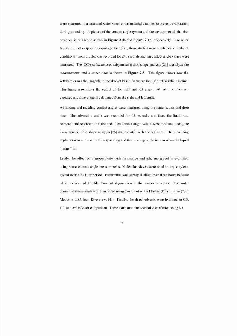
7/27/2019 Atomic Force Microscopy Method Development for Surface Energy Analysis
http://slidepdf.com/reader/full/atomic-force-microscopy-method-development-for-surface-energy-analysis 57/365
35
were measured in a saturated water vapor environmental chamber to prevent evaporation
during spreading. A picture of the contact angle system and the environmental chamber
designed in this lab is shown in Figure 2-4a and Figure 2-4b, respectively. The other
liquids did not evaporate as quickly; therefore, those studies were conducted in ambient
conditions. Each droplet was recorded for 240 seconds and ten contact angle values were
measured. The OCA software uses axisymmetric drop shape analysis [26] to analyze the
measurements and a screen shot is shown in Figure 2-5. This figure shows how the
software draws the tangents to the droplet based on where the user defines the baseline.
This figure also shows the output of the right and left angle. All of these data arecaptured and an average is calculated from the right and left angle.
Advancing and receding contact angles were measured using the same liquids and drop
size. The advancing angle was recorded for 45 seconds, and then, the liquid was
retracted and recorded until the end. Ten contact angle values were measured using the
axisymmetric drop shape analysis [26] incorporated with the software. The advancing
angle is taken at the end of the spreading and the receding angle is seen when the liquid
“jumps” in.
Lastly, the effect of hygroscopicity with formamide and ethylene glycol is evaluated
using static contact angle measurements. Molecular sieves were used to dry ethylene
glycol over a 24 hour period. Formamide was slowly distilled over three hours because
of impurities and the likelihood of degradation in the molecular sieves. The water
content of the solvents was then tested using Coulometric Karl Fisher (KF) titration (737,
Metrohm USA Inc., Riverview, FL). Finally, the dried solvents were hydrated to 0.5,
1.0, and 5% w/w for comparison. These exact amounts were also confirmed using KF.
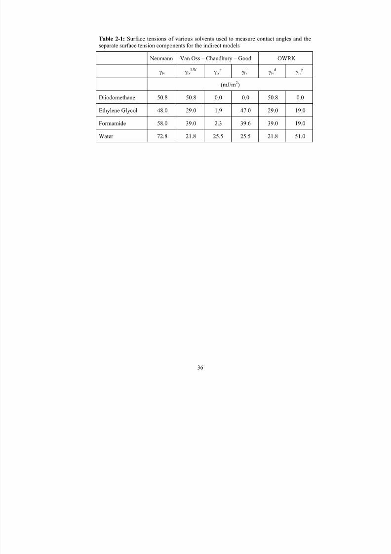
7/27/2019 Atomic Force Microscopy Method Development for Surface Energy Analysis
http://slidepdf.com/reader/full/atomic-force-microscopy-method-development-for-surface-energy-analysis 58/365
36
Table 2-1: Surface tensions of various solvents used to measure contact angles and theseparate surface tension components for the indirect models
Neumann Van Oss – Chaudhury – Good OWRK
γlv γlv
LW
γlv
+
γlv
-
γlv
d
γlv
p
(mJ/m2)
Diiodomethane 50.8 50.8 0.0 0.0 50.8 0.0
Ethylene Glycol 48.0 29.0 1.9 47.0 29.0 19.0
Formamide 58.0 39.0 2.3 39.6 39.0 19.0
Water 72.8 21.8 25.5 25.5 21.8 51.0
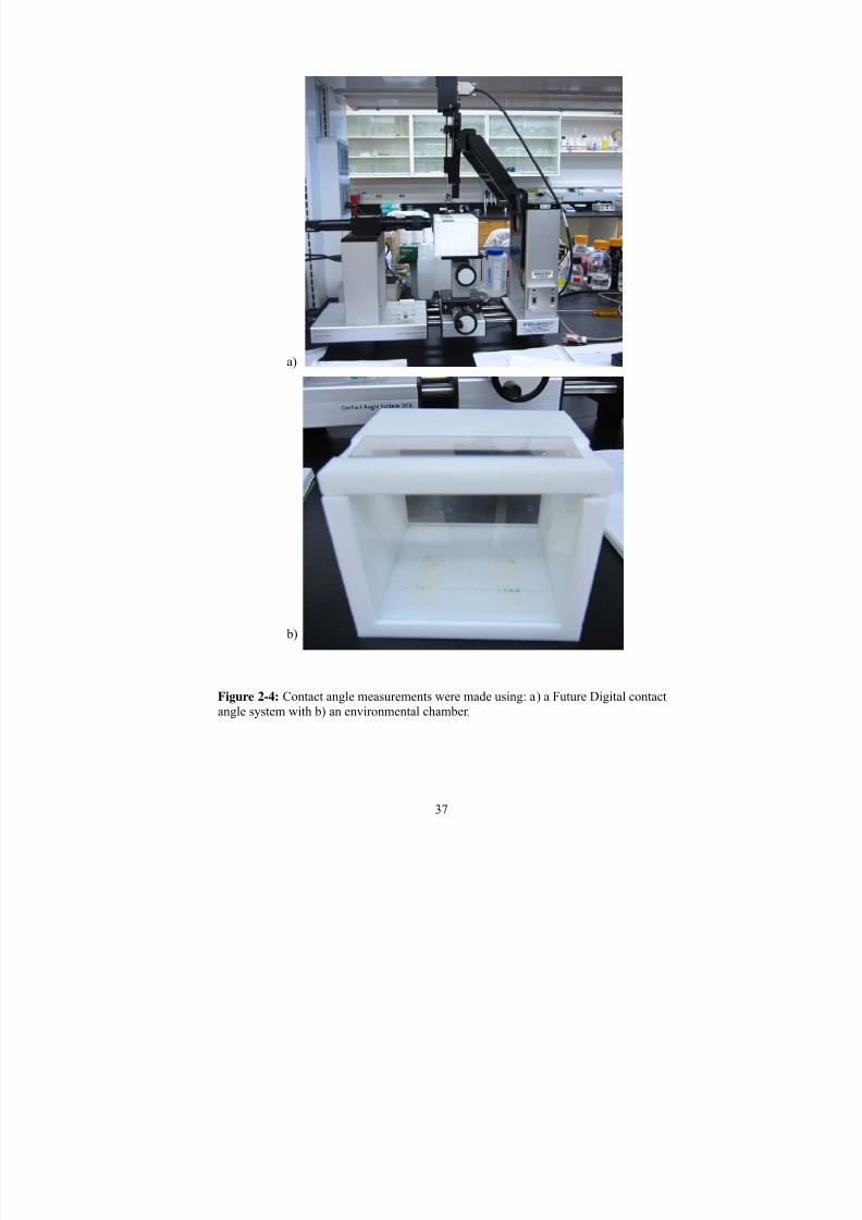
7/27/2019 Atomic Force Microscopy Method Development for Surface Energy Analysis
http://slidepdf.com/reader/full/atomic-force-microscopy-method-development-for-surface-energy-analysis 59/365
37
Figure 2-4: Contact angle measurements were made using: a) a Future Digital contactangle system with b) an environmental chamber .
a)
b)
7/27/2019 Atomic Force Microscopy Method Development for Surface Energy Analysis
http://slidepdf.com/reader/full/atomic-force-microscopy-method-development-for-surface-energy-analysis 60/365
38
Figure 2-5: A screen shot of a sessile drop of a liquid on a solid. The fitting is doneusing the contact angle system software.

7/27/2019 Atomic Force Microscopy Method Development for Surface Energy Analysis
http://slidepdf.com/reader/full/atomic-force-microscopy-method-development-for-surface-energy-analysis 61/365
39
2.5 Contact Angle Results and Evaluation of Indirect Models on Inert Surfaces
The results in this section were necessary to establish a baseline of solid-vapor and solid-
liquid surface energy for reference standards. The results obtained from AFM
measurements presented in Chapter 5 will be compared to the results in this section. This
will help evaluate the AFM’s capabilities and/or limitations.
2.5.1 Static contact angle measurements
The average contact angles for mica and graphite are summarized in Table 2-2. Mica, a
hydrophilic surface, was wetted most significantly with water and least significantly with
diiodomethane,
θdiiodomethane > θethylene glycol > θwater
Water’s polar or AB component was stronger than the other liquids used, illustrating
mica’s hydrophilicity. Ethylene glycol also has a polar/AB component, but the
dispersive/LW component was stronger and thus, the spreading of the droplet is less
compared to water. Diiodomethane only has a dispersive/LW component so the contact
angle was expected to be largest. In summary, the spreadability order on mica was:
Swater > Sethylene glycol > Sdiiodomethane
where S is the spreading of a liquid across the surface. The term gives a different order
than contact angle because spreadability was controlled by all the interfacial properties of
the surface and liquid used in the study. Thus, with a hydrophilic surface, spreading of
water was stronger and the contact angle was small.

7/27/2019 Atomic Force Microscopy Method Development for Surface Energy Analysis
http://slidepdf.com/reader/full/atomic-force-microscopy-method-development-for-surface-energy-analysis 62/365
40
Graphite, a nonpolar surface, has the strongest interaction with diiodomethane and the
least interaction with water.
θwater > θformamide > θdiiodomethane
The weak interaction with water confirms the surface hydrophobicity, and the strong
interaction with diiodomethane confirms that the LW forces on the surface of graphite
were strongest. The interaction with formamide was stronger than water because the
dispersive/LW was larger and the polar/AB component was smaller. Therefore, the order
of spreadability on graphite is
Sdiiodomethane > Sformamide > Swater
The reason ethylene glycol was used on mica and not on graphite was because the contact
angle of graphite-ethylene glycol was similar to the water-diiodomethane angle, which
could have affected the surface energy determination. The reason formamide was not
used on mica was because the spreading was similar to that of water, leading to an
inaccurate fitting with the surface energy models. Many of the indirect models are
criticized for dependence on the liquids used. Therefore, to have three independent and
different interactions, formamide was used with graphite and ethylene glycol was used
with mica.
The ten contact angle measurements from each liquid were used to determine ten solid-
vapor surface energies. The average and standard deviation of these values for both mica
and graphite were determined using the three indirect models previously discussed. The
values are shown in Table 2-3.

7/27/2019 Atomic Force Microscopy Method Development for Surface Energy Analysis
http://slidepdf.com/reader/full/atomic-force-microscopy-method-development-for-surface-energy-analysis 63/365
41
Table 2-2: Average sessile drop contact angles on the surfaces of mica and graphite
Mica
(θ)
Graphite
(θ)
Diiodomethane 41. 0 ± 2.9 37.8 ± 1.4
Ethylene Glycol 23.1 ± 1.2 NA
Formamide NA 60.9 ± 2.4
Water 10.0 ± 2.4 80.6 ± 3.6
Standard deviations were determined from an n=10.

7/27/2019 Atomic Force Microscopy Method Development for Surface Energy Analysis
http://slidepdf.com/reader/full/atomic-force-microscopy-method-development-for-surface-energy-analysis 64/365
42
Table 2-3: Average solid-vapor surface energy for mica and graphite calculated usingvarious indirect models
Van Oss – Chaudhury - Good
γsv γsv
LW
γsv
AB
γsv
-
γsv
+
Mica
41.3 ± 2.7 39.8 ± 2.3 1.5 ± 0.7 72.6 ± 1.5 9.3E-03 ±7.9E-03
Graphite 42.7 ± 2.6 41.5 ± 1.4 1.2 ± 1.3 7.2 ± 3.7 0.1 ± 0.1
OWRK Neumann
γsv γsvd γsv
p γsv
Mica 65.2 ± 0.3 29.7 ± 1.2 35.5 ± 1.2 57.0 ± 0.4
Graphite 40.3 ± 0.7 37.0 ± 1.7 3.3 ± 1.7 36.8 ± 1.1
Standard deviations were determined from an n=10.

7/27/2019 Atomic Force Microscopy Method Development for Surface Energy Analysis
http://slidepdf.com/reader/full/atomic-force-microscopy-method-development-for-surface-energy-analysis 65/365
43
The solid-vapor surface energy range for mica is 41.3 to 65.2 mJ/m2. The lower value
compares to the literature value 43 mJ/m2 because the report from the literature used the
van Oss-Chaudhury-Good model to determine the solid-vapor surface energy.[27] This
model evaluates surface energy based on LW and AB components discussed in the
previous section. Though the overall γAB is small compared to the γLW component, the γ-
is significant. This means that mica’s surface was extremely electron donating. A
similar observation was made with the OWRK model. The polar component in this
model was 35.5 mJ/m2 and was actually larger than the dispersive component. Etzler
believes γ p
is covered in the γLW
component, referring to dipole-dipole interactions.
Thus, the strong mica-water interaction could be explained by the large polar surface
energy component from the OWRK model and a large electron donating surface energy
component by the van Oss model. Even though the two models are not in agreement
with the total solid-vapor surface energy, it was clear mica will have a stronger
interaction with liquids whose characteristics are similar to water and ethylene glycol. As
mentioned previously, no statistical mechanical insight can be gained from the Neumann
model, but the average γsv was found to be between the other models, making it difficult
to determine a single true value for the solid-vapor surface energy of mica.
The solid vapor surface energy range for graphite was 36.8 to 42.7 mJ/m2. The higher
value was obtained using the van Oss-Chaudhury-Good. The value reported in the
literature was 46 mJ/m2, determined using the OWRK model. There was better
agreement between indirect models when evaluating the average solid-vapor surface
energy of graphite instead of mica. The OWRK and van Oss-Chaudhury-Good model
show that the polar/acid-base components respectively were small for graphite. Small

7/27/2019 Atomic Force Microscopy Method Development for Surface Energy Analysis
http://slidepdf.com/reader/full/atomic-force-microscopy-method-development-for-surface-energy-analysis 66/365
44
values were calculated when the van Oss-Chaudhury-Good model was broken into the
electron donating-accepting components. These results bring up a point of contention
with this model. The total γAB component for both mica and graphite was small;
however, the γ- for mica was much larger in comparison, though not reflected in the
overall term because of a small γ+. At first glance, it would seem the dispersive/LW
interactions were dominant on the surface of both mica and graphite. However, the
strong mica-water and mica-ethylene glycol interaction indicated another force must be
contributing to the surface energetics. Lastly, the Neumann model was used to calculate
γsv. The Neumann value was comparable to the γd term in the OWRK model.
Neumann’s modification to the geometric mean was made in order to prevent
overestimation of the surface energy. Calculation of the γLW of van Oss-Chaudhury-
Good model was solely based on the geometric mean, and therefore, it is larger than
Neumann’s γsv.
The mica and graphite solid-vapor surface energy results illustrate how each model
evaluated van der Waals and polar/AB forces differently. Since there was no agreement
in the solid-vapor surface energies on mica, these models might be better suited for
analyzing surfaces dominated by van der Waals forces. Each model relies on the
foundation of the geometric mean which evaluates van der Waals interactions: London
dispersion, Debye, and Keesom interactions. These models have incorporated the polar
interaction, the acid-base interaction, or a corrections factor, but these components were
not comparable with mica. For this reason, the AFM may be a more attractive tool for
studying surface energy on a variety of surfaces.

7/27/2019 Atomic Force Microscopy Method Development for Surface Energy Analysis
http://slidepdf.com/reader/full/atomic-force-microscopy-method-development-for-surface-energy-analysis 67/365
45
Now that the solid-vapor surface energy has been calculated, the solid-liquid surface
energy can be calculated from Young’s Equation and contact angle data. Results are
shown in Table 2-4.
As expected, the range of solid-liquid surface energies for mica was very large because of
the large difference in the solid-vapor surface energies. As with solid-vapor surface
energies, the solid-liquid surface energy values for all of the liquids makes it difficult to
identify a so called “true” value. However, the graphite data was more comparable
because of the similarities with the solid-vapor surface energy. Figure 2-6 shows the
range of mica and graphite solid-liquid surface energy using histograms. The Y axis was
the frequency plotted against the solid-liquid surface energy. The range of solid-liquid
surface energy for graphite-diiodomethane was -3 to 1 mJ/m2 (shown in blue). The
negative numbers for graphite have no physical meaning and were a result of limitations
from the indirect models. Young’s equation attempts to balance the forces among the
three phases; therefore, the solid-liquid surface energy may result in negative numbers
when γsv is less than γlv cos(θ). The ranges of solid-liquid surface energy for graphite-
formamide (9-14 mJ/m2) and graphite-water (25-30 mJ/m2) were consistent with the
results of the contact angles. The lowest solid-liquid surface energy was graphite-
diiodomethane because there was a stronger interaction (smaller contact angle). The
largest solid-liquid surface energy was graphite-water because there was a weaker
interaction (large contact angle).

7/27/2019 Atomic Force Microscopy Method Development for Surface Energy Analysis
http://slidepdf.com/reader/full/atomic-force-microscopy-method-development-for-surface-energy-analysis 68/365
46
Table 2-4: Average solid-liquid surface energies for mica and graphite calculated fromsolid-vapor surface energies of various indirect models.
Mica Graphite
OWRK
Van Oss-
Chaudhury-Good Neumann OWRK
Van Oss-
Chaudhury-Good Neumann
γsl
(mJ/m2)
Diiodomethane 26.9 ± 1.5 0.8 ± 0.2 18.7 ± 1.7 0.7 ± 0.9 0.6 ± 0.1 -3.3 ± 1.6
EthyleneGlycol
21.1 ± 0.4 -3.6 ± 1.7 12.8 ± 0.3 NA
Formamide NA 12.6 ± 2.2 13.7 ± 2.8 8.7 ± 1.9
Water -6.4 ± 0.5 -31.1 ± 2.3 -14.7 ± 0.6 29.0 ± 4.2 30.0 ± 3.9 25.0 ± 3.5
Standard deviations were determined from an n=10.

7/27/2019 Atomic Force Microscopy Method Development for Surface Energy Analysis
http://slidepdf.com/reader/full/atomic-force-microscopy-method-development-for-surface-energy-analysis 69/365
47
Figure 2-6: Solid-liquid surface energies of a) graphite and b) mica for the liquids usedto measure contact angles and determine solid-vapor surface energy.
0
2
4
6
8
10
12
1416
-34 -22 -10 2 14 26 38
Surface Energy (mJ/m2)
DiiodomethaneEthylene Glycol
Water
b)
0
2
4
68
10
12
14
16
-34 -22 -10 2 14 26 38
Surface Energy (mJ/m2)
Diiodomethane
Formamide
Water
a)
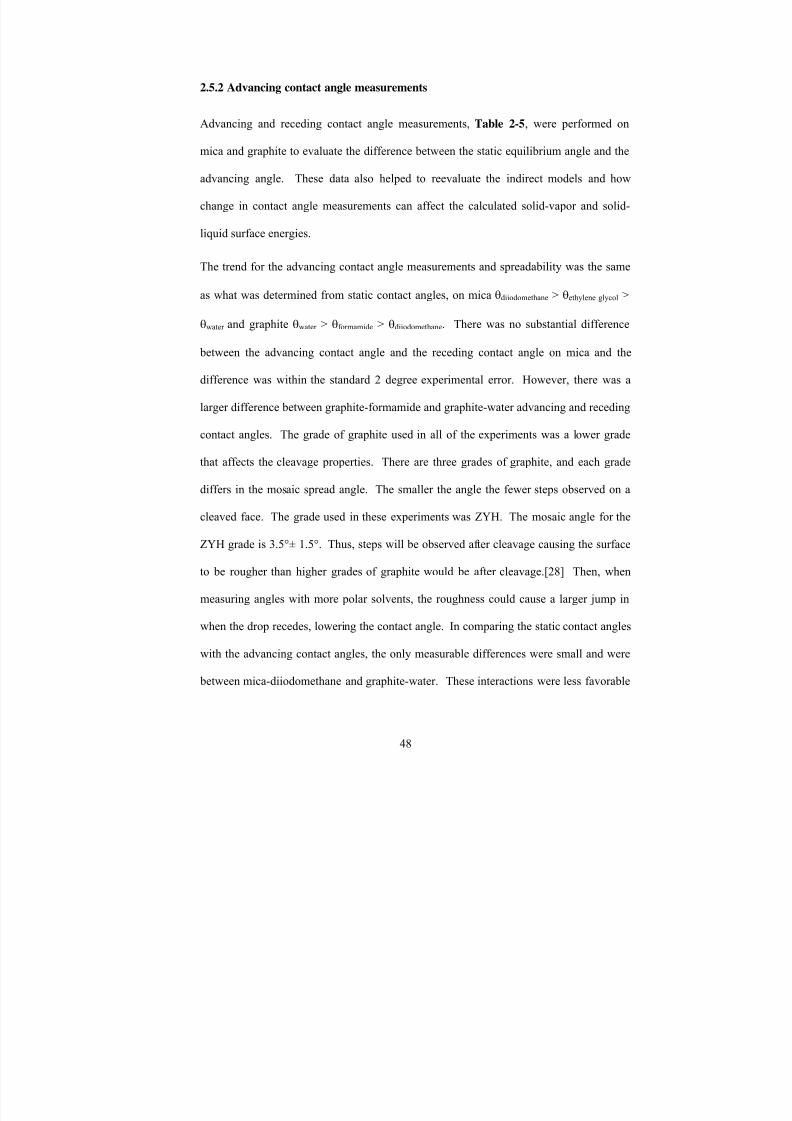
7/27/2019 Atomic Force Microscopy Method Development for Surface Energy Analysis
http://slidepdf.com/reader/full/atomic-force-microscopy-method-development-for-surface-energy-analysis 70/365
48
2.5.2 Advancing contact angle measurements
Advancing and receding contact angle measurements, Table 2-5, were performed on
mica and graphite to evaluate the difference between the static equilibrium angle and the
advancing angle. These data also helped to reevaluate the indirect models and how
change in contact angle measurements can affect the calculated solid-vapor and solid-
liquid surface energies.
The trend for the advancing contact angle measurements and spreadability was the same
as what was determined from static contact angles, on mica θdiiodomethane > θethylene glycol >
θwater and graphite θwater > θformamide > θdiiodomethane. There was no substantial difference
between the advancing contact angle and the receding contact angle on mica and the
difference was within the standard 2 degree experimental error. However, there was a
larger difference between graphite-formamide and graphite-water advancing and receding
contact angles. The grade of graphite used in all of the experiments was a lower grade
that affects the cleavage properties. There are three grades of graphite, and each grade
differs in the mosaic spread angle. The smaller the angle the fewer steps observed on a
cleaved face. The grade used in these experiments was ZYH. The mosaic angle for the
ZYH grade is 3.5°± 1.5°. Thus, steps will be observed after cleavage causing the surface
to be rougher than higher grades of graphite would be after cleavage.[28] Then, when
measuring angles with more polar solvents, the roughness could cause a larger jump in
when the drop recedes, lowering the contact angle. In comparing the static contact angles
with the advancing contact angles, the only measurable differences were small and were
between mica-diiodomethane and graphite-water. These interactions were less favorable

7/27/2019 Atomic Force Microscopy Method Development for Surface Energy Analysis
http://slidepdf.com/reader/full/atomic-force-microscopy-method-development-for-surface-energy-analysis 71/365
49
than mica-water and graphite-diiodomethane; therefore, a three or four degree difference
was not uncommon. Since there were few differences between the static and advancing
contact angles, the average solid-vapor and solid-liquid energies should also be
comparable. The advancing solid-vapor and solid-liquid surface energies are shown in
Table 2-6 and Table 2-7. Reviewing Table 2-3 and Table 2-4, the solid-vapor and
solid-liquid surface energies calculated from static contact angles, prove the assumption
of comparability to be true. The small difference in mica-diiodomethane and graphite-
water did not change the overall solid-vapor surface energy and did not change the
components. There were still major differences in the three indirect models when
evaluating γsv for mica, but it remains easier to compare the solid-vapor surface energy of
graphite among the three models.

7/27/2019 Atomic Force Microscopy Method Development for Surface Energy Analysis
http://slidepdf.com/reader/full/atomic-force-microscopy-method-development-for-surface-energy-analysis 72/365
50
Table 2-5: Average advancing and receding contact angles measured on the surfaces of mica and graphite
Mica Graphite
Advancing
(θ)
Receding
(θ)
Advancing
(θ)
Receding
(θ)
Diiodomethane 46.1 ± 0.8 44.2 ± 1.1 37.9 ± 2.3 36.4 ± 1.4
Ethylene Glycol 23.7 ± 3.7 23.2 ± 3.6 NA
Formamide NA 58.5 ± 3.2 54.7 ± 3.6
Water 11.1 ± 2.4 10.3 ± 2.1 83.0 ± 2.8 76.0 ± 3.7
Standard deviations were determined from an n=10.
7/27/2019 Atomic Force Microscopy Method Development for Surface Energy Analysis
http://slidepdf.com/reader/full/atomic-force-microscopy-method-development-for-surface-energy-analysis 73/365
51
Table 2-6: Average solid-vapor surface energies for mica and graphite calculated fromadvancing contact angles and various indirect models
Van Oss – Chaudhury - Good
γsv γsvLW γsv
AB γsv- γsv
+
Mica 42.8 ± 3.6 38.6 ± 2.4 4.2 ± 1.6 73.2 ± 1.76.9E-02 ±5.6E-02
Graphite 42.7 ± 1.3 41.2 ± 1.3 1.5 ± 0.6 4.3 ± 2.6 0.3 ± 0.3
OWRK Neumann
γsv γsv
d
γsv
p
γsv Mica 64.9 ± 1.2 29.7 ± 1.0 37.0 ± 0.6 57.0 ± 0.4
Graphite 41.3 ± 1.1 38.8 ± 1.6 2.5 ± 0.9 36.5 ± 0.9
Standard deviations were determined from an n=10.

7/27/2019 Atomic Force Microscopy Method Development for Surface Energy Analysis
http://slidepdf.com/reader/full/atomic-force-microscopy-method-development-for-surface-energy-analysis 74/365
52
Table 2-7: Average solid-liquid surface energies calculated from advancing contact angledata and solid-vapor surface energy from various indirect models.
Mica Graphite
OWRK Van Oss-
Chaudhury-Good
Neumann OWRK Van Oss-
Chaudhury-Good
Neumann
γsl
(mJ/m2)
Diiodomethane 29.7 ± 0.8 1.2 ± 0.1 21.7 ± 0.7 1.4 ± 1.1 0.6 ± 0.1 -3.5 ± 1.4
EthyleneGlycol 21.1 ± 1.0 -3.3 ± 0.9 13.1 ± 1.4 NA
Formamide NA 11.2 ± 2.4 11.9 ± 2.6 6.3 ± 2.6
Water -6.5 ± 0.7 -30.8 ± 1.8 -14.4 ± 0.8 32.7 ± 3.9 33.3 ± 3.8 27.7 ± 2.8
Standard deviations were determined from an n=10.

7/27/2019 Atomic Force Microscopy Method Development for Surface Energy Analysis
http://slidepdf.com/reader/full/atomic-force-microscopy-method-development-for-surface-energy-analysis 75/365
53
The purpose of these experiments was to evaluate the contact angle hysteresis. Since
graphite and mica are relatively ideal surfaces, there was no substantial difference in
advancing and receding contact angles. Also, the advancing angles were comparable to
the static equilibrium angles. Therefore, the advancing and receding evaluation did not
change the results of the calculated surface energies. The solid-vapor and solid-liquid
surface energy range for mica was still large, and the results for graphite were
comparable between the models. The negative numbers were still seen with mica-water
and graphite-diiodomethane, illustrating the dependence of the indirect models.
2.5.3 Static contact angle measurements with hygroscopic liquids
Evaluation of the effect hygroscopic liquids have on contact angle measurements was the
final study performed. The two hygroscopic solvents used in these studies were ethylene
glycol and formamide.
Table 2-8 shows the water content of the liquids after drying. A typical plot for contact
angle measurements is shown in Figure 2-7a. This plot differs from the plots obtained
after the liquids were hydrated, Figure 2-7b. Instead of reaching an equilibrium which is
obtained after the droplet has finished spreading, the contact angle continues to get larger.
After waiting 240 seconds, the same droplet was recorded for 3 minutes, and a possible
equilibrium angle was found Figure 2-7c. These angles were recorded and an average
was determined for dry, 0.5, 1.0 and 5.0% w/w formamide-water on graphite and
ethylene glycol-water on mica, Table 2-9. It was hypothesized that water in ethylene
glycol would cause a decrease in contact angle from the dried angle because water has a
strong interaction with mica; however, an increase was observed. The difference in the
concentration of water present, between 0.5% and 5.0%, did not affect the angle

7/27/2019 Atomic Force Microscopy Method Development for Surface Energy Analysis
http://slidepdf.com/reader/full/atomic-force-microscopy-method-development-for-surface-energy-analysis 76/365
54
measured since the angles are very similar. For formamide on graphite, an increase in
water should increase the contact angles because water interacts weakly with graphite.
This was observed when measuring the contact angles with formamide containing water.
The standard deviations between the different concentrations of formamide-water were
larger than what is seen with pure liquids. Therefore, it is important to use pure liquids
when measuring contact angles in order to find the “true” interaction between that liquid
and the sample. The measured angles from the dried liquids were used in Section 2.5 to
calculate the solid-vapor and solid liquid surface energies.
Since diiodomethane was the other solvent used in the contact angle experiments, the
water content was evaluated using KF. The initial value was as low as the values for
dried ethylene glycol and dried formamide. Hydration of diiodomethane was attempted.
Excess water was added to a vial of diiodomethane and rotated continuously for three
days. Each day the water content was tested. The water content did not increase from
the initial value shown in Table 2-8.

7/27/2019 Atomic Force Microscopy Method Development for Surface Energy Analysis
http://slidepdf.com/reader/full/atomic-force-microscopy-method-development-for-surface-energy-analysis 77/365
55
Table 2-8: Water content of liquids used in contact angle measurements after being driedand the initial amount of water for diiodomethane measured directly from the bottle.
Solvent Water Content% w/w
Dried Formamide 0.04
Dried Ethylene Glycol 0.03
Diiodomethane 0.01

7/27/2019 Atomic Force Microscopy Method Development for Surface Energy Analysis
http://slidepdf.com/reader/full/atomic-force-microscopy-method-development-for-surface-energy-analysis 78/365
56
Table 2-9: Contact angles measured on mica and graphite with dried and rehydratedethylene glycol and formamide respectively
Mica Graphite
Ethylene Glycol (θ) Formamide (θ)
Dried 23.1 ± 1.2 Dried 60.9 ± 2.4
0.5 % w/w water 30.9 ± 1.3 0.5 % w/w water 65.6 ± 4.5
1.0% w/w water 32.2 ± 2.3 1.0% w/w water 62.4 ± 3.8
5.0% w/w water 30.5 ± 1.3 5.0% w/w water 64.3 ± 4.1
Standard deviations were determined from an n=10.

7/27/2019 Atomic Force Microscopy Method Development for Surface Energy Analysis
http://slidepdf.com/reader/full/atomic-force-microscopy-method-development-for-surface-energy-analysis 79/365
57
Figure 2-7: Contact angle measurements shown over time for a) a dried solvent, b) ahydrated solvent, and c) the possible equilibrium angle of the hydrated solvent 3 minutesafter the initial recording
0
5
10
15
20
25
30
35
0 34 67 100 133 166 200 233
Time (sec)
C o
n t a c t A n g l e (θ
)
0
1
2
3
4
5
B a s e l i n e D i a m e t e r
( m m )
CA(R)
CA(M)
CA(L)
BD
0
5
10
15
20
25
30
35
0 26 52 78 103 129 155 181 206 232Time (sec)
C o n t a c t A n g l e (θ
)
0
1
2
3
4
5
B a s e l i n e D i a m e t e r
( m m )
0
5
10
15
20
25
30
35
0 26 52 78 103 129 155 181 206 232
Time (sec)
C o n t a c t A n g l e (θ
)
0
1
2
3
4
5
B a s e l i n e D i a m e t e r
( m m )
a)
b)
c)

7/27/2019 Atomic Force Microscopy Method Development for Surface Energy Analysis
http://slidepdf.com/reader/full/atomic-force-microscopy-method-development-for-surface-energy-analysis 80/365
58
2.6 Contact Angle Summary
Young’s equation defines the forces at the three-phase boundary of a liquid droplet on a
surface. In order to determine the solid-vapor surface energy from Young’s equation,
indirect models were developed. These equations are part of the limitations of contact
angle measurements. The indirect models did not agree in the process of defining
independent interactions (van Oss et al and OWRK) or if the division of components is
the best approach (Neumann). Since there were theoretical differences in the models, the
overall surface energy values derived by these models could not be compared when
measured for mica, a hydrophilic material. However, the surface energies determined for
graphite using all three models were comparable. Graphite was dominated by dispersive
energies, and since the models are mathematically based on the geometric mean, which
defines the London dispersive, Debye, and Keesom forces, the surface energy values of
graphite were expected to be comparable.
One limitation from the contact angle measurements was the difficulty or inability to
draw conclusions from data without scientific meaning. Negative solid-liquid surface
energies were calculated for both mica and graphite. These values do not have a physical
meaning and will be difficult to compare with AFM results.
The other challenges with contact angle measurements were the experimental
methodologies. Controlling the humidity is difficult because of a restricted number of
useful solvents to attain an equilibrium contact angle. Water and other solvents that
evaporate rapidly require a saturated environmental chamber to measure the angle. Only
pure liquids can be used, and if the liquid interacts with the surface causing deformation,
measuring the true contact angle is difficult.
7/27/2019 Atomic Force Microscopy Method Development for Surface Energy Analysis
http://slidepdf.com/reader/full/atomic-force-microscopy-method-development-for-surface-energy-analysis 81/365
59
All of these disadvantages made investigating the AFM a necessity. Although contact
angle measurements are still used to investigate surface energetics, the shortcomings
prompted the need to evaluate the performance of other techniques. Therefore, the
results in this chapter will provide a baseline for surface energy values with mica and
graphite. The AFM was then used to evaluate the surface energy on mica and graphite.
To determine the AFM’s capability, the surface energy results will be compared to the
contact angle results in this chapter.
Copyright © Clare Aubrey Medendorp 2011

7/27/2019 Atomic Force Microscopy Method Development for Surface Energy Analysis
http://slidepdf.com/reader/full/atomic-force-microscopy-method-development-for-surface-energy-analysis 82/365
60
Chapter 3 – Atomic Force Microscopy
The focus of this chapter is to review the operations of atomic force microscopy (AFM)
and how that instrument can be used to measure forces. The methodology of
characterizing AFM tip properties, measuring forces, and using statistical analysis is
presented. The overarching goal is to establish a robust experimental method to obtain
repeatable measurements that can be used to evaluate surface energy.
3.1 Atomic Force Microscopy Introduction
Scanning probe microscopes are unique in that they can provide three-dimensional real
space images and can allow spatially localized measurements of structure and
properties.[29] The scanning probe microscopes create images with a very fine probe tip
which scans over the sample instead of the typical visual observations. The atomic force
microscope (AFM), depicted in Figure 3-1, was invented by Binning et al [30] in 1986
and belongs to the series of scanning probe microscopes. The AFM, since its discovery,
has become an important tool for imaging topography and measuring forces of sample
surfaces as it is not limited to conducting samples.[31] The AFM is comprised of three
major components: the tip, the piezoelectric crystal, and the detection mechanism.
The stylus, or tip, is the key piece of the AFM that scans and interacts with the sample
surface. The basic tip is micro-fabricated, extremely sharp, and mounted on the end of a
cantilever. The cantilever is bonded to a glass chip that is easily mounted in the sample
holders. The interaction of the tip with the sample is recorded through movement of the
cantilever. The cantilever typically has a low force constant allowing for precise control
of the force between the tip and sample.[31] The force constant of the cantilever will be

7/27/2019 Atomic Force Microscopy Method Development for Surface Energy Analysis
http://slidepdf.com/reader/full/atomic-force-microscopy-method-development-for-surface-energy-analysis 83/365
61
discussed further in Section 3.3. Different tips have developed as imaging techniques
advance. Therefore, the silicon and silicon nitride tips are not the only tips commercially
available. AFM tips can also be modified chemically or “naked” cantilevers can be
purchased to tailor the tip to a specific interaction of interest.
The critical feature that allows the three dimensional scanning of the tip is the
piezoelectric crystal. The AFM utilizes the reverse piezoelectric effect. When a potential
difference is applied to opposite faces of the crystal, it changes shape. The piezoelectric
tube is arranged with five electrodes: z is in the middle, –x and +x are across from each,
and –y and +y are also opposite each other, Figure 3-2. When a bias voltage is applied
between the inner and the outer electrodes, the tube expands or contracts and moves in
the z direction. If voltage is applied to one of the outer electrodes, the tube will bend and
then move in either the x or y directions. When the tip is in contact with the surface, the
exact movement of the cantilever is known, because the exact movement of the
piezocrystal is known.[31]

7/27/2019 Atomic Force Microscopy Method Development for Surface Energy Analysis
http://slidepdf.com/reader/full/atomic-force-microscopy-method-development-for-surface-energy-analysis 84/365
62
Figure 3-1: Schematic of atomic force microscope with key features.
Piezoelectric
Cylinder/Scanner
Cantilever
with Tip
Laser Photodetector
A B
C D
Piezoelectric
Cylinder/Scanner
Cantilever
with Tip
Laser Photodetector
A B
C D

7/27/2019 Atomic Force Microscopy Method Development for Surface Energy Analysis
http://slidepdf.com/reader/full/atomic-force-microscopy-method-development-for-surface-energy-analysis 85/365
63
The most common detection of the cantilever movement is the optical lever technique. A
beam from a laser diode is focused onto the end of the cantilever and the beam is
reflected into a photodetector. The sensitivity of the change in cantilever movement is
derived from the large distance between the cantilever and the photodiiode. Most
photodetectors are simple photodiodes. A photodiode is a semiconductor device which
turns the laser into an electrical signal. The photodiode is split into four sections, as
shown in Figure 3-1, allowing for lateral and torsional motion of the cantilever to be
detected.[31] The cantilever’s lateral deflection is measured by monitoring the laser’s
change in position on the photodetector. The vertical signal is (A + B) − (C + D), whilethe (A + C) − (B + D) signal responds to friction due to torsion of the cantilever,
providing lateral force information, Figure 3-1.[32, 33]

7/27/2019 Atomic Force Microscopy Method Development for Surface Energy Analysis
http://slidepdf.com/reader/full/atomic-force-microscopy-method-development-for-surface-energy-analysis 86/365
64
Figure 3-2: The piezo scanner moves the sample in three direction: x, y, and zmovements. The top view schematic a) shows the five electrodes needed to achieve this,and b) is a 3D view to help visualize the z or vertical movement.
z
+y
-y
-x +xz
+y
-y
-x +x
Z
XX
Y

7/27/2019 Atomic Force Microscopy Method Development for Surface Energy Analysis
http://slidepdf.com/reader/full/atomic-force-microscopy-method-development-for-surface-energy-analysis 87/365
7/27/2019 Atomic Force Microscopy Method Development for Surface Energy Analysis
http://slidepdf.com/reader/full/atomic-force-microscopy-method-development-for-surface-energy-analysis 88/365
66
reduction in time on the surface. Less drag occurs, which enhances the resolution of a
topographical image. Another benefit is delicate samples can be imaged without damage
or severe image distortion. In addition, capillary and lateral (side to side) forces can be
lessened or avoided with less time on the sample.[31] During tapping mode trapped
electric charges on the surfaces are also eliminated. Tapping mode can be operated in air
and in liquid. As previously stated, the goal of this work is to evaluate the AFM’s ability
in studying surface energy. Therefore, tapping mode cannot be used because this mode
does not measure forces of adhesion.
The easiest and most widely used mode of the AFM is contact mode. In this mode, the
AFM tip is in intimate repulsive contact with the surface of the sample. The scanner
traces over the sample causing the cantilever to bend because of changes in topography or
the probe-sample forces. There are two variations of the contact mode: constant-force
and variable-deflection mode. In constant-force mode, the cantilever deflection is kept
constant with a feedback loop that adjusts the height of the sample such that a constant
deflection is maintained. The height is varied by extending or retracting the piezo along
the z axis. The other mode is variable-deflection mode. In this mode the height is held
constant and cantilever deflection is monitored. One disadvantage of contact mode is the
effect capillary forces can have on the image and force measurements. However,
controlling humidity and using liquids can reduce or eliminate the effect of capillary
forces.[31]

7/27/2019 Atomic Force Microscopy Method Development for Surface Energy Analysis
http://slidepdf.com/reader/full/atomic-force-microscopy-method-development-for-surface-energy-analysis 89/365
67
Figure 3-3: Typical AFM force curve.

7/27/2019 Atomic Force Microscopy Method Development for Surface Energy Analysis
http://slidepdf.com/reader/full/atomic-force-microscopy-method-development-for-surface-energy-analysis 90/365
68
The other prominent imaging technique of the AFM used for this study is force-imaging.
During contact mode scanning, the force of adhesion between the tip and the sample is
evaluated by measuring the deflection of the cantilever. The forces can be derived from
the force curve output by AFM, as shown in Figure 3-3. In a typical force measurement,
two plots are obtained as the piezocrystal is extended and retracted. At the start of
extension, marked by point 1 in Figure 3-3, there is a large distance between the tip and
the sample. As the voltage is applied, the piezocrystal starts to extend, the distance
decreases, and the force acting on the tip exceeds the stiffness of the cantilever. This
causes the tip to jump into contact with the sample surface, points 2-4. Deflections aredominated by mutual repulsions, causing the piezocrystal to begin retracting, separating
the tip from the sample. However, separation does not occur until the bent cantilever
overcomes the adhesion forces, pulling off sharply to a non-contact position, points 4-7 in
Figure 3-3.[33] Initially, the output is expressed as cantilever deflection (in terms of
volts on the photo diode) vs. piezocrystal displacement, since the only known is the
movement of the piezo, Z distance. This plot can be translated into a force vs. distance
plot based on Hooke’s Law (F=-k*Δx) where Δx is the displacement measured by the
AFM and k is the spring constant.[32] The methods for determining spring constant will
be discussed in the next section. To determine the deflection (Δx) from the force curves,
SPIP software was used. However, the theoretical determination of Δx is shown in
Section 3.6.3. With proper calibration, these two parameters, and therefore, F, can be
obtained with good accuracy.

7/27/2019 Atomic Force Microscopy Method Development for Surface Energy Analysis
http://slidepdf.com/reader/full/atomic-force-microscopy-method-development-for-surface-energy-analysis 91/365
69
3.3 AFM Tip Characterization
The cantilever is a key element of the AFM. Cantilevers can be either rectangular or
triangular. The triangular cantilevers typically experience less torsional force, which is
important when measuring vertical displacement. The mechanical properties of
cantilevers are characterized by the spring constant and resonance frequency and are
mainly responsible for the AFM’s performance. Cantilevers are typically made from
silicon or silicon nitride. The top side is coated with gold or aluminum to increase
reflectivity of the laser into the photodiode. This section details the evaluation of the
spring constant and the tip radius. In Chapter 4, the importance of the tip radius is in
determining surface energy for AFM force measurements will be discussed.
3.3.1 Calibration of spring constants
A cantilever should have high sensitivity, and this is achieved with a low spring
constant.[29] The spring constant describes the stiffness of the cantilever in force per
unit length and must be determined to calculate the force.[31, 32] There have been
several methods established to measure the spring constant of a cantilever. Added mass
and thermal methods have been the most popular, but a geometric analysis was the initial
technique using[41]
3
3c
4L
Ewtk = 3.1
where k is the spring constant, E is the Young’s modulus, tc is the thickness, w is the
width, and L is the length. Using a scanning electron microscope (SEM), the cantilever’s
width and length can be measured. It is much more difficult to measure the thickness and
the Young’s modulus: therefore, manufacturers will report an average for these values.

7/27/2019 Atomic Force Microscopy Method Development for Surface Energy Analysis
http://slidepdf.com/reader/full/atomic-force-microscopy-method-development-for-surface-energy-analysis 92/365
70
Consequently, the geometric method is not preferred because the thickness and Young’s
modulus of the individual cantilevers vary. It has been shown that cantilevers are not
perfectly homogeneous and since thickness in Equation 3.1 is to the third power, a small
difference in thickness can lead to a significant change in spring constant. The Young’s
modulus of a thin layer can deviate from the bulk material and Khan has shown that a
silicon nitride sample 800 nm thick had a Young’s modulus of 280 GPa rather than the
reported 146 GPa.[42] The thickness of the native oxide layer and the gold layer are both
unknown. These unknowns add to the mass of the cantilever which influences the
resonance frequency and the spring constant.[32]
3.3.1.1 Added mass method
A more prevalent method, regarded as the “gold standard” to measuring the spring
constant, is the added mass method developed by Cleveland et al.[43] The technique for
this method relies on measuring the resonance frequency of the cantilever before (ν0) and
after (ν1), the addition of a tungsten sphere behind the tip. By adding a mass M to the
cantilever the resonant frequency becomes:
m M
k v
+=
π 2
1 3.2
where m is the mass of the cantilever. After the sphere is added, the equation for the
spring constant becomes:
( )20
21
2 M)2(k
−− −=
vvπ 3.3

7/27/2019 Atomic Force Microscopy Method Development for Surface Energy Analysis
http://slidepdf.com/reader/full/atomic-force-microscopy-method-development-for-surface-energy-analysis 93/365

7/27/2019 Atomic Force Microscopy Method Development for Surface Energy Analysis
http://slidepdf.com/reader/full/atomic-force-microscopy-method-development-for-surface-energy-analysis 94/365
72
P. The integration under the power spectrum equals the mean-square in the time data;
therefore, the estimation of the spring constant is:
PTk Bk = 3.6
This method can be used to measure the spring constant in air and in liquids without
destroying the tip or cantilever. Therefore, this method has become the preferred method
for spring constant determination.

7/27/2019 Atomic Force Microscopy Method Development for Surface Energy Analysis
http://slidepdf.com/reader/full/atomic-force-microscopy-method-development-for-surface-energy-analysis 95/365

7/27/2019 Atomic Force Microscopy Method Development for Surface Energy Analysis
http://slidepdf.com/reader/full/atomic-force-microscopy-method-development-for-surface-energy-analysis 96/365
74
3.3.2 Tip radius measurements
Two methods have been used to measure tip radius. One direct way is capturing an
image with scanning electron microscopy (SEM). The other method utilizes the
information gained in a topography scan with the AFM. The quantity of the tip radius is
not necessary for calculating forces, but in Chapter 4, the importance of tip radius will be
presented.
3.3.2.1 SEM method
The SEM creates an image of the sample surface by scanning it with a high-energy beam
of electrons. From this image the radius of the tip can be determined, Figure 3-5. The
evaluation of the SEM image to determine the tip radius is limited at the nanometer scale.
Due to the electron beam size, focus, charging effects, and beam-sample interaction, the
tip’s edge positions are uncertain at the nanometer level.[45] The tip must also be coated
before imaging to prevent charging of the sample. Dongmo showed the coating can
overestimate the tip radius by about 4 nm.[45] The limitation of the SEM image alsomakes it hard for comparison with the other methods of interest.
3.3.2.2 Blind reconstruction method
Blind reconstruction uses the AFM to scan a specific tip characterizer sample to
determine the shape of the probe. The reconstruction method uses a so called “self-
imaging” technique, meaning the image obtained from a tip scanning the topography of
the sample is then used to estimate that tip’s radius. Each pixel from the image contains
information about the tip geometry and the sample surface. The topography image
reveals the inverted geometry of the end of the tip. First, an upper limit on the size of the
probe is determined from the image because the features of the image are always broader
7/27/2019 Atomic Force Microscopy Method Development for Surface Energy Analysis
http://slidepdf.com/reader/full/atomic-force-microscopy-method-development-for-surface-energy-analysis 97/365
75
than the probe used. The upper limits are based on point of inflection, or maxima on the
topography image. These upper limits are created by the shape of the tip. The
intersection of the two points gives an estimation of the tip. Dongmo illustrated this with
an overlaid image of a trace of what an AFM probe would create on top of an image of
the actual surface.[45] The algorithm developed by Villarrubia for blind reconstruction
extracts the maxima, and by calculating the intersection, the tip radius can be
determined.[46-48]
Since the SEM is a destructive method of measuring the tip radius and the radius is an
important parameter in determining surface energy, a method was needed to constantly
monitor the tip radius. The constant monitoring would also allow users to know when a
tip becomes dull. Dull tips can skew force measurements because they can change the
contact area. The contact area is one parameter that was determined to be crucial in
controlling variability of force measurements.

7/27/2019 Atomic Force Microscopy Method Development for Surface Energy Analysis
http://slidepdf.com/reader/full/atomic-force-microscopy-method-development-for-surface-energy-analysis 98/365
76
Figure 3-5: SEM image of a silicon nitride tip.

7/27/2019 Atomic Force Microscopy Method Development for Surface Energy Analysis
http://slidepdf.com/reader/full/atomic-force-microscopy-method-development-for-surface-energy-analysis 99/365
77
3.4 AFM Scanning Parameters
Thus far the operations of the AFM have been discussed. The objective of this work is to
be able to use the AFM to determine surface energy. Therefore, the force imaging
function of the AFM is going to be used. It was realized that in order to develop a
technique, the probe’s properties, such as tip radius and spring constant, will have to be
evaluated, as will other parameters that can affect the precision and accuracy of the
instrument. Key parameters were identified and evaluated to increase the repeatability of
force measurements at different locations on a sample and with the same tip. The critical
scan parameters that were identified are scan size, scan rate, force applied and contact
area.
3.4.1 Scan size
Following the engagement of the tip with the sample, the next step is to view and
optimize the scan in the advance force mode, shown in Figure 3-6. This mode allows the
user to view the force plot output created by the tip-sample interaction. In this mode, the
scan parameters can be changed to establish control over the tip-sample interaction.
Scan size is affected by the type of AFM scanner that is used. Some common scanners
are E and J with maximum scans size of 10 x 10 μm and 125 x 125 μm respectively.
These various sizes are more important when evaluating topography. For a force curve it
is best to take force measurements in a single spot and then move to other discrete spots
on the sample to gather more force data. There were several reasons for choosing a
proper scan size. First, in some liquids and on rough surfaces, a large scan size can cause
drag and skew the actual tip-sample interaction. Drag typically causes hysteresis, an
offset seen with force curves when the “snap off” or retracting line does not follow the

7/27/2019 Atomic Force Microscopy Method Development for Surface Energy Analysis
http://slidepdf.com/reader/full/atomic-force-microscopy-method-development-for-surface-energy-analysis 100/365
78
same path as the “snap in” or advancing line. When there is hysteresis, it is difficult to
determine the “true” force between the tip and surface, as illustrated in Figure 3-7.
Second, tip diameters range from 80 to 120 nm, so when using a scan area smaller than
the tip, the information gleaned is similar to a moving average and not a discrete
measurement. Lastly, when investigating the forces on rough or heterogeneous samples,
the results over a larger area might be confounding because of the AFM’s sensitivity. It
will be hard to elucidate the range of force resulting from the various chemical moieties,
roughness, or true tip-sample interaction. For these reasons, multiple discrete
measurements were made instead of large area measurements.

7/27/2019 Atomic Force Microscopy Method Development for Surface Energy Analysis
http://slidepdf.com/reader/full/atomic-force-microscopy-method-development-for-surface-energy-analysis 101/365
79
Figure 3-6: Advance force mode controls – At this screen, force calibration settings can be manipulated so that the best force curve may be obtained. This screen is the first steponce the tip is engaged with the surface. From this screen, the start position, scan size,scan rate, and amplitude applied to the Z piezo can be controlled. The setpoint value of
the deflection voltage used in the feedback loop can be adjusted, and the type of trigger threshold can be varied. This force mode is used to adjust the force applied so that thecontact area is reached and maintained. Once the parameters are set and an optimal forcecurve is observed, this mode can be exited and data can be collected.[49]
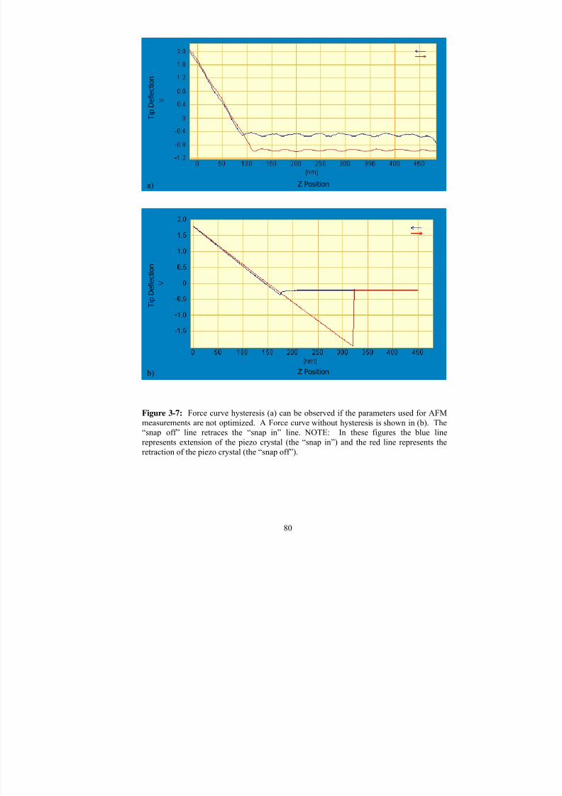
7/27/2019 Atomic Force Microscopy Method Development for Surface Energy Analysis
http://slidepdf.com/reader/full/atomic-force-microscopy-method-development-for-surface-energy-analysis 102/365
80
Figure 3-7: Force curve hysteresis (a) can be observed if the parameters used for AFMmeasurements are not optimized. A Force curve without hysteresis is shown in (b). The
“snap off” line retraces the “snap in” line. NOTE: In these figures the blue linerepresents extension of the piezo crystal (the “snap in”) and the red line represents theretraction of the piezo crystal (the “snap off”).
Z Position
T i p D
e f l e c t i o n
a)
b)
T i p D e f l e c t i o n
Z Position

7/27/2019 Atomic Force Microscopy Method Development for Surface Energy Analysis
http://slidepdf.com/reader/full/atomic-force-microscopy-method-development-for-surface-energy-analysis 103/365
81
3.4.2 Scan rate
The second parameter tested was scan rate. Scan rate and number of samples scanned per
area affect the speed at which the tip moves vertically and horizontally. When the scan
size is increased, the scan rate should be decreased to help prevent drift. However, when
scanning the same spot, scan rate did not have an effect on repeatability except in viscous
liquids, such as glycerol and ethylene glycol. Figure 3-7a shows hysteresis that occurs
when the scan rate is too fast in certain liquids. Figure 3-7 b shows what a force curve
looks like without hysteresis. It has been shown that hysteresis can affect the “true” force
between the tip and sample. A larger force is measured because the tip-sample distance
is greater than what it would be if the retracting curve was able to trace the advancing
line. Hysteresis can be minimized in most cases by slowing the scan rate. However, if a
liquid is too viscous, it can be difficult to execute AFM measurements and observe true
interactions between the sample and tip.
3.4.3 Force applied and contact area
Force applied and contact area, the next two parameters that were controlled, work
together. In order to maintain reproducible tip-sample interaction, the contact area must
be held constant throughout the experiments. Contact area impacts the depth the tip
penetrates into a sample. At different depths the tip can make contact with other chemical
moieties and this can cause variations in the forces. In Chapter 4, the elastic deformation
observed in the JKR model demonstrates this effect. The amount of force applied to the
tip will control the contact area. This relationship is seen in Table 4-1. The force
applied can vary depending on the softness of a sample. Since mica and graphite were
used in this study, a larger force could be applied. It is also important to be able to

7/27/2019 Atomic Force Microscopy Method Development for Surface Energy Analysis
http://slidepdf.com/reader/full/atomic-force-microscopy-method-development-for-surface-energy-analysis 104/365
82
maintain this constant force from initial measurement to the last measurement on a
sample surface. Within the force imaging controls, a trigger mode can be set, either
relative or absolute. Relative mode will maintain a constant force level defined by the
trigger threshold parameter, even if there are shifts from the defined setpoint (Figure
3-8). The absolute mode does not allow for applied force to be held constant. This mode
permits drift in the setpoint and the force applied (Figure 3-8). Relative mode was
chosen for better control over the contact area, as it is dependent upon applied force.
During setup, the force applied was kept constant between 10-12 nN. Section 3.6.3 will
discuss how to calculate force applied during measurements.

7/27/2019 Atomic Force Microscopy Method Development for Surface Energy Analysis
http://slidepdf.com/reader/full/atomic-force-microscopy-method-development-for-surface-energy-analysis 105/365
83
Figure 3-8: The two types of trigger mode used in AFM measurements are shown here.The plot shows the effect of drift on each of the trigger modes. Relative mode waschosen for the force measurements used in this study. This mode allows a constant force
to be sustained, which helps to maintain the contact area, a critical parameter in achievingconsistent AFM measurements.[49]

7/27/2019 Atomic Force Microscopy Method Development for Surface Energy Analysis
http://slidepdf.com/reader/full/atomic-force-microscopy-method-development-for-surface-energy-analysis 106/365
84
3.5 Statistical Analysis of AFM Measurements
The goal of this work is to measure the force of adhesion with the AFM and then
calculate surface energy. However, before surface energy can be determined, the force
data must be analyzed and understood. In all studies, multiple measurements on multiple
samples must be made to get a reliable result. Because of the substantial amount of data
generated, a statistical model was developed to help analyze the data and determine
which parameters caused the most error. The following steps were taken in order to
develop the statistical model:
1. Identify the variables that contribute to data collection. Determine a methodical
approach to measure forces with selected surfaces and tips that will allow for a
conclusion to be drawn.
2. Review data collection and decide on a statistical model that can incorporate the
variables.
3. Test the model.
The overall goal of a statistical model is to compare the averages of forces between
different samples and tips. In statistics, a way to look at this is with hypothesis testing.
The hypotheses being considered are typically formulated in terms of the null (H 0) and
alternative hypotheses (H1). For this study there are three hypotheses being tested. These
would be
Hypothesis 1:
H0: The variance (s2) between the locations, locations on each sample, locations
between each tip are similar.

7/27/2019 Atomic Force Microscopy Method Development for Surface Energy Analysis
http://slidepdf.com/reader/full/atomic-force-microscopy-method-development-for-surface-energy-analysis 107/365
85
H1: The variance (s2) between the locations, locations on each sample, locations
between each tip are not similar.
Hypothesis 2:
H0: The variance (s2) between each sample is similar.
H1: The variance (s2) between each sample is not similar.
Hypothesis 3:
H0: The variance (s2) between each tip is similar.
H1: The variance (s2) between each tip is not similar.
3.5.1 Identification of variables
The variables that may influence the force measurement are the samples (mica and
graphite), the tips, and the locations on the samples, as further explained below.
• Tips – The tips are necessary for any AFM measurement. This is an important
component for measuring forces, and therefore, can introduce large variability.
Tips will have variable radii which affect the contact areas. Also, if the tip radius
is not monitored, the user will not know when it becomes dull. A tip and
cantilever can also pick up small particulates in the air or liquids or on the sample
surface, which can change the tip characteristics and the resonance of the
cantilever. Therefore, to find the influence of the tip variation on force
measurements, it was thought that multiple tips should be tested. For statistical
power with the model three tips per condition were used.
7/27/2019 Atomic Force Microscopy Method Development for Surface Energy Analysis
http://slidepdf.com/reader/full/atomic-force-microscopy-method-development-for-surface-energy-analysis 108/365
86
• Samples (mica and graphite) – Mica and graphite were chosen as the samples
because they were inert to the solvents used in contact angle measurements, and
the surfaces are homogeneous and relatively smooth. It was also important to
evaluate the AFM’s ability to measure multiple samples to find the variability
among samples. For the statistical model to have power, two different sample
surfaces were used with each tip.
• Locations – On a sample surface, many spots can be tested. It was already shown
that the scan size should be 0 so that the data collected are meaningful. To have a
trusted value at one spot, multiple measurements (256 force curves) can be
obtained. Since these measurements are made in about a 5 to 15 nm2 area,
multiple areas on each sample should be measured to get an average surface
energy for each sample. Thus, one force value will be obtained from the average
of 256 force curves per spot. Sometimes these force curves will not have a
normal distribution, but because of the large data set, the central limit theorem
states that it can be assumed normal so that an average can be calculated.
Therefore, to extract enough data on one sample surface and evaluate the effect
location can have, ten locations were measured per sample.
The method for data collection described above is better illustrated in Figure 3-9. This
figure shows for each condition, two samples, three tips, and ten locations per sample
were measured. At the end of data collection, there should be 60 points of surface energy
data that can be evaluated over three tips and two samples. Table 3-1 helps to illustrate
the final results and how they can be split up for a statistical analysis. The headings for
each column are: sample (mica or graphite), tip, location, and SE (surface energy). In the

7/27/2019 Atomic Force Microscopy Method Development for Surface Energy Analysis
http://slidepdf.com/reader/full/atomic-force-microscopy-method-development-for-surface-energy-analysis 109/365
87
sample column there is either a 1 or 2, representing sample number 1 or sample number
2. In the tip column there is a 1, 2, or 3, representing tip 1, 2, or 3. In the location
column there are 10 numbers illustrating the ten locations data was collected. And
finally, in the last column, the average surface energy from 256 force curves at each of
the locations. (To illustrate this, the data from mica in diiodomethane was used. The
analysis of data will be discussed further in section 5.4.2.2. The presentation in this
chapter is to help demonstrate the statistical model.)
Once the method to collect data was chosen and the variables were defined, a statistical
model was selected. The repeated measures mixed model[50] was used because repeated
measures are made on a sample surface and the model has fixed (locations) and random
(sample, tip) variables. The model utilizes a repeated measures analysis of variance
(ANOVA) to calculate the F-value, which allows the user to accept or reject the null
hypothesis mentioned above that the variances between the tips, samples, and location is
similar.

7/27/2019 Atomic Force Microscopy Method Development for Surface Energy Analysis
http://slidepdf.com/reader/full/atomic-force-microscopy-method-development-for-surface-energy-analysis 110/365
88
Figure 3-9: Diagram of the number of mica or graphite samples, tips, and locationsevaluated using the AFM. This approach was used for all environmental conditions andsolvents.
Graphite/Mica 1 Graphite/Mica 2
Tip 1
Tip 2
Tip 3

7/27/2019 Atomic Force Microscopy Method Development for Surface Energy Analysis
http://slidepdf.com/reader/full/atomic-force-microscopy-method-development-for-surface-energy-analysis 111/365

7/27/2019 Atomic Force Microscopy Method Development for Surface Energy Analysis
http://slidepdf.com/reader/full/atomic-force-microscopy-method-development-for-surface-energy-analysis 112/365
90
For the statistical analysis, JMP (version 7, SAS Institute Inc., Cary, NC) and SAS
(version 6.11, SAS Institute Inc., Cary, NC) were used to calculate the F-value and
determine if there were differences among measurements. The output from SAS and
JMP are shown in Table 3-2a and b and Table 3-2c, respectively. The SAS output is a
typical ANOVA with the sum of squares, mean squared, F-values, and the corresponding
p values from the F distribution tables. From the SAS tables a decision can be made
whether to accept or reject the null hypothesis and if the surface energy data can be
combined. The p values are the probability of obtaining an experimental result as
different or more different than the expected result by chance alone. The p-value in
hypothesis testing is the α level, or significance level, at which one could accept or reject
the null hypothesis. The default α level is 0.05 and the null hypothesis is accepted when
p>0.05 and rejected when p<0.05. The data presented Table 3-2a and b shows the null
hypothesis could be accepted.
SAS Table 3-2a is the statistical analysis for within subjects, which is the variability of
the locations. If there is variability within the locations between tips or samples, then the
data set of one or all samples is statistically different. When the data is statistically
different, taking an average of the combined results will lead to an erroneous conclusion.
Instead, the experimental set up for measuring forces will have to be evaluated and
retested. An example of this will be discussed in Chapter 6.
SAS Table 3-2b is the statistical analysis between subject effects. The table shows the
comparison of all the samples and tips and evaluates the interaction between the samples
and tips. If there are statistical differences between mica or tips, combining the data and
calculating the average will result in an invalid conclusion. It would be better to present

7/27/2019 Atomic Force Microscopy Method Development for Surface Energy Analysis
http://slidepdf.com/reader/full/atomic-force-microscopy-method-development-for-surface-energy-analysis 113/365
91
the data separately. If the data is found to be statistically significant, then the repeated
measures mixed model would have found limitations in the AFM. These limitations
could be caused by the sample of interest or the conditions used to measure the forces.
If there are not statistical differences in location, mica, and tips, the JMP software is able
to evaluate which component contributes to the most variation, Table 3-2c. These tables
are used throughout Chapter 5 and 6 to show the AFM’s capability in making consistent
force of adhesion measurements and its challenges. The software is limited though
because it yields negative numbers when a variable or interaction being tested has no
contribution to the variability of the measurements. In these scenarios, the negative
numbers were made zero and the percent contributions of the others were recalculated.
For the example in Table 3-2, the null hypothesis was accepted, the data set was
combined and an average force, work, and surface energy value could be determined.
The JMP data shows that the largest variation comes from the residual error of the
measurements. Therefore, there are no apparent problems in evaluating mica-
diiodomethane with the AFM.

7/27/2019 Atomic Force Microscopy Method Development for Surface Energy Analysis
http://slidepdf.com/reader/full/atomic-force-microscopy-method-development-for-surface-energy-analysis 114/365
92
Table 3-2: Mixed model statistics for mica AFM measurements with diiodomethane. a)Repeated measures ANOVA for within subject effects, b) repeated measures ANOVA for between subjects, and c) the variable that demonstrates the largest percentage of variancefor mica – diiodomethane AFM measurements.
Degrees of
Freedom
Sum of
Square
Mean
Square F Value PLocation 9 16.1 1.8 1.48 0.23Location*Mica 9 12.7 1.4 1.17 0.37Location*Tip 18 34.7 1.9 1.60 0.16Error 18 21.7 1.2 - -
Degrees of Freedom
Sum of Square
MeanSquare
F Value P
Mica 1 12.3 12.3 3.27 0.21Tip 2 0.4 0.2 0.06 0.95Error 2 7.5 3.8 - -
Variable % of the Total % TruncatedMica 15.3 14.0Tip -9.5 0.0Mica*Tip 12.0 10.9Mica*Tip*Location (Error) 82.3 75.1
Total 15.3 14.0
a)
b)
c)

7/27/2019 Atomic Force Microscopy Method Development for Surface Energy Analysis
http://slidepdf.com/reader/full/atomic-force-microscopy-method-development-for-surface-energy-analysis 115/365
93
3.6 AFM Methodology
To use the AFM to investigate surface energy, force measurements were made in
ambient, controlled relative humidity (RH), and in the same liquids that were used in
contact angle measurements. Before discussing how the AFM can be used to evaluate
surface energy, this section will provide the details of the methods used to obtain forces.
3.6.1 Spring constant
Two methods were presented in Section 3.3. However, the goal was to have a
nondestructive method that could be used on each tip. Therefore, to employ the thermal
method as the main technique for measuring the spring constant of the AFM, studies
were done using the added mass method and then compared to results obtained from the
thermal method.
3.6.1.1 Added mass method
Resonance frequencies of ten silicon nitride cantilevers (Veeco, Camarillo, CA),
specifically 200μm narrow, were measured with a Nanoscope MultiMode AFM (Veeco,
Santa Barbara, CA) before and after a tungsten sphere was added, Figure 3-10.
The tungsten sphere was added using an Axiovert S100 (Zeiss, Thornwood, NY)
microscope. To get the tungsten sphere to adhere to the cantilever, epoxy was first
placed on the same side as the probe. Using a needle attached to a micromanipulator
(Eppendorf, Westbury, NY), a tungsten sphere was then added behind the probe,
Figure 3-11.
Scanning electron microscopy (SEM) images were taken of each sample using a Hitachi
S-4300 FE-SEM (Hitachi, Pleasanton, CA). The samples were coated with gold prior to

7/27/2019 Atomic Force Microscopy Method Development for Surface Energy Analysis
http://slidepdf.com/reader/full/atomic-force-microscopy-method-development-for-surface-energy-analysis 116/365

7/27/2019 Atomic Force Microscopy Method Development for Surface Energy Analysis
http://slidepdf.com/reader/full/atomic-force-microscopy-method-development-for-surface-energy-analysis 117/365
95
Figure 3-10: Resonance frequencies of silicon nitride cantilevers before (15.91 kHz) andafter (10.53 kHz) a tungsten sphere is added.

7/27/2019 Atomic Force Microscopy Method Development for Surface Energy Analysis
http://slidepdf.com/reader/full/atomic-force-microscopy-method-development-for-surface-energy-analysis 118/365
96
Figure 3-11: Addition of tungsten sphere. After the epoxy is added to the back of the
cantilever, a) the sphere is picked up by the needle, b) the needle is moved over the
cantilever, and c) then the tungsten sphere is placed on the cantilever and the needle is
retracted.
a) b)
c)

7/27/2019 Atomic Force Microscopy Method Development for Surface Energy Analysis
http://slidepdf.com/reader/full/atomic-force-microscopy-method-development-for-surface-energy-analysis 119/365
97
Table 3-3: Measured resonance frequencies, tungsten radii, and spring constant of tensilicon nitride cantilevers using the added mass method.
Sample Number Initial ResonanceFrequency (kHz)
ResonanceFrequency After
Added Sphere (kHz)
Radius
(μm)
k
(N/m)
1 15.88 9.95 10.5 0.06
2 17.54 11.20 8.8 0.05
3 15.91 11.25 8.9 0.06
4 17.44 8.91 12.0 0.06
5 15.88 11.09 10.2 0.08
6 15.96 9.60 10.6 0.05
7 16.05 10.70 9.70 0.06
8 15.97 8.68 12.2 0.06
9 15.91 9.33 11.3 0.06
10 15.91 10.53 9.20 0.06
Average 16.25 10.12 10.34 0.06
Standard Deviation 0.66 0.96 1.22 0.01

7/27/2019 Atomic Force Microscopy Method Development for Surface Energy Analysis
http://slidepdf.com/reader/full/atomic-force-microscopy-method-development-for-surface-energy-analysis 120/365
98
Figure 3-12: SEM image of a tungsten sphere added to an AFM cantilever.

7/27/2019 Atomic Force Microscopy Method Development for Surface Energy Analysis
http://slidepdf.com/reader/full/atomic-force-microscopy-method-development-for-surface-energy-analysis 121/365
99
3.6.1.2 Thermal Method
Before thermal vibration data could be collected, modifications had to be made to the
AFM MultiMode circuit board and controller. A cable was attached to pin 1 at U1 of the
analog to digital integrated circuit of the AFM, Figure 3-13. The other end of the cable
was attached to the controller analog channel 1. This connection allowed the signal to go
directly to the main controller and bypass electronic filters that manipulate the input
signal. The raw data from U1 is the vertical deflection (A-B), which outputs thermal
vertical vibrations. Once the set up was complete, instructions from Veeco were
followed to collect thermal vibrations. To determine the spring constant of a cantilever in
air or in a liquid:
1) Configure software for contact mode and engage microscope on a hard sample
surface. Mica (Ted Pella, Inc., Redding, CA) was used as the sample surface.
(NOTE: It is important that the laser position is not adjusted after this step.)
2) Once engaged, switch mode to Advanced Force Mode and set the following
parameters
a. Deflection setpoint – 0 Volts

7/27/2019 Atomic Force Microscopy Method Development for Surface Energy Analysis
http://slidepdf.com/reader/full/atomic-force-microscopy-method-development-for-surface-energy-analysis 122/365
100
Figure 3-13: Electronics board under the AFM stage that is manipulated to bypass filtersand measure raw thermal vibration to determine the cantilevers spring constant.

7/27/2019 Atomic Force Microscopy Method Development for Surface Energy Analysis
http://slidepdf.com/reader/full/atomic-force-microscopy-method-development-for-surface-energy-analysis 123/365
101
b. Ramp size – 500 nm
c. Trigger mode – Off
d. Input signal – Channel 1 (analog dial receiving raw data from U1)
e. Data scale – 20 Volts
f. Data center – 0 Volts
3) Adjust Z scan start until a force curve with 2-3 V of deflection relative to the
non-contact deflection value is obtained, Figure 3-14a.
4) Capture five forces and then switch back to image mode and disengage the
probe.
5) Go to the offline mode and view the force curves previously captured
individually to obtain the “Sensitivity”.
a. View → Graph → Sensitivity
b. Move the markers on the extend curve to the “contact region” of the force
curve, Figure 3-14b, so there is 1.5 – 2 V of deflection between them.
c. Record the average of the five force curves for Step 7a.
6) Go back to real time mode and set the following parameters:
a. Scan size = 0.01 nm
b. Scan rate = 61 Hz
c. Samples per line = 512
d. Lines = 512
7/27/2019 Atomic Force Microscopy Method Development for Surface Energy Analysis
http://slidepdf.com/reader/full/atomic-force-microscopy-method-development-for-surface-energy-analysis 124/365
102
e. Deflection setpoint = 0V
f. Channel 1 = input 1 (all other channels set to off)
g.
Real time planefit = none
h. Offline planefit = none
i. Deflection setpoint = 0 V
7) Go to Microscope → Calibrate → Detector
a. Input1 Sens – Average value from Step 5c (including units nm/V).
8) Ensure the tip is above the surface by withdrawing the tip 4 times. Force a false
engagement of the tip. The data will output quickly. Make sure the gains are set
to zero for I and P and that the Z center position is in the middle. Capture three
images and then withdraw the tip.
9) Switch to offline mode and double click on one of the files previously captured.
10) Go to Utility → ASCII Export and set:
a. Format = ASCII
b. Header = No
c. Image 1 units = nm
d. Number of columns = 1
e. Set filename and path desired to save
11) Each file was saved as a text file and imported into Matlab for further analysis.
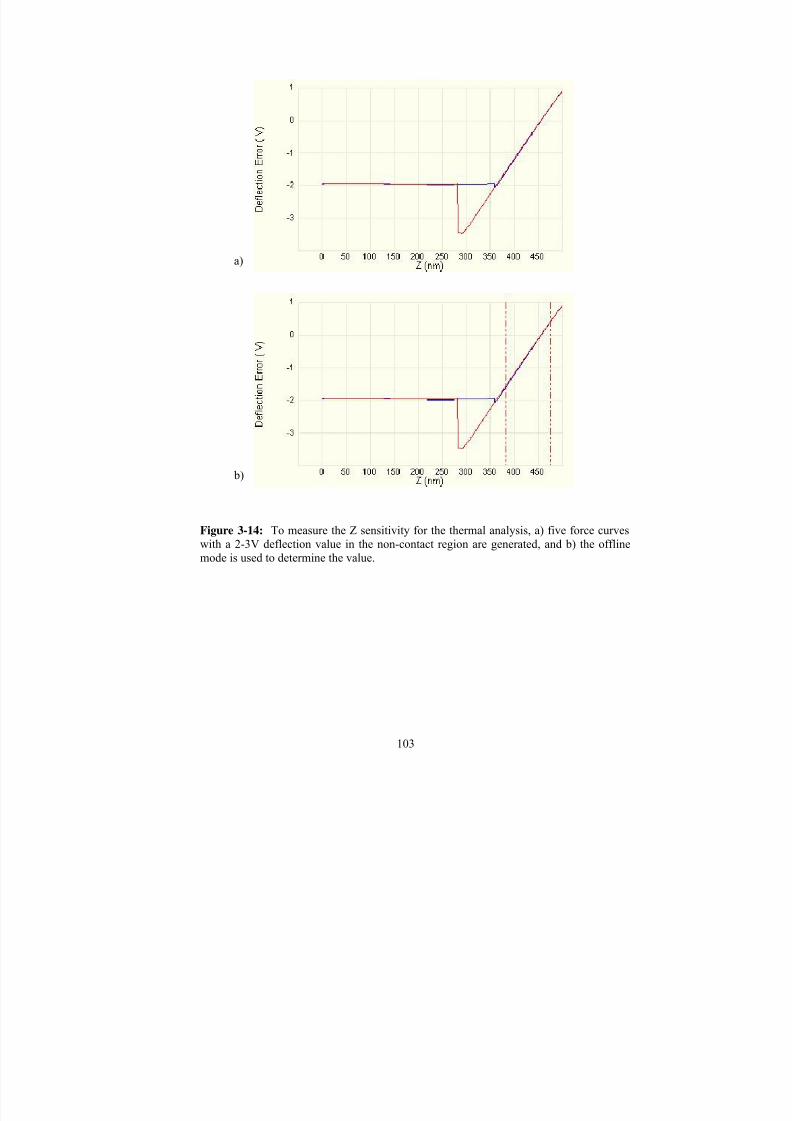
7/27/2019 Atomic Force Microscopy Method Development for Surface Energy Analysis
http://slidepdf.com/reader/full/atomic-force-microscopy-method-development-for-surface-energy-analysis 125/365
103
Figure 3-14: To measure the Z sensitivity for the thermal analysis, a) five force curveswith a 2-3V deflection value in the non-contact region are generated, and b) the offlinemode is used to determine the value.
a)
b)

7/27/2019 Atomic Force Microscopy Method Development for Surface Energy Analysis
http://slidepdf.com/reader/full/atomic-force-microscopy-method-development-for-surface-energy-analysis 126/365
104
The Matlab algorithm used to calculated the spring constant was designed to
automatically generate a report each time it was run. Please refer to Appendix 1 for an
example report and Appendix 2 for the code. The algorithm consisted of two main
functions, file input and spring constant calculation. It broke down into nine sub-
functions, which will each be addressed separately in the following discussion.
1) Import the tip file into a single vector (1 x 262144). The dimensions of this vector
come from the number of samples per line (512) and number of lines (512). Each AFM
measurement yields one thermal noise measurement.
2) To improve the precision of the Fourier Transform calculation, reshape the vector
into overlapping blocks of 4096.
3) Compute the Fourier Transform from each row of the reshaped matrix.
4) Compute the complex conjugate of the new matrix to keep real numbers and
eliminate imaginary numbers.
5) Compute the average of the rows to obtain a single vector (1 x 4096)
6) Smooth the output as necessary with either a moving boxcar, a cubic spline, or a 5-
point Savitzky-Golay smoothing filter. The cubic spline resulted in the most
appropriate and reproducible spring constant calculation.
7) Integrate the area under the smoothed resonant peak.
8) Calculate the spring constant k according to k = k b*T/A, where k b is the Boltzmann
constant, T is the temperature in degrees Kelvin, and A is the peak area.
9) Output the results of the spring constant calculation and plot the resonant peak to be
sure the correct area was selected.

7/27/2019 Atomic Force Microscopy Method Development for Surface Energy Analysis
http://slidepdf.com/reader/full/atomic-force-microscopy-method-development-for-surface-energy-analysis 127/365
105
Calibration of the spring constant was done on eight cantilevers from the same wafer as
the cantilevers used in the added mass study.
With the development of a method to continually monitor the spring constant of the
cantilever and the deflection acquired from the AFM measurements, the force of
adhesion can be calculated using Hooke’s Law. Since the primary focus of this study
was to determine surface energy using the AFM measurements, the next step was to
compute the work of adhesion. Surface energy was calculated after determining the force
and work of adhesion.
3.6.2 Tip radius
As with measuring the spring constant, the goal for determining tip radii was to have a
method for initial and repeated evaluation. Since the SEM images require a gold coating
and will destroy the tip, three tips were evaluated using the blind reconstruction method.
The sample used for the blind reconstruction was a tip tester (CSEM, Neuchâtel,
Switzerland). The scans were made in a 1000 X 1000 nm area at a rate of 1.97 Hz. The
relative trigger mode was employed, and the constant maximum loading force of 8-10 nN
was maintained. The scans were then analyzed in the SPIP software (Nanoscience
Instruments, Inc., Phoenix, AZ).
SEM images were taken of these tips and two unused tips with a Hitachi S-4300 FE-SEM
(Hitachi, Pleasanton, CA). Two unused tips were imaged under the SEM only to make
sure scanning did not affect the initial tip radius. Thus, these two tips were a baseline for
viewing and measuring the tip. The samples were coated with gold prior to imaging to
reduce charging and destruction of the sample. The electron beam was set to 3kV and the
current supplied was maintained at 10mA. The working distance was 15mm and the

7/27/2019 Atomic Force Microscopy Method Development for Surface Energy Analysis
http://slidepdf.com/reader/full/atomic-force-microscopy-method-development-for-surface-energy-analysis 128/365
106
condenser lens was set to 8. Since the SPIP software works based on a deconvolution of
the AFM images, comparison of the SPIP created image, Figure 3-15b, and the SEM
image, Figure 3-15a, became necessary to establish consistent parameters. Images from
SPIP were overlaid on the SEM images for each tip, Figure 3-15c, and a tip radius was
obtained, Table 3-4.

7/27/2019 Atomic Force Microscopy Method Development for Surface Energy Analysis
http://slidepdf.com/reader/full/atomic-force-microscopy-method-development-for-surface-energy-analysis 129/365
107
Figure 3-15: Determining tip radius with a) SEM image of a 200μm silicon nitride tip,b) SPIP image of the apex of the tip, and c) the image overlay, a combination of a and b.
a)
b)
c)

7/27/2019 Atomic Force Microscopy Method Development for Surface Energy Analysis
http://slidepdf.com/reader/full/atomic-force-microscopy-method-development-for-surface-energy-analysis 130/365
108
Table 3-4: AFM tip radii measured from blind reconstruction and compared with SEMimages. The first two tips were only imaged using the SEM as a baseline.
Tip
SEM
Tip Radius
(nm)
BlindReconstruction
Tip Radius(nm)
1 48 N/A
2 52 N/A
3 47 42
4 46 38
5 48 40

7/27/2019 Atomic Force Microscopy Method Development for Surface Energy Analysis
http://slidepdf.com/reader/full/atomic-force-microscopy-method-development-for-surface-energy-analysis 131/365
109
The manufacturer of the silicon nitride tip reports a maximum tip radius of 40 nm. The
results from the SEM images illustrate the method does overestimate the tip radius. The
results from the blind reconstruction varied depending on the settings input for the blind
reconstruction in the SPIP. If there were not enough iterations, the reconstruction would
be smaller than the SEM image, and with too many iterations, the reconstructed tip is
larger than the SEM image. Therefore, creating the overlaid image helped provide
guidance for the required input. Although it was not possible to image each tip used over
all the AFM experiments, the SEM image in Figure 3-15a was consistently used as a
reference for overlaying all blind reconstruction images produced by SPIP. The tip
radius was checked after a standard set of measurements. Once the tip radius was 10 nm
larger than the initial measurement, the tip was discarded and a new tip was
characterized.
3.6.3 AFM scanning parameters
There were four parameters identified as critical to control during force measurements.
The following was done to control scan size, scan rate, force applied, and contact area.
The scan size of each point was 0 nm. At each point 256 force curves were collected and
then the tip was moved to a different spot on the sample, as described in Section 3.5. The
scan rate can be set at 5 to 8 Hz when measuring forces in vapor and non-viscous liquids.
In viscous liquids, like ethylene glycol, the scan rate must be reduced to 3 Hz or smaller.
The applied force can be calculated from the graph shown in Figure 5.4 The spring
constant and Δz (from contact with the surface to the piezo crystal beginning retraction)
shown in Figure 3-16 need to be found. These values are used by the on-line control
program to calculate the force.

7/27/2019 Atomic Force Microscopy Method Development for Surface Energy Analysis
http://slidepdf.com/reader/full/atomic-force-microscopy-method-development-for-surface-energy-analysis 132/365
110
F = k * Δz
Δz = number of divisions horizontally * x scale * Z piezo sensitivity.
The value can be determined more precisely with the SPIP software, but a wide range of
10-12nN allowed for flexibility in estimating the applied force in-line following these
guidelines.
1. Determine the Z piezo sensitivity. The instructions to do so were covered in
Section 3.3, under the methodology for determining spring constant with the
thermal method.
2. The x scale is the Z Position and has (V/div) as the units of measure.
3. The number of divisions is counted by starting at the very left edge of the graph
and counting over to the start of the triangle.
Once these parameters are determined, the force applied can be calculated. If the force
calculated was not between 10 – 12 nN, then the trigger threshold in the Z scan controls
box will have to be changed until it is. The trigger threshold allows for increase and
decrease in force applied by shifting the force curve right and left.

7/27/2019 Atomic Force Microscopy Method Development for Surface Energy Analysis
http://slidepdf.com/reader/full/atomic-force-microscopy-method-development-for-surface-energy-analysis 133/365
111
Figure 3-16: The force curve and parameters used to determine the force applied.[49]The horizontal divisions are counted until the first marked (+). It is important to estimatethe number of divisions as close as possible noting the best calculation will be obtained
from the SPIP software.

7/27/2019 Atomic Force Microscopy Method Development for Surface Energy Analysis
http://slidepdf.com/reader/full/atomic-force-microscopy-method-development-for-surface-energy-analysis 134/365
112
3.6.4 AFM measurements
In order to evaluate the AFM’s potential use for studying surface energetics, the same
samples used in the contact angle studies, Section 2.3, were used for the AFM studies.
The conditions initially tested were in ambient environment without any control of
moisture content to determine solid-vapor surface energy. Next, the vapor measurements
were repeated, but in a controlled humidity environment. A near zero percent humidity
was achieved by purging and environmental chamber with nitrogen gas. Last, the solid-
liquid surface energy was determined using the same liquids that were used in the contact
angle measurements (water, diiodomethane, ethylene glycol, and formamide). Since
there were variations in the contact angles using hydrated liquids, the hygroscopic liquids
were dried before measuring forces. All force curves are then analyzed using SPIP
software (Nanoscience Instruments, Inc., Phoenix, AZ).
3.6.4.1 Ambient humidity measurements
The effects of humidity on the pull-off force has been previously studied.[51-53] It has
been shown that stiff cantilevers can lessen the impact humidity has on the force
measurements. However, if a flexible cantilever is used, which is best for sensitivity,
then humidity has a major impact on the force measurements. The more humidity
present the larger the spread or range in the force of adhesion. Therefore, if a flexible
cantilever is used, the environmental conditions have to be controlled. In this study, it
was important to compare the difference between ambient and controlled conditions.
Also the contact angle measurements were made in ambient conditions, and therefore
could be more comparable to AFM results in ambient environment. The ambient

7/27/2019 Atomic Force Microscopy Method Development for Surface Energy Analysis
http://slidepdf.com/reader/full/atomic-force-microscopy-method-development-for-surface-energy-analysis 135/365
113
environmental conditions for the three tips and two samples of mica and graphite were
measured at 23-26ºC and 59-62% relative humidity (RH) measured with a hand held
hygrometer. The tip holder for measurements in vapor is shown in Figure 3-17.
3.6.4.2 Controlled relative humidity measurements
After the forces were measured in ambient conditions, three new AFM tips and the two
mica samples were then placed in a desiccator. Air was pulled out of the desiccator with
a vacuum pump. The samples were held in the desiccator for 24 hours. The samples
were then transferred individually to the AFM and the measurements were made in an
environmental chamber with less than 10% relative humidity. To create low humidity in
the environmental chamber, nitrogen gas was purged for two hours, while monitoring the
relative humidity with a hygrometer. The AFM set up with the environmental chamber is
shown in Figure 3-18.

7/27/2019 Atomic Force Microscopy Method Development for Surface Energy Analysis
http://slidepdf.com/reader/full/atomic-force-microscopy-method-development-for-surface-energy-analysis 136/365
114
Figure 3-17: Bottom side of a tip holder for vapor measurements. The gold piece holdsthe cantilever.
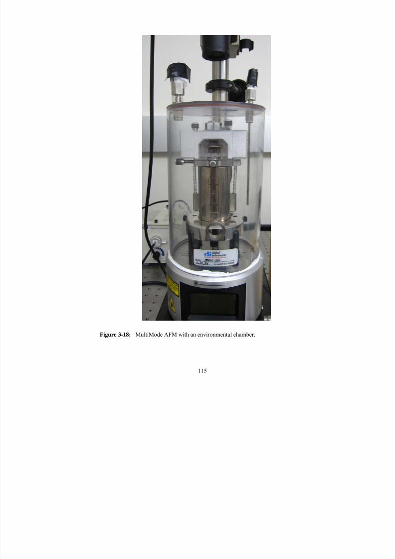
7/27/2019 Atomic Force Microscopy Method Development for Surface Energy Analysis
http://slidepdf.com/reader/full/atomic-force-microscopy-method-development-for-surface-energy-analysis 137/365
115
Figure 3-18: MultiMode AFM with an environmental chamber.

7/27/2019 Atomic Force Microscopy Method Development for Surface Energy Analysis
http://slidepdf.com/reader/full/atomic-force-microscopy-method-development-for-surface-energy-analysis 138/365
116
3.6.4.2 Liquid measurements
Force measurements with mica and graphite samples were made in water, diiodomethane,
ethylene glycol, and formamide using a fluid cell, Figure 3-19. The fluid is injected
through a syringe and contained in an o-ring, Figure 3-20. The fluid was injected, but
because of interactions that can happen between the liquid and the surface, ten minutes
was given to allow for a so-called "equilibrium". It was observed that measurements
were less repeatable right after the liquid was injected. Thus, 10 minutes was allowed so
that the "equilibrium" between the liquid and the sample surface could be attained. The
measurements from formamide and ethylene glycol were made after the solvents had
been dried and with the rehydrated solvents, as with contact angle measurements in
Chapter 2.
In Chapter 6, additive solutions will be needed to measure forces on crystalline surfaces.
The methodology will be discussed further in that chapter, but it needs to be highlighted
that these types of solutions can be used with the AFM but could not be used with contact
angle measurements. The set up for the additive solutions is the same. The fluid cell and
syringe are used to introduce the liquid to the system. It is important to ensure the
additive has completely dissolved in the solvent before use. Thus, when an aliquot is
taken for injection, the concentration of the solution will be known.

7/27/2019 Atomic Force Microscopy Method Development for Surface Energy Analysis
http://slidepdf.com/reader/full/atomic-force-microscopy-method-development-for-surface-energy-analysis 139/365
117
Figure 3-19: Fluid cell used to measure forces with solvents and solutions.

7/27/2019 Atomic Force Microscopy Method Development for Surface Energy Analysis
http://slidepdf.com/reader/full/atomic-force-microscopy-method-development-for-surface-energy-analysis 140/365

7/27/2019 Atomic Force Microscopy Method Development for Surface Energy Analysis
http://slidepdf.com/reader/full/atomic-force-microscopy-method-development-for-surface-energy-analysis 141/365
119
3.7 Summary
The goal of this work is to use the AFM to investigate surface energy. This chapter
presented the components and functions of the AFM and the methodology developed for
force measurements with the AFM. The most important development in this chapter was
establishing methods for measuring the cantilever spring constant and the tip radius. A
scanning methodology was developed and a statistical model was chosen that will allow
for comparison and error analysis.
Tip characterization is an important step for measuring forces and calculating surface
energy. To calculate the force of adhesion from Hooke’s Law, deflection and the spring
constant are needed. The deflection is obtained from AFM data and then the forces can
be determined in SPIP. To obtain an accurate force, a spring constant needs to be entered
into the software. The spring constant has been determined using several methods;
however, the goal was to be able to measure the spring constant of each cantilever. The
value provided from the manufacturer and the destructive method was determined to be
unsuitable. The literature for the thermal method was reviewed and modifications were
made on the microscope to collect the data. A Matlab code was developed to analyze the
AFM data. The calculated spring constant from the thermal method was successfully
compared to the “gold standard” added mass method, allowing continued use of the
thermal method for determining the spring constant of every tip.
Tip radius will be a required parameter in Chapter 4 to finally calculate surface energy,
and therefore, a nondestructive method was needed to evaluate the radius of each tip.
The blind reconstruction literature was reviewed and then successfully implemented as
7/27/2019 Atomic Force Microscopy Method Development for Surface Energy Analysis
http://slidepdf.com/reader/full/atomic-force-microscopy-method-development-for-surface-energy-analysis 142/365
120
compared to the manufacturer’s value and SEM images. Thus, a method was developed
to continually monitor the tip radius.
The scanning methodology for force measurements in vapor and in liquids was discussed
and will be expanded upon in Chapters 5 and 6 to collect AFM data. The scan size, scan
rate, and applied force parameters were determined for AFM measurements in vapor and
in liquid. Finally, a repeated measures mixed model was implemented for statistical
analysis of the AFM data. The statistical model will allow for comparison between
samples and tips and show what contributions cause significant error.
The successful completion of the literature review and the AFM methodology of this
chapter set the stage for taking force measurements from the AFM and calculating
surface energy. To do this the next chapter will investigate various models with the goal
of determining surface energy.
Copyright © Clare Aubrey Medendorp 2011

7/27/2019 Atomic Force Microscopy Method Development for Surface Energy Analysis
http://slidepdf.com/reader/full/atomic-force-microscopy-method-development-for-surface-energy-analysis 143/365
121
Chapter 4 – AFM Math Models
The previous chapter evaluated the methodology of the AFM to measure forces.
However, the overall goal is to evaluate the AFM’s capability to investigate surface
energy. Therefore, models had to be developed to transform the force data into surface
energy. Currently, there is not an experimental method to measure surface energy
directly; as a result, all techniques require models. The model development for the AFM
force data is presented in this chapter
4.1 Contact Mechanics
In contact angle measurements, the spreading of a liquid over a surface to reach
equilibrium is dominated by the minimization of surface free energy. When two solids
are in contact, reaching the equilibrium state depends on the distribution of elastic forces.
Mechanical work must be expended to overcome the adhesive forces keeping two
separate bodies in contact. This work is involved in the creation of a new surface. Hertz
was the first to observe the contact between two smooth elastic bodies. When no surface
forces act, the contact area for two spheres with radius R 1 and R 2 pressed together under
load P is given by[54]
PR R
R R )k k (
4
3a
21
2121
30 +
+= π 4.1
where k 1 and k 2 are the elastic constants of the material of the spheres and k 1 and k 2 are
defined by

7/27/2019 Atomic Force Microscopy Method Development for Surface Energy Analysis
http://slidepdf.com/reader/full/atomic-force-microscopy-method-development-for-surface-energy-analysis 144/365
122
1
21
1E
1k
π
v−= and
2
22
2E
1k
π
v−= 4.2
where v is the Poisson ratio and E is the Young’s modulus of each material. Typically,Equation 3.7 is written in a simplified form
K
RPa =3
0 4.3
where R=R 1R 2/(R 1+R 2) and K=4/3π(k 1+k 2). To verify this theory, Hertz used an optical
microscope to measure the contact between two glass spheres. Hertz showed that both
the size and shape of the zone of contact followed from the elastic deformation of the two
glass spheres. Later, however, there were experimental contradictions observed to the
Hertzian theory. At low loads, the contact area was considerably larger than what Hertz
had predicted. Strong adhesion was observed and as the load was reduced toward zero, a
constant finite value of contact area was observed. This suggested that attractive surface
forces became important as the load was reduced towards zero, but at high loads Hertz
theory still held.[54]
Two contact mechanics models, Johnson-Kendall-Roberts (JKR)[54] and Deryaguin-
Muller-Toporov (DMT),[55] were developed to evaluate this relationship. The major
difference between the two models is the area each takes into account the energy of
molecular attraction. The JKR model takes into account what happens inside the area of
contact and DMT considers outside of the contact area. Therefore, the differences
observed in the applied force, contact radius, and deformation are due to the role
adhesion plays in the system. Table 4-1 summarizes the relationships for each model

7/27/2019 Atomic Force Microscopy Method Development for Surface Energy Analysis
http://slidepdf.com/reader/full/atomic-force-microscopy-method-development-for-surface-energy-analysis 145/365
123
of the contact radius, deformation of the sample, and force of adhesion. Using the tip
radius, R, (determined by blind reconstruction in Section 3.6.2) the work can be
calculated with the adhesion forces determined from AFM measurements.[32, 54, 55]
Then, contact radius can be calculated as a function of the reduced Young’s modulus, K,
which is
⎟⎟ ⎠
⎞⎜⎜⎝
⎛ −+
−=
t
t
s
s
E
v
E
v
K
22 11
4
31 4.4
where vt, Et, vs, and Es are the Poisson’s ratio and Young’s modulus of the tip and the
sample respectively. Lastly the deformation of the sample can be determined.
Figure 4-1a, shows the interaction between completely rigid particles and Figure 4-1b,
shows particles that deform when they come into contact. JKR showed that the attractive
surface forces pull the two surfaces together giving rise to a finite contact area, even
under zero external load. When surface forces are not observed (W=0), the JKR and
DMT contact area equations revert back to the simple Hertz equation (4.3). For the JKR
model when the applied load is made negative, the contact radius decreases. Thus, for a
solution to be obtained
( )236 RW RPW π π ≤ ,
RW P π 2
3
−≥
4.5
and separation of the sphere will occur when

7/27/2019 Atomic Force Microscopy Method Development for Surface Energy Analysis
http://slidepdf.com/reader/full/atomic-force-microscopy-method-development-for-surface-energy-analysis 146/365
124
RW P π 2
3−= 4.6
Thus, equation 4.6 illustrates that the applied force does not affect force of adhesion. It
only affects the contact area that the AFM tip will observe, as discussed in Chapter 3.
However, because of the sensitivity of the AFM and its capability to resolve sub-
angstrom, force applied should be monitored. This will help control contact area so the
load does not push the tip into several different chemical moieties.
Similarly for the DMT model, a solution can be obtained as long as
RW P π 2−≥ 4.7

7/27/2019 Atomic Force Microscopy Method Development for Surface Energy Analysis
http://slidepdf.com/reader/full/atomic-force-microscopy-method-development-for-surface-energy-analysis 147/365

7/27/2019 Atomic Force Microscopy Method Development for Surface Energy Analysis
http://slidepdf.com/reader/full/atomic-force-microscopy-method-development-for-surface-energy-analysis 148/365
Figure 4-1: a) An illustration of a rigid sphere on a rigid surface. b) On the left is an illustration of asurface in the absence of adhesion (Hertz) and in the presence of adhesion (JKR). On the right is an elseparate from adhesive contact. [56]
R R
δ
a
a
r
F
Configuration at
equilibrium and pull-off
Equilibrium Pul
a) Rigid sphere b) Deformable (elastic) sphere
KR
Hertz
1 2 6

7/27/2019 Atomic Force Microscopy Method Development for Surface Energy Analysis
http://slidepdf.com/reader/full/atomic-force-microscopy-method-development-for-surface-energy-analysis 149/365
127
Since two models were developed that established the relationship between force and
work, Tabor developed a parameter to aid in the decision of which model should be used
based on AFM tip properties and the sample’s surface properties:[57]
( )( )3
02
3/12
zK
Rγ φ = 4.8
where R is the radius of the sphere (or AFM tip radius), γ is determined from contact
angle measurements, K is the reduced Young’s modulus that occurs at contact, and z0 is
the equilibrium size of atoms at contact. The value the average atomic diameter of
carbon (0.154 nm) was used for z0, by assuming the tip and the surface were in atomic
contact. When φ is greater than 0.3 the JKR model is used, when it is less than 0.3 the
DMT theory is used. This equation requires prior knowledge of the sample's surface
energy. In this study, the surface energy will come from contact angle, but other studies
have used surface energy information from inverse gas chromatography.[52] To obtain
tip radius, blind reconstruction (Section 3.6.3) is used.
Now that the methodology for measuring forces has been defined and the adhesion
models have been identified to take force and calculate work, the next step will be to take
the work of adhesion and determine surface energy. The illustration below is the
overarching goal to take AFM forces and determine surface energy
γ →→ W F 4.9

7/27/2019 Atomic Force Microscopy Method Development for Surface Energy Analysis
http://slidepdf.com/reader/full/atomic-force-microscopy-method-development-for-surface-energy-analysis 150/365
128
4.2 Surface Energy Models
In Section 2.2, the concepts and equations for the free energy of cohesion and adhesion
were introduced. These same principles are still applicable with the AFM, and just like
with contact angle measurements, mathematical models must be developed to interpret
the AFM data. There are no experimental methods that can be used to determine surface
energy directly and stopping at work of adhesion is not the goal. The work of adhesion
results makes it difficult to compare to contact angle and literature surface energy.
Continuing to surface energy will give more information about the individual surfaces
and it can be applied to understanding interactions with other solids and liquids.
Therefore, to determine the surface energy of a material in vapor or in a liquid using the
AFM:
• First, forces are measured,
• Second, the work of adhesion is calculated, and
• Finally, the surface energy is calculated through development of a robust model.
The next few sections will present possible models to use when investigating surface
energy with the AFM.
4.2.1 Surface energy model 1
In Section 2.2 and Figure 2-2, the change in surface free energy to separate two different
media, 1 and 2, in a third medium is given by:[56]
122313123 γ γ γ ++=W 4.10
7/27/2019 Atomic Force Microscopy Method Development for Surface Energy Analysis
http://slidepdf.com/reader/full/atomic-force-microscopy-method-development-for-surface-energy-analysis 151/365
129
where in air γ13, γ23, and γ12 represent the tip-vapor, sample-vapor, and tip-sample
respectively, and in a liquid represent tip-liquid, sample-liquid, and tip-sample,
respectively. Therefore, by measuring the adhesion force with the AFM it is possible to
determine the surface energy of sample-vapor or sample-liquid. However there are three
unknowns in Equation 4.10,
1. γ13 – tip-vapor or tip-liquid
2. γ23 – sample-vapor or sample-liquid
3. γ12 – sample-tip
In order to determine γ23 (γsv
or γsl) in Equation 4.10, the surface energy of the γ12 and γ13
must first be calculated. Therefore, more experiments were set up in order to achieve this
goal.
The tip-vapor and tip-liquid (γ13) surface energies will be obtained by measuring the
adhesion force between a pair of identical tips in air or in liquid (Figure 4-2). An AFM
tip scans the surface of the cantilever behind the AFM probe and the pull off force is
measured and work is calculated. It is worthwhile to point out that it is not necessary to
measure the force curve at the apex of the scanned tip because the entire cantilever and
tip are composed of the same silicon nitride. Thus, when similar materials are brought
together, the work of cohesion to pull them apart is equal to[56]
tvW γ ⋅=2 ; tlW γ ⋅=2 4.11
where γtv and γtl are tip-vapor and tip-liquid surface energies respectively.

7/27/2019 Atomic Force Microscopy Method Development for Surface Energy Analysis
http://slidepdf.com/reader/full/atomic-force-microscopy-method-development-for-surface-energy-analysis 152/365
130
Figure 4-2: Tip-tip AFM scans are performed in both vapor and liquid environments todetermine the tip-vapor and tip-liquid surface energies.

7/27/2019 Atomic Force Microscopy Method Development for Surface Energy Analysis
http://slidepdf.com/reader/full/atomic-force-microscopy-method-development-for-surface-energy-analysis 153/365
131
The third term, sample-tip (γ12), could not be determined from separate AFM
experiments. Therefore, going back to Equation 4.10, there are still two unknowns;
1. γ12 – sample-tip
2. γ23 – sample-vapor or sample-liquid
Consequently, this model could not be used to determine either γsv and γsl without
knowing γst first. To circumvent the limitation, the following is implemented:
1. Using contact angle measurements as described in Chapter 2, γsv can be
determined,
2. Then tip-tip measurements provide the surface energy of the tip in air, and
3. The work is calculated from force of adhesion measurements of the sample in air.
These steps lead to determining the γst based on Equation 4.10 when the medium is vapor.
The γst will then be used in:
st tlslstlW γ γ γ ++= 4.12
For γsl (solid-liquid surface energy) to be calculated the following
measurements/parameters must be defined:
1. AFM force of adhesion measurements on the sample surface in a solvent,
2. Calculation of work of adhesion from the forces obtained in the first item, and
3. Tip-tip AFM measurements in the same liquid to determine γtl, Equation 4.11.

7/27/2019 Atomic Force Microscopy Method Development for Surface Energy Analysis
http://slidepdf.com/reader/full/atomic-force-microscopy-method-development-for-surface-energy-analysis 154/365
132
Since there are several experiments and equations that are necessary to achieve the final
goal, a flow chart in Figure 4-3 has been developed.
In order to use this model for determining solid-liquid surface energy, a few assumptions
were made. First, since contact angle measurements were used it was assumed that the
liquids used for contact angle measurements did not influence the determination of solid-
vapor surface energy, and it would be constant over any combination of liquids. This
assumption is difficult to make because most of the indirect models used to determine
solid-vapor surface energy warn against this.[2, 9] All of these models rely on fitting
results from various liquids. If a different combination of liquids is chosen, the
calculated solid-vapor surface energy could be different. Thus, it is difficult to use
unreliable data from a second method. Also, the goal is to investigate the performance of
just the AFM for determining surface energy. The use of the AFM would be extremely
limited if the mathematical model needed to rely on another experimental method to
obtain the parameter of interest.
The second assumption is that the sample surface from the contact angle measurements is
comparable to the surface used for AFM measurements and remains unchanged in liquid
environments. Hence, the surface-tip surface energy will be the same in vapor as it is in
liquids. This assumption is difficult to make unless the material is inert in the liquid
being used. If the liquid interacts with the sample, possibly rearranging the surface
molecules, the sample-tip surface energy will vary. This was also a problem with contact
angle measurements. If the liquid deforms the surface, the measured contact angle is not
as accurate as an angle measured on a non-deformable surface.

7/27/2019 Atomic Force Microscopy Method Development for Surface Energy Analysis
http://slidepdf.com/reader/full/atomic-force-microscopy-method-development-for-surface-energy-analysis 155/365
133
Further investigation presented in Chapter 5 will also show the differences in solid-vapor
surface energy when measured in ambient and controlled relative humidity. These data
are more evidence that 1) using contact angle data for an AFM model is inadequate, and
2) the surface forces are different when water vapor is not present. However, since the
sample-tip surface energy is currently not measurable, the assumption that it is constant
must be made to use this model. The limitations discussed for this model are what led to
the development of another model.

7/27/2019 Atomic Force Microscopy Method Development for Surface Energy Analysis
http://slidepdf.com/reader/full/atomic-force-microscopy-method-development-for-surface-energy-analysis 156/365
134
Figure 4-3: Experimental flow chart in order to study solid-liquid surface energy usingthe AFM and mathematical model 1.
xk F Δ⋅−=
R
F W
π 3
2=
st tvsvW γ γ γ −+=
tvW γ 2=
xk F Δ⋅−=
R
F W
π 3
2=
tlW γ 2=
st tlslW γ γ γ −+=

7/27/2019 Atomic Force Microscopy Method Development for Surface Energy Analysis
http://slidepdf.com/reader/full/atomic-force-microscopy-method-development-for-surface-energy-analysis 157/365
135
4.2.2 Surface energy model 2
The second model eliminates relying on contact angle for determining the solid-vapor
surface energy. This model, the geometric mean, is based on an existing theory
continually used in the literature.[58]
tvsvW γ γ 2= 4.13
In section 2.2, the geometric mean and the mathematical assumptions that are made to
evaluate the free energy of two dissimilar surfaces were reviewed. The geometric mean
makes it possible to predict properties of the 12 interface from the separate properties of
the 1 and 2 phases. Hence, the surface-tip-vapor interactions are based on the solid-vapor
and tip-vapor phases. The elimination of γst from the equation leaves only one unknown,
γsv. Therefore to calculate solid-vapor surface energy (γsv) the following studies are done
1. Measure the forces of adhesion on the sample surface in vapor,
2. Calculate the work of adhesion from the forces obtained in the first item, and
3. Make tip-tip AFM measurements in vapor to determine γtv, Equation 4.11
These same steps can be followed to obtain solid-liquid surface energy, and Equation
4.13 becomes
tlslW γ γ 2= 4.14
The only difference is the force measurements for the sample and tip are done in a liquid
environment. The work flow to use this model and obtain solid-vapor and solid-liquid
surface energies is illustrated in

7/27/2019 Atomic Force Microscopy Method Development for Surface Energy Analysis
http://slidepdf.com/reader/full/atomic-force-microscopy-method-development-for-surface-energy-analysis 158/365
136
Figure 4-4. Compared to the first model, fewer experiments are required for the second
model, no assumptions have to be carried from the solid-vapor experiments to the solid-
liquid experiments, and contact angle data is not required to eliminate an unknown value.
This allows each set of measurements to be independent of the other, which the first
model could not do.
The assumption for this model is that the geometric mean can 1) be used with the AFM
and 2) the surface energy of the two separate phases (solid-vapor, tip-vapor) can be used
to represent the interaction of the sample-tip (the dissimilar phases). The geometric
mean, as mention in Section 2.2, only takes into consideration the van der Waals
interactions and does not include polar/hydrogen bonding forces. However, it has been
pointed out that the AFM measures the sum of all the forces occurring between the tip
and the sample. These forces can consist of capillary, electrostatic, and Liftshitz-van der
Waals forces.[58] The assumption that has to be made is the biggest limitation of this
model. It was shown that using the geometric mean model overestimates the surface
energy for contact angle measurements.[2, 9, 26, 59] Since the geometric mean model
was developed based on van der Waals interactions, it might be difficult to employ this
model with polar surfaces (mica). The best use of this model would be with surfaces that
mainly consist of London dispersion forces (graphite).
Because of the limitations with the geometric mean, Neumann’s lab added a modification
to correct for the overestimation of the geometric mean.[19, 20] It was thought this same
modification could be applied to the AFM, and therefore, another model should be tested.

7/27/2019 Atomic Force Microscopy Method Development for Surface Energy Analysis
http://slidepdf.com/reader/full/atomic-force-microscopy-method-development-for-surface-energy-analysis 159/365
137
Figure 4-4: Experimental flow chart in order to study solid-liquid surface energy usingthe AFM and mathematical model 2.
(Note: Model 3 follows the same flow diagram; the only difference is the solid-liquidsurface energy.)
xk F Δ⋅−=
R
F W
π 3
2=
tvsvW γ γ 2=
tvW γ 2=
xk F Δ⋅−=
R
F W
π 3
2=
tlsvW γ γ 2=
tlW γ 2=

7/27/2019 Atomic Force Microscopy Method Development for Surface Energy Analysis
http://slidepdf.com/reader/full/atomic-force-microscopy-method-development-for-surface-energy-analysis 160/365
138
4.2.3 Surface energy model 3
The third surface energy applies the modified geometric mean equation from contact
angle measurements to the AFM measurements.[59]
( )2
2 tvsveW tvsv
γ γ β γ γ
−−= 4.15
and in liquid environments the solid-liquid surface energy can be determined by:
( )2
2 tlsleW tlsl
γ γ β γ γ
−−= 4.16
The experimental flow of this model is similar to the one shown in
Figure 4-4. The only difference is the corresponding equations that will be used. One
difficulty with using this model is that the unknown variable which is being solved for,
solid-vapor or solid-liquid surface energy, is in both the exponential and under the square
root of the equations. For this reason, solving for these unknowns requires software that
can run iterations until the surface energy is solved.
Another limitation of this model is the assumption that β, a universal constant from
Neumann’s lab, can be translated to use with the AFM. In order to consider deviations
from the geometric mean, researchers have tried to introduce an empirical parameter that
is used as a correction factor.[25] The proposed correction factor by Neumann included
the universal constant β where β = 0.0001247 m
4
mJ
-2
. This value was obtained by
fitting large sets of experimental contact angle data. The data encompassed apolar, polar,
aprotic, and protic liquids on low energy polymeric surfaces. The scope of this
development was not to repeat such experiments to see if a universal parameter could be

7/27/2019 Atomic Force Microscopy Method Development for Surface Energy Analysis
http://slidepdf.com/reader/full/atomic-force-microscopy-method-development-for-surface-energy-analysis 161/365
139
established with the AFM. Thus, the assumption was made that this constant could be
applied the AFM studies. However, in Chapter 5 when the models are tested, the
influence of β will be explored to determine its effect on the fitting and iterations. The
values between models 2 and 3 will also be compared to determine if the addition of a
correction factor has any implications in calculating surface energy.
4.2.4 Surface energy model 4
In models 2 and 3 both solid-vapor and solid-liquid surface energies could be measured
using the AFM. Model 1 was not able to evaluate both. Since there were no direct ways
to measure γst, contact angle solid-vapor data had to be used. More evaluation was given
to model 1, and it was thought that if model 2 or 3 could be used to determine solid-vapor
surface energy, a mixed model could be developed (Figure 4-5). Then, γst would be
determined by
1. Measuring the forces of adhesion on the sample surface in vapor,
2. Calculating the work of adhesion from the forces obtained in the first item,
3. Making tip-tip AFM measurements in vapor to determine γtl, Equation 4.11, and
4. Using model 2 or 3 to calculate γsv.
Once these experiments were completed, the value for γst could be obtained. The surface-
tip surface energy can then be used in Equation 4.12 to investigate the solid-liquid
surface energy.
The mixed model would eliminate the need to use another technique for solid-vapor
surface. Thus negating the assumption that the surface measured in contact angle
7/27/2019 Atomic Force Microscopy Method Development for Surface Energy Analysis
http://slidepdf.com/reader/full/atomic-force-microscopy-method-development-for-surface-energy-analysis 162/365
140
measurements was the same as the surface used for AFM measurements. However, the
mixed model still requires that γst be evaluated. If any changes happen at the molecular
level on the surface in a liquid environment, the sample-tip surface energy will be
affected. Any changes to this surface energy cannot be captured until there is a direct
way to measure the sample-tip surface energy. These effects will be seen on surfaces that
are not inert. Therefore, this model may prove to be useful with surfaces like mica and
graphite, but might fall apart in crystalline systems when dissolution and crystallization
are occurring.

7/27/2019 Atomic Force Microscopy Method Development for Surface Energy Analysis
http://slidepdf.com/reader/full/atomic-force-microscopy-method-development-for-surface-energy-analysis 163/365
141
5) Calculate sample-tip surface energy
xk F Δ⋅−=
tlW γ 2=
8) Calculate solid-liquid surface energy
st tlslW γ γ γ −+=
xk F Δ⋅−=
1) AFM force measurements in vapor
R
F W
π 3
2=
2) Calculate work of adhesion
tvsvW γ γ 2=
4) Calculate solid-vapor surface energy
3) Tip-tip measurements in vapor
tvW γ 2=
or ( )22 tvsveW
tvsv
γ γ β γ γ −−
=
st tvsv
W γ γ γ
−+=
6) AFM force measurements in vapor
R
F W
π 3
2=
7) Calculate work of adhesion
8) Tip-tip measurements in vapor
Figure 4-5: Experimental flow chart in order to study solid-liquid surface energy usingthe AFM and mathematical model 4.

7/27/2019 Atomic Force Microscopy Method Development for Surface Energy Analysis
http://slidepdf.com/reader/full/atomic-force-microscopy-method-development-for-surface-energy-analysis 164/365
142
4.3 Summary
Surface energy models complete the mathematics necessary to take AFM force
measurements and determine surface energy. Currently, it is not possible to measure
surface energy directly, and while computational work can be done, it is difficult to
consider all environmental factors that can affect surface energy. Therefore,
experimental methods and mathematical models are required. This is what has been done
with contact angles, inverse gas chromatography, and the AFM. Table 4-2
evaluates the advantages, limitations, and assumptions of the models presented in this
chapter that will be used to incorporate AFM force measurements to calculate surface
energy.
Chapters 5 will utilize these models to determine the surface energy of graphite and mica.
The goal of the inert surfaces is to see if any of these models can give surface energy
results comparable to the results from the contact angle measurements. Based on the
results from Chapter 5, the models will subsequently be applied to a crystalline material
in Chapter 6. Chapter 6 will evaluate whether the models that predict well on inert
surfaces can also predict well in a dynamic crystalline system.

7/27/2019 Atomic Force Microscopy Method Development for Surface Energy Analysis
http://slidepdf.com/reader/full/atomic-force-microscopy-method-development-for-surface-energy-analysis 165/365
Table 4-2: Comparison of the four mathematical used to determine surface energy with AFM
Model Advantages Limitations
1
• Theoretical equation of allinterfacial interactions isconsidered.
• Needs another technique todetermine γst.
• Cannot determine γsv.
• Codethe
• Thmeenfro
2
• Another technique is not neededto measure γsv.
• Developed for Van der Waalsinteractions.
• Thsur be poare
3
• Another technique is not neededto measure γsv.
• Correction factor to preventoverestimation from geometricmean.
• Dependent upon an empiricaluniversal constant from contactangle measurements.
• A coap
• Iteaccen
4
• Contact angle results are notneeded to measure γsv.
• Theoretical equation of allinterfacial interactions isconsidered.
• Cannot determine γsv. • Thmeenfro
C o p yr i gh t © C l a r e A u b r e yM e d e n d or p2 0 1 1
1 4 3

7/27/2019 Atomic Force Microscopy Method Development for Surface Energy Analysis
http://slidepdf.com/reader/full/atomic-force-microscopy-method-development-for-surface-energy-analysis 166/365
144
Chapter 5 – AFM Results
5.1 Introduction
Thus far, the discussion has covered the operations and methodology of the AFM force
measurements and the equations needed for the calculation of surface energy. The goal
of this chapter is to apply the methodology in Chapter 3 and mathematical models in
Chapter 4 to determine surface energy of mica and graphite. The solid-vapor and solid-
liquid surface energy will be calculated from AFM force of adhesion and compared to the
results from contact angle data in Chapter 2. All four surface energy models will be
evaluated to determine which model gave comparable results.
5.1 AFM Measurements
In order to evaluate the AFM’s potential use for studying surface energetics, the same
samples used in the contact angle studies (Section 2.3) were used for the AFM studies.
Solid-vapor surface energy was measured first in ambient and controlled humidity
environments, and solid-liquid surface energy was determined with the same liquids used
in contact angle measurements (water, diiodomethane, ethylene glycol, and formamide).
The variability in the ambient measurements was large despite maximizing the scan
parameters discussed in Chapter 3. The capillary effect has been extensively researched
and results have shown that it has less of an impact when the humidity is less than or
equal to 22%.[52] Therefore, the vapor environment was controlled using an
environmental chamber purged with nitrogen gas. After observing contact angle
differences with rehydrated hygroscopic liquids, the hygroscopic liquids were dried prior
to use. The following sections will present results for tip characterization, statistical

7/27/2019 Atomic Force Microscopy Method Development for Surface Energy Analysis
http://slidepdf.com/reader/full/atomic-force-microscopy-method-development-for-surface-energy-analysis 167/365

7/27/2019 Atomic Force Microscopy Method Development for Surface Energy Analysis
http://slidepdf.com/reader/full/atomic-force-microscopy-method-development-for-surface-energy-analysis 168/365
146
tips used were composed of silicon nitride which has a higher affinity for water than the
carbon atoms of graphite. Therefore, tip variation could have been caused by the varying
amount of water adsorbed to the surface graphite. In the controlled environment
measurements, the largest variation was attributed to graphite*tip interaction and the
instrumental error from the AFM measurements. Electrostatic forces are stronger in low
humidity conditions and are known to cause variability in the force measurements.[58]
Graphite is a conductive material and the individual carbon atoms in graphite have been
imaged using STM.[28] The variability in force measurements caused by the
electrostatic forces was picked up by the graphite*tip interaction. An increase inhumidity can reduce or eliminate electrostatic variability, so increasing the relative
humidity was expected to decrease the graphite*tip variability. Electrostatic forces can
also be minimized by dissipating the charge with a conductive tape. Instead of using
scotch tape to adhere the sample to the AFM disc, a conductive tape was used to help
reduce the electrostatic charge on the surface of the sample and decrease graphite*tip
variability.
The average solid-vapor surface energy for graphite in ambient and controlled
environmental conditions, as determined using models 2 and 3, is reported in Table 5-2.
There was not a large reduction in solid-vapor surface energy measured in a controlled
environment as compared to the ambient surface energy. Thus, the capillary effect had a
minimal impact on the graphite measurements in an ambient environment. Since
graphite is a hydrophobic surface, the weak interaction with water allowed for consistent
measurements in ambient and controlled humidity environments.
7/27/2019 Atomic Force Microscopy Method Development for Surface Energy Analysis
http://slidepdf.com/reader/full/atomic-force-microscopy-method-development-for-surface-energy-analysis 169/365
147
To evaluate the effectiveness of the AFM to determine surface energy, results needed to
be compared with contact angle solid-vapor surface energy. The average contact angle
solid-vapor surface energy values are shown in Table 5-2, which ranged from 36 to 43
mJ/m2. The average solid-vapor surface energy from AFM force measurements ranged
from 35 to 40 mJ/m2 in ambient and controlled humidity conditions. Thus, the AFM
results for graphite were comparable to contact angle results. The comparison of these
data demonstrated the applicability of the geometric mean with the AFM for surfaces
exhibiting London dispersion forces. It also supported the assumption and use of the
geometric mean in the indirect models for contact angles.
Lastly, surface energy models were evaluated. The values in Table 5-2 indicate similar
results between the geometric mean (model 2) and the modified geometric mean (model
3). The ambient solid-vapor surface energy for model 2 was 38.0 mJ/m2 and for model 3
was 39.4 mJ/m2. The controlled environment solid-vapor surface energy was 34.8 mJ/m2
and 35.2 mJ/m2 for model 2 and model 3 respectively. As all of these results are similar
to contact angle, either model can be used to calculate the solid-vapor surface energy of
graphite. The modification added in model 3 did not indicate that the geometric mean
overestimated the graphite solid-vapor surface energy. Solid-vapor surface energy results
from model 2 are plotted in (Figure 5-1). For each AFM data set, histogram statistics
were generated from force, work, and surface energy data. The number of bins was
manually selected, using the fewest number of bins necessary to still maintain visual
confirmation of a normal distribution as the selection criteria. The center point and
number of elements for each bin were retained and used for construction of a test vector
with 1000 linearly spaced points ranging from (min(x) - mean(x)) to (max(x) + mean(x)),

7/27/2019 Atomic Force Microscopy Method Development for Surface Energy Analysis
http://slidepdf.com/reader/full/atomic-force-microscopy-method-development-for-surface-energy-analysis 170/365
148
where x represents bin centers. A Gaussian distribution function was calculated from
each point in the test vector. The Gaussian normal distributions were plotted over each
histogram and manually assessed for goodness of fit for each AFM data file.
For model 3, one assumption that had to be made was that the empirical β determined
from contact angle measurements could be translated to a surface energy model used with
the AFM. While running the iterations in Matlab, it was determined that this assumption
was invalid. Thus, the Matlab program was used to determine β and the solid-vapor
surface energy for each sample. The left panel of Figure 5-2 illustrates work values as
calculated from a typical set of AFM force measurements. Using the known tip-vapor
surface energy term and an initial estimate for β, it was possible to calculate a unique
surface-vapor surface energy solution for each work value. However, the mathematical
relationship between β and the surface-vapor term dictated the range of theoretically
allowable work values. As shown in the right panel of Figure 5-2, when β was set too
high, the parabolic point of inflection on the mathematically allowable work values did
not bracket the range of empirically determined work values. Figure 5-3 illustrates the
constraints imposed by this equation. For example, notice that the work value
highlighted in Figure 5-3 can only be calculated from the lowest value of β (shown in
black). To effectively use this equation and keep consistent with the modified Berthelot
model, it was necessary to first calculate the minimum value of β, the result of which
allowed for calculation of all empirically determined work values. In effect, this model
essentially used a mathematically derived minimum allowable value for β, but not
necessarily its true value. Once this appropriate minimum β was calculated, the surface
energy surface-vapor term was calculated. Recall that the equation for this model was

7/27/2019 Atomic Force Microscopy Method Development for Surface Energy Analysis
http://slidepdf.com/reader/full/atomic-force-microscopy-method-development-for-surface-energy-analysis 171/365
149
quadratic, indicating that there were two solutions to the same equation. In all cases, the
first solution was determined to be the correct solution as it correlated most highly with
model 2 AFM results.
As described in Chapter 2, researchers caution about the indirect models’ dependency on
liquids to determine solid-vapor surface energy. For example, the angle of three liquids
with different dispersive and polar components are measured and then fit to a model to
determine the solid-vapor surface energy. However, AFM can measure the forces
between tip-tip in vapor and tip-graphite in vapor to determine solid-vapor surface
energy. Thus, the surface energy value calculated is free from the interferences of
liquids. For contact angles with water, a saturated environment is needed to establish a
contact angle. Without the water saturated environment, a true "equilibrium" is not
established and an angle cannot be measured. The AFM can control the humidity and
focus entirely on the solid-vapor interaction, free from water vapor. This makes the AFM
a more desirable tool for graphite surface energy measurements.

7/27/2019 Atomic Force Microscopy Method Development for Surface Energy Analysis
http://slidepdf.com/reader/full/atomic-force-microscopy-method-development-for-surface-energy-analysis 172/365

7/27/2019 Atomic Force Microscopy Method Development for Surface Energy Analysis
http://slidepdf.com/reader/full/atomic-force-microscopy-method-development-for-surface-energy-analysis 173/365

7/27/2019 Atomic Force Microscopy Method Development for Surface Energy Analysis
http://slidepdf.com/reader/full/atomic-force-microscopy-method-development-for-surface-energy-analysis 174/365
152
Table 5-3: Mixed model statistics for graphite AFM measurements in ambientenvironmental conditions. a) Repeated measures ANOVA for within subject effects, b)repeated measures ANOVA for between subjects, and c) the variable that demonstratesthe largest percentage of variance for graphite – ambient AFM measurements.
Degrees of
Freedom
Sum of
Square
Mean
Square F Value pLocation 9 142.3 15.8 1.71 0.16Location*Graphite 9 83.5 9.3 1.00 0.42Location*Tip 18 243.1 13.5 1.46 0.30Error 18 166.3 9.2 - -
Degrees of Freedom
Sum of Square
MeanSquare
F Value p
Graphite 1 15.1 15.1 0.68 0.50Tip 2 334.3 167.1 7.54 0.12Error 2 44.4 22.2 - -
Variable % of the Total % TruncatedGraphite -1.3 0Tip 38.0 37.5Graphite*Tip 5.9 5.8Graphite*Tip*Location (Error) 57.4 56.7
Total 100.0 100.0
a)
b)
c)
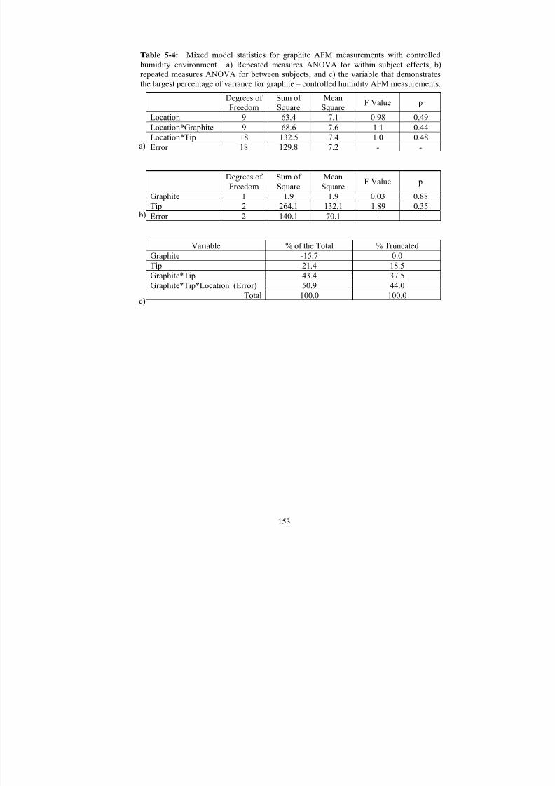
7/27/2019 Atomic Force Microscopy Method Development for Surface Energy Analysis
http://slidepdf.com/reader/full/atomic-force-microscopy-method-development-for-surface-energy-analysis 175/365
153
Table 5-4: Mixed model statistics for graphite AFM measurements with controlledhumidity environment. a) Repeated measures ANOVA for within subject effects, b)repeated measures ANOVA for between subjects, and c) the variable that demonstratesthe largest percentage of variance for graphite – controlled humidity AFM measurements.
Degrees of
Freedom
Sum of
Square
Mean
Square F Value pLocation 9 63.4 7.1 0.98 0.49Location*Graphite 9 68.6 7.6 1.1 0.44Location*Tip 18 132.5 7.4 1.0 0.48Error 18 129.8 7.2 - -
Degrees of Freedom
Sum of Square
MeanSquare
F Value p
Graphite 1 1.9 1.9 0.03 0.88Tip 2 264.1 132.1 1.89 0.35Error 2 140.1 70.1 - -
Variable % of the Total % TruncatedGraphite -15.7 0.0Tip 21.4 18.5Graphite*Tip 43.4 37.5Graphite*Tip*Location (Error) 50.9 44.0
Total 100.0 100.0
a)
b)
c)

7/27/2019 Atomic Force Microscopy Method Development for Surface Energy Analysis
http://slidepdf.com/reader/full/atomic-force-microscopy-method-development-for-surface-energy-analysis 176/365
154
Figure 5-1: The force, work, and surface energy of a) graphite measured in ambientconditions and b) graphite measured in controlled humidity conditions. The averages andstandard deviations are listed next to each histogram.
Average = 16.5 ± 1.7 nN
Average = 81.8 ± 6.8 mN/m
Average = 38.5 ± 5.9 mJ/m2
Average = 12.9 ± 1.4 nN
Average = 65.8 ± 5.2 mN/m
Average = 34.8 ± 4.8 mJ/m2 b)
a)

7/27/2019 Atomic Force Microscopy Method Development for Surface Energy Analysis
http://slidepdf.com/reader/full/atomic-force-microscopy-method-development-for-surface-energy-analysis 177/365
155
Figure 5-2: Iterative calculation to determine the value of β and the surface-vapor term.

7/27/2019 Atomic Force Microscopy Method Development for Surface Energy Analysis
http://slidepdf.com/reader/full/atomic-force-microscopy-method-development-for-surface-energy-analysis 178/365
156
Figure 5-3: Iterative calculation to illustrate how the value of β and the surface-vapor term are determined.

7/27/2019 Atomic Force Microscopy Method Development for Surface Energy Analysis
http://slidepdf.com/reader/full/atomic-force-microscopy-method-development-for-surface-energy-analysis 179/365
157
5.1.1.2 Mica Ambient and Controlled RH Solid-Vapor Surface Energy
The same flow diagram (Figure 4-4, surface energy model 2 and 3) was followed for
calculating solid-vapor surface energy of mica in ambient and controlled conditions. The
tip radius and tip-vapor surface energy for each tip used with the mica measurements are
reported in Table 5-5. These values were used to calculate the solid-vapor surface
energy using equations for surface energy models 2 and 3.
In order to calculate an average surface energy using the data from different tips and
samples, the repeated measures mixed model is applied to the force data of mica. The
variance within the subjects and between the subjects for the ambient measurements is
reported in Table 5-6a and b, and in Table 5-7a and b for controlled environment
measurements. The results for both ambient and controlled humidity illustrated that the
variation between the locations, the samples, and the tips was similar, because the p
values were greater than 0.05. Thus, the null hypothesis was accepted, and an average
force, work, and surface energy for the ambient and controlled environments could be
calculated. The results for ambient and controlled humidity are shown in Figure 5-4a
and Figure 5-4b. The variable that caused the largest error in ambient and controlled
humidity is shown in Table 5-6c and Table 5-7c. In ambient measurements, the largest
variation was due to the mica-tip interaction and the overall error within the
measurements. In controlled environment measurements, the largest variation was from
the mica*tip interaction and the overall error within the measurements. Controlled
humidity can sometimes cause tribocharging or electrostatic forces.[58] The biggest
concern with electrostatic forces would be on the surface of graphite, since mica is not
conductive. Attempts to produce an STM image failed because mica does not carry a

7/27/2019 Atomic Force Microscopy Method Development for Surface Energy Analysis
http://slidepdf.com/reader/full/atomic-force-microscopy-method-development-for-surface-energy-analysis 180/365
158
charge. Thus, tribocharging was likely not contributing to the variability. The best way
to eliminate electrostatic forces was to increase the humidity. However, the average
forces on mica in ambient and controlled humidity were different. This indicated a
strong capillary effect with mica, and increasing the humidity could introduce too many
force variations. Since the p values were well above 0.05, the variability was not causing
major problems for measurements between the tip and mica.
The average solid-vapor surface energy for mica in ambient and controlled environmental
conditions, as determined using models 2 and 3, is reported in Table 5-8. The pull-off
forces decreased when the relative humidity was low and the sample was allowed to sit in
the desiccator for 24 hours. Since both the tip and mica are hydrophilic, the large
difference between ambient and controlled environment forces was expected. In the
controlled humidity measurements, water adsorption to the surface of the mica sample
was significantly reduced, if not eliminated entirely. The removal of water eliminated the
capillary forces present when the relative humidity was high. The water on the surface
strongly interacted with mica and the tip making it difficult to pull the tip from the
surface. These results illustrate the importance of measuring forces with the AFM in a
controlled environment, especially with hydrophilic surfaces.
To evaluate the effectiveness of the AFM in determining surface energy, results were
compared to contact angle solid-vapor surface energy. The contact angle and AFM
results are listed in Table 5-8. The solid-vapor surface energy of mica in ambient
conditions was comparable with the van Oss model obtained using contact angle
measurements. The solid-vapor surface energy measured in a controlled environment
was less then the contact angle solid-vapor surface energy. Due to the disparity in the

7/27/2019 Atomic Force Microscopy Method Development for Surface Energy Analysis
http://slidepdf.com/reader/full/atomic-force-microscopy-method-development-for-surface-energy-analysis 181/365
159
contact angle models, it was difficult to compare the results from the AFM. The contact
angle method relied on measuring angles of liquids with various surface tensions and
fitting them to models based on the geometric mean. Each of these models used different
ways to incorporate the polar or acid/base term, and the results in Chapter 2 showed how
significantly this term varied. The ambient AFM and contact angle determined solid-
vapor surface energies were measured in uncontrolled conditions. Therefore, water vapor
that settled on samples during contact angle measurements affected the spread of the
liquids during contact angle measurements. Water vapor adsorbed on the surface of mica
in ambient conditions also contributed to large pull-off forces with the AFM. For hydrophilic surfaces, the water adsorbed to the surface limited the ability for direct
comparison between the AFM surface energy and the contact angle determined surface
energy. For mica, controlled environment conditions most likely report the “true” solid-
vapor surface energy.
Lastly, the surface energy models were evaluated. The results in Table 5-8 indicate the
calculated surface energy from the geometric mean (model 2) and the modified geometric
mean (model 3) were similar. The ambient solid-vapor surface energy was 45.0 mJ/m2
and 44.9 mJ/m2 for model 2 and model 3, respectively. The controlled environment
solid-vapor surface energy was 30.6 mJ/m2 and 30.8 mJ/m2 for model 2 and model 3.
The modification added in model 3 indicated that the geometric mean did not
overestimate the mica solid-vapor surface energy. Therefore, the solid-vapor surface
energy results shown in Figure 5-4 were calculated based on model 2. In model 3, the
assumption was made that the contact angle determined empirical β value could be used
with the AFM. As part of the analysis in Matlab, iterations were performed using the β

7/27/2019 Atomic Force Microscopy Method Development for Surface Energy Analysis
http://slidepdf.com/reader/full/atomic-force-microscopy-method-development-for-surface-energy-analysis 182/365
160
determined by Neumann's lab to determine solid-vapor surface energy. During these
iterations, the Matlab program also determined an optimized the β value as previously
discussed. The optimized β value was five times smaller than the empirical value
determined in the Neumann lab.[59]

7/27/2019 Atomic Force Microscopy Method Development for Surface Energy Analysis
http://slidepdf.com/reader/full/atomic-force-microscopy-method-development-for-surface-energy-analysis 183/365
161
Table 5-5: Tip radius and average tip-vapor surface energy (standard deviation) for thetips used to calculate the solid-vapor surface energy of mica in ambient and controlledhumidity environments.
TipEnvironmental
Conditions
Radius
(nm)
Force
(nN)
Work
(mN/m)
SurfaceEnergy
(mJ/m2)
1 Ambient 43 19.0 (8.9) 93.7 (8.9) 46.9 (8.9)
2 Ambient 41 17.4 (6.2) 89.9 (6.2) 45 (6.2)
3 Ambient 44 18.8 (2.6) 90.5 (2.6) 45.2 (2.6)
4 ControlledHumidity 44 12.5 (0.8) 60.4 (3.7) 30.2 (1.8)
5ControlledHumidity
43 12.9 (0.6) 63.6 (2.9) 31.8 (1.5)
6ControlledHumidity
40 10.9 (0.5) 57.9 (2.6) 29.0 (1.3)

7/27/2019 Atomic Force Microscopy Method Development for Surface Energy Analysis
http://slidepdf.com/reader/full/atomic-force-microscopy-method-development-for-surface-energy-analysis 184/365
162
Table 5-6: Mixed model statistics for mica AFM measurements in ambientenvironmental conditions. a) Repeated measures ANOVA for within subject effects, b)repeated measures ANOVA for between subjects, and c) the variable that demonstratesthe largest percentage of variance for mica – ambient AFM measurements.
Degrees of Freedom Sum of Square MeanSquare F Value p
Location 9 18.6 2.1 0.42 0.91Location*Mica 9 70.1 7.8 1.57 0.20Location*Tip 18 167.7 9.31 1.87 0.10Error 18 89.5 5.0 - -
Degrees of Freedom
Sum of Square
MeanSquare
F Value p
Mica 1 71.3 71.3 1.07 0.41
Tip 2 58.3 29.1 0.44 0.70Error 2 133.5 66.7 - -
Variable % of the Total % TruncatedMica 1.3 1.1Tip -16.4 0.0Mica*Tip 51.7 44.5Mica*Tip*Location (Error) 63.3 54.4
Total 100.0 100.0
a)
c)
b)

7/27/2019 Atomic Force Microscopy Method Development for Surface Energy Analysis
http://slidepdf.com/reader/full/atomic-force-microscopy-method-development-for-surface-energy-analysis 185/365
163
Table 5-7: Mixed model statistics for mica AFM measurements in controlled humidityenvironmental conditions. a) Repeated measures ANOVA for within subject effects, b)repeated measures ANOVA for between subjects, and c) the variable that demonstratesthe largest percentage of variance for mica – controlled AFM measurements.
Degrees of
Freedom
Sum of
Square
Mean
Square F Value pLocation 9 12.1 1.4 1.26 0.38Location*Mica 9 4.1 0.5 0.43 0.90Location*Tip 18 20.2 1.1 1.05 0.46Error 18 19.3 1.1 - -
Degrees of Freedom
Sum of Square
MeanSquare
F Value p
Mica 1 6.7 6.7 0.17 0.72Tip 2 3.6 1.8 0.05 0.96Error 2 76.7 38.3 - -
Variable % of the Total % TruncatedMica -57.9 0.0Tip -100.1 0.0Mica*Tip 204.8 79.4Mica*Tip*Location (Error) 53.2 20.6
Total 100.0 100.0
a)
c)
b)

7/27/2019 Atomic Force Microscopy Method Development for Surface Energy Analysis
http://slidepdf.com/reader/full/atomic-force-microscopy-method-development-for-surface-energy-analysis 186/365
164
Figure 5-4: The force, work, and surface energy of a) mica measured in ambientconditions and b) mica measured in controlled humidity conditions. The averages andstandard deviations are listed next to each histogram.
Average = 18.5 ± 0.9 nN
Average = 90.2 ± 4.6 mN/m
Average = 45.0 ± 4.1 mJ/m2
Average = 12.6 ± 0.2 nN
Average = 61.3 ± 0.9 mN/m
Average = 30.6 ± 0.9 mJ/m2
a)
b)

7/27/2019 Atomic Force Microscopy Method Development for Surface Energy Analysis
http://slidepdf.com/reader/full/atomic-force-microscopy-method-development-for-surface-energy-analysis 187/365
165
Table 5-8: Average solid-vapor surface energy of mica determined using the AFM andcontact angle methods.
Solid-Vapor Surface Energy (mJ/m2)
Method Indirect Model
Ambient
ForceMeasurements
Controlled RH
ForceMeasurements
Model 1 - -
Model 2 45.0 (4.1) 30.6 (0.9)
Model 3 44.9 (4.1) 30.8 (1.9)AFM
Model 4 - -
Van Oss et al 41.3 (2.7) NA
OWRK 65.2 (0.3) NACA
Neumann 57.0 (0.4) NA

7/27/2019 Atomic Force Microscopy Method Development for Surface Energy Analysis
http://slidepdf.com/reader/full/atomic-force-microscopy-method-development-for-surface-energy-analysis 188/365
166
The graphite solid-vapor surface energy from the AFM measurements was comparable to
the solid-vapor surface energy from contact angle measurements. The mica solid vapor
surface energy was difficult to compare because of the limitation with the indirect contact
angle models, though this was not the only reason for the disparity. Since liquids were
needed, uncertainties invariably exist because the thermodynamically equilibrated
condition can never be satisfied. However, the AFM did not rely on several extraneous
parameters to determine surface energy, and forces were measured in a controlled
humidity environment. The two models proved to be effective for use with the AFM.
With these results, the next objective was to evaluate solid-liquid surface energies.
5.1.2 Solid-liquid surface energy
The second part in evaluating the AFM’s potential for measuring surface energy involved
taking force measurements in liquid environments. With certain hygroscopic liquids
more variability existed in the force measurements than with water and diiodomethane.
Therefore, ethylene glycol and formamide were purified before use and rehydrated to
evaluate the effect water had on the AFM measurements in those liquids. In this section,
a similar presentation of data will be given. Since the solid-liquid surface energy could
be calculated using all four models, refer to the the flow diagrams previously presented in
Chapter 4.
5.1.2.1 Water Solid-Liquid Surface Energy
To determine the solid-liquid surface energy of mica and graphite in water, the spring
constant, tip radii, and tip-liquidwater surface energies had to first be determined. The
spring constant was measured in water because the oscillations of the cantilever were
different in air and in liquid. The same thermal method was used as described in Section

7/27/2019 Atomic Force Microscopy Method Development for Surface Energy Analysis
http://slidepdf.com/reader/full/atomic-force-microscopy-method-development-for-surface-energy-analysis 189/365
167
3.3. Table 5-9 shows the spring constant, radii, and other values used to calculate mica
and graphite solid-liquidwater surface energy.
Statistical analysis was performed on the AFM force data from graphite-water. Table
5-10a and b show the results from the SAS analysis. The p values indicate that the null
hypothesis was accepted. The analysis within subjects (Table 5-10a) for
graphite*locations had a low p value, slightly larger than the requisite 0.05 necessary to
indicate that the differences in the locations within the graphite samples are close to being
statistically significant. Since graphite is hydrophobic, more variability between
locations could have been due to the material's aversion to water. The graphite quality
could have also contributed to the variability. Of the three possible grades of HOPG, the
lowest grade was used in these studies, resulting in more steps during cleavage. Thus, the
combination of surface roughness and hydrophobicity of graphite can cause variations in
the locations. The analysis between subjects (Table 5-10b) for tips had a low p value
that was just above 0.05, and therefore, the differences between tips are almost
statistically significant. Again, the hydrophobicity of graphite was a major contributor to
variation. Even though the statistics can uncover these differences, the scientific
understanding of the weak interaction between water and graphite helps draw the
appropriate conclusions. In this study, the JMP output in Table 5-10c can be used to
verify the decision to accept the null hypothesis. Even though some variability was
caused by the tips, the largest error was attributed to the residual error, which is just the
experimental error of the measurements.
The graphite-water averages for force, work, and surface energy are plotted in Figure
5-5. The force of adhesion between graphite-water was large because the two are not
7/27/2019 Atomic Force Microscopy Method Development for Surface Energy Analysis
http://slidepdf.com/reader/full/atomic-force-microscopy-method-development-for-surface-energy-analysis 190/365

7/27/2019 Atomic Force Microscopy Method Development for Surface Energy Analysis
http://slidepdf.com/reader/full/atomic-force-microscopy-method-development-for-surface-energy-analysis 191/365
169
Waals interactions. Thus, a modification to the geometric mean might not be necessary
when evaluating samples with strong van der Waals forces.

7/27/2019 Atomic Force Microscopy Method Development for Surface Energy Analysis
http://slidepdf.com/reader/full/atomic-force-microscopy-method-development-for-surface-energy-analysis 192/365
170
Table 5-9: Spring constant, tip radius, and average tip-liquid surface energy (standarddeviation) are listed for the AFM tips used to measure the solid-liquid surface energy of graphite and mica in water.
Tip Material
Spring
constant(N/m)
Radius(nm)
Force(nN)
Work (mN/m)
Tip-Liquid
SurfaceEnergy
(mJ/m2)
1 43 1.2 (0.2) 6.0 (1.2) 3.0 (0.6)
2 41 1.1 (0.3) 5.7 (1.6) 2.8 (0.8)
3
Mica
42 1.0 (0.6) 5.3 (3.0) 2.6 (1.5)
1 41 0.9 (0.2) 4.5 (1.3) 2.3 (0.7)
2 43 1.0 (0.2) 4.9 (1.0) 2.5 (0.5)
3
Graphite
.04
42 0.8 (0.5) 4.0 (2.3) 2.0 (1.2)

7/27/2019 Atomic Force Microscopy Method Development for Surface Energy Analysis
http://slidepdf.com/reader/full/atomic-force-microscopy-method-development-for-surface-energy-analysis 193/365
171
Table 5-10: Mixed model statistics for graphite AFM measurements with water. a)Repeated measures ANOVA for within subject effects, b) repeated measures ANOVA for between subjects, and c) the variable that demonstrates the largest percentage of variancefor graphite – water AFM measurements.
Degrees of
Freedom
Sum of
Square
Mean
Square F Value pLocation 9 12.7 1.4 0.19 0.99Location*Graphite 9 155.0 17.2 2.31 0.07Location*Tip 18 85.5 4.8 0.64 0.82Error 18 134.4 7.5 - -
Degrees of Freedom
Sum of Square
MeanSquare
F Value p
Graphite 1 9.4 9.4 2.18 0.28Tip 2 118.8 59.4 13.8 0.07Error 2 8.7 4.3 - -
Variable % of the Total % TruncatedGraphite 1.6 1.5Tip 25.4 24.5Graphite*Tip -3.7 0.0Graphite*Tip*Location (Error) 76.7 74.0
Total 100.0 100.0
a)
b)
c)

7/27/2019 Atomic Force Microscopy Method Development for Surface Energy Analysis
http://slidepdf.com/reader/full/atomic-force-microscopy-method-development-for-surface-energy-analysis 194/365
172
Figure 5-5: The force, work, and surface energy of graphite measured in water. Theaverages and standard deviations are listed next to each histogram.
Average = 3.3 ± 0.4 nN
Average = 16.8 ± 2.0 mN/m
Average = 31.8 ± 7.4 mJ/m2
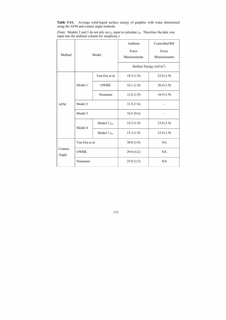
7/27/2019 Atomic Force Microscopy Method Development for Surface Energy Analysis
http://slidepdf.com/reader/full/atomic-force-microscopy-method-development-for-surface-energy-analysis 195/365
173
Table 5-11: Average solid-liquid surface energy of graphite with water determinedusing the AFM and contact angle methods.
(Note: Models 2 and 3 do not rely on γsv input to calculate γsl. Therefore the data wasinput into the ambient column for simplicity.)
Ambient
Force
Measurements
Controlled RH
Force
MeasurementsMethod Model
Surface Energy (mJ/m2)
Van Oss et al 18.5 (1.9) 22.8 (1.9)
OWRK 16.1 (1.9) 20.4 (1.9)Model 1
Neumann 12.6 (1.9) 16.9 (1.9)
Model 2 31.8 (7.4) -
Model 3 34.5 (9.6) -
Model 2 γsv 14.3 (1.9) 15.0 (1.9)
AFM
Model 4
Model 3 γsv 15.3 (1.9) 15.4 (1.9)
Van Oss et al 30.0 (3.9) NA
OWRK 29.0 (4.2) NAContact
Angle
Neumann 25.0 (3.5) NA

7/27/2019 Atomic Force Microscopy Method Development for Surface Energy Analysis
http://slidepdf.com/reader/full/atomic-force-microscopy-method-development-for-surface-energy-analysis 196/365
174
The second statistical analysis was done with the mica-water measurements. Table
5-12a and Table 5-12b give the SAS output for the analysis within subjects and between
subjects. The statistical analysis for mica does not calculate any p values less than 0.05
and the null hypothesis was accepted. Table 5-12c captures the JMP output for the
factors that contributed to variation while studying the interactions between mica and
water. These results showed the majority of the variation was residual error, with a small
portion attributed to tip variability. However, the SAS data did not indicate that any
variability would invalidate the null hypothesis. Therefore, an average force, work, and
surface energy data could be calculated (see Figure 5-6).
The average force of adhesion for mica, illustrated in Figure 5-6, was smaller compared
to that of graphite. The smaller force value indicated mica's affinity for water. Similarly,
the measured contact angle on mica was 10.0 ± 2.4, therefore, the water completely
spread over the surface of mica. A strong interaction of water with mica meant the solid-
liquid surface energy would also be small. The calculated solid-liquid surface energies
from all four AFM models and contact angle are given in Table 5-13. Unfortunately, a
direct comparison could not be made between AFM solid-liquid surface energy and
contact angle solid-liquid surface energy because of the limitations with the indirect
models used with contact angle measurements. Contact angles use Young's equation to
balances the forces to determine solid-liquid surface energy. In some instances, negative
solid-liquid surface energy values were obtained. These values did not have a physical
meaning and make it challenging to evaluate the capabilities of the AFM. Scientifically,
from contact angle measurements, one could suggest that the solid-liquid surface energy
of water would be smaller than the solid-liquid surface energy of ethylene glycol and

7/27/2019 Atomic Force Microscopy Method Development for Surface Energy Analysis
http://slidepdf.com/reader/full/atomic-force-microscopy-method-development-for-surface-energy-analysis 197/365
7/27/2019 Atomic Force Microscopy Method Development for Surface Energy Analysis
http://slidepdf.com/reader/full/atomic-force-microscopy-method-development-for-surface-energy-analysis 198/365
176
differences in electronic properties and molecular size were small. [21] Any large
differences and the geometric mean would overestimate surface energy, hence, the need
for the modification. The studies done with mica-water indicate the assumption was
valid.
Model 4 utilized only AFM data for the calculation of γsurface-tip. There were differences
in the AFM ambient and controlled γsolid-vapor surface energy (Table 5-8), but the solid-
liquid surface energy variations were minimized by the compensating effects of two
simultaneously changing variables. Without other reliable mica-water solid-liquid
surface energy values, it was undetermined which of models 2, 3, or 4 is better. Since
models 2 and 3 were equivalent, there was no need to go through a rigorous fitting,
especially since software was not available. Also, there was no indication which model
was better between model 2 and model 4. As mentioned, the overriding assumption for
model 2 was that the geometric mean can be used to describe the interaction of two
dissimilar materials as long as the component's differences in electronic properties and
molecular size were small. Since mica also has electron donating/accepting capabilities,
it was not certain that the geometric mean captured these interactions, despite model 2
and model 3 reporting the same result. The empirical correction factor in model 3 has not
been used outside of contact angle measurements and might not be applicable in fitting
the AFM data. Model 4 assumed that the surface was unchanged between vapor and
liquid measurements. Since the surface of mica was relatively inert, this assumption
might be valid. However, the assumption might not apply when using a crystalline
material. Therefore, models 2, 3, and 4 were all considered viable options for evaluating
hydrophilic surfaces.
7/27/2019 Atomic Force Microscopy Method Development for Surface Energy Analysis
http://slidepdf.com/reader/full/atomic-force-microscopy-method-development-for-surface-energy-analysis 199/365
177
Table 5-12: Mixed model statistics for mica AFM measurements with water. a)Repeated measures ANOVA for within subject effects, b) repeated measures ANOVA for between subjects, and c) the variable that demonstrates the largest percentage of variancefor mica – water AFM measurements.
Degrees of
Freedom
Sum of
Square
Mean
Square F Value pLocation 9 0.09 0.009 1.53 0.21Location*Mica 9 0.03 0.003 0.54 0.83Location*Tip 18 0.15 0.008 1.38 0.25Error 18 0.11 0.006 - -
Degrees of Freedom
Sum of Square
MeanSquare
F Value p
Mica 1 0.0007 0.0007 0.10 0.78Tip 2 0.0600 0.0300 4.12 0.19Error 2 0.0145 0.007 - -
Variable % of the Total % TruncatedMica -2.9 0.0Tip 15.1 14.7Mica*Tip 1.0 1.0Mica*Tip*Location (Error) 86.7 84.3
Total 100.0 100.0
a)
c)
b)

7/27/2019 Atomic Force Microscopy Method Development for Surface Energy Analysis
http://slidepdf.com/reader/full/atomic-force-microscopy-method-development-for-surface-energy-analysis 200/365
178
Figure 5-6: The force, work, and surface energy of mica measured in water. Theaverages and standard deviations are listed next to each histogram.
Average = 0.5 ± 0.1 nN
Average = 2.7 ± 0.5 mN/m
Average = 0.7 ± 0.2 mJ/m2

7/27/2019 Atomic Force Microscopy Method Development for Surface Energy Analysis
http://slidepdf.com/reader/full/atomic-force-microscopy-method-development-for-surface-energy-analysis 201/365
179
Table 5-13: Average solid-liquid surface energy of mica with water determined usingthe AFM and contact angle methods.
(Note: Models 2 and 3 do not rely on γsv input to calculate γsl. Therefore the data wasinput into the ambient column for simplicity.)
Ambient
Force
Measurements
Controlled RH
Force
MeasurementsMethod Model
Surface Energy (mJ/m2)
Van Oss et al -0.9 (1.1) 12.6 (1.1)
OWRK 23.0 (1.1) 36.5 (1.1)Model 1
Neumann 14.8 (1.1) 28.3 (1.1)
Model 2 0.7 (0.2) -
Model 3 0.7 (0.2) -
Model 2 γsv 2.8 (1.1) 1.9 (1.1)
AFM
Model 4
Model 3 γsv 2.6 (1.1) 2.4 (1.1)
Van Oss et al -31.1 (2.3) NA
OWRK -6.4 (0.5) NAContact
Angle
Neumann -14.7 (0.6) NA

7/27/2019 Atomic Force Microscopy Method Development for Surface Energy Analysis
http://slidepdf.com/reader/full/atomic-force-microscopy-method-development-for-surface-energy-analysis 202/365

7/27/2019 Atomic Force Microscopy Method Development for Surface Energy Analysis
http://slidepdf.com/reader/full/atomic-force-microscopy-method-development-for-surface-energy-analysis 203/365
181
challenging to compare the results of the contact angle measurements to the AFM data
because of the indirect models and Young's equation. One negative number was
observed from the diiodomethane measurements; therefore, the range of solid-liquid
surface energies was (-3.5 to 0.7 mJ/m2). However, the AFM results could be compared
to the OWRK and van Oss contact angle models. The solid-liquid surface energy for
AFM model 1 using γst determined from van Oss and OWRK contact angle model was
relatively low. Thus, there were two reasons for avoiding the use of model 1. First, the
solid-liquid surface energy determined by the other AFM models was smaller, and as a
result, comparable to contact angle results. Second, requiring a combination of two
surface energy methods suggested the AFM was not an adequate instrument for
evaluating surface energy. Therefore, model 1 was still not the optimal choice for the
AFM. Model 2 and 3 were similar in solid-liquid surface energy and also comparable to
the contact angle OWRK solid-liquid surface energy. These two models continued to
show applicability with the AFM and surfaces with van der Waals forces. Also, since the
γsl and γtl were similar, the modification did not show differences when the solid-liquid
surface energy was calculated. Model 4 was also successfully compared to contact angle
data. Ambient and controlled humidity solid-liquid surface energies were not
significantly different because the γsolid-vapor for graphite in ambient and controlled
environment were also not significantly different (Table 5-2). Therefore, model 4 could
be used. In the previous section, discussion of mica-water solid-liquid surface energy
compared the advantages and disadvantages of using models 2, 3, and 4. In studies with
inert surfaces, the γsurface-tip may be unchanged between vapor and liquid measurements;

7/27/2019 Atomic Force Microscopy Method Development for Surface Energy Analysis
http://slidepdf.com/reader/full/atomic-force-microscopy-method-development-for-surface-energy-analysis 204/365
182
however, it is cautioned that this may not be the case for crystalline material. However,
consideration will be given to these models when calculating solid-liquid surface energy.

7/27/2019 Atomic Force Microscopy Method Development for Surface Energy Analysis
http://slidepdf.com/reader/full/atomic-force-microscopy-method-development-for-surface-energy-analysis 205/365
183
Table 5-14: Spring constant, tip radius, and average tip-liquid surface energy (standarddeviation) are listed for the AFM tips used to measure the solid-liquid surface energy of graphite and mica in diiodomethane.
Tip Material
Spring
constant(N/m)
Radius
(nm)
Force
(nN)
Work
(mN/m)
Surface
Energy(mJ/m2)
1 45 0.8 (0.1) 3.8 (0.5) 1.9 (0.2)
2 43 0.9 (0.3) 4.7 (1.3) 2.3 (0.7)
3
Mica
42 0.8 (0.1) 4.1 (0.5) 2.1 (0.3)
1 42 0.8 (0.3) 4.1 (1.3) 2.1 (0.6)
2 43 0.8 (0.2) 3.7 (1.1) 1.9 (0.6)
3
Graphite
.04
43 0.9 (0.3) 4.6 (1.4) 2.3 (0.7)

7/27/2019 Atomic Force Microscopy Method Development for Surface Energy Analysis
http://slidepdf.com/reader/full/atomic-force-microscopy-method-development-for-surface-energy-analysis 206/365
184
Table 5-15: Mixed model statistics for graphite AFM measurements withdiiodomethane. a) Repeated measures ANOVA for within subject effects, b) repeatedmeasures ANOVA for between subjects, and c) the variable that demonstrates the largest percentage of variance for graphite – diiodomethane AFM measurements.
Degrees of
Freedom
Sum of
Square
Mean
Square F Value pLocation 9 0.29 0.03 1.45 0.24Location*Graphite 9 0.24 0.03 1.19 0.36Location*Tip 18 0.60 0.03 1.50 0.20Error 18 0.40 0.02 - -
Degrees of Freedom
Sum of Square
MeanSquare
F Value p
Graphite 1 0.02 0.024 3.00 0.23Tip 2 0.26 0.129 16.08 0.06Error 2 0.02 0.008 - -
Variable % of the Total % TruncatedGraphite 1.7 1.6Tip 18.8 17.7Graphite*Tip -6.1 0.0Graphite*Tip*Location (Error) 85.7 80.7
Total 100.0 100.0
a)
b)
c)

7/27/2019 Atomic Force Microscopy Method Development for Surface Energy Analysis
http://slidepdf.com/reader/full/atomic-force-microscopy-method-development-for-surface-energy-analysis 207/365
185
Figure 5-7: The force, work, and surface energy of graphite-diiodomethane. Theaverages and standard deviations are listed next to each histogram.
b)
Average = 1.6 ± 0.8 mJ/m2
Average = 3.5 ± 1.0 mN/m
Average = 0.7 ± 0.2 nN

7/27/2019 Atomic Force Microscopy Method Development for Surface Energy Analysis
http://slidepdf.com/reader/full/atomic-force-microscopy-method-development-for-surface-energy-analysis 208/365
186
Table 5-16: Average solid-liquid surface energy of graphite with diiodomethanedetermined using the AFM and contact angle methods.
(Note: Models 2 and 3 do not rely on γsv input to calculate γsl. Therefore the data wasinput into the ambient column for simplicity.)
Ambient
Force
Measurements
Controlled RH
Force
MeasurementsMethod Model
Surface Energy (mJ/m2)
Van Oss et al 5.3 (0.9) 9.7 (0.9)
OWRK 2.9 (0.9) 7.3 (0.9)Model 1
Neumann -0.6 (0.9) 3.8 (0.9)
Model 2 1.6 (0.8) -
Model 3 1.6 (0.8) -
Model 2 γsv 1.1 (0.9) 1.8 (0.9)
AFM
Model 4
Model 3 γsv 1.1 (0.9) 1.8 (0.9)
Van Oss et al 0.6 (0.1) NA
OWRK 0.7 (0.9) NAContact
Angle
Neumann -3.3 (1.6) NA

7/27/2019 Atomic Force Microscopy Method Development for Surface Energy Analysis
http://slidepdf.com/reader/full/atomic-force-microscopy-method-development-for-surface-energy-analysis 209/365
187
Next, statistical analysis was done with the mica-diiodomethane measurements. The
SAS output in Table 5-17a and Table 5-17b for the analysis within subjects and between
subjects indicates that all p values were greater than 0.05; therefore, the null hypothesis
was accepted. Table 5-17c gives the JMP output for the contributing factors of variation
in the study of mica-diiodomethane interaction. These results showed the majority of the
variation was residual error, while a small portion of error was attributed to the tips and
the mica samples. The variability between mica samples and tips could have been caused
by a less favorable interaction with diiodomethane. Mica did not have the same cleavage
difficulties associated with graphite; therefore, few to no steps form during the removalof a layer of mica. Like the mica-water statistical analysis, the SAS data did not indicate
that any variability would invalidate the null hypothesis. Therefore, an average force,
work, and surface energy data could be calculated (Figure 5-8).
The average force of adhesion for mica, illustrated in Figure 5-8, was larger compared to
that of graphite-diiodomethane. The large force value indicated that mica's interaction
with diiodomethane was less than that of graphite-diiodomethane. Similarly, the
measured contact angle on mica was 41.0 ± 2.9; therefore, the spread of diiodomethane
was less than the spread of water on mica. A weak interaction of diiodomethane with
mica meant the solid-liquid surface energy would be large. The calculated solid-liquid
surface energies from all four AFM models and contact angle are given in Table 5-18.
As discussed in the mica-water surface energy section, because of contact angle
limitations, a direct comparison cannot be made with the AFM and contact angle data. In
this study, contact angle solid-liquid surface energy values ranged from 0.8 to 26.9
mJ/m2. Scientifically, solid-liquid surface energy of diiodomethane should be larger than

7/27/2019 Atomic Force Microscopy Method Development for Surface Energy Analysis
http://slidepdf.com/reader/full/atomic-force-microscopy-method-development-for-surface-energy-analysis 210/365
188
the solid-liquid surface energy of ethylene glycol and water, which was verified by the
measured contact angles and the forces presented in this chapter. However, the
variability of the contact angle solid-vapor surface energies of mica (41.3 – 65.2 mJ/m2)
made it relatively impossible to unequivocally determine an average AFM solid-liquid
surface energy and the best AFM model. This is illustrated further in the values shown in
Table 5-18.
Although the AFM data for one model cannot be compared to the contact angle results,
the applicability of the AFM models will be evaluated. For model 1, the solid-liquid
surface energy values ranged from 5.1 to 42.5 mJ/m2. The range was a reflection of the
large contact angle solid-vapor surface energy range mentioned above. Therefore, model
1 was not considered because of the level of complexity added from discrepancies in
contact angle indirect models. The indirect models and Young's equation limited
comparison of the AFM results for a hydrophilic surface.
Models 2 and 3 were independent of contact measurements. The results from these two
models were similar and fell between the contact angle surface energy ranges. Since the
true value of mica-diiodomethane γsl was unclear from contact angle measurements, the
assumptions may have been invalid. So far the geometric mean and modified geometric
mean have proven useful for graphite-water and graphite-diiodomethane surface energy.
However, graphite had mostly van der Waals forces contributing to the overall surface
energy. Therefore, using a geometric mean model to calculate surface energy was
acceptable. The geometric mean, when applied to mica-ambient measurements, did show
agreement with one of the contact angle results. Since the variability was so large with
contact angle solid-vapor surface energy, it could not serve as the only justification

7/27/2019 Atomic Force Microscopy Method Development for Surface Energy Analysis
http://slidepdf.com/reader/full/atomic-force-microscopy-method-development-for-surface-energy-analysis 211/365

7/27/2019 Atomic Force Microscopy Method Development for Surface Energy Analysis
http://slidepdf.com/reader/full/atomic-force-microscopy-method-development-for-surface-energy-analysis 212/365
190
Table 5-17: Mixed model statistics for mica AFM measurements with diiodomethane.a) Repeated measures ANOVA for within subject effects, b) repeated measures ANOVAfor between subjects, and c) the variable that demonstrates the largest percentage of variance for mica – diiodomethane AFM measurements.
Degrees of
Freedom
Sum of
Square
Mean
Square F Value pLocation 9 16.1 1.8 1.48 0.23Location*Mica 9 12.7 1.4 1.17 0.37Location*Tip 18 34.7 1.9 1.60 0.16Error 18 21.7 1.2 - -
Degrees of Freedom
Sum of Square
MeanSquare
F Value p
Mica 1 12.3 12.3 3.27 0.21Tip 2 0.4 0.2 0.06 0.95Error 2 7.5 3.8 - -
Variable % of the Total % TruncatedMica 15.3 14.0Tip -9.5 0.0Mica*Tip 12.0 10.9Mica*Tip*Location (Error) 82.3 75.1
Total 15.3 14.0
a)
b)
c)

7/27/2019 Atomic Force Microscopy Method Development for Surface Energy Analysis
http://slidepdf.com/reader/full/atomic-force-microscopy-method-development-for-surface-energy-analysis 213/365
191
Figure 5-8: The force, work, and surface energy of mica-diiodomethane. The averagesand standard deviations are listed next to each histogram.
Average = 2.1 ± 0.3 nN
Average = 10.3 ± 1.3 mN/m
Average = 12.9 ± 3.1 mJ/m2

7/27/2019 Atomic Force Microscopy Method Development for Surface Energy Analysis
http://slidepdf.com/reader/full/atomic-force-microscopy-method-development-for-surface-energy-analysis 214/365
192
Table 5-18: Average solid-liquid surface energy of mica with diiodomethane determinedusing the AFM and contact angle methods.
(Note: Models 2 and 3 do not rely on γsv input to calculate γsl. Therefore the data wasinput into the ambient column for simplicity.)
Ambient
Force
Measurements
Controlled RH
Force
MeasurementsMethod Model
Surface Energy (mJ/m2)
Van Oss et al 5.1 (1.5) 18.6 (1.5)
OWRK 29.0 (1.5) 42.5 (1.5)Model 1
Neumann 20.8 (1.5) 34.3 (1.5)
Model 2 12.9 (3.1) -
Model 3 13.6 (4.3) -
Model 2 γsv 8.8 (1.5) 7.9 (1.5)
AFM
Model 4
Model 3 γsv 8.6 (1.5) 8.4 (1.5)
Van Oss et al 0.8 (0.2) NA
OWRK 26.9 (0.4) NAContact
Angle
Neumann 18.7 (1.7) NA

7/27/2019 Atomic Force Microscopy Method Development for Surface Energy Analysis
http://slidepdf.com/reader/full/atomic-force-microscopy-method-development-for-surface-energy-analysis 215/365
193
5.1.2.3 Formamide Solid-Liquid Surface Energy
The spring constant, tip radii, and tip-liquidformamidel surface energies were measured to
determine the solid-liquid surface energy of graphite in formamide. Table 5-19 shows
the values used to calculate graphite solid-liquidformamide surface energy.
Since formamide is a hygroscopic liquid, it was dried using distillation prior to use for
AFM and contact angle measurements. The dried liquid was then rehydrated to 0.5%,
1%, and 5% w/w water/formamide. The water amount was confirmed using Coulometric
Karl Fisher titration. Each liquid was used the day it was prepared.
Force measurements were made on graphite in formamide using the tips in Table 5-19.
Data analysis was performed in SAS and JMP. The statistics for dried, 0.5%, 1%, and
5% w/w water/formamide are listed in Table 5-20, Table 5-21, Table 5-22, and Table
5-23. From the statistics for graphite with dry, 0.5% w/w, and 1% w/w, and .5% w/w
water/formamide the null hypothesis was accepted and an average force, work, and
surface energy could be calculated. The plots of the these averages for graphite with dry
formamide, 0.5%, 1%, and 5% are shown in Figure 5-9, Figure 5-10, Figure 5-11, and
Figure 5-12.

7/27/2019 Atomic Force Microscopy Method Development for Surface Energy Analysis
http://slidepdf.com/reader/full/atomic-force-microscopy-method-development-for-surface-energy-analysis 216/365
194
Table 5-19: Tip radius and average tip-liquid surface energy (standard deviation) arelisted for the AFM tips used to measure the solid-liquid surface energy of graphite informamide. There are four conditions listed for formamide, dried, 0.5%, 1%, and 5%w/w water in formamide.
Tip Condition Springconstant
(N/m)
Radius(nm)
Force(nN)
Work (mN/m)
SurfaceEnergy
(mJ/m2)
1 41 0.6 (0.2) 3.0 (0.8) 1.5 (0.4)
2 40 0.6 (0.4) 2.9 (1.9) 1.4 (0.9)
3
Dry
41 0.5 (0.3) 2.6 (1.8) 1.3 (0.9)
1 41 0.6 (0.2) 3.3 (1.2) 1.7 (0.6)
2 40 0.8 (0.2) 4.1 (1.1) 2.1 (0.6)
3
0.5% w/w water
41 0.6 (0.2) 3.3 (0.8) 1.7 (0.4)
1 41 0.8 (0.2) 4.1 (1.1) 2.0 (0.6)
2 40 0.9 (0.3) 4.6 (1.6) 2.3 (0.8)
3
1% w/w water
41 0.9 (0.2) 4.5 (1.2) 2.2 (0.6)
1 41 0.7 (0.2) 3.8 (0.8) 1.9 (0.4)
2 40 0.8 (0.2) 4.3 (1.0) 2.2 (0.5)
3
5% w/w water
.05
41 0.9 (0.2) 4.8 (1.1) 2.4 (0.6)

7/27/2019 Atomic Force Microscopy Method Development for Surface Energy Analysis
http://slidepdf.com/reader/full/atomic-force-microscopy-method-development-for-surface-energy-analysis 217/365
195
The average force of adhesion from the AFM measurements increased with the increase
in water content in the formamide, demonstrating that moisture in the formamide had a
clear effect of the AFM measurements.
Fdry > F0.5% w/w > F1% w/w > F5%w/w
The solid-liquid surface energy of graphite-water was about 30 mJ/m2 and with 5% w/w
water added to formamide, the AFM calculated solid-liquid surface energy trended
towards the graphite-water solid-liquid surface energy. Thus, the AFM was extremely
sensitive to changes in liquid compositions. It is important to note that this is a limitation
of contact angles. In chapter 2, the problem of non-homogenous distribution of additives
at the three phases of contact angle measurements was discussed. These data from the
AFM demonstrated the instrument's ability to detect changes to a solvent and more
importantly, how the changes affect the interaction between the solvent and surface. The
data also showed the effect that water had on the variations in measurements. There was
an increase in the range of forces, which was exacerbated in the surface energy
calculations as the water in formamide increased from about 0% to 5% w/w
water/formamide. The variability was also evident in the JMP data, as shown in Table
5-20c, Table 5-21c ,Table 5-22c, and Table 5-23c. As the water increased, the cause of
variability started to shift from purely residual error of the measurements to large error in
graphite samples, tips, and the interaction between the sample and tip (Table 5-23c).
Therefore, it was important to ensure hygroscopic liquids were dried before use in AFM
measurements for a “true” surface energy value.
The force of adhesion measurements for dried formamide were expected to fall
somewhere between the measurements from diiodomethane and water since formamide

7/27/2019 Atomic Force Microscopy Method Development for Surface Energy Analysis
http://slidepdf.com/reader/full/atomic-force-microscopy-method-development-for-surface-energy-analysis 218/365
196
has polar and nonpolar components. Therefore, the surface energy would also project in
the middle. This was also observed in the contact angle measurements. The contact
angle measurement of dried formamide on graphite was 60.9 ± 2.4. The force of
adhesion from AFM measurements reflected the same. In Table 5-24, the graphite-dried
formamide solid-liquid surface energy is shown for AFM and contact angle
measurements. This was the first time that the choice of models was not straightforward.
The contact angle data gave a solid-liquid surface energy range of 8.7 to 13.7 mJ/m2 and
the range from the four AFM models is 5 to 15.2 mJ/m2.
Model 1 used the γsv from contact angle measurements to determine γst. Since the
graphite-ambient solid-vapor surface energy was only 4 mJ/m2 higher than the controlled
humidity solid-vapor surface energy, the difference between the solid-liquid surface
energies for model 1 was also small. Although the values were similar, the controlled
RH force calculated solid-liquid surface energy was closest to the corresponding contact
angle method. This was the first data set to have comparable results with contact angle
results. However, for the AFM to be a standalone instrument, it was still not
recommended to include other surface energy measurements into an AFM model.
Models 2 and 3, which use the geometric mean, calculated an average surface energy
equivalent to the van Oss contact angle solid-liquid surface energy. These models
consistently showed the best comparability between the AFM and contact angle results.
Since, graphite has mostly van der Waals forces; it satisfied the necessary assumptions
for a model developed for non-bonding interactions. Model 4 used the AFM γsv to
determine γst. Since γsv from the AFM measurements was smaller than the γsv of the
contact angle measurements, the γsl was also expected to be smaller. These results were

7/27/2019 Atomic Force Microscopy Method Development for Surface Energy Analysis
http://slidepdf.com/reader/full/atomic-force-microscopy-method-development-for-surface-energy-analysis 219/365
197
relatively comparable to the lower end of the contact angle results (Neumann model).
Compared to water and diiodomethane, formamide has both dispersive and polar
intramolecular forces. Water has more polar forces and diiodomethane has more
dispersive forces. From these results, it seemed that the liquid with both forces gave the
best and most consistent results from the all four models. The extremes, water and
diiodomethane, each seemed to have a few differences whether it’s from the limitations
of contact angle measurements or the inherent variability in the AFM measurements.
Formamide created more of an optimal condition for determining surface energy from
indirect models.
The average force of adhesion measurements made in rehydrated formamide increased
immediately even with only a 0.5% w/w increase in water content, causing the surface
energy to increase accordingly. The AFM and contact angle solid-liquid surface energy
are shown in Table 5-25. The contact angle for the 0.5% w/w water changed as well,
with the corresponding increase in solid-liquid surface energy. The contact angle solid-
liquid surface energy with 0.5% w/w water in formamide ranged from 11.7 to 18.2 mJ/m2
and from 7.6 to 19.8 mJ/m2 with AFM measurement The evaluation of the AFM models
for this liquid is the same as the results for dried formamide. Model 1solid-liquid surface
energy from the controlled RH γst, was comparable to the corresponding contact angle
models. Models 2 and 3 were comparable to the van Oss contact angle solid-liquid
surface energy, and model 4 was on the lower end of the range closer to the Neumann
contact angle solid-liquid surface energy. The change in force of adhesion and contact
angles with added water in formamide illustrates the importance of drying hygroscopic

7/27/2019 Atomic Force Microscopy Method Development for Surface Energy Analysis
http://slidepdf.com/reader/full/atomic-force-microscopy-method-development-for-surface-energy-analysis 220/365
198
liquids. The true solid-liquid surface energy between the solvent and sample's surface
cannot be found if the water is not removed.
The average force of adhesion measurements made in 1% w/w and 5% w/w
water/formamide continued to increase; subsequently causing the surface energy to
increase. The AFM and contact angle solid-liquid surface energy are shown for 1% and
5% w/w added water in Table 5-26 and Table 5-27. The contact angle with 1% w/w
water decreased (62.4 ± 3.8) as compared to the angle measured with 0.5% w/w water,
and then increased at 5% w/w water (64.3 ± 4.1). This lack of a clear trend illustrates
why additive solutions are not used with contact angle measurements. Since the contact
angles did not increase in the same manner as the AFM measurements, comparing the
solid-liquid surface energies became more challenging. For 1% w/w water in formamide,
model 1 (ambient measurements) and model 4 were most comparable. Model 1
(controlled RH), model 2, and model 3 were less comparable to the contact angle values
because the solid-liquid surface energy increased. It is hard to determine the validity of
the comparison because of the lack of confidence in the contact angle values with
mixtures. Similarly, for the 5% w/w water, model 1 (ambient measurements) and model
4 were more comparable to the contact angle solid-liquid surface energy, and model 1
(controlled RH), model 2, and model 3 were less comparable. The JMP statistics in
Table 5-22c and Table 5-23c for 1% and 5% w/w water/formamide also indicate that the
variability increased in the AFM measurements. The propagation of error through other
variables showed possible challenges with the AFM. These limitations might also have
been attributed to the use of a water mixture on a hydrophobic surface. The AFM is a
more sensitive instrument than the macroscopic sessile drop contact angles. Thus, the

7/27/2019 Atomic Force Microscopy Method Development for Surface Energy Analysis
http://slidepdf.com/reader/full/atomic-force-microscopy-method-development-for-surface-energy-analysis 221/365
199
spread and variability in the AFM measurements could be due to both formamide-
graphite and water-graphite interactions. To evaluate the AFM's ability to measure the
force of adhesion in a mixture solution, the next study was the investigation of the
hydrophilic surface of mica with dried and rehydrated ethylene glycol.

7/27/2019 Atomic Force Microscopy Method Development for Surface Energy Analysis
http://slidepdf.com/reader/full/atomic-force-microscopy-method-development-for-surface-energy-analysis 222/365
200
Table 5-20: Mixed model statistics for graphite AFM measurements with dryformamide. a) Repeated measures ANOVA for within subject effects, b) repeatedmeasures ANOVA for between subjects, and c) the variable that demonstrates the largest percentage of variance for graphite – dry formamide AFM measurements.
Degrees of
Freedom
Sum of
Square
Mean
Square F Value pLocation 9 16.4 1.8 0.87 0.56Location*Graphite 9 14.4 1.6 0.77 0.65Location*Tip 18 40.3 2.2 1.07 0.45Error 18 37.7 2.1 - -
Degrees of Freedom
Sum of Square
MeanSquare
F Value p
Graphite 1 4.8 4.8 2.33 0.27Tip 2 0.6 0.3 0.16 0.86Error 2 4.1 2.1 - -
Variable % of the Total % TruncatedGraphite 4.5 4.3Tip -4.2 0.0Graphite*Tip 0.1 0.0Graphite*Tip*Location (Error) 99.7 95.7
Total 100.0 100.0
a)
b)
c)
7/27/2019 Atomic Force Microscopy Method Development for Surface Energy Analysis
http://slidepdf.com/reader/full/atomic-force-microscopy-method-development-for-surface-energy-analysis 223/365
201
Table 5-21: Mixed model statistics for graphite AFM measurements with 0.5% w/wwater/formamide. a) Repeated measures ANOVA for within subject effects, b) repeatedmeasures ANOVA for between subjects, and c) the variable that demonstrates the largest percentage of variance for graphite – 0.5% w/w water/formamide AFM measurements.
Degrees of Freedom Sum of Square MeanSquare F Value p
Location 9 4.3 0.5 0.94 0.52Location*Graphite 9 3.6 0.4 0.80 0.62Location*Tip 18 9.4 0.5 1.04 0.47Error 18 9.1 0.5 - -
Degrees of Freedom
Sum of Square
MeanSquare
F Value p
Graphite 1 1.3 1.3 1.63 0.33
Tip 2 1.5 0.7 0.91 0.52Error 2 1.6 0.8 - -
Variable % of the Total % TruncatedGraphite -2.5 0.0Tip -4.7 0.0Graphite*Tip 5.9 5.5Graphite*Tip*Location (Error) 101.3 94.5
Total 100 100
a)
b)
c)

7/27/2019 Atomic Force Microscopy Method Development for Surface Energy Analysis
http://slidepdf.com/reader/full/atomic-force-microscopy-method-development-for-surface-energy-analysis 224/365
202
Table 5-22: Mixed model statistics for graphite AFM measurements with 1% w/wwater/formamide. a) Repeated measures ANOVA for within subject effects, b) repeatedmeasures ANOVA for between subjects, and c) the variable that demonstrates the largest percentage of variance for graphite – 1% w/w water/formamide AFM measurements.
Degrees of Freedom Sum of Square MeanSquare F Value p
Location 9 127.9 14.2 0.72 0.69Location*Graphite 9 134.9 15.0 0.76 0.66Location*Tip 18 497.3 27.6 1.39 0.24Error 18 356.6 19.8 - -
Degrees of Freedom
Sum of Square
MeanSquare
F Value p
Graphite 1 26.9 26.9 1.60 0.33
Tip 2 289.8 144.9 8.61 .10Error 2 33.7 16.8 - -
Variable % of the Total % TruncatedGraphite 1.2 1.2Tip 22.7 22.3Graphite*Tip -1.8 0.0Graphite*Tip*Location (Error) 77.9 76.5
Total 100.0 100.0
a)
b)
c)

7/27/2019 Atomic Force Microscopy Method Development for Surface Energy Analysis
http://slidepdf.com/reader/full/atomic-force-microscopy-method-development-for-surface-energy-analysis 225/365
203
Table 5-23: Mixed model statistics for graphite AFM measurements with 5% w/wwater/formamide. a) Repeated measures ANOVA for within subject effects, b) repeatedmeasures ANOVA for between subjects, and c) the variable that demonstrates the largest percentage of variance for graphite – 5% w/w water/formamide AFM measurements.
Degrees of Freedom Sum of Square MeanSquare F Value p
Location 9 106.6 11.8 0.85 0.59Location*Graphite 9 203.9 22.7 1.62 0.18Location*Tip 18 335.4 18.6 1.33 0.28Error 18 252.0 14.0 - -
Degrees of Freedom
Sum of Square
MeanSquare
F Value p
Graphite 1 138.9 138.9 3.11 0.22
Tip 2 202.3 101.2 2.27 0.31Error 2 89.2 44.6 - -
Variable % of the Total % TruncatedGraphite 12.0 12.0Tip 10.8 10.8Graphite*Tip 10.2 10.3Graphite*Tip*Location (Error) 67.0 67.0
Total 100.0 100.0
a)
b)
c)

7/27/2019 Atomic Force Microscopy Method Development for Surface Energy Analysis
http://slidepdf.com/reader/full/atomic-force-microscopy-method-development-for-surface-energy-analysis 226/365
204
Figure 5-9: The force, work, and surface energy of graphite-dried formamide. Theaverages and standard deviations are listed next to each histogram.
Average = 1.6 ± 0.2 nN
Average = 8.3 ± 1.0 mN/m
Average = 12.5 ± 2.9 mJ/m2
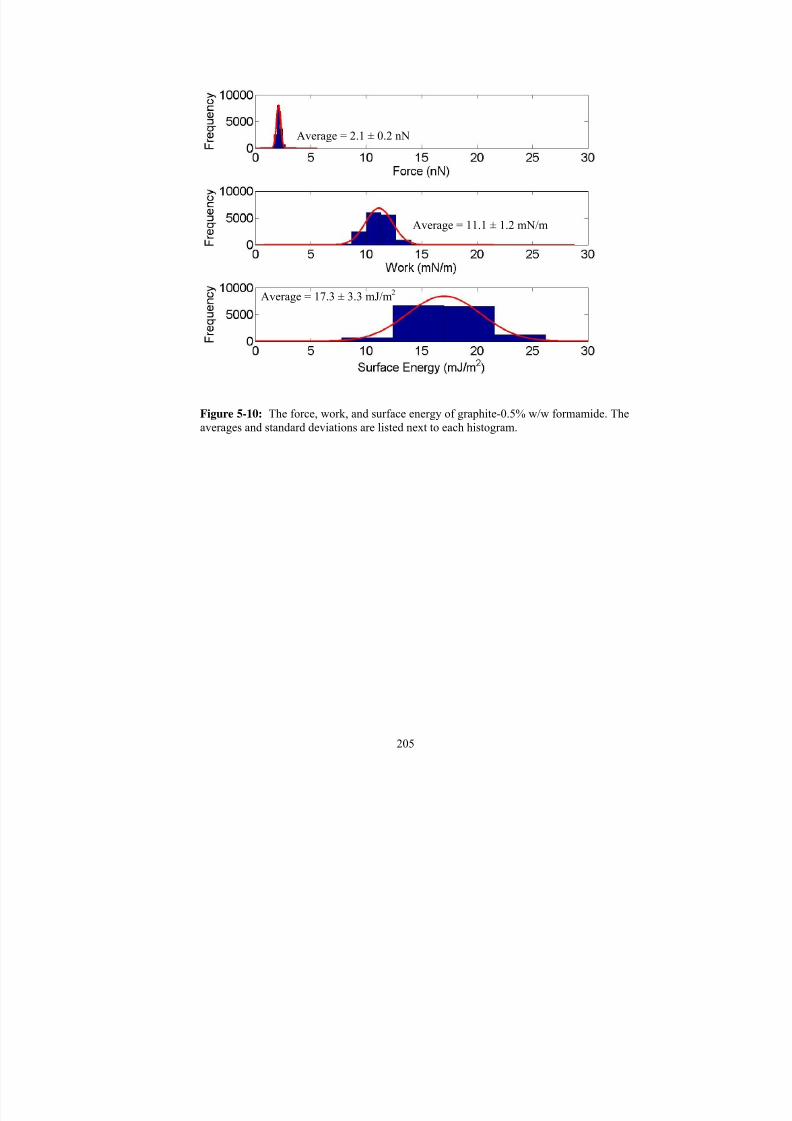
7/27/2019 Atomic Force Microscopy Method Development for Surface Energy Analysis
http://slidepdf.com/reader/full/atomic-force-microscopy-method-development-for-surface-energy-analysis 227/365
205
Figure 5-10: The force, work, and surface energy of graphite-0.5% w/w formamide. Theaverages and standard deviations are listed next to each histogram.
Average = 2.1 ± 0.2 nN
Average = 11.1 ± 1.2 mN/m
Average = 17.3 ± 3.3 mJ/m2

7/27/2019 Atomic Force Microscopy Method Development for Surface Energy Analysis
http://slidepdf.com/reader/full/atomic-force-microscopy-method-development-for-surface-energy-analysis 228/365
206
Figure 5-11: The force, work, and surface energy of graphite-1% w/w formamide. Theaverages and standard deviations are listed next to each histogram.
Average = 2.7 ± 0.4 nN
Average = 14.2 ± 2.1 mN/m
Average = 23.7 ± 6.6 mJ/m2
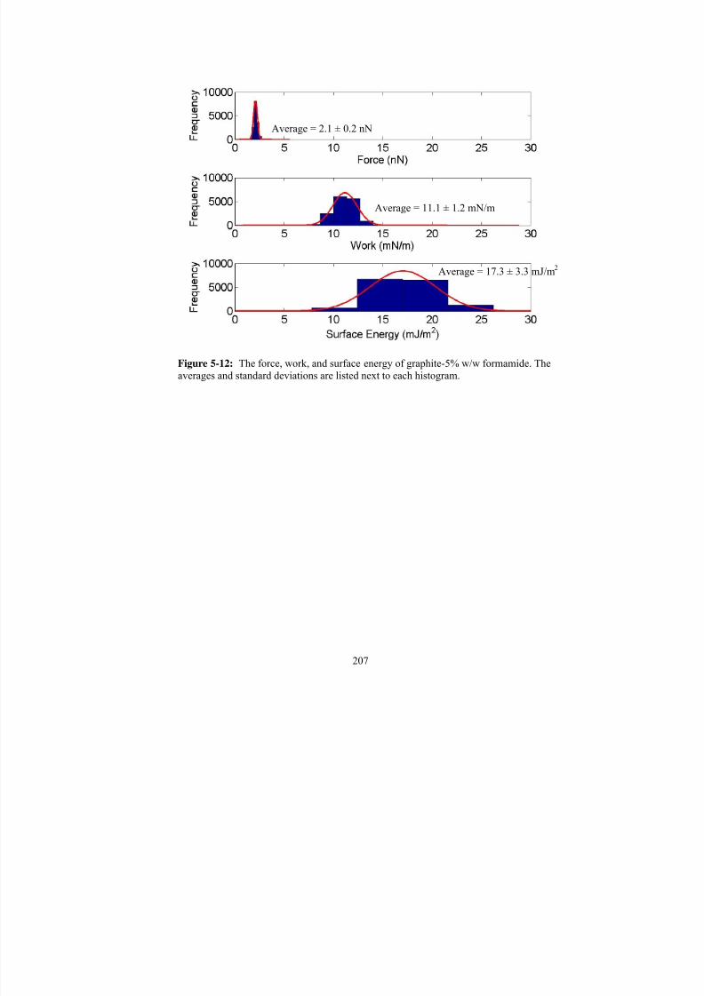
7/27/2019 Atomic Force Microscopy Method Development for Surface Energy Analysis
http://slidepdf.com/reader/full/atomic-force-microscopy-method-development-for-surface-energy-analysis 229/365
207
Figure 5-12: The force, work, and surface energy of graphite-5% w/w formamide. Theaverages and standard deviations are listed next to each histogram.
Average = 2.1 ± 0.2 nN
Average = 11.1 ± 1.2 mN/m
Average = 17.3 ± 3.3 mJ/m2

7/27/2019 Atomic Force Microscopy Method Development for Surface Energy Analysis
http://slidepdf.com/reader/full/atomic-force-microscopy-method-development-for-surface-energy-analysis 230/365
208
Table 5-24: Average solid-liquid surface energy of graphite with dry formamidedetermined using the AFM and contact angle methods.
(Note: Models 2 and 3 do not rely on γsv input to calculate γsl. Therefore the data wasinput into the ambient column for simplicity.)
Ambient
Force
Measurements
Controlled RH
Force
MeasurementsMethod Model
Surface Energy (mJ/m2)
Van Oss et al 10.9 (1.0) 15.2 (1.0)
OWRK 8.5 (1.0) 12.8 (1.0)Model 1
Neumann 5.0 (1.0) 9.3 (1.0)
Model 2 12.5 (2.9) -
Model 3 13.0 (3.3) -
Model 2 γsv 6.7 (1.0) 7.3 (1.0)
AFM
Model 4Model 3 γsv 7.6 (1.0) 7.7 (1.0)
Van Oss et al 13.7 (2.8) NA
OWRK 12.6 (2.2) NAContact
Angle
Neumann 8.7 (1.9) NA

7/27/2019 Atomic Force Microscopy Method Development for Surface Energy Analysis
http://slidepdf.com/reader/full/atomic-force-microscopy-method-development-for-surface-energy-analysis 231/365
209
Table 5-25: Average solid-liquid surface energy of graphite with 0.5% w/wwater/formamide determined using the AFM and contact angle methods.
(Note: Models 2 and 3 do not rely on γsv input to calculate γsl. Therefore the data wasinput into the ambient column for simplicity.)
Ambient
Force
Measurements
Controlled RH
Force
MeasurementsMethod Model
Surface Energy (mJ/m2)
Van Oss et al 13.5 (1.4) 17.8 (1.4)
OWRK 11.1 (1.4) 15.4 (1.4)Model 1
Neumann 7.6 (1.4) 11.9 (1.4)
Model 2 17.3 (3.3) -
Model 3 19.8 (4.9) -
Model 2 γsv 9.3 (1.4) 10.0 (1.4)
AFM
Model 4Model 3 γsv 10.3 (1.4) 10.4 (1.4)
Van Oss et al 18.2 NA
OWRK 14.8 NAContact
Angle
Neumann 11.7 NA

7/27/2019 Atomic Force Microscopy Method Development for Surface Energy Analysis
http://slidepdf.com/reader/full/atomic-force-microscopy-method-development-for-surface-energy-analysis 232/365
210
Table 5-26: Average solid-liquid surface energy of graphite with 1% w/wwater/formamide determined using the AFM and contact angle methods.
(Note: Models 2 and 3 do not rely on γsv input to calculate γsl. Therefore the data wasinput into the ambient column for simplicity.)
Ambient
Force
Measurements
Controlled RH
Force
MeasurementsMethod Model
Surface Energy (mJ/m2)
Van Oss et al 16.0 (2.0) 20.3 (2.0)
OWRK 13.6 (2.0) 17.9 (2.0)Model 1
Neumann 10.1 (2.0) 14.4 (2.0)
Model 2 23.7 (6.6) -
Model 3 25.1 (8.0) -
Model 2 γsv 11.8 (2.0) 12.5 (2.0)
AFM
Model 4Model 3 γsv 12.8 (2.0) 12.9 (2.0)
Van Oss et al 13.6 NA
OWRK 12.9 NAContact
Angle
Neumann 8.8 NA

7/27/2019 Atomic Force Microscopy Method Development for Surface Energy Analysis
http://slidepdf.com/reader/full/atomic-force-microscopy-method-development-for-surface-energy-analysis 233/365
211
Table 5-27: Average solid-liquid surface energy of graphite with 5% w/wwater/formamide determined using the AFM and contact angle methods.
(Note: Models 2 and 3 do not rely on γsv input to calculate γsl. Therefore the data wasinput into the ambient column for simplicity.)
Ambient
Force
Measurements
Controlled RH
Force
MeasurementsMethod Model
Surface Energy (mJ/m2)
Van Oss et al 17.6 (1.9) 21.9 (1.9)
OWRK 15.2 (1.9) 19.5 (1.9)Model 1
Neumann 11.7 (1.9) 16.0 (1.9)
Model 2 -
Model 3 31.4 (8.5) -
Model 2 γsv 13.4 (1.9) 14.1 (1.9)
AFM
Model 4Model 3 γsv 14.4 (1.9) 14.5 (1.9)
Van Oss et al 16.3 NA
OWRK 14.0 NAContact
Angle
Neumann 10.6 NA

7/27/2019 Atomic Force Microscopy Method Development for Surface Energy Analysis
http://slidepdf.com/reader/full/atomic-force-microscopy-method-development-for-surface-energy-analysis 234/365
212
5.1.2.4 Ethylene Glycol Solid-Liquid Surface Energy
The spring constant, tip radii, and tip-liquidethylene glycol surface energies were measured to
determine the solid-liquid surface energy of mica in ethylene glycol. Table 5-28 shows
the values used to calculate mica solid-liquidethylene glycol surface energy.
Ethylene glycol was dried using molecular sieves, then rehydrated to 0.5%, 1%, and 5%
w/w water/ethylene glycol prior to use in AFM and contact angle measurements. Water
content was measured using Coulometric Karl Fisher titration. Each liquid was used the
day it was prepared.
Force measurements were made on mica in ethylene glycol using the tips in Table 5-28.
The data analysis was performed in SAS and JMP. The statistics for mica-dried, -0.5%,
-1%, and -5% w/w water/ethylene glycol are listed in Table 5-29, Table 5-30, Table
5-31, and Table 5-32. The p values were all greater than 0.05, meaning the null
hypotheses was accepted. The average values and data for the force, work, and surface
energy of graphite with dry formamide, 0.5%, 1%, and 5% are shown in Figure 5-13,
Figure 5-14, Figure 5-15, and Figure 5-16.

7/27/2019 Atomic Force Microscopy Method Development for Surface Energy Analysis
http://slidepdf.com/reader/full/atomic-force-microscopy-method-development-for-surface-energy-analysis 235/365
213
Table 5-28: Tip radius and average tip-liquid surface energy (standard deviation) arelisted for the AFM tips used to measure the solid-liquid surface energy of mica inethylene glycol. There are four conditions listed for ethylene glycol, dried, 0.5%, 1%,and 5% w/w water in ethylene glycol.
Tip Condition Springconstant
(N/m)
Radius(nm)
Force(nN)
Work (mN/m)
SurfaceEnergy
(mJ/m2)
1 40 0.4 (0.1) 2.1 (0.6) 1.0 (0.3)
2 42 0.4 (0.2) 1.9 (1.0) 1.0 (0.5)
3
Dry
40 0.3 (0.1) 1.8 (0.5) 0.9 (0.3)
1 40 0.4 (0.1) 2.1 (0.5) 1.0 (0.2)
2 42 0.4 (0.2) 2.2 (1.0) 1.1 (0.5)
3
0.5% w/w water
40 0.8 (0.2) 3.9 (0.8) 1.9 (0.4)
1 40 0.5 (0.1) 2.4 (0.3) 1.2 (0.1)
2 42 0.5 (0.1) 2.4 (0.6) 1.2 (0.3)
3
1% w/w water
40 0.5 (0.1) 2.7 (0.4) 1.3 (0.2)
1 40 0.5 (0.1) 2.4 (0.3) 1.2 (0.1)
2 42 0.5 (0.1) 2.4 (0.6) 1.2 (0.3)
3
5% w/w water
.04
40 0.5 (0.1) 2.7 (0.3) 1.3 (0.1)

7/27/2019 Atomic Force Microscopy Method Development for Surface Energy Analysis
http://slidepdf.com/reader/full/atomic-force-microscopy-method-development-for-surface-energy-analysis 236/365
214
The average force of adhesion did not vary on mica with the rehydrated ethylene glycol.
This meant that the calculated solid-liquid surface energy should remain constant barring
any variations in the tip-liquid. Table 5-28 indicates there are no changes in the tip-
liquid surface energy. Thus, the water in the ethylene glycol had no effect on the AFM
measurements on mica. However, the contact angle measurements with rehydrated
ethylene glycol did show a difference. The measured contact angle with dried ethylene
glycol was 23.1 ± 1.2. The angle increased with the addition of 0.5% w/w water from
23.1 to 30.9 ± 1.3. It increased again 2 more degrees with 1% w/w water, and then fell
back down to 30.5 ± 1.3 with 5% w/w water (Table 2-9). The increase in the angles alsoincreased the contact angle solid-liquid surface energy of mica-ethylene glycol.
However, the same trend was not observed with the AFM. The increase in the contact
angle measurements due to the addition of water was unexpected. Since water has a
strong interaction with mica, it was thought that the presence of water would reduce the
contact angle measurements. This verified Good and Zografi’s conclusion that solutions
cannot be used to measure contact angles.[17, 22] As for the AFM, the forces stayed
relatively constant and subsequently so did the solid-liquid surface energies. There were
changes observed in the surface energy measurements between graphite and hydrated
formamide. However, the AFM did not detect a change in the interaction when ethylene
glycol was hydrated. A decrease in surface energy was predicted in the presence of more
water. However, the miscibility of the water in ethylene glycol was high and allowed for
all water molecules present to interact with the surface of mica. Therefore, the
prediction was incorrect.

7/27/2019 Atomic Force Microscopy Method Development for Surface Energy Analysis
http://slidepdf.com/reader/full/atomic-force-microscopy-method-development-for-surface-energy-analysis 237/365
215
The force of adhesion measurements were expected to fall somewhere between the force
measurements from diiodomethane and water because ethylene glycol has similar polar
and nonpolar components. Therefore, the surface energy was also projected to be in the
middle. Once again, the results from mica contact angle measurements and AFM
measurements were difficult to compare because of contact angle model limitations.
With mica, it was determined that model 1 does not work. The variability in the contact
angle measurements was too great to have any use with AFM measurements. Model 2
and 3 give results that could be plausible considering that scientifically, the surface
energy trend should be:
γsldiiodomethane > γsletheylene glycol > γslwater
where solid-liquid surface energy of diiodomethane is the largest and solid-liquid surface
energy of water is the smallest. Overall, model 4 upholds this trend as well. The only
difference in models 2, 3, and 4 was the distribution of the solid-liquid surface energies.
For model 2 and 3 the range of the three solid-liquids surface energy was from 1 to 14
mJ/m2, where the range in model 4 was from 3 to 9 mJ/m2. Unfortunately, it is still not
apparent which model is best for polar surfaces. The geometric mean was developed for
van der Waals forces, and model 4 assumes the surface molecules will not rearrange from
a vapor environment to a liquid environment. While this assumption may hold on inert
surfaces, it will be challenged in chapter 6 with a crystalline compound.
The statistics from the ethylene glycol studies did not require rejection of the null
hypothesis under any solvent variation. The variability between the mica samples and the
mica-ethylene glycol interaction did not increase significantly with the increase in water.
Most of the variability was attributed to the overall residual error of the measurements.

7/27/2019 Atomic Force Microscopy Method Development for Surface Energy Analysis
http://slidepdf.com/reader/full/atomic-force-microscopy-method-development-for-surface-energy-analysis 238/365
216
These studies differed from graphite in regards to the fact that the water interaction was
strong with mica. The AFM did not detect differences in the solutions as it did with
graphite and rehydrated formamide. Therefore, it could be similar to the phenomenon
discussed with contact angle measurements. The adsorption of the water might not be
homogeneous and therefore, the changes in the liquids’ properties might not be reflected
in contact angle measurements or AFM measurements. Therefore, in addition to the
formamide results, these results justify the use of pure solvents with the AFM and contact
angle methods.

7/27/2019 Atomic Force Microscopy Method Development for Surface Energy Analysis
http://slidepdf.com/reader/full/atomic-force-microscopy-method-development-for-surface-energy-analysis 239/365
217
Table 5-29: Mixed model statistics for mica AFM measurements with dry ethyleneglycol. a) Repeated measures ANOVA for within subject effects, b) repeated measuresANOVA for between subjects, and c) the variable that demonstrates the largest percentage of variance for mica – dry ethylene glycol AFM measurements.
Degrees of
Freedom
Sum of
Square
Mean
Square F Value pLocation 9 10.8 1.2 2.06 0.09Location*Mica 9 6.9 0.8 1.32 0.29Location*Tip 18 18.9 1.1 1.81 0.11Error 18 10.4 0.6 - -
Degrees of Freedom
Sum of Square
MeanSquare
F Value p
Mica 1 0.2 0.2 0.56 0.53Tip 2 0.8 0.4 1.07 0.48Error 2 0.7 0.4 - -
Variable % of the Total % TruncatedMica -0.7 0.0Tip 0.2 0.2Mica*Tip 10.2 8.7Mica*Tip*Location (Error) 106.3 91.1
Total 100.0 100.0
a)
b)
c)

7/27/2019 Atomic Force Microscopy Method Development for Surface Energy Analysis
http://slidepdf.com/reader/full/atomic-force-microscopy-method-development-for-surface-energy-analysis 240/365
218
Table 5-30: Mixed model statistics for mica AFM measurements with 0.5% w/wethylene glycol. a) Repeated measures ANOVA for within subject effects, b) repeatedmeasures ANOVA for between subjects, and c) the variable that demonstrates the largest percentage of variance for mica – 0.5% w/w ethylene glycol AFM measurements.
Degrees of
Freedom
Sum of
Square
Mean
Square F Value pLocation 9 6.6 0.7 0.70 0.70Location*Mica 9 8.3 0.9 0.8 0.56Location*Tip 18 5.7 0.3 0.3 0.99Error 18 18.9 1.1 - -
Degrees of Freedom
Sum of Square
MeanSquare
F Value p
Mica 1 4.6 4.6 3.88 0.19Tip 2 4.6 2.3 1.95 0.34Error 2 2.36 1.18 - -
Variable % of the Total % TruncatedMica 12.0 12.0Tip 5.9 5.9Mica*Tip 4.8 4.8Mica*Tip*Location (Error) 77.2 77.2
Total 100.0 100.0
a)
b)
c)
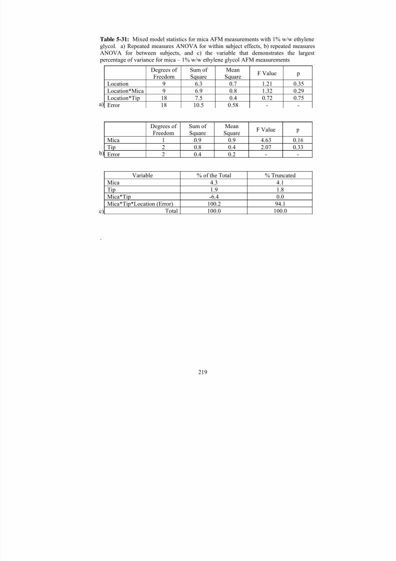
7/27/2019 Atomic Force Microscopy Method Development for Surface Energy Analysis
http://slidepdf.com/reader/full/atomic-force-microscopy-method-development-for-surface-energy-analysis 241/365
219
Table 5-31: Mixed model statistics for mica AFM measurements with 1% w/w ethyleneglycol. a) Repeated measures ANOVA for within subject effects, b) repeated measuresANOVA for between subjects, and c) the variable that demonstrates the largest percentage of variance for mica – 1% w/w ethylene glycol AFM measurements
Degrees of
Freedom
Sum of
Square
Mean
Square F Value pLocation 9 6.3 0.7 1.21 0.35Location*Mica 9 6.9 0.8 1.32 0.29Location*Tip 18 7.5 0.4 0.72 0.75Error 18 10.5 0.58 - -
Degrees of Freedom
Sum of Square
MeanSquare
F Value p
Mica 1 0.9 0.9 4.63 0.16Tip 2 0.8 0.4 2.07 0.33Error 2 0.4 0.2 - -
Variable % of the Total % TruncatedMica 4.3 4.1Tip 1.9 1.8Mica*Tip -6.4 0.0Mica*Tip*Location (Error) 100.2 94.1
Total 100.0 100.0
.
a)
b)
c)

7/27/2019 Atomic Force Microscopy Method Development for Surface Energy Analysis
http://slidepdf.com/reader/full/atomic-force-microscopy-method-development-for-surface-energy-analysis 242/365
220
Table 5-32: Mixed model statistics for mica AFM measurements with 5% w/w ethyleneglycol. a) Repeated measures ANOVA for within subject effects, b) repeated measuresANOVA for between subjects, and c) the variable that demonstrates the largest percentage of variance for mica – 5% w/w ethylene glycol AFM measurements.
Degrees of
Freedom
Sum of
Square
Mean
Square F Value pLocation 9 9.5 1.1 0.53 0.84Location*Mica 9 9.3 1.0 0.52 0.84Location*Tip 18 21.5 1.2 0.60 0.86Error 18 36.1 2.0 - -
Degrees of Freedom
Sum of Square
MeanSquare
F Value p
Mica 1 0.02 0.02 0.04 0.86Tip 2 16.8 8.4 14.65 0.06Error 2 1.1 0.6 - -
Variable % of the Total % TruncatedMica -1.0 0.0Tip 22.1 20.8Mica*Tip -5.2 0.0Mica*Tip*Location (Error) 84.1 79.2
Total 100.0 100.0
a)
b)
c)

7/27/2019 Atomic Force Microscopy Method Development for Surface Energy Analysis
http://slidepdf.com/reader/full/atomic-force-microscopy-method-development-for-surface-energy-analysis 243/365
221
Figure 5-13: The force, work, and surface energy of mica-dried ethylene glycol. Theaverages and standard deviations are listed next to each histogram.
Average = 0.9 ± 0.2 nN
Average = 4.7 ± 0.9 mN/m
Average = 5.7 ± 2.0 mJ/m2
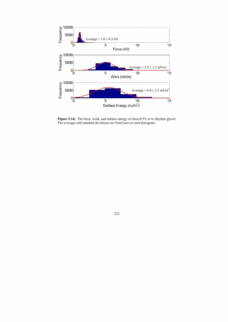
7/27/2019 Atomic Force Microscopy Method Development for Surface Energy Analysis
http://slidepdf.com/reader/full/atomic-force-microscopy-method-development-for-surface-energy-analysis 244/365
222
Figure 5-14: The force, work, and surface energy of mica-0.5% w/w ethylene glycol.The averages and standard deviations are listed next to each histogram.
Average = 1.0 ± 0.3 nN
Average = 5.5 ± 1.5 mN/m
Average = 6.0 ± 2.2 mJ/m2
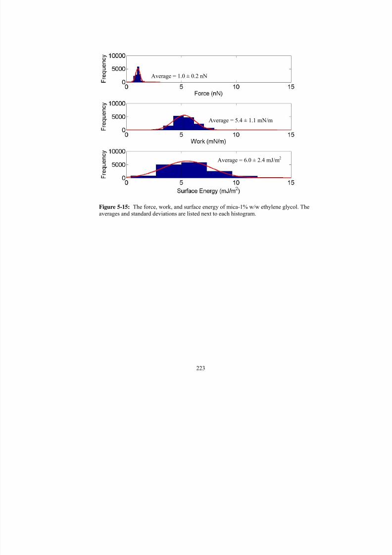
7/27/2019 Atomic Force Microscopy Method Development for Surface Energy Analysis
http://slidepdf.com/reader/full/atomic-force-microscopy-method-development-for-surface-energy-analysis 245/365
223
Figure 5-15: The force, work, and surface energy of mica-1% w/w ethylene glycol. Theaverages and standard deviations are listed next to each histogram.
Average = 1.0 ± 0.2 nN
Average = 5.4 ± 1.1 mN/m
Average = 6.0 ± 2.4 mJ/m2
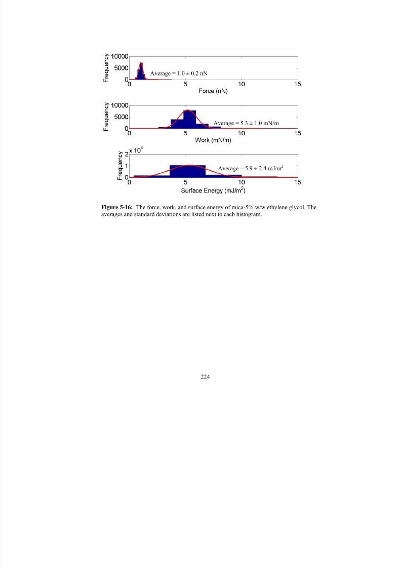
7/27/2019 Atomic Force Microscopy Method Development for Surface Energy Analysis
http://slidepdf.com/reader/full/atomic-force-microscopy-method-development-for-surface-energy-analysis 246/365
224
Figure 5-16: The force, work, and surface energy of mica-5% w/w ethylene glycol. Theaverages and standard deviations are listed next to each histogram.
Average = 1.0 ± 0.2 nN
Average = 5.3 ± 1.0 mN/m
Average = 5.9 ± 2.4 mJ/m2

7/27/2019 Atomic Force Microscopy Method Development for Surface Energy Analysis
http://slidepdf.com/reader/full/atomic-force-microscopy-method-development-for-surface-energy-analysis 247/365
225
Table 5-33: Average solid-liquid surface energy of mica and dry ethylene glycoldetermined using the AFM and contact angle methods.
(Note: Models 2 and 3 do not rely on γsv input to calculate γsl. Therefore the data wasinput into the ambient column for simplicity.)
Ambient
Force
Measurements
Controlled RH
Force
MeasurementsMethod Model
Surface Energy (mJ/m2)
Van Oss et al 0.5 (0.8) 14.0 (0.8)
OWRK 24.4 (0.8) 37.9 (0.8)Model 1
Neumann 16.2 (0.8) 29.7 (0.8)
Model 2 5.7 (2.0) -
Model 3 5.7 (2.1) -
Model 2 γsv 4.2 (0.8) 3.3 (0.8)
AFM
Model 4Model 3 γsv 4.0 (0.8) 3.8 (0.8)
Van Oss et al -3.6 NA
OWRK 21.1 NAContact
Angle
Neumann 13.5 NA

7/27/2019 Atomic Force Microscopy Method Development for Surface Energy Analysis
http://slidepdf.com/reader/full/atomic-force-microscopy-method-development-for-surface-energy-analysis 248/365
226
Table 5-34: Average solid-liquid surface energy of mica with 0.5% w/w water/ethyleneglycol determined using the AFM and contact angle methods.
(Note: Models 2 and 3 do not rely on γsv input to calculate γsl. Therefore the data wasinput into the ambient column for simplicity.)
Ambient
Force
Measurements
Controlled RH
Force
MeasurementsMethod Model
Surface Energy (mJ/m2)
Van Oss et al 1.0 (1.2) 14.5 (1.2)
OWRK 24.9 (1.2) 38.4 (1.2)Model 1
Neumann 16.7 (1.2) 30.2 (1.2)
Model 2 6.0 (2.2) -
Model 3 6.0 (2.3) -
Model 2 γsv 4.7 (1.2) 3.8 (1.2)
AFM
Model 4Model 3 γsv 4.5 (1.2) 4.3 (1.2)
Van Oss et al -0.4 NA
OWRK 22.8 NAContact
Angle
Neumann 15.7 NA

7/27/2019 Atomic Force Microscopy Method Development for Surface Energy Analysis
http://slidepdf.com/reader/full/atomic-force-microscopy-method-development-for-surface-energy-analysis 249/365
227
Table 5-35: Average solid-liquid surface energy of mica with 1% w/w water/ethyleneglycol determined using the AFM and contact angle methods.
(Note: Models 2 and 3 do not rely on γsv input to calculate γsl. Therefore the data wasinput into the ambient column for simplicity.)
Ambient
Force
Measurements
Controlled RH
Force
MeasurementsMethod Model
Surface Energy (mJ/m2)
Van Oss et al 0.9 (1.1) 14.4 (1.1)
OWRK 24.8 (1.1) 38.3 (1.1)Model 1
Neumann 16.6 (1.1) 30.1 (1.1)
Model 2 6.0 (2.4) -
Model 3 6.1 (2.5) -
Model 2 γsv 4.6 (1.1) 3.7 (1.1)
AFM
Model 4Model 3 γsv 4.4 (1.1) 4.2 (1.1)
Van Oss et al 1.2 NA
OWRK 23.7 NAContact
Angle
Neumann 16.2 NA

7/27/2019 Atomic Force Microscopy Method Development for Surface Energy Analysis
http://slidepdf.com/reader/full/atomic-force-microscopy-method-development-for-surface-energy-analysis 250/365
228
Table 5-36: Average solid-liquid surface energy of mica with 5% w/w water/ethyleneglycol determined using the AFM and contact angle methods.
(Note: Models 2 and 3 do not rely on γsv input to calculate γsl. Therefore the data wasinput into the ambient column for simplicity.)
Ambient
Force
Measurements
Controlled RH
Force
MeasurementsMethod Model
Surface Energy (mJ/m2)
Van Oss et al 0.9 (1.0) 14.4 (1.0)
OWRK 24.8 (1.0) 38.3 (1.0)Model 1
Neumann 16.6 (1.0) 30.1 (1.0)
Model 2 5.9 (2.4) -
Model 3 6.0 (2.6) -
Model 2 γsv 4.6 (1.0) 3.7 (1.0)
AFM
Model 4Model 3 γsv 4.4 (1.0) 4.2 (1.0)
Van Oss et al -0.3 NA
OWRK 22.6 NAContact
Angle
Neumann 15.2 NA

7/27/2019 Atomic Force Microscopy Method Development for Surface Energy Analysis
http://slidepdf.com/reader/full/atomic-force-microscopy-method-development-for-surface-energy-analysis 251/365
229
5.2 Summary
The overall goal of this project was AFM method development for the measurement of
surface energy. In Chapter 4, the equations for converting the AFM force of adhesion
measurements to surface energy were introduced. In this chapter the goals were:
1. To measure the forces of adhesion on graphite and mica in vapor and liquid
conditions.
2. To evaluate the statistical model discussed in Chapter 3.
3. To evaluate the four AFM surface energy models developed in Chapter 4.
4. To compare the results obtained from the AFM surface models to contact angle
results.
The collection of data began with the ambient and controlled environmental conditions,
measuring the solid-vapor surface energy of mica and graphite. The controlled
environment was tested because of the capillary effect present in ambient conditions.The capillary effect was shown to increase the measured force of adhesion, and that
relative humidity needed to be regulated to find the “true” surface-energy. This
phenomenon was observed between the mica ambient and controlled RH measurements.
The surface energy significantly decreased when the humidity was lowered. The
difference between the graphite ambient and controlled RH was very small if not absent
entirely. Therefore, it was concluded that non-polar, hydrophobic surfaces have less
interaction with water and subsequently less capillary effects as compared to a polar,
hydrophilic surface like mica. The mica results had a substantial change in solid-vapor
surface energy when the humidity was controlled.

7/27/2019 Atomic Force Microscopy Method Development for Surface Energy Analysis
http://slidepdf.com/reader/full/atomic-force-microscopy-method-development-for-surface-energy-analysis 252/365
230
To evaluate the overall hypothesis and demonstrate the AFM’s capability for determining
surface energy, results were compared to contact angle measurements. For graphite, both
models 2 and 3 were useful for calculating solid-vapor surface energy when compared to
the contact angle surface energy. For ambient mica, surface energy was comparable with
the van Oss contact angle method. Controlled solid-vapor surface energy was not
comparable to any contact angle results. Thus, it was also concluded that the
environmental conditions can affect the solid-vapor surface energy. As a result, it may be
necessary to investigate surface energy in a lower humidity environment. This puts
contact angles at a disadvantage since some liquids require that an environmentalchamber be saturated with the liquid to measure an equilibrium contact angle. However,
the AFM is ideally suited for this type of measurement, and may be better adapted for
surface energy studies.
As for the four AFM surface energy models, there was not a substantial difference
between models 2 and 3. Since there were comparable results between the AFM and
contact angle, the models were effective for the calculation of surface energy even with
the necessary assumptions. It was shown that the universal β from contact angle
measurements was not applicable to the AFM. A smaller β than the universal β was
necessary to return the experimental work values. However, since model 3 did not result
in values different from model 2, the modification was not an improvement from the
geometric mean. Since, the geometric mean was developed for van der Waals forces, it
was not clear if the use of the equation with polar surfaces would overestimate or
underestimate the surface energy. Unfortunately, the mica AFM measurements could not
be compared to the contact angle results because of the limitations observed with the

7/27/2019 Atomic Force Microscopy Method Development for Surface Energy Analysis
http://slidepdf.com/reader/full/atomic-force-microscopy-method-development-for-surface-energy-analysis 253/365
231
indirect models. Only the van Oss model was comparable to the mica-ambient AFM
solid-vapor surface energy.
For solid-liquid surface energy investigation with graphite, AFM results were comparable
to contact angle results illustrating the ability of the AFM to be used for hydrophobic
surfaces. Models 2 and 3 were effective in determining surface energy for all three
conditions: water, formamide, and diiodomethane. However, all four models were useful
when using formamide. Formamide had similar surface tension components as compared
to the extremes of water and diiodomethane surface tension components. The contact
angle method showed limitations at the extremes. The difficulty for contact angle
measurements is mostly from the limited number of equations. Young's equation
balances the forces, often yielding a negative solid-liquid surface. This was observed
with graphite-diiodomethane. These negative numbers make it difficult to determine the
applicability of the AFM. Thus, dried formamide showed the effectiveness of the AFM
surface energy models. However, because of extremes it was easier to decide that model
2 was the most useful surface energy model. Models 1 and 4 break down when applied
to extreme interactions. Models 1 and 4 also break down later in Chapter 6 when
investigating inert surfaces. Model 2 is limited because the geometric mean is based only
on van der Waals interactions. However, this model has been used for other interactions.
In order to use the geometric mean with the polar and AB interactions, the assumption
made is that the pure components’ differences in electronic properties and molecular size
are small. [21] The advantage of using the geometric mean is that the solid-liquid surface
energy is not dependent on the interaction of the surface in vapor. Depending on solid-
vapor surface energy measurements to determine the surface-tip interaction, is similar to

7/27/2019 Atomic Force Microscopy Method Development for Surface Energy Analysis
http://slidepdf.com/reader/full/atomic-force-microscopy-method-development-for-surface-energy-analysis 254/365
232
the dependence contact angle has the measurements of three liquids. It seems the fewer
dependent variables there are, the easier it is to determine surface energy.
The solid-liquid surface energy for mica was difficult to compare directly to results from
the contact angle method because of the equation limitation of the contact angle method.
However, the trend was still there. The contact angle results showed:
θ diiodomethane > θ ethylene glycol > θ water
This same observation was seen with the forces:
F diiodomethane > F ethylene glycol > F water
Therefore, if the solid-liquid surface energy (γsl) for contact angle measurements could be
used, it would follow the same trend that was seen from the AFM measurements:
γsl-diiodomethane > γ sl-ethylene glycol > γ sl-water
Although the final results were difficult to compare, model 1 was ruled out because of the
contact angle variability on hydrophilic surfaces. This variability caused a much larger
range in the solid-liquid surface energy for mica with water, diiodomethane, and ethylene
glycol. Model 2 and 3 showed distinct ranges between the three solvents on mica.
Model 4 was also useful, but had a smaller distribution of surface energy. Also, it was not
clear until Chapter 6 that model 4 would become invalid. However, for inert hydrophilic
surfaces, model 4 could be used. Model 3 did not offer a benefit over model 2. It was
thought the modification would be needed on hydrophilic surface. These results showed
that if the difference between the binary components' electronic properties and molecular
size are small, the geometric mean could be applied to van der Waals interactions and
polar interactions. Yet still, it was the limitations of the contact angle method that made

7/27/2019 Atomic Force Microscopy Method Development for Surface Energy Analysis
http://slidepdf.com/reader/full/atomic-force-microscopy-method-development-for-surface-energy-analysis 255/365
233
it difficult to evaluate the AFM’s capabilities and the functionality of the AFM surface
energy models on a hydrophilic surface.
The hygroscopic liquid measurements also made it clear that care should be taken to dry
solvents prior to use so that the “true” solid-liquid surface energy can be observed. It was
also necessary so AFM results were not confounded by the presence of water. The
results from hydrated ethylene glycol and formamide showed that the increase in water
started to affect the spread and repeatability of the AFM measurements.
Finally, to make a concise recommendation on a surface energy model, investigation on a
surface that has both polar and nonpolar interactions is required. The promising results
from graphite-formamide indicate an intermediate interaction is needed to evaluate the
AFM's capability. This intermediate would circumvent the limitations of the contact
angle and allow for a full comparison with AFM results.
Since this was not included in the scope of this work, all of the models were carried
through to Chapter 6 where the AFM was applied to measurements on crystalline
surfaces. The crystalline system was chosen so that the strengths learned in this chapter
could be leveraged. Since the best results were obtained from graphite, it was decided to
try and identify a crystalline system with more hydrophobicity.
Copyright © Clare Aubrey Medendorp 2011

7/27/2019 Atomic Force Microscopy Method Development for Surface Energy Analysis
http://slidepdf.com/reader/full/atomic-force-microscopy-method-development-for-surface-energy-analysis 256/365
234
Chapter 6 – Applying the AFM Methodology to Aspirin
The goal of this chapter is to apply the methodology in Chapter 3, the surface energy
models in Chapter 4 and the knowledge obtained in Chapter 5 to determine the solid-
vapor and solid-liquid surface energy of a crystalline material. In order to explain the
surface energy results, there has to be a fundamental understanding of the surface
chemistry. Therefore a review of the structure and chemical moieties of the model
crystalline material is also given.
6.1 Aspirin Crystal Growth and Indexing Review
6.1.1 Introduction
The majority of pharmaceutical materials are in the solid crystalline form. This includes
the active pharmaceutical ingredient and excipients used in formulating the solid dosage
form. The arrangement or packing of the molecules in a crystal determines it physical,
chemical, and mechanical properties. These properties also vary when crystal packing is
fixed and the shape or crystal habit is modified. Thus control of crystal packing and habit
is crucial in the pharmaceutical industry.[63] Ritonavir is a well known example of the
importance of controlling crystal packing. This product was pulled from the market after
multiple batches failed dissolution testing. X-Ray crystallography studies were
performed on the failed batches and a new polymorph was discovered that was more
thermodynamically stable than the marketed form.[64] Conversely, acetaminophen has
two different polymorphs with Form I being the most thermodynamically stable and is
thus the marketed form. However, the orthorhombic Form II has better compression

7/27/2019 Atomic Force Microscopy Method Development for Surface Energy Analysis
http://slidepdf.com/reader/full/atomic-force-microscopy-method-development-for-surface-energy-analysis 257/365
235
behavior for tableting. So to improve tableting of Form I, studies have been done to
modify the crystal habit.[65]
Crystal habit is governed by the relative rates of particle deposition on the various faces,
with the general rule being, faces that grow the slowest will develop as major faces.
These rates are primarily determined from the binding strength of the solute molecules at
the various crystal surfaces.[66, 67] However, several factors can cause modifications in
the rate of deposition at specific surfaces, thus varying the crystal’s habit. Such factors
include temperature, degree of supersaturation, solvents, and additives/impurities.[63]
The ability of solvents to enhance or inhibit crystal growth is not completely resolved,
but has been approached with two different theories. The first theory states that favorable
interactions between solute and solvent on specific faces leads to reduced interfacial
tension, causing a transition from a smooth to a rough interface and a concomitant faster
surface growth.[68] The second theory proposed states that it is preferential adsorption at
specific faces that will inhibit crystal faces growth. The removal of bound solvent
adsorbed poses an additional energy barrier for continued growth, thus slowing down the
growth on the crystal face.[69]
Studies have also been done on the influence of “tailor-made” additives on crystal habit.
It is believed these so called “tailor-made” additives inhibit growth through preferential
adsorption at specific faces. These “tailor-made” additives have a similar base molecule
with one altered functional moiety. Lahav and coworkers have proposed that structurally
similar additives will adsorb stereospecifically because of the similar shape with the host
molecule. The adsorbed additive essentially replaces the host molecules and hinders or
slows adsorption of more solute molecules to this face. This growth change occurs

7/27/2019 Atomic Force Microscopy Method Development for Surface Energy Analysis
http://slidepdf.com/reader/full/atomic-force-microscopy-method-development-for-surface-energy-analysis 258/365
236
because the additive molecule emerges from the crystal surface in a different orientation
than the host molecule, disrupting the previous repeating pattern.[67, 69, 70]
6.1.2 Background on aspirin
The model crystalline compound chosen was acetylsalicylic acid (ASA). ASA is still
used today as an analgesic and antiplatelet medication. For many years it was thought
that there were at least two polymorphs of ASA.[71] There has been a very recent
discovery that eluded to a second form,[72] but the stability and elucidation of this
polymorph has been questioned.[73] Before this second polymorph was found only
different crystal habits had been observed.[71]
Depending on the conditions of preparation, pharmaceutical crystals may exhibit
variations in habit with the consequence that interfacial properties can be modulated by
the various morphologically important faces. This is what made aspirin an interesting
molecule to study, because of the reported literature differences in morphology.[71] To
study crystal habit and understand the physical and chemical properties it is crucial to
have molecular level knowledge of the crystal structure at the surface.[74] In order to
determine and characterize the surface structure of particular crystal faces, the molecular
packing and the face indices must be assigned properly.
Despite the persistent investigations since its discovery in late 1800s,[75] it was
discovered early in the aspirin studies that there is still confusion over classification of
the crystal morphology. In the 1930s, the lattice parameters of aspirins were defined by
X-ray diffraction (XRD) using oscillation and Weissenberg photographs. The conclusion
was aspirin belonged to the P21/a (a nonstandard setting of space group number 14)
space group.[76, 77] If this space group is used, the predominant face is identified as

7/27/2019 Atomic Force Microscopy Method Development for Surface Energy Analysis
http://slidepdf.com/reader/full/atomic-force-microscopy-method-development-for-surface-energy-analysis 259/365
237
(001).[78, 79] However, the first full structure determination by single crystal XRD in
1964,[80] assigned a different setting of the same space group, that is, P21/c.[81-83] In
this setting, the largest face is (100).[84, 85] A likely cause of the confusion over face
indexing was then the use of alternative space group settings, which was exacerbated by
the almost identical metrics of the a and c axes.[86] Consequently the two possible space
groups caused the functional groups to be assigned improperly to the indexed face. If
P21/a is used for indexing instead of P21/c, any conclusions drawn with regard to surface
properties of a particular face will be in error, particularly from the viewpoint of
structure-property relationships.[86] Several studies, included contact angle work fromthe Li lab, have probed the chemical nature of functional groups exposed on the two
major faces of aspirin crystals an incorrectly concluded that the (100) face was more
hydrophilic than the (001) face due to the presence of the carboxyl group on the
(100).[87] The conclusion that the smaller contact angle observed with water was on the
supposed (100) face, was justified by the presence of the carboxyl group. Upon closer
inspection of the face indexing of aspirin single crystals with XRD, it was shown that the
common assignment of the (100) face as more hydrophilic (due to the exposure of
carboxyl group) is not correct.[86] The confusion seemed to stem from the original
assignment of the space group and indices of the crystal faces.[77-79, 88] Therefore
before the surface energy can be evaluated with contact angle and AFM measurements,
the crystal indexing must be clear. This lab published a communication that presented
experimental evidence to clarify the difference between the two major faces of aspirin
crystal. This published communication included contact angle data for further
interpretation of surface wettability.[86] However, in this chapter we will further the

7/27/2019 Atomic Force Microscopy Method Development for Surface Energy Analysis
http://slidepdf.com/reader/full/atomic-force-microscopy-method-development-for-surface-energy-analysis 260/365
238
contact angle data and add the AFM data to present solid-vapor and solid-liquid surface
energy. These results will be added to the initial investigation from the communication.
This will also allow for testing the four AFM surface energy models and the method
developed in the previous chapters on pharmaceutical crystalline material.
6.1.3 Crystal growth
Aspirin single crystals were grown by slow evaporation from ethanol and acetone.
Aspirin and the solvent were dissolved in a beaker to its solubility (0.2 gm/mL in ethanol
and 0.18 gm/mL in acetone), by stirring. The beakers were covered with Parafilm®.
Small holes were punched through the seal using a needle, and stored in ambient
conditions. Aspirin crystals were grown in water with a supersaturation ratio of 225%
based on its water solubility of 3.3 mg/mL. The beakers were sealed with Parafilm® and
stored in ambient conditions. The morphology of aspirin was also manually generated by
the Cerius2 program (Accelrys, Inc., San Diego, CA) using the single crystal X-ray data
and the observed habits of the crystals grown from the different solvents.[86]
Aspirin crystallized in ethanol, water, and acetone results in plate morphology with two
major faces and a few different minor faces, shown in Figure 6-1. The effects of solvent
on crystallization of aspirin demonstrate some morphological differences but no
polymorphism. This was validated in both the XRD and PXRD studies.[86]
6.1.4 Aspirin crystal structure
The aspirin crystals grown in the Li lab were evaluated by single X-ray diffraction. The
results indicated the crystals were of the monoclinic space group P21/c with a =
11.242(7), b = 6.539(4), c = 11.245(9) Å, and β = 95.9(3)°. These values were in

7/27/2019 Atomic Force Microscopy Method Development for Surface Energy Analysis
http://slidepdf.com/reader/full/atomic-force-microscopy-method-development-for-surface-energy-analysis 261/365
239
agreement with the literature.[80-83] The some controversy exists the elusive second
form (form II) of aspirin has been identified and characterized by single crystal X-ray
diffraction.[72, 73] The unit cell parameters are superficially quite different from those
of form I, although they are likely related. Nonetheless, both forms exhibit the same
space group, P21/c.[89] In our crystallization studies only form I was produced,[86]
though the presence of a very small amount of form II cannot be discounted.[72, 73]
Our results demonstrate that for crystals indexed as P21/c, the largest growth face is
(100) and the second largest is (001), as shown in Figure 6-2. Based on these
assignments and an intimate view of the crystal packing, it is apparent that there are two
possible truncations for the (100) face. One truncation goes through the carboxyl group
and another passes through the acetyloxy groups. It is important to make this distinction
on the (100) face, especially when probing surface properties in relation to functional
groups on that surface. As shown in Figure 6-2, if a surface property, such as wettability,
is measured on the (100) face but explained using the functional groups present on the
(001) face, conclusions will be misleading.[86]
The crucial point is to recognize which functional groups are exposed on the major faces
whether the space group is assigned as P21/a or P21/c. The axes could be assigned
according to any number of conventions, but the functional groups assigned to the
physical faces are invariant. The dominant face will always have the acetyloxy group
(not the carboxyl group as discussed below) and the other major face will always have
the methyl and phenyl groups. This is illustrated in Figure 6-2.[86]

7/27/2019 Atomic Force Microscopy Method Development for Surface Energy Analysis
http://slidepdf.com/reader/full/atomic-force-microscopy-method-development-for-surface-energy-analysis 262/365
240
Figure 6-1: Aspirin crystals grown from a) ethanol, b) acetone, and c) water. Scale barsdenote 1 mm.
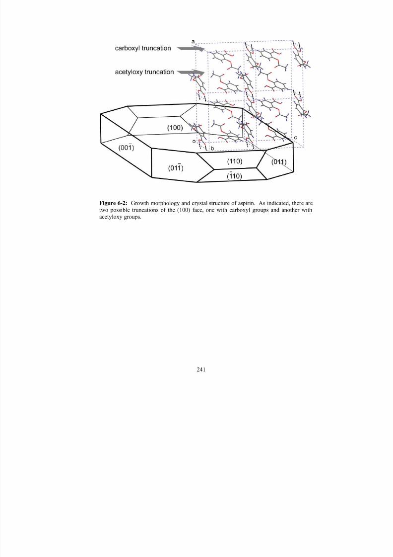
7/27/2019 Atomic Force Microscopy Method Development for Surface Energy Analysis
http://slidepdf.com/reader/full/atomic-force-microscopy-method-development-for-surface-energy-analysis 263/365
241
Figure 6-2: Growth morphology and crystal structure of aspirin. As indicated, there aretwo possible truncations of the (100) face, one with carboxyl groups and another withacetyloxy groups.

7/27/2019 Atomic Force Microscopy Method Development for Surface Energy Analysis
http://slidepdf.com/reader/full/atomic-force-microscopy-method-development-for-surface-energy-analysis 264/365
242
6.2 Contact Angle Method
6.2.1 Contact angles
Contact angles were measured with various solvents on the two major faces of aspirin,
and the results are summarized in Table 6-1. All of the contact angles measured on the
(100) face are larger than those on the (001) face. Due to the polar nature of the solvents
used, the measurements indicate the (100) face is less hydrophilic than the (001),
emphasizing the importance of knowing the surface crystal structure. Although the (100)
face may expose the carboxyl acid group, the contact angle measurements indicate
otherwise. It appears to be the acetyloxy truncation that is exposed, which leads to the
(100) face being less hydrophilic than the (001) face. The hydrogen bonding between
carboxyl groups in the crystal is strong; cleavage through this bonding to expose the
carboxyl group is unlikely. Once again, the relationship between the interfacial
properties and surface structure could be misconstrued when using the improper labeling
and thereby identifying the wrong surface functional groups. If the more hydrophilic face
is mistaken as the (100), carboxyl groups would be thought as the dominant surface
group and that it would be involved in solvent interactions. These results show that the
carboxyl group is not exposed and therefore a lower contact angle by a polar liquid is not
expected.[86]

7/27/2019 Atomic Force Microscopy Method Development for Surface Energy Analysis
http://slidepdf.com/reader/full/atomic-force-microscopy-method-development-for-surface-energy-analysis 265/365
243
Table 6-1: Contact angles on the (100) and (001) faces of aspirin measure in selectedsolvents.
Water Diiodomethane Glycerol
(100) 66.9 ± 2.9 41.2 ± 1.7 65.1 ± 1.1
(001) 56.4 ± 2.4 36.2 ± 1.9 56.5 ± 0.9

7/27/2019 Atomic Force Microscopy Method Development for Surface Energy Analysis
http://slidepdf.com/reader/full/atomic-force-microscopy-method-development-for-surface-energy-analysis 266/365
244
6.2.2 Surface energy calculations from contact angle indirect models
6.2.2.1 Solid-Vapor Surface Energy
Once the contact angles were measured, the three indirect contact angle models discussed
in Chapter 2 were used to calculate solid-vapor surface energy. From the contact angle
data, the (100) and (001) faces of aspirin were more similar to graphite. These faces
showed more of a hydrophobic nature. Therefore, it was hypothesized that the solid-
vapor surface energy calculated using the three models would be more similar than the
results on a hydrophilic surface. The solid vapor surface energies from contact angle data
are shown in Table 6-2. The overall solid-vapor surface energy between each model was
fairly similar, ranging from 40.2 to 42.8 mJ/m2 on the (100) face and 44.6 to 49.2 mJ/m2
on the (001) face. Therefore, as hypothesized, there was not a huge disparity in the
models. While there was roughly a 10 degree difference in water and glycerol contact
angles, the solid-vapor surface energies did not show large differences in the two faces.
Since these two faces are the major faces of aspirin, this was expected given that the
morphology of a crystal is the result of relative growth rates of its various faces, and that
the slowest growing faces are expressed in the crystal habit. The growth rates of the
crystalline faces are determined by intermolecular interaction between the molecules in
the crystal as well as external parameters such as solvent, supersaturation, temperature,
and impurities.[90] As these two faces are major faces, it was expected that their surface
energies would be similar, while minor faces would have distinctly different surface
energies. The minor faces are the faces growing faster and thus "disappearing" or
becoming much smaller in the resultant crystal morphology.
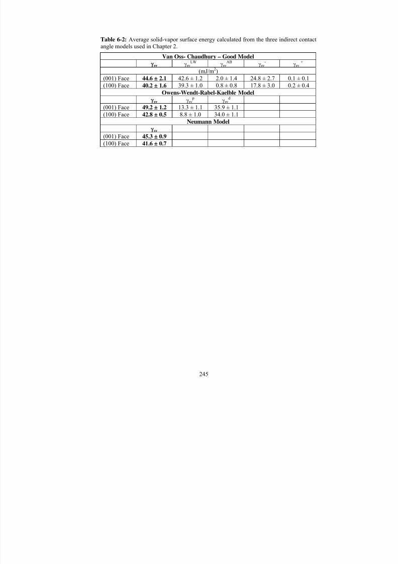
7/27/2019 Atomic Force Microscopy Method Development for Surface Energy Analysis
http://slidepdf.com/reader/full/atomic-force-microscopy-method-development-for-surface-energy-analysis 267/365
245
Table 6-2: Average solid-vapor surface energy calculated from the three indirect contactangle models used in Chapter 2.
Van Oss- Chaudhury – Good Model
γsv γsvLW γsv
AB γsv- γsv
+ (mJ/m2)
(001) Face 44.6 ± 2.1 42.6 ± 1.2 2.0 ± 1.4 24.8 ± 2.7 0.1 ± 0.1(100) Face 40.2 ± 1.6 39.3 ± 1.0 0.8 ± 0.8 17.8 ± 3.0 0.2 ± 0.4
Owens-Wendt-Rabel-Kaelble Model
γsv γsv p γsv
d
(001) Face 49.2 ± 1.2 13.3 ± 1.1 35.9 ± 1.1(100) Face 42.8 ± 0.5 8.8 ± 1.0 34.0 ± 1.1
Neumann Model
γsv
(001) Face 45.3 ± 0.9
(100) Face 41.6 ± 0.7

7/27/2019 Atomic Force Microscopy Method Development for Surface Energy Analysis
http://slidepdf.com/reader/full/atomic-force-microscopy-method-development-for-surface-energy-analysis 268/365
246
6.2.2.1 Solid-Liquid Surface Energy
Lastly, the solid-vapor surface energy and measured contact angles were plugged back
into Young's Equation (Equation 2.1), to determine the solid-liquid surface energies on
the (001) and (100) faces. The solid-liquid surface energy values are listed in Table 6-3.
The measured contact angles indicate that on both faces, the solid-liquid surface energies
ordered from smallest to largest would be diiodomethane, water and glycerol. A smaller
solid-liquid surface energy means a stronger interaction, as illustrated in Figure 2-1.
Therefore, the larger contact angles have larger solid-liquid surface energies because the
solvents have a reduced interaction with that surface. Evaluating the results on the (001)
face, the solid-liquid surface energy trend is
γsl-glycerol > γsl-water > γsl-diiodomethane
The trend on the (001) face is best illustrated in Figure 6-3. Also, the trend is best
viewed if compared within each model. While there were small differences in the solid-
vapor surface energy, the range of contact angles and the use of the Young's equation
caused the large distribution of surface energies. Therefore, even small changes in the
angles are causing a large distribution when balancing the forces. Also, while the contact
angles from water and glycerol are the same, there is a difference in the solid-liquid
surface energies because of the difference between the solvents’ surface tensions. The
surface tension of water and glycerol is 72.8 and 63.4 mJ/m2, respectively. Therefore, a
smaller solid-liquid surface energy is obtained from 1) multiplying the cosine (θ) by the
water surface tension, and 2) subtracting that value from the solid-vapor surface energy.
So, even though the angles point towards the same interaction, the output from Young's
equation gives a different result.
7/27/2019 Atomic Force Microscopy Method Development for Surface Energy Analysis
http://slidepdf.com/reader/full/atomic-force-microscopy-method-development-for-surface-energy-analysis 269/365
247
Evaluating the results on the (100) face, the solid-liquid surface energy trend was the
same as observed on the (001) face. The trend is illustrated in Figure 6-4 and can be
observed better within each model. On the (100) face, there was also a more distinct
difference observed between diiodomethane solid-liquid surface energy and the solid-
liquid surface energies of water and glycerol for all three contact angle models. The
small differences between the water and glycerol solid-liquid surface energy was again
expected because the contact angles were the same. Therefore, the observed surface
energy differences were the result of the different properties between the two liquids.
Unfortunately, crystals could not be grown from glycerol. The calculated solid-liquid
surface energy, however, did indicate potential morphology differences than those
observed in Figure 6-1 as a result of the different interactions on the two major faces.
However, without being able to measure the contact angles on the minor faces, it was
difficult to predict whether other major faces would result from glycerol crystallization.
The data does indicate that there are differences in the solid-liquid surface energies
between water and glycerol on both faces.
The next comparison that can be made is the solid-liquid surface energy differences
between the two faces. This is illustrated in Figure 6-5 for diiodomethane, Figure 6-6
for water, and Figure 6-7 for glycerol. The contact angle data pointed to the (100) face
being more hydrophobic because the carboxylic group was not exposed. The
comparisons of the solid-liquid surface energies made in Figures 6.5, 6.6, and 6.7 confirm
this statement. For each model in Figure 6-5, the diiodomethane solid-liquid surface
energy of the (100) face was lower than the (001) face. These results were unexpected
from the contact angle data. Smaller surface energy equates to a stronger interaction.

7/27/2019 Atomic Force Microscopy Method Development for Surface Energy Analysis
http://slidepdf.com/reader/full/atomic-force-microscopy-method-development-for-surface-energy-analysis 270/365
248
The diiodomethane contact angle was smallest on the (001) face, which indicated a
stronger interaction. However, the solid-vapor surface energy was larger on the (001)
face, so the five degree contact angle difference did not make up for the solid-vapor
surface energy difference in Young's equation. The water and glycerol angles indicated a
weaker interaction on the (100) face (Figure 6-6 and Figure 6-7). The solid-liquid
surface energies between the models were larger on the (100) face and smaller on the
(001) face. These results confirm that the carboxylic group was not exposed or cannot be
exposed during cleavage. These data taken together, and with the water contact angle
measurements, illustrate the increased hydrophobicity of the (100) face as compared tothe (001) face.
It is extremely important to note the differences seen between the three models. The
solid-liquid surface energy is smallest as calculated by the van Oss model, which is a
direct result of the smaller solid-vapor surface energy for the (100) and (001) faces.
Conversely, the largest solid-liquid surface energy is from the OWRK model because the
higher solid-vapor surface energy. It was important to find a method that could either
corroborate contact angle results or allow for a more robust evaluation, since an
agreement has yet to be reached on which model is more applicable based on a sample's
surface chemistry. These were the driving factors for selecting AFM for measuring
surface energy.

7/27/2019 Atomic Force Microscopy Method Development for Surface Energy Analysis
http://slidepdf.com/reader/full/atomic-force-microscopy-method-development-for-surface-energy-analysis 271/365
249
Table 6-3: Average solid-liquid surface energy on the (001) and (100) faces determinedfrom contact angle measurements.
(001) Face (100) Face
OWRK Van Oss-
Chaudhury-Good
Neumann OWRK Van Oss-
Chaudhury-Good
Neumann
γsl (mJ/m2)
Diiodomethane 7.9 ± 0.9 2.5 ± 1.4 4.3 ± 0.6 4.7 ± 0.9 1.6 ± 0.7 3.3 ± 0.9Water 8.6 ± 1.6 3.2 ± 2.4 5.1 ± 1.1 14.4 ± 2.4 11.3 ± 3.2 13.0 ± 2.6Glycerol 13.9 ± 1.6 8.2 ± 1.2 10.3 ± 1.8 16.4 ± 0.8 13.0 ± 1.4 15.0 ± 1.1

7/27/2019 Atomic Force Microscopy Method Development for Surface Energy Analysis
http://slidepdf.com/reader/full/atomic-force-microscopy-method-development-for-surface-energy-analysis 272/365
250
Figure 6-3: The solid-liquid surface energies on the (001) face determined from three
contact angles models.
0.0
2.0
4.0
6.0
8.0
10.0
12.0
14.0
16.0
18.0
Diiodomethane Water Glycerol
S o l i d - L i q u i d S u r f a c e E n e r g y ( m J / m
2 )
OWRK Van Oss-Chaudhury-Good Neumann

7/27/2019 Atomic Force Microscopy Method Development for Surface Energy Analysis
http://slidepdf.com/reader/full/atomic-force-microscopy-method-development-for-surface-energy-analysis 273/365
251
Figure 6-4: The solid-liquid surface energies on the (100) face determined from threecontact angles models.
0.0
2.0
4.0
6.0
8.0
10.0
12.0
14.0
16.0
18.0
Diiodomethane Water Glycerol S o l i d - L i q u i d S u r f a c e E n e r g y ( m J / m
2 )
OWRK Van Oss-Chaudhury-Good Neumann

7/27/2019 Atomic Force Microscopy Method Development for Surface Energy Analysis
http://slidepdf.com/reader/full/atomic-force-microscopy-method-development-for-surface-energy-analysis 274/365
252
Figure 6-5: The diiodomethane solid-liquid surface energy from three contact angle
models calculated on the (001) and (100) faces of aspirin crystals.
0.0
2.0
4.0
6.0
8.0
10.0
12.0
14.0
16.0
18.0
(001) Face (100) Face S o l i d - L i q u i d S u r f a c
e E n e r g y ( m J / m
2 )
OWRK Van Oss-Chaudhury-Good Neumann

7/27/2019 Atomic Force Microscopy Method Development for Surface Energy Analysis
http://slidepdf.com/reader/full/atomic-force-microscopy-method-development-for-surface-energy-analysis 275/365
253
Figure 6-6: The water solid-liquid surface energy from three contact angle modelscalculated on the (001) and (100) faces of aspirin crystals.
0.0
2.0
4.0
6.0
8.0
10.0
12.0
14.0
16.0
18.0
(001) Face (100) Face
S o l i d - L i q u i d S u r f a c e E n e r g y ( m J / m
2 )
OWRK Van Oss-Chaudhury-Good Neumann

7/27/2019 Atomic Force Microscopy Method Development for Surface Energy Analysis
http://slidepdf.com/reader/full/atomic-force-microscopy-method-development-for-surface-energy-analysis 276/365
254
Figure 6-7: The glycerol solid-liquid surface energy from three contact angle models
calculated on the (001) and (100) faces of aspirin crystals.
0.0
2.0
4.0
6.0
8.0
10.0
12.0
14.0
16.0
18.0
(001) Face (100) Face
S o l i d - L i q u i d S u r f a c
e E n e r g y ( m J / m
2 )
OWRK Van Oss-Chaudhury-Good Neumann

7/27/2019 Atomic Force Microscopy Method Development for Surface Energy Analysis
http://slidepdf.com/reader/full/atomic-force-microscopy-method-development-for-surface-energy-analysis 277/365
255
6.3 AFM Application
The next phase of this research was to investigate how methods developed with inert
surfaces could be extended to crystalline systems. The first part of Chapter 6 used
contact angles to determine solid-vapor and solid-liquid surface energy. In this section
the work done in Chapters 3, 4, and 5 was applied to determine the solid-vapor and solid-
liquid surface energy from AFM force of adhesion measurements on aspirin.
6.3.1 Solid-vapor surface energy
In Chapter 5, AFM measurements for solid-vapor surface energy were performed in
ambient conditions and controlled humidity. The goal was to duplicate these
measurements with aspirin to demonstrate the effects of environmental conditions.
Recall that under ambient conditions, results obtained from AFM and contact angle
measurements matched better than those obtained in a controlled environment. This is
likely due the fact that contact angles were also measured in an ambient environment.
The solvent trapped in the crystals caused a capillary effect on the two major faces of
aspirin that made it impossible to engage the microscope. Like mica and graphite, the
crystals were cleaved to take measurements on an unexposed face. During
crystallization, solvent can get trapped in the crystal, where it remains even after
cleavage. The crystals were placed in a desiccator for 24 hours prior to measuring the
forces of adhesion. Initially, in the absence of the capillary effect, forces match those
collected in a controlled environment. However, after only a few minutes the forces
started to increase as water adsorbs to the surface. At that point, engaging the
microscope was again, problematic. The capillary effect was not the only reason for
variability; the adsorbed water also caused a local dissolution or a solvated state, making

7/27/2019 Atomic Force Microscopy Method Development for Surface Energy Analysis
http://slidepdf.com/reader/full/atomic-force-microscopy-method-development-for-surface-energy-analysis 278/365
256
it hard to move the tip towards the surface. The high solubility of aspirin in water (3.3
mg/mL), coupled with the AFM's sensitivity, and the capillary forces were all
contributing factors for the difficultly in engaging the microscope. Since the data
appeared to be unreliable in the ambient environment, subsequent measurements were
limited to a controlled humidity environment.
To determine the solid-vapor surface energy of the (100) and (001) face in a controlled
RH environment, the spring constants, tip radii, and tip-vapor surface energies were
determined first. Table 6-4 shows the values that were used to finally calculate the (100)
and (001) solid-vapor surface energy.
Force measurements were made on the (100) and (001) surfaces in a controlled humidity
environment using the tip values in Table 6-4. The data was then analyzed in SAS and
JMP. The statistics for the (100) and (001) faces are listed in Table 6-5 and Table 6-7,
respectively. The p values were all greater than 0.05, meaning the null hypotheses was
accepted. The plots of the force, work, and surface energy of the (001) and (100) faces
are shown in Figure 6-8 and Figure 6-9, respectively.
The JMP statistics indicated on the (100) face that the variability was mainly from
experimental error. However, the JMP statistics showed there were more contributing
factors to the variability on the (001) face. Variability existed between the samples and
the tip-sample interaction. Typically, the cause for the tip-sample variability is assigned
to tribocharging of the surface, and the most effective way to eliminate this charging is to
increase the humidity. However, the increased humidity presents other challenges
previously discussed, and the variability caused by electrostatic charge was not
significant enough to reject the null hypothesis. High humidity conditions are often

7/27/2019 Atomic Force Microscopy Method Development for Surface Energy Analysis
http://slidepdf.com/reader/full/atomic-force-microscopy-method-development-for-surface-energy-analysis 279/365
257
necessary to effectively measure the forces on samples with the potential to become
electrically charged. . Roberts' lab concluded that the humidity effect starts to become
negligible at less than or equal to 22% RH..[54] The variability attributed to the samples
might be due to the fact that cleavage of the (001) face was not as clean as the (100) face.
Surface roughness of the cleaved (001) face was plainly evident under light microscopy;
therefore, more variability was expected between samples for the (001) face. The
variability between the AFM tips was largely attributed to the sensitivity of the AFM
measurements and the interactions with different chemical moieties on the crystalline
surfaces. Depending on the roughness of each sample, measurements can vary betweensamples.
As expected, the surface energy as calculated by the AFM was significantly less for the
two major faces of aspirin as compared with the contact angle surface energy. Though a
direct number-to-number comparison was not possible, this was consistent with the trend
observed on the inert surfaces. The solid-vapor surface energy was larger on the (001)
face in both contact angle and AFM measurements. The inability to measure the solid-
vapor surface energy in ambient conditions and the inability to engage the microscope
confirmed that solid-vapor surface energy measurements needed to be conducted in a
controlled environment, as there was an obvious bias due to water adsorption on the
surface. For contact angle measurements, the adsorption of water has always been
regarded as not having a low impact on surfaces with high surface energies (Equation
2.2). The AFM measurements indicate the opposite. The reduced solid-vapor surface
energy and elimination of water vapor allowed for forces to be measured without
environmental impacts.

7/27/2019 Atomic Force Microscopy Method Development for Surface Energy Analysis
http://slidepdf.com/reader/full/atomic-force-microscopy-method-development-for-surface-energy-analysis 280/365
258
The two surface energy models from Chapter 4 used to calculate solid-vapor surface
energy were models 2 and 3. The results were similar for both models. Model 2 uses the
geometric mean, which was developed based on the van der Waals force of the two
separate phases. The contact angle measurements indicated that the (100) and (001) faces
were both hydrophobic and that the carboxylic group was not exposed on the (100) face.
Thus, the use of the geometric mean for surface energy calculations of hydrophobic
surfaces is supported. Model 3 (modification to the geometric mean) produced similar
results to model 2. Because the interactions between the sample-vapor and tip-vapor (the
separate phases) are similar, these results also support those from model 2. When theinteractions were similar, the exponential was equal to 1, and model 3 could be reduced
to model 2. The results for model 2 are illustrated in Figure 6-8 and Figure 6-9.

7/27/2019 Atomic Force Microscopy Method Development for Surface Energy Analysis
http://slidepdf.com/reader/full/atomic-force-microscopy-method-development-for-surface-energy-analysis 281/365
259
Table 6-4: Tip radius and average tip-vapor surface energy (standard deviation) for thetips used to calculate the solid-vapor surface energy of the (001) and (100) faces of aspirin.
Tip
Environmental
Conditions
Radius
(nm)
Force
(nN)
Work
(mN/m)
Surface
Energy(mJ/m2)
1Controlled
Environment40 9.3 (0.7) 49.6 (3.5) 24.8 (1.8)
2Controlled
Environment42 9.7 (2.1) 48.8 (10.7) 24.4 (5.3)
3Controlled
Environment42 10.4 (0.7) 52.8 (3.7) 26.4 (1.8)

7/27/2019 Atomic Force Microscopy Method Development for Surface Energy Analysis
http://slidepdf.com/reader/full/atomic-force-microscopy-method-development-for-surface-energy-analysis 282/365
260
Table 6-5: Mixed model statistics for AFM Measurements on the (100) face of aspirin ina controlled humidity environment. a) Repeated measures ANOVA for within subjecteffects, b) repeated measures ANOVA for between subjects, and c) the variable thatdemonstrates the largest percentage of variance (100) ASA-controlled RH AFMmeasurements.
Degrees of Freedom
Sum of Square
MeanSquare
F Value p
Location 9 7.9 0.9 0.32 0.95Location*(100) 9 7.3 0.8 0.30 0.97Location*Tip 18 40.0 2.2 0.81 0.68Error 18 49.3 2.7 - -
Degrees of Freedom
Sum of Square
MeanSquare
F Value p
(100) Face 1 0.03 0.03 0.01 0.94Tip 2 2.85 1.43 0.42 0.71Error 2 6.82 3.41 - -
Variable % of the Total % Truncated(100) Face -4.8 0.0Tip -5.5 0.0(100) Face*Tip 6.1 5.6(100) Face*Tip*Location (Error) 104.2 94.4
Total 100.0 100.0
a)
b)
c)
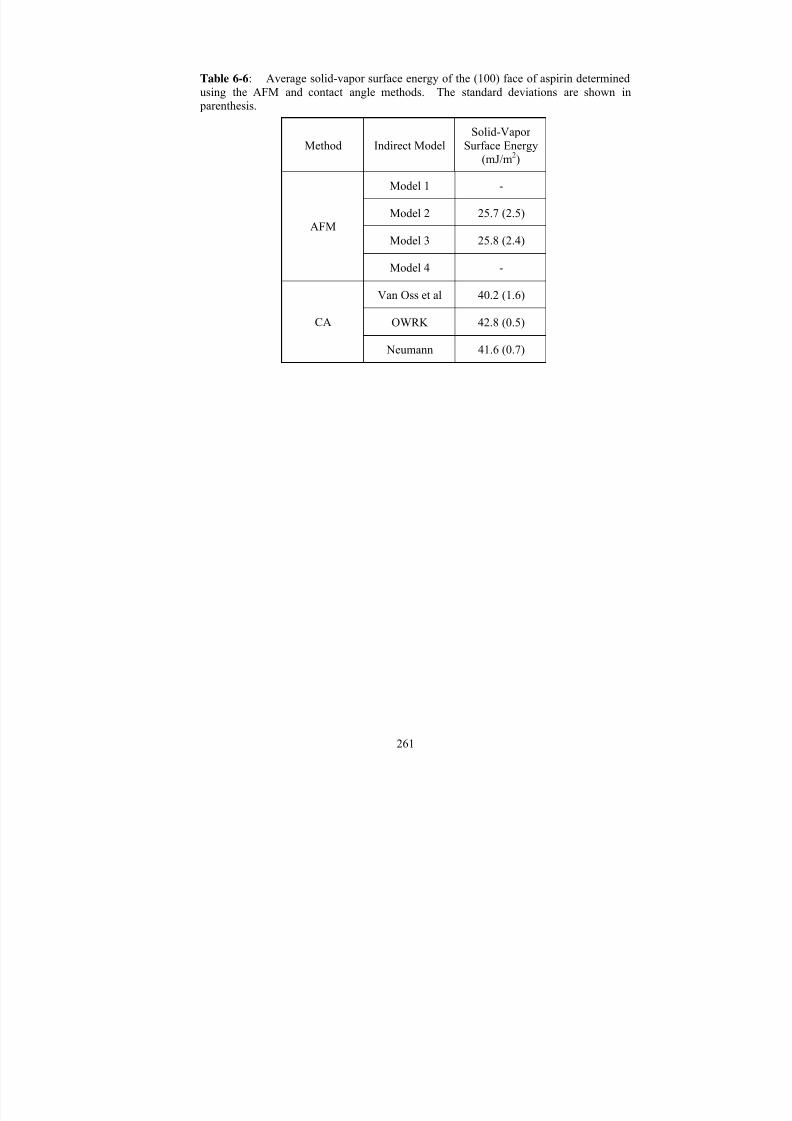
7/27/2019 Atomic Force Microscopy Method Development for Surface Energy Analysis
http://slidepdf.com/reader/full/atomic-force-microscopy-method-development-for-surface-energy-analysis 283/365
261
Table 6-6: Average solid-vapor surface energy of the (100) face of aspirin determinedusing the AFM and contact angle methods. The standard deviations are shown in parenthesis.
Method Indirect Model
Solid-Vapor
Surface Energy(mJ/m2)
Model 1 -
Model 2 25.7 (2.5)
Model 3 25.8 (2.4)AFM
Model 4 -
Van Oss et al 40.2 (1.6)
OWRK 42.8 (0.5)CA
Neumann 41.6 (0.7)

7/27/2019 Atomic Force Microscopy Method Development for Surface Energy Analysis
http://slidepdf.com/reader/full/atomic-force-microscopy-method-development-for-surface-energy-analysis 284/365
262
Table 6-7: Mixed model statistics for AFM Measurements on the (001) face of aspirin ina controlled humidity environment. a) Repeated measures ANOVA for within subjecteffects, b) repeated measures ANOVA for between subjects, and c) the variable thatdemonstrates the largest percentage of variance (001) ASA-controlled RH AFMmeasurements.
Degrees of Freedom
Sum of Square
MeanSquare
F Value p
Location 9 0.60 0.07 1.26 0.32Location*(001) 9 0.28 0.03 0.59 0.79Location*Tip 18 1.47 0.08 1.53 0.19Error 18 0.96 0.05 - -
Degrees of Freedom
Sum of Square
MeanSquare
F Value p
(001) Face 1 0.70 0.70 0.90 0.44Tip 2 4.57 2.29 2.92 0.26Error 2 1.57 0.78 - -
Variable % of the Total % Truncated(001) Face 36.7 36.2Tip -1.3 0.0(001) Face*Tip 35.3 34.8(001) Face*Tip*Location (Error) 29.4 29.0
Total 100.0 100.0
a)
b)
c)
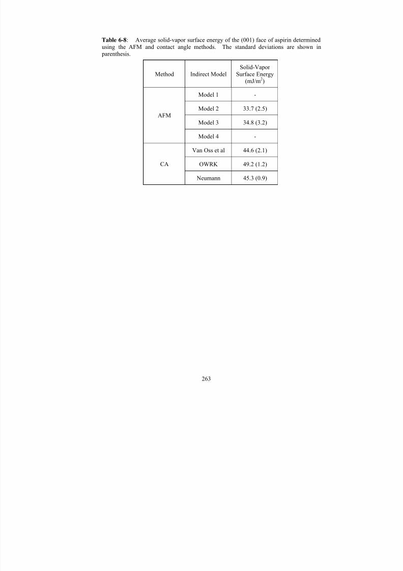
7/27/2019 Atomic Force Microscopy Method Development for Surface Energy Analysis
http://slidepdf.com/reader/full/atomic-force-microscopy-method-development-for-surface-energy-analysis 285/365
263
Table 6-8: Average solid-vapor surface energy of the (001) face of aspirin determinedusing the AFM and contact angle methods. The standard deviations are shown in parenthesis.
Method Indirect Model
Solid-Vapor
Surface Energy(mJ/m2)
Model 1 -
Model 2 33.7 (2.5)
Model 3 34.8 (3.2)AFM
Model 4 -
Van Oss et al 44.6 (2.1)
OWRK 49.2 (1.2)CA
Neumann 45.3 (0.9)

7/27/2019 Atomic Force Microscopy Method Development for Surface Energy Analysis
http://slidepdf.com/reader/full/atomic-force-microscopy-method-development-for-surface-energy-analysis 286/365
264
Figure 6-8: The solid-vapor surface energy from AFM force measurements incontrolled humidity environment on the (001) face of aspirin crystals.
Avera e = 11.3 ± 0.5 nN
Avera e = 58.2 ± 2.2 mN/m
Avera e = 33.7 ± 2.5 mJ/m2
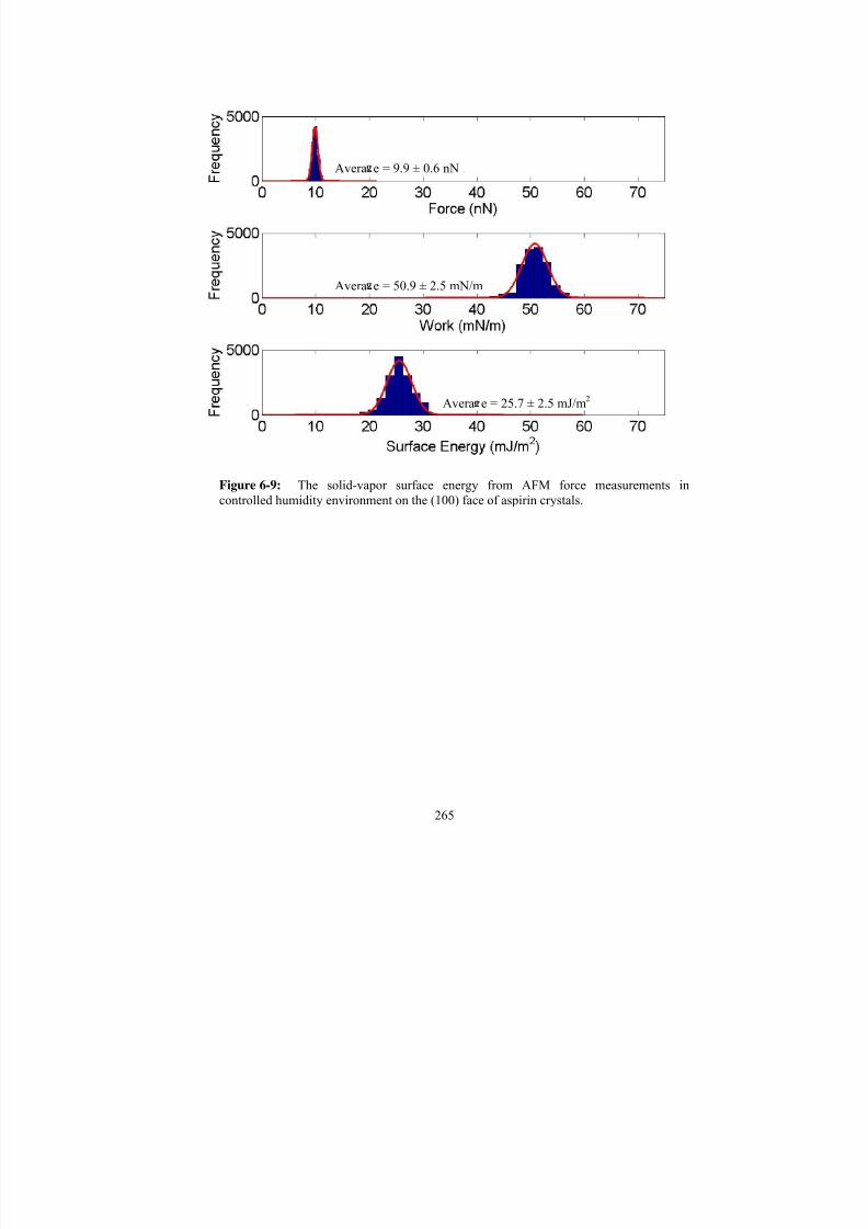
7/27/2019 Atomic Force Microscopy Method Development for Surface Energy Analysis
http://slidepdf.com/reader/full/atomic-force-microscopy-method-development-for-surface-energy-analysis 287/365
265
Figure 6-9: The solid-vapor surface energy from AFM force measurements in
controlled humidity environment on the (100) face of aspirin crystals.
Avera e = 9.9 ± 0.6 nN
Avera e = 50.9 ± 2.5 mN/m
Avera e = 25.7 ± 2.5 mJ/m2

7/27/2019 Atomic Force Microscopy Method Development for Surface Energy Analysis
http://slidepdf.com/reader/full/atomic-force-microscopy-method-development-for-surface-energy-analysis 288/365
266
6.3.2 Solid-liquid surface energy
6.3.2.1 Diiodomethane Solid-Liquid Surface Energy
To determine the solid-liquid surface energy of the (100) and (001) face with
diiodomethane, the spring constants, tip radii, and tip-vapor surface energies were
determined first. Table 6-9 shows the values used to calculate the (100) and (001) solid-
liquiddiiodomethane surface energy.
Force measurements were made on the (100) and (001) surfaces in diiodomethane using
the tip values in Table 6-9. The data was then analyzed in SAS and JMP. The statistics
for the (100) and (001) faces are listed in Table 6-10 and Table 6-12, respectively. The
p values were all greater than 0.05, meaning the null hypotheses was accepted. The p
value for the tips from the force measurements on the (100) face was low (0.08) and thus,
close to being statistically significant. The force range on the (100) face was 0.6 to 0.7
nN. The distribution for each tip was also small with a 0.1 nN standard deviation
(n=5120 per tip). These results indicated the tip variation was negligible. The other
variable with a p value that was close to statistical significance was the locations on the
(001) face. This face was observed to be more rough than the (100) face. Therefore, it
was not surprising that the locations being measured on each crystalline sample would
causing variability. With a standard deviation of 0.3 nN (n=5120), the force distribution
confirmed that location variability was insignificant. The plots of the force, work, and
surface energy of the (100) and (001) faces are shown in Figure 6-10 and Figure 6-11,
respectively.
The forces between the two major faces of aspirin and diiodomethane were expected to
be small. Small forces were indicative of strong adhesion between the sample and the

7/27/2019 Atomic Force Microscopy Method Development for Surface Energy Analysis
http://slidepdf.com/reader/full/atomic-force-microscopy-method-development-for-surface-energy-analysis 289/365
267
liquid. The same was observed from the contact angle measurements. The angle
between the two major faces of aspirin and diiodomethane was smaller than the angles
from water and glycerol. Thus the solid-liquid surface energy was also smaller on these
two faces. The interesting observation between the two methods was the difference
observed from the forces compared to the contact angles. The smallest angle was
measured on the (001) face, Table 6-1, but the smallest force was measured on the (100)
face. However, comparison of the surface energy from contact angle method to the AFM
method indicates that the (100) face has a stronger interaction with diiodomethane.
According to water contact angle measurements, the (100) face was more hydrophobic.The contact angles created a bit of confusion because the largest angles for water and
glycerol are observed on the (100) face. The large angle from liquids with polar
components means the (100) face is more hydrophobic. If the (100) face was more
hydrophobic, a smaller angle from diiodomethane would have been expected. For
contact angle results, the solid-liquid surface energy had to be calculated and the
interaction between the three liquids had to be considered before the stronger
diiodomethane interaction with the (100) face was seen. The AFM does not need
multiple liquids to determine the solid-liquid surface energy. The measurements in the
liquid of interest and surface energy models 2 and 3 are sufficient to calculate solid-liquid
surface energy values directly, making AFM an attractive alternative to contact angle for
surface energy measurements.
To compare the solid-liquid surface energy values of the AFM with contact angle
measurements, the AFM surface-energy models are discussed first. The results from the
(100) and (001) faces of aspirin are listed in Table 6-11 and Table 6-13, respectively.
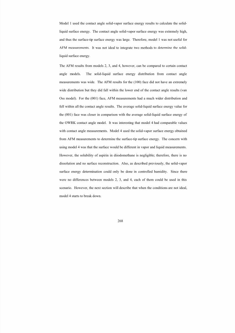
7/27/2019 Atomic Force Microscopy Method Development for Surface Energy Analysis
http://slidepdf.com/reader/full/atomic-force-microscopy-method-development-for-surface-energy-analysis 290/365
268
Model 1 used the contact angle solid-vapor surface energy results to calculate the solid-
liquid surface energy. The contact angle solid-vapor surface energy was extremely high,
and thus the surface-tip surface energy was large. Therefore, model 1 was not useful for
AFM measurements. It was not ideal to integrate two methods to determine the solid-
liquid surface energy.
The AFM results from models 2, 3, and 4, however, can be compared to certain contact
angle models. The solid-liquid surface energy distribution from contact angle
measurements was wide. The AFM results for the (100) face did not have an extremely
wide distribution but they did fall within the lower end of the contact angle results (van
Oss model). For the (001) face, AFM measurements had a much wider distribution and
fell within all the contact angle results. The average solid-liquid surface energy value for
the (001) face was closer in comparison with the average solid-liquid surface energy of
the OWRK contact angle model. It was interesting that model 4 had comparable values
with contact angle measurements. Model 4 used the solid-vapor surface energy obtained
from AFM measurements to determine the surface-tip surface energy. The concern with
using model 4 was that the surface would be different in vapor and liquid measurements.
However, the solubility of aspirin in diiodomethane is negligible; therefore, there is no
dissolution and no surface reconstruction. Also, as described previously, the solid-vapor
surface energy determination could only be done in controlled humidity. Since there
were no differences between models 2, 3, and 4, each of them could be used in this
scenario. However, the next section will describe that when the conditions are not ideal,
model 4 starts to break down.
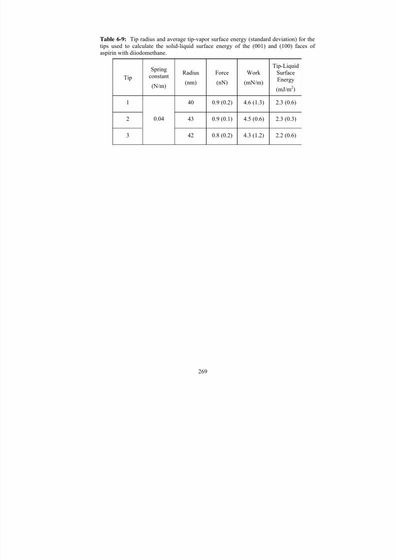
7/27/2019 Atomic Force Microscopy Method Development for Surface Energy Analysis
http://slidepdf.com/reader/full/atomic-force-microscopy-method-development-for-surface-energy-analysis 291/365
269
Table 6-9: Tip radius and average tip-vapor surface energy (standard deviation) for thetips used to calculate the solid-liquid surface energy of the (001) and (100) faces of aspirin with diiodomethane.
Tip
Spring
constant(N/m)
Radius(nm)
Force(nN)
Work (mN/m)
Tip-Liquid
SurfaceEnergy
(mJ/m2)
1 40 0.9 (0.2) 4.6 (1.3) 2.3 (0.6)
2 43 0.9 (0.1) 4.5 (0.6) 2.3 (0.3)
3
0.04
42 0.8 (0.2) 4.3 (1.2) 2.2 (0.6)
7/27/2019 Atomic Force Microscopy Method Development for Surface Energy Analysis
http://slidepdf.com/reader/full/atomic-force-microscopy-method-development-for-surface-energy-analysis 292/365
270
Table 6-10: Mixed model statistics for AFM Measurements on the (100) face of aspirinin diiodomethane. a) Repeated measures ANOVA for within subject effects, b) repeatedmeasures ANOVA for between subjects, and c) the variable that demonstrates the largest percentage of variance (100) ASA-diiodomethane AFM measurements.
Degrees of
Freedom
Sum of
Square
Mean
Square F Value pLocation 9 0.007 0.0008 0.30 0.97Location*(100) 9 0.009 0.001 0.38 0.93Location*Tip 18 0.056 0.003 1.12 0.41Error 18 0.050 0.003 - -
Degrees of Freedom
Sum of Square
MeanSquare
F Value p
(100) Face 1 0.0001 .0001 0.13 0.75Tip 2 0.1243 0.622 12.03 0.08Error 2 0.0103 0.005 - -
Variable % of the Total % TruncatedTip 51.7 50.4(100) Face -2.7 0.0(100) Face*Tip 4.8 4.6(100) Face*Tip*Location (Error) 46.2 45.0
Total 100.0 100.0
a)
b)
c)

7/27/2019 Atomic Force Microscopy Method Development for Surface Energy Analysis
http://slidepdf.com/reader/full/atomic-force-microscopy-method-development-for-surface-energy-analysis 293/365
271
Table 6-11: Average solid-liquid surface energy of the (100) face of aspirin withdiiodomethane determined using the AFM and contact angle methods.
(Note: Contact angle measurements are made in ambient conditions and AFM vapor measurements are done in controlled humidity environment.)
Method ModelSolid-Liquid
Surface Energy
(mJ/m2)
Van Oss et al 15.6 (0.6)
OWRK 18.2 (0.6)Model 1
Neumann 17.0 (0.6)
Model 2 1.2 (0.4)
Model 3 1.2 (0.4)
Model 2 γsv 1.1 (0.6)
AFM
Model 4
Model 3 γsv 1.1 (0.6)
Van Oss et al 1.6 (0.7)
OWRK 4.7 (0.9)Contact
Angle
Neumann 3.3 (0.9)

7/27/2019 Atomic Force Microscopy Method Development for Surface Energy Analysis
http://slidepdf.com/reader/full/atomic-force-microscopy-method-development-for-surface-energy-analysis 294/365
272
Table 6-12: Mixed model statistics for AFM Measurements on the (001) face of aspirinin diiodomethane. a) Repeated measures ANOVA for within subject effects, b) repeatedmeasures ANOVA for between subjects, and c) the variable that demonstrates the largest percentage of variance (001) ASA-diiodomethane AFM measurements.
Degrees of Freedom Sum of Square MeanSquare F Value p
Location 9 0.09 0.011 2.18 0.08Location*(001) 9 0.08 0.009 1.87 0.12Location*Tip 18 0.16 0.008 1.81 0.11Error 18 0.09 0.005 - -
Degrees of Freedom
Sum of Square
MeanSquare
F Value p
(001) Face 1 0.01 0.01 0.6 0.51
Tip 2 0.19 0.10 4.4 0.18Error 2 0.04 0.02 - -
Variable % of the Total % TruncatedTip 30.8 30.1(001) Face -2.2 0.0(001) Face*Tip 11.8 11.5(001) Face*Tip*Location (Error) 59.7 58.4
Total 100.0 100.0
a)
b)
c)

7/27/2019 Atomic Force Microscopy Method Development for Surface Energy Analysis
http://slidepdf.com/reader/full/atomic-force-microscopy-method-development-for-surface-energy-analysis 295/365
273
Table 6-13: Average solid-liquid surface energy of the (001) face of aspirin withdiiodomethane determined using the AFM and contact angle methods.
(Note: Contact angle measurements are made in ambient conditions and AFM vapor measurements are done in controlled humidity environment.)
Method ModelSolid-Liquid
Surface Energy
(mJ/m2)
Van Oss et al 16.8 (1.4)
OWRK 21.4 (1.4)Model 1
Neumann 17.5(1.4)
Model 2 6.4 (2.3)
Model 3 6.6 (2.4)
Model 2 γsv 5.9 (1.4)
AFM
Model 4
Model 3 γsv 7.0 (1.4)
Van Oss et al 2.5 (1.4)
OWRK 7.9 (0.9)Contact
Angle
Neumann 4.3 (0.6)

7/27/2019 Atomic Force Microscopy Method Development for Surface Energy Analysis
http://slidepdf.com/reader/full/atomic-force-microscopy-method-development-for-surface-energy-analysis 296/365
274
Figure 6-10: The solid-liquid surface energy from AFM force measurements withdiiodomethane on the (100) face of aspirin crystals.
Avera e = 0.6 ± 0.1 nN
Avera e = 3.2 ± 0.6 mN/m
Avera e = 1.2 ± 0.4 mJ/m2

7/27/2019 Atomic Force Microscopy Method Development for Surface Energy Analysis
http://slidepdf.com/reader/full/atomic-force-microscopy-method-development-for-surface-energy-analysis 297/365
275
Figure 6-11: The solid-liquid surface energy from AFM force measurements withdiiodomethane on the (001) face of aspirin crystals.
Avera e = 1.5 ± 0.3 nN
Avera e = 7.5 ± 1.4 mN/m
Avera e = 6.4 ± 2.3 mJ/m2

7/27/2019 Atomic Force Microscopy Method Development for Surface Energy Analysis
http://slidepdf.com/reader/full/atomic-force-microscopy-method-development-for-surface-energy-analysis 298/365
276
6.3.2.1 Water Solid-Liquid Surface Energy
Unlike the inert surface, ASA’s solubility in water caused dissolution on the major
surfaces. Therefore, it was hard to control the consistency of the measurements, and it
was difficult to know the specific interaction that was being measured. As a result,
surface energy measurements were captured from ASA crystals immersed in ASA
solutions at various concentrations. The ASA solutions were prepared at concentrations
surrounding 18 mM, the saturation solubility of ASA in water. The presence of the
additive eliminated the possibility for direct comparison with contact angle measurements
with pure water. Additives are known to affect crystal growth; therefore, differences
were expected between the force of adhesion in a pure solvent and a solvent with an
additive. The contact angles cannot be measured in additive solutions because of the risk
of preferential absorption at one of the three interfaces.[16] Therefore, the solid-liquid
surface energy measurements with the AFM were focused towards evaluating the
differences between ASA solutions prepared at different concentrations. The same
principles from Chapter 5 still applied to these experiments.
To determine the solid-liquid surface energy of the (100) and (001) face with varying
concentration of ASA, the spring constants, tip radii, and tip-vapor surface energies were
determined first. Table 6-14 lists the tip properties for each tip used in the 12, 14, 16, 18,
and 20 mM solutions. These values were later used for calculation the solid-liquid
surface energy on the (100) and (001) faces of ASA.
Force measurements were made first on the (100) and (001) surfaces in all five solutions
using the tips in Table 6-14. The data were then analyzed in SAS and JMP. The
statistics for the (001) and (100) faces in a 12mM ASA solution are listed in Table 6-15
7/27/2019 Atomic Force Microscopy Method Development for Surface Energy Analysis
http://slidepdf.com/reader/full/atomic-force-microscopy-method-development-for-surface-energy-analysis 299/365
277
and Table 6-16, respectively. The data could not be combined to calculate an average
force, work, and surface energy because of the p values in Table 6-15a and Table 6-16a
show the results for within subjects, the time intervals. The p values for time were
significantly below 0.05, which meant the values were changing over the time interval
studied. These early results prompted another change in the methodology of measuring
the forces on ASA. Instead of taking measurements quickly in 10 different spots, the
measurements were taken 10 minutes apart until it was confirmed that a steady state had
been reached. When the p values are small and there was no steady state for force
measurements, it was not possible to calculate an average using the entire data set. In thisscenario, an overall average would be misleading. For the measurements in 12mM ASA,
no experimental adjustments could be made to induce a steady-state. Since the 12mM
condition was well below saturation solubility, dissolution of the crystal continued until
equilibrium was reached.
Even though all an overall average for force, work, and surface energy could not be
determined, plots were developed that incorporated the data at each ten minute time
interval. Figure 6-12, Figure 6-13, and Figure 6-14 show the solid-liquid surface
energy from model 1, models 2 and 3, and model 4, respectively. Models 2 and 3 are the
only surface energy equations that apply under conditions where the surface is changing
since they do not rely on solid-vapor surface energy data and do not operate under the
assumption that the surface is unchanged from vapor to liquid measurements. Figure
6-12 showed extremely high solid-liquid surface energy because of the large solid-vapor
surface energy from contact angle. Figure 6-14, showed the lowest solid-liquid surface

7/27/2019 Atomic Force Microscopy Method Development for Surface Energy Analysis
http://slidepdf.com/reader/full/atomic-force-microscopy-method-development-for-surface-energy-analysis 300/365
278
energy, but still relied on a calculated surface-tip surface energy from an unchanged
surface in vapor. Therefore, use of models 2 or 3 was required for these experiments.

7/27/2019 Atomic Force Microscopy Method Development for Surface Energy Analysis
http://slidepdf.com/reader/full/atomic-force-microscopy-method-development-for-surface-energy-analysis 301/365
279
Table 6-14: Tip radius and average tip-vapor surface energy (standard deviation) for thetips used to calculate the solid-liquid surface energy of the (001) and (100) faces of aspirin with 12, 14, 16, 18, and 20mM ASA solutions.
Tip
ASA
SolutionConcentration
(mM)
Springconstant
(N/m)
Radius(nm)
Force(nN)
Work (mN/m)
Tip-Liquid
SurfaceEnergy
(mJ/m2)
1 41 0.5 (0.2) 2.8 (1.1) 1.4 (0.5)
212
40 0.5 (0.1) 2.6 (0.6) 1.3 (0.3)
1 41 0.7 (0.2) 3.4 (1.0) 1.7 (0.5)
214
42 0.7 (0.2) 3.7 (1.1) 1.8 (0.6)
1 40 0.7 (0.3) 4.0 (1.6) 2.0 (0.8)
2 38 0.8 (0.2) 4.5 (1.0) 2.2 (0.5)
3
16
45 0.9 (0.2) 4.3 (0.8) 2.1 (0.4)
1 40 0.7 (0.2) 3.9 (1.1) 2.0 (0.6)
2 41 0.7 (0.1) 3.8 (0.6) 1.9 (0.3)
3
18
39 0.7 (0.1) 3.7 (0.4) 1.9 (0.2)
1 41 0.9 (0.3) 4.4 (1.7) 2.2 (0.9)
2 43 0.8 (0.2) 3.7 (0.8) 1.9 (0.4)
3
20
0.04
40 0.7 (0.2) 4.0 (1.0) 2.0 (0.5)

7/27/2019 Atomic Force Microscopy Method Development for Surface Energy Analysis
http://slidepdf.com/reader/full/atomic-force-microscopy-method-development-for-surface-energy-analysis 302/365
280
Table 6-15: Mixed model statistics for AFM Measurements on the (001) face of aspirinin 12mM ASA Solution. a) Repeated measures ANOVA for within subject effects, b)repeated measures ANOVA for between subjects, and c) the variable that demonstratesthe largest percentage of variance (001) ASA-diiodomethane AFM measurements.
Degrees of Freedom Sum of Square MeanSquare F Value p
Time 5 1.20 0.24 492.69 <0.0001Time*(001) 5 0.09 0.02 36.64 0.0006Time*Tip 5 0.16 0.03 66.68 0.0001Error 5 0.002 0.0005 - -
Degrees of Freedom
Sum of Square
MeanSquare
F Value p
(001) Face 1 0.005 0.005 12.96 0.17
Tip 1 0.252 0.252 605.16 0.03Error 1 0.0004 0.0004 - -
Variable % of the Total % Truncated(001) Face 1.2 1.1Tip 58.9 54.7(001) Face*Tip -7.7 0.0(001) Face*Tip*Time (Error) 47.6 44.2
Total 100.0 100.0
a)
b)
c)

7/27/2019 Atomic Force Microscopy Method Development for Surface Energy Analysis
http://slidepdf.com/reader/full/atomic-force-microscopy-method-development-for-surface-energy-analysis 303/365
281
Table 6-16: Mixed model statistics for AFM Measurements on the (100) face of aspirinin 12mM ASA solution. a) Repeated measures ANOVA for within subject effects, b)repeated measures ANOVA for between subjects, and c) the variable that demonstratesthe largest percentage of variance (001) ASA-diiodomethane AFM measurements.
Degrees of
Freedom
Sum of
Square
Mean
Square F Value pTime 5 0.31 0.06 79.17 <0.0001Time*(100) 5 0.02 0.004 6.24 0.0329Time*Tip 5 0.06 0.01 15.85 0.0044Error 5 0.004 0.0008 - -
Degrees of Freedom
Sum of Square
MeanSquare
F Value p
(100) Face 1 0.03 0.03 68.44 0.08Tip 1 0.07 0.07 133.30 0.06Error 1 0.0005 0.0005 - -
Variable % of the Total % Truncated(100) Face 10.2 9.6Tip 40.6 38.2(100) Face*Tip -6.3 0.0(100) Face*Tip*Time (Error) 55.5 52.2
Total 100.0 100.0
a)
b)
c)

7/27/2019 Atomic Force Microscopy Method Development for Surface Energy Analysis
http://slidepdf.com/reader/full/atomic-force-microscopy-method-development-for-surface-energy-analysis 304/365
282
Figure 6-12: Model 1 solid-liquid surface energy from AFM force measurements using
a 12mM ASA solution on the (001) and (100) faces of aspirin crystals. Model 1 usessolid-vapor contact angle results from a) the van Oss, b) OWRK, and c) Neumannindirect models.
0
5
10
15
20
25
0 10 20 30 40 50 60 70
Time (min)
S u r f a c e E n e r g y ( m J / m
2 )
(001) 12mM ASA (100) 12mM ASA
0
5
10
15
20
25
0 10 20 30 40 50 60 70
Time (min)
S u r f a c e E n e r g y ( m J / m
2 )
(001) 12mM ASA (100) 12mM ASA
a)
b)
c)
0
5
10
15
20
25
0 10 20 30 40 50 60 70
Time (min)
S u r f a c e E n e r g y ( m J / m
2 )
(001) 12mM ASA (100) 12mM ASA

7/27/2019 Atomic Force Microscopy Method Development for Surface Energy Analysis
http://slidepdf.com/reader/full/atomic-force-microscopy-method-development-for-surface-energy-analysis 305/365
283
Figure 6-13: Model 2 and model 3 solid-liquid surface energy from AFM forcemeasurements using a 12mM ASA solution on the (001) and (100) faces of aspirincrystals. Model 2 uses the geometric mean, a), and model 3 uses the modified geometricmean, b).
0
2
4
68
10
12
14
16
0 10 20 30 40 50 60 70
Time (mins)
S u r f a c e E n e r g y ( m J / m
2 )
(001) 12mM ASA (100) 12mM ASA
0
2
4
6
8
10
12
14
16
0 10 20 30 40 50 60 70
Time (min)
S u r f a c e E n e r g y ( m J / m
2 )
(001) 12mM ASA (100) 12mM ASA
a)
b)

7/27/2019 Atomic Force Microscopy Method Development for Surface Energy Analysis
http://slidepdf.com/reader/full/atomic-force-microscopy-method-development-for-surface-energy-analysis 306/365

7/27/2019 Atomic Force Microscopy Method Development for Surface Energy Analysis
http://slidepdf.com/reader/full/atomic-force-microscopy-method-development-for-surface-energy-analysis 307/365
285
The data from the 14mM ASA solutions was similar to the 12 mM. The statistics in
Table 6-17 and Table 6-18 show the p values of the times within subjects are
significantly smaller than 0.05. Hence, the null hypothesis must be rejected and an
average force, work, and surface energy with the entire data set was not calculated.
However, the times' p values have gone up and are closer to the required 0.05, the
significance level set for accepting or rejecting the null hypothesis. Therefore, the
environmental conditions were improved as compared to the 12mM solution. In 14mM
solutions, the data could not be combined and instead was plotted to show the changes
over time in Figure 6-15, Figure 6-16, and Figure 6-17.
Figure 6-15 shows the results from model 1, which used contact angle based solid-vapor
surface energy values. These values were higher than the contact angle results and
mostly reflected the large values of the calculated surface-tip surface energy. The results
from surface energy model 4 are shown in Figure 6-17. Since the forces were still
changing over time, this model was also not ideal for determining surface energy because
the assumption cannot be made that the surface in vapor was the same as it was in liquid.
Therefore, model 2 and 3 are best suited for determining solid-liquid surface energy.
The modification in model 3 was not necessary when the interaction of the two separate
phases were similar. Therefore, model 2 can be used to calculate the surface energy.
There are three important observations that need to be pointed out from the 12mM and
14mM ASA solution results. First, at the 10 minute time point, the solid-liquid surface
energy was high, similar to the results obtained from contact angle measurements. Over
time, the surface energy decreased, indicating a more favorable interaction between the
solution and the surface of the aspirin crystal. This could be due to the exchange of

7/27/2019 Atomic Force Microscopy Method Development for Surface Energy Analysis
http://slidepdf.com/reader/full/atomic-force-microscopy-method-development-for-surface-energy-analysis 308/365
286
molecules at the surface until an equilibrium state was reached. The second observation
was the smaller solid-liquid surface energy on the (100) face than the (001) face in
models 2, 3, and 4. Model 1 was the only surface energy model that required knowledge
of the solid-vapor surface energy a priori. The trend was the reversed from contact angle
measurements where the (001) face had a smaller solid-liquid surface energy. During
AFM measurements, it was possible that dissolution on the (100) face revealed the
carboxylic acid. If this chemical moiety was revealed, the surface was more hydrophilic,
resulting in a stronger interaction with water and a smaller surface energy. The high
sensitivity of the AFM probes made it possible to distinguish between chemical moieties.This was not possible with contact angle measurements since they are conducted at the
macroscopic scale. In all cases, the angles measured on the (100) face with water were
larger than those on the (001) face. The AFM measurements have helped gain critical
knowledge about the effects of environment and additive concentration on surface
energy. These results may be more beneficial than just looking at pure solvents because
the actual crystallization environment is under direct investigation.
Since a true average surface energy value was not calculated from the data because a
steady state was not reached under these conditions, the JMP data was not relevant. The
JMP data helped to understand the variation between subjects, the sample, the tips, the
interaction of the tip with the sample in a certain environmental conditions, and the
overall residual error. However, the JMP data did not consider time variability because
the entire use of repeated measures mixed model broke down when there is time
variability. When the statistical variance between times was not equal, the null
hypothesis was rejected. In this instance, the experimental methodology needed to be

7/27/2019 Atomic Force Microscopy Method Development for Surface Energy Analysis
http://slidepdf.com/reader/full/atomic-force-microscopy-method-development-for-surface-energy-analysis 309/365
287
reconsidered and modified to find a condition where times within the subjects did not
change. To do this, the aspirin concentration was increased to 16mM.
During these measurements, the degradation of aspirin was not monitored or evaluated.
Aspirin is known to degrade to salicylic acid and the pH of the solution was not
controlled to stop or slow the degradation. Therefore, it is also possible, in the solutions
below saturation, that the liquid injected for measurements had a mixture of salicylic acid
and aspirin. The purpose of these measurements was to find a point when dissolution on
the surface was minimized and a constant surface energy could be measured. Hence, this
study will not report the degradation of aspirin to salicylic acid.

7/27/2019 Atomic Force Microscopy Method Development for Surface Energy Analysis
http://slidepdf.com/reader/full/atomic-force-microscopy-method-development-for-surface-energy-analysis 310/365
288
Table 6-17: Mixed model statistics for AFM Measurements on the (001) face of aspirinin 14mM ASA Solution. a) Repeated measures ANOVA for within subject effects, b)repeated measures ANOVA for between subjects, and c) the variable that demonstratesthe largest percentage of variance (001) ASA-diiodomethane AFM measurements.
Degrees of
Freedom
Sum of
Square
Mean
Square F Value pTime 5 1.10 0.22 13.26 0.007Time*(001) 5 0.24 0.05 2.94 0.13Time*Tip 5 0.11 0.022 1.38 0.37Error 5 0.08 0.02 - -
Degrees of Freedom
Sum of Square
MeanSquare
F Value p
(001) Face 1 0.12 0.12 2.80 0.34Tip 1 0.09 0.09 2.12 0.38Error 1 0.04 0.04 - -
Variable % of the Total % Truncated(001) Face 16.6 16.6Tip 6.8 6.8(001) Face*Tip 4.2 4.2(001) Face*Tip*Time (Error) 72.4 72.4
Total 100.0 100.0
a)
b)
c)

7/27/2019 Atomic Force Microscopy Method Development for Surface Energy Analysis
http://slidepdf.com/reader/full/atomic-force-microscopy-method-development-for-surface-energy-analysis 311/365
289
Table 6-18: Mixed model statistics for AFM Measurements on the (100) face of aspirinin 14mM ASA solution. a) Repeated measures ANOVA for within subject effects, b)repeated measures ANOVA for between subjects, and c) the variable that demonstratesthe largest percentage of variance (001) ASA-diiodomethane AFM measurements.
Degrees of
Freedom
Sum of
Square
Mean
Square F Value pTime 5 1.33 0.27 54.94 0.0002Time*(100) 5 0.04 0.009 1.87 0.25Time*Tip 5 0.05 0.01 2.06 0.22Error 5 0.24 0.005 - -
Degrees of Freedom
Sum of Square
MeanSquare
F Value p
(100) Face 1 0.0007 0.0007 0.02 0.91Tip 1 0.005 0.005 0.16 0.76Error 1 0.03 0.03 - -
Variable % of the Total % Truncated(100) Face -28.8 0.0Tip -22.6 0.0(100) Face*Tip 39.2 25.9(100) Face*Tip*Time (Error) 112.3 74.1
Total 100.0 100.0
a)
b)
c)

7/27/2019 Atomic Force Microscopy Method Development for Surface Energy Analysis
http://slidepdf.com/reader/full/atomic-force-microscopy-method-development-for-surface-energy-analysis 312/365
290
Figure 6-15: Model 1 solid-liquid surface energy from AFM force measurements usinga 14mM ASA solution on the (001) and (100) faces of aspirin crystals. Model 1 usessolid-vapor contact angle results from a) the van Oss, b) OWRK, and c) Neumannindirect models.
0.0
5.0
10.0
15.0
20.0
25.0
0 10 20 30 40 50 60 70
Time (min)
S u r f a c e
E n e r g y ( m J / m
2 )
(001) ASA 14mM (100) ASA 14mM
0.0
5.0
10.0
15.0
20.0
25.0
0 10 20 30 40 50 60 70
Time (min)
S u r f a c e E n e r g y ( m J / m
2 )
(001) ASA 14mM (100) ASA 14mM
0.0
5.0
10.0
15.0
20.0
25.0
0 10 20 30 40 50 60 70
Time (min)
S u r f a c e E n e r g y ( m J / m
2 )
(001) ASA 14mM (100) ASA 14mM
a)
b)
c)

7/27/2019 Atomic Force Microscopy Method Development for Surface Energy Analysis
http://slidepdf.com/reader/full/atomic-force-microscopy-method-development-for-surface-energy-analysis 313/365
291
Figure 6-16: Model 2 and model 3 solid-liquid surface energy from AFM forcemeasurements using a 14mM ASA solution on the (001) and (100) faces of aspirincrystals. Model 2 uses the geometric mean, a), and model 3 uses the modified geometricmean, b).
0.0
2.0
4.0
6.0
8.0
10.0
12.0
14.0
0 10 20 30 40 50 60 70
Time (min)
S u r f a c e E n
e r g y ( m J / m
2 )
(001) ASA 14mM (100) ASA 14mM
0.0
2.0
4.0
6.0
8.0
10.0
12.0
14.0
0 10 20 30 40 50 60 70
Time (min)
S u r f a c e E n e r g y ( m J / m
2 )
(001) ASA 14mM (100) ASA 14mM
a)
b)

7/27/2019 Atomic Force Microscopy Method Development for Surface Energy Analysis
http://slidepdf.com/reader/full/atomic-force-microscopy-method-development-for-surface-energy-analysis 314/365
292
Figure 6-17: Model 4 solid-liquid surface energy from AFM force measurements usinga 14mM ASA solution on the (001) and (100) faces of aspirin crystals.
0.0
2.0
4.0
6.0
8.0
10.0
12.0
14.0
0 10 20 30 40 50 60 70
Time (min)
S u r f a c e E n e r
g y ( m J / m
2 )
(001) ASA 14mM (100) ASA 14mM
0.0
2.0
4.0
6.0
8.0
10.0
12.0
14.0
0 10 20 30 40 50 60 70
Time (min)
S u r f a c e E n e r g y ( m J / m
2 )
(001) ASA 14mM (100) ASA 14mM
a)
b)

7/27/2019 Atomic Force Microscopy Method Development for Surface Energy Analysis
http://slidepdf.com/reader/full/atomic-force-microscopy-method-development-for-surface-energy-analysis 315/365
293
The force measurements were made in a 16mM ASA solution and then analyzed with the
statistical repeated measures mixed model. The SAS and JMP statistics are shown in
Table 6-19 and Table 6-20. The p values within subjects and between subjects are all
above 0.05; therefore, the null hypothesis was accepted and the data was combined to
calculate an average force, work, and surface energy. This was the first aqueous additive
condition that did not show changes over time. The 16mM solution was about 2mM
under the ASA saturation solubility in water. The first force measurements were not
made until 10 minutes after the solution has been injected. It was observed when
measuring the forces in liquids on inert surfaces that an "equilibrium" period wasnecessary to eliminate some of the variation. The "equilibrium" period began from the
moment the liquid was injected onto the surface until little to no variability was observed
between the force measurements at one spot or at different locations. Since the
"equilibrium" period was required for the inert surfaces, it was applied to the crystalline
material as well. In the 12mM and 14mM solutions, each 10 minute interval brought
about a measurable change in solid-liquid surface energy. Thus, it can be assumed that
between 0 and 10 minutes, there was also a reduction in surface energy. Dissolution on
the crystalline surface could have occurred on this time scale at the 16mM condition to
bring the solution’s concentration up to 18 mM, which would explain the apparent steady
state.
The average force, work, and surface energy for the (001) and (100) faces are shown in
Figure 6-18. From the previous measurements in a 14mM solution, the final surface
energy on the (001) face was about 2 mJ/m2. The average solid-vapor surface energy in
16mM was about 2.6 mJ/m2. For the (100) face, the average for the final solid-liquid

7/27/2019 Atomic Force Microscopy Method Development for Surface Energy Analysis
http://slidepdf.com/reader/full/atomic-force-microscopy-method-development-for-surface-energy-analysis 316/365
294
surface energy measurement in 14mM was 0.9 mJ/m2 and the average solid-liquid
surface energy for the 16mM solution was 1.0 mJ/m2. Therefore, it seems the decrease in
surface energy is starting to level off and the dissolution has slowed down or stopped on
both of the faces.
In Table 6-21, the average solid-liquid surface energy values for the (100) and (001)
faces of aspirin are listed for the four AFM surface energy models side by side with the
contact angle measurements. The results calculated with model 1 were still higher than
those determined by contact angle measurements. The use of contact angles to determine
surface-tip surface energy was unreliable when an additive solution was used. The ASA
and water molecules interacted with the surface molecules, causing reorientation,
dissolution, and crystallization. With all of these changes, the assumption that the surface
and the surface-tip surface energy remained identical is likely invalid. The assumption is
applied to both models 1 and 4, and even though model 4 used only AFM data, the
changes occurring on the surface caused concern for the applicability of these models.
Therefore, it is thought that the results from models 2 and 3 were more reliable. These
two models only required AFM data, and the similarities of the geometric mean and the
modified geometric mean results confirmed the use of the geometric mean. The
modification did not change the surface energy, which showed the geometric mean could
be used. The geometric mean was developed for van der Waals interactions, and
therefore, can be used due to the chemical moieties present on the surface of the (100)
and (001) faces. The reduction in the surface energy from the 12mM to 16mM solution
showed that the AFM was sensitive enough to detect differences in the environmental
conditions which could be quantified by model 2. However, if the carboxylic acid was

7/27/2019 Atomic Force Microscopy Method Development for Surface Energy Analysis
http://slidepdf.com/reader/full/atomic-force-microscopy-method-development-for-surface-energy-analysis 317/365
295
revealed on the (100) face the geometric mean may be over or under estimate the surface
energy. The similarities between models 2 and 3 help to justify the use of the geometric
mean for any interactions other than van der Waals. To restate, the difference in the
forces of the individual phases is similar enough to reduce the exponential to one, leaving
only the geometric mean.

7/27/2019 Atomic Force Microscopy Method Development for Surface Energy Analysis
http://slidepdf.com/reader/full/atomic-force-microscopy-method-development-for-surface-energy-analysis 318/365

7/27/2019 Atomic Force Microscopy Method Development for Surface Energy Analysis
http://slidepdf.com/reader/full/atomic-force-microscopy-method-development-for-surface-energy-analysis 319/365
297
Table 6-20: Mixed model statistics for AFM Measurements on the (100) face of aspirinin 16mM ASA solution. a) Repeated measures ANOVA for within subject effects, b)repeated measures ANOVA for between subjects, and c) the variable that demonstratesthe largest percentage of variance (001) ASA-diiodomethane AFM measurements.
Degrees of
Freedom
Sum of
Square
Mean
Square F Value pTime 5 0.01 0.002 0.85 0.54Time*(100) 5 0.003 0.0006 0.21 0.95Time*Tip 10 0.02 0.002 0.72 0.69Error 10 0.03 0.003 - -
Degrees of Freedom
Sum of Square
MeanSquare
F Value p
(100) Face 1 0.001 0.001 1.71 0.32Tip 2 0.010 0.005 8.19 0.11Error 2 0.001 0.0006 - -
Variable % of the Total % Truncated(100) Face 1.9 1.7Tip 22.9 20.2(100) Face*Tip -13.6 0.0(100) Face*Tip*Time (Error) 88.8 78.1
Total 100.0 100.0
a)
b)
c)

7/27/2019 Atomic Force Microscopy Method Development for Surface Energy Analysis
http://slidepdf.com/reader/full/atomic-force-microscopy-method-development-for-surface-energy-analysis 320/365
298
Figure 6-18: The solid-liquid surface energy from AFM force measurements with
16mM ASA solution on the (001) face of aspirin crystals.
Avera e = 0.8 ± 0.2 nN
Avera e = 4.2 ± 1.3 mN/m
Avera e = 2.6 ± 2.3 mJ/m2

7/27/2019 Atomic Force Microscopy Method Development for Surface Energy Analysis
http://slidepdf.com/reader/full/atomic-force-microscopy-method-development-for-surface-energy-analysis 321/365
299
Figure 6-19: The solid-liquid surface energy from AFM force measurements with
16mM ASA solution on the (100) face of aspirin crystals.
Avera e = 0.5 ± 0.1 nN
Avera e = 2.8 ± 0.6 mN/m
Avera e = 1.0 ± 0.4 mJ/m2

7/27/2019 Atomic Force Microscopy Method Development for Surface Energy Analysis
http://slidepdf.com/reader/full/atomic-force-microscopy-method-development-for-surface-energy-analysis 322/365
300
Table 6-21: Average solid-liquid surface energy of the (001) and (100) faces of aspirinwith 16mM ASA solution determined using the AFM and contact angle methods.
(Note: Contact angle measurements are made in ambient conditions and AFMmeasurements are done in controlled humidity environment.)
Method Model
(001)
Solid-Liquid
Surface Energy
mJ/m2
(100)
Solid-Liquid
Surface Energy
mJ/m2
Van Oss et al 13.9 (1.3) 15.3 (0.6)
OWRK 18.5 (1.3) 17.9 (0.6)Model 1
Neumann 14.6 (1.3) 16.7 (0.6)
Model 2 2.6 (2.3) 1.0 (0.4)
Model 3 2.6 (2.6) 1.0 (0.4)
Model 2 γsv 3.0 (1.3) 0.8 (0.6)
AFM
Model 4Model 3 γsv 4.1 (1.3) 0.9 (0.6)
Van Oss et al 3.2 (2.4) 11.3 (3.2)
OWRK 8.6 (1.6) 14.4 (2.4)Contact
Angle
Neumann 5.1 (1.1) 13.0 (2.6)

7/27/2019 Atomic Force Microscopy Method Development for Surface Energy Analysis
http://slidepdf.com/reader/full/atomic-force-microscopy-method-development-for-surface-energy-analysis 323/365
301
No changes were observed in forces over time using the 16mM solutions. Thus, when
using an 18mM and 20mM solution, it was hypothesized that the forces would not vary
over time. It was thought that the 18mM solution would show similar results to the
16mM solution and the 20mM solution would lower the surface energy even more
because it would create a supersaturated condition. In this supersaturated condition, the
solid-liquid surface energy should be strong on the (100) and (001) faces since these are
the two major faces of ASA. By definition, a major face must grow the slowest.
Therefore, more work was required to separate either the additive or water molecule that
blocks the solute molecules from binding to that face and increasing the crystal growth
rate of that face.
As always, the forces were measured first in the 18mM and 20mM solutions. The
statistics for the 18mM solution measurements on the (001) and (100) are listed in Table
6-22 and Table 6-23, respectively. The statistics for the 20mM solution measurements
on the (001) and (100) faces are listed in Table 6-25 and Table 6-26, respectively. The
p values for within and between subjects on both faces and in both conditions were
greater than 0.05. The null hypothesis was accepted and the data was collated so that an
average force, work, and surface energy could be calculated and plotted together. The
force, work, and surface energy results for the (001) and (100) faces with 18mM ASA
solution are shown in Figure 6-20 and Figure 6-21, respectively. Figure 6-22 and
Figure 6-23 illustrate the force, work, and surface energy results for the (001) and (100)
faces in a 20mM ASA solution.
As for the surface energy models used to determine solid-liquid surface energy, models 2
and 3 were still the best choice. Model 1, which requires the use of contact angle

7/27/2019 Atomic Force Microscopy Method Development for Surface Energy Analysis
http://slidepdf.com/reader/full/atomic-force-microscopy-method-development-for-surface-energy-analysis 324/365
302
measurements, still output higher values than the contact angle results for both 18mM
and 20mM ASA solutions. There were still changes in the solid-liquid surface energy
values as compared with other ASA solutions because it was still a dynamic environment.
Since the surface was succeptible to environmental conditions, models 1 and 4 were
invalid. Determining the surface energy in a kinetic condition does not uphold the
assumption that the surface in vapor and surface in liquid remain identical. Also, when
using model 4 for the 20mM solution, a negative value was obtained on the (100) surface.
Once the forces and consequently the work of adhesion in the liquid become smaller than
the tip-liquid surface energy, the solid-liquid surface energy becomes negative.Consequently, like Young's equation for contact angle surface energy determination,
model 4 cannot be used when there is a stronger interaction between a sample and the
environment. This leaves model 2 and 3. The results between the two models on both
faces and from both solutions showed similarities between models 2 and 3. These
similarities have been consistent throughout the entire study. There was no indication
that model 3 was better than model 2. To eliminate the reliance on β from contact angle
measurements, model 2 was chosen as the best model for determining solid-liquid surface
energy, even if the surface had interactions other than van der Waals.
As hypothesized, the model 2 results with the 18mM solution were comparable to the
results from the 16mM, but only on the (100) face. Since there was no statistical
difference over time with the 16mM ASA solution, it was thought that saturation was
reached. Based on ASA solubility, the 18 mM solution was at saturation once it was
injected. There was a small difference between the (001) face in 16 mM and 18 mM.
The results in the 18mM solution indicate equivalent surface energies between the (100)

7/27/2019 Atomic Force Microscopy Method Development for Surface Energy Analysis
http://slidepdf.com/reader/full/atomic-force-microscopy-method-development-for-surface-energy-analysis 325/365
303
and (001) faces, likely due to the fact that they are both major faces and the solution was
saturated. The saturation of the environment has created an equilibrium between the
surface and the liquid on both faces, and since both are major faces the solid-liquid
surface energies are the same.
This observation changes in the 20mM solution. The 20mM solution was a
supersaturated condition, which becomes a driving force for crystallization. The decrease
in forces on both faces indicated the possibility that crystallization was occurring.
Although it was not statistically significant, the average solid-liquid surface energy from
model 2 on the (001) face was still larger than values on the (100) face. While the
contact angle indicated a stronger interaction on the (001) face, it made more sense
scientifically that a stronger interaction would be seen on the (100) face. This stronger
interaction could be because the carboxylic group is present, but it also could be because
the (100) face is larger than the (001) face. Hence, it was growing the slowest out of the
two. If a face grows the slowest, it is possible that interactions between solvents or
additives with the surface are blocking more solute molecules from adhering to that face.
The measured force of adhesion on both faces was small indicating a stronger interaction
with the solution and subsequently a small surface energy.

7/27/2019 Atomic Force Microscopy Method Development for Surface Energy Analysis
http://slidepdf.com/reader/full/atomic-force-microscopy-method-development-for-surface-energy-analysis 326/365
304
Table 6-22: Mixed model statistics for AFM Measurements on the (001) face of aspirinin 18mM ASA Solution. a) Repeated measures ANOVA for within subject effects, b)repeated measures ANOVA for between subjects, and c) the variable that demonstratesthe largest percentage of variance (001) ASA-diiodomethane AFM measurements.
Degrees of
Freedom
Sum of
Square
Mean
Square F Value pTime 5 0.009 0.0018 0.97 0.48Time*(001) 5 0.002 0.0003 0.16 0.97Time*Tip 10 0.011 0.0011 0.57 0.80Error 10 0.019 0.0019 - -
Degrees of Freedom
Sum of Square
MeanSquare
F Value P
(001) Face 1 0.006 0.0064 10.11 0.09Tip 2 0.010 0.0050 7.95 0.11Error 2 0.001 0.0006 - -
Variable % of the Total % Truncated(001) Face 17.3 16.4Tip 19.9 18.8(001) Face*Tip -5.7 0.0(001) Face*Tip*Time (Error) 68.5 64.8
Total 100.0 100.0
a)
b)
c)

7/27/2019 Atomic Force Microscopy Method Development for Surface Energy Analysis
http://slidepdf.com/reader/full/atomic-force-microscopy-method-development-for-surface-energy-analysis 327/365
305
Table 6-23: Mixed model statistics for AFM Measurements on the (100) face of aspirinin 18mM ASA solution. a) Repeated measures ANOVA for within subject effects, b)repeated measures ANOVA for between subjects, and c) the variable that demonstratesthe largest percentage of variance (001) ASA-diiodomethane AFM measurements.
Degrees of
Freedom
Sum of
Square
Mean
Square F Value pTime 5 0.009 0.0018 1.15 0.40Time*(100) 5 0.004 0.0009 0.56 0.73Time*Tip 10 0.006 0.0006 0.42 0.91Error 10 0.150 0.0015 - -
Degrees of Freedom
Sum of Square
MeanSquare
F Value P
(100) Face 1 0.0008 0.0008 0.16 0.72Tip 2 0.0164 0.0082 1.68 0.37Error 2 0.0098 0.0049 - -
Variable % of the Total % Truncated(100) Face -13.1 0.0Tip 15.8 14.0(100) Face*Tip 36.8 32.5(100) Face*Tip*Time (Error) 60.5 53.5
Total 100.0 100.0
a)
b)
c)

7/27/2019 Atomic Force Microscopy Method Development for Surface Energy Analysis
http://slidepdf.com/reader/full/atomic-force-microscopy-method-development-for-surface-energy-analysis 328/365
306
Figure 6-20: The solid-liquid surface energy from AFM force measurements with18mM ASA solution on the (001) face of aspirin crystals.
Avera e = 0.6 ± 0.1 nN
Avera e = 3.1 ± 0.5 mN/m
Avera e = 1.2 ± 0.6 mJ/m2
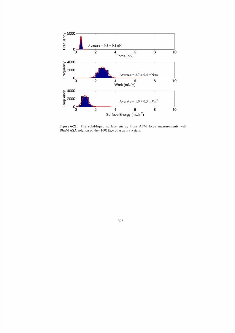
7/27/2019 Atomic Force Microscopy Method Development for Surface Energy Analysis
http://slidepdf.com/reader/full/atomic-force-microscopy-method-development-for-surface-energy-analysis 329/365
307
Figure 6-21: The solid-liquid surface energy from AFM force measurements with18mM ASA solution on the (100) face of aspirin crystals.
Avera e = 0.5 ± 0.1 nN
Avera e = 2.7 ± 0.4 mN/m
Avera e = 1.0 ± 0.3 mJ/m2
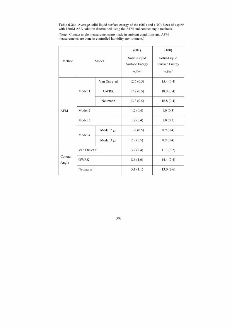
7/27/2019 Atomic Force Microscopy Method Development for Surface Energy Analysis
http://slidepdf.com/reader/full/atomic-force-microscopy-method-development-for-surface-energy-analysis 330/365
308
Table 6-24: Average solid-liquid surface energy of the (001) and (100) faces of aspirinwith 18mM ASA solution determined using the AFM and contact angle methods.
(Note: Contact angle measurements are made in ambient conditions and AFMmeasurements are done in controlled humidity environment.)
Method Model
(001)
Solid-Liquid
Surface Energy
mJ/m2
(100)
Solid-Liquid
Surface Energy
mJ/m2
Van Oss et al 12.6 (0.5) 15.4 (0.4)
OWRK 17.2 (0.5) 18.0 (0.4)Model 1
Neumann 13.3 (0.5) 16.8 (0.4)
Model 2 1.2 (0.4) 1.0 (0.3)
Model 3 1.2 (0.4) 1.0 (0.3)
Model 2 γsv 1.72 (0.5) 0.9 (0.4)
AFM
Model 4
Model 3 γsv 2.9 (0.5) 0.9 (0.4)
Van Oss et al 3.2 (2.4) 11.3 (3.2)
OWRK 8.6 (1.6) 14.4 (2.4)Contact
Angle
Neumann 5.1 (1.1) 13.0 (2.6)

7/27/2019 Atomic Force Microscopy Method Development for Surface Energy Analysis
http://slidepdf.com/reader/full/atomic-force-microscopy-method-development-for-surface-energy-analysis 331/365
309
Table 6-25: Mixed model statistics for AFM Measurements on the (001) face of aspirinin 20mM ASA Solution. a) Repeated measures ANOVA for within subject effects, b)repeated measures ANOVA for between subjects, and c) the variable that demonstratesthe largest percentage of variance (001) ASA-diiodomethane AFM measurements.
Degrees of Freedom Sum of Square MeanSquare F Value p
Time 5 0.0008 0.00017 0.47 0.79Time*(001) 5 0.0008 0.00016 0.46 0.80Time*Tip 10 0.0007 0.00007 0.20 0.99Error 10 0.0036 0.00036 - -
Degrees of Freedom
Sum of Square
MeanSquare
F Value p
(001) Face 1 0.0003 0.00028 4.00 0.18
Tip 2 0.0005 0.00022 3.24 0.24Error 2 0.0001 0.00007 - -
Variable % of the Total % Truncated(001) Face 5.6 5.0Tip 6.3 5.7(001) Face*Tip -10.9 0.0(001) Face*Tip*Time (Error) 99.0 89.3
Total 100.0 100.0
a)
b)
c)
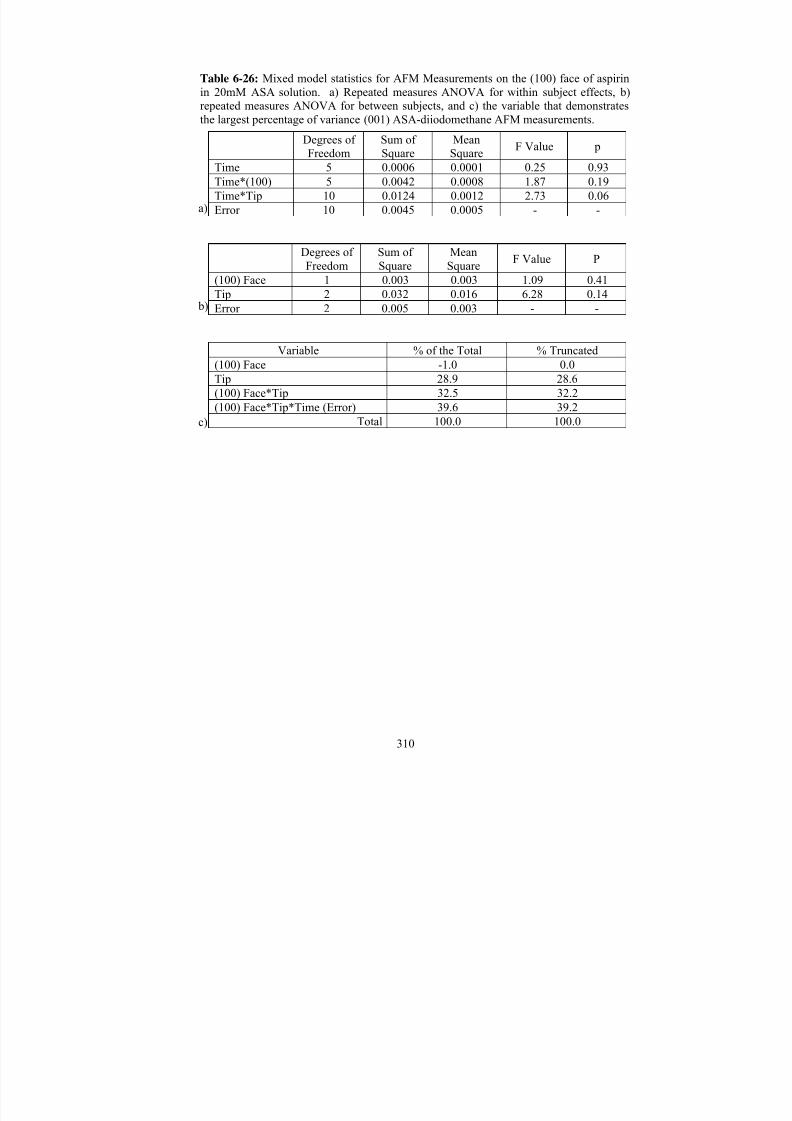
7/27/2019 Atomic Force Microscopy Method Development for Surface Energy Analysis
http://slidepdf.com/reader/full/atomic-force-microscopy-method-development-for-surface-energy-analysis 332/365
310
Table 6-26: Mixed model statistics for AFM Measurements on the (100) face of aspirinin 20mM ASA solution. a) Repeated measures ANOVA for within subject effects, b)repeated measures ANOVA for between subjects, and c) the variable that demonstratesthe largest percentage of variance (001) ASA-diiodomethane AFM measurements.
Degrees of
Freedom
Sum of
Square
Mean
Square F Value pTime 5 0.0006 0.0001 0.25 0.93Time*(100) 5 0.0042 0.0008 1.87 0.19Time*Tip 10 0.0124 0.0012 2.73 0.06Error 10 0.0045 0.0005 - -
Degrees of Freedom
Sum of Square
MeanSquare
F Value P
(100) Face 1 0.003 0.003 1.09 0.41Tip 2 0.032 0.016 6.28 0.14Error 2 0.005 0.003 - -
Variable % of the Total % Truncated(100) Face -1.0 0.0Tip 28.9 28.6(100) Face*Tip 32.5 32.2(100) Face*Tip*Time (Error) 39.6 39.2
Total 100.0 100.0
a)
b)
c)

7/27/2019 Atomic Force Microscopy Method Development for Surface Energy Analysis
http://slidepdf.com/reader/full/atomic-force-microscopy-method-development-for-surface-energy-analysis 333/365
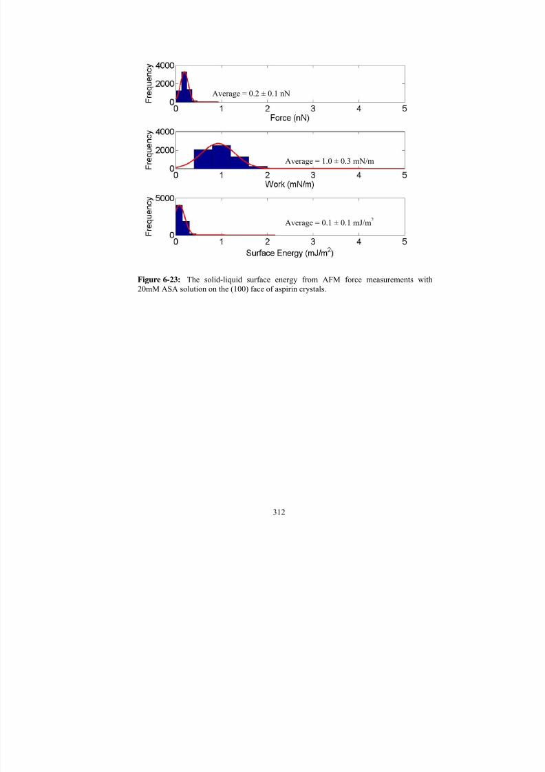
7/27/2019 Atomic Force Microscopy Method Development for Surface Energy Analysis
http://slidepdf.com/reader/full/atomic-force-microscopy-method-development-for-surface-energy-analysis 334/365
312
Figure 6-23: The solid-liquid surface energy from AFM force measurements with20mM ASA solution on the (100) face of aspirin crystals.
Average = 0.2 ± 0.1 nN
Average = 1.0 ± 0.3 mN/m
Average = 0.1 ± 0.1 mJ/m2

7/27/2019 Atomic Force Microscopy Method Development for Surface Energy Analysis
http://slidepdf.com/reader/full/atomic-force-microscopy-method-development-for-surface-energy-analysis 335/365
313
Table 6-27: Average solid-liquid surface energy of the (001) and (100) faces of aspirinwith 20mM ASA solution determined using the AFM and contact angle methods.
(Note: Contact angle measurements are made in ambient conditions and AFMmeasurements are done in controlled humidity environment.)
Method Model
(001)
Solid-Liquid
Surface Energy
mJ/m2
(100)
Solid-Liquid
Surface Energy
mJ/m2
Van Oss et al 11.0 (0.4) 13.5 (0.4)
OWRK 15.6 (0.4) 16.1 (0.4)Model 1
Neumann 11.7 (0.4) 14.9 (0.4)
Model 2 0.3 (0.1) 0.2 (0.1)
Model 3 0.3 (0.1) 0.1 (0.1)
Model 2 γsv 0.1 (0.4) -1.0 (0.4)
AFM
Model 4Model 3 γsv 1.2 (0.4) -1.0 (0.4)
Van Oss et al 3.2 (2.4) 11.3 (3.2)
OWRK 8.6 (1.6) 14.4 (2.4)Contact
Angle
Neumann 5.1 (1.1) 13.0 (2.6)

7/27/2019 Atomic Force Microscopy Method Development for Surface Energy Analysis
http://slidepdf.com/reader/full/atomic-force-microscopy-method-development-for-surface-energy-analysis 336/365
314
6.4 Summary
Several observations were made when the AFM methodology was applied to a crystalline
material. First, there were experimental challenges between contact angle and AFM
measurements. There were substantial differences observed between solid-vapor surface
energy measurements collected in ambient conditions for contact angles and humidity
controlled conditions for the AFM. Vapor adsorption on the sample surfaces during
AFM measurements did not allow for consistent measurements, and sometimes it did not
allow the microscope tip to engage with the surface. The inability to measure forces in
pure water indicated the surface was not inert and that the surface deformation shown in
Figure 2-3 was highly possible during the contact angle measurements. Inaccurate
contact angle measurements were the direct result of this surface deformation. The solid-
vapor surface energy from contact angle measurements relies solely on the measured
angles, the accuracy of which is affected by vapor adsorption to the surface. Vapor
adsorption causes surface deformation (as a result of dissolution) and interferes with the
spreading of solvents. All of these contact angle limitations make the AFM a more
attractive tool for determining solid-vapor surface energy.
Since AFM overcomes some of these experimental challenges with contact angle, surface
energy models developed for the AFM are critical in determining the final solid-vapor or
solid-liquid surface energy. Thus, the second observation in this chapter is the
applicability of surface energy models 1 through 4. Models 1 and 4 rely heavily on the
assumptions that surface-tip surface energy can be determined from vapor measurements
and then used to calculate the solid liquid surface energy (Figure 4-3 and Figure 4-5). If
dissolution, crystallization, and/or surface reconstruction are observed, the assumption

7/27/2019 Atomic Force Microscopy Method Development for Surface Energy Analysis
http://slidepdf.com/reader/full/atomic-force-microscopy-method-development-for-surface-energy-analysis 337/365
315
that the surface is identical is no longer valid. During the ASA AFM measurements in
12mM and 14mM solutions, the solid-liquid surface energy decreased over time. This
decrease is a result of changes occurring on the surface. Likewise, there are differences
between the initial (time 10 minutes) solid-liquid surface energy from the 12 and 14mM
measurements and the average solid-liquid surface energy from the 16, 18, and 20mM
measurements. These various values also indicate that the surface is experiencing
dissolution, reorientation, and/or crystallization. Therefore, the surface measured in
vapor is not identical to the surface measured in the liquids, and the assumption that the
γsurface-tip value is a constant value is not valid. Model 3 relies on β from contact angle
measurements and has not shown any differences in the calculated solid-liquid or solid-
vapor surface energy. Thus, the modification is not finding an overestimation in surface
energy. Therefore, model 2, like with the inert studies, has been deemed acceptable for
use with the AFM and these surfaces. However, there could be surfaces whose
interactions are too dissimilar to the silicon nitride tip causing the geometric mean model
to become invalid.
Lastly, it was stated earlier that comparisons would not be possible between water contact
angle results and AFM aqueous values because a solution was used instead of a pure
solvent. However, an obvious decrease in solid-liquid surface energy was observed as
the ASA concentration increased. As a result, one last graphical analysis was done to see
if any trend could be established between the pure solvent solid-liquid surface energy
from contact angle data and the various ASA solutions from the AFM. To do this, each
contact angle model was compared individually to models 2 and 3, models 4 (using solid-
vapor surface energy from models 2 and 3), and model 1 of the corresponding contact

7/27/2019 Atomic Force Microscopy Method Development for Surface Energy Analysis
http://slidepdf.com/reader/full/atomic-force-microscopy-method-development-for-surface-energy-analysis 338/365
316
angle method. For example, to compare the (001) van Oss contact angle results, the
(001) van Oss AFM results and data from models 2, 3, and 4 were in one figure ( Figure
6-24c). The water contact angle solid-liquid surface energy was smallest on the (001)
face. The AFM measured a force that in turn calculated a higher solid-liquid surface
energy in a 12mM solution than what was observed from pure contact angle
measurements. This is why there was a spike in the solid-liquid surface energy value at
the 12mM ASA concentration. The only model without a large increase in surface
energy was the OWRK. The reason there was not a large increase in solid-liquid surface
energy at 12mM is because the contact angle solid-liquid surface energy was similar tothe AFM solid-liquid surface energy (Figure 6-24b). The largest difference and the
reason a difference in solid-liquid surface energy is observed on the (001) face for van
Oss, OWRK, and Neumann is due to the AFM model 1 results (Figure 6-24). The
contact angle results were always less than the AFM solid-liquid surface energy from
model 1. This same trend was observed on the (100) face as well (Figure 6-25). These
graphs show clearly the reason model 1 is not applicable to crystalline materials. For the
(100) face at all concentrations, the AFM solid-liquid surface energy calculate from
models 2, 3, and 4 was always less than the contact angle solid-liquid surface energy.
The contact angle on the (100) face was larger than the angle on the (001) face possibly
because the carboxylic group was not exposed. The carboxylic group however, could be
exposed in the AFM measurements through dissolution or crystallization. The increased
sensitivity of the AFM relative to the contact angle allowed for the observation of these
changes in the surface. This is why a decrease in solid-liquid surface energy was in
models 2-4. The negative solid-liquid surface energy values calculated with model 4 on
7/27/2019 Atomic Force Microscopy Method Development for Surface Energy Analysis
http://slidepdf.com/reader/full/atomic-force-microscopy-method-development-for-surface-energy-analysis 339/365
317
the (100) face also show the limitations of this model. The trend observed using the
AFM to evaluate solid-liquid surface energy in different additive enhances the
capabilities in measuring forces in various environments. It also calls into question the
use of the indirect models and Young's equation of balancing the forces for an accurate
solid-liquid surface energy determination.
Until a method exists that allows for direct measurement of surface energy, the current
standard methods and the models will be limited by their dependence on assumptions.
While limitations of the contact angle and AFM made it difficult for direct comparisons,
there is confidence that the AFM will help researchers understand different interactions
on the surfaces of crystalline materials. This knowledge could help pharmaceutical
scientists make decisions for dissolution methods, stability packaging, and formulation
development. Unfortunately, the time and training necessary for proper AFM
investigation necessitate its use as a research tool, as it has not yet been developed to the
point at which it could speed up the decision making process for practical decisions in the
pharmaceutical industry.

7/27/2019 Atomic Force Microscopy Method Development for Surface Energy Analysis
http://slidepdf.com/reader/full/atomic-force-microscopy-method-development-for-surface-energy-analysis 340/365
318
Figure 6-24: The solid-liquid surface energy from the AFM force measurements with12mM to 20mM ASA solution on the (001) face of aspirin crystals compared withcontact angle solid-liquid surface energy from a) the Neumann method, b) the OWRK method, and c) the van Oss method.
(001) Neumann
0
2
4
6
8
10
12
14
16
18
20
0 5 10 15 20 25
ASA Con cent rat ion (m M)
S u r f a c e E n e
r g y ( m J / m 2 )
Model 2 Model 3 Model 4_2 Model 4_3 Neumann
(001) OWRK
0
5
10
15
20
25
0 5 10 15 20 25
ASA Con cent rat ion (m M)
S u r f a c e E n e r g y ( m J / m
2 )
Model 2 Model 3 Model 4_2 Model 4_3 OWRK
(001) Van Oss
0
2
4
6
8
10
12
14
16
18
20
0 5 10 15 20 25
ASA Con cent rat ion (m M)
S u r f a c e E n e r g y ( m J / m 2 )
Model 2 Model 3 Model 4_2 Model 4_3 Van Oss
a)
c)

7/27/2019 Atomic Force Microscopy Method Development for Surface Energy Analysis
http://slidepdf.com/reader/full/atomic-force-microscopy-method-development-for-surface-energy-analysis 341/365

7/27/2019 Atomic Force Microscopy Method Development for Surface Energy Analysis
http://slidepdf.com/reader/full/atomic-force-microscopy-method-development-for-surface-energy-analysis 342/365
320
Chapter 7 – Conclusion and Future Directions
Development of a new analytical tool to substitute for the gold standard is certainly not
without an extensive list of challenges. It was necessary to diligently examine each
aspect surrounding the analytical technique and methodology including mathematical
models and selection of the appropriate statistical analyses for post-collection processing
and interpretation. The mathematical models and methodology must be fit for purpose,
robust, and be applicable to a range of materials. Post-collection, the data has to be
processed and evaluated for precision within the new analytical tool. Also to validate an
instrument’s capabilities, the data must be checked for accuracy against the industry
“gold” standard as a reference for comparison.
The overall goal of this dissertation was to follow these principles and to develop the
atomic force microscope as an analytical method capable of an all-encompassing solution
to surface energy measurement. The two criteria selected for verifying the correct choice
in mathematical models and physicochemical assumptions were trend matching between
contact angle measurements and the extension of models developed on inert surfaces to
crystalline materials. Additionally, the AFM methodology and components were
rigorously evaluated to increase the precision of the measurements. The methodology
was developed so there would be good control over environmental conditions and the
AFM tips. Scanning parameters were evaluated to establish repeatability of the
measurements. The repeated measures mixed model allowed for the use of multiple
samples and tips in the data collection, challenging the development of the AFM.
Developmental work was performed on mica and graphite, which are inert, flat,

7/27/2019 Atomic Force Microscopy Method Development for Surface Energy Analysis
http://slidepdf.com/reader/full/atomic-force-microscopy-method-development-for-surface-energy-analysis 343/365
321
homogeneous materials. The use of these samples served as an approximation of an ideal
test case, thereby allowing for direct identification of the error inherent with the
instrument. With this information in hand, it was possible to extend the AFM’s use to
more complicated systems, systems in which IGC and contact fall short for the
measurement of surface energy, such as crystalline surfaces. The limitations of IGC and
contact angle for surface energy measurements necessitated the exploration of a different
analytical technique, one in which individual crystalline surfaces could be selectively
resolved and investigated in their native growth environments. In conclusion, the
research presented in this dissertation has helped to advance the understanding betweenlab-bench theory and potential industrial implementation for the AFM. This work offers
a concise yet comprehensive review of surface energetics, setting the stage for
pharmaceutical scientists to more effectively estimate, predict, and control the physical
behaviors of their final drug products.
At the conclusion of this dissertation, consideration must be given to the studies that
could be pursued to further the development and use of the atomic force microscope. The
two overall goals of this project were to develop the AFM so that it could be a better
method for surface energy evaluation and then to apply this methodology to investigate
surface energy of crystals in various growth environments. However, the success of the
AFM was limited to the effectiveness of the contact angle method. The contact angle
method did not provide meaningful results in the ideal case of mica. The surface energy
results also varied when AFM vapor measurements were performed in a controlled
environment, illustrating another limitation with the contact angle method. Therefore, it
was concluded that other studies on an intermediate surface could be performed to
7/27/2019 Atomic Force Microscopy Method Development for Surface Energy Analysis
http://slidepdf.com/reader/full/atomic-force-microscopy-method-development-for-surface-energy-analysis 344/365
322
evaluate the applicability of the AFM for surface energy investigation. With a stronger
foundation in the methodology, more crystalline surfaces and environments can be
investigated without needing a supplemental method and results to corroborate the AFM
data.
The AFM should also not be limited to force measurements. In the pharmaceutical
industry as well as academia, there are other applications and modules being developed to
further the use of the AFM. One application is nanoindentation to determine mechanical
properties on a small scale. Nanoindentation has been used to measure the hardness of
tablets, the coating wear durability of tables, and the coating thickness of tablets. It has
also been used to measure the elastic modulus of thin films. Knowing the hardness of a
solid dispersion or a multiparticule sphere will help a formulator and an analyst
understand the performance of a prototype because the hardness can affect the
compactability, dissolution, and overall bioperformance of a solid dosage form.
The AFM in conjunction with Raman microscopy has been used to evaluate the physical
stability of solid dispersion, specifically evaluating the interaction of an active
pharmaceutical ingredient (API) with a polymer. Using a temperature stage, the solid
dispersion can be heated passed the glass transition temperature and then cooled to
evaluate for phase separation. Knowing the physical stability of a solid dispersion is
critical for pharmaceutical formulations. Any detection of phase separation can indicate
poor miscibility or interaction of the API and polymer. It is critical to show at ICH
(International Conference on Harmonisation) conditions that the enabled formulation is
stable. Any observation that the API has crystallized will immediately eliminate that
prototype for further development.
7/27/2019 Atomic Force Microscopy Method Development for Surface Energy Analysis
http://slidepdf.com/reader/full/atomic-force-microscopy-method-development-for-surface-energy-analysis 345/365
323
While the AFM will become more applicable for many other scientific areas, the
instrument requires that the operator receive a rigorous amount of training. The
repeatability for any of its applications is its largest drawback. Furthermore, it takes a
considerable amount of time and effort to obtain meaningful results. Thus, these
disadvantages keep the AFM from breaking through to the forefront of research.
Copyright © Clare Aubrey Medendorp 2011

7/27/2019 Atomic Force Microscopy Method Development for Surface Energy Analysis
http://slidepdf.com/reader/full/atomic-force-microscopy-method-development-for-surface-energy-analysis 346/365
324
Appendix 1 - Report Generation for Calculation of SpringConstant
Instructions% Inputs
% freqs = [a:b], region of the spectrum containing resonance peak for integration, startwith ([1010:1250])
% option = 1, for moving boxcar % option = 2 for trapezoidal integration% option = 3 for a cubic spline fit% option = 4 for savitzky-golay filtering (5-point default)% bxcrpts is the number of points to use when smoothing% liquid = 0, for air measurement% liquid = 1, for liquid measurement
% Outputs
% ft = All FT results (127 x 4096 matrix)% ave = average FT results (1 4096 matrix)% k = The calculated value for spring constant (scalar)% fs1 = x-axis for frequency plot (1 x 4096)% z = peak area in m^2% peakarea1 = peak area in nm^2
% Example
% To run in publisher mode:% Enter in the command line:
% freqs = 1100:1230; option = 3; bxcrpts = 15; liquid= 0;% afmSpringConstant
% To run in function mode:% Replace top line of this function with:
% function [ft,ave,k,fs1,z,peakarea] =afmSpringConstant(freqs,option,bxcrpts,liquid);
% Enter in the command line:% [ft,ave,k,fs1,z,peakarea] = afmSpringConstant([1140:1230],3,15,0);
Import the fileclc[filename pathname] = uigetfile('*.*', 'MultiSelect', 'on');fid = [pathname filename];newData1 = importdata(fid);

7/27/2019 Atomic Force Microscopy Method Development for Surface Energy Analysis
http://slidepdf.com/reader/full/atomic-force-microscopy-method-development-for-surface-energy-analysis 347/365
325
% Create new variables in the base workspace from those fields.vars = fieldnames(newData1);for i = 1:length(vars)
assignin('base', vars(i), newData1.(vars(i)));
endinput = newData1.data;
Divide the file into equal spaced intervalsx = 1:2048:262144;x = x(1:127);y = 4096:2048:262144;fs = (1:1/4.19678:62464);
Calculate the FFT and Complex Conjugate of the Spectrafor i = 1:127;
%f = fft(input(x(i):y(i)),4096);inputtemp = input(x(i):y(i))-mean(input(x(i):y(i)));f = abs(fft(inputtemp)*2)/4096;ft(i,:) = f.*(f);
end
Average the FFTs to obtain one power spectrum[nrows,ncols] = size(ft);for i = 1:ncols;
ave(:,i) = sum(ft(:,i));end
ave = ave/nrows;
fs1 = fs(1:64:end);
if liquid == 0; % use if air
Integrate the resonant frequencyif option == 1;
ave = bxcar(ave,bxcrpts);z = trapz(ave(freqs));
elseif option == 2;
z = trapz(ave(freqs));elseif option == 3;
[values,p] = csaps(fs1,ave,0.000001,fs1);z = trapz(values(freqs));
elseif option == 4;ave = smooth(ave,25,'sgolay',2);z = trapz(ave(freqs));
end

7/27/2019 Atomic Force Microscopy Method Development for Surface Energy Analysis
http://slidepdf.com/reader/full/atomic-force-microscopy-method-development-for-surface-energy-analysis 348/365
326
elseif liquid == 1; % use if liquid
Integrate the resonant frequencyif option == 1;
ave = bxcar(ave,bxcrpts);z = trapz(ave(freqs));elseif option == 2;
z = trapz(ave(freqs));elseif option == 3;
[values,p] = csaps(fs1,ave,0.000001,fs1);z = trapz(values(freqs));
elseif option == 4;ave = smooth(ave,25,'sgolay',2);[x,ind] = max(ave(freqs));z = trapz(ave(freqs(ind:end)));
z = 2*z;end
end
Convert the integration to m^2 from nm^2 peakarea1 = z*0.000000001*0.000000001;kb = 0.0000000000000000000000138;T = 298;
Calculate spring constant, k
k = kb*T/peakarea1;disp('File ID = ')fiddisp('Spring Constant = ')k if liquid == 1;
disp('Max Frequency = ')freqs(ind)
end
% Plot the resonant peak
% Create figurefigure1 = figure;
% Create axesaxes1 = axes('Parent',figure1,'FontSize',16); box(axes1,'on');hold(axes1,'all');

7/27/2019 Atomic Force Microscopy Method Development for Surface Energy Analysis
http://slidepdf.com/reader/full/atomic-force-microscopy-method-development-for-surface-energy-analysis 349/365
327
% Create plot plot(fs1(1080:1280),ave(1080:1280),'Marker','.','LineStyle','none','Color',[1 0 0]);
% Create xlabel
xlabel(('Frequency (kHz)'),'FontSize',16);
% Create ylabelylabel(('PSD (m^2)'),'FontSize',16);
File ID =
fid =
F:\AFM_Experiments\2nd Measurements of Tip 1\tip1_13
Spring Constant =
k =
0.06

7/27/2019 Atomic Force Microscopy Method Development for Surface Energy Analysis
http://slidepdf.com/reader/full/atomic-force-microscopy-method-development-for-surface-energy-analysis 350/365
328
Appendix 2 - Matlab code for Calculation of Spring Constant
%% I nst r uct i ons
% I nput s
% f r eqs = [ a: b] , r egi on of t he spect r um cont ai ni ng resonance peakf or i nt egr at i on, st ar t wi t h ( [ 1010: 1250] )
% opt i on = 1, f or movi ng boxcar % opt i on = 2 f or t r apezoi dal i nt egr at i on % opt i on = 3 f or a cubi c spl i ne f i t % opt i on = 4 f or savi t zky- gol ay f i l t er i ng ( 5- poi nt def aul t ) % bxcrpts i s t he number of poi nts t o use when smoot hi ng % l i qui d = 0, f or ai r measurement % l i qui d = 1, f or l i qui d measur ement
% Out put s
% f t = Al l FT r esul t s ( 127 x 4096 mat r i x) % ave = average FT resul t s ( 1 4096 mat r i x) % k = The cal cul at ed val ue f or spr i ng const ant ( scal ar ) % f s1 = x- axi s f or f r equency pl ot ( 1 x 4096) % z = peak ar ea i n m̂ 2 % peakarea1 = peak ar ea i n nm̂ 2
% Exampl e
% To r un i n publ i sher mode: % Ent er i n t he command l i ne:
% f r eqs = 1100: 1230; opt i on = 3; bxcrpt s = 15; l i qui d= 0;
% af mSpr i ngConst ant % To r un i n f unct i on mode: % Repl ace t op l i ne of t hi s f unct i on wi t h:
% f uncti on [f t , ave, k, f s1, z, peakarea] =af mSpr i ngConst ant ( f r eqs, opt i on, bxcrpts, l i qui d) ;
% Ent er i n t he command l i ne: % [ f t , ave, k, f s1, z, peakarea] =
af mSpr i ngConst ant ( [ 1140: 1230] , 3, 15, 0) ;
%% I mpor t t he f i l e cl c [ f i l ename pat hname] = ui get f i l e( ' *. * ' , ' Mul t i Sel ect' , ' on' ) ;
f i d = [ pat hname f i l ename] ; newDat a1 = i mpor t dat a( f i d) ;
% Cr eate new var i abl es i n t he base workspace f r omt hose f i el ds. vars = f i el dnames( newDat a1) ; f or i = 1: l engt h( var s)
assi gni n( ' base' , var s(i ) , newDat a1. ( vars( i ) ) ) ; end i nput = newDat a1. dat a;

7/27/2019 Atomic Force Microscopy Method Development for Surface Energy Analysis
http://slidepdf.com/reader/full/atomic-force-microscopy-method-development-for-surface-energy-analysis 351/365
329
%% Di vi de the f i l e i nt o equal spaced i nt er val s x = 1: 2048: 262144; x = x( 1: 127) ; y = 4096: 2048: 262144; f s = ( 1: 1/ 4. 19678: 62464) ;
%% Cal cul at e the FFT and Compl ex Conj ugat e of t he Spect r a f or i = 1: 127;
%f = f f t ( i nput ( x( i ) : y( i ) ) , 4096) ; i nput t emp = i nput ( x( i ) : y( i ) ) - mean( i nput ( x( i ) : y( i ) ) ) ; f = abs( f f t ( i nput t emp) *2) / 4096; f t ( i , : ) = f . *( f ) ;
end
%% Average t he FFTs t o obt ai n one power spect r um[ nr ows, ncol s] = si ze( f t ) ; f or i = 1: ncol s;
ave( : , i ) = sum(f t ( : , i ) ) ; end ave = ave/ nr ows;
f s1 = f s( 1: 64: end) ;
i f l i qui d == 0; % use i f ai r %% I nt egr ate t he r esonant f r equency i f opt i on == 1;
ave = bxcar( ave, bxcr pt s) ; z = t r apz( ave( f r eqs) ) ;
el sei f opt i on == 2; z = t r apz( ave( f r eqs) ) ;
el sei f opt i on == 3; [ val ues, p] = csaps( f s1, ave, 0. 000001, f s1) ; z = t r apz( val ues( f r eqs) ) ;
el sei f opt i on == 4; ave = smoot h( ave, 25, ' sgol ay' , 2) ; z = t r apz( ave( f r eqs) ) ;
end
el sei f l i qui d == 1; % use i f l i qui d %% I nt egr ate t he r esonant f r equency i f opt i on == 1;
ave = bxcar( ave, bxcr pt s) ; z = t r apz( ave( f r eqs) ) ;
el sei f opt i on == 2; z = t r apz( ave( f r eqs) ) ;
el sei f opt i on == 3; [ val ues, p] = csaps( f s1, ave, 0. 000001, f s1) ; z = t r apz( val ues( f r eqs) ) ;
el sei f opt i on == 4; ave = smoot h( ave, 25, ' sgol ay' , 2) ; [ x, i nd] = max(ave( f r eqs) ) ; z = t r apz( ave( f r eqs( i nd: end) ) ) ; z = 2*z ;
end end

7/27/2019 Atomic Force Microscopy Method Development for Surface Energy Analysis
http://slidepdf.com/reader/full/atomic-force-microscopy-method-development-for-surface-energy-analysis 352/365
330
%% Conver t t he i ntegr at i on to m̂ 2 f r om nm̂2
peakar ea1 = z*0. 000000001*0. 000000001; kb = 0. 0000000000000000000000138;
T = 298;
%% Cal cul at e spr i ng const ant , k k = kb*T/ peakar ea1; di sp( ' Fi l e I D = ' ) f i d di sp( ' Spr i ng Const ant = ' ) k i f l i qui d == 1;
di sp( ' Max Fr equency = ' ) f r eqs( i nd)
end
% Pl ot t he r esonant peak
% Cr eat e f i gur e f i gur e1 = f i gur e;
% Cr eat e axes axes1 = axes( ' Par ent ' , f i gure1, ' Font Si ze' , 16) ; box( axes1, ' on' ) ; hol d( axes1, ' al l ' ) ;
% Cr eat e pl ot pl ot ( f s1( 1080: 1280) , ave( 1080: 1280) , ' Marker' , ' . ' , ' Li neSt yl e' , ' none' , ' Color ' , [ 1 0 0] ) ;
% Cr eate xl abel
xl abel ( ( ' Frequency ( kHz) ' ) , ' Font Si ze' , 16) ;
% Cr eate yl abel yl abel ( ( ' PSD ( m̂ 2) ' ) , ' Font Si ze' , 16) ;

7/27/2019 Atomic Force Microscopy Method Development for Surface Energy Analysis
http://slidepdf.com/reader/full/atomic-force-microscopy-method-development-for-surface-energy-analysis 353/365
331
References
1. Adamson, A.W., Physical Chemistry of Surfaces. 5th ed. 1990, New York: John
Wiley & Sons.
2. Etzler, F.M., Contact Angle, Wettability and Adhesion. Characterization of
Surface Free Energies and Surface Chemistry of Solids. Vol. 3. 2003: K.L Mittal.
3. Grimsey, I.M., Feeley, J.C., York, P., Analytis of the Surface Energy of
Pharmaceutical Powders by Inverse Gas Chromatography. Journal of
Phamaceutical Sciences, 2002. 91: p. 571-583.
4. Planinsek, O., Buckton, G., Inverse Gas Chromatography: Considerations about
Appropriate Use for Amorphous and Crystalline Powders. Journal of
Pharmaceutical Sciences, 2003. 92: p. 1286-1294.
5. Lester, G.R., Contact Angles of Liquids at Deformable Solid Surfaces. Journal of
Colloid Science, 1961. 16: p. 315-326.
6. Saiz, E., Tomsia, A.P., Cannon, R.M., Ridging Effects on Wetting and Spreading
of Liquids on Solids. Acta Materialia 1998. 46: p. 2349-2361.
7. Heng, J.Y.Y., Bismark, A., Lee, A.F., Wilson, K., Williams, D.R., Anisotropic
Surface Energetics and Wettability of Macroscopic Form I Paracetamol Crystals.
Langmuir, 2006. 22: p. 2760-2769.

7/27/2019 Atomic Force Microscopy Method Development for Surface Energy Analysis
http://slidepdf.com/reader/full/atomic-force-microscopy-method-development-for-surface-energy-analysis 354/365
332
8. Heng, J.Y.Y., Bismarck, A., Lee, A.F., Wilson, K., Williams, D.R., Anisotropic
Surface Chemistry of Aspirin Crystals. Journal of Pharmaceutical Sciences, 2007.
96: p. 2134-2144.
9. Good, R.J., Contact Angle, Wetting, and Adhesion: A Critical Review. J.
Adhesion Sci. Tech., 1992. 6: p. 1269-1302.
10. Busscher, H.J.V.P., A. W. J.; De Boer, P.; De Jong, H. P.; Arends, J., The Effect
of Surface Roughening of Polymers on Measured Contact Angles of Liquids.
Colloids and Surfaces, 1984. 9: p. 319-331.
11. Stroem, G., Fredriksson, M., Stenius, P., Contact angles, Work of Adhesion, and
Interfacial Tensions at a Dissolving Hydrocarbon Surface. Journal of Colloid and
Interface Sciences, 1987. 119: p. 352-361.
12. Van Oss, C.J.J., L.; Chaudhury, M. K.; Good, R. J.. Estimation of the Polar
Parameters of the Surface Tension of Liquids by Contact Angle Measurements on
Gels. Journal of Colloid and Interface Sciences, 1989. 128: p. 313-319.
13. Fowkes, F.M., Mostafa, M.A., Acid-Base Interactions in Polymer Adsorption.
Industrial Engineering Chemistry Product Research and Development, 1978. 17:
p. 3-7.
14. Owens, D.K., Wendt, C.R., Estimation of the Surface Free Energy of Polymers.
Journal of Applied Polymer Science, 1969. 13: p. 1741-1747.
15. Chen. F., C., W.V., Applicability Study of a New Acid-Base Interaction Model in
Polypeptides and Polyamides. Langmuir, 1991. 7: p. 2401-2404.
7/27/2019 Atomic Force Microscopy Method Development for Surface Energy Analysis
http://slidepdf.com/reader/full/atomic-force-microscopy-method-development-for-surface-energy-analysis 355/365
333
16. van Oss, C.J., Good, R.J., Chaudhury, M.K., Additive and nonadditive surface
tension components and the interpretation of contact angle. Langmuir, 1988. 4: p.
884-891.
17. Good, R.J., Contact angles and the Surface Free Energy of Solids. Surface and
Colloid Science, 1979. 11: p. 1-30.
18. Chibowski, E., Perea-Carpio, R., Problems of Contact Angle and Solid Surface
Free Energy Determination. Advances in Colloid and Interface Science, 2002. 98:
p. 245-264.
19. Kwok, D.Y.H., Contact Angles and Surface Energetics, in Mechanical and
Industrial Engineering. 1998, University of Toronto: Ottawa. p. 230.
20. Li, D., Nuemann, A.W., Contact Angles on Hydrophobic Solid Surfaces and Their
interpretation. Journal of Colloid and Interface Sciences, 1992. 148: p. 190-200.
21. Pesult, D.R., Binary Interaction Constants for Mixtures with a Wide Range in
Component Properties. Industrial & Engineering Chemistry Fundamentals, 1978.
17: p. 235-242.
22. Pyter, R.A., Zografi, G., Mukerjee, P., Wetting of Solids by Surface-Active
Agents: The Effects of Unequal Adsorption to Vapor-Liquid and Solid-Liquid
Interaces. Journal of Colloid and Interface Sciences, 1982. 89: p. 144-153.
23. McGuire, J., Lee, E., Sproull, R.D., Temperature Influences on Surface Energetic
Parameters Evaluated at Solid-Liquid Intefaces. Surface and Interface Analysis,
1990. 15: p. 603-608.

7/27/2019 Atomic Force Microscopy Method Development for Surface Energy Analysis
http://slidepdf.com/reader/full/atomic-force-microscopy-method-development-for-surface-energy-analysis 356/365
334
24. Adam, N.K., The Chemical Structure of Solid Surfaces as Deduced from Contact
Angles. Contact Angle, Wettability, Adhesion, 52, Advanced Chemical Series,
1964. 43: p. 52-56.
25. Correia, N.T., Ramos, J. J. M., Saramago, B. J. V., Calado, J. C. G., Estimation of
the Surface Tension of a Solid: Application to a Liquid Cyrstalline Polymer.
Journal of Colloid and Interface Sciences, 1997. 189: p. 361-369.
26. del Rio, O.I., Neumann, A.W., Axisymmetric Drop Shape Analysis:
Computational Methods for the Measurement of Interfacial Properties from the
Shape and Dimensions of Pendant and Sessile Drops. Journal of Colloid and
Interface Science, 1997. 196: p. 136-147.
27. Van Oss, C.J., Giese, R.F., The Hydrophilicity and Hydrophobicity of Clay
Minerals. Clays and Clay Minerals, 1995. 43: p. 474-477.
28. Pong, W.T., Durkan, C., A Review and Outlook for an Anomaly of Scanning
Tunnelling Microscopy (STM): Superlattices on Graphite. Journal of Physics D:
Applied Physics, 2005. 38: p. R329-R355.
29. Bonnell, D.A. and B.D. Huey, Scanning Probe Microscopy and Spectroscopy:
theory, techniques, and applications. 2nd ed, ed. D. Bonnel. 2001, New York,
NY: Wiley-VCH.
30. Binning, G., Quate, C.F., Gerber, Ch., Atomic Force Microscope. Physical
Review Letters, 1986. 56: p. 930-933.
31. Morris, V.J., Kirby, A.R., Gunning, A.P., Atomic Force Microscopy for Biologist .
1 ed. 1999, London: Imperial College Press. 332.
7/27/2019 Atomic Force Microscopy Method Development for Surface Energy Analysis
http://slidepdf.com/reader/full/atomic-force-microscopy-method-development-for-surface-energy-analysis 357/365
335
32. Hans-Jurgen Butt, B.C., Michael Kappl, Force measurements with the atomic
force microscope: Technique, interpretation and applications. Surface Science
Reports, 2005. 59: p. 1-152.
33. Leite, F.L., Herrmann, P. S. P., Application of Atomic Force Spectroscopy (AFS)
to Studies of Adhesion Phenomena: A Review. Journal of Adhesion Science &
Technology, 2005. 19: p. 365-405.
34. Tersoff, J., Hamann, D.R., Theory of Scanning Tunneling Microscope. American
Physical Society: Physical Review B, 1985. 31: p. 805-813.
35. Binning, G., Rohrer, H., Gerber, C., Weibel, E., Surface Studies by Scanning
Tunneling Microscopy. American Physical Society: Physical Review Letters,
1982. 49: p. 57-61.
36. Jenkins, C., Westwood, D.I., Elliott, M., Macdonald, J.E., Meaton, C., Bland, S.,
Metrology of Seminconductor Device Structures by Cross-Sectional AFM.
Materials Science and Engineering B, 2001. 80: p. 138-141.
37. Plomp, M., Rice, M.K., Wagner, E.K., McPherson, A., Malkin, A., Rapid
Visualization at High Resolution of Pathogens by Atomic Force Microscopy.
American Journal of Pathology, 2002. 160: p. 1959-1966.
38. Li, T., Park, K., Morris, K.R., Understanding the Formation of Etching Patterns
Using a Refined Monte Carlo Simulation Model. Crystal Growth & Design, 2002.
2: p. 177-184.
7/27/2019 Atomic Force Microscopy Method Development for Surface Energy Analysis
http://slidepdf.com/reader/full/atomic-force-microscopy-method-development-for-surface-energy-analysis 358/365

7/27/2019 Atomic Force Microscopy Method Development for Surface Energy Analysis
http://slidepdf.com/reader/full/atomic-force-microscopy-method-development-for-surface-energy-analysis 359/365
337
47. Dongmo, L.S., Villarrubia, J.S., Jones, S.N., Renegar, T.B., Postek, M.T., Song,
J.F., Experimental Test of Blind Tip Reconstruction for Scanning Probe
Microscopy. Ultramicroscopy, 2000. 85: p. 141-153.
48. Todd, B.A., Eppell, S. J., A Method to Improve the Quantitative Analysis of SFM
Images at the Nanoscale. Surface Science, 2001. 491: p. 473-483.
49. Villarrubia, J.S., Scanned Probe Microsocpe Tip Characterization Without
Calibrated Tip Characterizers. Journal of Vacuum Science & Technology B,
1996. 14: p. 1518-1521.
50. Williams, P.M.S., K.M., Davies, M.C., Jackson, D.E., Roberts, C.J., , Blind
Reconstruction of Scanning Probe Image Data. Journal of Vacuum Science &
Technology, 1996. 14: p. 1557-1562.
51. Veeco, di MultiMode SPM Instruction Manual. Vol. 5. 2004.
52. Rosner, B., Fundamentals of Biostatistics. 2000, Pacific Grove: Brooks/Cole.
53. Finot, E., Lesniewska, E., Mutin, J.C., Hosain, S.I., Goudonnet, J.P., Contact
Force Dependence on Relative Humidity: Investigations Using Atomic Force
Microscopy. Scanning Microscopy, 1996. 10: p. 697-708.
54. Hooton, J.C., German, C. S., Allen, S., Davies, M. C., Roberts, C. J., Tendler, S.
J. B., Williams, P. M., Characterization of Particl-Interactions by Atomic Force
Microscopy: Effect of Contact Area. Pharmaceutical Research, 2003. 20: p. 508-
514.

7/27/2019 Atomic Force Microscopy Method Development for Surface Energy Analysis
http://slidepdf.com/reader/full/atomic-force-microscopy-method-development-for-surface-energy-analysis 360/365
338
55. Jang, J., Yang, M., Schatz, G., Microscopic Origin of the Humidity Dependence
of the Adhesion Force in Atomic Force Microscopy. The Journal of Chemical
Physics, 2007. 126: p. 174705-1 - 174705-6.
56. Johnson, K.L., Kendall, K., Roberts, A.D., Surface Energy and the Contact of
Elastic Solids. Proceedings of the Royal Society of London A, 1971. 324: p. 301-
313.
57. Derjaguin, B.V., Muller, V.M., Toporov, Y.P., Effect of Contact Deformations on
the Adhesion of Particles. Journal of Colloid Interface Science, 1975. 53: p. 314-
326.
58. Butt, H.-J., Cappella, Brunero, Kappl, Michael Force measurements with the
atomic force microscope: Technique, interpretation and applications. Surface
Science Reports, 2005. 59: p. 1-152.
59. Israelachvili, J., Adhesion: In Intermolecular & Surfaces Forces. Vol. 2nd. 1991,
San Diego: Academic Press Inc.
60. Tabor, D., Surface Forces and Surface Interactions. Journal of Colloid and
Interface Science, 1977. 58: p. 2-13.
61. Zhang, J., Ebbens, S., Chen, X., Jin, Z., Luk, S., Madden, C., Patel, N., and
Roberts, C.J., Determination of the Surface Free Energy of Cyrstalline and
Amorphous Lactose by Atomic Force Microscopy Adhesion Measurement.
Pharmaceutical Research, 2006. 23: p. 401-407.
62. Li, D., Thermodynamic Theory of the Equation of State for Interfacial Tensions of
Solid-Liquid Systems. 1990, University of Toronoto. p. 242.

7/27/2019 Atomic Force Microscopy Method Development for Surface Energy Analysis
http://slidepdf.com/reader/full/atomic-force-microscopy-method-development-for-surface-energy-analysis 361/365
339
63. Byrn, S.R., Pfeiffer, R.R., Stowell, J.G., Solid-State Chemistry of Drugs. Vol.
2nd. 1999, West Lafayette: SSCI, Inc.
64. Bauer, J., Spanton, Stephen., Henry, R., Quick, J., Dziki, W., Porter, W., Morris,
J., Ritonavir: An Extraordinary Example of Conformational Polymorphism.
Pharmaceutical Research, 2001. 18: p. 859-866.
65. Rasenack, N., Muller, B.W., Crystal Habit and Tableting Behavior. International
Journal of Pharmaceutics, 2002. 244: p. 45-57.
66. Berkovitch-Yellin, Z., Toward an Ab Intio Derivation of Crystal Morphology. J
Am. Chem. Soc., 1985. 107: p. 8239-8235.
67. Weissbuch, I., Popovitz-Biro, R., LaHav, M., Leiserowitz, L., Understanding and
Control of Nucleation, Growth, Habit, Dissolution, and Structure of Two- and
Three-Dimensional Crystals Using 'Tailor-Made' Auxiliaries. Acta Cryst., 1995.
B51: p. 115-148.
68. Bennema, P., Theory of Growth and Morphology Applied to Organic Crystals;
Possible Applications to Protein Crystals. Journal of Crystal Growth, 1992. 122:
p. 110-119.
69. Lahav, M., Leiserowitz., The Effect of Solvent on Crystal Growth and
Morphology. Chemical Engineering Science, 2001. 56: p. 2245-2253.
70. Weissbuch, I., Addadi, L., LaHav, M., Leiserowitz, L., Molecular Recognition at
Crystal Interfaces. Science, 1991. 253: p. 637-645.
71. Hilfiker, R., Polymorphism in the Pharmaceutical Industry. 2006, Weinheim:
Wiley-VCH.

7/27/2019 Atomic Force Microscopy Method Development for Surface Energy Analysis
http://slidepdf.com/reader/full/atomic-force-microscopy-method-development-for-surface-energy-analysis 362/365
340
72. Bond, A.D., Boese, R., Desiraju, G.R., On the Polymorphism of Aspirin.
Angewandte Chemie International Edition, 2007. 46: p. 615-617.
73. Bond, A.D., Boese, R., Desiraju, G.R., On the Polymorphism of Aspirin:
Crystalline Aspirin as Intergrowths of Two "Polymorphic" Domains. Angewandte
Chemie International Edition, 2007. 46: p. 618-622.
74. Kiang, Y.H., Shi, H.G., Mathre, D.J., Xu, W., Zhang, D., Panmai, S., Crystal
Structure and Surface Properties of an Investigational Drug - A Case Study.
International Journal of Pharmaceutics, 2004. 280: p. 17-26.
75. Hoffmann, F., Acetyl Salicylic Acid , in United States Patent Office. 1900:
Germany.
76. Kozu, S., Takane, K., Cell-Dimensions and Space-Group of Acetylsalicylic Acid.
Proceeding of the Imperial Academy, 1935. 11: p. 381-382.
77. Nitta, I., Watanabe, T., Unit Cell and Space Group of Acetylsalicylic Acid.
Scientific Papers of the Institute of Physical and Chemical Research, 1937. 31: p.
125-128.
78. Watanabe, A., Yamaoka, Y., and Kuroda, K., Study of Crystalline Drugs by
Means of Polarizing Microscope. III. Key Refractive Indices of Some Crystalline
Drugs and Their Measurement Using an Improved Immersion Method. Chemical
& Pharmaceutical Bulletin, 1980. 28: p. 372-378.
79. Watanabe, A., Yamaoka, Y., and Takada, K., Crystal Habits and Dissolution
Behavior of Aspirin. Chemical & Pharmaceutical Bulletin, 1982. 30: p. 2958-
2963.

7/27/2019 Atomic Force Microscopy Method Development for Surface Energy Analysis
http://slidepdf.com/reader/full/atomic-force-microscopy-method-development-for-surface-energy-analysis 363/365
341
80. Wheatley, P.J., The Crystal and Molecular Structure of Aspirin. Journal of the
Chemical Society, Suppl, 1964: p. 6036-6048.
81. Harrison, A., Ibberson, R., Robb, G., Whittaker, G., Wilson, C., Youngson, D., In
Situ Neutron Diffraction Studies of Single Crystals and Powders During
Microwave Irradiation. Faraday Discussions, 2002. 122: p. 363-379.
82. Kim, Y., Machida, K., Taga, T., Osaki, K., Structure Redetermination and
Packing Analysis of Aspirin Crystal. Chemical & Pharmaceutical Bulletin, 1985.
33(2641-2647).
83. Wilson, C.C., Interesting Proton Behaviour in Molecular Structures. Variable
Temperature Neutron Diffraction and Ab Initio Study of Acetylsalicylic Acid:
Characterising Librational Motions and Comparing Protons in Different
Hydrogen Bonding Potentials. New Journal of Chemistry, 2002. 26: p. 1733-
1739.
84. Hammond, R.B., Pencheva, K., Roberts, K.J., A Structural-Kinetic Approach to
Model Face-Specific Solution/Crystal Surface Energy Associated with the
Crystallization of Acetyl Salicylic Acid from Supersaturated Aqueous/Ethanol
Solution. Crystal Growth and Design, 2006. 6: p. 1324-1334.
85. Meenan, P., Crystal Morphology Predictive Techniques to Characterize Crystal
Habit: Application to Aspirin (C 9 H 8O4). ACS Symposium Series: Separation and
Purification by Crystallization, 1997. 667: p. 2-17.
86. Aubrey-Medendorp, C., Parkin, S., Li, T., The Confusion of Indexing Aspirin
Crystals. Journal of Phamaceutical Sciences, 2008. 97: p. 1361-1367.

7/27/2019 Atomic Force Microscopy Method Development for Surface Energy Analysis
http://slidepdf.com/reader/full/atomic-force-microscopy-method-development-for-surface-energy-analysis 364/365
342
87. Li, T., Shubin, L., Feng, S., Aubrey, C.E., Face-Integrated Fukui Function:
Understanding Wettability Anisotropy of Molecular Crystals from Density
Function Theory. Journal of American Chemical Society, 2005. 127: p. 1364-
1365.
88. Niini, R., The Crystal Form and Optical Constants of Aspirin. Zeitschrift fuer
Kristallographie, Kristallgeometrie, Kristallphysik, Kristallchemie, 1931. 79: p.
532-536.
89. Vishwesher, P., McMahon, J.A., Oliveira, M., Peterson, M.L., Zaworotko, M.J.,
The Predictably Elusive Form II of Aspirin. Journal of American Chemical
Society, 2005. 127: p. 16802-16803.
90. Berkovitch-Yellin, Z., van Mil, J., Addadi, L., Idelson, M., Lahav, M.,
Leiserowitz, L., Crystal Morphology Engineering by "Tailor-Made" Inhibitors: A
New Probe to Fine Intermolecular Interactions. Journal of American Chemical
Society, 1985. 107: p. 3111-3122.
7/27/2019 Atomic Force Microscopy Method Development for Surface Energy Analysis
http://slidepdf.com/reader/full/atomic-force-microscopy-method-development-for-surface-energy-analysis 365/365
Vita
CLARE AUBREY-MEDENDORPBorn: July 21, 1980
Birthplace: Lexington, KY
EDUCATION
University of Tennessee, Bachelor of Sciences, December 2002
PROFESSIONAL
Senior Research Scientist, Merck & Co., Summit, NJ, 2009 - Present Research Assistant, University of Kentucky College of Pharmacy, 2003-2009
HONORS AND AWARDS
PhRMA Foundation Pre Doctoral Fellowship in Pharmaceutics for 2007-2009.
Peter G. Glavinos, Jr., Ph.D. Graduate Student Travel Award Fall 2007.
Computational and Computer Sciences Research Fellow for 2006.
Elected chair of the University of Kentucky’s AAPS chapter for 2006.
PUBLICATIONS
1. Aubrey-Medendorp, C., Parkin, S., Li, T., “The Confusion of Indexing AspirinCrystals”, Journal of Pharmaceutical Sciences, 97(4) 1361-1367.
2. Aubrey-Medendorp, C., Swadley, M., Li, T., “The Polymorphism of Indomethacin:An Analysis by Density Functional Theory Calculations”, Pharmaceutical Research,25(4) 953-959.
3. Li, T., Shubin, L., Feng, S., Aubrey, C., “Face-Integrated Fukui Function:Understanding Wettability Anisotropy of Molecular Crystals from Density FunctionalTheory”, Journal of American Chemical Society 2005, 127(5), 1364-1365.
PRESENTATIONS
1. Aubrey-Medendorp, C., Merrick, J., Hoerner, J., Gandhi, R., Medendorp, J., andBurlage, R. “Raman vs. Near Infrared Spectroscopy: An Investigation of ProcessA l ti l T h l T l i D t i i L D L d C t t U if it i