atmospheric water vapor - precipitable water · unit 9 section 1 lab part 1: atmospheric water...

Unit 9 Section 1 Lab

Part 1:

ATMOSPHERIC WATER VAPOR - PRECIPITABLE WATER

Educational Outcomes: The water vapor component of air requires monitoring because of its importance to weather andclimate and the essential role it plays in the operation of the global water cycle. One measure of the concentration ofwater vapor in the atmosphere is precipitable water. Total precipitable water (reported in mm, cm, or in.) is the depth ofliquid water that would be produced if all the water vapor in the overlying atmosphere were condensed.

A. Precipitable Water

Water vapor constitutes a small fraction of the mixture of gases we call air, even in the most humid places on Earth. Howcan we determine how much water vapor exists in the atmosphere at a particular place and time? One way is bydetermining the mass of water vapor (in grams) in a vertical column one square centimeter in cross-sectional area thatextends from Earth's surface to the upper reaches of the atmosphere. Knowing the mass of water vapor in the column, wecan determine the liquid equivalence and its depth in the column. This depth is a measure of the amount of water vapor inthe atmosphere and is called precipitable water.

1. Suppose that 1.5 grams of water vapor are in a vertical column of the atmosphere extending upward from Earth'ssurface and having a cross-sectional area of one square centimeter. The density of water is I glcm3; that is, one gramofliquid water occupies one cubic centimeter. Hence, the liquid equivalence of 1.5 grams of water vapor would occupy avolume of 1.5 cm3. To fit into the one square-centimeter column, the volume must assume the dimensions of 1 cm by Icm by 1.5 cm high. The column contains - cm of precipitable water.

2. The amount of water vapor in air can be determined from radiosonde data. Radiosondes, instrument packages that arecarried aloft by balloons launched at hundreds of locations around the world twice a day, measure vertical variations in airtemperature, pressure, and humidity up to an altitude of about 30,000 m (100,000 ft). (When tracked for windinformation, they are termed radiosondes.) A humidity measure, called mixing ratio, is routinely calculated from thesedata. Mixing ratio is the mass of water vapor (in grams) per mass (kilogram) of dry air. For example, the mixing ratio of asample of air in which 2 grams of water vapor are mixed with every 0.1 kilogram of dry air is _______ g/kg. (Hint:consider 2 glO.1 kg = x g/1 kg))

3. The drawing at the right depicts a column of air having a cross-sectional area of one square centimeter extending fromsea level to the top of the atmosphere. Such a column contains very close to 1.0 kg of air. The pull of gravity on this 1.0kg acting on one square centimeter at sea level produces a pressure of 1000 millibars (mb). [Vertical measurements in theatmosphere, e.g. by radiosondes, are usually made in terms of pressure, millibars (mb). Pressure decreases upward fromits sea level value.] Stated another way, about I mb of pressure is produced by the pull of gravity on each 0.001 kg of air

ATMOSPHERIC WATER VAPOR - PRECIPITABLE WATER file:///ES Version 2 (2009-)(3:25:09)/Unit 9/Sec 1/9cl1_files/9cl1.htm

1 of 12 4/8/13 8:00 AM

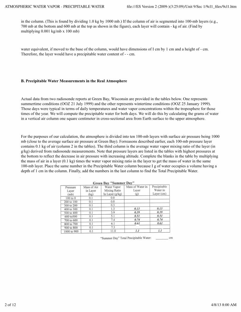
in the column. (This is found by dividing 1.0 kg by 1000 mb.) If the column of air is segmented into 100-mb layers (e.g.,700 mb at the bottom and 600 mb at the top as shown in the figure), each layer will contain - kg of air. (Find bymultiplying 0.001 kg/mb x 100 mb)

water equivalent, if moved to the base of the column, would have dimensions of I cm by 1 cm and a height of - cm.Therefore, the layer would have a precipitable water content of - - cm.

B. Precipitable Water Measurements in the Real Atmosphere

Actual data from two radiosonde reports at Green Bay, Wisconsin are provided in the tables below. One representssummertime conditions (OOZ 21 July 1999) and the other represents wintertime conditions (OOZ 25 January 1999).Those days were typical in terms of daily temperatures and water vapor concentrations within the troposphere for thosetimes of the year. We will compute the precipitable water for both days. We will do this by calculating the grams of waterin a vertical air column one square centimeter in cross-sectional area from Earth surface to the upper atmosphere.

For the purposes of our calculation, the atmosphere is divided into ten 100-mb layers with surface air pressure being 1000mb (close to the average surface air pressure at Green Bay). Forreasons described earlier, each 100-mb pressure layercontains 0.1 kg of air (column 2 in the tables). The third column is the average water vapor mixing ratio of the layer (ing/kg) derived from radiosonde measurements. Note that pressure layers are listed in the tables with highest pressures atthe bottom to reflect the decrease in air pressure with increasing altitude. Complete the blanks in the table by multiplyingthe mass of air in a layer (0.1 kg) times the water vapor mixing ratio in the layer to get the mass of water in the same100-mb layer. Place the same number in the Precipitable Water column because I g of water occupies a volume having adepth of 1 cm in the column. Finally, add the numbers in the last column to find the Total Precipitable Water.


2 of 12 4/8/13 8:00 AM

5. Comparing the total precipitable water amounts for the two days, the atmosphere over Green Bay contained more watervapor in [(summer) (winter)].

6. Both days were similar in that the water vapor concentration [(increased) (did not change) (decreased)] with increasingaltitude. 7. Comparing mixing ratios in the same pressure layers of the lower atmosphere (from 1000 mb to 300 mb) onthe two days, the atmospheric column over Green Bay contained more water vapor in each layer in [(winter) (summer)).

8. The concentration of water vapor in air depends to a large extent on air temperature, with the maximum possibleconcentration increasing with rising temperature. Consequently, higher air temperatures mean more evaporation andhigher concentrations of water vapor in the air.

In general, one would expect [(higher) (lower)] values of precipitable water at polar latitudes where average temperaturesare [(higher) (lower)] than at tropical latitudes where average temperatures are [(higher) (lower)].

9. Many measurements over time indicate that worldwide the atmosphere contains an average of2.5 cm (1.0 in.) ofprecipitable water. Other measurements find that the worldwide average annual precipitation is about 90 cm (35 in.).These measurements indicate that the water vapor in the atmosphere must be completely replaced about 36 times over thecourse of a year to account for 90 cm of precipitation. In other words, the total water vapor in the atmosphere must bereplaced every ________ days. This is the residence time of water in the atmospheric reservoir of the global water budget.

Part 2:


3 of 12 4/8/13 8:00 AM

ATMOSPHERIC WATER VAPOR - PRECIPITABLE WATER

.

In the first part of this investigation, we saw how the amount of water vapor in the atmosphere can be quantified in termsof precipitable water and how values of precipitable water can vary between winter and summer. Significant differencesin precipitable water also occur from one place to another and are associated with the circulation and temperaturedifferences in large-scale weather systems. In this portion of the investigation, we examine some general relationshipsbetween precipitable water values and large-scale weather systems of middle latitudes.

Image 1

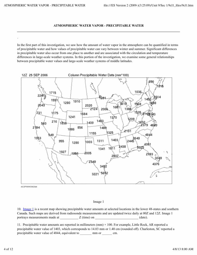
10. Image 1 is a recent map showing precipitable water amounts at selected locations in the lower 48-states and southernCanada. Such maps are derived from radiosonde measurements and are updated twice daily at 00Z and 12Z. Image 1portrays measurements made at ___________ Z (time) on __________________________ (date).

11. Precipitable water amounts are reported in millimeters (mm) × 100. For example, Little Rock, AR reported aprecipitable water value of 1403, which corresponds to 14.03 mm or 1.40 cm (rounded off). Charleston, SC reported aprecipitable water value of 4844, equivalent to _______ mm or ______ cm.


4 of 12 4/8/13 8:00 AM

12. If all the water vapor in the air over Charleston, SC condensed and became rain (and no new water vapor were addedto or removed from the air over Charleston), total rainfall would be _______ cm or ________in. (2.54 cm = 1.0 in.)

13. The highest precipitable water value on the map is [(0.22) (3.49) (5.33)] cm and the lowest value is _____ cm. Circlethese values on your Image 1 map.

14. Precipitable water maps can be analyzed to find patterns of atmospheric water content. On the precipitable watermap, use a pencil to shade all stations reporting values of 2500 (equivalent to 2.5 cm or higher). Also, shade the areasbetween these stations to reveal broad regions of air with relatively high water vapor content. Based on your analysis,precipitable water values are highest over [(the north-central states) (much of the southeast) (the Pacific Northwest)].

Image 2

15. Image 2 is a surface weather map representing conditions at 12Z on 25 SEP 2006, the same time as the precipitablewater values in Image 1. As indicated by the shaded radar echoes (color coded on-screen with intensity scale along theleft margin), a narrow band of rain stretches from South Carolina northeastward to off the southeast coast of NorthCarolina. The rain is occurring in association with a frontal system marking the leading edge of cooler and drier air. Therainfall over the Carolinas [(is) (is not)] consistent with the relatively high precipitable water values in the same regionsas shown in Image 1.

16. Image 2 also shows a broad area of relatively cool air over the Rocky Mountain States. (On the map, temperatures areplotted in ºF at the 11 o'clock position of individual station reports. A sprawling high pressure system ("H") with centers


5 of 12 4/8/13 8:00 AM

of highest pressure in Wyoming and Colorado corresponds to this air mass. This cool air mass swept southward fromCanada over the previous several days. Based on precipitable water reports in Image 1, the air mass associated with thehigh is relatively [(dry) (humid)] compared to the air mass over the southeastern states.

17. Comparing Images 1 and 2, as the cold front (blue line with triangles) moves southeastward across Georgia andFlorida, precipitable water values across southeast Georgia and central Florida should [(decrease) (increase)].

Part 3:

WATER VAPOR IMAGERY

Educational Outcomes: Although water vapor is invisible to our eyes, special sensors aboard weather satellites candetect its presence in the atmosphere. Measurements made by these sensors enable meteorologists to determine thelocation, relative concentration, and movement of water vapor. Water vapor satellite imagery depicts the transport ofwater vapor over thousands of kilometers and to great altitudes as an essential pathway in the global water cycle.

A. Basis of Water Vapor Imagery

Water vapor imagery is a valuable remote sensing tool for tracking the broad scale movement of water vapor within theatmosphere. What is the scientific basis for water vapor imagery?

Just like most other gaseous air molecules, water molecules absorb and emit radiation selectively by wavelength. Satellitesensors that produce conventional infrared (thermal) images detect infrared radiation emitted by the Earth's surface andatmosphere in the so- called atmospheric windows, that is, within wavelength bands from 10.5 to 12.6 micrometers.These wavelengths of infrared radiation are not absorbed or emitted by water vapor. But water vapor and clouds stronglyabsorb and emit infrared radiation having a wavelength of 6. 7 micrometers. This makes it possible for a satellite infraredsensor that is tuned to 6.7 micrometers to detect water vapor in cloud-free areas as well as clouds.

The intensity of radiation reaching the satellite sensor depends on the amount of water vapor with which the radiationinteracts as it wells up from Earth's surface. Infrared radiation emitted by Earth's surface is absorbed by the overlyingwater vapor. In turn, that water vapor emits radiation upward that is absorbed by water vapor at still higher altitudes. Thisprocess of absorption and emission at successively higher altitudes continues as long as significant water vapor remains tointeract with the outgoing radiation. Water vapor imagery detects water vapor in the atmosphere primarily between about3000 and 7000 m (10,000 to 24,000 ft) corresponding to the layer between 700 mb and 400 mb, commonly referred to asthe middle troposphere.

Water vapor imagery portrays water vapor concentration on a gray scale. At one extreme, black indicates the presence oflittle or no water vapor, whereas at the other extreme, milky white signals a relatively high concentration of water vapor.Clouds appear bright white. Dark areas are generally regions of the atmosphere where air is sinking from above where it


6 of 12 4/8/13 8:00 AM

is relatively dry. Dark streaks indicating very low humidity may be associated with jet streams. Milky swirls of humid airseen on satellite imagery often show the cyclonic circulation of low pressure systems prior to the formation of extensivecloudiness.

Sequential water vapor images viewed in rapid succession to detect motion show water vapor transported horizontally ashuge swirling plumes, often originating in the tropics and moving into higher latitudes. A typical water vapor plume isthousands of kilometers long and several hundred kilometers wide. Plumes supply moisture to hurricanes, clusters ofthunderstorms, and winter storms. In spring and summer, such water vapor plumes have been associated withexceptionally heavy rain and flash floods.

B. Comparing Water Vapor Imagery To Other Satellite Imagery

What information does water vapor imagery provide that visible and conventional infrared imagery does not? How do thedifferent kinds of imagery complement each other? To find out, examine the following visible, infrared, and water vaporimages for 1815Z (1:15 PM COT) 9 June 2000 as Figure 1, parts (a) to (c).


7 of 12 4/8/13 8:00 AM

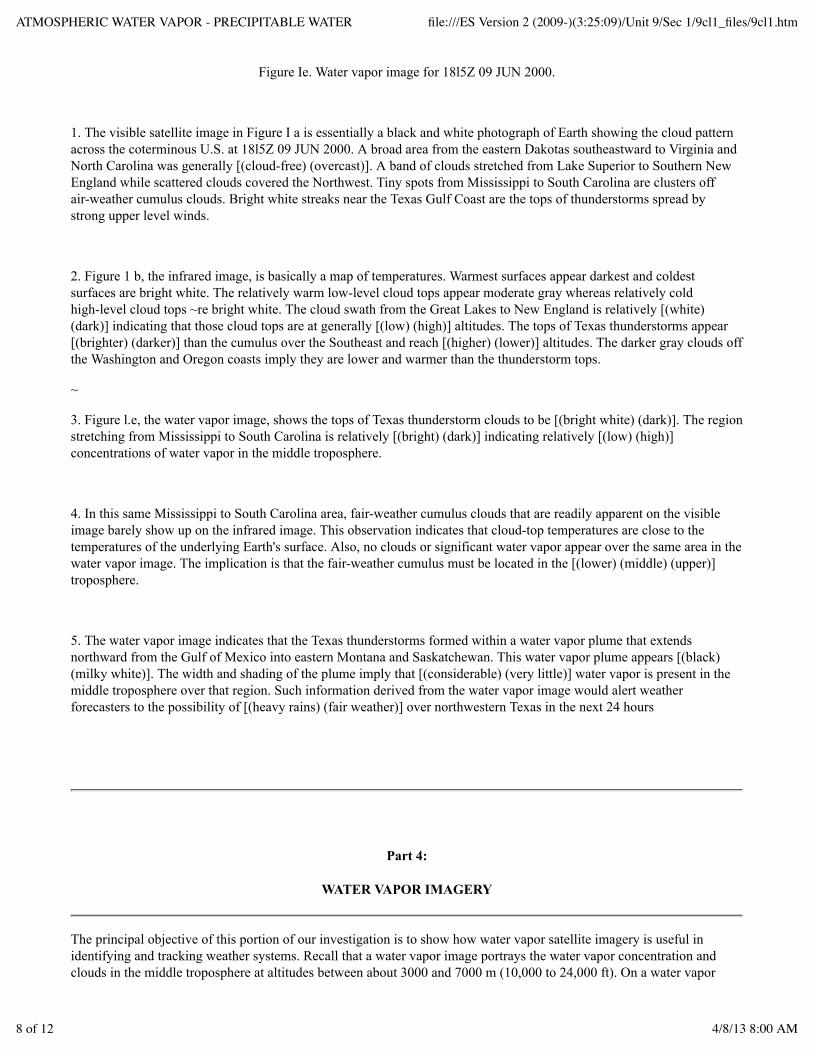
Figure Ie. Water vapor image for 18l5Z 09 JUN 2000.

1. The visible satellite image in Figure I a is essentially a black and white photograph of Earth showing the cloud patternacross the coterminous U.S. at 18l5Z 09 JUN 2000. A broad area from the eastern Dakotas southeastward to Virginia andNorth Carolina was generally [(cloud-free) (overcast)]. A band of clouds stretched from Lake Superior to Southern NewEngland while scattered clouds covered the Northwest. Tiny spots from Mississippi to South Carolina are clusters offair-weather cumulus clouds. Bright white streaks near the Texas Gulf Coast are the tops of thunderstorms spread bystrong upper level winds.

2. Figure 1 b, the infrared image, is basically a map of temperatures. Warmest surfaces appear darkest and coldestsurfaces are bright white. The relatively warm low-level cloud tops appear moderate gray whereas relatively coldhigh-level cloud tops ~re bright white. The cloud swath from the Great Lakes to New England is relatively [(white)(dark)] indicating that those cloud tops are at generally [(low) (high)] altitudes. The tops of Texas thunderstorms appear[(brighter) (darker)] than the cumulus over the Southeast and reach [(higher) (lower)] altitudes. The darker gray clouds offthe Washington and Oregon coasts imply they are lower and warmer than the thunderstorm tops.

~

3. Figure l.e, the water vapor image, shows the tops of Texas thunderstorm clouds to be [(bright white) (dark)]. The regionstretching from Mississippi to South Carolina is relatively [(bright) (dark)] indicating relatively [(low) (high)]concentrations of water vapor in the middle troposphere.

4. In this same Mississippi to South Carolina area, fair-weather cumulus clouds that are readily apparent on the visibleimage barely show up on the infrared image. This observation indicates that cloud-top temperatures are close to thetemperatures of the underlying Earth's surface. Also, no clouds or significant water vapor appear over the same area in thewater vapor image. The implication is that the fair-weather cumulus must be located in the [(lower) (middle) (upper)]troposphere.

5. The water vapor image indicates that the Texas thunderstorms formed within a water vapor plume that extendsnorthward from the Gulf of Mexico into eastern Montana and Saskatchewan. This water vapor plume appears [(black)(milky white)]. The width and shading of the plume imply that [(considerable) (very little)] water vapor is present in themiddle troposphere over that region. Such information derived from the water vapor image would alert weatherforecasters to the possibility of [(heavy rains) (fair weather)] over northwestern Texas in the next 24 hours

Part 4:

WATER VAPOR IMAGERY

The principal objective of this portion of our investigation is to show how water vapor satellite imagery is useful inidentifying and tracking weather systems. Recall that a water vapor image portrays the water vapor concentration andclouds in the middle troposphere at altitudes between about 3000 and 7000 m (10,000 to 24,000 ft). On a water vapor


8 of 12 4/8/13 8:00 AM

satellite image, water vapor appears as milky white, clouds as bright white, and relatively dry air as dark. We compare awater vapor image to atmospheric conditions portrayed on a surface weather map and infrared satellite image at about thesame time. In addition, you will use a special water vapor imagery applet to investigate how changing atmosphericconditions influence what is displayed on a water vapor image.

Image 1

6. Image 1 is the surface weather map for 12Z on 27 September 2006. Shaded areas represent radar echoes caused byprecipitation. Radar is detecting very little precipitation across the nation as fair-weather high pressure systems (H)dominate the weather pattern. A weak low pressure system (L) over the western Great Lakes is producing an area of lightrain. Scattered showers are also occurring in the cool air mass over the northern plains states. Meanwhile a stationaryfront situated offshore of the southeastern states cuts across peninsula Florida and into the Gulf of Mexico.

Note the temperatures at "11 o'clock" and dewpoints at "8 o'clock" (in degrees Fahrenheit) plotted on station models.Miami, FL was reporting a temperature of 79 °F and dewpoint of 71 °F. This is representative of conditions south of thestationary front. Meanwhile, north of the stationary front, Tallahassee, FL had a temperature and dewpoint of 58 and 53°F, respectively. The higher the dewpoint values, the more humid the air. The stationary front separated relatively [(cooland dry) (warm and more humid)] air to the southeast from relatively [(cool and dry) (mild and more humid)] air to thenorth and west as shown by the temperatures and dewpoints reported at individual stations.


9 of 12 4/8/13 8:00 AM

Image 2

7. Image 2 is the satellite water vapor image for 1215 Z on 27 September 2006, about the same time as the surfaceweather map in Image 1. On your water vapor image, use a pencil to outline the areas of precipitation associated with thelow-pressure system over the western Great Lakes and the Dakotas based on the location of the shaded radar patterns onthe surface weather map. Areas of precipitation and the distribution of extensive moisture across the United Statesdepicted on the water vapor image appear to be [(generally related) (not related)].

8. Image 2 also shows a close association between the front situated off the southeast coast and an elongated region of[(cloudiness and moist) (generally dry)] conditions in the mid-troposphere to the south and east of the surface frontallocation. Mid-tropospheric winds at map time across the southeastern U.S. were generally from the southwest.Consequently the water-vapor plume that appears to be supplying moisture to the frontal system was coming from the[(the Pacific Northwest) (the Gulf of Mexico)].

9. On the water vapor Image 2, the area across the southeastern states north and west of the stationary front indicates[(very dry) (very humid)] air in the middle troposphere. The water vapor Image 2 indicates generally [(dry) ( humid)]conditions in the middle troposphere from northern California east-southeastward to Texas. In this region, thecombination of surface dewpoint values (Image 1) and moisture conditions in the middle troposphere would indicaterelatively [(high) (low)] amounts of precipitable water and a(n) [(low) (high)] likelihood of precipitation.


10 of 12 4/8/13 8:00 AM

Image 3

10. Image 3 is the infrared satellite image for the same time as the water vapor Image 2. Comparing the infrared imagewith the concurrent surface weather map (Image 1) indicates that cloudiness, as shown by the bright shadings, is generally[(absent) (extensive)] along the front that is draped across the north central states and [(absent) (extensive)] along thefront offshore of the southeastern states.

11. Comparing the infrared satellite image (Image 3) with the water vapor image (Image 2) indicates that areas of veryhumid air in the middle troposphere generally [(do) (do not)] correspond to areas of extensive cloud cover.

In summary, water vapor imagery reveals flows of water vapor in Earth's atmosphere. These flows are integral to theglobal water cycle and knowledge about them in near real-time provides extremely important information leading to moreaccurate storm and precipitation predictions.

Water Vapor Imagery Applet

In this part of the investigation, you can use a special applet to investigate how cloud altitude and upper atmospherichumidity alter the appearance of water vapor imagery. Go to http://profhorn.aos.wisc.edu/wxwise/watervapor/WaterVaporImagery.htm. This applet was developed by Tom Whittaker and Steve Ackerman of the Department ofAtmospheric and Oceanic Sciences and the Space Science and Engineering Center of the University of Wisconsin-Madison.

The applet allows you to manipulate cloud altitude and upper tropospheric humidity. By doing so, you can observeresulting changes in the appearance of a water vapor image. It's fun. Try it.


11 of 12 4/8/13 8:00 AM


12 of 12 4/8/13 8:00 AM

atmospheric water vapor - precipitable water · unit 9 section 1 lab part 1: atmospheric water...

Documents