atmospheric volatile organic compound measurements...

Atmospheric volatile organic compound measurements during

the Pittsburgh Air Quality Study: Results, interpretation, and

quantification of primary and secondary contributions

Dylan B. Millet,1,2 Neil M. Donahue,3 Spyros N. Pandis,3 Andrea Polidori,4

Charles O. Stanier,2,5 Barbara J. Turpin,4 and Allen H. Goldstein1

Received 3 February 2004; revised 7 April 2004; accepted 22 April 2004; published 25 January 2005.

[1] Primary and secondary contributions to ambient levels of volatile organic compounds(VOCs) and aerosol organic carbon (OC) are determined using measurements at thePittsburgh Air Quality Study (PAQS) during January–February and July–August 2002.Primary emission ratios for gas and aerosol species are defined by correlation withspecies of known origin, and contributions from primary and secondary/biogenic sourcesand from the regional background are then determined. Primary anthropogeniccontributions to ambient levels of acetone, methylethylketone, and acetaldehyde werefound to be 12–23% in winter and 2–10% in summer. Secondary production plusbiogenic emissions accounted for 12–27% of the total mixing ratios for these compoundsin winter and 26–34% in summer, with background concentrations accounting for theremainder. Using the same method, we determined that on average 16% of aerosol OCwas secondary in origin during winter versus 37% during summer. Factor analysis of theVOC and aerosol data is used to define the dominant source types in the region for bothseasons. Local automotive emissions were the strongest contributor to changes inatmospheric VOC concentrations; however, they did not significantly impact the aerosolspecies included in the factor analysis. We conclude that longer-range transport andindustrial emissions were more important sources of aerosol during the study period. TheVOC data are also used to characterize the photochemical state of the atmosphere in theregion. The total measured OH loss rate was dominated by nonmethane hydrocarbonsand CO (76% of the total) in winter and by isoprene, its oxidation products, andoxygenated VOCs (79% of the total) in summer, when production of secondary organicaerosol was highest.

Citation: Millet, D. B., N. M. Donahue, S. N. Pandis, A. Polidori, C. O. Stanier, B. J. Turpin, and A. H. Goldstein (2005),

Atmospheric volatile organic compound measurements during the Pittsburgh Air Quality Study: Results, interpretation, and

quantification of primary and secondary contributions, J. Geophys. Res., 110, D07S07, doi:10.1029/2004JD004601.

1. Introduction

[2] Airborne particulate matter (PM) can adversely affecthuman and ecosystem health, and exerts considerableinfluence on climate. Effective PM control strategies requirean understanding of the processes controlling PM concen-tration and composition in different environments. The

Pittsburgh Air Quality Study (PAQS) is a comprehensive,multidisciplinary project directed at understanding the pro-cesses governing aerosol concentrations in the Pittsburghregion [e.g., Wittig et al., 2004a; Stanier et al., 2004a,2004b]. Specific objectives include characterizing the phys-ical and chemical properties of regional PM, its morphologyand temporal and spatial variability, and quantifying theimpacts of the important sources in the area.[3] Volatile organic compounds (VOCs) can directly

influence aerosol formation and growth via condensationof semivolatile oxidation products onto existing aerosolsurface area [Odum et al., 1996; Jang et al., 2002; Czoschkeet al., 2003], and possibly via the homogeneous nucleationof new particles [Koch et al., 2000; Hoffmann et al., 1998].They also have strong indirect effects on aerosol via theircontrol over ozone production and HOx cycling, which inturn dictate oxidation rates of organic and inorganic aerosolprecursor species. Comprehensive and high time resolutionVOC measurements in conjunction with particle measure-ments thus aid in characterizing chemical conditions con-

JOURNAL OF GEOPHYSICAL RESEARCH, VOL. 110, D07S07, doi:10.1029/2004JD004601, 2005

1Division of Ecosystem Sciences, University of California, Berkeley,California, USA.

2Now at Department of Earth and Planetary Sciences, HarvardUniversity, Cambridge, Massachusetts, USA.

3Department of Chemical Engineering, Carnegie Mellon University,Pittsburgh, Pennsylvania, USA.

4Department of Environmental Sciences, Rutgers University, NewBrunswick, New Jersey, USA.

5Now at Department of Chemical and Biochemical Engineering,University of Iowa, Iowa City, Iowa,USA.

Copyright 2005 by the American Geophysical Union.0148-0227/05/2004JD004601$09.00

D07S07 1 of 17

ducive to particle formation and growth. VOC data can alsoyield information on the nature of source types impactingthe study region [Goldstein and Schade, 2000], photochem-ical aging and transport phenomena [Parrish et al., 1992;McKeen and Liu, 1993], and estimates of regional emissionrates [Barnes et al., 2003; Bakwin et al., 1997], all of whichcan be useful in interpreting other gas and particle phasemeasurements.[4] This paper describes the results from two field deploy-

ments, during January–February 2002 and July–August2002, in which we made in situ VOC measurements along-side the comprehensive aerosol measurements at the PAQSsite, with the aim of specifically addressing the connectionbetween atmospheric trace gases and particle formation andsource attribution. The data set provides an opportunity toexamine aerosol formation and chemistry in the context ofhigh time resolution speciated VOC measurements.[5] The specific goals of this paper include: characteriz-

ing the dominant source types impacting the Pittsburghregion, their composition and variability; assessing therelative importance of different types of VOCs to regionalphotochemistry, and the relationship between aerosol con-centrations and the chemical state of the atmosphere; andquantifying the relative importance of primary and second-ary sources in determining organic aerosol and oxygenatedVOC (OVOC) concentrations. For the latter we quantify theprimary emission ratios for species with multiple sourcetypes, by correlation with combustion and photochemicalmarker compounds.

2. Experimental

2.1. Pittsburgh Air Quality Study (PAQS)

[6] The field component of the Pittsburgh Air QualityStudy was carried out from July 2001 through August 2002.Measurement platforms consisted of a main sampling sitelocated in a park about 6 km east of downtown Pittsburgh,as well as a set of satellite sites in the surrounding region.

For details on the PAQS study, see Wittig et al. [2004a] andthe references cited therein. Measurements described herewere made at the main sampling site.

2.2. VOC Measurements

[7] A schematic of the VOC measurement setup is shownin Figure 1. To provide information on as wide a range ofcompounds as possible, two separate measurement channelswere used, equipped with different preconditioning systems,preconcentration traps, chromatography columns, anddetectors. Channel 1 was designed for preconcentrationand separation of C3–C6 nonmethane hydrocarbons, includ-ing alkanes, alkenes and alkynes, on an Rt-Alumina PLOTcolumn with subsequent detection by FID. Channel 2 wasdesigned for preconcentration and separation of oxygenated,aromatic, and halogenated VOCs, NMHCs larger than C6,and some other VOCs such as acetonitrile and dimethylsul-fide, on a DB-WAX column with subsequent detection byquadropole MSD (HP 5971).[8] Air samples were drawn at 4 sl/min through a

2 micron Teflon particulate filter and 1/400 OD Teflon tubing(FEP fluoropolymer, Chemfluor) mounted on top of thelaboratory container. Two 15 scc/min subsample flows weredrawn from the main sample line, and through pretreatmenttraps for removal of O3, H2O and CO2. For 30 min out ofevery hour, the valve array (V1, V2, and V3; valves fromValco Instruments) was switched to sampling mode(Figure 1, as shown) and the subsamples flowed through0.0300 ID fused silica-lined stainless steel tubing (Silcosteel,Restek Corp) to the sample preconcentration traps wherethe VOCs were trapped prior to analysis. When samplecollection was complete, the preconcentration traps anddownstream tubing were purged with a forward flow ofUHP helium for 30 s to remove residual air. The valve arraywas then switched to inject mode, the preconcentration trapsheated rapidly to 200�C, and the trapped analytes desorbedinto the helium carrier gas and transported to the GC forseparation and quantification.

Figure 1. Schematic of the VOC sampling system. MFC, mass-flow controller; V1–V3, valves 1–3;MSD, mass selective detector; FID, flame ionization detector; PT, pressure transducer.

D07S07 MILLET ET AL.: VOLATILE ORGANICS AT THE PITTSBURGH SUPERSITE

2 of 17

D07S07

[9] As noninert surfaces are known to cause artifacts andcompound losses for unsaturated and oxygenated species,all surfaces contacted by the sampled airstream prior to thevalve array were constructed of Teflon (PFA or FEP). Allsubsequent tubing and fittings, except the internal surfacesof the Valco valves V1, V2, and V3, were Silcosteel. Thevalve array, including all silcosteel tubing, was housed in atemperature controlled box held at 50�C to prevent com-pound losses through condensation and adsorption. Allflows were controlled using Mass-Flo Controllers (MKSInstruments), and pressures were monitored at variouspoints in the sampling apparatus using pressure transducers(Data Instruments).[10] In order to reduce the dew point of the sampled

airstream, both subsample flows passed through a loop of1/800 OD Teflon tubing cooled thermoelectrically to �25�C.Following sample collection, the water trap was heated to105�C while being purged with a reverse flow of dry zeroair to expel the condensed water prior to the next samplinginterval. A trap for the removal of carbon dioxide andozone (Ascarite II, Thomas Scientific) was placed down-stream of the water trap in the Rt-Alumina/FID channel.An ozone trap (KI-impregnated glass wool, followingGreenberg et al. [1994]) was placed upstream of the watertrap in the other channel leading to the DB-WAX columnand the MSD (Figure 1).[11] Sample preconcentration was achieved using a com-

bination of thermoelectric cooling and adsorbent trapping.The preconcentration traps consisted of three stages (glassbeads/Carbopack B/Carboxen 1000 for the Rt-Alumina/FIDchannel, glass beads/Carbopack B/Carbosieves SIII for theDB-WAX/MSD channel; all adsorbents from Supelco), heldin place by DMCS-treated glass wool (Alltech Associates)in a 9 cm long, 0.0400 ID fused silica-lined stainless steeltube (Restek Corp). A nichrome wire heater was wrappedaround the preconcentration traps, and the trap/heaterassemblies were housed in a machined aluminum blockthat was thermoelectrically cooled to �15�C. After samplecollection and the helium purge, the preconcentration trapswere isolated via V3 (see Figure 1) until the start of the nextchromatographic run. The traps were small enough topermit rapid thermal desorption (�15�C to 200�C in 10 s)eliminating the need to cryofocus the samples before chro-matographic analysis (following Lamanna and Goldstein[1999]). The samples were thus introduced to the individualGC columns, where the components were separated andthen detected with the FID or MSD.[12] Chromatographic separation and detection of the

analytes was achieved using an HP 5890 Series II GC.The temperature program for the GC oven was: 35�C for5 min, 3�C/min to 95�C, 12.5�C/min to 195�C, hold for6 min. The oven then ramped down to 35�C in preparationfor the next run. The carrier gas flow into the MSDwas controlled electronically and maintained constant at1 mL/min. The FID channel carrier gas flow was controlledmechanically by setting the pressure at the column headsuch that the flow was 4.5 mL/min at an oven temperatureof 35�C. The carrier gas for both channels was UHP(99.999%) helium which was further purified of oxygen,moisture and hydrocarbons (traps from Restek Corp.).[13] Zero air for blank runs and calibration by standard

addition was generated by flowing ambient air over a bed of

platinum heated to 370�C. This system passes ambienthumidity, creating VOC free air in a matrix resembling realair as closely as possible. Zero air was analyzed daily tocheck for blank problems and contamination for all mea-sured compounds.[14] Compounds measured on the FID channel were

quantified by determining their weighted response relativeto a reference compound (see Goldstein et al. [1995a] andLamanna and Goldstein [1999] for details). Neohexane(5.15 ppm, certified NIST traceable ±2%; Scott-MarrinInc.) was employed as the internal standard for the FIDchannel, and was added by dynamic dilution to the sam-pling stream. Compound identification was achieved bymatching retention times with those of known standardsfor each compound (Scott Specialty Gases, Inc.).[15] The MSD was operated in single ion mode (SIM) for

optimum sensitivity and selectivity of response. Ion-monitoring windows were timed to coincide with the elutionof the compounds of interest. Calibration curves for all ofthe individual compounds were obtained by dynamic dilu-tion of multicomponent low-ppm level standards (Apel-Riemer Environmental Inc.) into zero air to mimic the rangeof ambient mixing ratios. A calibration or blank wasperformed every 6th run.[16] The system was fully automated for unattended

operation in the field. The valve array (V1, V2 and V3)and the preconcentration trap resistance heater circuit werecontrolled through the GC via auxiliary output circuitry. ThePC controlling the GC was also interfaced with a CR10Xdata logger (Campbell Scientific Inc.), which was triggeredat the outset of each analysis run. The inlet valve, thestandard addition solenoid valve and the water trap cooling,heating and valve circuitry were switched at the appropriatetimes during the sampling cycle by a relay module (SDM-CD16AC, Campbell Scientific) controlled by the datalogger. Relevant engineering data (time, temperatures, flowrates, pressures, etc.) for each sampling interval wererecorded by the CR10X data logger with a AM416 multi-plexer (Campbell Scientific Inc.), then uploaded to the PCand stored with the associated chromatographic data. Chro-matogram integrations were done using HP Chemstationsoftware. All subsequent data processing and QA/QCwas performed using routines created in S-Plus (InsightfulCorp.). Instrumental precision, detection limits, andaccuracy for each measured compound during this experi-ment, along with the 0.25, 0.50, and 0.75 quantiles of thedata, are given in Table 1.

2.3. Aerosol, Trace Gas, and MeteorologicalMeasurements

[17] Additional measurements which are used in thispaper are described briefly below. For a more thoroughoverview of the gas and particle measurement methods andresults from PAQS, the reader is directed to Wittig et al.[2004a] and the references cited therein.[18] Semicontinuous measurements of PM 2.5 (i.e.,

<2.5 mm diameter) particulate mass were made using atapering element oscillating microprobe (TEOM) instrument(Model 1400a, Rupprecht & Patashnick Co., Inc.). PM 2.5nitrate and sulfate were also measured on a semicontinuousbasis using Integrated Collection and Vaporization Cell(ICVC) instruments (Rupprecht & Patashnick Co., Inc.)


3 of 17

D07S07

[Wittig et al., 2004b]. Aerosol number size distributions(0.003–10 mm) were quantified using an array of particlesizing measurements: a nano scanning mobility particle sizer(SMPS) (TSI, Inc., Model 3936N25), standard SMPS (TSI,Inc., Model 3936L10), and Aerodynamic Particle Sizer(APS) (TSI, Inc., Model 3320). Aerosol number size distri-bution measurements were made semicontinuously through-out the PAQS campaign [Stanier et al., 2004a]. Aerosolorganic carbon (OC) and elemental carbon (EC) werequantified in situ throughout the study with 2–4 hour timeresolution using a Sunset Labs in situ carbon analyzer(A. Polidori et al., manuscript in preparation, 2005).[19] O3, NO, NO2, CO and SO2 were measured contin-

uously with commercial gas analyzers (Models 400A,

200A, 300 and 100A, Teledyne Advanced Pollution Instru-mentation). Measurements of relevant meteorologicalparameters (incoming radiation, air temperature, wind speedand direction, precipitation, and relative humidity) were alsomade continuously throughout the experiment.

3. Results and Discussion

3.1. Meteorological Conditions

[20] Observed wind speed and direction for the two studyperiods (9 January to 12 February and 9 July to 10 August2002) are shown as a wind rose plot in Figure 2. Through-out this paper, data collected during the January–February2002 deployment will be referred to as ‘‘winter’’ data and

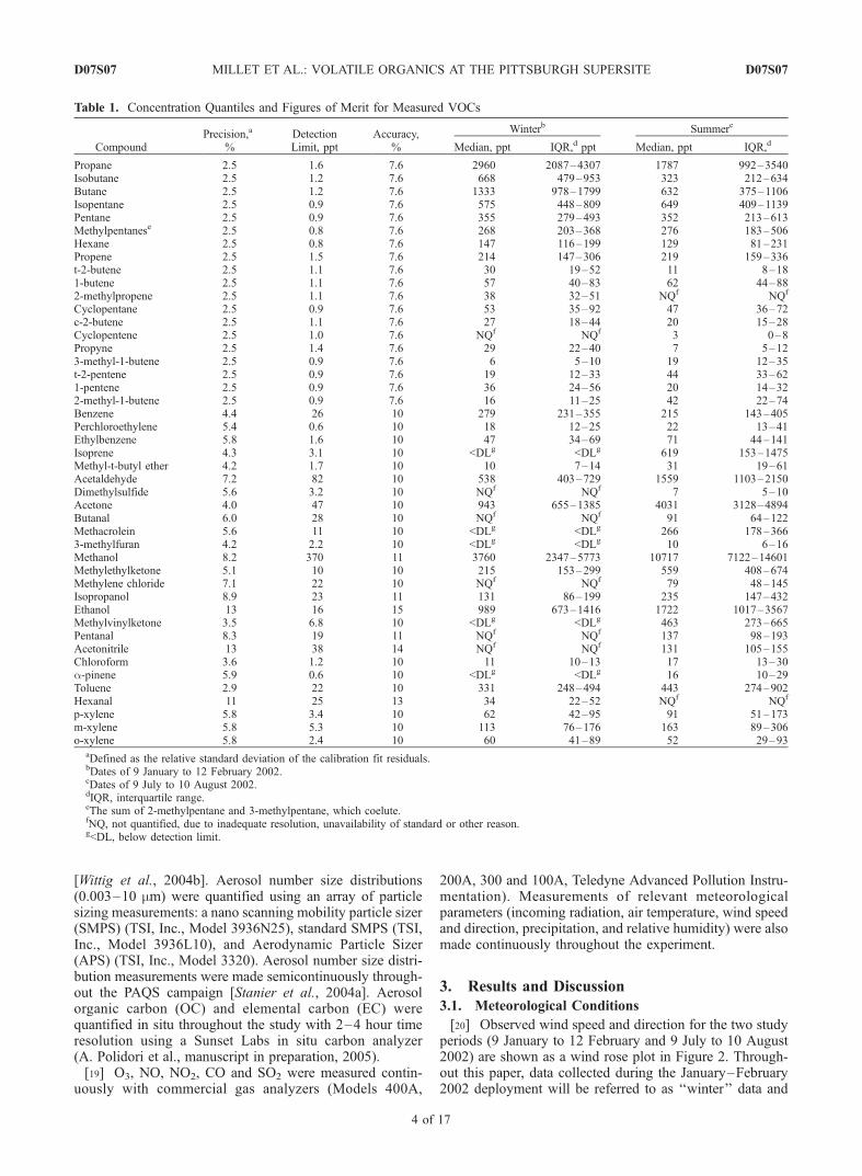
Table 1. Concentration Quantiles and Figures of Merit for Measured VOCs

CompoundPrecision,a

%DetectionLimit, ppt

Accuracy,%

Winterb Summerc

Median, ppt IQR,d ppt Median, ppt IQR,d

Propane 2.5 1.6 7.6 2960 2087–4307 1787 992–3540Isobutane 2.5 1.2 7.6 668 479–953 323 212–634Butane 2.5 1.2 7.6 1333 978–1799 632 375–1106Isopentane 2.5 0.9 7.6 575 448–809 649 409–1139Pentane 2.5 0.9 7.6 355 279–493 352 213–613Methylpentanese 2.5 0.8 7.6 268 203–368 276 183–506Hexane 2.5 0.8 7.6 147 116–199 129 81–231Propene 2.5 1.5 7.6 214 147–306 219 159–336t-2-butene 2.5 1.1 7.6 30 19–52 11 8–181-butene 2.5 1.1 7.6 57 40–83 62 44–882-methylpropene 2.5 1.1 7.6 38 32–51 NQf NQf

Cyclopentane 2.5 0.9 7.6 53 35–92 47 36–72c-2-butene 2.5 1.1 7.6 27 18–44 20 15–28Cyclopentene 2.5 1.0 7.6 NQf NQf 3 0–8Propyne 2.5 1.4 7.6 29 22–40 7 5–123-methyl-1-butene 2.5 0.9 7.6 6 5–10 19 12–35t-2-pentene 2.5 0.9 7.6 19 12–33 44 33–621-pentene 2.5 0.9 7.6 36 24–56 20 14–322-methyl-1-butene 2.5 0.9 7.6 16 11–25 42 22–74Benzene 4.4 26 10 279 231–355 215 143–405Perchloroethylene 5.4 0.6 10 18 12–25 22 13–41Ethylbenzene 5.8 1.6 10 47 34–69 71 44–141Isoprene 4.3 3.1 10 <DLg <DLg 619 153–1475Methyl-t-butyl ether 4.2 1.7 10 10 7–14 31 19–61Acetaldehyde 7.2 82 10 538 403–729 1559 1103–2150Dimethylsulfide 5.6 3.2 10 NQf NQf 7 5–10Acetone 4.0 47 10 943 655–1385 4031 3128–4894Butanal 6.0 28 10 NQf NQf 91 64–122Methacrolein 5.6 11 10 <DLg <DLg 266 178–3663-methylfuran 4.2 2.2 10 <DLg <DLg 10 6–16Methanol 8.2 370 11 3760 2347–5773 10717 7122–14601Methylethylketone 5.1 10 10 215 153–299 559 408–674Methylene chloride 7.1 22 10 NQf NQf 79 48–145Isopropanol 8.9 23 11 131 86–199 235 147–432Ethanol 13 16 15 989 673–1416 1722 1017–3567Methylvinylketone 3.5 6.8 10 <DLg <DLg 463 273–665Pentanal 8.3 19 11 NQf NQf 137 98–193Acetonitrile 13 38 14 NQf NQf 131 105–155Chloroform 3.6 1.2 10 11 10–13 17 13–30a-pinene 5.9 0.6 10 <DLg <DLg 16 10–29Toluene 2.9 22 10 331 248–494 443 274–902Hexanal 11 25 13 34 22–52 NQf NQf

p-xylene 5.8 3.4 10 62 42–95 91 51–173m-xylene 5.8 5.3 10 113 76–176 163 89–306o-xylene 5.8 2.4 10 60 41–89 52 29–93

aDefined as the relative standard deviation of the calibration fit residuals.bDates of 9 January to 12 February 2002.cDates of 9 July to 10 August 2002.dIQR, interquartile range.eThe sum of 2-methylpentane and 3-methylpentane, which coelute.fNQ, not quantified, due to inadequate resolution, unavailability of standard or other reason.g<DL, below detection limit.


4 of 17

D07S07

that collected during July–August 2002 as ‘‘summer’’ data.Winds in the winter were predominantly out of the west(south to northwest), whereas in the summer southeasterlyand northwesterly winds were most common (Figure 2).There was a diurnal cycle in wind speed in both seasons,with stronger winds during the day and weaker winds atnight (not shown).

3.2. Factor Analysis

[21] Factor analysis can be used to categorize measuredcompounds into distinct source groups based on the covari-ance of their concentrations, creating an understanding ofthe variety of sources contributing to a broad range ofmeasured species [Sweet and Vermette, 1992; Thunis andCuvelier, 2000; Lamanna and Goldstein, 1999]. In thissection we characterize the dominant source types impact-ing the Pittsburgh region in summer and winter, based on afactor analysis of the VOC data set, combined with otheravailable trace gas and high temporal resolution aerosoldata. Compounds are grouped into factors according to theircovariance, and the strength of association between com-pounds and factors is expressed as a loading matrix. Eachfactor is a linear combination of the observed variables andin theory represents an underlying process which is causingcertain species to behave similarly. Prior knowledge ofsource types for the dominant compounds is then used toassign source categories to the statistically identified factors.[22] The analysis was performed using principal compo-

nents extraction and varimax rotation (S-Plus 6.1, LucentTechnologies Inc.). Species having a significant amount(>8%) of missing data were excluded from the analysis.Results for the winter and summer data sets are presented inTables 2 and 3, respectively, and discussed in detail below.Compounds not loading significantly on any of the factorsare omitted from the loadings tables.3.2.1. Winter Trace Gas and Aerosol Data Set[23] Six factors were extracted from the winter data set,

which accounted for a total of 83% of the cumulativevariance (Table 2). Each of the six factors accounted for astatistically significant portion of the variance (P < 0.01,where P is the statistical probability of incorrectly attribut-ing a nonzero fraction of the variance to a given factor). Theanalysis was limited to six factors since including morefactors failed to account for more than an additional 2% ofthe variance in the data set.[24] Factor 1, explaining 44% of the total variability in

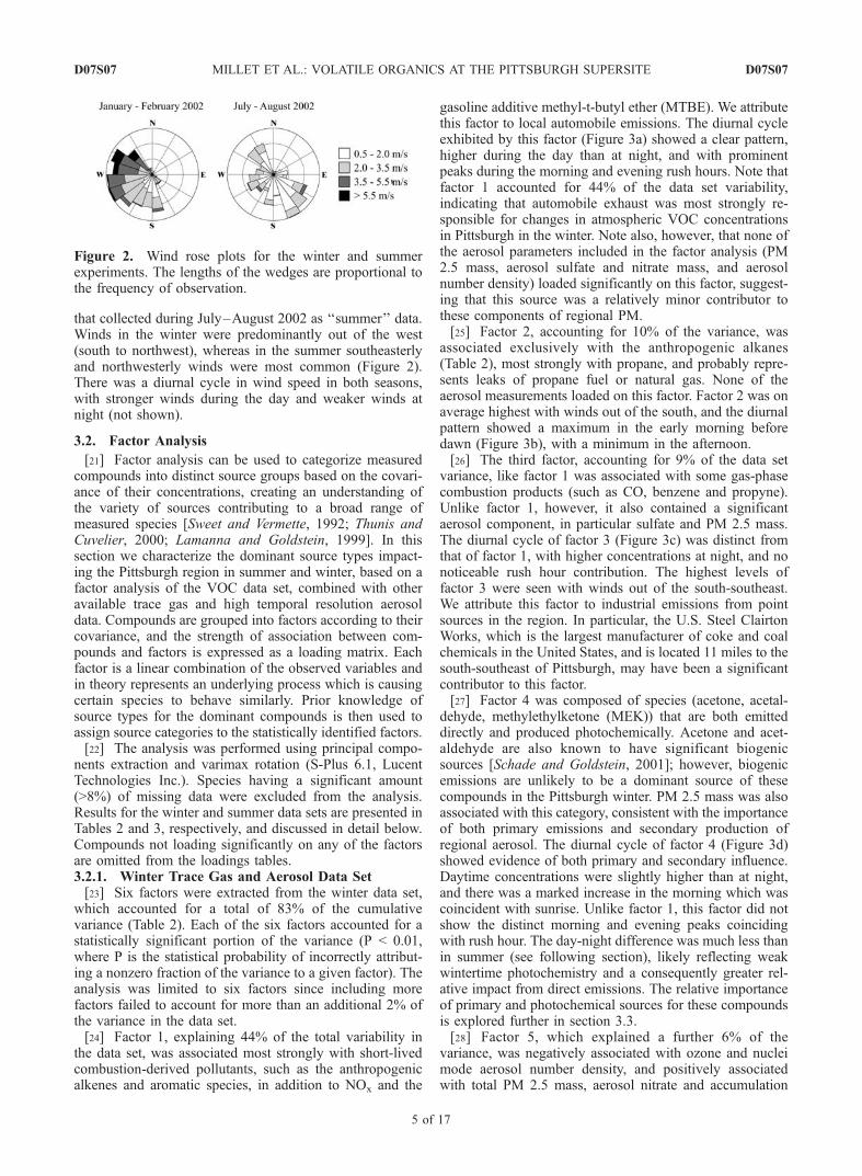
the data set, was associated most strongly with short-livedcombustion-derived pollutants, such as the anthropogenicalkenes and aromatic species, in addition to NOx and the

gasoline additive methyl-t-butyl ether (MTBE). We attributethis factor to local automobile emissions. The diurnal cycleexhibited by this factor (Figure 3a) showed a clear pattern,higher during the day than at night, and with prominentpeaks during the morning and evening rush hours. Note thatfactor 1 accounted for 44% of the data set variability,indicating that automobile exhaust was most strongly re-sponsible for changes in atmospheric VOC concentrationsin Pittsburgh in the winter. Note also, however, that none ofthe aerosol parameters included in the factor analysis (PM2.5 mass, aerosol sulfate and nitrate mass, and aerosolnumber density) loaded significantly on this factor, suggest-ing that this source was a relatively minor contributor tothese components of regional PM.[25] Factor 2, accounting for 10% of the variance, was

associated exclusively with the anthropogenic alkanes(Table 2), most strongly with propane, and probably repre-sents leaks of propane fuel or natural gas. None of theaerosol measurements loaded on this factor. Factor 2 was onaverage highest with winds out of the south, and the diurnalpattern showed a maximum in the early morning beforedawn (Figure 3b), with a minimum in the afternoon.[26] The third factor, accounting for 9% of the data set

variance, like factor 1 was associated with some gas-phasecombustion products (such as CO, benzene and propyne).Unlike factor 1, however, it also contained a significantaerosol component, in particular sulfate and PM 2.5 mass.The diurnal cycle of factor 3 (Figure 3c) was distinct fromthat of factor 1, with higher concentrations at night, and nonoticeable rush hour contribution. The highest levels offactor 3 were seen with winds out of the south-southeast.We attribute this factor to industrial emissions from pointsources in the region. In particular, the U.S. Steel ClairtonWorks, which is the largest manufacturer of coke and coalchemicals in the United States, and is located 11 miles to thesouth-southeast of Pittsburgh, may have been a significantcontributor to this factor.[27] Factor 4 was composed of species (acetone, acetal-

dehyde, methylethylketone (MEK)) that are both emitteddirectly and produced photochemically. Acetone and acet-aldehyde are also known to have significant biogenicsources [Schade and Goldstein, 2001]; however, biogenicemissions are unlikely to be a dominant source of thesecompounds in the Pittsburgh winter. PM 2.5 mass was alsoassociated with this category, consistent with the importanceof both primary emissions and secondary production ofregional aerosol. The diurnal cycle of factor 4 (Figure 3d)showed evidence of both primary and secondary influence.Daytime concentrations were slightly higher than at night,and there was a marked increase in the morning which wascoincident with sunrise. Unlike factor 1, this factor did notshow the distinct morning and evening peaks coincidingwith rush hour. The day-night difference was much less thanin summer (see following section), likely reflecting weakwintertime photochemistry and a consequently greater rel-ative impact from direct emissions. The relative importanceof primary and photochemical sources for these compoundsis explored further in section 3.3.[28] Factor 5, which explained a further 6% of the

variance, was negatively associated with ozone and nucleimode aerosol number density, and positively associatedwith total PM 2.5 mass, aerosol nitrate and accumulation

Figure 2. Wind rose plots for the winter and summerexperiments. The lengths of the wedges are proportional tothe frequency of observation.


5 of 17

D07S07

mode number density. This factor may represent the com-bined influences of photochemical activity and mixed layerdynamics. Production of ozone and nucleation mode par-ticles is driven by sunlight, and owing to their relativelyshort lifetimes their concentrations were highest during theday and lower at night. By contrast, longer lived pollutantsless strongly impacted by photochemistry exhibited higherconcentrations at night when winds were calmer and verti-cal mixing limited. In addition, partitioning of semivolatilespecies such as nitrate into the particle phase is thermody-namically favored by the colder temperatures and higherrelative humidity at night.[29] The 6th factor, accounting for 6% of the variability,

was associated with gas phase SO2, aerosol sulfate, PM 2.5mass, and accumulation mode number density. Factor 6showed a diurnal pattern with higher impact during the daythan at night, consistent with a photochemically driven

process (Figure 3f). However, nucleation mode numberdensity did not load significantly on this factor. This factormay reflect regional coal burning power plant emissions ofgases and particles, and the subsequent photochemicalaging of those emissions.3.2.2. Summer Trace Gas and Aerosol Data Set[30] Six factors were extracted from the summer data set,

which together accounted for 77% of the variability in theobservations (Table 3). Each of the six factors accounted fora statistically significant portion of the variance (P < 0.01).Including additional factors explained less than 2% of theremaining variance. The PM 2.5 measurements had a largenumber (19%) of missing values, and as there was a strongcorrelation (r2 = 0.92) between PM 2.5 mass and aerosolvolume measured with the SMPS, missing PM 2.5 concen-trations were estimated by scaling to aerosol volume prior toperforming the factor analysis.

Table 2. Factor Analysis Results: Winter Dataa

Compound

Loadings

Factor 1:Local Auto

Factor 2:Natural Gas

Factor 3:Industrial

Factor 4:1� + 2�

Factor 5:2� + Mix

Factor 6:Coal

Propane 0.87Isobutane 0.64 0.66Butane 0.63 0.63t-2-butene 0.90Isopentane 0.76 0.49Pentane 0.63 0.62Methylpentanesb 0.77 0.44Hexane 0.65 0.54Propene 0.76 0.471-butene 0.862-methylpropene 0.60 0.49Cyclopentane 0.57c-2-butene 0.91Propyne 0.64 0.533-methyl-1-butene 0.90t-2-pentene 0.901-pentene 0.912-methyl-1-butene 0.91Benzene 0.42 0.63C2Cl4 0.68Ethylbenzene 0.89MTBE 0.74Acetaldehyde 0.41 0.58Acetone 0.82MEK 0.47 0.64Chloroform 0.52Toluene 0.80Hexanal 0.61p-xylene 0.90m-xylene 0.91o-xylene 0.90O3 �0.68NOx 0.76SO2 0.75CO 0.52 0.59PM 2.5 0.50 0.42 0.44 0.40Aerosol SO4

2� 0.54 0.54Aerosol NO3

� 0.62Nnuc

c �0.42Nacc

c 0.41 0.45 0.59Importance of factorsFraction of variance 0.44 0.10 0.09 0.08 0.06 0.06Cumulative variance 0.44 0.54 0.63 0.71 0.77 0.83

aThe degree of association between measured compounds and each of the six factors is indicated by a loading value, with themaximum loading being 1. Loadings of magnitude <0.4 omitted.

bThe sum of 2-methylpentane and 3-methylpentane, which coelute.cNnuc and Nacc refer to aerosol number densities in the nuclei (3–10 nm) and accumulation (100–500 nm) modes.


6 of 17

D07S07

[31] As with the winter data, the dominant factor, explain-ing 42% of the total variance, was associated with anthropo-genic alkenes, aromatics, MTBE and other markers oftailpipe emissions (Table 3). The diurnal cycle of this sourcetype (Figure 4a), however, with a sharp early morningmaximum at sunrise and a broad afternoon minimum, wasmarkedly different than in the winter, when traffic patternsdetermined the diurnal pattern. In summer, a deeper daytimemixed layer and more rapid photooxidation combined to giverise to the observed temporal pattern. The fact that benzene isnot associated with factor 1 is due to the influence of a nearbysource (not associated with other tailpipe compounds orsolvents), which resulted occasionally in extremely elevatedbenzene levels. If the factor analysis is repeated after remov-

ing the highest (>0.9 quantile) benzene values, benzene infact loads most strongly on this automotive factor.[32] Factor 2 encompassed compounds, such as acetone,

acetaldehyde, and isoprene, known to have photochemicalsources, sunlight dependent biogenic sources, or both. Wethus interpret this factor as representing a combination ofthese radiation-driven source types. The clear diurnal pat-tern for this source category (Figure 4b) reflected its lightdependent nature, and suggests, for the associated OVOCs,that photochemical and/or biogenic production were moreimportant than direct combustion emissions. The associa-tion of 1-butene with factor 2 suggests a regional light-driven biogenic 1-butene source, as has been reported forother locations [Goldstein et al., 1996].

Table 3. Factor Analysis Results: Summer Dataa

Compound

Loadings

Factor 1:Local Auto

Factor 2:2� + Bio

Factor 3:Transport

Factor 4:Industrial

Factor 5:Isopentane Ox

Factor 6:Natural Gas

Propane 0.59 0.58Isobutane 0.74 0.54Butane 0.78 0.52Isopentane 0.91Pentane 0.89Methylpentanesb 0.93Hexane 0.90Propene 0.71 0.45t-2-butene 0.891-butene 0.57 0.66Cyclopentane 0.66 0.49c-2-butene 0.80Propyne 0.883-methyl-1-butene 0.95t-2-pentene 0.941-pentene 0.932-methyl-1-butene 0.82Benzene 0.68C2Cl4 0.48Ethylbenzene 0.89Isoprene 0.44MTBE 0.91Acetaldehyde 0.88Acetone 0.64 0.64Butanal 0.85MACR 0.903-methylfuran 0.45 0.53MEK 0.44 0.44 0.40Isopropanol 0.47MVK 0.89Pentanal 0.55 0.72Acetonitrile 0.43Chloroform 0.67a-pinene 0.57Toluene 0.80 0.47p-xylene 0.90m-xylene 0.90o-xylene 0.84O3 �0.51 �0.43NOx 0.52 0.44SO2 0.42CO 0.50 0.44PM 2.5 0.88Aerosol SO4

2� 0.85Nacc

c 0.70Importance of factorsFraction of variance 0.42 0.10 0.08 0.07 0.05 0.04Cumulative variance 0.42 0.53 0.60 0.67 0.73 0.77

aThe degree of association between measured compounds and each of the six factors is indicated by a loading value, with themaximum loading being 1. Loadings of magnitude <0.4 omitted.

bThe sum of 2-methylpentane and 3-methylpentane, which coelute.cAccumulation mode (100–500 nm) aerosol number density.


7 of 17

D07S07

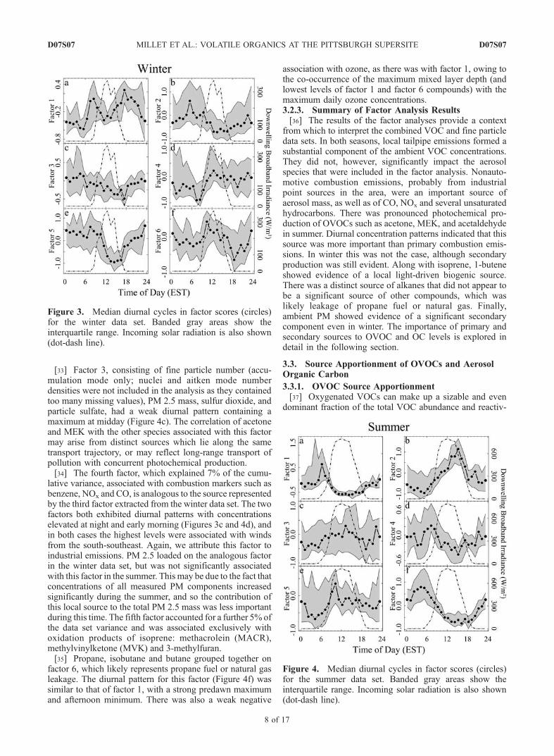
[33] Factor 3, consisting of fine particle number (accu-mulation mode only; nuclei and aitken mode numberdensities were not included in the analysis as they containedtoo many missing values), PM 2.5 mass, sulfur dioxide, andparticle sulfate, had a weak diurnal pattern containing amaximum at midday (Figure 4c). The correlation of acetoneand MEK with the other species associated with this factormay arise from distinct sources which lie along the sametransport trajectory, or may reflect long-range transport ofpollution with concurrent photochemical production.[34] The fourth factor, which explained 7% of the cumu-

lative variance, associated with combustion markers such asbenzene, NOx and CO, is analogous to the source representedby the third factor extracted from the winter data set. The twofactors both exhibited diurnal patterns with concentrationselevated at night and early morning (Figures 3c and 4d), andin both cases the highest levels were associated with windsfrom the south-southeast. Again, we attribute this factor toindustrial emissions. PM 2.5 loaded on the analogous factorin the winter data set, but was not significantly associatedwith this factor in the summer. This may be due to the fact thatconcentrations of all measured PM components increasedsignificantly during the summer, and so the contribution ofthis local source to the total PM 2.5 mass was less importantduring this time. The fifth factor accounted for a further 5% ofthe data set variance and was associated exclusively withoxidation products of isoprene: methacrolein (MACR),methylvinylketone (MVK) and 3-methylfuran.[35] Propane, isobutane and butane grouped together on

factor 6, which likely represents propane fuel or natural gasleakage. The diurnal pattern for this factor (Figure 4f) wassimilar to that of factor 1, with a strong predawn maximumand afternoon minimum. There was also a weak negative

association with ozone, as there was with factor 1, owing tothe co-occurrence of the maximum mixed layer depth (andlowest levels of factor 1 and factor 6 compounds) with themaximum daily ozone concentrations.3.2.3. Summary of Factor Analysis Results[36] The results of the factor analyses provide a context

from which to interpret the combined VOC and fine particledata sets. In both seasons, local tailpipe emissions formed asubstantial component of the ambient VOC concentrations.They did not, however, significantly impact the aerosolspecies that were included in the factor analysis. Nonauto-motive combustion emissions, probably from industrialpoint sources in the area, were an important source ofaerosol mass, as well as of CO, NOx and several unsaturatedhydrocarbons. There was pronounced photochemical pro-duction of OVOCs such as acetone, MEK, and acetaldehydein summer. Diurnal concentration patterns indicated that thissource was more important than primary combustion emis-sions. In winter this was not the case, although secondaryproduction was still evident. Along with isoprene, 1-buteneshowed evidence of a local light-driven biogenic source.There was a distinct source of alkanes that did not appear tobe a significant source of other compounds, which waslikely leakage of propane fuel or natural gas. Finally,ambient PM showed evidence of a significant secondarycomponent even in winter. The importance of primary andsecondary sources to OVOC and OC levels is explored indetail in the following section.

3.3. Source Apportionment of OVOCs and AerosolOrganic Carbon

3.3.1. OVOC Source Apportionment[37] Oxygenated VOCs can make up a sizable and even

dominant fraction of the total VOC abundance and reactiv-

Figure 3. Median diurnal cycles in factor scores (circles)for the winter data set. Banded gray areas show theinterquartile range. Incoming solar radiation is also shown(dot-dash line).

Figure 4. Median diurnal cycles in factor scores (circles)for the summer data set. Banded gray areas show theinterquartile range. Incoming solar radiation is also shown(dot-dash line).


8 of 17

D07S07

ity, in the urban [Grosjean, 1982; Goldan et al., 1995a],rural [Goldan et al., 1995b; Riemer et al., 1998], and evenremote marine atmosphere [Singh et al., 1995, 2001]. ManyOVOCs, such as acetone, MEK and acetaldehyde, areknown to have a diversity of sources, including combustionemissions, photochemical production from both anthropo-genic and biogenic precursor species, and direct biogenicemissions. Understanding the magnitudes of these sourcesin different environments is prerequisite to an accuraterepresentation of odd hydrogen cycling and ozone chemis-try in models of atmospheric chemistry and air quality fromthe local to global scale.[38] Here we present a new approach to unraveling source

contributions to such species. We define the ambient con-centrations of VOC species Y (cy, in ppt) as being the sumof direct combustion (cyc) and other components (cyo),which could represent secondary or biogenic sources, aswell as a background concentration (ca),

cy ¼ cyc þ cyo þ ca: ð1Þ

[39] For relatively long lived species, such as acetone, ca

may be considered to represent a regional background level.In this case, ca will presumably include contributions fromboth combustion and secondary/biogenic production thathas taken place elsewhere and been integrated into theregional background. For acetaldehyde, a compound withan atmospheric lifetime of only a few hours, there wasnonetheless a nonzero observed minimum concentration inboth summer and winter. Here, the parameter ca mayrepresent a relatively invariant area source that maintainsambient levels of acetaldehyde above a certain threshold. Ineither case, we operationally define the background con-centration of each species as the 0.1 quantile of themeasured concentrations [Goldstein et al., 1995b].[40] If Y and a combustion tracer, such as toluene, are

emitted in a relatively consistent ratio from different typesof combustion sources, then cyc can be estimated as

cyc ¼ ctol

Y

TOL

� �E

; ð2Þ

where (Y/TOL)E is the primary emission ratio of Y relativeto toluene, and ctol represents toluene enhancements abovebackground (ppt; see the following section for a discussionof the choice of combustion marker). cyo is then given by

cyo ¼ cy � ctol

Y

TOL

� �E

� ca: ð3Þ

In (3), ctol, cy, and ca are known quantities. All that isrequired to calculate the combustion (cyc) and secondaryplus biogenic (cyo) components of species Y is the primaryemission ration (Y/TOL)E.[41] To determine (Y/TOL)E for each species Y, we make

use of the combustion tracers associated with the first factorin the factor analyses (Tables 2 and 3). For a given value of(Y/TOL)E, we can calculate a cyo vector, and the coefficientof determination (r2) between cyo and each of our combus-tion tracers. By varying (Y/TOL)E over a range of possiblevalues and repeating this calculation, we can derive r2

between the calculated cyo and each of our combustiontracers, as a function of (Y/TOL)E. At low values of (Y/TOL)E,the calculated cyo will still contain a significant combustioncomponent. At high values of (Y/TOL)E, cyo will becomedominated by thectol term. At the correct value for (Y/TOL)Eall contributions of combustion emissions should be removedfrom cyo, and hence correlation of cyo with a pure combus-tion parameter should be at a minimum. Conversely, if thenoncombustion sources of Y are dominantly photochemical,then the correlation between cyo and a photochemicallyderived VOC should reach a maximum at that same point.[42] The results of performing this analysis for Y =

acetone, MEK and acetaldehyde are shown in Figure 5.Each solid line shows the coefficient of determinationbetween an individual combustion marker and cyo, as afunction of the value of (Y/TOL)E that was used to calculatecyo. The compounds used as markers of combustion(V, with mixing ratios cv) were those VOCs thought to

Figure 5. Coefficient of determination between combus-tion or photochemically derived VOCs and the residual termcyo, representing photochemical and biogenic OVOCsources, as a function of the primary emission ratio(Y/TOL)E. Each solid (dashed) line represents a separatecombustion (photochemical) marker compound (V, withmixing ratio cv, for V = propyne, 2-methylpropene,t-2-butene, c-2-butene, 2-methyl-1-butene, 3-methyl-1-butene, t-2-pentene, benzene, ethylbenzene, p-xylene,m-xylene, o-xylene, NOx, MACR, or MVK). The criticalpoint in the curves gives the combustion emission ratio forspeciesY (acetone,MEK,or acetaldehyde) relative to toluene.


9 of 17

D07S07

be solely or predominantly derived via combustion pro-cesses (propyne, 2-methylpropene, t-2-butene, c-2-butene,2-methyl-1-butene, 3-methyl-1-butene, t-2-pentene,benzene, ethylbenzene, p-xylene, m-xylene, o-xylene) andNOx. Dashed lines show r2 between cyo and VOCs thoughtto be solely photochemically produced (MACR and MVK,which were present above detection limit in the summerexperiment only), as a function of (Y/TOL)E.[43] There is a well defined minimum in the curve for the

combustion markers, the location of which, for a givenoxygenated VOC species Y, is consistent across all markercompounds. For the summer data, the location of thisminimum coincides with the maximum r2 value for thephotochemically produced tracer species. We interpret thelocation of the critical value of r2 as the representative (Y/TOL)E value for that time of year (Table 4).[44] Primary emission ratios, relative to toluene, for

acetone, MEK and acetaldehyde were all substantially(1.4–2.4 times) higher in January–February 2002 than inJuly–August 2002. Since the emission ratio depends on thetoluene as well as OVOC emission strength, seasonalchanges in the emission ratio can be due to changes in thenumerator, denominator or both. This issue is discussedfurther in the following section. The primary emission ratioscalculated in this section are averages over the sourcesimpacting the air masses that were sampled during thecourse of the study. They therefore represent integratedregional emission ratios for Pittsburgh in January–Februaryand July–August 2002.[45] Urban and industrial VOC emission ratios depend on

a number of factors, in particular vehicle fleet and fuelcharacteristics as well as types of industrial activity in theregion. Such variability complicates efforts to constructreliable emission inventories for use in air quality modeling,and emphasizes the utility of the approach developed here,which provides top-down observational constraints onregional pollutant emission ratios. On-road studies of motorvehicle exhaust in the U.S. (generally carried out duringsummer) report emission ratios for acetone, MEK andacetaldehyde relative to toluene ranging from 2–4%, 2–12%, and <1–8% (molar basis) respectively for light-dutyvehicles [Kirchstetter et al., 1999; Fraser et al., 1998;Zielinska et al., 1996; Kirchstetter et al., 1996]. Heavy-dutyor diesel vehicles emit substantially higher amounts of theseOVOCs relative to toluene, with emission ratios frequently

greater than unity [Zielinska et al., 1996; Staehelin et al.,1998]. Inventory estimates (including mobile, point andnonpoint sources) of annual acetaldehyde and MEK emis-sions in Allegheny County are 14% and 10% those oftoluene respectively on a molar basis (see http://www.epa.gov/ttn/chief/net/index.html), substantially lower than thevalues determined here (Table 4). If inventory estimates oftoluene emissions are accurate, this suggests that acetalde-hyde and MEK emissions are underestimated by factors ofapproximately 3.8 and 2.6 (from the average of the summerand winter ratios, Table 4).[46] For the summer data, cyo for both acetone and MEK

exhibited a well-defined maximum correlation with MACRand MVK (Figure 5), indicating that the other, noncombus-tive, source represented by cyo is likely to be largelyphotochemical. For acetaldehyde, the poor correlation ofcyo with MACR and MVK suggests that cyo is notexclusively photochemical in nature, and may containanother significant component such as biogenic emissions.[47] For comparison, Figure 6 shows results of the same

analysis for Y = MACR and MVK, species whose onlysignificant known source is from photochemical oxidationof isoprene. In this case, the minimum correlation of cyo

with combustion derived VOCs (and maximum correlationwith MVK or MACR) occurs at a combustion emissionratio (Y/TOL)E of zero, showing that there are no significantprimary emissions of these compounds.[48] With (Y/TOL)E determined by the critical points in

Figure 5, the contributions to the concentration of species Yfrom background (ca), combustion emissions (cyc), andother sources (cyo) as a function of time can then becalculated from (2) and (3). Contributions of ca, cyc, andcyo to the ambient levels of acetone, MEK, and acetalde-hyde in summer and winter are summarized in Table 4.Negative values of cyo were assumed to contain no sec-ondary or biogenic material and were set to zero.[49] Ambient concentrations of acetone, MEK and acet-

aldehyde during summer were on average 3–4 times higherthan winter (Table 4). Increases in background concentra-tions were responsible for a significant portion of this winterto summer difference, with summer background levels onaverage 2.5–5 times higher than in the winter. However, thefraction of the total concentration due to the backgroundwas comparable in summer and winter. In both seasons, thebackground made up, on average, slightly over half of the

Table 4. OVOC Combustion Emission Ratios and Source Contributionsa

Species (Y)

AmbientConcentration

Primary EmissionRatio

BackgroundConcentration Combustion Emissions Other Sources

cy, ppt (Y/TOL)E ca,ppt

ca/cy cyc, ppt cyc/cy cyo, ppt cyo/cy

Median IQRb Median IQRb Median IQRb Median IQRb Median IQRb Median IQRb Median IQRb

WinterAcetone 943 655–1390 0.78 0.74–0.82 526 0.56 0.38–0.80 114 49–241 0.12 0.05–0.21 237 23–624 0.24 0.04–0.48MEK 215 153–299 0.34 0.34–0.34 120 0.56 0.40–0.79 50 21–105 0.23 0.10–0.39 24 0–92 0.12 0.00–0.35Acetaldehyde 538 403–729 0.62 0.60–0.64 289 0.54 0.40–0.72 91 39–192 0.17 0.07–0.31 146 24–290 0.27 0.05–0.40

SummerAcetone 4030 3130–4890 0.32 0.29–0.34 2650 0.66 0.54–0.85 81 29–224 0.02 0.01–0.06 1200 353–1940 0.29 0.12–0.41MEK 559 408–674 0.17 0.16–0.18 319 0.57 0.47–0.78 45 16–123 0.10 0.03–0.23 138 29–257 0.26 0.06–0.40Acetaldehyde 1560 1100–2150 0.43 0.40–0.52 798 0.51 0.37–0.72 113 40–310 0.09 0.03–0.20 542 126–1050 0.34 0.11–0.50

aNote that the median values of the source contributions do not necessarily add up to the median ambient concentration as the median is not a distributiveproperty.

bIQR, interquartile range.


10 of 17

D07S07

overall abundance for all three compounds (Table 4). Thehigher summer background concentrations for these specieswere probably due to increased nonlocal photochemicalproduction and biogenic emission during that time of year.[50] The absolute contribution from combustion to atmo-

spheric mixing ratios was very similar in summer andwinter, despite the large changes in emission ratios (whichwere higher in winter by factors of 2.4, 2.0 and 1.4 foracetone, MEK and acetaldehyde; see discussion in follow-ing section). However, total concentrations were substan-

tially higher in summer, and combustion emissions were asignificantly smaller fraction of the total source (Table 4).[51] Other sources, which we assume to be predominantly

photochemical but which also likely include some biogenicemissions in summer, were substantially higher in summerfor all three compounds. Median summer values of cyo

were over 5 times higher than in winter for acetone andMEK and nearly 4 times higher for acetaldehyde.[52] With the exception of MEK, combustion was not the

major source of these compounds, even in winter. For MEK,combustion emissions were more important than othersources (cyo) in the winter (a median of 23% versus13%). This was not the case in the summer, however, norwas it true for acetone or acetaldehyde in either season. Foracetone, other sources were twice as important as combus-tion emissions in the winter and ten times as important inthe summer. For acetaldehyde, other sources were 50%larger than combustion emissions in winter and 4 timeslarger in summer.[53] Diurnally averaged OVOC source contributions,

overlaid with ozone concentrations, in winter and summerare shown in Figure 7. For the summer data set, the otherOVOC sources (cyo) showed a strong photochemical sig-nature: low at night, increasing after sunrise and peaking inthe afternoon. For each compound, acetone, MEK andacetaldehyde, the cyo term tracked ozone quite closely.For the winter data set, the cyo terms for each OVOCshowed a much weaker photochemical signal, and therelative contribution from combustion was substantiallylarger than in the summer. Note that since cyc for each

Figure 6. Same as Figure 5, except for Y = methacrolein(MACR) and methylvinylketone (MVK). The minimumcorrelation of cyo with combustion derived VOCs (andmaximum correlation with photochemical VOCs) occurs atan emission ratio (Y/TOL)E of zero, showing that there areno significant primary emissions of these compounds.

Figure 7. Diurnal patterns in OVOC source contributions (winter and summer data). Combustionsource (cyc, ppb), pluses and unshaded region; photochemical and biogenic sources (cyo, ppb), circlesand surrounding gray area. Ozone is also shown (solid dark line). Points show median values; bandedareas show the interquartile range. Note different y axis scales for winter and summer.


11 of 17

D07S07

OVOC is defined as ctol(Y/TOL)E, i.e. the observed tolueneenhancements multiplied by a primary emission ratio,diurnal patterns in cyc shown in Figure 7 reflect that oftoluene.3.3.2. Choice of Combustion Marker and SeasonalPatterns in Emission Ratios[54] Repeating the above analysis using other combustion

derived compounds instead of toluene as the primaryemission tracer resulted in only minor changes to thecalculated OVOC partitioning (Table 4) and did not alterany of the conclusions. This gives us confidence that thisapproach to partitioning VOC source contributions isrobust. For a given primary emission tracer, the calculatedOVOC emission ratios, given by the critical r2, wereconsistent using compounds that are solely combustionderived (e.g. alkenes and alkynes) and compounds thathave additional anthropogenic noncombustion sources, suchas evaporative losses and chemical processing (e.g. benzeneand toluene). Hence the approach is not sensitive to slightdifferences in source profiles for the marker compounds. Weconclude that the calculated emission ratios represent anintegrated regional primary pollution signal, rather than onespecific source type.[55] In addition, we note that the combustion markers

employed to calculate the OVOC primary emission ratiosrelative to toluene (Figure 5) have lifetimes that vary bynearly a factor of 50, yet they give consistent emission ratioestimates. This may indicate that much of the variabilityobserved is relatively local and not driven by photochemicallifetime or by the different sampling footprints for species ofdifferent lifetimes.[56] Seasonal differences in the OVOC primary emission

ratios, however, calculated relative to the tracer compound,changed dramatically depending on the tracer used. This isto be expected since the primary emission ratios aresensitive to changes in both the numerator and denominator,and different combustion tracers do not necessarily haveidentical seasonal patterns in emission strength. While theprimary OVOC emission ratios relative to toluene were allhigher in the winter, OVOC emission ratios calculatedrelative to alkenes and alkynes were generally 2–3 timeshigher in the summer. It is possible that noncombustiontoluene sources, i.e. evaporative emissions, are higher insummer which would decrease the OVOC emission ratio forthat time of year. However, the short-lived alkenes areoxidized much more rapidly in the summer months due tohigher concentrations of OH and ozone. Over a givensource-receptor distance, then, the alkenes would be moredepleted relative to the OVOCs in the summer than in thewinter. This would lead to higher OVOC:alkene emissionratios in the summer, as observed. While this effect wouldalso occur with toluene, either the effect was small due totoluene’s longer lifetime (10 times that of t-2-butene) and/orit was offset by increased emissions.3.3.3. Quantification of Secondary Organic Aerosol[57] Organic carbon (OC) constitutes a significant frac-

tion of atmospheric aerosol [Lim and Turpin, 2002; Cabadaet al., 2002, 2004; Tolocka et al., 2001]; however, its originand composition remain poorly understood. OC consists ofhundreds or thousands of individual organic compounds.Both anthropogenic sources (e.g. combustion) and biogenicsources (e.g. plants) can contribute to aerosol organic

carbon via direct emission of particles (primary OC), andvia emission of gas-phase precursor compounds that parti-tion into the aerosol phase upon oxidation (secondary OC).Clarifying the roles of primary and secondary OC produc-tion is an important step toward an improved understandingand modeling of the sources, morphology and effects ofaerosol OC. The technique of minimizing (maximizing) thecorrelation between combustion (photochemical) tracercompounds and the photochemical component of a speciesof interest, developed in the previous section, also has utilityin determining the primary emission ratio for pollutantsother than VOCs. Here, we apply the method to quantify therelative importance of primary and secondary OC sources inthe study region.[58] As above, aerosol organic carbon concentrations

(Moc, in mg of carbon per cubic meter, mgC/m3) are definedas being composed of combustion (Mc) and other (Mo)components, plus a regional background (Ma) [Turpin andHuntzicker, 1995]:

Moc ¼ Mc þMo þMa: ð4Þ

[59] Elemental carbon (EC, or soot) is an aerosol com-ponent whose only source is direct emission from combus-tion. If both OC and EC are emitted from primary sourcesaccording to a characteristic averaged OC:EC emission ratio(OC/EC)E, then the combustion-derived organic carbon canbe estimated as

Mc ¼ Mec

OC

EC

� �E

; ð5Þ

where Mec represents elemental carbon enhancements abovebackground (in mgC/m3), and Mo is given by

Mo ¼ Moc �Mec

OC

EC

� �E

� Ma: ð6Þ

[60] The background term, Ma, represents noncombustionprimary OC (e.g. from biogenic sources) as well as anyregional aerosol organic carbon background. As above, weestimate Ma as the 0.1 quantile of the measured OCconcentrations. Mo is then assumed to be exclusivelysecondary OC. It should be pointed out, however, that ifthere exist significant sources of primary OC which do notcorrelate with EC and are highly variable through time (andthus are not entirely captured by the Ma parameter), then Mo

may also contain some primary influence.[61] One challenge associated with the EC tracer method

as it has been applied in the past involves defining theOC:EC ratio of primary emissions, as this can vary signif-icantly between sources and consequently as a function oftime. In addition, defining (OC/EC)E from ambient OC andEC concentration data requires that there be a subset of datawith no significant secondary contributions to the measuredOC concentrations. The typical approach is to qualitativelyeliminate data points that are likely to be impacted bysignificant secondary production or other factors such asrain events, and regress OC on EC for that subset of datadominated by primary OC [Turpin and Huntzicker, 1995;Cabada et al., 2004]. This then gives a regression slope thatis in theory reflective solely of primary emissions. The


12 of 17

D07S07

parameterMa, reflecting primary noncombustion OC, is thenassumed to be constant and given by the intercept, enablingthe calculation of Mo. In the event of significant temporalvariability in the primaryOC:EC ratio impacting the samplingsite, this process may be repeated on subsets of the data.[62] Here we employ the technique developed in the

previous section, using the range of markers for primaryand secondary processes provided by the VOC data set todefine the characteristicOC:ECprimary emission ratio for thePittsburgh region in summer and winter. This approachavoids the need to carefully select time periods that will yieldthe ‘‘correct’’ value of (OC/EC)E. In addition, the suite ofprimary and secondary VOCs available provides bounds onthe value of (OC/EC)E appropriate to a given time period. Thesecondary organic aerosol is then calculated according to (6).[63] The coefficient of determination between Mo and

combustion and photochemically derived VOCs is shown inFigure 8 as a function of (OC/EC)E for winter and summer.Again, the critical point of the curves gives the representa-tive value of (OC/EC)E for that time of year.[64] The median value of (OC/EC)E determined for the

winter data set was 1.85 (IQR: 1.82–1.86), whereas that forthe summer data set was lower with a median of 1.36 (IQR:1.27–1.48) (Table 5). Substantially higher particulate con-centrations of levoglucosan were observed in the winter,indicative of increased wood combustion. More widespreadwood burning is a likely cause of the higher primary OC:ECemission ratio at that time of year. Colder engines and lessefficient combustion may have also contributed to thehigher wintertime ratio.

[65] Using the derived values of (OC/EC)E for summerand winter, we can then calculate Mo, the secondary OC,according to (6). Timelines of the total (Moc), combustion(Mc), and secondary (Mo) aerosol organic carbon concen-trations (in mgC/m3) for winter and summer 2002 are plottedin Figure 9, and quantiles of these quantities are given inTable 5. Note that since Mc is defined as Mec(OC/EC)E,there are occasional episodes where Mc > Moc. Negativevalues of Mo were assumed to contain no secondarymaterial and were set to zero.[66] Ambient concentrations of aerosol organic carbon in

the summer experiment were on average twice as high as inthe winter (Table 5). Background levels (Ma) made up asignificant fraction of the total ambient aerosol OC concen-trations in both seasons. Background aerosol OC concen-trations were slightly higher in summer but a larger fractionof the total in winter (median of 49% versus 35%).Similarly, combustion OC was slightly higher in the sum-mer, however, it made up a larger fraction of the total OC inwinter (median of 30% versus 19%). Secondary organiccarbon (Mo) accounted for a median of 16% (IQR: 0–35%)of the aerosol OC in winter, and 37% (IQR: 15–56%) insummer (Table 5).[67] A. Polidori et al. (manuscript in preparation, 2005)

carried out an analysis of the primary and secondarycomponents of OC in Pittsburgh during the PAQS study

Figure 8. Coefficient of determination between combus-tion or photochemically derived VOCs and the residual termMo, representing secondary OC, as a function of the primaryemission ratio (OC/EC)E. Each solid (dashed) line repre-sents a separate combustion (photochemical) markercompound. The critical point in the curves gives theprimary emission ratio (OC/EC)E.

Table 5. OC Combustion Emission Ratios and Source Contributionsa

Season

AmbientConcentration

PrimaryEmissionRatio

BackgroundConcentration Combustion Emissions Secondary Production

Moc,mgC/m3 (OC/EC)E Ma,

mgC/m3

Ma/Moc

Mc,mgC/m3 Mc/Moc

Mo,mgC/m3 Mo/Moc

Median IQRb Median IQRb Median IQRb Median IQRb Median IQRb Median IQRb Median IQRb

Winter 1.2 0.83–2.0 1.85 1.82–1.86 0.60 0.49 0.30–0.72 0.37 0.13–0.75 0.30 0.13–0.48 0.20 0.00–0.59 0.16 0.00–0.35Summer 2.5 1.6–3.9 1.36 1.27–1.48 0.87 0.35 0.22–0.54 0.50 0.20–1.1 0.19 0.10–0.32 0.99 0.27–1.9 0.37 0.15–0.56

aNote that the median values of the source contributions do not necessarily add up to the median ambient concentration as the median is not a distributiveproperty.

bIQR, interquartile range.

Figure 9. Timelines of total OC (Moc, mgC/m3), dark solid

line; combustion OC (Mc, mgC/m3), dashed line; secondary

OC (Mo, mgC/m3), light solid line. Data are shown for the

(a) winter and (b) summer deployments.


13 of 17

D07S07

using the Turpin and Huntzicker [1995] EC tracer method.For overlapping time periods (10 January to 12 Februaryand 10–31 July 2002), they calculate median secondaryOC concentrations of 0.21 mgC/m3 (15% of total OC) and1.04 mgC/m3 (47% of total OC) respectively. Thesevalues are in good agreement with those calculated herefor the same periods: 0.20 mgC/m3 (16% of total OC) and1.15 mgC/m3 (43% of total OC) (note that these values differslightly from those in Table 5 since they do not reflectidentical time periods).

3.4. Characterization of the Chemical State of theAtmosphere: VOC Contributions to OH Loss

[68] Photochemical production of secondary organicaerosol (SOA) depends on the chemical state of the atmo-sphere, both in terms of oxidative capacity, and in term ofthe quantity and nature of gas phase organic material that ispresent to form aerosol. In this section we describe therelative importance of different classes of VOCs to tropo-spheric photochemistry in the Pittsburgh region in summerand winter, and show that higher levels of photochemicallyactive compounds are present in summer, when SOA levelsare highest, due to biogenic emissions and photochemicalproduction of OVOCs.[69] A useful measure of air mass chemical reactivity is

the OH loss rate (LOH, s�1), defined as

LOH ¼Xi

kici; ð7Þ

where ki is the reaction rate constant for species i with thehydroxyl radical [Atkinson, 1994], and ci is the concentra-tion of i in molec/cm3. LOH has units of s�1 and representsthe inverse lifetime of the hydroxyl radical with respect toreaction with the measured compounds.[70] Daytime (1000–1600 EST) values of LOH were

calculated for the following groups of compounds: total(all measured VOCs plus CO); alkanes; alkenes + alkynes;aromatics; OVOCs; isoprene plus its oxidation productsmethacrolein, methylvinylketone, and 3-methylfuran; andCO (Figure 10; Tables 6 and 7).[71] Due to analytical challenges, VOC measurements in

many field studies of air quality and atmospheric chemistrycomprise only the anthropogenic nonmethane hydrocarbons(NMHCs; alkanes, alkenes, alkynes and aromatics). InPittsburgh during January and February 2002, these speciesaccounted for a substantial portion (approximately 60%) ofthe total measured OH loss rate. However, while theircollective OH reactivity was only slightly less in summer(0.68 s�1 versus 0.89 s�1), their importance relative to otherVOCs was dramatically lower, as they accounted for only11% on average of total LOH during summer. Similarly, theCO reactivity was comparable in both seasons (median of0.49 s�1 in winter and 0.53 s�1 in summer), but its relativecontribution to the total measured OH loss rate was muchgreater in winter (median of 23% versus 7% in the summer).It should be pointed out that these calculations do notinclude the C2 hydrocarbons ethane, ethene and ethyne,which were not measured. Based on published ratios ofthese compounds to other species [Parrish et al., 1998], weestimate that they would cause an OH loss rate of approx-imately 0.05 s�1 and 0.13 s�1 for summer and winter.

[72] Despite the comparable NMHC and CO reactivity inthe two seasons, the total measured daytime OH loss rateunderwent a more than fourfold increase from winter(median = 1.42 s�1; IQR: 1.12–2.30 s�1) to summer(median = 7.25 s�1; IQR: 4.60–9.38 s�1). This was dueto the presence of high levels of isoprene and its oxidationproducts in summer, and also to the three-fold increase inoxygenated VOC concentration and reactivity from winterto summer (Tables 6, 7). Isoprene plus its oxidation prod-ucts accounted for a median of 62% (IQR: 52–70%) of thedaytime OH loss rate in summer, with the OVOCs account-ing for an additional 20% (IQR: 15–26%). Formaldehydemeasurements were not made during the PAQS study, andincluding the effects of this compound would result in anincreased contribution to the calculated OH loss rate fromthe OVOCs in both seasons.[73] The PAQS sampling site was located at the north end

of Schenley Park, a 456 acre urban park with substantialtree cover. To test whether the observed isoprene concen-trations were biased by the presence of a large nearbysource, the daytime OH loss due to isoprene and its

Figure 10. Probability density curves of measured day-time (1000–1600 EST) VOC OH loss rate by compoundclass for winter and summer 2002. Measured OH loss ratefor isoprene plus its oxidation products methacrolein,methylvinylketone, and 3-methylfuran is shown for bothhot (maximum air temperature � 29�C) and cool (maximumair temperature < 29�C) days in the summer. Thesecompounds were not present above detection limit in thewinter. Note the different scales for the x axes in the left-and right-hand columns.


14 of 17

D07S07

oxidation products was calculated for time periods when thewind was only from the northern sector and the wind speedwas greater than 1 m/s. The resulting OH loss rate (median4.55 s�1; IQR 2.85–5.73 s�1) was not significantly differ-ent from that calculated using all of the daytime data

(median 4.71 s�1; IQR 2.77–6.20 s�1). Hence we find thatin winter, the total daytime OH loss rate is dominated by thenonmethane hydrocarbons and CO, whereas in summer it isdominated by isoprene, its oxidation products, and oxygen-ated VOCs. The above calculations do not include methane,

Table 6. Quantiles of Daytime OH Loss Rate: Winter Dataa,b

Category

All Days High Ozone Daysc

LOH, s�1

Fraction of Total VOCLOH LOH, s

�1Fraction of Total VOC

LOH

Median IQRe Median IQRe Median IQRe Median IQRe

Total 1.42 1.12–2.30 1.00 0.91–1.27Alkanesf 0.31 0.25–0.41 0.20 0.17–0.25 0.27 0.17–0.32 0.20 0.18–0.26Alkenes + Alkynesf 0.41 0.32–0.57 0.27 0.23–0.32 0.29 0.23–0.40 0.25 0.22–0.30Aromatics 0.17 0.12–0.23 0.11 0.09–0.13 0.12 0.09–0.19 0.10 0.09–0.12OVOCs 0.41 0.33–0.57 0.29 0.23–0.35 0.45 0.31–0.54 0.38 0.29–0.45CO 0.49 0.21–1.05 0.23 0.17–0.36 0.19 0.19–0.19 0.20 0.20–0.22

Category

High OC Daysc Nucleation Daysd

LOH, s�1



LOH


Total 2.70 1.64–3.35 1.04 0.98–1.20Alkanesf 0.40 0.33–0.58 0.18 0.14–0.20 0.26 0.24–0.30 0.27 0.21–0.29Alkenes + alkynesf 0.57 0.44–0.84 0.24 0.20–0.30 0.28 0.26–0.35 0.28 0.25–0.31Aromatics 0.25 0.14–0.31 0.09 0.07–0.11 0.12 0.10–0.16 0.11 0.09–0.13OVOCs 0.69 0.51–0.78 0.26 0.21–0.32 0.37 0.34–0.45 0.35 0.32–0.38CO 0.74 0.45–1.56 0.28 0.16–0.36 <DLg <DLg <DLg <DLg

aNote that the median values of the components do not necessarily add up to the median of the total as the median is not a distributive property.bDaytime: 1000–1600 EST.cHigh ozone and high OC days are defined as days when the daily maximum concentration was above the 0.8 quantile for all daily maxima.dDays on which moderate to strong nucleation events occurred [Stanier et al., 2004b].eIQR, interquartile range.fNote that ethane, ethene, and ethyne were not measured. See text for discussion.gCO concentrations during these periods were below the instrumental detection limit of 0.1 ppm.

Table 7. Quantiles of Daytime OH Loss Rate: Summer Dataa,b

Category

All Days High Ozone Daysc

LOH, s�1



LOH


Total 7.25 4.60–9.38 8.53 7.17–9.77Alkanesf 0.17 0.12–0.24 0.03 0.02–0.04 0.19 0.17–0.30 0.03 0.02–0.04Alkenes + alkynesf 0.36 0.30–0.45 0.06 0.04–0.07 0.42 0.36–0.51 0.05 0.04–0.06Aromatics 0.14 0.08–0.24 0.02 0.01–0.04 0.13 0.08–0.24 0.02 0.01–0.03OVOCs 1.35 1.09–1.64 0.20 0.15–0.26 1.80 1.53–1.97 0.21 0.16–0.24Isop + Oxf 4.71 2.77–6.20 0.62 0.52–0.70 5.69 3.75–6.67 0.63 0.58–0.71CO 0.53 0.26–0.86 0.07 0.04–0.12 0.60 0.24–0.83 0.06 0.03–0.09

Category

High OC Daysc Nucleation Daysd

LOH, s�1



LOH


Total 9.26 8.23–10.43 4.96 3.37–6.47Alkanesf 0.21 0.16–0.27 0.03 0.02–0.04 0.11 0.09–0.20 0.03 0.02–0.03Alkenes + alkynesf 0.38 0.31–0.48 0.04 0.04–0.06 0.35 0.25–0.43 0.07 0.06–0.07Aromatics 0.27 0.19–0.40 0.03 0.02–0.05 0.12 0.08–0.14 0.02 0.02–0.03OVOCs 1.54 1.35–1.84 0.17 0.14–0.20 1.30 1.05–1.59 0.26 0.23–0.30Isop + Oxg 5.71 4.58–6.75 0.64 0.57–0.70 3.16 1.91–3.92 0.59 0.52–0.62CO 0.71 0.57–1.04 0.09 0.07–0.11 0.22 0.16–0.54 0.07 0.02–0.09

aNote that the median values of the components do not necessarily add up to the median of the total as the median is not a distributive property.bDaytime: 1000–1600 EST.cHigh ozone and high OC days are defined as days when the daily maximum concentration was above the 0.8 quantile for all daily maxima.dDays on which moderate to strong nucleation events occurred [Stanier et al., 2004b].eIQR, interquartile range.fNote that ethane, ethene, and ethyne were not measured. See text for discussion.gIsoprene plus its oxidation products MACR, MVK, and 3-methylfuran.


15 of 17

D07S07

which was not measured during the experiment. Based onbackground concentrations of methane at this latitude (seehttp://www.cmdl.noaa.gov/info/ftpdata.html), we estimatethe OH loss rate in Pittsburgh due to methane at approxi-mately 0.21 s�1 during the winter and 0.32 s�1 during thesummer.[74] Daytime OH loss rates were also calculated on the

following subsets of the data: high ozone days, high aerosolOC days, and days in which moderate to strong nucleationevents were observed [Stanier et al., 2004b] (Tables 6and 7). High ozone and high OC days were defined as daysin which the maximum value of these quantities was abovethe 0.8 quantile for all observed daily maxima.[75] For July and August, the 0.8 concentration quantile

for the daily maximum ozone was 84 ppb. On high ozonedays, the total measured OH loss rate was higher (median:8.53 s�1) than otherwise (days not exceeding this thresholdhad a median OH loss rate of 6.74 s�1), and this increasewas distributed relatively evenly among the different com-pound classes (Table 7). During January and February, the0.8 quantile for daily ozone maxima was only 30 ppb. Daysduring which ozone exceeded this amount had a loweroverall OH loss rate (median 1.00 s�1) than days on whichit did not (median 1.57 s�1). These higher ozone days in thewinter may have occurred during periods of enhancedvertical mixing. Comrie and Yarnal [1992] analyzed thedependence of surface ozone in Pittsburgh on synopticclimatology. They concluded that high ozone levels insummer developed under stagnant anticyclonic conditions,whereas in winter high ozone concentrations were associ-ated with tropopause folding and vertical transport ofstratospheric ozone.[76] In both seasons, days with high OC loadings were

associated with higher levels of all VOC compound cate-gories and CO. In January–February, the median OH lossrate was 2.70 s�1 on days with high OC versus 1.28 s�1 ondays without. In July–August, the median daytime OH lossrate was 9.26 s�1 on high OC days and 6.81 s�1 on otherdays. By contrast, days on which nucleation events occurredhad lower overall OH loss rates (medians of 1.04 s�1 and4.96 s�1 in winter and summer, respectively) than dayswithout nucleation events (medians of 1.54 s�1 and 7.93 s�1

in winter and summer). Stanier et al. [2004b] found that theoccurrence of nucleation events during PAQS was depen-dent on the preexisting aerosol surface area available forcondensation. The lower OH loss rates on nucleation daysmay be due to a positive correlation between gas phasereactivity and aerosol surface area (r2 = 0.48 in winter and0.28 in summer); i.e. less polluted days with low OH lossrates also had lower particle surface area available forcondensation of semivolatile aerosol precursors, whichincreased the likelihood of new particle nucleation.

4. Conclusions

[77] High temporal density speciated VOC measurementsprovide a useful framework for interpreting aerosol mea-surements. Statistical analyses such as factor analysis oncombined VOC-aerosol data sets can test precepts used insource-receptor modeling. The range of combustion andphotochemical markers in the VOC data set also enables usto deconvolve the relative contributions to ambient levels of

OVOCs and aerosol OC from different source types. Wecalculate that secondary plus biogenic sources accounted for24%, 12% and 27% of the ambient concentrations ofacetone, MEK and acetaldehyde respectively in the winterand 29%, 26% and 34% respectively in the summer.Aerosol OC was found to be composed of 16% secondarycarbon in the winter and 37% secondary carbon in thesummer. The importance of the background contribution toobserved concentrations of both OVOCs and aerosol OCemphasizes the role of longer-range transport and the needfor a regional perspective in addressing air quality concerns.While local automotive emissions were the primary factordriving changes in VOC concentrations in Pittsburgh,they did not contribute significantly to variability in theaerosol species included in the factor analysis (PM 2.5mass, aerosol sulfate and nitrate mass, and aerosol numberdensity).[78] VOC concentration data can also help define chem-

ical conditions that are conducive to particle formation andgrowth. We find that while aerosol OC loadings are highestwhen VOC concentrations and reactivities are high, nucle-ation events tended to occur on days when levels of VOCsand CO were low. High ozone days in the summer wereassociated with high OH loss rates due to the VOCs andCO, whereas in the winter the highest ozone levels occurredon days with low levels of CO and nonmethane hydro-carbons but slightly higher OVOC concentrations.[79] One of the overall objectives of the PAQS study is to

develop the ability to predict changes in PM characteristicsand atmospheric composition due to proposed changes inemissions. Reaching this objective will require accuratemodeling of the chemical and dynamical processes control-ling atmospheric composition in the Pittsburgh region. Theresults presented here should help to provide a basis uponwhich to test mechanisms included in such models.

[80] Acknowledgments. This research was conducted as part of thePittsburgh Air Quality Study, which was supported by the US EPA undercontract R82806101 and the US DOE National Energy TechnologyLaboratory under contract DE-FC26-01NT41017. DBM thanks the DOEfor a GREF fellowship. The authors thank all of the PAQS researchers fortheir help; in particular, Allen Robinson, Beth Wittig, and Andrey Khlystov.Thanks also to Megan McKay for her considerable help.

ReferencesAtkinson, R. (1994), Gas phase tropospheric chemistry of organic com-pounds, J. Phys. Chem. Ref. Data Monogr., 2, 1–216.

Bakwin, P. S., D. F. Hurst, P. P. Tans, and J. W. Elkins (1997), Anthropo-genic sources of halocarbons, sulfur hexafluoride, carbon monoxide, andmethane in the southeastern United States, J. Geophys. Res., 102(D13),15,915–15,925.

Barnes, D. H., S. C. Wofsy, B. P. Fehlau, E. W. Gottlieb, J. W. Elkins, G. S.Dutton, and S. A. Montzka (2003), Urban/industrial pollution for theNew York City–Washington, D. C., corridor, 1996–1998: 1. Providingindependent verification of CO and PCE emissions inventories, J. Geo-phys. Res., 108(D6), 4185, doi:10.1029/2001JD001116.

Cabada, J. C., S. N. Pandis, and A. L. Robinson (2002), Sources of atmo-spheric carbonaceous particulate matter in Pittsburgh, Pennsylvania, J. AirWaste Manage., 52(6), 732–741.

Cabada, J. C., S. Takahama, A. Khlystov, S. N. Pandis, S. Rees, C. I.Davidson, and A. L. Robinson (2004), Mass size distributions and sizeresolved chemical composition of fine particulate matter at the PittsburghSupersite, Atmos. Environ., 38(20), 3127–3141.

Comrie, A. C., and B. Yarnal (1992), Relationships between synoptic-scale atmospheric circulation and ozone concentrations in metropolitanPittsburgh, Pennsylvania, Atmos. Environ., 26(3), 301–312.

Czoschke, N. M., M. Jang, and R. M. Kamens (2003), Effect of acidic seedon biogenic secondary organic aerosol growth, Atmos. Environ., 37(30),4287–4299.


16 of 17

D07S07

Fraser, M. P., G. R. Cass, and B. R. T. Simoneit (1998), Gas-phase andparticle-phase organic compounds emitted from motor vehicle trafficin a Los Angeles roadway tunnel, Environ. Sci. Technol., 32(14),2051–2060.

Goldan, P. D., M. Trainer, W. C. Kuster, D. D. Parrish, J. Carpenter, J. M.Roberts, J. E. Yee, and F. C. Fehsenfeld (1995a), Measurements ofhydrocarbons, oxygenated hydrocarbons, carbon monoxide, and nitrogenoxides in an urban basin in Colorado: Implications for emission inven-tories, J. Geophys. Res., 100(D11), 22,771–22,783.

Goldan, P. D., W. C. Kuster, F. C. Fehsenfeld, and S. A. Montzka (1995b),Hydrocarbon measurements in the southeastern United States: The RuralOxidants in the Southern Environment (ROSE) program 1990, J. Geo-phys. Res., 100(D12), 25,945–25,963.

Goldstein, A. H., and G. W. Schade (2000), Quantifying biogenic andanthropogenic contributions to acetone mixing ratios in a rural environ-ment, Atmos. Environ., 34(29–30), 4997–5006.

Goldstein, A. H., B. C. Daube, J. W. Munger, and S. C. Wofsy (1995a),Automated in-situ monitoring of atmospheric non-methane hydrocarbonconcentrations and gradients, J. Atmos. Chem., 21(1), 43–59.

Goldstein, A. H., S. C. Wofsy, and C. M. Spivakovsky (1995b), Seasonalvariations of nonmethane hydrocarbons in rural New England: Con-straints on OH concentrations in northern midlatitudes, J. Geophys.Res., 100(D10), 21,023–21,033.

Goldstein, A. H., S. M. Fan, M. L. Goulden, J. W. Munger, and S. C. Wofsy(1996), Emissions of ethene, propene, and 1-butene by a midlatitudeforest, J. Geophys. Res., 101(D4), 9149–9157.

Greenberg, J. P., B. Lee, D. Helmig, and P. R. Zimmerman (1994), Fullyautomated gas chromatograph-flame ionization detector system for the insitu determination of atmospheric nonmethane hydrocarbons at low partsper trillion concentration, J. Chromatogr. A, 676(2), 389–398.

Grosjean, D. (1982), Formaldehyde and other carbonyls in Los Angelesambient air, Environ. Sci. Technol., 16(5), 254–262.

Hoffmann, T., R. Bandur, U. Marggraf, and M. Linscheid (1998), Molecu-lar composition of organic aerosols formed in the alpha-pinene/O3

reaction: Implications for new particle formation processes, J. Geophys.Res., 103(D19), 25,569–25,578.

Jang, M. S., N. M. Czoschke, S. Lee, and R. M. Kamens (2002), Hetero-geneous atmospheric aerosol production by acid-catalyzed particle-phasereactions, Science, 298(5594), 814–817.

Kirchstetter, T. W., B. C. Singer, R. A. Harley, G. B. Kendall, and W. Chan(1996), Impact of oxygenated gasoline use on California light-dutyvehicle emissions, Environ. Sci. Technol., 30(2), 661–670.

Kirchstetter, T. W., B. C. Singer, R. A. Harley, G. R. Kendall, and J. M.Hesson (1999), Impact of California reformulated gasoline on motorvehicle emissions. 2. Volatile organic compound speciation and reactivity,Environ. Sci. Technol., 33(2), 329–336.

Koch, S., R. Winterhalter, E. Uherek, A. Kolloff, P. Neeb, and G. K.Moortgat (2000), Formation of new particles in the gas-phase ozonolysisof monoterpenes, Atmos. Environ., 34(23), 4031–4042.

Lamanna, M. S., and A. H. Goldstein (1999), In situ measurements of C2–C10 volatile organic compounds above a Sierra Nevada ponderosa pineplantation, J. Geophys. Res., 104(D17), 21,247–21,262.

Lim, H. J., and B. J. Turpin (2002), Origins of primary and secondaryorganic aerosol in Atlanta: Results of time-resolved measurements duringthe Atlanta Supersite experiment, Environ. Sci. Technol., 36(21), 4489–4496.

McKeen, S. A., and S. C. Liu (1993), Hydrocarbon ratios and photochem-ical history of air masses, Geophys. Res. Lett., 20(21), 2363–2366.

Odum, J. R., T. Hoffmann, F. Bowman, D. Collins, R. C. Flagan, and J. H.Seinfeld (1996), Gas/particle partitioning and secondary organic aerosolyields, Environ. Sci. Technol., 30(8), 2580–2585.

Parrish, D. D., C. J. Hahn, E. J. Williams, R. B. Norton, F. C. Fehsenfeld,H. B. Singh, J. D. Shetter, B. W. Gandrud, and B. A. Ridley (1992),Indications of photochemical histories of Pacific air masses from mea-surements of atmospheric trace species at Point Arena, California,J. Geophys. Res., 97(D14), 15,883–15,901.

Parrish, D. D., et al. (1998), Internal consistency tests for evaluation ofmeasurements of anthropogenic hydrocarbons in the troposphere, J. Geo-phys. Res., 103(D17), 22,339–22,359.

Riemer, D., et al. (1998), Observations of nonmethane hydrocarbons andoxygenated volatile organic compounds at a rural site in the southeasternUnited States, J. Geophys. Res., 103(D21), 28,111–28,128.

Schade, G. W., and A. H. Goldstein (2001), Fluxes of oxygenated volatileorganic compounds from a ponderosa pine plantation, J. Geophys. Res.,106(D3), 3111–3123.

Singh, H. B., M. Kanakidou, P. J. Crutzen, and D. J. Jacob (1995), Highconcentrations and photochemical fate of oxygenated hydrocarbons in theglobal troposphere, Nature, 378(6552), 50–54.

Singh, H., Y. Chen, A. Staudt, D. Jacob, D. Blake, B. Heikes, and J. Snow(2001), Evidence from the Pacific troposphere for large global sources ofoxygenated organic compounds, Nature, 410(6832), 1078–1081.

Staehelin, J., C. Keller, W. Stahel, K. Schlapfer, and S. Wunderli (1998),Emission factors from road traffic from a tunnel study (Gubrist tunnel,Switzerland). part III: Results of organic compounds, SO2 and speciationof organic exhaust emission, Atmos. Environ., 32(6), 999–1009.

Stanier, C. O., A. Y. Khlystov, and S. N. Pandis (2004a), Ambient aerosolsize distributions and number concentrations measured during the Pitts-burgh Air Quality Study (PAQS), Atmos. Environ., 38(20), 3275–3284.

Stanier, C. O., A. Y. Khlystov, and S. N. Pandis (2004b), Nucleation eventsduring the Pittsburgh Air Quality Study: Description and relation to keymeteorological, gas phase, and aerosol parameters, Aerosol Sci. Technol.,38(21), 253–264.

Sweet, C. W., and S. J. Vermette (1992), Toxic volatile organic compoundsin urban air in Illinois, Environ. Sci. Technol., 26(1), 165–173.

Thunis, P., and C. Cuvelier (2000), Impact of biogenic emissions on ozoneformation in the Mediterranean area—A BEMA modelling study, Atmos.Environ., 34(3), 467–481.

Tolocka, M. P., P. A. Solomon, W. Mitchell, G. A. Norris, D. B. Gemmill,R. W. Wiener, R. W. Vanderpool, J. B. Homolya, and J. Rice (2001), Eastversus west in the US: Chemical characteristics of PM2.5 during thewinter of 1999, Aerosol Sci. Technol., 34(1), 88–96.

Turpin, B. J., and J. J. Huntzicker (1995), Identification of secondaryorganic aerosol episodes and quantitation of primary and secondaryorganic aerosol concentrations during SCAQS, Atmos. Environ.,29(23), 3527–3544.

Wittig, B., N. Anderson, A. Y. Khlystov, S. N. Pandis, C. Davidson, andA. L. Robinson (2004a), Pittsburgh Air Quality Study overview andinitial scientific findings, Atmos. Environ., 38(20), 3107–3125.

Wittig, B., S. Takahama, A. Khlystov, S. N. Pandis, S. Hering, B. Kirby,and C. Davidson (2004b), Semicontinuous PM2.5 inorganic compositionmeasurements during the Pittsburgh Air Quality Study, Atmos. Environ.,38(20), 3201–3213.

Zielinska, B., J. C. Sagebiel, G. Harshfield, A. W. Gertler, and W. R.Pierson (1996), Volatile organic compounds up to C20 emitted frommotor vehicles: Measurement methods, Atmos. Environ., 30(12),2269–2286.

��A. H. Goldstein, Department of ESPM-Ecosystem Sciences, University

of California, Berkeley, 151 Hilgard Hall, Berkeley, CA 94720, USA.([email protected])N. M. Donahue and S. N. Pandis, Department of Chemical Engineering,

Carnegie Mellon University, 5000 Forbes Ave, Pittsburgh, PA 15213, USA.D. B. Millet, Department of Earth and Planetary Sciences, Harvard

University, Pierce Hall, 29 Oxford St., Cambridge, MA 02138, USA.([email protected])A. Polidori and B. J. Turpin, Department of Environmental Sciences,

Rutgers University, 14 College Farm Rd., New Brunswick, NJ 08901,USA.C. O. Stanier, Department of Chemical and Biochemical Engineering,

University of Iowa, 4122 Seamens Center, Iowa City, IA 52242, USA.


17 of 17

D07S07

atmospheric volatile organic compound measurements...

Documents