atmospheric visibility measurement by a modulated cw lidar

Atmospheric visibility measurement by

a modulated cw lidar

Dennis K. Kreid

A modulated cw lidar is described for the remote sensing of atmospheric visibility. An analysis of the system

response is given, optimum design parameters are established, and the theoretical capabilities of the new

technique are compared with the results of previous work with similar systems. In the new technique, the

output from a low power, cw laser is amplitude-modulated and transmitted by a telescope into the atmo-

sphere where scattering and absorption occur. Backscattered light from along the visible beam path is col-

lected and focused on a detector whose output is filtered and fed into a phase discriminator. The phase of

the return signal (relative to the source) is directly related to the visibility, wherein lies the basis of this tech-

nique.

1. Introduction

Atmospheric visibility or meteorological range isdefined as the distance at which a standardized targetcan just be discerned by a standard observer (i.e., the

distance at which a minimum contrast ratio is achievedas compared to the daytime sky). In free space, the

visibility is essentially infinite, whereas in the atmo-sphere the visual range is reduced due to the extinction

of light by scattering and absorption. Molecular con-stituents contribute to light extinction; however, scat-tering due to the aerosols is normally the dominantextinction process in the atmosphere.

There are numerous practical situations where reli-able measurements of visibility are required: for theconvenience and safety of travelers; for meteorologicalmonitoring and research; and in various industrial sit-uations. Yet most techniques currently employed formeasuring visibility are compromised by limited range,

reliability, and versatility. Consequently, there is agenuine need for the development of alternative meansfor measuring visibility. The goal of the present workis therefore to provide an analysis and evaluation of anew cw lidar technique which has been suggested' forthe measurement of atmospheric visibility. The anal-ysis and experimental results of previous work1 2 on the

new technique are discussed, and a better interpretation

of the results is suggested. Finally, the results of thepresent analysis are utilized to define a prototype ap-

When this work was done the author was with U.S. National Center

for Atmospheric Research; he is now with Battelle Memorial Institute,

Pacific Northwest Laboratories, Richland, Washington 99352.Received 21 November 1975.

paratus for measuring visibility which has several ap-parent advantages when compared to instrumentationthat is currently available.

II. Background

The simplest and most direct approach for measuringatmospheric light extinction (and thereby the visibility)is the double-ended technique consisting of a trans-mitter and receiver separated by a relatively large dis-tance. Although transmissometer systems of this typeare currently widely employed, the double-ended natureof these instruments often precludes their use in certainsituations where visibility information is required.Problems inherent in the double-ended approach in-clude the inconvenience in transporting the instrument,its limited operating range (which depends on thepathlength), and the inability to measure visibility alongpaths above the horizontal.

There is much to be gained by going to a single-endedapproach for measuring visibility. One such approachis the integrating nephelometer3 '4 in which the totalscattering cross section of a sample of aerosol laden gasis estimated from a measurement of the light scatteredby the sample into a solid angle from about 8° to 170°.For homogeneous urban aerosols at relative humiditiesof less than 70%, such measurements have been found5' 6

to be well correlated with visual range. However, ef-fects of the spatial variability of aerosol density andcomposition cannot be detected from a single pointmeasurement. In addition, there are instances wherethe inability to measure the scattering in the forward8° casts considerable doubt on the validity of the mea-surement because a significant portion of the totalscattered power is sometimes in the forward 8° cone,which is missed.

July 1976 / Vol. 15, No. 7 / APPLIED OPTICS 1823

; Collection Coneof Telescope -_

No egion o 2 Region ofN e-iop Partial Blockage

U TELESCOPE TELESCOPE

LASER 2 LASER

LDETECTOR DETECTOR

SIGNAL SIGNAL

a) PARAXIAL GEOMETRY b) COAXIAL GEOMETRYFig. 1. Typical monostatic lidar geometries: (a) paraxial geometry;

(b) coaxial geometry.

Another useful technique for measuring visibilitymight be termed the lidar approach where the acronymstands for light detection and ranging. In a conven-tional lidar system,2,7,8 as illustrated in Fig. 1, a veryintense burst of laser radiation of a few nanosecondsduration is transmitted, and the presence of aerosolparticles and air molecules is deduced from a time-intensity plot of the backscattered signal. Variousmeans are used to interrogate the backscattered signalto obtain information on the optical properties of theatmosphere including the aerosol backscatter coeffi-cient, the extinction coefficient, and the visibility. Aprincipal advantage of the lidar-type devices is theirability to obtain measurements for any convenient lineof sight including the vertical. In addition, the com-pactness of design inherent in these devices makes themvery attractive for applications requiring portability,as in field studies, and possibly even for on-board navalor aviation applications.

In 1971, Schappert' proposed a modulated cw lidarapparatus for visibility measurements in which thepulsed laser of the conventional lidar is replaced witha relatively low power cw laser, followed by a modulator(see Fig. 2). Although the amplitude of the returnsignal is found to be dependent on both the backscattercoefficient and the extinction coefficient y, the anal-ysis predicts that the signal phase k is a well-definedfunction of -y only for a given modulation frequency f.The analysis yields the signal phase in terms of aninverse tangent function which is undefined at 0 +n7r/2, since tan(+n7r/2) Am. On this basis,Schappert' predicts that dramatic phase reversalswould be observed at 0 = n7r/2 which could be ex-ploited to measure visibility by observing the modulatorfrequency at which the reversal occurred. The presentanalysis shows that the actual signal varies continuouslywith the modulator frequency (or with the visibility)and that the phase ambiguity, if it occurs at all, is at = 7r.

Lifsitz2 has recently attempted to implement ex-perimentally Schappert's cw lidar technique as part ofa three-part study of lidar-type devices. In addition tothe cw lidar, two conventional lidar systems were testedthat employed a pulsed high energy ruby laser and a

pulsed array of GaAlAs lasers where the same collectoroptics were used for all three systems. Both pulsedsystems were found to be useful for measuring the vis-ibility in natural and artificial fog; however, the GaAlAssystem was deemed most attractive because of theeye-safe illumination produced by the laser array.

The test of the cw lidar was less successful, althoughthe variation of the signal phase with visibility wasqualitatively confirmed. The phase reversal phe-nomenon was not observed, and a reproducible variationof with y and f could not be established. Lifsitzconcluded that the cw lidar experiment failed not be-cause of any basic flaw in the technique but rather dueto a lack of sufficient over-all sensitivity in his instru-ment, a conclusion strongly supported by the results ofthe present analysis. However, Lifsitz also concludedthat the lack of sensitivity was due primarily to insuf-ficient laser power, whereas the present analysis showsthat the simple addition of a bandpass electronic filterfollowing the detector and the use of lower modulationfrequencies would almost surely have resulted in suf-ficient sensitivity to assure success.

In summary, it is the present author's opinion thatthe cw lidar proposed by Schappert appears to be apotentially useful technique for the measurement ofatmospheric visibility which has not as yet received asatisfactory analytical treatment or a fair experimentaltest. Consequently, the following analysis of the ide-alized instrumental response is presented which es-tablishes its theoretical capabilities and limitations andprovides a basis for the systematic design of an optimumsystem for a given application.

111. Definition of the Backscatter and ExtinctionCoefficients

In the analysis that follows, we proceed to model theresponse of the proposed modulated cw lidar, as illus-

Collection Coneof Telescope

MODULATOR

LASER

OSCI LLATOR F TELESCOPE

OPTICAL INTERFERENCEFILTER

RECORDER DETECTOR

AMPLIFIER

PHASE BAND-PASSDISCRIMINATOR ELECTRONIC FILTER

Fig. 2. Modulated cw lidar for the measurement of atmosphericvisibility.

1824 APPLIED OPTICS / Vol. 15, No. 7 / July 1976

trated in Fig. 2. The quantity that we seek to measureis the extinction coefficient y defined as the energy at-tenuation per unit input energy, per unit pathlength dueto the sum of absorption and scattering,

I dz

where I = A(z) is the local average intensity and z is the

range. By Koschmieder's law,9 the visibility may begiven by

V = 3.912/-y (m). (2)

For the purposes of analysis, we will consistently workin terms of y, where the results are converted to visi-

bility by use of Eq. (2).The light that is collected by the receiver is that

portion of the scattered light that falls into the accep-tance cone of the receiver optics defined by solid angle

d4b at the scattering angle 0 = w. The backscatteredpower from a differential volume dV = Adz into solidangle db is given by

d 2P)=, = dfIAdzd b, (3)

where IA = P, the total power incident on the area A,and f is the backscatter coefficient. Solving for 3, we

obtain the definition1 d 2P

OW) = P d 4bd) (sr m)-1. (4)

Equation (4) for : can also be expressed in terms of the

local average intensity I, if desired.Scattering coefficients may be calculated from Ray-

leigh theory for very small particles and molecularspecies and from Mie theory for particles with diameters

on the order of the wavelength.'0 The effects of finiteconcentration, size distribution, wavelength distribu-tions, and even certain types of nonsphericity may beaccounted for in the Mie calculations. However, such

calculations are very time consuming, and the resultsare seldom of practical value because the nature andcomposition of the particles in the atmosphere areusually not sufficiently well known.

The determination of the extinction coefficient frombackscatter measurements requires knowledge of therelationship between / and ry. For certain conditions,d and y have been found6 to be empirically well corre-lated by the relationship

f-dR = (C/47r)(-y- TR), (5)

where 13R and -YR are the Rayleigh backscatter and ex-

tinction coefficients, and C is a constant. Typicalvalues of the Rayleigh parameters may be given by"

OR / 0.55 X 10-6 (m sr)h (6)

'YR( 4.6 X 10-6 (m)-1. (7)

The constant C is the ratio 4irO/3y, neglecting theRayleigh terms. McCormick et al.' 2 and Harrison et

al. 13 have calculated values of C for various power law

aerosols for which the number density n as a functionof particle radius r is given by

n(r) a r-(,+') ri < r < r2, (8)

where for atmospheric aerosols the particle radii are in

the approximate 0.04-gm < r < 5-gm range and theexponent v is between 2 and 4. For both calcula-tions1 2,1 3 all particles are assumed spherical, the relative

refractive index is 1.5, and the wavelength X = 694 nm.Harrison's calculations'3 are for similar conditions withthe addition of onion aerosols.

Waggoner et al. 6 have measured the scattering ratioC for an urban aerosol in the vicinity of Seattle, Wash-ington. For values of relative humidity less than about75% and X = 694 nm, the measurements yield a value of

C = 0.15 t 0.02. The theoretical results of McCormicket al.'2 and Harrison et al.'3 for power law distributionsyield a value of C 0.43 for the conditions that were

thought to prevail. Possible deviations from the as-sumed size distribution cannot apparently account forthe discrepancy between the measured and theoreticalresults, and Waggoner et al.6 argue that the higherpredicted value of C is due to the inability to accountfor unknown variations in particle shape and composi-tion.

Similar calculations for C were performed in thepresent study using log-normal distributions with realindex n = 1.5, imaginary index 0 < m < 0.01, mean

particle radii in the 0.01 < r2 < 1-gm range and geo-metric standard deviation 1 < ag < 3. These resultsindicate that the measured value of C might be ex-plained by a relatively narrow size distribution centeredat about 0.1-0.25 Am with oag - 1 depending on the valueof m employed. For our present purposes, we will adoptthe experimental value of C = 0.15.

To predict the signal amplitude we require f as afunction of -y. Thus, solving Eq. (5) for d we obtain

= R - (C/4r)YR + (C/4r),y.

We may neglect the Rayleigh terms in Eq. (9) for rela-tively low visibility conditions. For example, employingEqs. (6) and (7) and C = 0.15, the Rayleigh contribu-tions to d are less than 5% of the total for visibilities upto 5000 m. Therefore we may write

C r V<5Xl103M,4r Y>8X 10-4m-.

(10)

This is the result that is used in the following analysis,with C = 0.15. It should be pointed out that Eq. (10)is required only to predict the signal amplitude, whereoy is determined entirely from the signal phase 0.

IV. Analysis; Prediction of the cw Lidar Signal

In the cw lidar technique discussed here (see Fig. 2),the transmitter is a laser followed by a modulator whichinduces an amplitude modulation at frequency f on thetransmitted cw beam. We now show how atmosphericvisibility may be deduced from measurements of thephase 0 of the received backscattered signal, relative to

that of the transmitted beam at the modulator.The transmitted laser power Po(t) following the

modulator will be assumed to be of the form

POMt = P + Po sin(cot),

where Po is the average transmitted power and Po is the


(9)

( 1)

amplitude swing. The depth of modulation Dm (nor-mally expressed as a percentage) is then given by

Dm + PO 1 + 1Po + 1 1 + 151,

To compute the integrals in Eqs. (18) and (19), werequire an explicit form for f(z). Qualitatively it iseasily seen that f(z) must have the following properties:

(12)

Ideally, the modulator should produce 100% depth ofmodulation with no harmonic distortion. To allow fornonideal response, the power swing Po will be arbitrary,but single-frequency output will be assumed with theunderstanding that electronic bandpass filtering mayremove the unwanted frequency components from thedetector signal.

Prediction of the backscattered signal for the mod-ulated cw lidar is analogous to the analysis for a con-ventional lidar.2 Backscattered light received by thedetector at time t from particles in a differential volumeat range z must have left the modulator at t = 2z/c.The instantaneous backscattered power received by thedetector at time t is thus given by

Pn(t) = $(Z)2ADfZ) Po(t -

X exp J 2-(y)dI dz, (13)

where spatial variations of and y are allowed for themoment. AD is the area of the collector aperture, andthe function f(z) represents the degree to which thesolid angle approximation d = AD/Z 2 coincides withthe actual collection cone of the receiver (see Figs. 1 and2). Assuming a homogeneous atmosphere and substi-tuting Eq. (11) for P(t), we obtain

P8(t) = AD/PO JO exp(-2yz) dzfo ~~~z2

+ AD3PO exp(-2yz) since (t -) fz dzf, ~~~cJ z2 (14)

= Ps + P(t), (15)

where the above define the mean and fluctuating com-ponents of the backscattered signal power, P, and Ps (t),respectively. The modulated signal component maythen be written

1 (t) = A sinwt - B coswt (16)

= (A2 + B2)1/2 sin(ot - 0) (17)

where A, B, and are defined by

A(y,c) = AD3PO j exp(-2-yz) cos -w f( dz,

B(7,@) = ADA ,X0 exp(-2yz) sin(2) f(z) dz,

0()y,w) = tan] B(-yco)

The phase of the backscattered beam is relative to thephase of the transmitted beam at the modulator. Notethat the backscatter coefficient /3 cancels indenticallyin when homogeneous conditions are assumed.

f(Z) Oasz 0,[lasz -. (21)

In addition, to avoid the unphysical pole at z = 0, werequire that f(Z)/z 2 - 0 as z - 0 or equivalently thatf(z) - zP withp >2.

In the study by Lifsitz, 2 f (z) was determined experi-mentally for both the paraxial and coaxial geometriesillustrated in Fig. 1. The result for the coaxial systemmay be given by

f(z) = [tanh (z/zo)]3,

where Lifsitz found that zo = 10 m gave the best fit forhis apparatus. A plot of Eq. (22) is shown in Fig. 3 fromwhich we note that the asymptotic limits are correct.The parameter zo may be thought of as the length of theregion near the detector where backscattered light iseffectively blocked from the detector due to variousbaffles and blockages in the collecting telescope.

It is not possible to specify f (z) in a form that wouldbe sufficiently general to model exactly an arbitraryoptical system of the type discussed here. Yet it can beseen that any reasonable function which behaves es-sentially the same as Eq. (22) will give similar results.Therefore, in lieu of a better alternative, we will utilizeEq. (22) for f (z) in our analysis where zo will be retainedas a best fit parameter.

Proceeding with the integration, we substitute Eq.(10) for and Eq. (22) for f(z) into Eqs. (18) and (19).Transforming to the normalized variable = z/zo andutilizing the frequency f = w/27r, we obtain

A (yf) = PAD (Cl) f exp(-2-yzon)Zo 4ir) 0

X Cos (4irfz o7 tanh3 d7\ c7 n72'

(23)

B(y,f) = -A exp(-2zo07)ZO (4-r f0

x sin 4rfzon) tanh3X d1. (24)

To simplify notation, it is convenient to define the fol-lowing dimensionless parameters and functions:

(18) ,, 1.0'-

rIN 0.8

(19) N

z 0.6

(20) - 0.4-

RANGE Z/Z 0

Fig. 3. The collector efficiency function f(z).


0.2

0.

(22)

EXTINCTION PARAMETER a= 2yZ,,1- -10

a

I-

a-

N

0z1.0 10

VISIBILITY V/Z,

Fig. 4. Backscattered signal amplitude.

a = 2yzo = (7.824zo)/V, (25)

Q= (fzo/c) = (ZO/Am), (26)

N = (C/81r)(AD/zo2 ), (27)

I'(aY,Q) = J exp(-ain) cos(4r~il) tanh37 1 7 (28)

I 2 (aQ) = exp(-a77) sin(4rQn1) tanh3 7 7, (29)

H(a,7) = a(I1 2 + I22)1/2, (30)

where f and Xm are the frequency and wavelength of theamplitude modulation. Finally, the amplitude andphase of the modulated component of the backscatteredpower may be given by

[.P5(t)]/Po = NH(a,Q) sin(wt - ) (31)

0 = tan-'(12/Il). (32)

Similarly, it is easily shown that the dc component ofthe backscattered power is given by

P = CA exp(-a?7) tanh3 (1) d7 (33)Po 8irZo2 02

= NH(a,O). (34)

Closed form solutions to the above integrals could not

be found. Consequently, the integrals for N1 and I2 inEqs. (28) and (29) were performed numerically on a

CDC 6600 computer. The results of these calculationsare presented in Figs. 4-7.

backscatter coefficient and the extinction coefficient-y through a relationship that could seldom, if ever, beaccurately specified. In addition, various other prob-lems related to detector calibration and noise wouldmake accurate measurement of H very difficult.Therefore, the amplitude dependence is not attractivefor visibility measurements at this time.

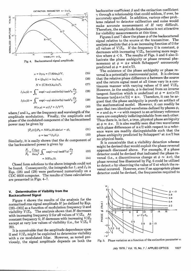
Figures 5 and 7 show the phase 0 of the backscatteredsignal relative to the source at the transmitter. Theanalysis predicts that 0 is an increasing function of Q forall values of VIZO. If the frequency Q is constant, 0

decreases with increasing V/Z0, becoming more nega-tive where 0 < 0. The results of Figs. 5 and 6 also il-lustrate the phase ambiguity or phase reversal phe-nomenon at 1 = h7r which Schappertl erroneouslypredicted at + = +n(-r/2).

The existence of the phase ambiguity or phase re-versal is a potentially controversial point. It is obviousthat the relative phase difference X between the sourceand the return signal must at all times vary in a con-tinuous manner with varying values of Q and V/Zo.However, in the analysis, 0 is derived from an inversetangent function which is undefined at 0 = +n(7r/2)because tan[±n(7r/2)] = Am. Therefore, it can be ar-gued that the phase ambiguity is purely an artifact ofthe mathematical model. However, it can readily beseen that two identical waveforms defined by phases 01= 7r and 102 = -ir with respect to an arbitrary referencewave are completely indistinguishable from each other.Thus there is, in fact, a true, physical phase ambiguityat 0 U i r. It is also readily seen that two waveformswith phase differences of +.ir/2 with respect to a refer-ence wave are readily distinguishable such that thephase ambiguity predicted by Schappert' at i r/2 hasno physical basis.

It is conceivable that a visibility detection schememight be devised that would exploit the phase reversalapproach discussed above. For example, if a phasedetector could be devised that indicated the phase re-versal (i.e., a discontinuous change at 0 ± 17r), thephase reversal line illustrated by Fig. 6 could be utilizedto detect a by observing the value of Q at which the re-versal occurred. However, even if an appropriate phasedetector could be devised, the frequencies required to

V. Determination of Visibility from theBackscattered Signal

Figure 4 shows the results of the analysis for thenormalized rms signal amplitude H [as defined by Eqs.(28)-(30)] as a function of modulation frequency Q and

visibility V/Z0. The analysis shows that H decreaseswith increasing frequency Q for all values of VIZO. Atconstant frequency Q, H decreases with increasing V/Z0except at very low values of visibility (i.e., for VIZO <20).

It is conceivable that the amplitude dependence uponQ and VIZ0 might be exploited to determine visibilitywith a cw modulated lidar. However, as noted pre-viously, the signal amplitude depends on both the

a

V')

Zna-

-3 N N -`1 -\1j-7r

Fig. 5. Phase variation as a function of the extinction parameter a.


1.0

o 0.90

N.: 0.8

cr

ca 0.7

o 0.6z

0.5

Ce

I

U-

-J 0.4C')WEULJ> 0.3

w~ 0.2

0L 0.1

0 2 4 6 8 10 12EXTINCTION PARAMETER a= 2yZ 0Fig. 6. The phase reversal line.

produce phase reversals corresponding to meterologicalvalues of a would be too high for practical implemen-tation. Therefore, we will also reject the phase reversalapproach and concentrate on the constant frequencycw lidar approach which is based upon the phase de-pendence in the range < r.

The data of Fig. 7 are the data of Fig. 5 but expandedin scale and restricted to values of 0 < r. Values of aand VZo are indicated on the upper and lower ordi-nates, respectively, and the signal phase is the ab-scissa. The predicted variation of with a is shown forseveral values of over a range of a values, which wouldbe of meterological interest (assuming reasonable valuesof Z). In practice, the visibility could be determinedby measuring the phase of the return signal relative tothe source where the appropriate value of VZ 0 couldthen be read from Fig. 7 at the appropriate value of themodulator frequency Q. It would, of course, be neces-sary to determine Zo for the optical system, establisha zero phase reference point, and optimize the systemin various ways that can be deduced from the analysis.

First, from Fig. 4 we see that for a given a, increasingvalues of Q correspond to decreasing values of the nor-malized amplitude H. This implies H 1/zof, andfrom Eqs. (27) and (31), P NH 1/zo3f. Therefore,from the standpoint of maximizing signal amplitude,we must design for the lowest practical frequency f, andthe optics should be designed to minimize the blockageparameter zo.

Second, from Fig. 7 we see that the proper choice ofQ also depends on the range of visibilities of interest tothe designer. The phase sensitivity of the instrument,which may be defined as the slope of the lines in Fig. 7,is highly dependent on Vzo for a given value of Q. Inparticular, it would be advantageous to choose a fre-quency corresponding to a value of on Fig. 7 so thatthe variation of V would always lie within the approxi-

mately log-linear region of the Q line chosen. If therange of V is larrge (i.e., if V varies by more than a factorof 10), it would be necessary to use two frequencies,corresponding to a high range and a low range withsufficient overlap to ensure adequate sensitivity overthe entire range.

VI. Signal Noise AnalysisFrom the experimental work of Lifsitz2 and from an

intuitive feel for the problem, it is obvious that thesignal from the cw lidar must be low level, at least forhigh visibility conditions. Therefore it will be usefulto delve deeper into the detection process to determinethe factors that affect the signal level and, more im-portantly, the signal-to-noise ratio (SNR) which ulti-mately determines the limits of measurement.Therefore, we will evaluate the sources and effects ofnoise in the signal in search of appropriate means fornoise reduction and signal enhancement.

There are a number of potential sources of noise thatmust be considered in evaluating the response of the cwmodulated lidar. Noise in the laser output, harmonicdistortion due to the modulator, and random atmo-spheric fluctuations would normally occur at very lowfrequencies, or at least at frequencies sufficiently re-moved from the modulation frequency that bandpassfiltering at the detector output should be adequate toeliminate noise from these sources. The effects ofbackscattering from spatial inhomogeneities might alsobe construed as noise, however, this aspect of theproblem will not be considered here. There is no reasonto expect appreciable noise in the amplifier or phasediscriminator circuitry so we will concentrate on noisegenerated in the photomultiplier.1 4 ,15

The detector dark current id is a spurious dc currentdue primarily to random thermionic emission. For atypical S-20 PMT at luminous sensitivity M 100-1000A/lm and a temperature of 300 K, id 2-50 nA. Thedark current may be virtually eliminated by cooling.However, since id is so small and since only ac infor-mation is sought, the effect of the dark current for thisstudy is negligible even without cooling.

The primary potential noise components in the out-

EXTINCTION PARAMETER a 2yz.l o- , l- , lo0_ _ -,

as.~~~~ 10 ° [

1.0~~~~0

wto *L./

II

10/

VISIBILITY V/Z.

Fig. 7. Variation of signal phase with visibility.

04


put are due to shot noise at the cathode and Johnsonnoise in the anode load resistor. The shot noise is dueto statistical variations in the photoemission process atthe cathode, which are in turn multiplied in the dynodestring. In addition, there are further statistical varia-tions in the dynode string which tend to increase thenoise even further. The total noise current due to shotnoise, Johnson noise, and secondary emission may begiven by 14

i= [ (2a2eGIa +-)J] , (35)

where a = secondary noise enhancement factor;e = electronic charge;

Af = detector (or postdetector) bandwidth;G = gain factor;Ia = mean anode current;K = Boltzman's constant;R = load resistance;T = absolute temperature.

The Johnson noise in the anode load resistor is pro-portional to the factor 4KT/e, which is equal to 0.1 forT = 300 K. Thus the shot noise is much greater thanthe Johnson noise provided that

G >> 0./(2RIaa2 ). (36)

Assuming typical values (G - 106, R = 50 Q, a - 1), this

is satisfied for anode currents greater than 1 nA whichis negligible for the present study. Consequently thenoise current is primarily shot noise which may be ap-proximated by

in {2 eGI. Afl1/2, (37)

where a is assumed to be one.The noise is thus proportional to the magnitude of the

mean anode current which is in turn proportional to the

average total radiant power incident upon the detector.The total radiant power Pt is P5, from Eq. (34), plus thebackground radiation PB, such that the average anodecurrent is given by

Ia = GSP, = GS(P, + PB), (38)

where S is the photocathode sensitivity in A/W at thelaser wavelength. The rms value of the ac detectorcurrent is given by

([s) = G.(-)S (Ps).

We will assume that the ac gain Ga (c) is equal to th

gain G for the frequency range of interest. The Sis then given by

SNR= '= GS (Ps)i, [2eG(GSPt) Af] 1 2

= (P0 ) [2(p 8- PB)Af ]

To illustrate the significance of the results ofsection, we will calculate an estimate of the theorelresponse of the modulated cw lidar which was testeiLifsitz.2 The pertinent data and the results ofcalculations are summarized in the first column of T

I. All the data used were obtained from Ref. 2 or i

(39)

e dcNR

(40)

(41)

thisticald bythe

able

mated on the basis of information given. The visibilitymeasurements were made in fog at visibilities of about15-60 m. There was no electronic filter after the de-tector; however, an amplifier in the circuit had a rolloffat about 10 MHz, effectively acting as a low-pass filter.

The calculated response parameters in Table I are forthe best conditions, which were actually encounteredin the experiment.

Additional evidence that the above estimate is rep-resentative of the actual system response is also givenin the report by Lifsitz.2 For the visibility conditionsemployed (V 50 m) and at a constant modulator fre-quency of 3 MHz, it was found that an increase in visi-bility by a factor of 2 was sufficient to cause signaldegradation to the extent that the phase discriminatorlost lock. It is obvious, therefore, that the SNR forLifsitz's system was indeed very close to 1, even for the

best of conditions, and it is certainly not surprising thatthe system did not function as expected. It is signifi-cant to note that the simple addition of a 1-kHz band-pass filter following the detector would have been suf-ficient to obtain a theoretical SNR of about 84, at whichthe system probably would have worked.

VII. Design of a Prototype cw Lidar

We may summarize the significant results of theanalysis of the theoretical response of the modulated cw

lidar as follows:(1) From Figs. 4-7, it is clear that the best technique

for measuring V would utilize the dependence of 1 uponV in the region of 0 < -r.

(2) Figure 4 shows that to maximize the signal am-

Table I. Design Data and Theoretical Responseof the Proposed cw Lidar as Compared to Lifsitz's System

Lifsitz system (2) Proposed system

.Source He-Ne laserX = 633 nmPO= 5 mW

Collector Refracting, F/5optics D = 12.7 cm

ZO 10 m (measured)

Detector Photomultiplierresponse: S-20S = 30 mA/W

at 633 nmG = 2 x 106

Modulator Electrooptic1 MHz < f < 10 MHzDm = 30%PO = 2 mWPO= 0.86 mW

Filters AX= 5 nmAf - 10 MHz(Amplifier rolloff)

Operating 0.03 6 2 0.3variables 0.06 6 VIZ0 6 0.26

(Actual experimentalconditions)

Theoretical ) - 1.7 X 10-loWresponse i,) - 5.2 X 10-6 A

SNR 0.84

He-Cd laserX = 442 nmPO= 5 mWFresnel, F/5D = 25 cmZO 10 m

Photomultiplierresponse: S-20S = 60 mA/W at

452 nmG = 2 x 106Acoustooptic0 < f < 1 MHzPm = 100%P0 = 2.5 mWP0= 2.5 mWAX= 3 nmAf = 1 kHz

(1) 2, = 0.0210 6 V/Z 0 < 10,

(2) 2, = 0.002102 6 VIZO 6 103

10-9 W(i- 2.5 X 10- ASNR 250


-

plitude, it is desirable to design for low frequency op-eration.

(3) From Fig. 5 we see that the modulation frequency/ should be carefully chosen to assure maximum sensi-tivity and range.

(4) From Fig. 4 and from Eqs. (27) and (31), we seethat Zo should be minimized since the signal level variesroughly as 1/z0

3 .(5) From Eq. (44) we see that it is important to match

the detector response to the laser wavelength, but weneed only use as much gain as is required to trigger thephase discriminator.

(6) From Eq. (44), we see that we need to use as muchlaser power as we can with maximum modulation depth.The detector window should contain a bandpass opticalfilter matched to the laser wavelength, and the detectorfield of view should be minimized.

(7) From Eq. (44) we see that the SNR is propor-tional to (f)1/ 2. Therefore the detector must outputthrough a narrowband electronic filter, or equivalently,a lockin amplifier might be employed in the detectorcircuit.

The choice of a laser for the system is subject to anumber of considerations. The power output of thelaser should be as high as possible, subject to limitationsof cost and eye safety. For practical applications underuncontrolled conditions where direct eye exposure ishighly probable, current safety regulations would surelylimit power levels to a few milliwatts or possibly as muchas 10-20 mW if the beam is expanded to reduce thespatial intensity. However, the experimental resultsof Lifsitz2 and the results of the present analysis indi-cate that about 5 mW of power is probably adequate forrelatively low visibility conditions in a properly designedcw lidar system.

The choice of laser wavelength is somewhat moresubjective. The maximum sensitivity of the human eye,is at about 550 nm which very nearly corresponds to thepeak sensitivity range of many photodetectors. Theintensity of scattering varies as -l to -4 in going frompurely aerosol scattering to Rayleigh scattering, which,of course, accounts for the blue haze that commonlyobscures visibility. Based on these considerations itseems that a laser in the midvisible region of the spec-trum might be most appropriate, perhaps a He-Cd laseror an Ar-ion laser. In some cases it might be advanta-geous to use a laser with several selectable wavelengthsor with continuously variable wavelengths as obtainedwith dye lasers.

The choice of a modulator is essentially limited to twoalternatives: electrooptic modulators (Pockells cells)or acoustooptic modulators (Bragg cells). Pockells cellstend to be rather difficult to work with but offer veryhigh frequency response. Bragg cells are inherentlysimpler and easier to work with but are limited tofrequencies of about 20 MHz or less. Since the presentanalysis indicates that frequencies of 1 MHz or lessshould be adequate for this application, it appears thatthe Bragg cell offers the best choice. It should be notedthat some lasers may be purchased with builtin modu-lation capability, which may offer the best overall so-lution.

The detector should be chosen to give maximumsensitivity at the chosen laser wavelength. An S-20multialkalian tube would be a good choice for theblue-green region giving a cathode sensitivity of up to95 mA/W and a current gain of up to 107 with ten-stageamplification. The narrowband optical filter shouldbe preceded by a collimating lens since only thosewavefronts which are very nearly parallel to the filtersurface are passed.

The collector optics should be as large in diameter aspossible since their purpose is to collect as much lightas possible from along the entire beampath. Since thecollection efficiency is the primary consideration (asopposed to image formation), a Fresnel lens might offerthe most cost-effective alternative. Standard refractingor reflecting optics could also be used if available, butthe added cost and the additional bulk required in thesystem would probably not be justified.

Ideally, the field of view of the collector should be asnarrow as possible to reduce the level of the backgroundradiation. This may be accomplished by baffles in thetelescope. However, the narrower the field of view, themore difficult it will be to maintain proper alignment.In addition, the blockage due to the mirror and thebaffling determine the magnitude of the parameter z0which is a measure of the length of the dead space infront of the lens from which scattering is effectivelyblocked from the detector. It is easily shown thatbaffling the telescope causes zo to increase, resulting ina reduction in signal amplitude (which goes approxi-mately as liz 3). However, increasing z also has thedesirable effect of reducing the degree to which themeasurements are weighted toward the near field visi-bility conditions. It will be necessary to experimentwith the optics to determine how much baffling is reallydesirable since the combined effect of lenses, baffles,filter, and blockage is just too complicated to deal withanalytically.

The electronics downstream from the detector arerelatively simple. An amplifier may be needed to assureadequate signal level to trigger the phase comparator.However, calculations indicate that sufficient amplifi-cation should be available in the photomultiplier. Theoutput filter is necessary to provide noise isolation, aspointed out above. It will be necessary to provide fre-quency variability to cover a broad range of visibilities.For this purpose, the oscillator, amplifier, and filtershould be tunable, or alternate fixed frequency com-ponents might be provided which could be accessedthrough a range switch.

There are at least two ways in which the actual phasecomparison may be done. A partial beam splitter anda second detector may be inserted following the mod-ulator from which a reference signal would be available,the technique that was used by Lifsitz.2 However, itwould be simpler to pick a reference signal directly offfrom the oscillator output as illustrated in Fig. 2. Ineither case it will be necessary to establish a zero-phaseshift calibration point from which all measurementsmay be referenced.

The actual phase comparison could be done visuallyon a dual trace oscilloscope. However, for most pur-


poses it would be more practical to use an instrumentspecifically designed for phase comparison purposes,such as the vector power meter used by Lifsitz. 2 A

lockin amplifier might be used as a phase detectorwithout the need for an additional filter. Alternatively,it would be relatively simple to synthesize a phase dis-

criminator from integrated circuit components whichare readily available and inexpensive. The signal out-put may be recorded on paper or tape depending in therequirements of the application.

The proposed cw lidar is illustrated in Fig. 2, and the

details of design and theoretical performance are sum-marized in Table I for comparison with the systemtested by Lifsitz.2 The most significant improvementsin the proposed system are the use of lower modulationfrequencies and the addition of the electronic filterand/or lockin amplifier. For the purpose of compari-son, we have assumed the same value of zo for both

systems although optimization with regard to zo iscertainly possible. The estimate of SNR for Lifsitz'ssystem was made for the case where maximum ampli-tude should have been achieved corresponding to very

low visibility (less than 50 m). The estimate of SNR for

the proposed system corresponds to the maximumamplitude that would be achieved at the upper limit ofthe stated visibility range of 10 km. The signal leveland SNR of the proposed system are theoretically more

than adequate for the proposed range of visibilities.

Vil. Conclusions

An analysis of the theoretical response of the modu-lated cw lidar proposed by Schappert has been per-formed that establishes the capabilities and limitationsof the technique for the measurement of atmosphericvisibility for homogeneous conditions. Deficiencies in

previous analyses and in the design of apparatus em-ployed in the only known experimental work on the

subject are identified, and appropriate corrections aresuggested. An improved modulated cw lidar is pro-posed for measurement of visibilities of up to 10 km or

more utilizing very modest source and detector speci-fications. Based on these estimates it appears that thecw modulated lidar is a potentially valuable techniquethat deserves further development.

The work described in this paper was performed bythe author while participating as a Senior ResearchFellow in the Advanced Study Program at the NationalCenter for Atmospheric Research, Boulder, Colorado.The author gratefully acknowledges the contributionsof G. W. Grams at NCAR who developed many com-puter codes employed in this study and who assisted innumerous other ways. Last, the author acknowledgesthe financial assistance of the National Science Foun-dation under whose auspices NCAR is funded.

References1. G. T. Schappert, Appl. Opt. 10, 2325 (1971).

2. J. R. Lifsitz, "The Measurement of Atmospheric Visibility with

Lidar: TSC Field Results," Report FAA-RD-74-29, U.S. De-

partment of Transportation, Systems Research and Development

Service, Washington, D.C. (1974).3. R. G. Buettell and A. W. Brewer, J. Sci. Instrum. 26, 357 (1949).

4. N. C. Ahlquist and R. J. Charlson, J. Air Pollut. Control Assoc.

17, 467 (1967).5. H. Howath and K. E. Noll, Atmos. Environ. 3, 543 (1969).

6. A. P. Waggoner, N. C. Ahlquist, and R. J. Charlson, Appl. Opt.

11,2886 (1972).7. R. T. H. Collis, Appl. Opt. 9, 1782 (1970).

8. R. T. Brown, "Backscatter Signature Studies for Horizontal and

Slant Range Vsibility," Report FAA-RD-67-24 or DDC-659-469

(1967).9. H. Koschmieder, Bier Phys. Frei. Atm. 12, 33 (1924).

10. M. Kerker, Scattering of Light and Other Electromagnetic Ra-

diation (Academic, New York, 1969).

11. W. E. K. Middleton, Vision Through the Atmosphere (Univ. of

Toronto, Toronto, 1958), Vol. 19, p. 203.

12. M. P. McCormick, J. D. Lawrence, and F. R. Crownfield, Appl.

Opt. 7, 2424 (1968).13. H. Harrison, J. Herbert, and A. P. Waggoner, Appl. Opt. 11, 2880

(1972).14. J. Sharp, "Photoelectric Cells and Photomultipliers," EMI

Electronics Ltd., Hayes, England (1961).

15. M. Ross, Laser Receivers (Wiley, New York, 1967).

Samuel Wesley Stratton (1861-1931)-left-was largely responsible for the establishment in 1901 of the National Bureau of Standards. He

was its first director, and continued in that position for more than twenty years. He died while dictating an encomium of his close friend Thomas

A. Edison. Thomas Alva Edison (1847-1931), inventor of the incandescent lamp, the phonograph, and the electric dynamo, was the greatest

inventive genius of his time-he patented over one thousand inventions. He had no academic scientific training, and his formal education

was limited to three months in a grammar school at Port Hudson, Michigan. He was thirty when he invented the electric light. Edward Bennett

Rosa (1861-1921)-right-joined Stratton, in 1902, at NBS as second in command and he died literally at his post-working in his office.

Coblentz wrote his biographical sketch for the National Academy of Sciences. Photos: E. S. Barr.


atmospheric visibility measurement by a modulated cw lidar

Documents