atmospheric simulations and their optimal control
TRANSCRIPT

Mitg
lied
de
r H
elm
ho
ltz-G
em
ein
sch
aft
Atmospheric Simulations and their Optimal Control
H. Elbern, E. Friese, L. Nieradzik, K. Kasradze, J. Schwinger
Chemical Data Assimilation group FZ Jülich, IEK-8
and Rhenish Institut of Environmental Research at the University of Cologne

13. August 2012 Folie 2
Outline
1. Optimisation: a universal scientific objective
2. Problem: How can we control a system with high
degrees of freedom?
3. How can we optimally combine models with
observations?
1. a means to upgrade our knowledge basis
2. test hypotheses
Specifically in atmospheric sciences:
1. for green house gas inversion
2. for air quality and climate monitoring/reanalyses
3. Extension: “detection and attribution” algorithm for climate
change
13. August 2012 Folie 3
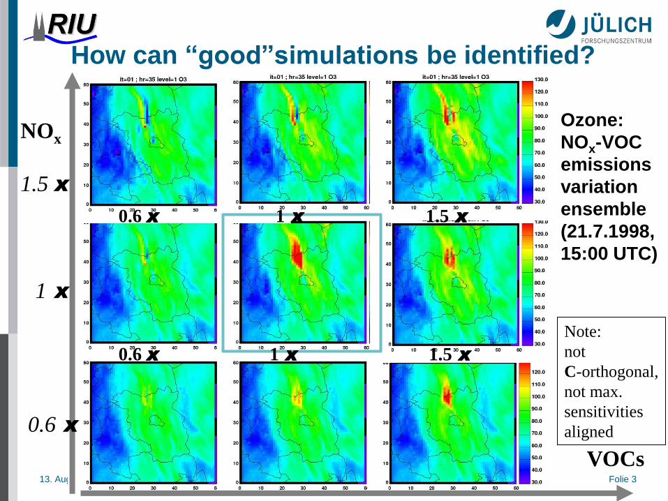
NOx
1.5 x
1 x
0.6 x
VOCs
Ozone:
NOx-VOC
emissions
variation
ensemble
(21.7.1998,
15:00 UTC)
Note:
not
C-orthogonal,
not max.
sensitivities
aligned
How can “good”simulations be identified?
0.6 x 1 x 1.5 x
0.6 x 1 x 1.5 x

13. August 2012 Folie 4
How can “good”simulations be identified?
Sequential Importance Resampling
How to select weights wi? time
extinct
survivors
obs.
Other techniques:
• Ensemble modelling
• (Markov Chain) Monte Carlo methods (MCMC)
• and many more versions …..

13. August 2012 Folie 5
Are there more focussed approaches?
e.g. quadratic optimisation
y
a
b { |
1
|
0 x
y=ax+b

13. August 2012 Folie 6
Isopleths of the cost function and
minimisation steps
Minimisation by mere gradients, quasi-Newon method L-BFGS
(Large dimensional Broyden Fletcher Goldfarb Shanno),
concentration species 1
concentr
ation s
pecie
s 2

13. August 2012 Folie 7
Extensions to Generality 1. very high degree of freedom of highly nonlinear systems M:
“curse of dimensionality” O(107-108)
2. underdetermined system: too few observations, i.e. less than
degrees of freedom
3. observations scattered in time and space,
4. different observation techniques:
errors and representativity of observations diverse
5. observations often indirectly related to parameters of interest:
remote sensing data
Methodology applicable to a wide range of problems:
Consider optimisation problem
with unique optimum
13. August 2012 Folie 8
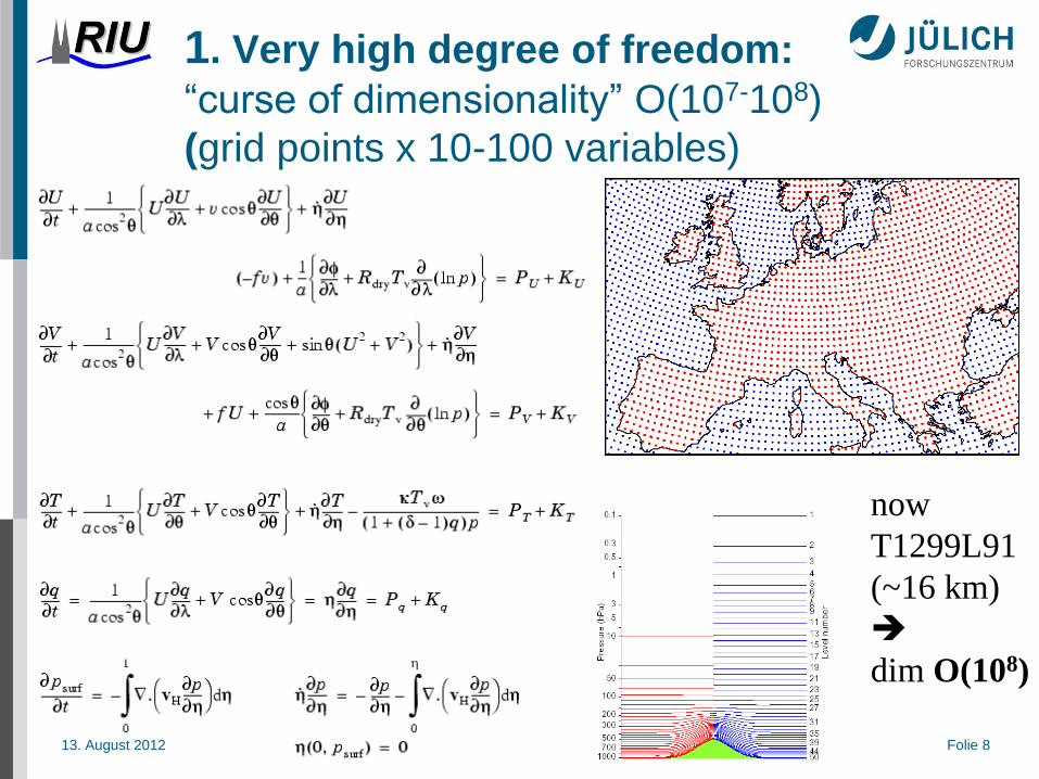
1. Very high degree of freedom:
“curse of dimensionality” O(107-108)
(grid points x 10-100 variables)
now
T1299L91
(~16 km)
dim O(108)

13. August 2012 Folie 9
1. Very high degree of freedom:
“curse of dimensionality” O(107-10-8)
(grid points x 10-100 variables)
3-D models
Example KAMM/DRAIS
KIT IMK (Karlsruhe)
SACADA icosahedral grid
(see presentation K. Kasradze)

13. August 2012 Folie 10
2. Underdetermined system: too few
observations, i.e. less than degrees of freedom
Type and number of
observations used to
estimate the
atmosphere initial
conditions during a
typical day.
(Buizza, 2000)
dimobservation space
<< O(107)
13. August 2012 Folie 11
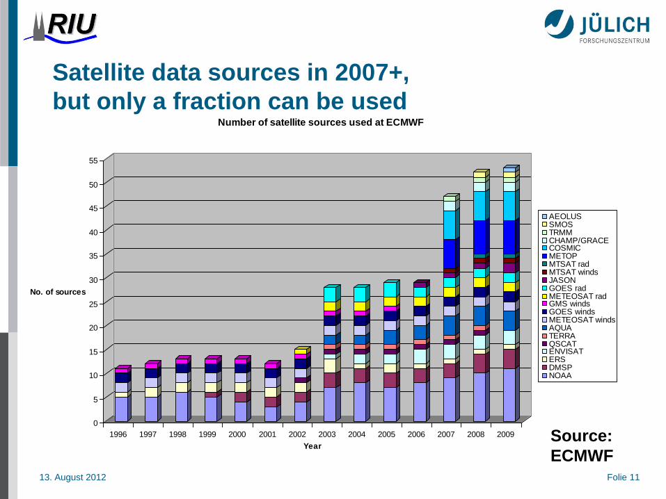
Satellite data sources in 2007+,
but only a fraction can be used
0
5
10
15
20
25
30
35
40
45
50
55
No. of sources
1996 1997 1998 1999 2000 2001 2002 2003 2004 2005 2006 2007 2008 2009
Year
Number of satellite sources used at ECMWF
AEOLUSSMOSTRMMCHAMP/GRACECOSMICMETOPMTSAT radMTSAT windsJASONGOES radMETEOSAT radGMS windsGOES windsMETEOSAT windsAQUATERRAQSCATENVISATERSDMSPNOAA
Source:
ECMWF

13. August 2012 Folie 12
Take the model for over-determination:
Synergy of information sources
a priori (=prediction or climatology) observation
Bayes’ rule:
xa
Analysis (=estimation) BLUE
Best Linear Unbiased Estimate
xb yo xa xb yo xb
Example: inconsistent data

13. August 2012 Folie 13
3. Observations scattered in time (and space)
MOZAIC - JAGOS Aeronet
LIDAR
MetOp-1 IASI, GOME-2
AIREP, AMDAR, ACAR

13. August 2012 Folie 14
4D-var
Kalman Filter
Types of assimilation algorithms:
“smoother” and filter y
a x
y=ax+b

13. August 2012 Folie 15
Transport-diffusion-reaction equation and its adjoint

13. August 2012 Folie 16
Adjoint integration “backward in time”
How to make the
parameters of resolvents i
M(ti-1,ti) available in reverse
order??

13. August 2012 Folie 17
CONTRACE Convective Transport of Trace Gases into the upper
Troposphere over Europe: Budget and Impact of
Chemistry
Coord.: H. Huntrieser, DLR
flight path Nov. 14, 2001
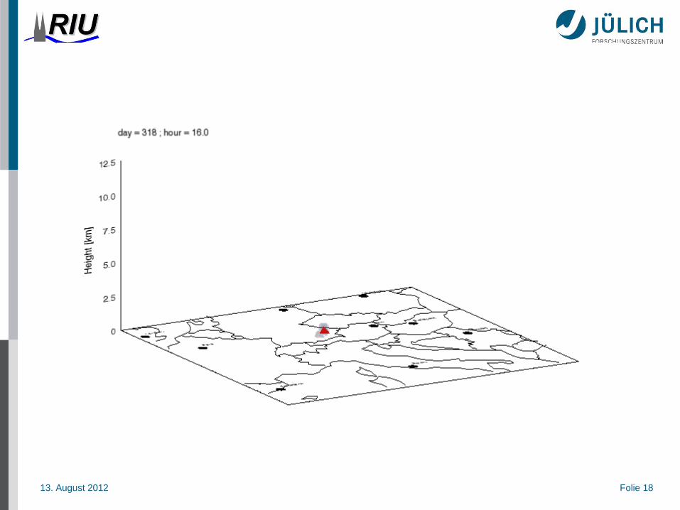
13. August 2012 Folie 18

13. August 2012 Folie 19
CONTRACE Nov. 14, 2001 north (= home) bound
O3
H2O2
CO
NO
1. guess assimilation result observations flight height [km]
13. August 2012 Folie 20
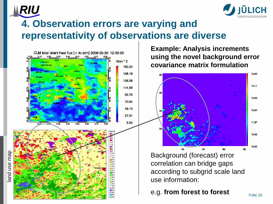
4. Observation errors are varying and
representativity of observations are diverse
Background (forecast) error
correlation can bridge gaps
according to subgrid scale land
use information:
e.g. from forest to forest
Example: Analysis increments
using the novel background error
covariance matrix formulation
lan
d u
se
ma
p

13. August 2012 Folie 21
5. Observations often indirectly related to
parameters of interest: Remote sensing
level 0: detector tensions:
digital data
level 1: calculate
spectra
level 2: calculate located
geo data (say: y=[NO2] )
level 3: “analysis
fields” (say NO2)
Example:
SCIAMACHY
Retrieval:
Solve the model equivalent:
radiative transfer equation H(x)
Calculate difference (y – H(x)),
and assimilate

13. August 2012 Folie 23
ENVISAT SCIAMACHY,
GOMOS;
MIPAS
AATSR
TERRA MOPITT, MODIS
MetOp-1 IASI, GOME-2
AURA OMI, HRDLS, MLS, TES
AQUA AMSR-E, MODIS, AMSU
AIRS, HSB, CERES
A train
AQUA (2002) AMSR/E: clouds,
radiation and precipitation ,
MODIS: clouds, radiation,
aerosol and vegetation
parameters , AMSU, AIRS, HSB
temperature and humidity,
CERES radiation
Main observational data (spaceborne)
AURA (2004) MLS trace gases of
the upper troposphere to upper
stratosphere, + water HIRDLS,
temperature and trace gases in the
upper troposphere, stratosphere and
mesosphere TES trop. ozone and
some photochemical precursors ;
OMI total column ozone and NO2
and UV-B radiation .
ENVISAT (2002-2012) MIPAS,
SCIAMACHY, GOMOS
temperature, ozone, water vapour
and other atmospheric constituents
(ii) AATSR, MERIS aerosoll,
MERIS sea colour , ASAR land
and ocean images RA-2 land, ice
and ocean monitoring, MWR water
vapour column and land surface
parameters DORIS cryosphere
and land surface parameters
TERRA (1999).ASTER,land
surface, water and ice,
CERES radiation, MISR
radiation and biosphere
parameters; MODIS biological
and physical processes on
land and the ocean; MOPITT
CO and CH4 in the
troposphere, .
MetOp-1
IASI
ozone,
NO2,
GOME-2
ozone
SO2 NO2
formaldeh
de

13. August 2012 Folie 24
Satellite information:
ESA UV-VIS satellite footprints Ruhr area comparison
minimal areas:
GOME 1 320 x 40 km2
(special mode) 80 x 40 “
SCIAMACHY 60 x 30 “
GOME 2 80 x 40 “
OMI 24 x 13 “
Ruhr area domain 90 x 80 km2
1 km resolution
(~12 000 000 inhabitants)

13. August 2012 Folie 26
Generalized cost function to be minimized
4. Observation errors
and
errors of representativity
3. Forecast errors
1. Model constraint and
time propagator (resolvent)
5. Observation operator
2. Background term for
artificial over-determination

13. August 2012 Folie 27
Question: Which parameter to be optimized?
Hypothesis:
initial state and emission rates are least known
emission biased model state
only emission rate opt.
only initial value opt.
true state
observations
time
conce
ntr
atio
n
joint opt.

13. August 2012 Folie 28
Terminology
Inverse Modelling
The inverse modelling problem consists of using the actual result of
some measurements to infer the values of the parameters that
characterize the system.
A. Tarantola (2005)
13. August 2012 Folie 29
Data Assimilation in general
The ambitious and elusive goal of data assimilation is to
provide a dynamically consistent motion picture of the
atmosphere and oceans, in three space dimensions, with
known error bars.
M. Ghil and P. Malanotte-Rizzoli (1991)
13. August 2012 Folie 30
Objective of atmospheric data assimilation
"is to produce a regular, physically consistent four dimensional representation of the state of the system
from a heterogeneous array of in situ and remote instruments
which sample imperfectly and irregularly in space and time.
Data assimilation
extracts the signal from noisy observations (filtering)
interpolates in space and time (interpolation) and
reconstructs state variables that are not sampled by the observation network (completion).“ (Daley, 1997)

13. August 2012 Folie 31
Emissionen
Deposition
radiation
Information sources and theories
•contol theory
•statist. filter theory
•classical numerics
•optimisation algorith.
Interpolation
in space and time
Filter
error affected
data
Completion
non-observed
parameters
Information set
declarative information:
•observations/retrievals
•forecasts
•“Climate” statistics,
•error statistics
procedural Information
differential equations
models
Ad
ve
ctio
n
4D-consistent
process description
aeroso
ls
aqueou
s
phase
chem.
micro-
physics
gas-
phase

13. August 2012 Folie 32
NOx
1.5 x
1 x
0.6 x
VOCs
0.6 x 1 x 1.5 x
0.6 x 1 x 1.5 x
Ozone:
NOx-VOC
emissions
variation
ensemble
(21.7.1998,
15:00
UTC)
Note:
not
C-orthogonal,
not max.
sensitivities
aligned
How can I select “good”simulations?
13. August 2012 Folie 33
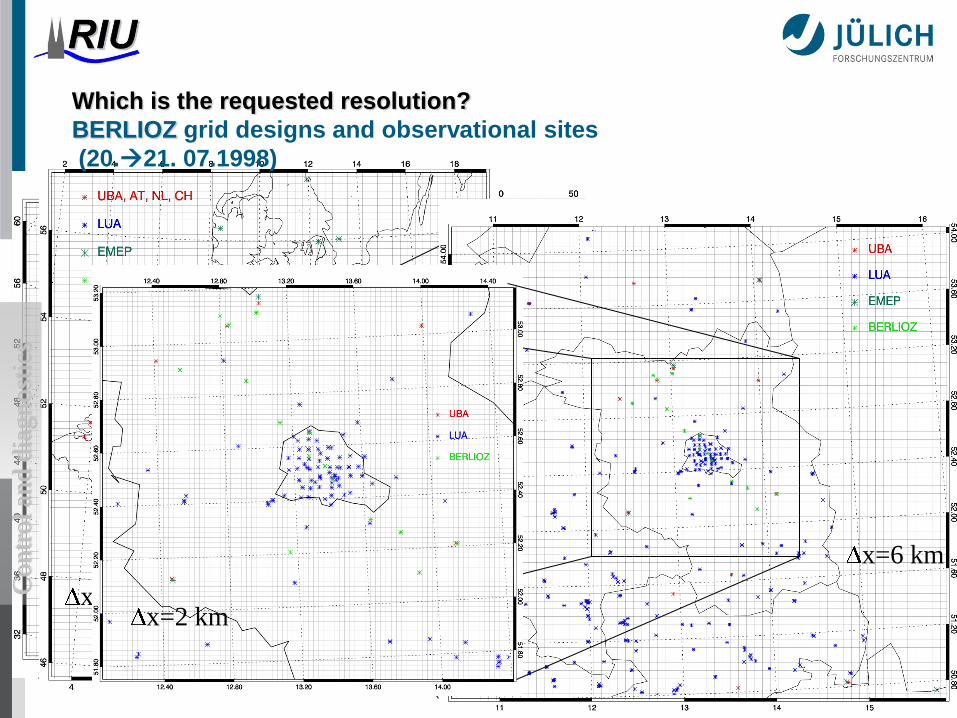
x=54 km
Which is the requested resolution?
BERLIOZ grid designs and observational sites
(20.21. 07.1998)
x=18 km
x=6 km
x=2 km
Co
ntr
ol
and
dia
gn
ost
ics

13. August 2012 Folie 34
Some BERLIOZ examples of
NOx assimilation (20.21. 07.1998)
NO
NO2
Time series for selected NOx
stations on nest 2.
+ observations,
-- - no assimilation,
-____ N1 assimilation (18 km),
-____N2 assimilation.(6 km),
-grey shading: assimilated
observations, others
forecasted.

13. August 2012 Folie 35
surf
ace
hei
ght
layer
~32
-~70m
NO2, (xylene (bottom), CO (top) SO2 .
Emission source estimates by inverse modelling
Optimised emission factors for Nest 3

13. August 2012 Folie 36
Nest 2: (surface ozone)
(20.21. 07.1998) without
assimilation with assimilation

13. August 2012 Folie 45
2. Analyses, Example (ii):
Zepter 2: 4D-var assimilation of particle number densities Flight 14 assimilation of PND (0.005-3.0 µm) 02.11.2008 (11-15 UTC)
First Guess
Analysis
Measurement
airship altitude
terrain height
PN
D [cm
-3]
Altitu
de
[m]
(from Lars Nieradzik, PhD thesis 2011)
water solubles include Friese and Ebel, 2010:
Lake Constance
flight domain

13. August 2012 Folie 46
2. Analyses, Example (ii cntd.):
Flight 14 assimilation of PND (0.005-3.0 µm), Nov. 2 Analysis increment (Analysis – Background)
Aitken mode PND Acc. mode PND
(~ 450m a.g.) 4 hour assimilation
5 km grid
from Lars Nieradzik, PhD thesis 2011

13. August 2012 Folie 48
Thank you for your attention!

13. August 2012 Folie 49
2 Questions:
1. Spatial optimisation only (no time evolution involved): How
does a closed formula for the optimum read?
2. Temporal optimisation: How can we integrate “backward in
time” with an adjoint model MT for an optimum at initial time?