SOLA, 2009, Vol. 5, 029‒032, doi:10.2151/sola.2009‒008

Abstract

Sounding data from the South China Sea MonsoonExperiment (SCSMEX) have provided a unique opportu-nity to document the variability of atmospheric mixedlayers over the South China Sea (SCS) during the onsetof the monsoon in this region. Six-hourly sounding datafrom two research vessels, deployed over the northernand southern SCS, are used to determine the mixed-layer depth and its thermodynamic properties.

Results from the southern ship show the presence ofmixed layers 83% of the time with a mean depth of 459m, similar to other tropical oceanic locations. On theother hand, the northern ship exhibited mixed layers48% of the time with a mean depth of 342 m, considera-bly less frequent and shallower than other tropicalregions. This anomalous behavior, which was particu-larly evident after the monsoon onset, is likely due tonorthward advection of low-level warm, moist air overcooler waters, which results in very small or negativebuoyancy fluxes over the northern SCS, and thus weakupward mixing of heat and moisture from the surface.

1. Introduction

During the onset of the Southeast Asian SummerMonsoon (SEAM), convection establishes itself overSouthern China and the northern SCS. With theultimate goal of obtaining a comprehensive descriptionof the SEAM to improve its predictability, SCSMEX wasdesigned to investigate the processes associated withthe monsoon onset and development during May andJune, 1998. An important aspect of the monsoon in thisregion is the coupling between the ocean and the atmos-phere. Since the atmospheric mixed layer (generally thelowest 0.5 km of the troposphere) is the mediumthrough which the ocean and the free atmosphere arecoupled, this study documents the properties and evolu-tion of the mixed layer over the SCS during SCSMEX.

2. Data sources and procedure for determin-ing mixed layers

During the SCSMEX intensive observing period(IOP) from 5 May to 22 June, two sounding networks(Fig. 1) were established over the SCS to determine andcontrast the properties of convection in two distinctocean regions of the SEAM. An integral part of thesenetworks were two research vessels (R/Vs) whichprovided hourly surface fluxes in addition to four high-vertical resolution sondes per day. The northernsounding array was centered around the R/V Shiyan 3,which was nominally located at 20.4°N, 117°E. The R/VKexue 1 was located on the perimeter of the southernarray at 6.2°N, 110°E. Hereafter we shall refer to thesesites as Ship 3 and Ship 1, respectively. These shipswere on location for the entire IOP except for a 9-day

port call near the end of May. Also shown in Fig. 1 is theSST analysis for this period based on the TRMM micro-wave imager (TMI) product (Wentz et al. 2000). Therainfall estimates used in this paper were obtained fromthe 3-h, 0.25° TRMM 3B42 version 6 TMI/IR mergedrainfall product (Huffman et al. 2007). Surface fluxeswere computed from ship observations and supple-mented with fluxes from the Japan MeteorologicalAgency (JMA) Global Energy and Water cycle EXperi-ment (GEWEX) Asian Monsoon Experiment (GAME)V1.1 special reanalysis for the SCSMEX.

For the analysis in this study we used 5-hPa verticalresolution (1005, 1000 hPa, ect.) sounding data. Bothsounding sites used Vaisala RS80 sondes. The overalldata quality at these sites appeared to be quite good,although the humidity data likely contain a daytimedry bias (Cady-Pereira et al. 2008) that was not cor-rected here. However, as noted in Johnson et al. (2001;hereafter JCC01), this type of error will not alter the de-termination of the mixed-layer depth which relies onvertical gradient information.

In this study, a subjective technique, using both po-tential temperature (�) and specific humidity (q) profiles,was used to identify mixed-layer tops. This techniquewas used to identify mixed layers over the westernPacific using sounding data from the Tropical OceanGlobal Atmosphere Coupled Ocean-Atmosphere Experi-ment (TOGA COARE) as described in JCC01. Specifi-cally, the mixed-layer top or inversion base (zi) isidentified as the level at which �exhibits an abruptincrease with height (with a near constant value below)and q has a sharp decrease with height (following aslight decrease or constant value below). Both of thesestructures must be present for a sounding to be assigneda zi. Details of this technique along with examples of theprocedure can be found in JCC01. By using 5-hPa (~50m) resolution data in this study, zi can be determined towithin ~50 m.

29

Atmospheric Mixed Layers over the South China Sea during SCSMEX

Paul E. Ciesielski and Richard H. Johnson

Department of Atmospheric Science, Colorado State University, Fort Collins, Colorado, USA

Corresponding author: Paul E. Ciesielski, Department ofAtmospheric Science, Colorado State University, Fort Collins,Colorado 80523, USA. E-mail: paulc@atmos.colostate.edu.©2009, the Meteorological Society of Japan.

Fig. 1. Map of SCSMEX sounding network showing the loca-tion of sounding sites (gray circles with R/Vs denoted by whitecircles). Color shading shows the SST field for the SCSMEXIOP with scale to right.

Ciesielski and Johnson, Mixed Layers in SCSMEX

3. Mean properties of the mixed layer

The IOP-mean properties of the mixed layers for thetwo sites in question are listed in Table 1. The meanheight for Ship 1 of 459 m is similar to what wasobserved in other tropical regions (424 m in GATE, 512m in TOGA COARE, JCC01). The frequency of mixedlayers at Ship 1 of 83% is somewhat higher than the 72%observed in TOGA COARE. On the other hand, the meanmixed-layer height and frequency for Ship 3 of 342 mand 48%, respectively, are considerably lower than thatfound in other tropical regions. The standard deviationof zi at both sites is quite similar (~110 m) and considera-bly smaller than that observed in TOGA COARE (~155m). The larger variability in COARE is likely related tothe buildup and decay of westerly wind bursts (WWBs),occurring on intraseasonal time scales, during whichconvective conditions and associated processes affect-ing mixed-layer depth varied substantially. Whileconvectively active and suppressed periods wereobserved during SCSMEX (see rainfall time series inFigs. 4 and 5), the range of conditions over the SCS waslikely not as large as that observed in TOGA COARE.

The histograms of the mixed-layer tops for the twosites are shown in Fig. 2. The characteristics of the his-togram for Ship 1 (namely, the higher mean and thenormal shape of the distribution) are quite similar tothose observed in TOGA COARE (JCC01). The preva-lence of shallow mixed layers at Ship 3 results from acombination of factors including weaker buoyancyfluxes, heavier rainfall events and/or a higher fre-quency of shallow, recovering precipitation downdraftwakes near this site.

By scaling each profile by its mixed-layer depth in

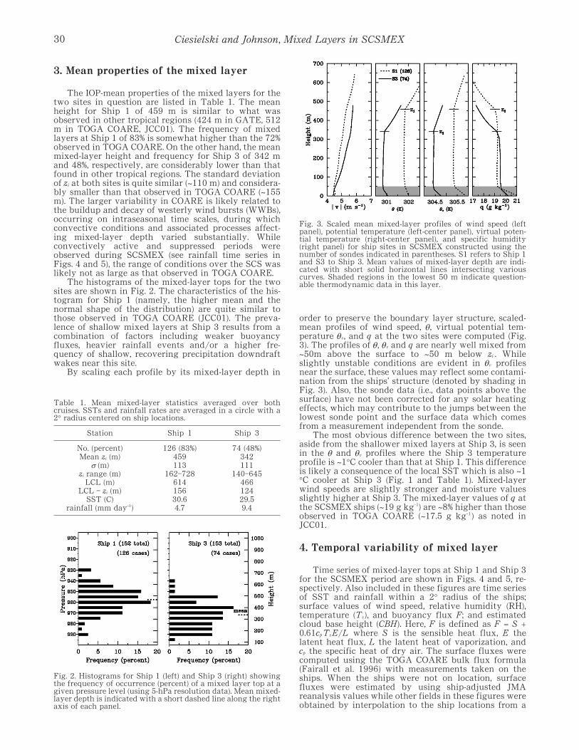
order to preserve the boundary layer structure, scaled-mean profiles of wind speed, �, virtual potential tem-perature �v, and q at the two sites were computed (Fig.3). The profiles of �, �v and q are nearly well mixed from~50m above the surface to ~50 m below zi . Whileslightly unstable conditions are evident in �v profilesnear the surface, these values may reflect some contami-nation from the ships’ structure (denoted by shading inFig. 3). Also, the sonde data (i.e., data points above thesurface) have not been corrected for any solar heatingeffects, which may contribute to the jumps between thelowest sonde point and the surface data which comesfrom a measurement independent from the sonde.

The most obvious difference between the two sites,aside from the shallower mixed layers at Ship 3, is seenin the �and �v profiles where the Ship 3 temperatureprofile is ~1°C cooler than that at Ship 1. This differenceis likely a consequence of the local SST which is also ~1°C cooler at Ship 3 (Fig. 1 and Table 1). Mixed-layerwind speeds are slightly stronger and moisture valuesslightly higher at Ship 3. The mixed-layer values of q atthe SCSMEX ships (~19 g kg‒1) are ~8% higher than thoseobserved in TOGA COARE (~17.5 g kg‒1) as noted inJCC01.

4. Temporal variability of mixed layer

Time series of mixed-layer tops at Ship 1 and Ship 3for the SCSMEX period are shown in Figs. 4 and 5, re-spectively. Also included in these figures are time seriesof SST and rainfall within a 2° radius of the ships;surface values of wind speed, relative humidity (RH),temperature (Ts), and buoyancy flux F; and estimatedcloud base height (CBH). Here, F is defined as F = S +0.61cp Ts E/L where S is the sensible heat flux, E thelatent heat flux, L the latent heat of vaporization, andcp the specific heat of dry air. The surface fluxes werecomputed using the TOGA COARE bulk flux formula(Fairall et al. 1996) with measurements taken on theships. When the ships were not on location, surfacefluxes were estimated by using ship-adjusted JMAreanalysis values while other fields in these figures wereobtained by interpolation to the ship locations from a

30

Table 1. Mean mixed-layer statistics averaged over bothcruises. SSTs and rainfall rates are averaged in a circle with a2° radius centered on ship locations.

Station Ship 1 Ship 3

No. (percent)Mean zi (m)

�(m)zi range (m)

LCL (m)LCL ‒ zi (m)

SST (C)rainfall (mm day‒1)

126 (83%)459113

162‒72861415630.64.7

74 (48%)342111

140‒64546612429.59.4

Fig. 2. Histograms for Ship 1 (left) and Ship 3 (right) showingthe frequency of occurrence (percent) of a mixed layer top at agiven pressure level (using 5-hPa resolution data). Mean mixed-layer depth is indicated with a short dashed line along the rightaxis of each panel.

Fig. 3. Scaled mean mixed-layer profiles of wind speed (leftpanel), potential temperature (left-center panel), virtual poten-tial temperature (right-center panel), and specific humidity(right panel) for ship sites in SCSMEX constructed using thenumber of sondes indicated in parentheses. S1 refers to Ship 1and S3 to Ship 3. Mean values of mixed-layer depth are indi-cated with short solid horizontal lines intersecting variouscurves. Shaded regions in the lowest 50 m indicate question-able thermodynamic data in this layer.

SOLA, 2009, Vol. 5, 029‒032, doi:10.2151/sola.2009‒008

1° gridded dataset. The procedures for adjusting thefluxes and creating the gridded dataset are described inJohnson and Ciesielski (2002). Notably, JMA fluxes col-located to those observed at Ship 3 were ~80 W m‒2

higher than those observed in the post-onset period. Theshading at the bottom of Figs. 4a and 5a indicates whenthe ships were on location and had successful sondelaunches. The parameter CBH in meters is computed asCBH = 125*(Ts‒Td) from Stull (1995, p. 88), where Td isthe surface dew point temperature. The monsoon onset,as determined by a shift in the low-level winds (Wang etal. 2004 used 850 hPa winds) from easterly to south orsouthwesterly over the SCS, occurred around mid-May(also see wind barbs in Figs. 4b and 5b).

The time series of fields for Ship 1, with mixed layerspresent 83% of the time, are typical of other tropicallocations as noted earlier. While surface wind speedsaveraged ~25% less at Ship 1 (Figs. 4b and 5b), surfacefluxes were more than double at this site compared tothose observed at the Ship 3. As noted in Ciesielski andJohnson (2006), this was due to larger air-sea tempera-ture (Fig. 4c) and moisture gradients over the southernSCS. The magnitude of the IOP-mean total surface flux(S+E) at Ship 1 of 112 W m‒2 (Ciesielski and Johnson2006) is comparable to the time-mean observed over theintensive flux array (IFA) in TOGA COARE (115 W m‒2,Johnson and Ciesielski 2000). Cloud bases variedbetween 500 and 650 m at Ship 1 with periods ofheavier rain (during cruise 2) characterized by zi extend-ing up to CBH, which promotes cloud development asovershooting boundary layer plumes or thermalsapproach the lifting condensation level (LCL). Typicalof other tropical regions, the surface RH field near Ship1 varied between 74 and 80% (Fig. 4d).

During its first cruise, suppressed convection (meanrain rate of 0.9 mm day‒1 ) and lighter winds werepresent in the vicinity of Ship 1 (Figs. 4b and 4d). Underthese conditions, which were also observed in pre-

westerly wind burst periods in TOGA COARE (JCC01),variability in the mixed-layer top was somewhat dimin-ished, being affected primarily by radiatively drivendiurnal effects. Cruise 1 mixed-layer tops at Ship 1varied by 58 m (or 13%) from day to night with depthsmaximizing in the afternoon (14 LT) and evening (20LT) soundings. A more detailed analysis of the diurnalcycle of the boundary layer during SCSMEX can befound in Yu et al. (2009a).

Enhanced convective activity (with a mean rain rateof 9.1 mm day‒1) was observed during the second cruiseat Ship 1 which led to greater variability in mixed-layertops. As seen in Fig. 4c, the SST continued to rise duringthis period while Ts slowly decreased likely from con-vective downdrafts transporting cool, dry air towardsthe surface. In response, surface buoyancy fluxespeaked during cruise 2 (Fig. 4b).

While the conditions at Ship 1 are more typical ofother oceanic tropical regions, those at Ship 3, particu-larly during its second cruise, are quite anomalous (Fig.5). Precipitation in the vicinity of Ship 3 shows twoconvectively active periods over the northern SCS; thefirst, centered around mid-May, was associated with themonsoon onset in this region, and a second period witheven higher rain rates was observed in early June. Priorto the monsoon onset, clear skies and low-level east-erlies resulted in warmer conditions over the northernSCS as evidenced by the ~1°C Ts rise and ~2°C SST rise(Fig. 5c). The greater SST increase resulted in a modest,positive surface buoyancy flux during this period (Fig.5b). Immediately following the rainfall peak in mid-May,mixed-layer depths decreased dramatically for about a5-day period. Such shallow boundary layers duringperiods of heavy rainfall, also noted in SCSMEX by Yuet al. (2009b), are likely related to recovering precipita-tion downdraft wakes in regions of convective rainfall(Young et al. 1995). The frequency of mixed layersduring the first cruise of Ship 3 is 75% which is typicalof other oceanic tropical regions. However, during itssecond cruise only 20% (15 out of 75) of the soundingsshowed a mixed-layer structure.

Conditions during the second cruise at Ship 3 arecharacterized by northward advection of warm, moistair. As one can note in Fig. 5, Ts tendencies at thislocation are affected by the wind direction such that

31

Fig. 4. Time series of various fields from Ship 1. Panel (a) showsmixed-layer tops (tops of vertical solid bars) and estimatedcloud base height (cyan line) where dark-shaded regions atbottom of this panel indicate times at which soundings weretaken; (panel b) surface wind speed (heavy line with scale toleft), buoyancy flux (red line with scale to right) and surfacewind barbs (with speed in knots); (panel c) Ts (dashed) and SST(solid); (panel d) surface RH (heavy line with scale to left) andrainfall (green line with scale to right). All fields except zi havebeen filtered with a 5-day running mean.

Fig. 5. As in Fig. 4, except for Ship 3.

Ciesielski and Johnson, Mixed Layers in SCSMEX

surface warming (cooling) generally occurs with south-erly (northerly) flow. While the SST field continues toslowly warm, much of this period is characterized byTs > SST (Fig. 5c). Despite the higher wind speedsduring this time, the weak or reversed temperaturegradient results in small or negative buoyancy fluxes(Fig. 5b) and few mixed layers. The mixed layers whichformed during this period of negative F were likely aresult of shear-generated turbulence, cloud-top radiativecooling, or horizontal advection of mixed layers fromthe upwind region. Extremely high RHs (> 85%) and lowcloud bases (300‒400 m) were also present throughoutmuch of the second cruise. To our knowledge suchanomalous conditions, resulting in negative buoyancyfluxes, weak vertical mixing and a lack of mixed layers,have not been observed in other oceanic subtropicalregions.

To further examine the conditions leading to theabsence of mixed layers at Ship 3, Fig. 6 shows thevertical profiles of wind speed and thermodynamic vari-ables in the lower troposphere from Ship 3 soundingswhen no mixed-layer structures were present. In con-trast to the mean mixed-layer profiles from Ship 3 inFig. 3, the profiles in Fig. 6 show q decreasing and �, �v

increasing monotonically from the surface upward. Inaddition, these periods with no mixed layers were char-acterized at low levels by higher wind speeds (up to 2 ms‒1), twice the vertical shear, warmer temperatures (1°C)with stable lapse rates, and moister air (1‒1.5 g kg‒1). Thehigher wind shear in Fig. 6 is consistent with lessvertical mixing.

5. Summary and concluding remarks

High-vertical resolution soundings (305 total) fromthe R/V Kexue 1 and Shiyan 3 have been used to deter-mine the properties of the atmospheric mixed layer overthe South China Sea during SCSMEX. While the mixed-layer behavior (mean depth 459 m, frequency 83%) andatmospheric conditions at the southern Ship 1 weresimilar to those of other oceanic tropical regions, suchwas not the case at the northern Ship 3 (mean depth 342m, frequency 48%). Following a period of heavy rainfallassociated with the monsoon onset, and particularlyduring its second cruise, a warm, moist low-level south-erly flow over cooler waters resulted in very small ornegative surface buoyancy fluxes at Ship 3. These weakfluxes are likely the reason for the infrequent andshallow mixed layers at this site.

Whether the anomalous mixed-layer featuresobserved at Ship 3 during SCSMEX occur in othermonsoon regions and seasons is uncertain. However, apreliminary examination of dropsondes and ship sound-ings upstream of Taiwan during TiMREX (Terrain-influenced Monsoon Rainfall Experiment) conducted inMay and June, 2008 exhibited some similar features.Most notably, several soundings taken in conditions ofa low-level moist southwesterly flow showed an absenceof mixing in the Td profile with moisture increasingmonotonically towards the surface (C. Davis 2008personal communication).

Finally, the large difference noted in the JMAreanalysis fluxes and those observed at Ship 3 in thepost-onset period suggest that models may have diffi-culty in reproducing the correct boundary layer struc-tures under weak stability conditions and may need todeal with such boundary layers differently to produceaccurate predictions of lower-atmospheric variabilityand convection.

Acknowledgments

This research has been supported by the NationalAeronautics and Space Administration (NASA) undergrant NNX07AD35G. We thank Dr. Chris Davis whoseearly assessment of the TiMREX sonde data motivatedus to undertake this study.

References

Cady-Pereira, K. E., M. W. Shephard, D. D. Turner, E. J. Mlawer,S. A. Clough, and T. J. Wagner, 2008: Improved daytimecolumn-integrated precipitable water vapor from Vaisalaradiosonde humidity sensors. J. Atmos. Oceanic Technol.,25, 873‒883.

Ciesielski, P. E., and R. H. Johnson, 2006: Contrasting character-istics of convection over the Northern and SouthernSouth China Sea during SCSMEX. Mon. Wea. Rev., 134,1041‒1062.

Fairall, C. W., E. F. Bradley, D. P. Rodgers, J. B. Edson, and G. S.Young, 1996: Bulk parameterization of air-sea fluxes forTOGA COARE. J. Geophys. Res., 101, C2, 3747‒3764.

Huffman, G. J., R. F. Adler, S. Curtis, D. T. Bolvin, and E. J.Nelkin, 2007: Global rainfall analysis at monthly and 3-hrtime scales. Measuring Precipitation from Space:EURAINSAT and the Future. V. Levizzani, P. Bauer, and JTurk, Eds., Kluwer Academic, 291‒306.

Johnson, R. H., P. E. Ciesielski, and J. A. Cotturone, 2001: Multi-scale variability of the atmospheric mixed layer over theWestern Pacific warm pool. J. Atmos. Sci., 58, 2729‒2750.

Johnson, R. H., and P. E. Ciesielski, 2002: Characteristics of the1998 monsoon onset over the northern South China Sea.J. Meteor. Soc. Japan, 80, 561‒578.

Stull, R. B., 1995: Meteorology Today: For Scientist andEngineers. West Publishing, 385 pp.

Wang, B., L. Ho, Y. Zhang, and M.-M. Lu, 2004: Definition of theSouth China Sea monsoon onset and commencement ofthe East Asia summer monsoon. J. Climate, 17, 699‒710.

Wentz, F. J., C. Gentemann, D. Smith, and D. Chelton, 2000:Satellite measurements of sea surface temperaturethrough clouds. Science, 288, 847‒850.

Young, G. S., S. M. Perugini, and C. W. Fairall, 1995: Convectivewakes in the equatorial western Pacific during TOGA.Mon. Wea. Rev., 123, 110‒123.

Yu, X., Q. Xie, and D. Wang, 2009a: The diurnal cycle of marineboundary layer during the summer monsoon over theSouth China Sea in 1998. J. Tropical Ocean., 27(4), (inpress).

Yu, X., Q. Xie, W. Zhou, X. Wang, and D. Wang, 2009b:Characteristics of marine atmospheric boundary layer as-sociated with the summer monsoon onset over the SouthChina Sea in 1998. Chinese J. Oceanol. & Limnol., 26(6), (inpress).

Manuscript received 2 December 2008, accepted 2 February 2009SOLA: http://www.jstage.jst.go.jp/browse/sola/

32

Fig. 6. Lower-troposphere mean profiles of wind speed (leftpanel), potential temperature (left-center panel), virtual poten-tial temperature (right-center panel) and specific humidity(right panel) for Ship 3 when no mixed layers were present atthis site.