Atmospheric aerosol backscatter measurements usinga tunable coherent CO2 lidar

Robert T. Menzies, Michael J. Kavaya, Pierre H. Flamant, and David A. Haner

Measurements of atmospheric aerosol backscatter coefficients, using a coherent CO2 lidar at 9.25- and 10.6-,um wavelengths, are described. Vertical profiles of the volume backscatter coefficient fl have been mea-sured to a 10-km altitude over the Pasadena, Calif., region. These measurements indicate a wide range ofvariability in 13 both in and above the local boundary layer. Certain profiles also indicate a significant en-hancement in fl at the 9.25-jm wavelength compared with 13 at the 10.6-jim wavelength, which possibly indi-cates a major contribution to the volume backscatter from ammonium sulfate aerosol particles.

I. IntroductionThe measurement of atmospheric aerosol backscatter

coefficients at CO2 laser wavelengths has been receivingincreased attention during the past few years. Thereare several reasons for this interest. Quantitativemeasurements of aerosol volume backscatter coeffi-cients in the 10-,um spectral region, for a variety of at-mospheric conditions, are important for the assessmentof the feasibility of various CO2 lidar remote sensingconcepts. The use of the CO2 differential absorptionlidar (DIAL) technique for measurements of atmo-spheric species has been discussed and reported by alarge number of workers, but only a few have success-fully measured range-gated mixing ratios of trace gasspecies using the atmospheric aerosol to provide thebackscatter signal. Measurements of water vapor",2and ozone in an urban photochemical smog3 have beenreported using this technique. Advances in CO2 lasertechnology and in coherent detection techniques shouldprompt more widespread use of the aerosol backscatterDIAL at CO2 laser wavelengths. Coherent CO2 Dopplerlidar can be used to measure wind velocity and turbu-lence for a variety of applications.4'5 The applicationof an earth-orbiting Doppler lidar to the measurementof tropospheric wind fields on a global scale has prob-ably been the major factor in providing the impetus tomeasure atmospheric aerosol backscatter coefficientsrecently. The assessment of the feasibility of this

The authors are with California Institute of Technology, Jet Pro-pulsion Laboratory, Pasadena, California 91109.

Received 5 December 1983.0003-6935/84/152510-08$02.00/0.© 1984 Optical Society of America.

technique, which has the potential to improve signifi-cantly forecasting ability by providing data required fornumerical weather prediction from sparsely populatedareas (for example, above the Pacific ocean),6 dependscritically on knowledge of the aerosol volume back-scatter coefficient fl, as a function of altitude at least upto the tropopause at a number of globally distributedlocations. Measurements of aerosol backscatter coef-ficients at various wavelengths in the 9-11-Am regioncan also be used in studies of large aerosol particle for-mation, transport, and removal processes, especiallywhen they are conducted using a mobile lidar, such asa shipborne or airborne instrument.

Although there is now a large body of informationregarding atmospheric aerosol backscatter coefficientsin the visible, resulting from the use of visible lidars,only a few groups have reported measurements of atCO2 laser wavelengths thus far. Schwiesow et al.measured vertical profiles of : at 10.6 m above east-central Colorado on several days during the winter of1978, using an airborne (side-looking) focused cw lidar. 7

These profiles ranged up to 4 km above the surface. Postet al. reported measurements of aerosol backscatterprofiles taken during the spring-summer 1981 period,using a ground-based pulsed CO2 lidar near Boulder,Colo.8 More recently, Post has reported results ofmeasurements taken during 1982 and early 1983, usingthe same lidar system.9 Jones and colleagues at NASAMarshall Space Flight Center have recently reportedlidar measurements of aerosol backscatter coefficients,using an airborne focused cw system, during flights overvarious regions of California.10 [All these backscattermeasurements were made at the 10P(20) CO2 laser lineat 10.6 Aum.] Steinvall et al. have discussed measure-ments of boundary layer backscatter coefficients andhave correlated simultaneous measurements of aerosolbackscatter and extinction using the 1OR(18) and

2510 APPLIED OPTICS / Vol. 23, No. 15 / 1 August 1984

PULSED TEA CO, LASER

I Ad O 1PTOACOUSTICe A 4-r--4- DETECTOR

Fig. 1. Coherent TEA CO2 lidar block diagram.

19R (20) lines near 10.25Aum.1 1 To date, the only dataset which is large enough to permit the application ofstatistical analysis to determine both the mean andrange of variability of : at several altitudes in the tro-posphere is that of the NOAA group over Boulder, Colo.Similar data sets taken over other locations, samplingdifferent tropospheric air masses, would be quite in-formative.

An experimental study is under way at JPL to de-termine the range of variability of : profiles over thePasadena, Calif., region, using a coherent CO2 lidar attwo wavelengths: the 1OP(20) laser line at 10.6 Am andthe 9R (24) laser line at 9.25 Am. The air masses sam-pled in the free troposphere over Pasadena are oftenrepresentative of maritime air masses, with westerlytrajectories from over the Pacific. This provides anopportunity to compare aerosol backscatter profileswith those obtained over Boulder, Colo., and elsewhere,where the tropospheric air masses have been over con-tinental regions for a few days.

This is the first series of measurements in which dataare reported at a CO2 laser wavelength near 9 um, andcomparisons are made between : profiles at this wave-length and : profiles at 10.6 Aim. An enhancement in/ has been predicted for wavelengths near 9 Am in cer-tain conditions when ammonium sulfate is a majorconstituent of the aerosol particles.12 13 The laboratorybackscatter measurements of Mudd et al. 14 clearly in-dicate that for pure ammonium sulfate particles thereis nearly an order-of-magnitude increase in volumebackscatter coefficient when going from 10.6 to 9.2,um.For other common aerosol materials, the spectral de-pendence of backscatter is much less. The most recentfeasibility studies of a satellite-borne CO2 Doppler lidarinstrument for measurement of global winds in the

troposphere assume an operational transmitter wave-length of 9.11 Atm [R(20) of 2C1802 ] and model abackscatter enhancement factor (globally averaged) of1.5 when compared with the backscatter which wouldexist at 10.6 Am.15 Actual measurements of backscatterfrom the tropospheric aerosol, such as those reportedhere, provide a timely test of the validity of such anassumption.

II. Experimental System

The coherent TEA CO2 lidar system which has beenconstructed for measurements of aerosol backscattercoefficient vs altitude is depicted in Fig. 1. This systemis wavelength tunable, which permits measurements ofbackscatter and attenuation at various wavelengths.The TEA laser optical cavity is an unstable resonator,composed of a Littrow-mount reflection grating and agermanium meniscus-convex output coupler. The in-side and outside surfaces are AR coated, with the ex-ception of the central 15-mm square area of the insidesurface, which is uncoated, yielding an intensity re-flection coefficient for normal incidence equal to -40%at 10 ,um. The output coupler is mounted on a PZTstack for cavity length tuning. The TEA laser is in-jection locked to produce tunable single frequencypulses for coherent detection. The injection oscil-lator (cw waveguide laser) and the local oscillator (alow-pressure cw laser in an Invar-rod cavity structure)are both grating tunable, with PZT elements for cavitylength control. The block diagram depicts the front-end injection configuration. The waveguide laser ra-diation is weakly focused and directed through a smallhole in the mirror shown before striking the small el-liptical mirror, which directs it through the centralpatch of the TEA output coupler along the axis of the

1 August 1984 / Vol. 23, No. 15 / APPLIED OPTICS 2511

TELESCOPE ASSEMBLY(RECEIVE) (TRANSMIT)

I t

PZT

ALIGNMENTHe-Ne LASERS

PZT

INJECTIONOSCILLATORWAVEGUIDE CO2LASER

TEA cavity. A portion of the oppositely directed cwlaser radiation, which is partially composed of multiplereflection components, is intercepted by the same smallelliptical mirror and directed to the HgCdTe detectorwith the shutter in front of it. In this manner, the de-tector output displays a fringe pattern when the fre-quency of the injection oscillator is swept through sev-eral TEA laser cavity resonances. In normal operationthe frequency of the injected radiation is optogalvani-cally stabilized with a small FM dither applied to it,16

and the TEA laser cavity length is controlled througha servo loop which responds to the dither-synchronoussignal from the detector to maintain a TEA cavity res-onance at the same frequency as that of the injectedradiation. The dither is blanked (and the shutter isclosed) immediately prior to firing the TEA discharge,and then applied again after an adjustable delaytime.

An optoacoustic detector (OAD) is sometimes in-serted in the path of the injection laser. This providesan alternative method of stabilizing the injection laserfrequency when the OAD cell is filled with CO2 gas ata reduced (50-100-Torr) pressure.17 Ordinarily opto-galvanic stabilization is used by applying the FM ditherto the laser and using a phase synchronous demodulatorto provide an error signal in a feedback loop. The OADwith CO2 provides a dispersion curve when the FM laseroutput is tuned through the CO2 absorption line, andthis dispersion curve can also be used to provide an errorsignal when the injection oscillator frequency departsfrom the CO2 line center frequency.

The TEA laser pulse is directed into a reflective,off-axis transmit telescope, which has a 15-cm outputdiam. Two large mirrors are used as a periscope to di-rect the expanded beam through a rotatable dome onthe roof of the laboratory. The receiver telescope is a15-cm diam f/18 reflecting Newtonian telescope with asmall central obscuration. The focal plane of thistelescope is imaged onto a cooled HgCdTe photomixerusing a relay lens. The local oscillator is stabilized toa 30-MHz offset frequency with respect to the injectionlaser through the use of the second photomixer and anassociated stabilization loop centered at 30 MHz. Thereceiver which amplifies and filters the output from thelidar signal photomixer is centered at the 30-MHz offsetfrequency.

The characteristics of the coherent lidar system aresummarized in Table I.

Ill. Calibration and Measurement Methodology

To use a coherent TEA CO2 lidar system to measureatmospheric aerosol backscatter as a function of alti-tude, it is necessary to calibrate the system responsivity.This requires knowledge of what may be called thetelescope overlap function and its dependence on range,i.e., the percentage of transmitted laser radiation at agiven range which is within the field of view (FOV) ofthe receiver, such that backscattered radiation will mixefficiently with the local oscillator at the detector plane.Once the telescope overlap function is known, a cali-brated target can be placed at a known range and the

Table 1. Summary of CO2 Lidar Characteristics

Transmitter:TEA CO2 laser, grating tunable, injection-controlledCavity: Positive-branch unstable resonator.

Pulse energy:

Pulse width:Repetition rate:Beam diameter:Beam divergence:

Receiver:Newtonian telescope

diameter:Photomixer:Receiver:

High-speed signalaverager:

Signal processing:

M = 2.21-3 J, single-mode (depends on

transition)1-2,jsec0.1 Hz15 cm (after expansion)0.2 mrad (full angle, after beam

expansion)

15cm

HgCdTe, PV30-MHz center frequency, 10-MHz

bandwidth, 0.1-,sec rise-time lineardetector

1-,sec minimum sample spacing 12-bit resolution

HP 1000 model 45 computer

system responsivity can be measured in an absolutesense. Return signals from hard targets have been usedto characterize the optical efficiency and receiver gainof the coherent lidar system. Targets of flame-sprayedaluminum, sandblasted aluminum, and 400-grit siliconcarbide sandpaper have been studied with the lidar, andlaboratory comparisons with Lambertian flowers ofsulfur surfaces have been conducted to determine theirangular and spectral reflectance properties.18 Basedon information obtained from these studies, it wasconcluded that several candidate target materials wereunsatisfactory for a wavelength tunable lidar calibrationtarget because their reflectance characteristics not onlydepend on wavelength in the 9 -11-,m region but alsoshow some variability in their spectral characteristics,depending on factors involving the manufacturingtechniques which are difficult to control. The prop-erties of sandblasted aluminum, for example, dependnot only on the grit specification but also on the oper-ator's technique during the sandblasting operation.The cause of its spectral variability in the 9-11-m re-gion is thought to be due to the residual embedded sil-icate material. This probelm is alleviated to a largeextent when the overcoat of aluminum is depositedduring the flame-spray process. However, there re-mains some variability even among flame-sprayedaluminum samples, which may be due to the sample sizeand the operator technique. For these reasons, theflame-sprayed aluminum target material which is usedin the field to calibrate lidar responsivity should becompared in the laboratory with a standard such asflowers of sulfur, which can be fabricated with repea-table characteristics with a surface which is Lambertian.Since it is Lambertian, the flowers of sulfur sample re-flectance can be measured using an integrating sphere,and then its biconical or directional-conical reflectanceat any angle can be calculated and used as a standardfor comparison with other surfaces for which the re-flectance in conditions which duplicate the lidar ge-ometry is the desired quantity.18

2512 APPLIED OPTICS / Vol. 23, No. 15 / 1 August 1984

The instantaneous received power from a hard targetat distance R, can be written as

P8 (t) = PT t -- R .* A. 7 O(R.)

X exp s2 a j] (1)

and the instantaneous power received from the back-scatter of a distributed aerosol at distance Rb (assumingthe aerosol backscatter in the vicinity of Rb, over thedistance covered by c/r2, r being the pulse duration, canbe represented by a spatial average ) can be writtenas

Pb(t) = if, PT(t')dt' 3(Rb) 4c *. 2 O(Rb)

X exp 1-2 f ab(r)dr . (2)

In these equations, P8 (t) and Pb(t) are the receivedpowers for the two cases, PT is the transmitted pulsepower, r is the pulse duration, A is the receiver col-lecting aperture area, l7 is the optical efficiency, O(R)is the telescope overlap function at range R, a, (r) andab(r) are the atmospheric attenuation coefficients atthe wavelength of transmission over the paths to thehard target and to the aerosol volume, respectively, /is the aerosol volume backscatter coefficient (m-1 sr-,),and p*, assuming collinear transmitter-receiver ge-ometry, is fr(0,; 0,O) cosO, where fr is the bidirectionalreflectance-distribution function (BRDF) of the targetsurface. It is assumed that the target dimensions arelarge compared with the transmitter spot and receiverfield of view at the target plane.

Only in the case of a target material which is Lam-bertian can p* be replaced with p cosO/7r, where p is thereflectance as measured, for example, by an integratingsphere. Based on results obtained from prior studiesof flowers of sulfur, flame-sprayed aluminum, sand-blasted aluminum, and silicon carbide sandpaper, wefound that only the flowers of sulfur is Lambertian toan approximation that is within our measurement ac-curacy18; assumptions that the other materials areLambertian can lead to lidar responsivity calibrationerrors of 50% or more.

Often the pulse shape in the temporal domain is as-sumed to be rectangular, and P, (t) is integrated in timeand then compared with Pb(t) to compute /(R). Inactual practice, of course, the receiver output voltageswhich are produced by P8(t) and Pb(t) are processedand compared. If the pulse shape is not rectangular,one must take care to make the receiver output ob-servable (voltage) linearly proportional to P, (t) priorto integrating it over the pulse duration.

The computation of :(R), from Eqs. (1) and (2), in-volves the ratio O(R,)/O(Rb). We have made extensivecomparisons of computed telescope overlap functions,using our lidar optical parameters, with experimentalmeasurements of O(R), for a range of transmitter-re-ceiver misalignment angles in both dimensions, toconvince ourselves that-we are properly modeling O(R).We do not attempt to compute / for values of range

E

;_l

g2

..1

o w e I 1 10 0.1 0.2 0.3 -3 -2 -1 0

CO2 + H20 ATTENUATION, km 1 LOG (AEROSOL SCALING FACTOR)

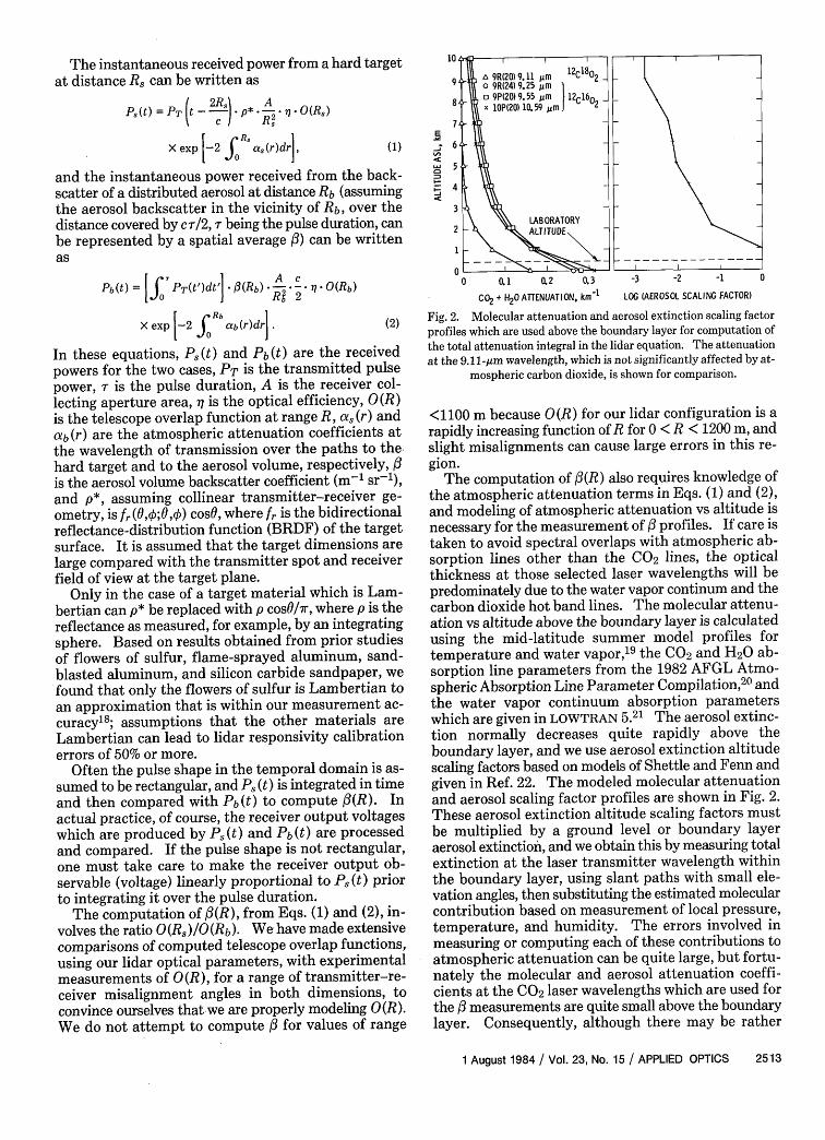
Fig. 2. Molecular attenuation and aerosol extinction scaling factor

profiles which are used above the boundary layer for computation of

the total attenuation integral in the lidar equation. The attenuationat the 9.11-Am wavelength, which is not significantly affected by at-

mospheric carbon dioxide, is shown for comparison.

<1100 m because O(R) for our lidar configuration is arapidly increasing function of R for 0 < R < 1200 m, andslight misalignments can cause large errors in this re-gion.

The computation of $(R) also requires knowledge ofthe atmospheric attenuation terms in Eqs. (1) and (2),and modeling of atmospheric attenuation vs altitude isnecessary for the measurement of / profiles. If care istaken to avoid spectral overlaps with atmospheric ab-sorption lines other than the CO2 lines, the opticalthickness at those selected laser wavelengths will bepredominately due to the water vapor continum and thecarbon dioxide hot band lines. The molecular attenu-ation vs altitude above the boundary layer is calculatedusing the mid-latitude summer model profiles fortemperature and water vapor,19 the CO2 and H20 ab-sorption line parameters from the 1982 AFGL Atmo-spheric Absorption Line Parameter Compilation,2 0 andthe water vapor continuum absorption parameterswhich are given in LOWTRAN 5.21 The aerosol extinc-tion normally decreases quite rapidly above theboundary layer, and we use aerosol extinction altitudescaling factors based on models of Shettle and Fenn andgiven in Ref. 22. The modeled molecular attenuationand aerosol scaling factor profiles are shown in Fig. 2.These aerosol extinction altitude scaling factors mustbe multiplied by a ground level or boundary layeraerosol extinction, and we obtain this by measuring totalextinction at the laser transmitter wavelength withinthe boundary layer, using slant paths with small ele-vation angles, then substituting the estimated molecularcontribution based on measurement of local pressure,temperature, and humidity. The errors involved inmeasuring or computing each of these contributions toatmospheric attenuation can be quite large, but fortu-nately the molecular and aerosol attenuation coeffi-cients at the CO2 laser wavelengths which are used forthe / measurements are quite small above the boundarylayer. Consequently, although there may be rather

1 August 1984 / Vol. 23, No. 15 / APPLIED OPTICS 2513

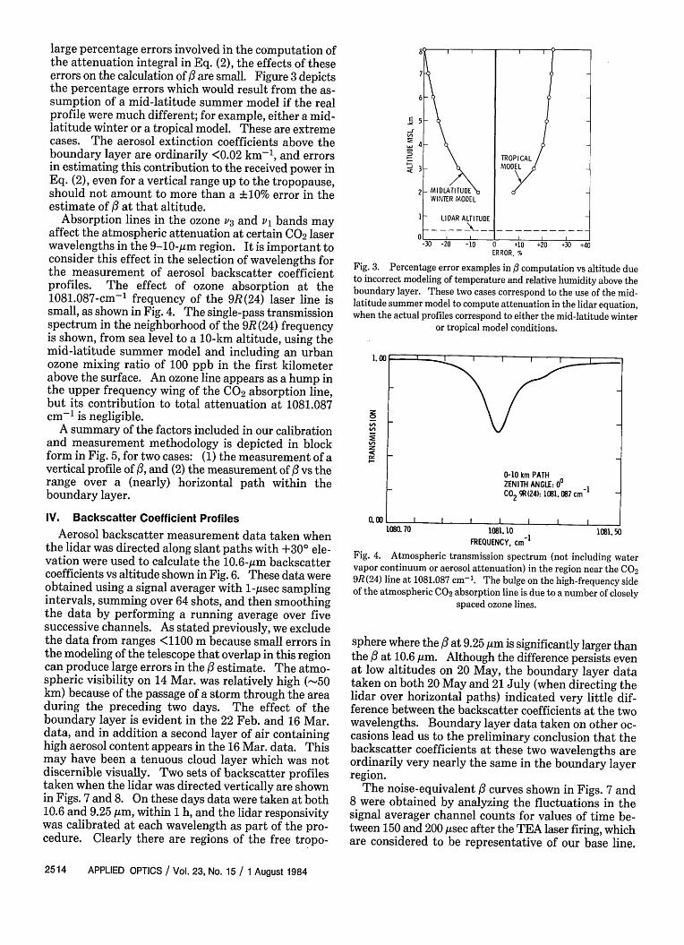
large percentage errors involved in the computation ofthe attenuation integral in Eq. (2), the effects of theseerrors on the calculation of fl are small. Figure 3 depictsthe percentage errors which would result from the as-sumption of a mid-latitude summer model if the realprofile were much different; for example, either a mid-latitude winter or a tropical model. These are extremecases. The aerosol extinction coefficients above theboundary layer are ordinarily <0.02 km-', and errorsin estimating this contribution to the received power inEq. (2), even for a vertical range up to the tropopause,should not amount to more than a 10% error in theestimate of /3 at that altitude.

Absorption lines in the ozone 3 and vi bands mayaffect the atmospheric attenuation at certain CO2 laserwavelengths in the 9 -10 -ym region. It is important toconsider this effect in the selection of wavelengths forthe measurement of aerosol backscatter coefficientprofiles. The effect of ozone absorption at the1081.087-cm-1 frequency of the 9R(24) laser line issmall, as shown in Fig. 4. The single-pass transmissionspectrum in the neighborhood of the 9R(24) frequencyis shown, from sea level to a 10-km altitude, using themid-latitude summer model and including an urbanozone mixing ratio of 100 ppb in the first kilometerabove the surface. An ozone line appears as a hump inthe upper frequency wing of the CO2 absorption line,but its contribution to total attenuation at 1081.087cm-1 is negligible.

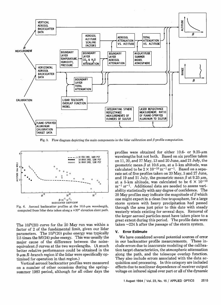
A summary of the factors included in our calibrationand measurement methodology is depicted in blockform in Fig. 5, for two cases: (1) the measurement of avertical profile of , and (2) the measurement of /3 vs therange over a (nearly) horizontal path within theboundary layer.

IV. Backscatter Coefficient Profiles

Aerosol backscatter measurement data taken whenthe lidar was directed along slant paths with +30° ele-vation were used to calculate the 10.6-Atm backscattercoefficients vs altitude shown in Fig. 6. These data wereobtained using a signal averager with 1-Atsec samplingintervals, summing over 64 shots, and then smoothingthe data by performing a running average over fivesuccessive channels. As stated previously, we excludethe data from ranges <1100 m because small errors inthe modeling of the telescope that overlap in this regioncan produce large errors in the /3 estimate. The atmo-spheric visibility on 14 Mar. was relatively high (50km) because of the passage of a storm through the areaduring the preceding two days. The effect of theboundary layer is evident in the 22 Feb. and 16 Mar.data, and in addition a second layer of air containinghigh aerosol content appears in the 16 Mar. data. Thismay have been a tenuous cloud layer which was notdiscernible visually. Two sets of backscatter profilestaken when the lidar was directed vertically are shownin Figs. 7 and 8. On these days data were taken at both10.6 and 9.25 m, within 1 h, and the lidar responsivitywas calibrated at each wavelength as part of the pro-cedure. Clearly there are regions of the free tropo-

-f

4 -4

,4TROPICAL. 3 MODEL

2 MI DLATITUDEWINTER MODEL

1 LIDAR ALTITUDE

-30 -20 -10 0 +10 +20 +30 +40ERROR, %

Fig. 3. Percentage error examples in ,B computation vs altitude dueto incorrect modeling of temperature and relative humidity above theboundary layer. These two cases correspond to the use of the mid-latitude summer model to compute attenuation in the lidar equation,when the actual profiles correspond to either the mid-latitude winter

or tropical model conditions.

1.

-

W

0.001080. 70 1081.10 1081. 50

FREQUENCY, cm

Fig. 4. Atmospheric transmission spectrum (not including watervapor continuum or aerosol attenuation) in the region near the CO29R(24) line at 1081.087 cm-1. The bulge on the high-frequency sideof the atmospheric CO2 absorption line is due to a number of closely

spaced ozone lines.

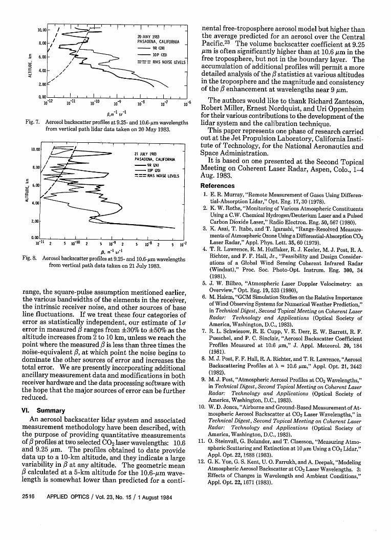
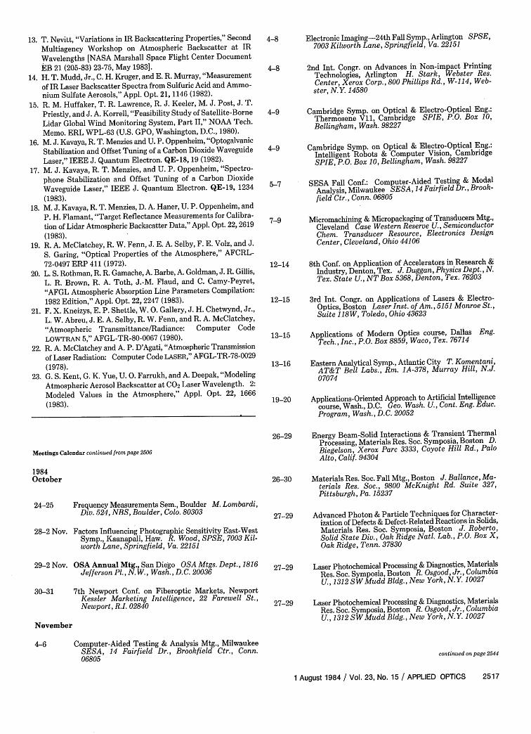
sphere where the /3 at 9.25 um is significantly larger thanthe /3 at 10.6 m. Although the difference persists evenat low altitudes on 20 May, the boundary layer datataken on both 20 May and 21 July (when directing thelidar over horizontal paths) indicated very little dif-ference between the backscatter coefficients at the twowavelengths. Boundary layer data taken on other oc-casions lead us to the preliminary conclusion that thebackscatter coefficients at these two wavelengths areordinarily very nearly the same in the boundary layerregion.

The noise-equivalent 13 curves shown in Figs. 7 and8 were obtained by analyzing the fluctuations in thesignal averager channel counts for values of time be-tween 150 and 200 sec after the TEA laser firing, whichare considered to be representative of our base line.

2514 APPLIED OPTICS / Vol. 23, No. 15 / 1 August 1984

MEASUREMENT

CALI BRATION

Fig. 5. Flow diagram depicting the main components in the lidar calibration and : profile computation.

Z

lo- 10-7

13( 1 sr )BACKSCATTER COEFFICIENT

Fig. 6. Aerosol backscatter profiles at the 10.6-jim wavelength,computed from lidar data taken along a +30° elevation slant path.

The 1OP(20) curve for the 20 May run was within afactor of 2 of the fundamental limit, given our lidarparameters. The 1OP(20) pulse energy was typically2.5 times the 9R (24) pulse energy. This was usually themajor cause of the difference between the noise-equivalent / curves at the two wavelengths. (A muchbetter relative performance could be obtained in the9-Atm R -branch region if the lidar were specifically op-timized for operation in that region.)

Vertical aerosol backscatter profiles were measuredon a number of other occasions during the spring-summer 1983 period, although for all other days the

profiles were obtained for either 10.6- or 9.25-Atmwavelengths but not both. Based on six profiles takenon 11,20, and 27 May, 13 and 20 June, and 21 July, thegeometric mean /3 at 10.6 Am, at a 5-km altitude, wascalculated to be 2 X 10-10 m- 1 sr-1 . Based on a sepa-rate set of five profiles taken on 20 May, 3 and 27 June,and 19 and 21 July, the geometric mean / at 9.25 Am,at a 5-km altitude, was calculated to be 6 X 10-10m-1 sr-'. Additional data are needed to assess vari-ability statistically with any degree of confidence. The20 May profiles may indicate the magnitude of / whichone might expect in a clean free troposphere, for a largestorm system with heavy precipitation had passedthrough the area just prior to this date with steadywesterly winds existing for several days. Removal ofthe larger aerosol particles must have taken place to agreat extent during this period. The profile data weretaken -224 h after the passage of the storm system.

V. Error Estimate

We have considered several potential sources of errorin our backscatter profile measurements. These in-clude errors due to inaccurate modeling of the calibra-tion target characteristics, the atmospheric attenuationalong the path, and the telescope overlap function.They also include errors associated with the data ac-quisition and processing. In this category are includedeffects due to nonlinear dependence of receiver outputvoltage on infrared signal over part or all of the dynamic

1 August 1984 / Vol. 23, No. 15 / APPLIED OPTICS 2515

-_ _,o 22 FEB 1983, 1600 PST@0000 14 MAR 1983, 1200 PST00000 16 MAR 1983, 1100 PST

04*

0 0 00°

' I ' ' I ' ' ' I , , I

6

2

10-8

E 6.00 _ - Fti (M)/ , < = === RMS NOISE LEVELS

: 4.00 /

2.00

Q00 ' ' f | @ | [, I,, I,,~~C I I,10 12 lo-II lo-lo 10-9 10-8 10 10 l1-

,m sr 1

Fig. 7. Aerosol backscatter profiles at 9.25- and 10.6-jim wavelengthsfrom vertical path lidar data taken on 20 May 1983.

10.00 21 JULY 1983

PASADENA. CALFORNI8 / R 12418.00 U- O (201

==RMS NOISE LEVELSE

.6.0 OD

4.00

lo-II 2 5 io '1 2 5 10 9 2 5 108 2 5 10

, M-' sr-'Fig. 8. Aerosol backscatter profiles at 9.25- and 10.6-,m wavelengths

from vertical path data taken on 21 July 1983.

range, the square-pulse assumption mentioned earlier,the various bandwidths of the elements in the receiver,the intrinsic receiver noise, and other sources of baseline fluctuations. If we treat these four categories oferror as statistically independent, our estimate of 1error in measured ranges from 30% to ±50% as thealtitude increases from 2 to 10 km, unless we reach thepoint where the measured is less than three times thenoise-equivalent 13, at which point the noise begins todominate the other sources of error and increases thetotal error. We are presently incorporating additionalancillary measurement data and modifications in bothreceiver hardware and the data processing software withthe hope that the major sources of error can be furtherreduced.

VI. Summary

An aerosol backscatter lidar system and associatedmeasurement methodology have been described, withthe purpose of providing quantitative measurementsof profiles at two selected CO2 laser wavelengths: 10.6and 9.25 Am. The profiles obtained to date providedata up to a 10-km altitude, and they indicate a largevariability in 13 at any altitude. The geometric mean/ calculated at a 5-km altitude for the 10.6-Atm wave-length is somewhat lower than predicted for a conti-

nental free-troposphere aerosol model but higher thanthe average predicted for an aerosol over the CentralPacific.23 The volume backscatter coefficient at 9.25gtm is often significantly higher than at 10.6 Am in thefree troposphere, but not in the boundary layer. Theaccumulation of additional profiles will permit a moredetailed analysis of the /3 statistics at various altitudesin the troposphere and the magnitude and consistencyof the enhancement at wavelengths near 9 Atm.

The authors would like to thank Richard Zanteson,Robert Miller, Ernest Nordquist, and Uri Oppenheimfor their various contributions to the development of thelidar system and the calibration technique.

This paper represents one phase of research carriedout at the Jet Propulsion Laboratory, California Insti-tute of Technology, for the National Aeronautics andSpace Administration.

It is based on one presented at the Second TopicalMeeting on Coherent Laser Radar, Aspen, Colo., 1-4Aug. 1983.

References1. E. R. Murray, "Remote Measurement of Gases Using Differen-

tial-Absorption Lidar," Opt. Eng. 17, 30 (1978).2. K. W. Rothe, "Monitoring of Various Atmospheric Constituents

Using a C.W. Chemical Hydrogen/Deuterium Laser and a PulsedCarbon Dioxide Laser," Radio Electron. Eng. 50, 567 (1980).

3. K. Asai, T. Itabe, and T. Igarashi, "Range-Resolved Measure-ments of Atmospheric Ozone Using a Differential-Absorption CO2Laser Radar," Appl. Phys. Lett. 35, 60 (1979).

4. T. R. Lawrence, R. M. Huffaker, R. J. Keeler, M. J. Post, R. A.Richter, and F. F. Hall, Jr., "Feasibility and Design Consider-ations of a Global Wind Sensing Coherent Infrared Radar(Windsat)," Proc. Soc. Photo-Opt. Instrum. Eng. 300, 34(1981).

5. J. W. Bilbro, "Atmospheric Laser Doppler Velocimetry: anOverview," Opt. Eng. 19, 533 (1980),

6. M. Halem, "GCM Simulation Studies on the Relative Importanceof Wind Observing Systems for Numerical Weather Prediction,"in Technical Digest, Second Topical Meeting on Coherent LaserRadar: Technology and Applications (Optical Society ofAmerica, Washington, D.C., 1983).

7. R. L. Schwiesow, R. E. Cupp, V. E. Derr, E. W. Barrett, R. F.Pueschel, and P. C. Sinclair, "Aerosol Backscatter CoefficientProfiles Measured at 10.6 im," J. Appl. Meteorol. 20, 184(1981).

8. M. J. Post, F. F. Hall, R. A. Richter, and T. R. Lawrence, "AerosolBackscattering Profiles at X = 10.6 ,m," Appl. Opt. 21, 2442(1982).

9. M. J. Post, "Atmospheric Aerosol Profiles at CO2 Wavelengths,"in Technical Digest, Second Topical Meeting on Coherent LaserRadar: Technology and Applications (Optical Society ofAmerica, Washington, D.C., 1983).

10. W. D. Jones, "Airborne and Ground-Based Measurement of At-mospheric Aerosol Backscatter at CO2 Laser Wavelengths," inTechnical Digest, Second Topical Meeting on Coherent LaserRadar: Technology and Applications (Optical Society ofAmerica, Washington, D.C., 1983).

11. 0. Steinvall, G. Bolander, and T. Claesson, "Measuring Atmo-spheric Scattering and Extinction at 10 m Using a CO2 Lidar,"Appl. Opt. 22, 1688 (1983).

12. G. K. Yue, G. S. Kent, U. 0. Farrukh, and A. Deepak, "ModelingAtmospheric Aerosol Backscatter at CO2 Laser Wavelengths. 3:Effects of Changes in Wavelength and Ambient Conditions,"Appl. Opt. 22, 1671 (1983).

2516 APPLIED OPTICS / Vol. 23, No. 15 / 1 August 1984

13. T. Nevitt, "Variations in IR Backscattering Properties," Second

Multiagency Workshop on Atmospheric Backscatter at IR

Wavelengths [NASA Marshall Space Flight Center DocumentEB 21 (205-83) 23-75, May 1983].

14. H. T. Mudd, Jr., C. H. Kruger, and E. R. Murray, "Measurement

of IR Laser Backscatter Spectra from Sulfuric Acid and Ammo-nium Sulfate Aerosols," Appl. Opt. 21, 1146 (1982).

15. R. M. Huffaker, T. R. Lawrence, R. J. Keeler, M. J. Post, J. T.

Priestly, and J. A. Korrell, "Feasibility Study of Satellite-BorneLidar Global Wind Monitoring System, Part II," NOAA Tech.Memo. ERL WPL-63 (U.S. GPO, Washington, D.C., 1980).

16. M. J. Kavaya, R. T. Menzies and U. P. Oppenheim, "Optogalvanic

Stabilization and Offset Tuning of a Carbon Dioxide Waveguide

Laser," IEEE J. Quantum Electron. QE-18, 19 (1982).17. M. J. Kavaya, R. T. Menzies, and U. P. Oppenheim, "Spectro-

phone Stabilization and Offset Tuning of a Carbon Dioxide

Waveguide Laser," IEEE J. Quantum Electron. QE-19, 1234(1983).

18. M. J. Kavaya, R. T. Menzies, D. A. Haner, U. P. Oppenheim, and

P. H. Flamant, "Target Reflectance Measurements for Calibra-tion of Lidar Atmospheric Backscatter Data," Appl. Opt. 22, 2619

(1983).19. R. A. McClatchey, R. W. Fenn, J. E. A. Selby, F. E. Volz, and J.

S. Garing, "Optical Properties of the Atmosphere," AFCRL-72-0497 ERP 411 (1972).

20. L. S. Rothman, R. R. Gamache, A. Barbe, A. Goldman, J. R. Gillis,

L. R. Brown, R. A. Toth, J.-M. Flaud, and C. Camy-Peyret,

"AFGL Atmospheric Absorption Line Parameters Compilation:

1982 Edition," Appl. Opt. 22, 2247 (1983).

21. F. X. Kneizys, E. P. Shettle, W. 0. Gallery, J. H. Chetwynd, Jr.,

L. W. Abreu, J. E. A. Selby, R. W. Fenn, and R. A. McClatchey,

"Atmospheric Transmittance/Radiance: Computer CodeLOWTRAN 5," AFGL-TR-80-0067 (1980).

22. R. A. McClatchey and A. P. D'Agati, "Atmospheric Transmission

of Laser Radiation: Computer Code LASER," AFGL-TR-78-0029

(1978).23. G. S. Kent, G. K. Yue, U. 0. Farrukh, and A. Deepak, "Modeling

Atmospheric Aerosol Backscatter at CO2 Laser Wavelength. 2:

Modeled Values in the Atmosphere," Appl. Opt. 22, 1666

(1983).

4-8 Electronic Imaging-24th Fall Symp., Arlington SPSE,7003 Kilworth Lane, Springfield, Va. 22151

4-8 2nd Int. Congr. on Advances in Non-impact PrintingTechnologies, Arlington H. Stark, Webster Res.Center, Xerox Corp., 800 Phillips Rd., W-114, Web-ster, N.Y. 14580

4-9 Cambridge Symp. on Optical & Electro-Optical Eng.:Thermosene V11, Cambridge SPIE, P.O. Box 10,Bellingham, Wash. 98227

4-9 Cambridge Symp. on Optical & Electro-Optical Eng.:Intelligent Robots & Computer Vision, CambridgeSPIE, P.O. Box 10, Bellingham, Wash. 98227

5-7 SESA Fall Conf.: Computer-Aided Testing & ModalAnalysis, Milwaukee SESA, 14 Fairfield Dr., Brook-field Ctr., Conn. 06805

7-9 Micromachining & Micropackaging of Transducers Mtg.,Cleveland Case Western Reserve U., SemiconductorChem. Transducer Resource, Electronics DesignCenter, Cleveland, Ohio 44106

12-14 8th Conf. on Application of Accelerators in Research &Industry, Denton, Tex. J. Duggan, Physics Dept., N.Tex. State U., NT Box 5368, Denton, Tex. 76203

12-15 3rd Int. Congr. on Applications of Lasers & Electro-Optics, Boston Laser Inst. of Am., 5151 Monroe St.,Suite 118W, Toledo, Ohio 43623

13-15 Applications of Modern Optics course, Dallas Eng.Tech., Inc., P.O. Box 8859, Waco, Tex. 76714

13-16 Eastern Analytical Symp., Atlantic City T. Komentani,AT&T Bell Labs., Rm. 1A-378, Murray Hill, N.J.07074

19-20 Applications-Oriented Approach to Artificial Intelligencecourse, Wash., D.C. Geo. Wash. U., Cont. Eng. Educ.

Program, Wash., D.C. 20052

Meetings Calendar continued from page 2506

1984October

24-25 Frequency Measurements Sem., Boulder M. Lombardi,Div. 524, NBS, Boulder, Colo. 80303

28-2 Nov. Factors Influencing Photographic Sensitivity East-WestSymp., Kaanapali, Haw. R. Wood, SPSE, 7003 Kil-worth Lane, Springfield, Va. 22151

29-2 Nov. OSA Annual Mtg., San Diego OSA Mtgs. Dept., 1816Jefferson P1., N. W., Wash., D.C. 20036

30-31 7th Newport Conf. on Fiberoptic Markets, NewportKessler Marketing Intelligence, 22 Farewell St.,Newport, R.I. 02840

November

26-29 Energy Beam-Solid Interactions & Transient ThermalProcessing, Materials Res. Soc. Symposia, Boston D.Biegelson, Xerox Parc 3333, Coyote Hill Rd., PaloAlto, Calif. 94304

26-30 Materials Res. Soc. Fall Mtg., Boston J. Ballance, Ma-terials Res. Soc., 9800 McKnight Rd. Suite 327,Pittsburgh, Pa. 15237

27-29 Advanced Photon & Particle Techniques for Character-ization of Defects & Defect-Related Reactions in Solids,Materials Res. Soc. Symposia, Boston J. Roberto,Solid State Div., Oak Ridge Natl. Lab., P.O. Box X,Oak Ridge, Tenn. 37830

27-29 Laser Photochemical Processing & Diagnostics, MaterialsRes. Soc. Symposia, Boston R. Osgood, Jr., ColumbiaU., 1312 SWMudd Bldg., New York, N.Y. 10027

27-29 Laser Photochemical Processing & Diagnostics, MaterialsRes. Soc. Symposia, Boston R. Osgood, Jr., ColumbiaU., 1312 SW Mudd Bldg., New York, N. Y. 10027

4-6 Computer-Aided Testing & Analysis Mtg., MilwaukeeSESA, 14 Fairfield Dr., Brookfield Ctr., Conn.06805

continued on page 2544

1 August 1984 / Vol. 23, No. 15 / APPLIED OPTICS 2517