atlantic decadal variability:combining observations and ... · pdf fileukgs ingv mri-eccosio...

National Oceanic and Atmospheric AdministrationGeophysical Fluid Dynamics Laboratory

Princeton, NJ 08542http://www.gfdl.noaa.gov

Atlantic Decadal Variability:Combining observations and models to investigate predictability

A.Rosati NOAA/GFDL

With T.Delworth, S. Zhang

Understanding Ocean-Atmosphere Interactions in the Tropical Pacific has Laid the Foundations for Physics –

Based Seasonal Forecasts

Evolution of El Nino and La Nina

The close interplay between hypotheses, successes in confronting

theories and observations, and observed (and attributable) impacts were factor in this success.

In contrast to S/I forecasting decadal climate predictions are in their infancy.

OUTLINE• Decadal Variability• Atlantic Multi-decadal Oscillation (AMO)• Meridional Overturning Circulation (MOC)

and AMO• Predictability of MOC• Current Status of Ocean Data Assimilation

(ODA) from CLIVAR GSOP• Can we Constrain the MOC with the current

ocean observing system? - Perfect Model Assimilation Studies

• Summary of Atlantic Variability Workshops

Some Regional Decadal Predictability is Associated with Global Warming

Model forced with observed SSTs Specified radiative forcing from 1860

Ocean specified - land predicted Ocean and Land predicted, but missing impacts of natural decadal variability

Understanding Both Natural Climate Variability and Global Warming is Critical for Attribution Studies

Global decadal climate variability underlies much of these variationsWhat are the common mechanisms linking droughts, hurricanes, fisheries?

National Oceanic and Atmospheric AdministrationGeophysical Fluid Dynamics Laboratory

Princeton, NJ 08542http://www.gfdl.noaa.gov

How Well Do We Understand the Climate of the 20th

Century?

+ =

trends

Multidecadal signals

Observations?

Successful Simulations? Or is the explanation more complicated?

More strong hurricanes

Drought

More rain over Saheland western India

Warm North Atlantic linked to …

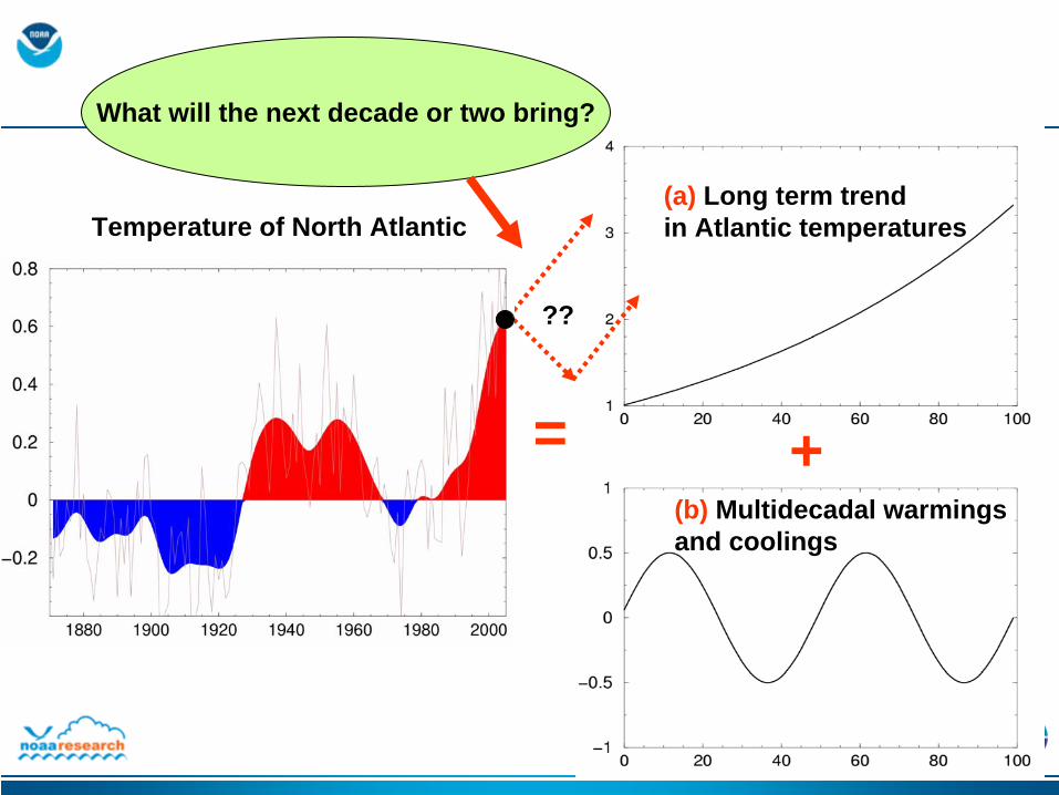
Two important aspects:a. Decadal-multidecadal fluctuationsb. Long-term trend

Atlantic Meridional Overturning Circulation

(AMOC)

North Atlantic Temperature

+=

(a) Long term trendin Atlantic temperatures

(b) Multidecadal warmingsand coolings

Temperature of North Atlantic

??

What will the next decade or two bring?

As climate warms,Atlantic ocean circulation weakens

Strength of ocean circulation

Modelprojection

Putting the pieces together …

1. Decadal-multidecadal fluctuationsa. Natural variabilityb. Forced change

2. Long-term weakening trend of circulation

GOAL: Predict decadal scale evolution of the Atlantic in response to multiple factors

Decadal Variability is a Major Factor in Atlantic During the 20th

Century

Sea Surface Temperature (SST) Differences1941-1960 minus 1965-1984

Average North Atlantic Temperatures with trend removed

This variation is termed the Atlantic Multi-Decadal Oscillation (AMO)

Simulated SST anomaly from the water-hosing experiment (Zhang and Delworth 2005)

Observed SST Difference (1971-1990) – (1941-1960) (HadISST, detrended)

Atlantic Changes (Decadal and Longer) Have Global Impacts

What is the Potential for Abrupt Changes in the Near Future?

Global temperature changes resulting from an Atlantic THC shut down

Models suggest a slow down of the Atlantic thermohaline circulation (THC) in the 21st

C

Note: the aerosol effects have delayed the onset of this

Model Description: GFDL CM2.1 - Latest developed fully coupled GCM (Delworth et al., 2005)

To simulate the impact of AMO, we modified CM2.1 into a hybrid coupled model: the Atlantic basin is modified to a slab ocean, all other are the same as CM2.1 (Zhang and Delworth 2006)

Schematic diagram of the hybrid coupled model Observed AMO Index (HadISST)

10-member ensemble experiments: forced by the same anomalous qflux in the Atlantic modulated by observed AMO Index (1901-2000)

Rong Zhang Tom Delworth

Impact of the Atlantic Multidecadal Oscillation on the 20th Century Climate Variability

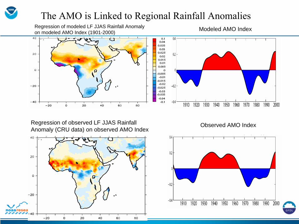
Regression of modeled LF JJAS Rainfall Anomaly on modeled AMO Index (1901-2000) Modeled AMO Index

Regression of observed LF JJAS Rainfall Anomaly (CRU data) on observed AMO Index

Observed AMO Index

The AMO is Linked to Regional Rainfall Anomalies

Impact of AMO on Atlantic Hurricane Activity

NOAA 2005 Atlantic Hurricane Outlook

ECMWF 40-yr Reanalysis

Regression of LF ASO vertical shear of zonal wind (m/s) on AMO index (1958-2000)

MODEL (10-member ensemble mean)

The AMO Has Played an Important Role During the 20th

Century in Decadal Modulation of Hurricane Activity

Studies, which are currently under way to study the decadal predictability of the AMO, show some promise

What is the Origin of the Decadal Variability in Northern Hemisphere Temperatures?

(Blue: Observed temperatures with the linear 100 yr trend removed)

Red: ensemble mean temperature where the Atlantic is forced with anomalous heat flux that approximates AMO

Red: ensemble mean when model forced with radiative forcing with linear trend removed

Is there a link between radiative forcings and Atlantic decadal variability??

Mechanisms of AMO

The AMO is thought to be driven by multidecadal variability of the Atlantic thermohaline circulation (THC)

(Bjerknes 1964; Folland 1984; Delworth et al., 1993; Delworth and Mann 2000; Latif et al 2004)

Enhanced THC strength enhances the poleward transport of heat in the North Atlantic, driving the large- scale positive SST anomalies.

Changes in vertical and horizontal density gradients in the North Atlantic alter the THC (enhanced density gradients strengthen the THC)

How will the Atlantic change in the future?

Two primary influences:

1. Natural variability of the Atlantic (AMO)From known initial state, use modelsto predict the decadal-scale evolution of the system.

2. Response to anthropogenic forcinga. Direct thermal responseb. Ocean circulation response (thermohaline circulation)c. Other factors (Atmospheric circulation changes;

Greenland ice sheet; etc.)

Projected Atlantic Sea Surface Temperature Change(relative to 1991-2004 mean)

Areal average70oW-0oW0oN-60oN

Results from GFDL CM2.1- sres A1B

ObservedTrend from 1950-2004

ObservedChange

2001-2004Minus1965-1984

Projected Change

2041-2050Minus2001-2005

Summary

1. The Atlantic Multidecadal Oscillation (AMO) is a prominent mode of Atlantic variability with significant climate links (hurricanes, rainfall, temperature)

2. Observed Atlantic behavior is a combination of the AMO and a long term warming trend, with the trend likely a response to increasing greenhouse gases.


variability in CGCMs• Predictability of MOC• Current Status of Ocean Data Assimilation

(ODA)• Can we Constrain the MOC with the current



CM2.1 MOC wavelet analysis

From A. Wittenberg

MOC in Present-Day Control Experiments from G. Danabasoglu,NCAR

CCSM3-T85x1

CCSM3-T42x1

CCSM2-T42x1

CCSM3-T31x3

CCSM2.2-T42x1

QUESTIONS: Atlantic Decadal Variability Workshop G. Danabasoglu,NCAR

•

What are the dynamical mechanisms of the decadal oscillations of

the MOC?•

How does this oscillation affect our assessment of 20th

century, future scenario, etc. climates?

•

What are the effects on predictability?•

How do we initialize our ensemble integrations with this oscillation present?

“What are the pros and cons of initial ocean states for climate change scenario ensemble integrations with the same vs. different phases of the MOC or other oceanic oscillatory phenomena, and how would that relate to the number of ensemble members required for analysis?”

A discussion topic at the 11th

Annual CCSM Workshop

•

Why does it appear to depend on model resolution?•

Does the amplitude of the oscillation depend on the mean state?•

What are the regional and global impacts of the variability?

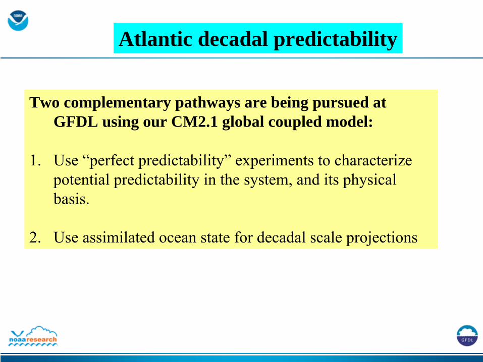
Atlantic decadal predictability

Two complementary pathways are being pursued at GFDL using our CM2.1 global coupled model:

1.

Use “perfect predictability”

experiments to characterizepotential predictability in the system, and its physical basis.

2. Use assimilated ocean state for decadal scale projections

The

N. A

tl. M

OC

in th

e 18

60 C

ontro

l

Decadal Variability is Present in GFDL’s

Models –

This Enables Decadal Predictability Studies

Decadal Predictability Experimental Design

Our investigation begins by arbitrarily selecting 6 points in time from the long control experiment.

The 6 “initialization points” are separated by 100 years. (1 Jan 1001, 1101, 1201, 1301, 1401 & 1501)

We first focus on the annual mean N. Atlantic MOC strength for the 20 year periods beginning at each of the 6 initialization points. So, they are…

1001-1020 1301-1320 1101-1120 1401-14201201-1220 1501-1520

The

N. A

tl. M

OC

in th

e 18

60 C

ontro

l

Preliminary Experimental DesignBuilding some small ensembles:The CM2.1 model produces a separate restart file for each of its 4 main subcomponents.

In our first line of inquiry, we generated ensembles of 20 year long runs by mixing atmospheric restarts drawn from days >5 days and < 1 month from the 1 Jan initialization used for the ocean, land & sea ice restarts. For example…

Building some small ensembles:The CM2.1 model produces a separate restart file for each of its 4 main subcomponents.

In our first line of inquiry, we generated ensembles of 20 year long runs by mixing atmospheric restarts drawn from days >5 days and < 1 month from the 1 Jan initialization used for the ocean, land & sea ice restarts. For example…

sea ice atmosocean land

Preliminary Experimental Design

1 Jan 1001 06 Jan 100111 Jan 100116 Jan 100121 Jan 100126 Jan 1001

generating a ten member ensemble

07 Dec 100012 Dec 100017 Dec 100022 Dec 100027 Dec 1000

?? Will the ensemble members suggest Atl. MOC exists over periods of a decade or longer…

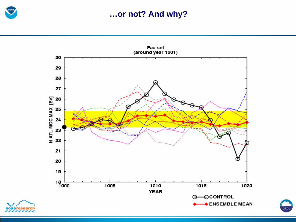
…or not? And why?

“The MM ensemble indicates considerable predictability in the N.A. MOC variations on dacadal time scales.”

(Collins et al. 2006)

Latif et al. (2004)

•

Decadal prediction is not only an initial value problem but also a boundary value problem.

•Anthropogenic effects need to be taken into account for longterm

forecasts.

•Much of the prediction results depend on a proper initialization. ODA still not mature.



(ODA) from CLIVAR GSOP• Can we Constrain the MOC with the current



Sampling

Uncertainty in the Mean

24m-rm EQPAC Averaged temperature over the top 300m

1950 1960 1970 1980 1990 2000Time

16

17

18

19

20

21

ukdpukoicfcs2cfas2ecco50y

gfdlsodaecmfaecmfcukgs

ingvmri-eccoSIOcfasamct2

mct3eccoJPLaeccoJPLceccoMITGMAO

sdv ensm = 0.260s/n ensm = 0.544

sdv all = 0.448s/n all = 0.939

spread = 0.478

•Ambiguity in the definitionclosest level, interpolated values…?

•Real Uncertainty?

Forcing fluxes and analysis methods are largest source of uncertainty

Data Assimilation does not always collapse the spread: We need to pay more attention to the assimilation methods.

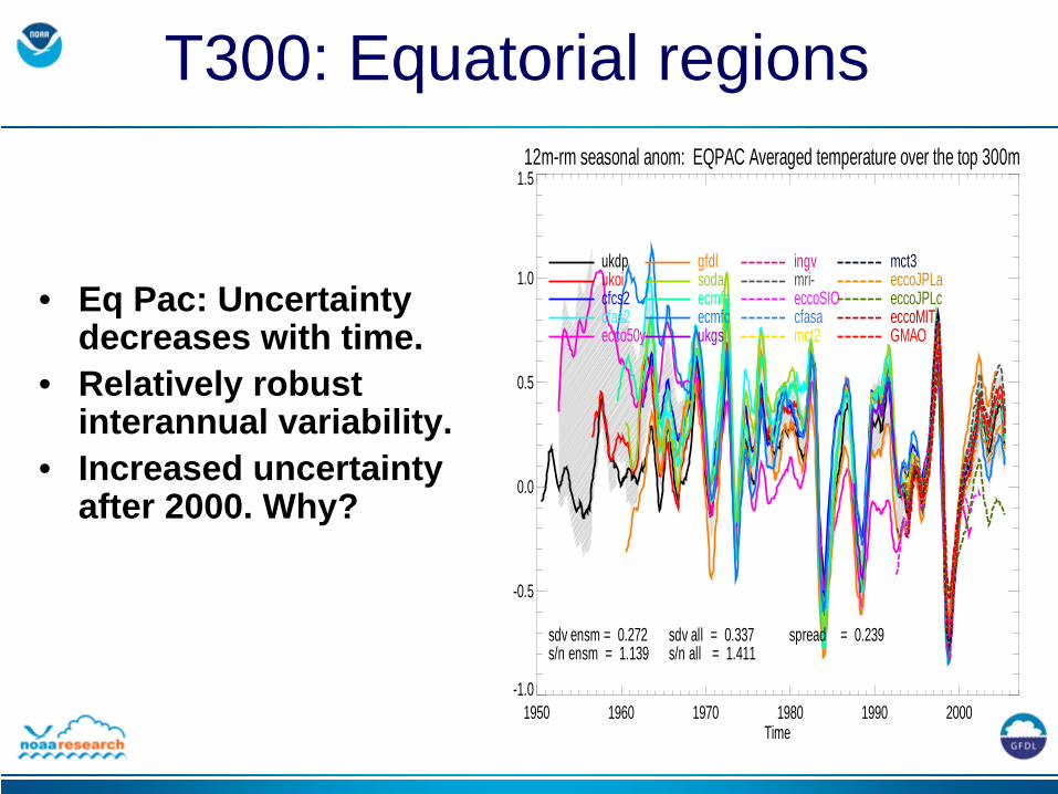
T300: Equatorial regions

• Eq Pac: Uncertainty decreases with time.

• Relatively robust interannual variability.

• Increased uncertainty after 2000. Why?

12m-rm seasonal anom: EQPAC Averaged temperature over the top 300m

1950 1960 1970 1980 1990 2000Time

-1.0

-0.5

0.0

0.5

1.0

1.5






sdv all = 0.337s/n all = 1.411

spread = 0.239

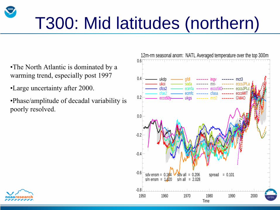
T300: Mid latitudes (northern)12m-rm seasonal anom: NATL Averaged temperature over the top 300m

1950 1960 1970 1980 1990 2000Time

-0.8

-0.6

-0.4

-0.2

0.0

0.2

0.4

0.6






sdv all = 0.206s/n all = 2.028

spread = 0.101

•The North Atlantic is dominated by a warming trend, especially post 1997

•Large uncertainty after 2000.

•Phase/amplitude of decadal variability is poorly resolved.

Summary

• sampling issues (even for the 90’s period)

•

significant differences between data fits (normalized)

•

most probably room for better model-data fit (without over-fitting)

Transport Measures0

( , , ) ( , , , )xe

z xwy z t V x y z t dxdzψ = ∫ ∫

0( , ) ( , , , ) ( , , , )

xe

H xwHT y t V x y z t T x y z t dxdz

−= ⋅∫ ∫

35 ,)/),,,(1(),,,(),(0

=−⋅= ∫ ∫−o

H

xe

xwo SdxdzStzyxStzyxVtyST

Meridional overturning, MOC:

Heat transport (rel. 0oC):

Freshwater transport (rel. 35 psu):

Heat transport 25oN

Heat transport 48oN

Max. MOC 25oN

Bryden et al. (2005)

ECMWF

Max. MOC 48oN

Atlantic MOCECCO-SIO

ECCO-50y

ECCO-GODAE

ECCO-JPL

INGV

SODA

GFDL

Heat/FW transport

Heat/FW transport

Global Mean 25N (PW)

Global Mean 20S (PW)

Ind.- Pac. Mean 25N (PW)

Atl. Mean 25N (PW)

Atl. STD 25N (PW)

Atl. Seasonal 25N (PW)

Atl. Drift 25N (PW/10y r)

Global Mean FW 30S (Sv)

Global Mean FW 25N (Sv)

Model Details

Method Details

Ganachaud& Wunsch (2000)

1.80 -0.80 0.50 1.30 Macdonald (1998) 0.72 -0.3

ECCO-JPL 1.45 -1.30 0.44 1.01 0.30 -0.37 0.50 -0.35 MIT 1-1/3o, Lev KPP, GM

partition Kalman

ECCO-SIO 1.40 -0.44 0.45 0.96 0.21 0.13 -0.08 0.35 -0.31 MIT 1o, Lev, KPP, GM

adjoint

ECCO-50yr 1.26 -0.63 0.38 0.88 0.21 0.14 0.034 0.33 -0.31 MIT 1o,Lev, KPP, GM

adjoint

ECCO- GODAE

1.15 -0.78 0.33 0.82 0.21 0.13 0.033 0.55 -0.31 MIT 1o,Lev adjoint

GFDL 1.01 0.22 0.20 0.77 0.31 0.11 -0.018 MOM 3D-var

INGV 2.2 -1.1 0.7 1.45 0.25 0.11 -0.27 0.82 -0.45 OPA 2- 1/2o,Lev, TKE, eddy vel

multivar. OI

SODA 0.99 0.16 -0.08 MOM 1-1/3o

Lev KPP,GMOI

Questions

• Why is the spread so large between reanalysis?

• relationships between observed and unobserved quantities.

• quality/uncertainties of climatological means.

• impact on the fit to observations of:a) model constraints (strong? weak?), assimilation window length b) weightingc) methodology in general

• data sets used for comparison.• instrument types and associated errors.• lack of past observations.

GFDL ODA systems :

1.

Use “perfect model”

experiments to characterizethe ability of the ODA methodology and observing system to constrain the MOC.

2. Use real data assimilated ocean state for decadal scale projections

Ocean Data Assimilation

argo

dat

a m

anag

emen

t

An argo profiler cycle

descending profile10 hours

immersion drift profile10 days

ascending profile6 hours

surface drift profile10 hours of argos transmission

Apex

ARGO: ARGO: Array for Real-time Geostrophic

OceanographyJASON: A hero in Greek mythology

ARGO: JASON’s

ship

ARGO deploy:ARGO deploy: 3000 autonomous profiling floats

Estimation and Initialization of Atlantic MOC Using GFDL’s CDA System Based onPerfect Model Simulations

•

Brief Introduction of GFDL’s Coupled Data Assimilation System

•

Idealized Twin Experiments: Can we reconstruct Atlantic MOC from the XBT/Argo network? What are issues? •

Only using top 500 m ocean temperature measurements

•

Only using top 500 m ocean temperature and salinity measurements

•

Using Argo measurements (down to 2000 m deep for temperature and salinity)

Atmospheric modeluo, vo, to, qo, pso

Ocean modelT,S,U,V

Sea-Ice

model

Land model

(τx

,τy

)(Qt

,Qq

)

(T,S)obs

GHG + NA radiative forcing

u, v, t, q, ps

ADA Component

ODA Component

(u,v)sobs,ηobs

prior PDF

analysis PDFData

Assimilation(Filtering)

obs PDF

yobx

ax

4847644 844 76

tttt ttfdtd wxGxx ),(),( +=

Deterministic (being modeled) Uncertain (stochastic)

Atmospheric internal variability

Ocean internal variability (model does not resolve)

CDA System: Ensemble Kalman Filtering Algorithm

Temperature (oC)

Salinity (psu)

Control

ODA (500m) T+Cov(T,S)

ODA (500m)T,S + Cov(T,S)


Root mean squared errors of top 2000 m at north Atlantic(30n:70N)

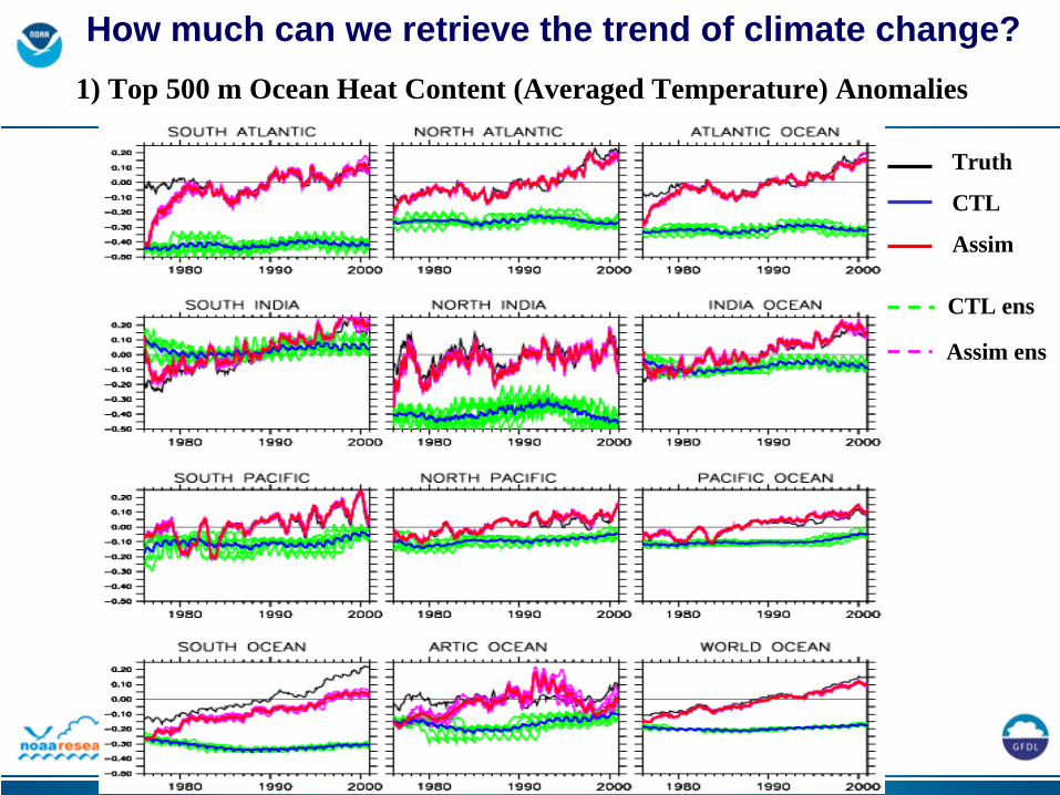
Truth

CTL

Assim

CTL ens

Assim ens

1) Top 500 m Ocean Heat Content (Averaged Temperature) Anomalies

How much can we retrieve the trend of climate change?

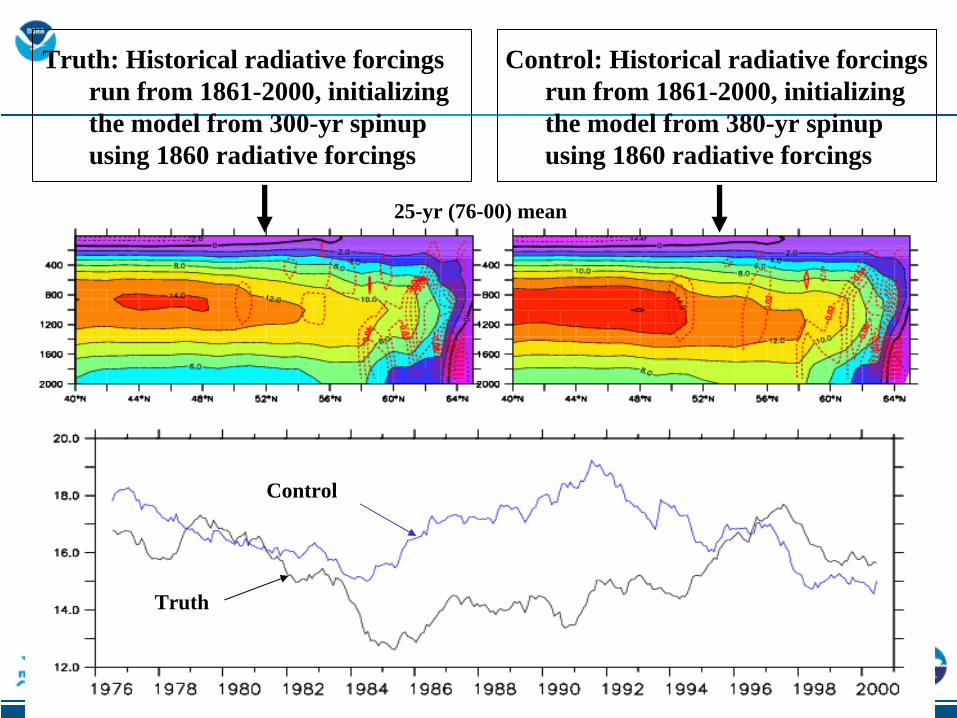
Truth: Historical radiative forcings run from 1861-2000, initializing the model from 300-yr spinupusing 1860 radiative forcings

Truth

Control

Control: Historical radiative forcings run from 1861-2000, initializing the model from 380-yr spinupusing 1860 radiative forcings

25-yr (76-00) mean

25-yr Time Mean of the Atlantic MOC

Truth


ODA (500m)T + Cov(T,S)

25-yr Time Mean of the Atlantic MOC

Truth


S. Zhang, personal communication

North Atlantic Max MOC from various ideal assimilation experiments

•

Based on 2005 Argo network and perfect model framework, the GFDL’s ensemble CDA system is able to reproduce the large time scale (decadal) trend of the Atlantic MOC by assimilating both ocean temperature and salinity.

•

These results are likely overly optimistic compared to real data assimilation

•

The variability of the Atlantic MOC is associated with large- scale THC’s heat/salt transport, sea surface forcing from atmosphere, fresh water forcing from ice and runoff and their interaction with the NA topography. Thus, atmospheric data constraint seems to improve the estimate of interannual timescale variability of the Atlantic MOC.

Remarks

Questions

Are we able to reproduce the hydrographyand transport in the Labrador basin in an idealized framework?

20th

century in-situ network is mainly

comprised of XBT and relatively sparse scientific transects. Is this network adequate?

What can we expect from the ARGO networknow that is is

almost fully deployed?

CM2.0 Variability

decadal variations in water mass volume(>= sigma2 = 36.8) in CM2. 5 year intervals.

85-80 90-85

95-90

EnKF estimation (idealized) using XBT network (500m) T+cov(t,s)

85-80 90-85

95-90 95- 90

truth

EnKF estimation using ARGO network T and S to 2000m

85-80 90-85

95-9095-

90 truth

Summary

• Idealized experiments indicate that proper initialization of N Atlantic requires temperature and salinity observations (using ocean in-situ constraint only)

• ARGO data to 2000m helps to recover changes in dense water volume in the Lab Sea

Gael Forget (MIT) has assessed the impact of ARGO profiles on ocean state estimates using the ECCO modeling infrastructure: MITgcm and its adjoint

Both

(i) ideal twin experiments and

(ii) ‘realistic’ calculations with real ARGO profiles and realistic model configurations

have been carried out.

Impact on the MOC of the Atlantic has been a particular focus

Assimilation of ARGO profiles dramatically improves the ability of the model to simulate the MOC and its heat transport.

Idealized experiments (simulated ARGO profiles / 1 year-long / Initial State control)

Error in MOC before assimilation Error after assimilation

Forget et al, a,b 2007, Ocean Modeling

Real ARGO profiles, May 2002-Apr 2003 (+climatology south of 30N & below 2000m)

before assimilation after assimilation

Atlantic MOC

20Sv13Sv

Forget et al, a,b 2007, Ocean Modeling

Real ARGO profiles, May 2002-Apr 2003 (+climatology south of 30N & below 2000m)

after assimilation

before assimilation

Courtesy J. Marshall

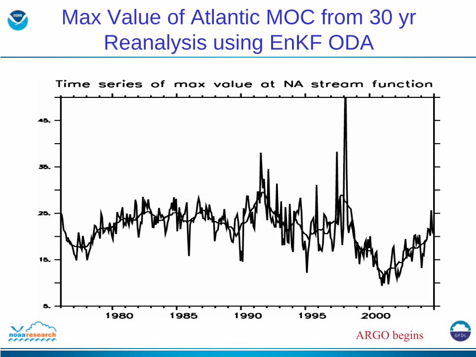
Max Value of Atlantic MOC from 30 yr Reanalysis using EnKF ODA

ARGO begins

Uncertainty in MOC projections

Increased realism from more realistic initial conditions?

Synthesis of two recent workshops on Atlantic climate

change, variability, and predictability

• Workshop 1: GFDL (Princeton), June 1-2, 2006

• Workshop 2: AOML (Miami), January 10-12, 2007

Overall purpose of pair of workshops was to develop a framework for coordinated activities to

(a) nowcast the state of the Atlantic (b) assess decadal predictability of the Atlantic and possible

atmospheric impacts(c) develop a prototype decadal prediction system, if warranted by (a)

and (b)

Workshop Goals

• Summarize aspects of what is known about decadal Atlantic variability, both in terms of observational analyses and physical mechanisms

• Discuss and assess what might potentially be predictable

• Discuss strategies for initializing models for decadal prediction

• Initiate efforts to catalyze US research on Atlantic predictability and predictions

GFDL/AOML Workshop 1 Presentations

• Impact of Atlantic variability on climate, including North American drought (Pacific dominant, but role for Atlantic)

• Predictability, both from statistical methods and dynamical models

• GFDL and CCSM models exhibit pronounced interdecadal variability in the Atlantic

• Initialization of models / nowcasting state of the Atlantic

GFDL/AOML Workshop 2 Presentations

• Summary of aspects of observational analyses of Atlantic decadal variability (surface and subsurface)

Phenomena of three time scales are of importance: decadal-scale fluctuationsmulti-decadal changes (AMO)trend

All need to be understood in order to describe Atlantic variability and change.

• Presentations on current observing systems in the Atlantic. This included a statement that with RAPID/MOC array in place, “… we estimate that the year-long average overturning can be defined with a standard error of 1 about Sv.”

• Presentation on paleo reconstructions for the Atlantic and their utility.

• Analysis of forced and internal variability components of Atlantic changes – suggestion that Atlantic multidecadal variability has a significant internal variability component

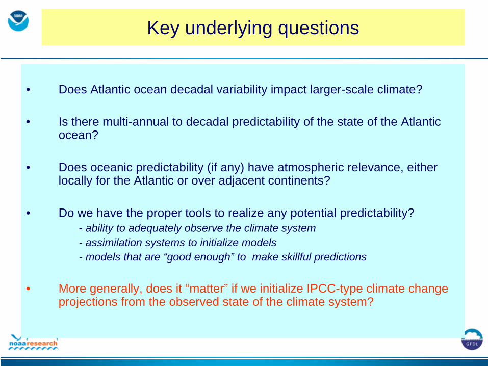
Key underlying questions

• Does Atlantic ocean decadal variability impact larger-scale climate?

• Is there multi-annual to decadal predictability of the state of the Atlantic ocean?

• Does oceanic predictability (if any) have atmospheric relevance, either locally for the Atlantic or over adjacent continents?

• Do we have the proper tools to realize any potential predictability?- ability to adequately observe the climate system- assimilation systems to initialize models- models that are “good enough” to make skillful predictions

• More generally, does it “matter” if we initialize IPCC-type climate change projections from the observed state of the climate system?

Workshop Recommendations

• Diagnostics Program – physical mechanisms of variability

• Predictability studies – which components have decadal predictability?

• Development of Improved Tools for Decadal Prediction and Analyses– Models– Observational/Assimilation systems

• Experimental Decadal Predictions (statistical, dynamical, multiple models)

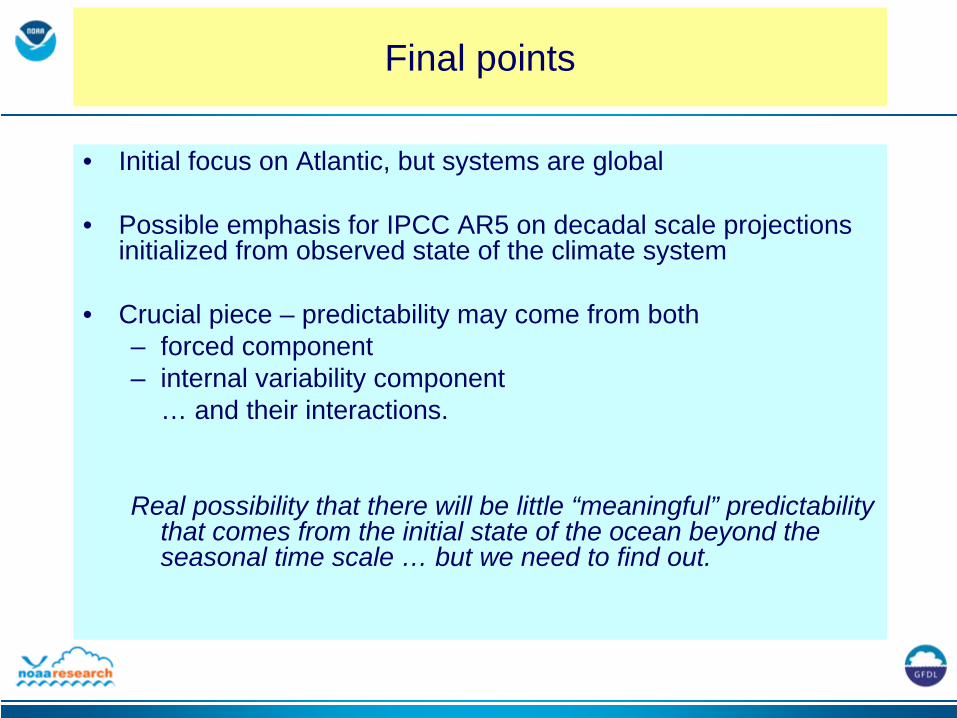
Final points

• Initial focus on Atlantic, but systems are global

• Possible emphasis for IPCC AR5 on decadal scale projections initialized from observed state of the climate system

• Crucial piece – predictability may come from both– forced component– internal variability component

… and their interactions.

Real possibility that there will be little “meaningful” predictability that comes from the initial state of the ocean beyond the seasonal time scale … but we need to find out.

atlantic decadal variability:combining observations and ... · pdf fileukgs ingv mri-eccosio...

Documents