asymptotic methods in optimization of multi-item inventory
TRANSCRIPT

393
___________________ Copyright © 2020 for this paper by its authors. Use permitted under Creative Commons License Attribution 4.0 International (CC BY 4.0).
Asymptotic methods in optimization of multi-item inventory management model
Lidiіa Horoshkova1,2[0000-0002-7142-4308], Ievgen Khlobystov3[0000-0002-9983-9062], Volodymyr Volkov1[0000-0002-1270-895X], Olha Holovan1[0000-0002-9410-3830],
Svitlana Markova1[0000-0003-0675-0235], Alexander Golub3[0000-0003-1823-2523] and Oleksandr Oliynyk1[0000-0003-0511-7681]
1 Zaporizhzhia National University, 66 Zhukovskogo Str., Zaporizhzhia, 69600, Ukraine [email protected], [email protected], [email protected],
[email protected] 2 Bila Tserkva Institute of Continuous Education of University of Educational Management,
52 Levanevskogo Str., Bila Tserkva, 09108, Ukraine [email protected]
3 National University of “Kyiv-Mohyla academy”, 2 Skovorody Str., Kyiv, 04070, Ukraine [email protected], [email protected]
Abstract. The study proposes asymptotic methods for optimizing multi-item inventory model. To achieve the objective of the study, formulas of the optimal value of multi-item delivery frequency based on the asymptotic approach under conditions of minor changes in the input parameters have been obtained. The discrete increase in the execution costs and inventory holding costs which depend on the “small parameter” as well as a gradual increase in periodic fluctuations in demand for products have been taken as variable parameters of the system. Easy-to-use analytical formulas for determining optimal order interval when ordering and inventory holding costs, as well as demand meet insufficient changes have been obtained. Testing of the proposed approach to the multi-item inventory model has been carried out on the example of HoReCa regional market segment. The proposed formulas allow to apply the obtained results for optimization and forecasting of decision-making in the system of procurement logistics of a company amid variation of input parameters describing changes of external and internal business environment.
Keywords: multi-item order, optimal order, delivery interval, small parameter, asymptotic methods.
1 Introducation
Sharpening of international and local competition leads to higher requirements for business processes’ competitiveness and efficiency. These could be achieved through the optimization of product, pricing, sales, innovation policy, as well as promotion policy. Therefore, forecasting and rational planning of all the subsystems of business
394
process management when minimizing operating and sales costs, strengthening cooperation and coordination between company’s structural units become relevant.
Solving these problems is not possible without the reduction of company’s inventory management costs. Excess stocks are frozen current assets, which do not bring additional benefits, but also require additional costs for their maintenance, holding, ensuring their appropriate quality.
The modern inventory management system is characterized by the introduction of the integrated approach to the inventory management within the internal logistics system, which is subject to the business strategy and provides the ability to determine the optimal inventory based on the demand forecast and changes in external and internal environment.
There are inventory management models and methods in the logistics system of an enterprise and corresponding software products that improve inventory management quality and efficiency in the market. Current decision-making support systems fulfill mainly the accounting functions, which significantly limits their effectiveness for companies’ management. To further improve these software products and ensure the possibility of their implementation to forecast various business activities, it is necessary to develop analytical tools for the inventory management system.
Asymptotic methods and approaches that allow to obtain analytical solutions of the applied problems, to assess sensitivity of these solutions to variations of system input parameters aimed at forecasting business activities are promising for the improvement of the analytical tools.
2 Literature review
Studies [1; 13] contain the main ideas of the asymptotic approach and perturbation techniques; they put their outlined features, advantages and limits of their application in various fields into layman's terms.
[7] is devoted to the technique of the asymptotic developments’ application in a series by small parameter degrees. This parameter is selected either artificially or emerges naturally in the model. The proposed technique assumes that the solution is sought in the form of the asymptotic sequence, which is taken as power function of a small parameter ε. Perturbation techniques are widely used in various natural science problems: solid mechanics and mathematics, in particular when solving differential equations. These methods are chosen as they allow to obtain an easy-to-use analytical formula to analyze system sensitivity to variable input parameters.
The scope of perturbation techniques can be extended to solving economic problems, modelling of relevant processes, managerial decision-making in general and one of the topical issues – inventory management issue in particular.
[10; 15] studies analyze features of the procurement logistics’ deterministic models building, which help managers in the decision-making process. The EOQ-model of the procurement logistics is made in [8] taking into account the shortage due to the possible defective products. The proposed model is limited by the minor discrete changes in execution costs. Implementation of the asymptotic methods to determine the order

395
quantity of a single-product inventory management problem amid insignificant discrete changes in execution costs is proposed in [6]. Analytical tools improvement using the asymptotic approach and taking into account the periodicity in the demand for products is implemented in [14]. However, the authors did not take into account the variability of storage costs. Further research referring to the application of asymptotic methods in the inventory management problems has been made in [2]. The authors proposed the model that considers execution and holding costs’ small gradual changes, as well as small periodic fluctuations in demand for products. However, the asymptotic approach was applied to the single-product inventory management problem.
In [22], a dynamic model of inventory management with the shift of the deficit of demand, which changes linearly, is built. The proposed model is aimed at determining the main efficiency indicators of the order management system with constant input parameters.
[12] studies the system of inventory planning for the industries producing nondurable goods. For small and medium-sized businesses in the food industry, the main issue is the compliance with the expiration dates of the proposed products. Therefore, the issue of reducing the amount of products, which past the expiry date, determining the optimal amount of products and time of multi-product order is especially relevant. Nevertheless, the authors use fixed parameters to determine the optimal order quantity and order period. Change in demand and inventory damage due to the sub-optimal inventory location or improper storage conditions are studied in [23]. Besides, the authors of the study consider the case when the inventory damage rate is distributed by the Weibull function, and inventory holding costs are discrete. Purchases of perishable goods are modelled in [3; 11] under the conditions of possible payment delays and inflation, but these models do not take into account possible fluctuations in demand for products. The study [24] concerned the integrated EOQ model building for the supplier`s and buyer`s monopoly who operate in the monopsony market diminishing ordering costs, but keeping inventory costs unchanged.
Researchers are trying to adapt the proposed models to the situations faced by companies who implement real production procedures in the logistics management system. For instance: fluctuations of demand, supply, component prices, inflation, consumer expectations, etc. [19] proposed the inventory management model in retail, which allows to maximize profit in the reverse logistics system, considering the level of supply and the term of delivery. Unlike most studies, [17] takes into account transport costs to obtain the optimal order, but the researchers propose the iterative approach, which is difficult to apply. Study [21] is another adaptation of the inventory management model considering spatial and temperature constraints on storage equipment. However, the results do not take into account changes in the execution and inventory costs.
The EOQ problem was studied in [26] for the case of the stochastic nature of input parameters and calculation of probability distribution using the geometric programming model. The stochastic problem of finding the optimal order quantity on a time interval is solved in [9]. However, the studies are mainly theoretical ones; there is lack of analytical formulas convenient for application and further analysis.

396
In [5] the multi-item problem of the inventory management amid insignificant changes of execution costs based on asymptotic approach was solved. Nonetheless, specification of the optimal order did not take into consideration the variability of inventory costs and demand.
The impact of the demand sensitive to marketing incentives on the solution of the multi-item EOQ-model problem for the two-level supply chain under the conditions of payment delay of outgoing inventory spending was considered in [4]. In [25] the multi-item inventory management model within limited warehouse space and application of the quantitative discount system was studied. The authors determined the optimal order applying Lagrange multiplier technique and the dynamic programming method, which is close to the Wagner-Within algorithm. These methods were compared to find the best solution to determine the number of orders. However, the authors use already known methods and algorithms to solve the applied problem.
In [20] genetic algorithm based on total inventory cost minimization was used to determine the quantity of raw materials’ multi-product batch. Nonetheless, inventory holding costs were based on the warehouse space during a period and unit`s space dimension.
The study [16] was devoted to the EOQ-model building, which is not without limitations. In particular, there are assumptions like deteriorating inventory quality, shortages, inventory space availability and the modesty of overall budget for purchasing of goods. [18] study proposed deficit-free multi-product EOQ model with inaccurate limitations for fragile goods. However, the proposed models do not take into account the variability of input parameters.
The analysis of well-known researchers’ works in the field of inventory management revealed that the proposed models allow to determine key inventory management system parameters, namely: order quantity, time interval between orders, etc. Still, there are difficulties in their application due to the complex mathematical apparatus and the impossibility of obtaining analytical formulas, convenient for the model behavior prediction with changing input parameters.
3 Research tasks
The study objective is optimization of inventory management multi-item model amid insignificant changes of input parameters using asymptotic methods. To achieve this objective, the following tasks were set:
1. To obtain the asymptotic formula of the multi-item inventory management model with a slight discrete spending spree on order execution and inventory holding;
2. To obtain the asymptotic formula of the multi-item inventory management model with variable order execution costs and small fluctuations in the amplitude of demand.

397
4 Results
4.1 Asymptotic expansion of the multi-item inventory management problem solution with a slight discrete spending spree on order execution and inventory holding
Inventory management model`s application allows company’s management to reduce fixed and variable production costs, order and sales costs. All costs related to the multi-item resources or goods ordering from one supplier are presented in the form of two components:
С0 – Costs formed when transporting, Сi – Costs depending on the activities when a specific order is being formed. Thus,
order execution costs k of product units у of one supplier are presented as (1).
퐶 = 퐶 + ∑ 퐶 = ∑ 퐶 (1)
In case of simultaneous delivery of k product groups, total costs are presented as (2) [10].
퐶∑ = ∑ 퐶 + ∑ 푆 퐶х → 푚푖푛, (2)
where Si – total consumption of і product during period, Схi – inventory costs for one unit produced, Т – delivery frequency, D – duration.
Under the conditions of model parameters with fixed values (2), the optimal value of multi-item delivery Topt frequency is determined as follows [10]:
푇 = 퐷 ∑∑
(3)
The assumption of model’s fixed parameters reduces possibility and effectiveness of its practical application. The asymptotic methods allow, without violating this condition, to perturb model’s parameters. Order execution costs are one of the following parameters fixed in the inventory management optimization model. In practice, this parameter may increase with certain repetitions caused by inflation, consumer and producer expectations, the “ratchet” effect, etc. To build the model it was assumed that during the specified time order execution costs, namely their transport component, rise repeatedly by l% and in n periods become 퐶 ⋅ 1 + %
%. By
introducing a small perturbation parameter, this correlation was presented as follows: 퐶 ⋅ (1 + 휀) , when ε<<1.
Practically, order execution costs and inventory holding costs rise due to the price boost for electricity and utilities. It was assumed in the study, that inventory holding costs surge every period by j%. Analogously, taking value 훽 = %
% (β<<1) as a small
parameter, it was obtained dependence of inventory as 퐶 (1 + 훽) . To improve the efficiency of the proposed model for manufacturing, it is advisable
to take into account different combinations of parameters n and m, ε and β. The
398
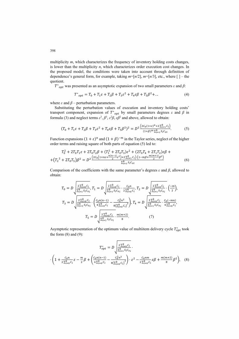
multiplicity m, which characterizes the frequency of inventory holding costs changes, is lower than the multiplicity n, which characterizes order execution cost changes. In the proposed model, the conditions were taken into account through definition of dependence’s general form, for example, taking m=[n/2], m=[n/3], etc., where [ ] – the quotient. 푇∗ was presented as an asymptotic expansion of two small parameters ε and β:
푇∗ = 푇 + 푇 휀 + 푇 훽 + 푇 휀 + 푇 휀훽 + 푇 훽 +. .. (4)
where ε and β – perturbation parameters. Substituting the perturbation values of execution and inventory holding costs’
transport component, expansion of 푇∗ by small parameters degrees ε and β in formula (3) and neglect terms ε3, β3, ε2β, εβ2 and above, allowed to obtain:
(푇 + 푇 휀 + 푇 훽 + 푇 휀 + 푇 휀훽 + 푇 훽 ) = 퐷( ) ∑
( ) ∑. (5)
Function expansions (1 + 휀) and (1 + 훽) in the Taylor series, neglect of the higher order terms and raising square of both parts of equation (5) led to:
푇 + 2푇 푇 휀 + 2푇 푇 훽 + (푇 + 2푇 푇 )휀 + (2푇 푇 + 2푇 푇 )휀훽 +
+ 푇 + 2푇 푇 훽 = 퐷( ) ∑ ⋅ ( )
∑ (6)
Comparison of the coefficients with the same parameter’s degrees ε and β, allowed to obtain:
푇 = 퐷 ∑∑
, 푇 = 퐷 ∑∑
⋅∑
, 푇 = 퐷 ∑∑
⋅ ,
푇 = 퐷 ∑∑
⋅ ( )∑
−∑
, 푇 = 퐷 ∑∑
⋅ ( )∑
,
푇 = 퐷 ∑∑
⋅ ( ). (7)
Asymptotic representation of the optimum value of multiitem delivery cycle 푇∗ took the form (8) and (9):
푇∗ = 퐷 ∑∑
⋅
⋅ 1 +∑
휀 − 훽 + ( )∑
−∑
⋅ 휀 −∑
휀훽 + ( )훽 , (8)
399
푇∗ = 푇 ⋅
⋅ 1 +∑
휀 − 훽 + ( )∑
−∑
⋅ 휀 −∑
휀훽 + ( )훽 . (9)
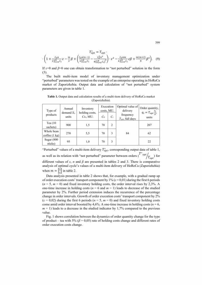
If ε=0 and β=0 one can obtain transformation to “not perturbed” solution in the form (3).
The built multi-item model of inventory management optimization under “perturbed” parameters was tested on the example of an enterprise operating in HoReCa market of Zaporizhzhia. Output data and calculation of “not perturbed” system parameters are given in table 1.
Table 1. Output data and calculation results of a multi-item delivery of HoReCa market (Zaporizhzhia).
Type of products
Annual demand Si,
units
Inventory holding costs,
Cxi, MU.
Execution costs, MU.
Optimal value of delivery
frequency Topt, full days
Order quantity, 푞 = 푇 ,
units С0 Сі
Tea (10 sachets)
900 1,5 70 2
84
207
Whole bean coffee (1 kg)
270 5,5 70 3 62
Sugar (800 sticks)
95 1,0 70 3 22
“Perturbed” values of a multi-item delivery 푇∗ , corresponding output data of table 1,
as well as its relation with “not perturbed” parameter between orders (푇∗
푇 ) for
different values of ε, n and β are presented in tables 2 and 3. There is comparative analysis of optimal cycle’s values of a multi-item delivery of HoReCa (Zaporizhzhia) when 푚 = in table 2.
Data analysis presented in table 2 shows that, for example, with a gradual ramp up of order execution costs’ transport component by 1% (ε = 0,01) during the first 6 periods (n = 5, m = 0) and fixed inventory holding costs, the order interval rises by 2,3%. A one-time increase in holding costs (n = 6 and m = 1) leads to decrease of the studied parameter by 2%. Further period extension induces the recurrence of the percentage change in order intervals. Growth of order execution costs’ transport component by 2% (ε = 0,02) during the first 6 periods (n = 5, m = 0) and fixed inventory holding costs come amid order interval boosted by 4,6%. A one-time increase in holding costs (n = 6, m = 1) leads to a decrease in the studied indicator by 1,7% compared to the previous value.
Fig. 1 shows correlation between the dynamics of order quantity change for the type of product – tea with 5% (β = 0,05) rate of holding costs change and different rates of order execution costs change.

400
Table 2. Comparative analysis of optimal cycle’s values of a multi-item delivery, β=0,05, 푚 = .
Period ε = 0,01 ε = 0,015 ε = 0,02
n m 푇∗
푇 푇∗ , full days 푇∗
푇 푇∗ , full days 푇∗
푇 푇∗ , full days
0 0 1,0000 84,00 1,0000 84,00 1,0000 84,00 1 0 1,0045 84,38 1,0067 84,56 1,0089 84,75 2 0 1,0090 84,75 1,0135 85,13 1,0180 85,51 3 0 1,0135 85,13 1,0203 85,70 1,0271 86,28 4 0 1,0181 85,52 1,0272 86,28 1,0363 87,05 5 0 1,0226 85,90 1,0341 86,86 1,0457 87,84 6 1 1,0018 84,15 1,0150 85,26 1,0283 86,38 7 1 1,0062 84,52 1,0217 85,82 1,0374 87,14 8 1 1,0107 84,89 1,0285 86,39 1,0466 87,91 9 1 1,0151 85,27 1,0353 86,96 1,0559 88,69 10 1 1,0196 85,64 1,0422 87,54 1,0652 89,48 11 1 1,0241 86,02 1,0491 88,12 1,0747 90,28 12 2 1,0025 84,21 1,0286 86,40 1,0555 88,66 13 2 1,0068 84,57 1,0353 86,96 1,0647 89,43 14 2 1,0111 84,94 1,0421 87,53 1,0740 90,22 15 2 1,0155 85,30 1,0489 88,11 1,0834 91,01 16 2 1,0199 85,67 1,0557 88,68 1,0930 91,81 17 2 1,0243 86,05 1,0627 89,26 1,1026 92,62 18 3 1,0019 84,16 1,0408 87,43 1,0814 90,84 19 3 1,0062 84,52 1,0475 87,99 1,0908 91,63 20 3 1,0105 84,88 1,0542 88,56 1,1002 92,42 21 3 1,0148 85,24 1,0610 89,13 1,1098 93,22 22 3 1,0191 85,60 1,0679 89,70 1,1195 94,04 23 3 1,0234 85,97 1,0748 90,29 1,1292 94,86 24 4 1,0002 84,02 1,0515 88,33 1,1062 92,92
Thus, with a gradual ramp up of order execution costs by 1,5% (ε=0,015) and 2% (ε=0,02) there is “perturbed” order quantity growth compared to the optimal (table 1) by 3,4% and 4,8% respectively (when n =5); by 4,8% and 7,7% (when n =11) and by 6,3% and 10,1% (when n =17). Periods which come amid holding costs shift (n = 6, m = 1), (n = 12, m = 2), etc. and gradual order execution costs surge by 2% (ε=0,02) face lower order quantity compared to the previous value by 1,9% respectively when n =6; by 1,8% when n = 12 and when n = 18.
Optimal periods of a multi-item delivery of HoReCa segment in Zaporizhzhia when β=0,05 and 푚 = are calculated in table 3.
Calculations given in table 3 reveal that at ε = 0.02 gradual execution costs change of a multi-item delivery leads to higher order interval by 0.9% at average at all intervals n, except for those periods when there is holding costs change. The change in inventory

401
holding costs at n = 12, m = 1 and n = 24, m = 2 leads to lower order interval by 1.8% and 2%, respectively, relative to the previous value.
Table 3. Calculation of optimal cycle`s values of a multi-item delivery of HoReCa (Zaporizhzhia), β=0,05, 푚 = .
Period ε = 0,01 ε = 0,015 ε = 0,02
n m 푇∗
푇 푇∗ , full days 푇∗
푇 푇∗ , full days 푇∗
푇 푇∗ , full days
0 0 1,0000 84,00 1,0000 84,00 1,0000 84,00 1 0 1,0045 84,38 1,0067 84,56 1,0089 84,75 2 0 1,0090 84,75 1,0135 85,13 1,0180 85,51 3 0 1,0135 85,13 1,0203 85,70 1,0271 86,28 4 0 1,0181 85,52 1,0272 86,28 1,0363 87,05 5 0 1,0226 85,90 1,0341 86,86 1,0457 87,84 6 0 1,0272 86,29 1,0411 87,45 1,0551 88,63 7 0 1,0319 86,68 1,0481 88,04 1,0646 89,43 8 0 1,0365 87,07 1,0552 88,64 1,0742 90,24 9 0 1,0412 87,46 1,0624 89,24 1,0840 91,05 10 0 1,0459 87,85 1,0696 89,85 1,0938 91,88 11 0 1,0506 88,25 1,0769 90,46 1,1037 92,71 12 1 1,0286 86,40 1,0561 88,71 1,0843 91,08 13 1 1,0332 86,78 1,0631 89,30 1,0940 91,89 14 1 1,0377 87,17 1,0702 89,90 1,1037 92,71 15 1 1,0423 87,56 1,0774 90,50 1,1136 93,54 16 1 1,0469 87,94 1,0846 91,10 1,1236 94,38 17 1 1,0516 88,33 1,0918 91,71 1,1336 95,23 18 1 1,0563 88,73 1,0991 92,33 1,1438 96,08 19 1 1,0610 89,12 1,1065 92,95 1,1541 96,94 20 1 1,0657 89,52 1,1139 93,57 1,1644 97,81 21 1 1,0704 89,92 1,1214 94,20 1,1749 98,69 22 1 1,0752 90,32 1,1290 94,83 1,1855 99,58 23 1 1,0800 90,72 1,1366 95,47 1,1961 100,48 24 2 1,0560 88,70 1,1127 93,47 1,1727 98,51 Comparing the results presented in table 2 and table 3, it can be concluded that the
increasing multiplicity of holding costs changes for products (m) in a multi-item delivery causes order interval contraction relative to the optimal. For example, higher holding costs (n = 24, m = 2) at ε = 0,02, β = 0,05 and when (n = 24, m = 4) come amid the contraction of the order interval from 98,51 to 92,92 full days or by 6%, which is quite significant.
Fig. 2 illustrates correlation between tea order quantity and parameters values ε and n.

402
Fig. 1. Correlation between tea order quantity and parameters values ε and n when β=0,05,
푚 = .
Fig. 2. Correlation between tea order quantity and parameters values ε and n at β=0,05,
푚 = .
The calculation revealed that n growth, which characterizes the frequency of order execution costs boost, to the value n = 11 at ε = 0.02 causes the increase in the order quantity to 10.4% relative to the optimal value. Shift of m (m = 1) leads to the decrease in order quantity by 1.8% compared to the previous value at ε = 0.02, and at (m = 2) leads to lower order quantity by 2.3%.
Figure 3 illustrates correlation of company’s total costs, operating in HoReCa segment in Zaporizhzhia from multiplicity of order and holding costs growth (n and 푚 = ).
One can see that higher order execution costs growth rate (fig. 3) causes total cost boost of a multi-item delivery. For example, parameter ε growth from 0,01 to 0,02 or by 1% leads to total costs boost by 3% at (n = 6, m = 1). Thenceforward, total costs growth takes place. Moreover, parameter’s ε impact becomes more significant. For example, at n = 12, m = 2 the difference between total costs values at ε = 0,01 and ε = 0,02 is 5,55%.
e=0,015
e=0,02
205210215220225230235240
0 2 4 6 8 10 12 14 16 18 20 22 24 26 28 30
q
n
208
218
228
238
248
258
0 2 4 6 8 10 12 14 16 18 20 22 24 26 28 30
e=0,01 e=0,015 e=0,02
q
n

403
Fig. 3. Correlation of customer’s total costs change to parameters values ε and β at 푚 = .
Fig. 4 illustrates shift of company’s total costs from execution costs in case 푚 = , i.e. inventory holding costs alter once in 12 periods.
Fig. 4. Correlation of company’s total costs’ change to parameters’ values ε and β at 푚 = .
676
726
776
826
876
926
976
1026
0 2 4 6 8 10 12 14 16 18 20 22 24 26 28 30
e=0,01, b=0,05 e=0,015, b=0,05 e=0,02, b=0,05
TC
n
404
Comparing the results demonstrated in fig. 3 and fig. 4, one can conclude that the contraction of multiplicity of holding costs changes m causes total costs reduction. For example, at ε = 0,01 and n = 6, m = 1 (fig. 3) total costs are UAH 711,64, and at ε = 0,01 and n = 6, m = 0 (fig. 4) they are UAH 694,49, which is 2,4% less. At ε = 0.02 and n = 6, m = 1 (fig. 3) total costs are UAH 730,95, and at ε = 0,02 and n = 6, m = 0 (fig. 4) they are UAH 713,33, which is 2,5% less. Thenceforward, this discrepancy is growing.
Thus, one can conclude that the higher periods’ multiplicity of ordering and holding costs of products (n and m) is, then period`s, order quantities of a multi-item delivery and execution costs’ cyclical fluctuations take place.
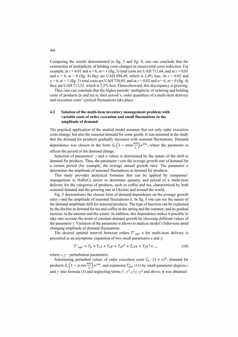
4.2 Solution of the multi-item inventory management problem with variable costs of order execution and small fluctuations in the amplitude of demand
The practical application of the studied model assumes that not only order execution costs change, but also the seasonal demand for some goods. It was assumed in the study that the demand for products gradually increases with seasonal fluctuations. Demand dependence was chosen in the form 푆 1 − 훼sin 푒 , where the parameter m affects the period of the demand change.
Selection of parameters’ γ and α values is determined by the nature of the shift in demand for products. Thus, the parameter γ sets the average growth rate of demand for a certain period (for example, the average annual growth rate). The parameter α determines the amplitude of seasonal fluctuations in demand for products.
This study provides analytical formulas that can be applied by companies’ management in HoReCa sector to determine quantity and period of a multi-item delivery for the categories of products, such as coffee and tea, characterized by both seasonal demand and the growing one in Ukraine and around the world.
Fig. 5 demonstrates the chosen form of demand dependence on the average growth rates γ and the amplitude of seasonal fluctuations α. In fig. 5 one can see the nature of the demand amplitude shift for seasonal products. The type of function can be explained by the decline in demand for tea and coffee in the spring and the summer, and its gradual increase in the autumn and the winter. In addition, this dependence makes it possible to take into account the trend of constant demand growth by choosing different values of the parameter γ. Variation of the parameter α allows to analyze model’s behaviour amid changing amplitude of demand fluctuations.
The desired optimal interval between orders 푇∗ a for multi-item delivery is presented as an asymptotic expansion of two small parameters ε and :
푇∗ = 푇 + 푇 휀 + 푇 훾 + 푇 휀 + 푇 휀훾 + 푇 훾 +. .., (10)
where ε, – perturbation parameters. Substituting perturbed values of order execution costs 퐶 ⋅ (1 + 휀) , demand for
products 푆 1 − 훼 푠푖푛 푒 , and expansion 푇∗ (11) by small parameter degrees ε and into formula (3) and neglecting terms ε3, 3, ε2, ε2 and above, it was obtained:

405
(푇 + 푇 휀 + 푇 훾 + 푇 휀 + 푇 휀훾 + 푇 훾 ) = 퐷( ) ∑
⋅ ∑. (11)
Fig. 5. Type of the demand dependence on the growth γ amplitude and seasonal fluctuations α
at 푚 = .
After expanding functions (1 + 휀) and 푒 in the Taylor series and neglecting high-order terms, after raising square of both parts of the equation (12), it was obtained:
푇 + 2푇 푇 휀 + 2푇 푇 훾 + (푇 + 2푇 푇 )휀 + (2푇 푇 + 2푇 푇 )휀훾 +
+ 푇 + 2푇 푇 훾 = 퐷( ) ∑ ⋅
∑. (12)
Comparison of the coefficients having the same parameters degrees ε і allowed to obtain:
푇 = 퐷 ∑
⋅∑, 푇 = 퐷 ∑
⋅∑⋅
∑,
푇 = 퐷 ∑
⋅∑⋅ ,
푇 = 퐷 ∑
⋅∑⋅ ( )
∑−
∑ (13)
푇 = 퐷 ∑
⋅∑⋅ ( )
∑, 푇 = 퐷 ∑
⋅∑⋅ .

406
“Perturbed” optimal cycle`s values of a multi-item delivery 푇∗ is (14)-(15):
푇∗ = 퐷 ∑
⋅∑⋅
⋅ 1 +∑
휀 − 훾 + ( )∑
−∑
⋅ 휀 −∑
휀훾 + 훾 , (14)
푇∗ = ⋅
⋅ 1 +∑
휀 − 훾 + ( )∑
−∑
⋅ 휀 −∑
휀훾 + 훾 (15)
To study interval sensitivity between orders of the multi-item inventory management model to changes in input parameters, namely to executive costs and fluctuations in demand, data of tables were used. Calculations were made for α = 0,05, γ = 0,01, with
values of the interval of a multi-item delivery 푇∗ and 푇∗
푇 for different values
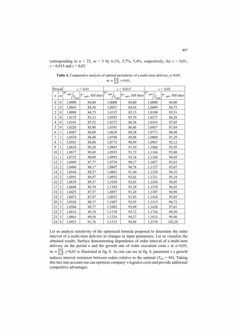
ε, n and α = 0,05 given in table 4. It provides comparative analysis of the optimal periodicity of a multi-item delivery for business in HoReCa sector (Zaporizhzhia) at 푚 = .
Data presented in table 4 reveal that fixed holding costs and demand, as well as order execution costs growth by 1,5% (ε = 0,015) during the first 12 periods (n = 11, m = 1) is characterized by the rising order interval from 84 up to 92 days or by 9,5%. When demand changes (n = 12, m = 2), the order period contracts by 2,2%, which can be explained by the type of function selected to approximate demand. Similar changes in the order interval are observed at ε = 0,02 and ε = 0,01: during the first 12 periods, the order interval goes up with its subsequent reduction. In the future, the trend of changing periods between orders is kept.
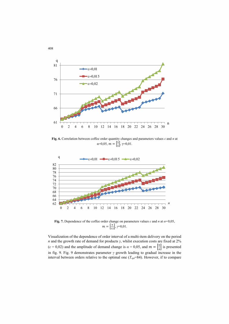
Correlation between coffee order quantity changes and parameters values ε and n at α = 0,05, 푚 = are presented in fig. 6. Fig. 6 shows that during the first 12 periods (n = 11, m = 1) when order execution costs change by 1% (ε = 0,01), 1,5% (ε = 0,015) and 2% (ε = 0,02), coffee orders increase by 8,1%, 9,7% and 12,9% compared to the initial period, respectively. Further change in demand (n = 12, m = 2) is characterized by the contraction of coffee orders by 2,9%, 1,5% and 1,4% compared to the previous value, respectively.
Dependence of the coffee order change on parameters values ε and n at α = 0,05, 푚 = is presented in fig. 7.
Comparing fig. 6 and fig. 7, one can conclude that extension of the period of change in demand for products (from 푚 = to 푚 = ) causes the decrease in optimal order’s number of amplitude fluctuations from 4 to 2. True value of coffee order quantity, corresponding to the “perturbed” interval, at n = 23, m = 1 exceeds values
407
corresponding to n = 23, m = 3 by 6,1%, 5,7%, 5,4%, respectively, for ε = 0,01, ε = 0,015 and ε = 0,02.
Table 4. Comparative analysis of optimal periodicity of a multi-item delivery, α=0,05, 푚 = , γ=0,01.
Period ε = 0,01 ε = 0,015 ε = 0,02
n m 푇∗
푇 푇∗ , full days 푇∗
푇 푇∗ , full days 푇∗
푇 푇∗ , full days
0 0 1,0000 84,00 1,0000 84,00 1,0000 84,00 1 0 1,0045 84,38 1,0067 84,56 1,0089 84,75 2 0 1,0090 84,75 1,0135 85,13 1,0180 85,51 3 0 1,0135 85,13 1,0203 85,70 1,0271 86,28 4 0 1,0181 85,52 1,0272 86,28 1,0363 87,05 5 0 1,0226 85,90 1,0341 86,86 1,0457 87,84 6 1 1,0487 88,09 1,0628 89,28 1,0771 90,48 7 1 1,0534 88,48 1,0700 89,88 1,0868 91,29 8 1 1,0581 88,88 1,0772 90,49 1,0967 92,12 9 1 1,0629 89,28 1,0845 91,10 1,1066 92,95 10 1 1,0677 89,69 1,0919 91,72 1,1166 93,80 11 1 1,0725 90,09 1,0993 92,34 1,1268 94,65 12 2 1,0449 87,77 1,0734 90,17 1,1027 92,63 13 2 1,0496 88,17 1,0807 90,78 1,1127 93,47 14 2 1,0544 88,57 1,0881 91,40 1,1229 94,32 15 2 1,0591 88,97 1,0955 92,02 1,1331 95,18 16 2 1,0639 89,37 1,1030 92,65 1,1434 96,05 17 2 1,0688 89,78 1,1105 93,28 1,1539 96,92 18 3 1,0425 87,57 1,0857 91,20 1,1307 94,98 19 3 1,0473 87,97 1,0932 91,83 1,1410 95,85 20 3 1,0520 88,37 1,1007 92,45 1,1515 96,72 21 3 1,0568 88,77 1,1082 93,09 1,1620 97,61 22 3 1,0616 89,18 1,1158 93,72 1,1726 98,50 23 3 1,0665 89,58 1,1234 94,37 1,1833 99,40 24 4 1,0923 91,76 1,1533 96,88 1,2176 102,28
Let us analyze sensitivity of the optimized formula proposed to determine the order interval of a multi-item delivery to changes in input parameters. Let us visualize the obtained results. Surface demonstrating dependence of order interval of a multi-item delivery on the period n and the growth rate of order execution costs ε at α=0,05, 푚 = , γ=0,01 is illustrated in fig. 8. As one can see in fig. 8, parameter`s ε growth induces interval extension between orders relative to the optimal (Topt = 84). Taking this fact into account one can optimize company’s logistics costs and provide additional competitive advantages.
408
Fig. 6. Correlation between coffee order quantity changes and parameters values ε and n at
α=0,05, 푚 = , γ=0,01.
Fig. 7. Dependence of the coffee order change on parameters values ε and n at α=0,05,
푚 = , γ=0,01.
Visualization of the dependence of order interval of a multi-item delivery on the period n and the growth rate of demand for products γ, whilst execution costs are fixed at 2% (ε = 0,02) and the amplitude of demand change is α = 0,05, and 푚 = is presented in fig. 9. Fig. 9 demonstrates parameter γ growth leading to gradual increase in the interval between orders relative to the optimal one (Topt=84). However, if to compare
61
66
71
76
81
0 2 4 6 8 10 12 14 16 18 20 22 24 26 28 30
e=0,01
e=0,015
e=0,02
q
n
6264666870727476788082
0 2 4 6 8 10 12 14 16 18 20 22 24 26 28 30
q
n
e=0,01 e=0,015 e=0,02

409
the order intervals for different values of the parameter γ, one can see the tendency to the decreased interval between orders with growing value of γ.
Fig. 8. Dependence of order interval of a multi-item delivery on the period n and the growth
rate of order execution costs ε at α=0,05, 푚 = , γ=0,01.
Fig. 9. Dependence of order interval of a multi-item delivery on the period n and the growth
rate of demand for products γ at α=0,05, 푚 = , ε =0,02.
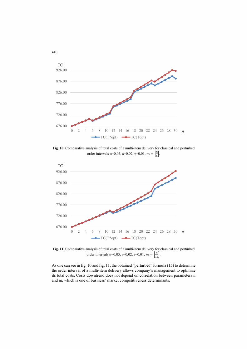
Let us analyze total costs of a multi-item delivery taking into consideration execution costs changes and gradual growth of demand for classical and perturbed order intervals (α=0,05, ε=0,02, γ=0,01). Their comparison for 푚 = and 푚 = respectively is presented in fig. 10 and fig. 11.
00.007
0.014
80
90
100
110
0 2 4 6 8 10 12 14 16 18 20 22 24 26 28 30e
T*
n
110-111 100-110 90-100 80-90
410
Fig. 10. Comparative analysis of total costs of a multi-item delivery for classical and perturbed
order intervals α=0,05, ε=0,02, γ=0,01, 푚 = .
Fig. 11. Comparative analysis of total costs of a multi-item delivery for classical and perturbed
order intervals α=0,05, ε=0,02, γ=0,01, 푚 = .
As one can see in fig. 10 and fig. 11, the obtained “perturbed” formula (15) to determine the order interval of a multi-item delivery allows company’s management to optimize its total costs. Costs downtrend does not depend on correlation between parameters n and m, which is one of business’ market competitiveness determinants.
676.00
726.00
776.00
826.00
876.00
926.00
0 2 4 6 8 10 12 14 16 18 20 22 24 26 28 30
TC(T*opt) TC(Topt)
ТС
п
676.00
726.00
776.00
826.00
876.00
926.00
0 2 4 6 8 10 12 14 16 18 20 22 24 26 28 30
TC(T*opt) TC(Topt)
ТС
п

411
5 Discussion of the results of multi-item inventory model’s optimization based on the asymptotic methods
The asymptotic approach proposed for solving the multi-item inventory management model, in contrast to the classical approach, allows to vary system input parameters, which significantly expands the scope of this model`s application. In the study, the degree of system parameters variation is insignificant as percentage of the initial values. Input parameters such as order execution and inventory holding costs (by introduction of small values rate of change by periods) and demand for products (by introduction of amplitude shift and growth rate parameters by periods) were varied.
Execution costs growth rate is characterized by a small parameter ε. Interval from 0 to 0,02 (i.e. 0–2,0%) was considered as the parameter’s range of changes. Inventory holding costs growth rate is determined by the parameter β, which range of variation was limited by the interval from 0 to 0,05 (i.e. 0-5,0%). These parameters values can be explained by their specificity. For instance, parameter β had bigger range of change than ε, because the percentage utility costs growth is less frequent, but is more substantial.
The gradual growth rate of demand for products is characterized by the parameter γ. The interval from 0 to 0,02 (i.e. 0–2,0%) was taken as the range of change of this parameter in the study. Parameter α was chosen as the parameter characterizing the amplitude of seasonal demand fluctuations, which range was set at 0,05 (i.e. 5%). However, to illustrate the change in the nature of the demand function, this parameter was also set at 3%. The choice of parameters α and γ is determined by the specifics of HoReCa market segment and the supplied products (coffee, tea, sugar).
The asymptotic formulas obtained for the multi-item supply model also contain the parameters n and m. These parameters specify periods of execution costs change (n) and holding costs change (m). In addition, parameter m typifies periods of seasonal demand change and growth. So, as utility costs change occurs not so often as the change in order execution costs (namely, its transport component), the parameter m was chosen as a mathematical function of quotient m = [n / 6] and m = [n / 12], which corresponds to the parameter change once every six months or once a year, respectively.
Solution of the multi-item supply problem amid small discrete execution and inventory holding costs growth was obtained in the form of a two-parameter asymptotic formula (9). Assessment of the developed model’s sensitivity to changes in the input parameters revealed that the relative deviation of the time interval between orders (tables 2, 3) varies from 0% to +19% depending on the period. Calculation of order quantity for different values of the parameter ε (fig. 2) shows the growing tendency of order quantity with this parameter’s boost.
The asymptotic formula for determining the optimal order period of a multi-item supply under the condition of changing order costs and periodic demand growth for products was obtained in the form (15). The study of the obtained “perturbed” formula’s sensitivity to changes in input parameters (table 4) found out that the time interval between orders depends on the periods of input parameters change, as well as of their percentage change. Calculation of the time interval deviation between orders according to the formula (15) (table 4) at different values of the input parameters shows an upward

412
trend. Thus, the deviation can range from 0% to +22% for the respective periods. Calculation of the interval between orders for different values of the parameter ε demonstrates its growth with respect to the optimal. Considering this fact, one can optimize company’s logistics costs and provide additional advantages to the competitiveness.
Among the limitations of the study one should note application of the selected forms to approximate functions that characterize order execution and holding costs change, as well as seasonal demand function for products.
The resulting asymptotic solutions of the multi-item inventory management model are of practical significance, as the resulting “perturbed” formulas are convenient for companies’ management to forecast possible changes in company’s logistics system amid demand, order and holding costs variation.
The proposed asymptotic method for two parameters is the development of analytical tools for the procurement and inventory management in contrast to [7; 10]. In particular, the proposed formulas allow to apply the obtained results for optimization and forecasting of decision-making in the system of procurement logistics of a company amid variation of input parameters describing changes of external and internal business environment. An easy-to-use model that takes into account demand and costs shift makes it possible to optimize the process of business procurement organization, to forecast company’s total costs in order to ensure its market competitive position.
Prospects for further research are associated with building of asymptotic solutions of inventory management models with minor changes in input parameters under scarce resources, including warehouse space, vehicle capacity, available current assets, etc.
6 Conclusions
Optimization streams of the multi-item inventory management model under the condition of insignificant changes of input parameters based on asymptotic methods were proposed.
1. Asymptotic formula to determine the order period of the multi-item inventory management model with a slight discrete order execution and inventory holding costs growth was obtained. Formula contains two small parameters that characterize order execution and inventory holding costs growth rate in accordance with the period. It makes it possible to specify the order execution period and the order quantity of product categories included into a multi-item delivery. Thus, the higher periods’ multiplicity of ordering and holding costs of products (n and m) is, then period’s cyclical fluctuations and the order quantity with the growing tendency take place. The improved asymptotic formula is convenient for business processes’ planning and forecasting.
2. Asymptotic formula of the multi-item inventory management model with variable order execution costs and insignificant fluctuations in the amplitude of growing demand was made. Order execution costs growth rate and the demand growth rate, which depend on the period and the functions selected for approximation, were chosen as small parameters. The study of the “perturbed” interval`s deviation nature
413
between orders under the different conditions of gradual order execution costs and demand growth found out that it basically goes up even with minor changes in the model’s input parameters. The parameter growth, which characterizes the demand growth rate, causes gradual interval value boost between orders relative to the optimal, used for forecasting and logistics decision-making by the company’s management.
References
1. Andrianov, I.V., Manevitch, L.I.: Asymptology: Ideas, Methods, and Applications. Springer US, New York (2002). doi:10.1007/978-1-4419-9162-1
2. Bikulov, D., Holovan, O., Oliynyk, O., Shupchynska K., Markova, S., Chkan, A., Makazan, E., Sukhareva, K., Kryvenko, O.: Optimization of inventory management models with variable input parameters by perturbation methods. Eastern-European Journal of Enterprise Technologies 3(105), 6–15 (2020). doi:10.15587/1729-4061.2020.204231
3. Brodetskii, G.L.: Influence of order payment delays on the efficiency of multiitem reserve control models. Automation and Remote Control 11, 94–104 (2017). doi:10.1134/S0005117917110078
4. Cárdenas-Barrón, L.E., Sana, S.S.: Multi-item EOQ inventory model in a two-layer supply chain while demand varies with promotional effort. Applied Mathematical Modelling 39(21), 6725-6737 (2015). doi:10.1016/j.apm.2015.02.004
5. Golovan, O.O., Oliynyk O., Kovalenko, N.V.: Adaptation of logistics management systems using asymptotic methods. Actual problems of economics 5, 395–401 (2016)
6. Golovan, O.O., Oliynyk O., Shyshkin, V.O.: Logistic business processes modelling using asymptotic methods. Actual problems of economics 9, 428–433 (2015)
7. Gristchak, V.Z.: A Hybrid Asymptotic Methods and Technique of Application. Zaporizhzhya National University, Zaporozhye, (2009)
8. Jaggi, C.K., Goel, S.K., Mittal, M.: Credit Financing in Economic Ordering Policies for Defective Items with Allowable Shortages. Applied Mathematics and Computation 219(10), 5268–5282 (2013). doi:10.1016/j.amc.2012.11.027
9. Kuzmin, O. V., Tungalag, N., E`nkhbat, R., E`rde`ne`bat, M.: Optimization approach to the stochastic problem of the stocks control. Modern technologies. System analysis. Modeling3(55), 106–110 (2017). doi: 10.26731/1813-9108.2017.3(55).106-110
10. Lukinskiy, V.S, Lukinskiy, V.V., Pletneva, N. G.: Logistics and supply chain management. Yurayt, Moscow (2016)
11. Mittal, M., Khanna, A., Jaggi, C.K.: Retailer's ordering policy for deteriorating imperfect quality items when demand and price are time-dependent under inflationary conditions and permissible delay in payments. International Journal of Procurement Management 10(4), 461–494 (2017). doi:10.1504/IJPM.2017.085037
12. Nasution, A.A., Rizkya, I., Ksyahpturib, Mariana, R.R.: Iventory policy for multi item products by short expiration period. In: 2nd Talenta Conference on Engineering, Science and Technology, TALENTA-CEST 2019; Grand Aston Hotel Medan; Indonesia; 17 October 2019 Volume 801, Issue 1, 2 June 2020 (2020). doi:10.1088/1757-899X/801/1/012110
13. Nayfeh, A.H.: Introduction to Perturbation Techniques. Wiley, New York (2011) 14. Oliynyk, O., Golovan, O.O., Мakazan, E.V.: Directions of analytical tools improvement in
management of machine-building enterprise’s logistic subsystem. Actual problems of economics 9, 383–390 (2016)

414
15. Pentico, D.W., Drake, M.J.: A Survey of Deterministic Models for the EOQ and EPQ with Partial Backordering. European Journal of Operational Research 214(2), 179–198 (2011). doi:10.1016/j.ejor.2011.01.048
16. Rabbania, M., Rezaeia, H., Lashgarib, M., Farrokhi-Aslb. H.: Vendor managed inventory control system for deteriorating items using metaheuristic algorithms. Decision Science Letters 7(1), 25–38 (2018). doi:10.5267/j.dsl.2017.4.006
17. Rasay, H., Golmohammadi, A.M.: Modeling and Analyzing Incremental Quantity Discounts in Transportation Costs for a Joint Economic Lot Sizing Problem. Iranian Journal of Management Studies 13(1), 23–49 (2020). doi: 10.22059/IJMS.2019.253476.673494
18. Saha, A., Roy, A., Kar, S., Maiti, M.: Inventory models for breakable items with stock dependent demand and imprecise constraints. Mathematical and Computer Modelling 52(9–10), 1771–1782 (2010). doi:10.1016/j.mcm.2010.07.004
19. Sanni, S., Jovanoski, Z., Sidhu, H.S.: An economic order quantity model with reverse logistics program. Operations Research Perspectives 7, 100133 (2020). doi:10.1016/j.orp.2019.100133
20. Saraswati, D., Sari, D.K., Johan, V.: Using genetic algorithm to determine the optimal order quantities for multi-item multi-period under warehouse capacity constraints in kitchenware manufacturing. IOP Conference Series: Materials Science and Engineering 273, 012020 (2017). doi:10.1088/1757-899X/245/1/012020
21. Satiti, D., Rusdiansyah, A., Dewi, R.S.: Modified EOQ Model for Refrigerated Display’s Shelf-Space Allocation Problem. IOP Conference Series: Materials Science and Engineering 722, 012014 (2020). doi:10.1088/1757-899X/722/1/012014
22. Tripathi, R.P., Singh, D., Mishra, T.: Economic Order Quantity with Linearly Time Dependent Demand Rate and Shortages. Journal of Mathematics and Statistics 11(1), 21–28 (2015). doi:10.3844/jmssp.2015.21.28
23. Tyagi, A.P.: An Optimization of an Inventory Model of Decaying-Lot Depleted by Declining Market Demand and Extended with Discretely Variable Holding Costs. International Journal of Industrial Engineering Computations 5(1), 71–86 (2014). doi:10.5267/j.ijiec.2013.09.005
24. Vijayashree, M., Uthayakumar, R.: A single-vendor and a single-buyer integrated inventory model with ordering cost reduction dependent on lead time. Journal of Industrial Engineering International volume 13, 393–416 (2017). doi:10.1007/s40092-017-0193-y
25. Yassa, R.I., Ikatrinasari, Z.F.: Determination of multi-item inventory model with limitations of warehouse capacity and unit discount in leading garment industry in Indonesia. International Journal of Mechanical and Production Engineering Research and Development 9(2), 161–170 (2019)
26. Yousefli, A., Ghazanfari, M.: A Stochastic Decision Support System for Economic Order Quantity Problem. Advances in Fuzzy Systems 2012, 650419 (2012). doi:10.1155/2012/650419