asymptotic analysis of objectives based on fisher
TRANSCRIPT

Journal of Machine Learning Research 18 (2017) 1-41 Submitted 3/15; Revised 2/17; Published 4/17
Asymptotic Analysis of Objectives Based on FisherInformation in Active Learning
Jamshid Sourati [email protected] of Electrical and Computer EngineeringNortheastern UniversityBoston, MA 02115 USA
Murat Akcakaya [email protected] of Electrical and Computer EngineeringUniversity of PittsburghPittsburgh, PA 15261 USA
Todd K. Leen [email protected] UniversityWashington D.C. 20057 USA
Deniz Erdogmus [email protected]
Jennifer G. Dy [email protected]
Department of Electrical and Computer Engineering
Northeastern University
Boston, MA 02115 USA
Editor: Qiang Liu
Abstract
Obtaining labels can be costly and time-consuming. Active learning allows a learningalgorithm to intelligently query samples to be labeled for a more efficient learning. Fisherinformation ratio (FIR) has been used as an objective for selecting queries. However, littleis known about the theory behind the use of FIR for active learning. There is a gap betweenthe underlying theory and the motivation of its usage in practice. In this paper, we attemptto fill this gap and provide a rigorous framework for analyzing existing FIR-based activelearning methods. In particular, we show that FIR can be asymptotically viewed as anupper bound of the expected variance of the log-likelihood ratio. Additionally, our analysissuggests a unifying framework that not only enables us to make theoretical comparisonsamong the existing querying methods based on FIR, but also allows us to give insight intothe development of new active learning approaches based on this objective.
Keywords: classification active learning, Fisher information ratio, asymptotic log-loss,upper-bound minimization.
1. Introduction
In supervised learning, a learner is a model-algorithm pair that is optimized to (semi) auto-matically perform tasks, such as classification, or regression using information provided by
c©2017 Jamshid Sourati, Murat Akcakaya, Todd K. Leen, Deniz Erdogmus and Jennifer G. Dy.
License: CC-BY 4.0, see https://creativecommons.org/licenses/by/4.0/. Attribution requirements are providedat http://jmlr.org/papers/v18/15-104.html.

Sourati, Akcakaya, Leen, Erdogmus and Dy
an external source (oracle). In passive learning, the learner has no control over the informa-tion given. In active learning, the learner is permitted to query certain types of informationfrom the oracle (Cohn et al., 1994). Usually there is a cost associated with obtaining infor-mation from an oracle; therefore an active learner will need to maximize the informationgained from queries within a fixed budget or minimize the cost of gaining a desired level ofinformation. A majority of the existing algorithms restrict to the former problem, to getthe most efficiently trained learner by querying a fixed amount of knowledge (Settles, 2012;Fu et al., 2013).
Active learning is the process of coupled querying/learning strategies. In such an algo-rithm, one needs to specify a query quality measure in terms of the learning method thatuses the new information gained at each step of querying. For instance, information theo-retic measures are commonly employed in classification problems to choose training sampleswhose class labels, considered as random variables, are most informative with respect to thelabels of the remaining unlabeled samples. This family of measures is particularly helpfulwhen probabilistic approaches are used for classification. Among these objectives, Fisherinformation criterion is very popular due to its relative ease of computation compared toother information theoretic objectives, desirable statistical properties and existence of ef-fective optimization techniques. However, as we discuss in this manuscript, this objectiveis not well-studied in the classification context and there seems to be a gap between theunderlying theory and the motivation of its usage in practice. This paper is an attemptto fill this gap and also provide a rigorous framework for analyzing the existing queryingmethods based on Fisher information.
From the statistical point of view, we characterize the process of constructing a classifierin three steps as follows: (1) choosing the loss and risk functions, (2) building a decision rulethat minimizes the risk, and (3) modeling the discriminant functions of the decision rule.For instance, choosing the simple 0/1 loss and its a posteriori expectation as the risk, incursthe Bayes rule as the optimal decision (Duda et al., 1999), where the discriminant functionis the posterior distribution of the class labels given the covariates. For this type of risk,discriminative models that directly parametrize the posteriors, such as logistic regression,are popularly used to learn the discriminant functions (Bishop, 2006). In order to bettercategorize the existing techniques, we break an active learning algorithm into the followingsub-problems:
(i) (Query Selection) Sampling a set of covariates x1, ...,xn from the training marginal1,whose labels y1, ..., yn are to be requested from an external source of knowledge (theoracle). The queried covariates together with their labels form the training data set.
(ii) (Inference) Estimating parameters of the posterior model based on the training dataset formed in the previous step.
(iii) (Prediction) Making decisions regarding class labels of the test covariates sampledfrom the test marginal.
These three steps can be carried out iteratively. Note that the query selection sub-problem is formulated in terms of the distribution from which the queries will be drawn.
1. Throughout this paper, marginal distribution or simply distribution refers to the distribution of covari-ates, while joint distribution is used for pairs of the covariates and their class labels.
2

Asymptotic Analysis of Objectives Based on Fisher Information in Active Learning
Ideally, queries (or the query distribution) are chosen such that they increase the expectedquality of the classification performance measured by a particular objective function. Thisobjective can be constructed from two different perspectives: based on the accuracy of theparameter inference or the accuracy of label prediction. In the rest of the manuscript,accordingly, we refer to the algorithms that use these two types of objectives as inference-based or prediction-based algorithms, respectively.
Most of the inference-based querying algorithms in classification aim to choose queriesthat maximize the expected change in the objective of the inference step (Settles et al.,2008; Guo and Schuurmans, 2008) or Fisher information criterion (Hoi et al., 2006; Settlesand Craven, 2008; Hoi et al., 2009; Chaudhuri et al., 2015b). On the other hand, the widerange of studies in prediction-based active learning includes a more varied set of objectives:for instance, the prediction error probability2 (Cohn et al., 1994; Freund et al., 1997; Zhuet al., 2003; Nguyen and Smeulders, 2004; Dasgupta, 2005; Dasgupta et al., 2005; Balcanet al., 2006; Dasgupta et al., 2007; Beygelzimer et al., 2010; Hanneke et al., 2011; Hanneke,2012; Awasthi et al., 2013; Zhang and Chaudhuri, 2014), variance of the predictions (Cohnet al., 1996; Schein and Ungar, 2007; Ji and Han, 2012), uncertainty of the learner withrespect to the unknown labels as evaluated by the entropy function (Holub et al., 2008),mutual information (Guo and Greiner, 2007; Krause et al., 2008; Guo, 2010; Sourati et al.,2016), and margin of the samples with respect to the trained hyperplanar discriminantfunction (Schohn and Cohn, 2000; Tong and Koller, 2002).
In this paper, we focus on the Fisher information criterion used in classification ac-tive learning algorithms. These algorithms use a scalar function of the Fisher informationmatrices computed for parametric models of training and test marginals. In the classifi-cation context, this scalar is sometimes called Fisher information ratio (FIR) (Settles andCraven, 2008) and its usage is motivated by older attempts in optimal experiment designfor statistical regression methods (Fedorov, 1972; MacKay, 1992; Cohn, 1996; Fukumizu,2000).
Among the existing FIR-based classification querying methods, only the very first oneproposed by Zhang and Oles (2000) approached the FIR objective from a parameter infer-ence point of view. Using a maximum likelihood estimator (MLE), they claimed (with theproof skipped) that FIR is asymptotically equal to the expectation of the log-likelihood ratiowith respect to both test and training samples (see sub-problem i above). Later on, Hoi et al.(2006) and Hoi et al. (2009), inspired by Zhang and Oles (2000), used FIR in connectionwith a logistic regression classifier with the motivation of decreasing the labels’ uncertaintyand hence the prediction error. Settles and Craven (2008) employed this objective with thesame motivation, but using a different approximation and optimization technique. More re-cently, Chaudhuri et al. (2015b) showed that even finite-sample FIR is closely related to theexpected log-likelihood ratio of an MLE-based classifier. However, their results are derivedunder a different and rather restricting set of conditions and assumptions: they focused onthe finite-sample case where the test marginal is a uniform PMF and the proposal marginalis a general PMF (to be determined) over a finite pool of unlabeled samples. Moreover,they assumed that the conditional Fisher information matrix is assumed to be independentof the class labels. Here, in a framework similar to Zhang and Oles (2000) but with a more
2. Prediction error probability is indeed the frequentist risk function of 0/1 loss, and is also known asgeneralization error.
3

Sourati, Akcakaya, Leen, Erdogmus and Dy
expanded and different derivation, we discuss a novel theoretical result based on whichFIR is related to an MLE-based inference step for a large number of training data. Morespecifically, under certain regularity conditions required for consistency of MLE and in theabsence of model mis-specification, and with no restricting assumptions on the form of testor training marginals, we show that FIR can be viewed as an upper bound for the expectedvariance of the asymptotic distribution of the log-likelihood ratio. Inspired by Chaudhuriet al. (2015b), we also show that under certain extra conditions, this relationship holds evenin finite-sample case.
There are two practical issues in employing FIR as a query selection objective: its com-putation and optimization. First, computing the Fisher information matrices is usuallyintractable, except for very simple distributions; also FIR depends on the true marginal,which is usually unknown. Therefore, even if the computations are tractable, approxima-tions have to be used for evaluating FIR. Second, the optimization of FIR is straightforwardonly if a single query is to be selected per iteration, or when the optimization has continuousdomain (e.g., optimizing to get the real parameters of the query marginal as in Fukumizu,2000). However, the optimization becomes NP-hard when multiple queries are to be selectedfrom a countable set of unlabeled samples (pool-based batch active learning). Heuristics havebeen used to approximate such combinatorial optimization, such as greedy methods (Settlesand Craven, 2008) and relaxation to continuous domains (Guo, 2010). Another strategy isto take advantage of monotonic submodularity of the objective set functions. If the objec-tive is shown to be monotonically submodular, efficient greedy algorithms can be used foroptimization with guaranteed tight bounds (Krause et al., 2008; Azimi et al., 2012; Chenand Krause, 2013). Regarding FIR, Hoi et al. (2006) proved that, when a logistic regressionmodel is used, a Monte-Carlo simulation of this objective is a monotone and submodularset function in terms of the queries.
In addition to our theoretical contribution in asymptotically relating FIR to the log-likelihood ratio, we clarify the differences between some of the existing FIR-based queryingmethods according to the techniques that they use to address the evaluation and optimiza-tion issues. Furthermore, we show that monotonicity and submodularity of Monte-Carloapproximation of FIR can be extended from logistic regression models to any discriminativeclassifier. Here is a summary of our contributions in this paper:
• Establishing a relationship between the Fisher information matrix of the query dis-tribution and the asymptotic distribution of the log-likelihood ratio (Section 4.1);
• Showing that FIR can be viewed as an upper bound of the expected asymptoticvariance of the log-likelihood ratio, implying that minimizing FIR, as an active learn-ing objective, is asymptotically equivalent to upper-bound minimization of the ex-pected variance of the log-likelihood ratio, as a measure of inference performance(Section 4.2);
• Proving that under certain assumptions, the above-mentioned asymptotic relationshipalso holds for finite-sample estimation of FIR (Section 5.1.1);
• Discussing different existing methods for coping with practical issues in using FIR inquerying algorithms (Section 5.1), and accordingly providing a unifying frameworkfor existing FIR-based active learning methods (Section 5.2).
4

Asymptotic Analysis of Objectives Based on Fisher Information in Active Learning
• Proving submodularity for the Monte-Carlo simulation of FIR under any discrimi-native classifier, assuming a pool-based active learning which enables access to ap-proximations of Fisher information matrices of both test and training distributions(Lemma 7 and Theorem 8).
Before going through the main discussion in Section 4, we formalize our classificationmodel assumptions, set the notations and review the basics and some of the key properties ofour inference method, maximum likelihood estimation, in Sections 2 and 3. The statisticalbackground required to follow the remaining sections is given in Appendix A.
2. The Framework and Assumptions
In this paper, we deal with classification problems, where each covariate, represented by afeature vector x in vector space X, is associated with a numerical class label y. Assumingthat there are 1 < c <∞ classes, y can take any integer among the set 1, ..., c. Supposethat the pairs (x, y) are distributed according to a parametric joint distribution p(x, y|θ),with the parameter space denoted by Ω ⊆ Rd. Using a set of observed pairs as the trainingdata, Ln := (x1, y1), ..., (xn, yn), we can estimate θ and predict the class labels of theunseen test samples, e.g., by maximizing p(y|x,θ). In active learning, the algorithm ispermitted to take part in designing Ln by choosing a set of data points x1, ...,xn, forwhich the class labels are then generated using an external oracle.
In addition to the framework described in the last section (see subproblems i to iii),we make the following assumptions regarding the oracle, our classification model and theunderlying data distribution:
(A0). The dependence of the joint distribution to the parameter θ comes only from theclass-conditional distribution and the marginal distribution does not depend on θ,that is,
p(x, y|θ) = p(y|x,θ)p(x). (1)
Zhang and Oles (2000) referred to joint distributions with such parameter dependenceas type-II models, as opposed to type-I models which have parameter dependence inboth class conditionals and marginal. They argue that active learning is more suitablefor type-II models. Moreover, maximizing the joint with respect to the parameter vec-tor in this model, becomes equivalent to maximizing the posterior p(y|x,θ) (inferencestep in sub-problem ii).
(A1). (Identifiability): The joint distribution Pθ, whose density is given by p(x, y|θ), isidentifiable for different parameters. Meaning that for every distinct parameter vectorsθ1 and θ2 in Ω, Pθ1 and Pθ2 are also distinct. That is,
∀θ1 6= θ2 ∈ Ω ∃A ⊆ X × 1, ..., c s.t. Pθ1(A) 6= Pθ2(A).
(A2). The joint distribution Pθ has common support for all θ ∈ Ω.
(A3). (Model Faithfulness): For any x ∈ X, we have access to an oracle that generatesa label y according to the conditional p(y|x,θ0). That is, the posterior parametricmodel matches the oracle distribution. We call θ0 the true model parameter.
5

Sourati, Akcakaya, Leen, Erdogmus and Dy
(A4). (Training joint): The set of observations in Ln := (x1, y1), ..., (xn, yn) are drawn in-dependently from the training/proposal/query joint distribution of the form p(y|x,θ0)q(x), where q is the training marginal with no dependence on the parameter.
(A5). (Test joint): The unseen test pairs are distributed according to the test/true jointdistribution of the form p(y|x,θ0)p(x) where p is the test marginal with no dependenceon the parameter.
(A6). (Differentiability): The log-conditional log p(y|x,θ) is of class C3(Ω) for all (x, y) ∈X × 1, ..., c, when being viewed as a funtion of the parameter.3
(A7). The parameter space Ω is compact and there exists an open ball around the trueparameter of the model θ0 ∈ Ω.
(A8). (Invertibility): The Fisher information matrix (reviewed in Section 3.2) of the jointdistribution is positive definite and therefore invertible for all θ ∈ Ω, and for any typeof marginal that is used under assumption (A0).
Regarding assumptions (A4) and (A5), note that the training and test marginals are notnecessarily equal. The test marginal is usually not known beforehand and q cannot be setequal to p in practice, hence q can be viewed as a proposal distribution. Such inconsistencyis what Shimodaira (2000) called covariate shift in distribution. In the remaining sectionsof the report, we use subscripts p and q for the statistical operators that consider p(x) andq(x) as the marginal in the joint distribution, respectively. We explicitly mention x as theinput argument in order to refer to marginal operators. For instance, Eq denotes the jointexpectation with respect to q(x)p(y|θ,x), whereas Eq(x) denotes the marginal expectationwith respect to q(x).
3. Background
Here, we provide a short review of maximum likelihood estimation (MLE) as our inferencemethod, and briefly introduce Fisher information of a parametric distribution. These twobasic concepts enable us to explain some of the key properties of MLE, upon which ourfurther analysis of FIR objective relies. Note that our focus in this section is on sub-problem (ii) with the assumptions listed above.
3.1 Maximum Likelihood Estimation
Here, we review maximum likelihood estimation in the context of classification problem.Given a training data set Ln = (x1, y1), ..., (xn, yn), a maximum likelihood estimate(MLE) is obtained by maximizing the log-likelihood function over all pairs inside Ln, withrespect to the parameter θ:
θn = arg maxθ
log p (Ln |θ) . (2)
3. We say that a function f : X → Y is of Cp(X), for an integer p > 0, if its derivatives up to the p-thorder exist and are continuous at all points of X.
6
Asymptotic Analysis of Objectives Based on Fisher Information in Active Learning
Under the assumptions (A0) and (A4), the optimization in (2) can be written as
θn = arg maxθ
n∑i=1
log p(yi|xi,θ). (3)
Equation (3) shows that MLE does not depend on the marginal when using type-II model.Hence, in our analysis we focus on the conditional log-likelihood as the classification ob-jective, and simply call it the log-likelihood function when viewed as a function of theparameter vector θ, for any given pair (x, y) ∈ X × 1, ..., c:
`(θ; x, y) := log p(y|x,θ). (4)
Moreover, for any set of pairs independently generated from the joint distribution of thetraining data, such as Ln mentioned in (A4), the log-likelihood function will be
`(θ;Ln) =n∑i=1
`(θ; xi, yi) =n∑i=1
log p(yi|xi,θ). (5)
Hence, the MLE can be rewritten as
θn = arg maxθ
n∑i=1
`(θ; xi, yi). (6)
Doing this maximization usually involves the computation of the stationary points of thelog-likelihood, which requires calculating ∇θ`(θ;Ln) =
∑ni=1∇θ`(θ; xi, yi). For models
assumed in (A0), each of the derivations in the summation is equal to the score functiondefined as the gradient of the joint log-likelihood:
∇θ`(θ; x, y) = ∇θ log p(y|x,θ) = ∇θ log p(x, y|θ). (7)
Equation (7) implies that the score will be the same no matter whether we choose thetraining or test distribution as our marginal. Furthermore, under regularity conditions (A6),the score is always a zero-mean random variable.4
Finally, using MLE to estimate θn, class label of a test sample x will be predicted asthe class with the highest log-likelihood value:
y(x) = arg maxy
`(θn; x, y). (8)
3.2 Fisher Information
In this section, we give a very short introduction to Fisher information. More detaileddescriptions about this well-known criterion can be found in various textbooks, suchas Lehmann and Casella (1998).
Fisher information of a parametric distribution is a measure of information that thesamples generated from that distribution provide regarding the parameter. It owes part
4. Score function is actually zero-mean even under weaker regularity conditions.
7

Sourati, Akcakaya, Leen, Erdogmus and Dy
of its importance to the Cramer-Rao Theorem (see Appendix A.2, Theorem 19), whichguarantees a lower-bound for the covariance of the parameter estimators.
Fisher information, denoted by I(θ), is defined as the expected value of the outer-productof the score function with itself, evaluated at some θ ∈ Ω. In our classification context,taking the expectation with respect to the training or test distributions gives us the trainingor test Fisher information criteria, respectively:
Iq(θ) := Eq[∇θ log p(x, y|θ) · ∇>θ log p(x, y|θ)
],
Ip(θ) := Ep[∇θ log p(x, y|θ) · ∇>θ log p(x, y|θ)
]. (9)
Here, we focus on Iq to further explain Fisher information criterion. Our descriptions canbe directly generalized to Ip as well. First, note that from equation (7) and that the scorefunction is always zero-mean, one can reformulate the definition as
Iq(θ) = Eq[∇θ`(θ; x, y) · ∇>θ `(θ; x, y)
]= Covq [∇θ`(θ; x, y)] . (10)
Under the differentiability conditions (A6), it is easy to show that we can also write theFisher information in terms of the Hessian matrix of the log-likelihood:
Iq(θ) = −Eq[∇2
θ`(θ; x, y)]. (11)
Recall that the subscript q in equations (10) and (11) indicates that the expectations aretaken with respect to the joint distribution that uses q(x) as the marginal, that is p(x, y|θ) =q(x)p(y|x,θ). Expansion of the expectation in (11) results
Iq(θ) = −Eq(x)[Ey|x,θ
[∇2
θ`(θ; x, y)|x,θ]]
= −∫x∈X
q(x)
c∑y=1
p(y|x,θ) · ∇2θ`(θ; x, y)
dx . (12)
3.3 Some Properties of MLE
In this section, we formalize some of the key properties of MLE, which make this estimatorpopular in various fields. They are also very useful in the theoretical analysis of FIR,provided in the next section. More detailed descriptions of these properties, together withthe proofs that are skipped here, can be found in different sources, such as Wasserman(2004) and Lehmann and Casella (1998).
Note that a full understanding of the properties described in this section requires theknowledge of different modes of statistical convergence, specifically, convergence in proba-
bility (P→), and convergence in law (
L→). A brief overview of these concepts are given inAppendix A.
Theorem 1 (Lehmann and Casella (1998), Theorem 5.1) If the assumptions (A0)
to (A7) hold, then there exists a sequence of solutionsθ∗n
∞n=1
to ∇θ`(θ;Ln) = 0 that
converges to the true parameter θ0 in probability.
8

Asymptotic Analysis of Objectives Based on Fisher Information in Active Learning
Note that Theorem 1 does not imply that convergence holds for any sequence of MLEs.Hence, if there are multiple solutions to equation ∇θ`(θ;Ln) = 0 (the equation to solve for
finding the stationary points) for every n, it is not obvious which root to select as θ∗n to
sustain the convergence. Therefore, while consistency of the MLE is guaranteed for modelswith a unique root of the score function evaluated at Ln, it is not trivial how to build aconsistent sequence when multiple roots exist. Here, in order to remove this ambiguity,we assume that either the roots are unique, or become asymptotically unique, or we have
access to an external procedure guiding us to select the proper roots so that θnP→ θ0. We
will denote the selected roots the same as θn from now on.
Theorem 2 (Lehmann and Casella 1998, Theorem 5.1) Let θn be the maximumlikelihood estimator based on the training data set Ln. If the assumptions (A0) to (A8)hold, then the MLE θn has a zero-mean normal asymptotic distribution with the covarianceequal to the inverse Fisher information matrix, and with the convergence rate of 1/2:
√n(θn − θ0)
L→ N(0, Iq(θ0)
−1) . (13)
Theorems 2 and Cramer-Rao bound (see Appendix A), together with the consistency as-
sumption, i.e., θnP→ θ0, imply that MLE is an asymptotically efficient estimator with the
efficiency equal to the training Fisher information. One can rewrite (13) as
√n · Iq(θ0)
1/2(θn − θ0)L→ N (0, Id). (14)
In the following corollary, we see that if we substitute Iq(θ0) with Iq(θn), the new sequencestill converges to a normal distribution:
Corollary 3 (Wasserman 2004, Theorem 9.18) Under the assumptions given in The-orem 2, we get
√n · Iq(θn)1/2(θn − θ0)
L→ N (0, Id) . (15)
4. Fisher Information Ratio as an Upper Bound
In this section, we give our main theoretical analysis to relate FIR to the asymptotic dis-tribution of the parameter log-likelihood ratio. Using the established relationship, we thenshow that FIR can be viewed as an asymptotic upper-bound of the expected variance ofthe loss function.
4.1 Asymptotic Distribution of MLE-Based Classifier
Recall that the estimated parameter θn is obtained from a given proposal distribution q(x).The log-likelihood ratio function, at a given pair (x, y), is defined as
`(θn; x, y) − `(θ0; x, y). (16)
This ratio can be viewed as an example of the classification loss function whose expectationwith respect to the test joint distribution of x and y, results in the discrepancy between the
9

Sourati, Akcakaya, Leen, Erdogmus and Dy
true conditional p(y|x,θ0) and MLE conditional p(y|x, θn) (Murata et al., 1994). Here, weanalyze this measure asymptotically as (n→∞). Primarily, note that based on continuityof the log-likelihood function (A6) and consistency of MLE (Theorem 1), equation (16)converges in probability to zero for any (x, y).
Furthermore, equation (16) is dependent on both the true marginal p(x) (through thetest pairs, where it should be evaluated) and the proposal marginal q(x) (through theMLE θn). In the classification context, Zhang and Oles (2000) claimed that the expectedvalue of this ratio with respect to both marginals converges to tr[Iq(θ0)
−1 Ip(θ0)] with theconvergence rate equal to unity. In the scalar case, tr[Iq(θ0)
−1 Ip(θ0)] is equal to the ratio ofthe Fisher information of the true and proposal distributions, the reason why it is sometimesreferred to as the Fisher information ratio (Settles and Craven, 2008). This objective hasbeen widely studied in linear and non-linear regression problems (Fedorov, 1972; MacKay,1992; Murata et al., 1994; Cohn, 1996; Fukumizu, 2000). However, it is not as fully analyzedin classification.
Zhang and Oles (2000) and many papers following them (Hoi et al., 2006; Settles andCraven, 2008; Hoi et al., 2009), used this function as an asymptotic objective in active learn-ing to be optimized with respect to the proposal q. Here, we show that this objective canalso be viewed as an upper bound for the expected variance of the asymptotic distributionof (16).
First, we investigate the asymptotic distribution of the log-likelihood ratio in two dif-ferent cases:
Theorem 4 If the assumptions (A0) to (A8) hold, then, at any given (x, y) ∈ X×1, ..., c:
(I) In case ∇θ`(θ0; x, y) 6= 0, the log-likelihood ratio follows an asymptotic normality withconvergence rate equal to 1/2. More specifically,
√n ·(`(θn; x, y)−`(θ0; x, y)
)L→ N
(0, tr
[∇θ`(θ0; x, y) ·∇>θ `(θ0; x, y) ·Iq(θ0)
−1]).(17)
(II) In case ∇θ`(θ0; x, y) = 0 and ∇2θ`(θ0; x, y) is non-singular, the asymptotic distribu-
tion of the log-likelihood ratio is a mixture of Chi-square distributions with one degreeof freedom, and the convergence rate is one. More specifically,
n ·(`(θn; x, y) − `(θ0; x, y)
)L→
d∑i=1
λi · χ21, (18)
where λi’s are eigenvalues of Iq(θ0)−1/2∇2
θ`(θ0; x, y) Iq(θ0)−1/2.
Proof Due to assumptions (A0) to (A7), Theorem 2 holds and therefore we have√n ·
(θn− θ0)L→ N (0, Iq(θ0)
−1). The rest of the proof is based on the Delta method in the twomodes described in Appendix A (Theorems 16 and 17):
(I) ∇θ`(θ0; x, y) 6= 0 :
10

Asymptotic Analysis of Objectives Based on Fisher Information in Active Learning
Since the expected log-likelihood function, evaluated at a given pair (x, y), is assumedto be continuously differentiable (A6) and that ∇θ`(θ0; x, y) 6= 0, we can apply The-orem 16 to `(θn; x, y)− `(θ0; x, y) to write:
√n·(`(θn; x, y) − `(θ0; x, y)
)L→ N
(0 , ∇>θ `(θ0; x, y)·Iq(θ0)
−1 ·∇θ`(θ0; x, y)
),
(19)where the scalar variance can also be written in a trace format.
(II) ∇θ`(θ0; x, y) = 0 and ∇2θ`(θ0; x, y) non-singular :
In this case, the conditions in Theorem 17 are satisfied (with Σ = Iq(θ0)−1 and
g(θ) = `(θ; x, y)), and therefore we can directly write (18) from equations (51).
Theorem 4 regards the log-likelihood ratio (16) evaluated at any arbitrary pair (x, y). Notethat if we consider the training pairs in Ln, which are used to obtain θn, it is known thatthe ratio evaluated at the training set converges to a single Chi-square distribution withdegree one, that is,
`(θn;Ln) − `(θ0;Ln)L→ 1
2χ21. (20)
Theorem 4 implies that variance of the asymptotic distribution of the log-likelihood ratioin case (I) is tr
[∇θ`(θ0; x, y)·∇>θ `(θ0; x, y)·Iq(θ0)
−1], whereas in case (II), from Theorem 17
(see Appendix A), the variance is 12
∥∥Iq(θ0)−1/2∇2
θ`(θ0; x, y) Iq(θ0)−1/2∥∥2
F. Therefore, it is
evident that the variance of the log-likelihood ratio at any (x, y) is reciprocally dependenton the training Fisher information. From this point of view, one can set the trainingdistribution such that it leads to a Fisher information that minimizes this variance. Unlessthe parameter and hence the Fisher information is univariate, it is not clear what objectiveto optimize with respect to q such that the resulting Fisher information minimizes thevariance.
4.2 Establishing the Upper Bound
In the next theorem, we show that the Fisher information ratio , tr[Iq(θ0)
−1 Ip(θ0)], is a
reasonable candidate objective to minimize in order to get a training distribution q for themultivariate case.
Theorem 5 If the assumptions (A0) to (A8) hold, then
Ep[Varq
(limn→∞
√n · [`(θn; x, y)− `(θ0; x, y)]
)]≤ tr
[Iq(θ0)
−1 Ip(θ0)
]. (21)
The equality holds if the set of pairs (x, y) where we have zero score function at θ0, i.e.,∇θ`(θ0; x, y) = 0, has measure zero under the true joint distribution Pθ0 in X × 1, ..., c.
Proof First note that Varq
(limn→∞
√n · [`(θn; x, y)− `(θ0; x, y)]
)is well-defined for any
given pair (x, y). We consider the two cases where the score ∇θ`(θ0; x, y) is non-zero andzero. In the former case, Theorem 4 shows that the sequence
√n · [`(θn; x, y)− `(θ0; x, y)]
11

Sourati, Akcakaya, Leen, Erdogmus and Dy
is asymptotically distributed according to a zero-mean normal distribution with varianceshown in (17). On the other hand, when the score is zero, the rate of convergence oflog-likelihood ratio is shown to be one. More specifically, Theorem 4 derives the asymp-totic (non-degenerate) distribution of the sequence n · [`(θn; x, y) − `(θ0; x, y)]. Based onProposition 26, any sequence of random variables converging in law to a non-degeneratedistribution is of Op(1), that is, n · [`(θn; x, y) − `(θ0; x, y)] = Op(1) and therefore,√n · [`(θn; x, y)− `(θ0; x, y)] = Op
(1√n
). Now, from Proposition 25, one can conclude that
the sequence√n·[`(θn; x, y)−`(θ0; x, y)] is of op(1) and, by definition, converges in probabil-
ity to zero. In other words, in case of zero score, the sequence√n · [`(θn; x, y)− `(θ0; x, y)]
converges in law to a degenerate distribution concentrated at zero and hence has zeroasymptotic variance.
According to the analysis above, we can compute the expected value of the asymptoticvariance by only considering regions with non-zero score. Define the region R0 ⊆ X ×1, ..., c as
R0 := (x, y)|∇θ`(θ0; x, y) = 0 . (22)
By this definition, the case of having zero score, ∇θ`(θ0; x, y) = 0, happens with probabil-ity Pθ0(R0), and non-zero score, ∇θ`(θ0; x, y) 6= 0, happens with probability 1 − Pθ0(R0).Considering these two cases and the analysis made above, variance of the asymptotic dis-tribution of
√n · [`(θn; x, y)− `(θ0; x, y)] can be written as
Var(
limn→∞
√n · [`(θn; x, y)− `(θ0; x, y)]
)= [1− Pθ0(R0)] · tr
[∇θ`(θ0; x, y) · ∇>θ `(θ0; x, y) · Iq(θ0)
−1] + Pθ0(R0) · 0≤ tr
[∇θ`(θ0; x, y) · ∇>θ `(θ0; x, y) · Iq(θ0)
−1]. (23)
Taking the expectation of both sides with respect to the true joint gives the inequality (21).If the set of pairs (x, y) where ∇θ`(θ0; x, y) = 0 form a zero measure set under Pθ0 , thenPθ0(R0) = 0 and we get equality in (23), hence an equality in (21).
Theorem 5 implies that minimizing the Fisher information ratio with respect to q, is indeedthe upper-bound minimization of the expected variance of the asymptotic distribution ofthe log-likelihood ratio.
5. Fisher Information Ratio in Practice
In this section, we explain how inequality (21) can be utilized in practice as an objectivefunction for active learning. The left-hand-side is the objective that is more reasonableto minimize from classification point of view. However, its optimization is intractable andFIR-based methods approximate it by its upper-bound minimization. Querying can be donewith this objective by first learning the optimal proposal distribution q that minimizes theleft-hand-side of inequality (21) and then drawing the queries from this optimal distribution:
q∗ = arg minq
tr[Iq(θ0)−1 Ip(θ0)] (24a)
Xq ∼ q∗(x), (24b)
12

Asymptotic Analysis of Objectives Based on Fisher Information in Active Learning
where Xq is the set of queries whose samples are drawn from q∗. Note that in (24), dueto the sampling process, Xq cannot be deterministically determined even by fixing all theother parameters leading to a fixed query distribution q∗ (ignoring the uncertainties inthe numerical optimization processes). Hence, this setting is sometimes called probabilisticactive learning. Notice that in pool active learning, q should be constrained to be a PMFover the unlabeled pool from which the queries are to be chosen. Relaxing q to continuousdistributions leads to synthetic active learning, since each time an unseen sample will besynthesized by sampling from q. We will see later that in some pool-based applications,the objective functional of q is approximated as a set function of Xq, and therefore acombinatorial optimization is performed directly with respect to the query set.
As mentioned, q∗ is an upper-bound minimization of the expected asymptotic loss vari-ance. Moreover, there are a number of unknown variables involved in FIR objective, suchas Ip and θ0. In practice, estimations of these unknown variables are used in the optimiza-tion process for active learning. Therefore, although the derivations in the previous section(Theorem 5) are made based on one querying of infinitely many samples, in active learninga finite-sample approximation of the cost function is used in an iterative querying process.As the number of querying iterations in active learning increases, the parameter estimatesget more accurate and so does the approximate FIR objective. In the next section, we showthat under certain assumptions the optimization with respect to proposal distribution ineach iteration is yet another upper-bound minimization similar to (21). More specifically,Remark 6 (see Section 5.1.1) shows that although the proposal distribution is optimizedseparately in each iteration of an FIR-based active learning algorithm, minimizing the ap-proximate FIR at each iteration is still an upper-bound minimization of the original costfunction (i.e. left-hand-side of inequality 21).
Algorithm 0 shows steps of a general discriminative classification with active learning.We assume an initial training set Ln0 = (x1, y1), ..., (xn0 , yn0) is given based on which aninitial MLE θn0 can be obtained. The initial MLE enables us to approximate the activelearning objective function and therefore select queries for building the new training set.After obtaining the query set Xq, for each individual sample x ∈ Xq, we request its labelsy(x) from the oracle, or equivalently, sample it from the true conditional, y(x) ∼ p(y|x,θ0).These pairs are then added into the training set to get Ln1 , which in turn, is used to updatethe parameter estimate to θn1 . Size of the new training data is n1 = n0 + |Xq|. Thisprocedure can be done repeatedly for a desirable number of iterations imax. All differenttechniques that we discuss in the following sections, differ only in line 3 and the rest ofthe steps are common between them. Each active learning algorithm A takes the currentestimate of the parameter θni−1 possibly together with the unlabeled set of samples Xp,and generate a set of queries Xq to be labeled for the next iteration.
In our analysis in the subsequent sections, we focus on a specific querying iterationindexed by i (as a positive integer). For simplicity, we replace ni−1 and ni (size of thetraining data set before and after iteration i) by n′ and n, respectively. Hence, iterationi consists of using the available parameter estimate, θn′ , obtained through the currenttraining data set Ln′ , to generate queries using a given querying algorithm A(θn′ ,Ln′), andthen update the classifier’s parameter estimate accordingly to θn.
In what follows, we first discuss practical issues in using FIR in query selection (Sec-tion 5.1) and then review existing algorithms based on this objective (Section 5.2).
13

Sourati, Akcakaya, Leen, Erdogmus and Dy
Algorithm 0: Classification with Active Learning
Inputs: The initial training set Ln0 ; number of querying iterations imaxOutputs: The trained classifier with MLE θnimax
/* Initializations */
1 θn0 ← arg maxθ `(θ;Ln0)/* Starting the Iterations */
2 for i = 1→ imax do/* Generating the query set by optimizing a querying objective */
3 Xq ← A(Lni−1 , θni−1)/* Request the queries’ labels from the oracle */
4 y(x) ∼ p(y|x,θ0) ∀x ∈ Xq
/* Taking care of indexing */
5 ni ← ni−1 + |Xq|/* Update the training set and update MLE */
6 Lni ← Lni−1 ∪⋃
x∈Xq(x, y(x))
7 θni ← arg maxθ `(θ;Lni)
8 return θnimax
5.1 Practical Issues
The main difficulties consist of (1) having unknown variables in the objective, such as thetest marginal, p(x), and the true parameter, θ0, and (2) lack of closed form for Fisherinformation matrices for most cases. In the next two sections, we review different hacksand solutions that have been proposed to resolve these issues.
5.1.1 Replacing θ0 by θn′
Since θ0 is not known, the simplest idea is to replace it by the current parameter estimate,that is θn′ (Fukumizu, 2000; Settles and Craven, 2008; Hoi et al., 2006, 2009; Chaudhuriet al., 2015b). Clearly, as the algorithm keeps running the iterations (n′ increases), theapproximate objective (which contains θn′ instead of θ0) gets closer to the original objective.This is due to the regularity and invertibility conditions assumed for the log-likelihoodfunction and Fisher information matrices, respectively. Moreover, Chaudhuri et al. (2015b)analyzed how this approximation effects the querying performance in finite-sample case.
Their analysis is done only for pool-based active learning, and when the test marginalp(x) is a uniform distribution U(x) over the pool Xp. It is also assumed that the Hessian∂2`(θ;x,y)
∂ θ2 is independent of the class labels y, and therefore can be viewed as the condi-tional Fisher information I(θ,x), or equivalently Ip(θ) = Ep(x)[I(θ,x)]. Furthermore, thereassumed to exist four positive constants L1, L2, L3, L4 ≥ 0 such that the following four
14

Asymptotic Analysis of Objectives Based on Fisher Information in Active Learning
inequalities hold for all x ∈ Xp, y ∈ 1, ..., c and θ ∈ Θ:
∇`(θ0; x, y)> Ip(θ0)−1∇`(θ0; x, y) ≤ L1 (25)∥∥∥Ip(θ0)
−1/2 I(θ0,x) Ip(θ0)−1/2
∥∥∥ ≤ L2∥∥∥Ip(θ0)−1/2(I(θ′,x)− I(θ′′,x)) Ip(θ0)
−1/2∥∥∥ ≤ L3(θ
′−θ′′)> Ip(θ0)(θ′−θ′′)
−L4‖θ−θ0 ‖2 I(θ0,x) I(θ,x)− I(θ0,x) L4‖θ−θ0 ‖2 I(θ0,x),
where θ′ and θ′′ are any two parameters in a fixed neighborhood of θ0. Then, provided thatn′ is large enough, the following remark can be shown regarding the relationship betweenFIRs computed at θ0 and an estimate θn′ :
Remark 6 Let the assumptions (A0) to (A8) and those in (25) hold. Moreover, assumethat the Hessian is independent of the class labels. If n′ is large enough, then the followinginequality holds for any β ≥ 10 with high probability:
tr[Iq(θ0)
−1 Ip(θ0)]≤ β + 1
β − 1· tr[Iq(θn′)
−1 Ip(θn′)]. (26)
The minimum value for n′ that is necessary for having this inequality with probability 1− δ,increases quadratically with β and reciprocally with δ (Chaudhuri et al., 2015b, Lemma 2).
Proof It is shown in the proof of Lemma 2 in Chaudhuri et al. (2015a) that under assump-tions mentioned in the statement, the following inequalities hold with probability 1 − δ:
β − 1
βI(x,θ0) I(x, θn′)
β + 1
βI(x,θ0). (27)
Taking expectation with respect to p(x) and q(x) results
β − 1
βIp(θ0) Ip(θn′)
β + 1
βIp(θ0), (28a)
β − 1
βIq(θ0) Iq(θn′)
β + 1
βIq(θ0). (28b)
Since Iq(θ0) and Iq(θn′) are assumed to be positive definite, we can write (28b) in terms ofinverted matrices:5
β
β + 1I−1q (θ0) I−1q (θn′)
β
β − 1I−1q (θ0). (29)
Now considering the first inequalities of (28a) and (29), multiplying both sides and takingthe trace result (26).
Inequality (26) implies that minimizing tr[Iq(θn′)
−1 Ip(θn′)]
(or an approximation of it)
with respect to q in each iteration of FIR-based querying algorithms, namely through theoperation A(Ln′ , θn′) (line 3 of Algorithm 0), is equivalent to upper bound minimization ofthe original cost function, i.e. left-hand-side of (21).
5. For any two positive definite matrices A and B, we have that A B ⇒ A−1 B−1.
15

Sourati, Akcakaya, Leen, Erdogmus and Dy
5.1.2 Monte-Carlo Approximation
Computation of Fisher information matrices is intractable unless when the marginal dis-tributions are very simple or when they are restricted to be PMFs over finite number ofsamples. The latter is widely used in pool-based active learning, when the samples in thepool are assumed to be generated from p(x). In such cases, one can simply utilize a Monte-Carlo approximation to compute Ip. More specifically, denote the set of observed instancesin the pool by Xp. Then the test Fisher information at any θ ∈ Ω can be approximated by
Ip(θ) ≈ I(θ;Xp) :=1
|Xp|∑x∈Xp
c∑y=1
p(y|x,θ)∇θ`(θ; x, y)∇>θ `(θ; x, y) + δ · Id, (30)
where δ is a small positive number and the weighted identity matrix is added to ensurepositive definiteness. It is important to give the practical remark that when using equa-tion (30), we are actually using some of the test samples in the training process, hence wecannot use those in Xp in order to evaluate the performance of the trained classifier.
Similarly, Iq can be estimated based on a candidate query set Xq. Let Xq be theset of samples drawn independently from q(x). Then, for any θ ∈ Θ, we can have theapproximation Iq(θ) ≈ I(θ;Xq). Putting everything together, the best query set Xq ⊆ Xp
is chosen to be the one that minimizes the approximate FIR querying objective,
tr[I(θn′ ;Xq)
−1I(θn′ ;Xp)]. (31)
Note that this objective is directly written in terms of Xq, and therefore the queries canbe deterministically determined by fixing all the rest (including the current parameter es-timate θn′) and optimizing with respect to Xq. Therefore, such settings are usually calleddeterministic active learning, as opposed to the probabilistic nature of (24).
5.1.3 Bound Optimization
There are other types of approximation methods occurring in the optimization side. Thesemethods are able to remove part of the unknown variables by doing upper-bound minimiza-tion or lower-bound maximization. Recall that in active learning, the querying objective isto be optimized with respect to q (or Xq in pool-based scenario). In a very simple example,when d = 1, note that the Ip(θ0) is a constant scalar in (24a) and hence can be ignored.Hence, in the scalar case, we can simply focus on maximizing the training Fisher informa-tion. In the multivariate case, though it is not clear what measure of Iq(θn) to optimize,
one may choose the objective to be | Iq(θn)| (where | · | is the determinant function),6 or
tr[Iq(θn)].7 The latter is worth paying more attention due to the following inequality (Yang,2000):
tr[Iq(θ0)−1 Ip(θ0)] ≤ tr[Iq(θ0)
−1] · tr[Ip(θ0)]. (32)
Since tr[Ip(θ0)] is a constant with respect to q, minimizing the right-hand-side of inequal-ity (21) can itself be approximated by another upper-bound minimization:
arg minq
tr[Iq(θ0)−1]. (33)
6. Similar to D-optimality in Optimal Experiment Design (Fedorov, 1972).7. Similar to A-optimality in Optimal Experiment Design (Fedorov, 1972).
16

Asymptotic Analysis of Objectives Based on Fisher Information in Active Learning
Algorithm Obj. Prob. Det. Pool Syn. Seq. Batch
1 Fukumizu (2000) (34) 3 3 3 3
2 Zhang and Oles (2000) (34) 3 3 3 3
3 Settles and Craven (2008) (31) 3 3 3 3
4 Hoi et al. (2006, 2009) (31) 3 3 3 3
5 Chaudhuri et al. (2015b) (26) 3 3 3 3
Table 1: Reviewed FIR-based active learning algorithms for discriminative classifiers
This helps removing the dependence of the objective to the test distribution p. A lowerbound can also be established for the FIR. Using the inequality between arithmetic andgeometric means of the eigenvalues of Iq(θ0)
−1 Ip(θ0), one can see that d · | Iq(θ0)−1| ·
| Ip(θ0)| ≤ tr[Iq(θ0)−1 Ip(θ0)]. Hence, when minimizing the upper-bound in (33), one should
be careful about the determinant of this matrix as a term influencing the lower-bound ofthe objective.
In practice, of course, the minimization in (33) can be difficult due to matrix inversion.Thus, sometimes it is further approximated by
arg maxq
tr[Iq(θ0)]. (34)
Hence, algorithms that aim to maximize tr[Iq(θ0)], indeed introduce two layers of objectiveapproximations through equations (32) to (34). As discussed before, the dependence of theobjectives in all the layers (in 33 or 34) on θ0 can be removed by replacing it with thecurrent estimate θn′ .
5.2 Some Existing Algorithms
In this section, we discuss several existing algorithms for implementing the query selectiontask based on minimization of FIR. We will analyze these algorithms, sorted according todate of their publication, in the context of our unifying framework.
Besides the categorizations that have already been described in previous sections, it isalso useful to divide the querying algorithms into two categories based on the size of Xq:sequential active learning, where a single sample is queried at each iteration, i.e., |Xq| = 1;and batch active learning, where the size of the query set is larger than one. The non-singleton query batches are usually generated greedily, with the batch size |Xq| fixed to aconstant value.
Table 1 lists the algorithms that we reviewed in the following sections together with asummary of their properties and the approximate objective that they optimize for query-ing. Note that among these algorithms, the one by Chaudhuri et al. (2015b) makes extraassumptions as is described in Section 5.1.1.
Algorithm 1 (Fukumizu, 2000)
This algorithm is the classification version of the probabilistic active learning proposedby Fukumizu (2000) for regression problem. The assumption is that the proposal belongsto a parametric family and is of the form q(x;α), where α is the parameter vector of the
17

Sourati, Akcakaya, Leen, Erdogmus and Dy
Algorithm 1: Fukumizu (2000)
Inputs: Current estimation of the parameter θn′ , size of the query set |Xq|Outputs: The query set Xq
/* Parameter Optimization */
1 α = arg maxα Eq(x;α)
[∑cy=1 p(y|x, θn′)∇>θ `(θn′ ; x, y)∇θ`(θn′ ; x, y)
]/* Sampling from the parametric proposal */
2 xi ∼ q(x; α) , i = 1, ..., |Xq|3 return Xq =
x1, ...,x|Xq |
family. In this parametric active learning, the best set of parameters α is selected usingthe current parameter estimate and the query set is sampled from the resulting proposaldistribution Xq ∼ q(x; α).
This algorithm makes no use of the test samples and optimizes the simplified objectivein (34) to obtain the query distribution q(x). Denote the covariates of the current trainingdata set Ln′ by XL. As is described in Section (5.1), the new trace objective can beapproximated by Monte-Carlo formulation using the old queried samples XL as well as thecandidate queries Xq to be selected in this iteration:
tr[I(θn′ ;XL ∪Xq)
]. (35)
More specifically, the new parameter vector is obtained by maximizing the expectedcontribution of the queries Xq generated from q(x;α) to this objective. Taking expectationof (35) with respect to q(x;α) yields
Eq(x;α)
[tr[I(θn′ ;XL ∪Xq)
]]= tr
[n′
n′ + |Xq|I(θn′ ;XL) +
1
n′ + |Xq|Eq(x;α)
[I(θn′ ;Xq)
]].
(36)Recall that n′ is the size of the current training data set Ln′ . The first term in (36) isindependent of the query set Xq (assuming that the size |Xq| is fixed to a constant), hencewe focus only on the second term in our optimization. Noting that the queries are generatedindependently, we can rewrite this term (excluding the constant coefficient) as
Eq(x;α)
[tr[I(θn′ ;Xq)
] ]=
1
|Xq|Eq(x;α)
∑x∈Xq
tr[I(θn′ ; x)
] (37)
From equation (37), the parameter vector α can be obtained by maximizing the expectedcontribution of that single query to the trace objective. That is, having fixed |Xq| to aconstant, the optimization for determining the parameter vector would be
α = arg maxα
Eq(x;α)
[tr[I(θn′ ; x)
] ]
= arg maxα
Eq(x;α)
c∑y=1
p(y|x, θn′)∇>θ `(θn′ ; x, y)∇θ`(θn′ ; x, y)
. (38)
18

Asymptotic Analysis of Objectives Based on Fisher Information in Active Learning
Algorithm 2: Zhang and Oles (2000)
Inputs: Current estimation of the parameter θn′
Outputs: The query singleton set Xq = xq
1 xq ← arg maxx
∑cy=1 p(y|x, θn′)∇>θ `(θn′ ; x, y)∇θ`(θn′ ; x, y)
2 return Xq = xq
The optimization (38) does not depend on XL, and therefore we do not need to explicitlyfeed this algorithm with L. All it needs is an estimation of the parameter θn′ . The two-stepprocedure of generating queries from parametric query distribution is shown in Algorithm 1.This algorithm can be used in both sequential and batch modes by changing the number ofsamples drawn from q(x;α).
We emphasize that Algorithm 1 is probabilistic, meaning that with any fixed parameterestimate θn′ , the next set of queries are not deterministically selected. The optimizationis performed with respect to the parameters of the proposal distribution, which are thenused to sample Xq. Fukumizu (2000) claims that introducing such randomness into activelearning, which increases exploration against exploitation, may prevent the algorithm fromfalling into local optima. Also note that this algorithm is not pool-based, meaning that itdoes not select the queries from a pool of observed instances, although could be constrainedto do so.
Algorithm 2 (Zhang and Oles, 2000)
Zhang and Oles (2000) started from optimization problem (34), and introduced evenadditional simplifications to it. They specifically considered using a binary logistic regressionclassifier. Here, we discuss their formulation using a general discriminate framework.
In their algorithm, a single query is selected at each iteration. Denote it by Xq = xq.Similar to the previous section, the Fisher information matrix Iq can be approximated byMonte-Carlo approximation. Zhang and Oles (2000) discarded the expectation with respectto the proposal distribution in (38) or equivalently consider q to be a uniform distribution.Therefore, the optimization with respect to parameters turned into a direct optimizationwith respect to the single query xq:
xq = arg maxx∈X
c∑y=1
p(y|x, θn′)∇>θ `(θn′ ; x, y)∇θ`(θn′ ; x, y). (39)
This single-step deterministic approach, shown in Algorithm 2, is very similar to the proba-bilistic approach described above, except that there is no intermediate parameter optimiza-tion step.
It is important to note that Algorithm 2 can be used in pool-based active learning aswell. This can be done by constraining xq to be a member of a pool of samples, in whichcase it can even be extended to batch querying by sorting the unlabeled samples based ontheir objective values and taking the highest ones. However, such iterative optimization isnot efficient, because the resulting queries will most probably be close to each other andtherefore contain redundant information.
19

Sourati, Akcakaya, Leen, Erdogmus and Dy
Algorithm 3: Settles and Craven (2008)
Inputs: Current estimation of the parameter θn′ , the set of unlabeled samples Xp, ,size of the query set |Xq|
Outputs: The query set Xq
/* Initializing the query set for this iteration */
1 Xq ← ∅/* The loop for greedy batch querying */
2 for j = 1→ |Xq| do/* Query optimization and adding the result into the query set */
3 Xq ← Xq ∪ arg minx∈Xptr
[I(θn′ ; x
)−1I(θn′ ;Xp
)]/* Removing the selected queries from the pool */
4 Xp ← Xp −Xq
5 return Xq
Algorithm 3 (Settles and Craven, 2008)
Inspired by Zhang and Oles (2000), Settles and Craven (2008) employed Fisher infor-mation ratio to develop a pool-based active learning, which can be used in either sequentialor batch querying. The pool that is used here is the set of unlabeled samples, Xp, whichare assumed to be drawn from the test marginal p(x). Queries are chosen from Xp, thatis Xq ⊆ Xp. The test Fisher information matrix can be approximated by Monte-Carlo
simulation over the samples in Xp, meaning I(θn′ ;Xp
). Similar to Algorithm 1, the up-
dated training Fisher information matrix after querying a set Xq can be approximated by
I(θn′ ;XL ∪Xq
). Thus, since we do have an approximation of both Fisher information
matrices, the objective to minimize is chosen to be in the form of (31).Similar to the Zhang and Oles (2000) algorithm, the proposal distribution q is ignored
in the objective (or equivalently considered as being uniform). An additional assumptionSettles and Craven (2008) made to simplify the optimization task is
arg minXq⊂Xp
tr
[I(θn′ ;XL ∪Xq
)−1I(θn′ ;Xp
)]≈ arg min
Xq⊂Xp
tr
[I(θn′ ;Xq
)−1I(θn′ ;Xp
)].
(40)
This simplified optimization is easy to implement for sequential active learning. However,the combinatorial optimization required for batch active learning can easily become in-tractable. As shown in Algorithm 3, Settles and Craven (2008) used a greedy approach todo this optimization (the inner loop).
Algorithm 4 (Hoi et al., 2006, 2009)
The algorithms proposed by Hoi et al. (2006) and Hoi et al. (2009) are very similar tothe one developed by Settles and Craven (2008), described above, except that they use amore sophisticated optimization method. Their method shown in Algorithm 4, is different
20
Asymptotic Analysis of Objectives Based on Fisher Information in Active Learning
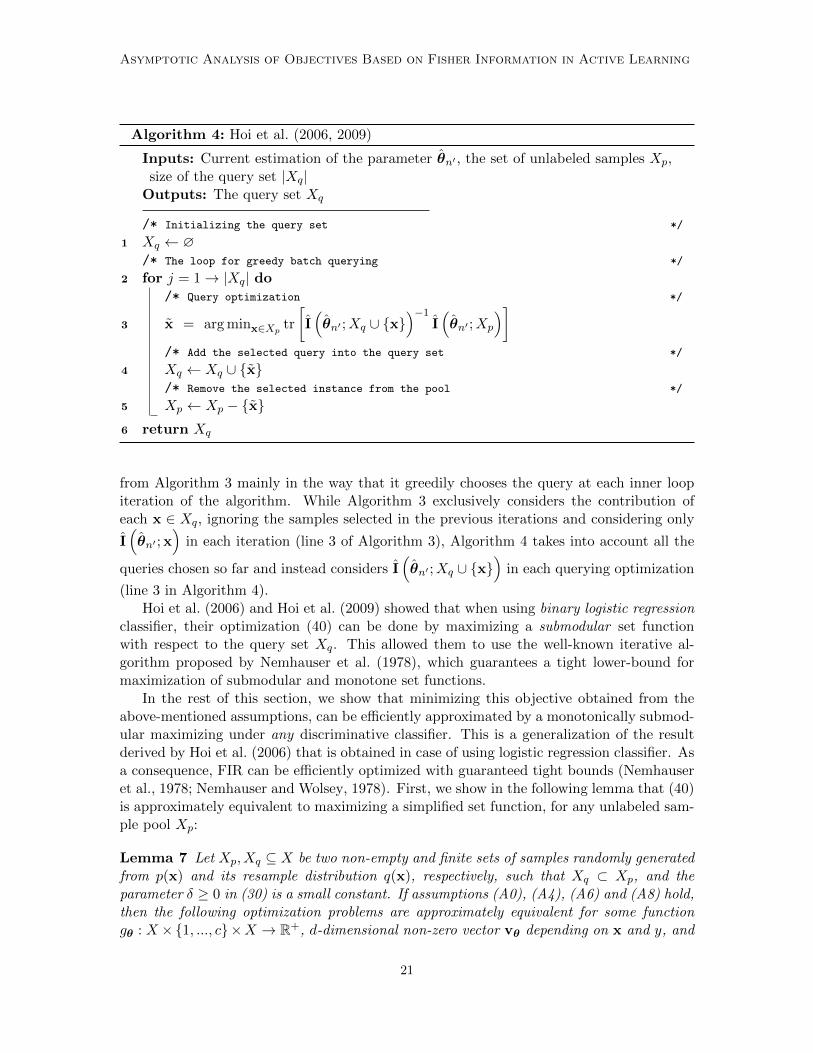
Algorithm 4: Hoi et al. (2006, 2009)
Inputs: Current estimation of the parameter θn′ , the set of unlabeled samples Xp,size of the query set |Xq|
Outputs: The query set Xq
/* Initializing the query set */
1 Xq ← ∅/* The loop for greedy batch querying */
2 for j = 1→ |Xq| do/* Query optimization */
3 x = arg minx∈Xptr
[I(θn′ ;Xq ∪ x
)−1I(θn′ ;Xp
)]/* Add the selected query into the query set */
4 Xq ← Xq ∪ x/* Remove the selected instance from the pool */
5 Xp ← Xp − x6 return Xq
from Algorithm 3 mainly in the way that it greedily chooses the query at each inner loopiteration of the algorithm. While Algorithm 3 exclusively considers the contribution ofeach x ∈ Xq, ignoring the samples selected in the previous iterations and considering only
I(θn′ ; x
)in each iteration (line 3 of Algorithm 3), Algorithm 4 takes into account all the
queries chosen so far and instead considers I(θn′ ;Xq ∪ x
)in each querying optimization
(line 3 in Algorithm 4).Hoi et al. (2006) and Hoi et al. (2009) showed that when using binary logistic regression
classifier, their optimization (40) can be done by maximizing a submodular set functionwith respect to the query set Xq. This allowed them to use the well-known iterative al-gorithm proposed by Nemhauser et al. (1978), which guarantees a tight lower-bound formaximization of submodular and monotone set functions.
In the rest of this section, we show that minimizing this objective obtained from theabove-mentioned assumptions, can be efficiently approximated by a monotonically submod-ular maximizing under any discriminative classifier. This is a generalization of the resultderived by Hoi et al. (2006) that is obtained in case of using logistic regression classifier. Asa consequence, FIR can be efficiently optimized with guaranteed tight bounds (Nemhauseret al., 1978; Nemhauser and Wolsey, 1978). First, we show in the following lemma that (40)is approximately equivalent to maximizing a simplified set function, for any unlabeled sam-ple pool Xp:
Lemma 7 Let Xp, Xq ⊆ X be two non-empty and finite sets of samples randomly generatedfrom p(x) and its resample distribution q(x), respectively, such that Xq ⊂ Xp, and theparameter δ ≥ 0 in (30) is a small constant. If assumptions (A0), (A4), (A6) and (A8) hold,then the following optimization problems are approximately equivalent for some functiongθ : X ×1, ..., c×X → R+, d-dimensional non-zero vector vθ depending on x and y, and
21

Sourati, Akcakaya, Leen, Erdogmus and Dy
for all θ ∈ Ω :
(i) arg minXq⊂Xp
tr[I(θ;Xq)
−1I(θ;Xp)], (41a)
(ii) arg maxXq⊂Xp
∑x∈Xp−Xq
c∑y=1
−1
δ · ‖vθ(x, y)‖−2 +∑
x′∈Xqgθ(x, y,x′)
. (41b)
The approximation is more accurate for smaller δ and well-conditioned Monte-Carlo ap-proximation of proposal Fisher information matrix.
The proof can be found in Appendix C. Note that Lemma 7, as stated above, does notdepend on the size of Xq. However, just as before, in practice it is usually assumed that|Xq| > 0 is fixed and therefore the optimizations in (41) should be considered with car-dinality constraint. In general, combinatorial maximization problems can turn out to beintractable. Next, it is shown that the objective at hand is a monotonically submodular setfunction in terms of Xq and therefore can be maximized efficiently with a greedy approachsuch as that shown in Algorithm 4.
Theorem 8 Suppose fθ : 2Xp → R is defined as
fθ(Xq) =∑
x∈Xp−Xq
c∑y=1
−1
δ · ‖vθ(x, y)‖−2 +∑
x′∈Xqgθ(x, y,x′)
, ∀Xq ⊆ Xp, (42)
with vθ a d-dimensional vector depending on x and y, and gθ defined in (91). Then fθ isa submodular and monotone (non-decreasing) set function for all θ ∈ Ω.
The proof is in Appendix D. The result above, together with Lemma 7, imply that the objec-tive of (41b) is a monotonically increasing set function with respect to Xq. Below we presentthe main result that guarantees tight bounds for greedy maximization of monotonic sub-modular set functions. Details of this result, which is also shown to be the optimally efficientsolution to submodular maximization, can be found in the seminal papers by Nemhauseret al. (1978) and Nemhauser and Wolsey (1978).
Theorem 9 (Nemhauser et al. (1978)) Let fθ : 2Xp → R be any submodular and non-decreasing set function with f(∅) = 0 satisfied.8 If Xq is the output of a greedy maximizationalgorithm, and X∗q is the optimal maximizer of fθ with a cardinality constraint (fixed |Xq|),then we have
fθ(Xq) ≥
[1−
(|Xq| − 1
|Xq|
)|Xq |]fθ(X∗q ) ≥
(1− 1
e
)fθ(X∗q ). (43)
In Algorithm 4, the inner loop (lines 2 to 5) implements the minimization in (40) greedily.We have seen above that this set minimization is approximately equivalent to maximizinga submodular and monotone set maximization, which, in turn, is shown to be efficient.
8. This can always be assumed since maximizing a general set function f(Xq) is equivalent to maximizingits adjusted version g(Xq) := f(Xq)− f(∅), which satisfies g(∅) = 0.
22

Asymptotic Analysis of Objectives Based on Fisher Information in Active Learning
Algorithm 5 (Chaudhuri et al., 2015b)
This algorithm uses FIR for doing a probabilistic pool-based active learning. It hasextra assumptions in comparison to our general framework, which are briefly explained inSection 5.1.1. Note that these assumptions are to be made as well as those listed in Section 2.In such settings, Chaudhuri et al. (2015b) gave a finite-sample theoretical analysis for FIRwhen applied to pool-based active learning.
More specifically, suppose p(x) is a uniform PMF and q(x) is a general PMF, bothdefined over the pool Xp. Using the notations in (25), the training Fisher information can
be written as Iq(θn′) =∑
x∈Xpq(x) I(θn′ ,x). Now, assuming that Ip(θn′) has a singular
decomposition of the form∑d
j=1 σjuju>j , FIR can be written as
tr
[Iq(θn′)
−1 Ip(θn′)
]=
d∑j=1
σjtr
[Iq(θn′)
−1uju>j
]
=
d∑j=1
σju>j Iq(θn′)
−1uj . (44)
Minimizing the last term in (44) with respect to PMF q(x)|x ∈ Xp is equivalent to asemidefinite programming after introducing a set of auxiliary variables tj , j =, 1..., d andapplying Schur complements (Vandenberghe and Boyd, 1996):
arg minq(x),x∈Xp
d∑j=1
σjtj (45)
such that
[tj u>juj
∑x∈Xp
q(x) I(θn′ ,x)
] 0,∑
x∈Xp
q(x) = 1.
The steps for this querying method is shown in Algorithm 5. Note that the solution to (45) isslightly modified by mixing it with the uniform distribution over the pool. Such modificationis mainly to establish their theoretical derivations. The mixing coefficient, 0 ≤ λ ≤ 1,reciprocally depends on the number of queries. More specifically, Chaudhuri et al. (2015b)made it equal to 1 − 1
|Xq |1/6. That is, as the number of queries increases, λ shrinks and so
does the modification. Furthermore, in their analysis, they assumed that sampling fromq(x) (line 3 of Algorithm 5) is done with replacement. That is, label of a given sample mightbe queried multiple times.
5.2.1 Comparison with Other Information-theoretic Objectives
In the last part of this section, we compare FIR and two other common querying objectivesfrom the field of information theory. Entropy of class labels and mutual information betweenlabeled and unlabeled samples are two other common active learning objectives. Their goalis mainly to get the largest possible amount of information about class labels of unlabeledsamples from each querying iteration, hence naturally pool-based.
23

Sourati, Akcakaya, Leen, Erdogmus and Dy
Algorithm 5: Chaudhuri et al. (2015b)
Inputs: Current estimation of the parameter θn′ , the set of unlabeled samples Xp,size of the query set |Xq|
Outputs: The query set Xq
/* Solving the semidefinite programming */
1 q(x) ← solution to (45)/* Modification of the solution */
2 q(x) ← λq(x) + (1− λ)U(x)/* Sampling with replacement from the modified proposal */
3 xi ∼ q(x) , i = 1, ..., |Xq|4 return Xq =
x1, ...x|Xq |
Algorithm Complexity
Entropy O(|Xp|cd)
Mutual Information O(|Xp| · |Xq| · c|Xq |+1d
)Zhang and Oles (2000) O(|Xp|cd)
Settles and Craven (2008) O(|Xq| · |Xp| · (cd+ d3)
)Hoi et al. (2006, 2009) O
(|Xq| · |Xp| · (cd+ cd|Xq|+ d3)
)Chaudhuri et al. (2015b) O
(d3|Xp|2 + d4|Xp|+ d5
)Table 2: Computational complexity of different querying algorithms
Entropy-based querying, also known as uncertainty sampling, directly measures theuncertainty with respect to class label of each unlabeled sample and query those withhighest uncertainty. It has been widely popular due to its simplicity and effectivenessespecially in sequential active learning. However, it does not consider interaction betweensamples when selecting multiple queries, which can cause querying very similar samples(redundancy). Therefore, uncertainty sampling shows relatively poor performance in batchactive learning. Mutual information, on the other hand, does not suffer from redundancy,however, it requires a much higher computational complexity.
These two objectives directly measure the amount of information each batch can havewith respect to the class labels (hence prediction-based), as opposed to Fisher informa-tion as a measure of information regarding the distribution parameters (hence inference-based). However, there is no guarantee that by minimizing uncertainty of the class labels(or equivalently, choosing queries with highest amount of information about class labels),the prediction accuracy also increases. Whereas, as we showed earlier, FIR upper-boundsthe expected asymptotic variance of a parameter inference loss function. From this pointof view, FIR has a closer relationship with the performance of a classifier.
24

Asymptotic Analysis of Objectives Based on Fisher Information in Active Learning
Table 2 shows computational complexity of the querying objectives. The algorithm byFukumizu (2000) is excluded from this table since it cannot be used in pool-based sampling.Also note that the complexity reported for mutual information is for the case when it isoptimized greedily. Nevertheless, it still contains an exponential term in its complexity.Entropy-based and Zhang and Oles (2000) have the lowest complexity, but in the expenseof introducing redundancy into the batch of queries. Algorithms by Settles and Craven(2008), Hoi et al. (2006, 2009) and Chaudhuri et al. (2015b) become very expensive whend is large, whereas mutual information can easily get intractable for selecting batches ofhigher size (large |Xq|). Observe that algorithm by Hoi et al. (2006, 2009) is more expensivethan Settles and Craven (2008). Recall that despite similarities in appearance, the formerguarantees tight bound for its greedy optimization, whereas the latter does not.
The complexity for the algorithm by Chaudhuri et al. (2015b) is computed assumingthat a barrier method (following path) is used as its numerical optimization (Boyd andVandenberghe, 2004). From Table 2, this algorithm is the only one whose complexityincreases quadratically with size of the pool |Xp|, and therefore can get significantly slowfor huge pools. Furthermore, it does not depend on |Xq| since the optimization in (45) as itsmain source of computations, only depends on |Xp| and d. Furthermore, for this algorithm,
computing I(θn′ ,x) is assumed to cost O(1) for each x ∈ Xp as it is taken to be independentof y.
6. Conclusion
In this paper, we focused on active learning algorithms in classification problems whoseobjectives are based on Fisher information criterion. As the primary result, we showedthe dependency of the variance of the asymptotic distribution of log-likelihood ratio on theFisher information of the training distribution. Then, we used this dependency to deriveour novel theoretical contribution by establishing the Fisher information ratio (FIR) as theupper bound of expectation of such asymptotic variance. We also showed that replacing thetrue parameter by the current estimate does not remove such upper-boundedness providedthat the current parameter estimate has been obtained using sufficient number of samples.Moreover, we discussed that several layers of approximations can be employed in practiceto simplify FIR; simplifications, that can usually be avoided in pool-based active learning.Additionally, Monte-Carlo simulations and greedy algorithms can be used to evaluate andoptimize the (simplified) FIR objective, respectively. Using this framework, we can distin-guish the main differences between some of the existing FIR-based querying methods in theclassification context. Such comparative analysis, not only shed light on the assumptionsand simplifications of the existing algorithms, it can also be helpful for finding suitabledirections in developing novel active learning algorithms based on the Fisher informationcriterion.
Finally, we remark that the log-likelihood ratio that is used here as the loss function isan inference-based performance metric. It naturally shows up based on the set of assump-tions that are usually being made in FIR-based querying frameworks. The final goal of aclassifier in machine learning is to predict labels of test samples as accurately as possibleand therefore, arguably, prediction-based metrics such as 0/1 loss function better evaluatethe performance of a classifier. While analyzing such metrics was out of scope of this paper,
25

Sourati, Akcakaya, Leen, Erdogmus and Dy
analysis and development of querying algorithms using prediction-based metrics is definitelyan exciting future research direction.
Acknowledgments
This work is primarily supported by NSF IIS-1118061. In addition, Todd Leen was sup-ported under NSF 1258633, 1355603, and 1454956; Deniz Erdogmus was supported by NSFIIS-1149570, CNS-1136027 and SMA-0835976; and Jennifery Dy was also supported by NSFIIS 0915910 and NIH R01HL089856.
Appendix A. Statistical Background
Asymptotic analysis plays an important role in statistics. It considers extreme cases wherethe number of observations is increased with no bounds. In such scenarios, discussionson different notions of convergence of the sequence of random variables naturally arise.Generally speaking, there are three major types of stochastic convergence: convergence inprobability, convergence in law (distribution) and convergence with high probability (almostsurely). Here, we focus on the two former modes of convergence, discuss two fundamentalresults based on them and formalize our notations regarding parameter estimators. Furtherdetails of the following definitions and results can be found in any standard statisticaltextbook such as Lehmann and Casella (1998).
A.1 Convergence of Sequence of Random Variables
Throughout this section, θ1,θ2, ...,θn, ..., denoted simply by θn, is a sequence of mul-tivariate random variables lying in Ω ⊆ Rd. Also suppose that θ0 is a constant vector andθ is another random variable in the same space Ω.
Definition 10 We say that the sequence θn converges in probability to θ0 and write
θnP→ θ0, iff for every ε > 0 we have
P (|θni − θ0i| > ε) → 0, for all i = 1, ..., d, (46)
where θni is the i’th component of θn.
Convergence in probability is invariant with respect to any continuous mapping:
Proposition 11 (Brockwell and Davis 1991, Proposition 6.1.4) If θnP→ θ0 and g :
Ω→ R is a continuous function, then g(θn)P→ g(θ0).
Definition 12 We say that a sequence θn converges in law (in distribution) to the ran-
dom variable θ and write θnL→ θ, iff the sequence of their joint CDFs, Fn, point-wise
converges to the joint CDF of θ:
Fn(a) = P (θn1 ≤ a1, ..., θnd ≤ ad) → F (a) = P (θ1 ≤ a1, ..., θd ≤ ad) ∀a ∈ CF ⊆ Rd,(47)
where CF is the set of continuity points of the CDF F .
26
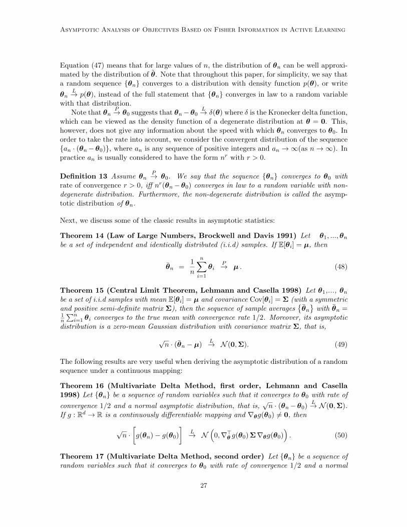
Asymptotic Analysis of Objectives Based on Fisher Information in Active Learning
Equation (47) means that for large values of n, the distribution of θn can be well approxi-mated by the distribution of θ. Note that throughout this paper, for simplicity, we say thata random sequence θn converges to a distribution with density function p(θ), or write
θnL→ p(θ), instead of the full statement that θn converges in law to a random variable
with that distribution.Note that θn
P→ θ0 suggests that θn−θ0L→ δ(θ) where δ is the Kronecker delta function,
which can be viewed as the density function of a degenerate distribution at θ = 0. This,however, does not give any information about the speed with which θn converges to θ0. Inorder to take the rate into account, we consider the convergent distribution of the sequencean · (θn−θ0), where an is any sequence of positive integers and an →∞(as n→∞). Inpractice an is usually considered to have the form nr with r > 0.
Definition 13 Assume θnP→ θ0. We say that the sequence θn converges to θ0 with
rate of convergence r > 0, iff nr(θn−θ0) converges in law to a random variable with non-degenerate distribution. Furthermore, the non-degenerate distribution is called the asymp-totic distribution of θn.
Next, we discuss some of the classic results in asymptotic statistics:
Theorem 14 (Law of Large Numbers, Brockwell and Davis 1991) Let θ1, ...,θnbe a set of independent and identically distributed (i.i.d) samples. If E[θi] = µ, then
θn =1
n
n∑i=1
θiP→ µ . (48)
Theorem 15 (Central Limit Theorem, Lehmann and Casella 1998) Let θ1,..., θnbe a set of i.i.d samples with mean E[θi] = µ and covariance Cov[θi] = Σ (with a symmetricand positive semi-definite matrix Σ), then the sequence of sample averages
θn
with θn =1n
∑ni=1 θi converges to the true mean with convergence rate 1/2. Moreover, its asymptotic
distribution is a zero-mean Gaussian distribution with covariance matrix Σ, that is,
√n · (θn − µ)
L→ N (0,Σ). (49)
The following results are very useful when deriving the asymptotic distribution of a randomsequence under a continuous mapping:
Theorem 16 (Multivariate Delta Method, first order, Lehmann and Casella1998) Let θn be a sequence of random variables such that it converges to θ0 with rate of
convergence 1/2 and a normal asymptotic distribution, that is,√n · (θn−θ0)
L→ N (0,Σ).If g : Rd → R is a continuously differentiable mapping and ∇θg(θ0) 6= 0, then
√n ·[g(θn)− g(θ0)
]L→ N
(0,∇>θ g(θ0) Σ∇θg(θ0)
). (50)
Theorem 17 (Multivariate Delta Method, second order) Let θn be a sequence ofrandom variables such that it converges to θ0 with rate of convergence 1/2 and a normal
27

Sourati, Akcakaya, Leen, Erdogmus and Dy
asymptotic distribution, that is,√n · (θn−θ0)
L→ N (0,Σ). If g : Rd → R is a continuouslydifferentiable mapping where ∇θg(θ0) = 0 and ∇2
θg(θ0) is non-singular in a neighborhood ofθ0, then the sequence g(θn)−g(θ0) converges in law to a mixture of random variables withdegree-one Chi-square distributions, and the rate of convergence is one. More specifically,
n ·[g(θn)− g(θ0)
]L→
d∑i=1
λiχ21, (51)
where λi’s are eigenvalues of Σ1/2∇θg(θ0) Σ1/2. Moreover, variance of this asymptoticdistribution can be written as
1
2
∥∥∥Σ1/2∇2xg(x0) Σ1/2
∥∥∥2F, (52)
where ‖ · ‖F is the Frobenius norm.
Proof For proof see Appendix B.
A.2 Parameter Estimation
Now suppose that the set of independent and identically distributed (i.i.d) set of samplesx1, ...xn are generated from an underlying distribution that belongs to a parametric family,for which the density function p(x |θ) can be represented by a multivariate parameter vectorθ. Assume the true parameter is θ0, that is xi ∼ p(x |θ0), i = 1, ..., n. An estimatorθn = θ(x1, ...,xn) is a function that maps the observed random variables to a point in theparameter space Ω. The subscript n in θn indicates its dependence on the sample size.Since the observations are generated randomly, the estimators are also random and thusθn can be viewed as a sequence of random variables. There are some reserved terms forsuch a sequence, which we introduce in the remaining of this section:
Definition 18 (Consistency) We say that an estimator θn is consistent iff θnP→ θ0.
Based on Theorem 14, sample average of the observation set is a consistent estimator of thetrue mean of the samples. Another important characteristic of estimators is based on thefollowing bound over their covariance matrices:
Theorem 19 (Cramer-Rao, Lehmann and Casella 1998) Let x1, ...,xn ∼ p(x |θ0)and θn = θ(x1, ...,xn) be an estimator. If the first moment of θn is differentiable withrespect to the parameter vector and its second moment is finite, then the following inequal-ity holds for every θ ∈ Ω:
Cov[θn] − (∇θE[θn])> I(θ)−1∇θE[θn]. (53)
The right-hand-side of (53) is called the Cramer-Rao bound of the estimator, where themiddle term is the inverse of the Fisher information matrix of the parametric distributionp(x |θ), defined as
I(θ) := E[∇θ log p(x |θ) · ∇>θ log p(x |θ)
].
28

Asymptotic Analysis of Objectives Based on Fisher Information in Active Learning
Theorem 19 suggests that for an unbiased estimator θn, the inequality over the covariancematrix becomes: Cov[θn] I(θ)−1, ∀θ ∈ Ω.
Definition 20 (Efficiency) We say that an estimator θn is efficient, iff it attains theCramer-Rao bound, meaning that Cov[θn] achieves the lower-bound in (53) for every n =1, 2, ... . Furthermore, we say that θn is asymptotically efficient, iff the lower bound isattained asymptotically (when n→∞).
Appendix B. Proof of Second-order Multivariate Delta Method
In order to prove this theorem, we have to formulate the statistical Taylor expansion. This,in turn, needs a brief introduction of stochastic order notations.
B.1 Stochastic Order Notations
The stochastic order notations are denoted by op and Op, where the former is equivalent toconvergence in probability (Definition 10) and the latter implies boundedness in probability.In what follows, if otherwise stated, θn is a sequence of multivariate random variableslying in Ω ⊆ Rd and an is a sequence of strictly positive real numbers. The skipped proofscan be found in many textbooks on asymptotic theory, such as Brockwell and Davis (1991,Chapter 6).
Definition 21 We write θn = op(an) iff
θinan
= op(1), for all i = 1, ..., d (54)
Definition 22 We write θn = Op(an) iff the sequenceθinan
is bounded in probability for
every i = 1, ..., d, that is, for every ε > 0 there exists δε such that
P
(∣∣∣∣θinan∣∣∣∣ > δε
)< ε, n = 1, 2, ... (55)
We also need the following propositions:
Proposition 23 (Brockwell and Davis, 1991) Let θn and ηn be two sequences ofscalar random variables, and an and bn be two sequences of positive real numbers. Ifθn = Op(an) and ηn = op(bn), then
(i) θ2n = Op(a2n)
(ii) θnηn = op(anbn)
Proposition 24 The followings are true:9
(i) θn = op(an) ⇔ ‖θn ‖ = op(an).
(ii) θn = Op(an) ⇔ ‖θn ‖ = Op(an).
9. Unless subscripted otherwise, ‖ · ‖ denotes the L2 norm in all the equations.
29

Sourati, Akcakaya, Leen, Erdogmus and Dy
Proof The proof of part (i) can be found in Brockwell and Davis (1991, Proposition 6.1.2).Here, we only prove part (ii):
(ii,⇒) : Since θn = Op(an), for every ε > 0 and for every i = 1, ..., d, there exists acoefficient δi > 0 such that
P (|θni| > an · δi) <ε
d, n = 1, 2, .... (56)
Define δmax = maxδ1, ..., δd and note that we can writeθn :
d∑i=1
|θni|2 > (d · an · δmax)2⊆
[d⋂i=1
θn : |θni| ≤ an · δmax
]c
=d⋃i=1
θn : |θni| > an · δmax , (57)
implying that
P(‖θn ‖2 > (d · an · δmax)2
)≤ P
(d⋃i=1
θn : |θni| > an · δmax
)
≤d∑i=1
P (|θni| > an · δmax). (58)
Furthermore, for every i ∈ 1, ..., d, we have δmax ≥ δi. Consequently, the interval(anδmax,∞) is a subset of (anδi,∞) and P (|θni| > anδmax) ≤ P (|θni| > anδi). This impliesthat
P(‖θn ‖2 > (d · an · δmax)2
)≤
d∑i=1
P (|θni| > an · δi) < ε. (59)
Therefore, for every ε > 0, we can choose δε = d · δmax such that P(‖θn ‖an
> δε
)< ε for
every n = 1, 2, .... Therefore, by definition, ‖θn ‖ = Op(an).(ii,⇐) : Suppose ‖θn ‖ = Op(an), that is for every ε > 0 we can find δε > 0 such that
P (‖θn ‖ > an · δε) < ε , n = 1, 2, ... (60)
It is clear that for any given i ∈ 1, ..., d we have
θn : |θni| > an · δε ⊆ θn : ‖θn ‖ > an · δε , (61)
henceP (|θni| > an · δε) ≤ P (‖θn ‖ > an · δε) < ε , n = 1, 2, ... (62)
meaning that θni = Op(an),∀i ∈ 1, ..., d, or equivalently θn = Op(an).
Proposition 25 If θn = Op(an) and an → 0(as n→∞), then θn = op(1).
30

Asymptotic Analysis of Objectives Based on Fisher Information in Active Learning
Proof The goal is to show θn = op(1) or equivalently ‖θn ‖ = op(1) by proving thatP (‖θn ‖ > ε) → 0(as n → ∞) for every ε > 0. Fix ε to a positive real number. In orderto have the sequence of probability numbers P (‖θn ‖ > ε) converging to zero, for everyε0 > 0 there should exist a positive integer N > 0 such that
P (‖θn ‖ > ε) < ε0 ∀n > N. (63)
Because of the assumption of being bounded by an, that is θn = Op(an) or equivalently‖θn ‖ = Op(an), we can choose a real number δ0 > 0 such that
P (‖θn ‖ > anδ0) < ε0 n = 1, 2, ... (64)
On the other hand, since an → 0(as n → ∞), there exists a large enough number N0 > 0such that 0 < an <
εδ0
for all n > N0. Therefore, we get
[0, anδ0] ⊆ [0, ε] ∀n > N0, (65)
implying thatP (‖θn ‖ ≤ anδ0) ≤ P (‖θn ‖ ≤ ε) ∀n > N0. (66)
From inequalities (64) and (66), and noticing that the latter holds for all n whereas theformer is satisfied when n > N0, one can write:
P (‖θn ‖ > ε) ≤ P (‖θn ‖ > anδ0) < ε0 ∀n > N0. (67)
Therefore, for every ε0 > 0, equation (63) is guaranteed if N is chosen to be equal to N0
so that inequality (66) is satisfied. Similarly, this can be written for every ε > 0, thus theproof is complete.
Proposition 26 (Serfling 2002, Chapter 1) Let θn be a sequence of random vari-
ables. If there exists a random variable θ such that θnL→ θ, then θn = Op(1).
B.2 Second-order Statistical Taylor Expansion
Now we are ready to establish the second-order statistical Taylor expansion.
Theorem 27 Let θn be a sequence of random vectors in a convex and compact set Ω ⊆ Rdand θ0 ∈ Ω be a constant vector such that θn−θ0 = Op(an) where an → 0(as n → ∞). Ifg : Ω→ R is a C3 function , then
g(θn) = g(θ0) + ∇>θ g(θ0)(θn−θ0) +1
2(θn−θ0)
>∇2θg(θ0)(θn−θ0) + op(a
2n).
(68)
Proof Since g is twice continuously differentiable in a neighborhood of θ0, it can be writtenin terms of the Taylor expansion as
g(θ) = g(θ0) + (θ−θ0)>∇θg(θ0) +
1
2(θ−θ0)
>∇2θg(θ0)(θ−θ0) + r2(θ,θ0), (69)
31

Sourati, Akcakaya, Leen, Erdogmus and Dy
where r2(θ,θ0) is the Lagrange remainder of second order. Based on Taylor’s polynomialtheorem for multivariate functions, there exists a number t ∈ [0, 1] such that θ∗ = tθ +(1−t)θ0 ∈ Ω (due to convexity of Ω) and
r2(θ,θ0) =1
6
∑1≤i,j,k≤d
∂3g(θ∗)
∂θi∂θj∂θk(θi − θ0i)(θj − θ0j)(θk − θ0k). (70)
But since Ω is compact and g ∈ C3, the third derivative of g is bounded10 and thereforethere exists M > 0 such that∣∣∣∣ ∂3g(θ)
∂θi∂θj∂θk
∣∣∣∣ ≤ M ,∀θ ∈ Ω ,∀i, j, k ∈ 1, ..., d. (71)
Hence, the Lagrange remainder can be bounded by
|r2(θ,θ0)| ≤M
6
∑1≤i,j,k≤3
|θi − θ0i| · |θj − θ0j | · |θk − θ0k|
=M
6‖θ−θ0 ‖31
≤ M ′
6‖θ−θ0 ‖3, (72)
where M ′ = cuM and cu is obtained from the equivalence of norms in Rd vector space.11
Now define the function h : Ω→ R as below
h(θ) :=
r2(θ,θ0)
‖θ−θ0 ‖2/2,θ 6= θ0
0 ,θ = θ0
(74)
Note that h(θ) is continuous at θ = θ0: due to boundedness of r2(θ,θ0), h(θ) is alsobounded by
|h(θ)| ≤ M ′
3‖θ−θ0 ‖. (75)
Hence, for every ε > 0, we can select δε = 3εM ′ such that the following continuity condition
holds:
‖θ−θ0 ‖ < δε ⇒ |h(θ)| ≤ ε. (76)
10. This is because of the following Theorem in real analysis:
Theorem 28 Let X and Y be two vector spaces. If g : X → Y is continuous and X is compact, thenf(X) is compact in Y .
In special case of this theorem, where Y = R, compactness of f(X) is equivalent to boundedness andclosedness.
11. Two norm functions ‖ · ‖(1) and ‖ · ‖(2) in a vector space Ω, are called equivalent iff there exist constantscu ≥ cd > 0 such that
cd‖θ ‖(2) ≤ ‖θ ‖(1) ≤ cu‖θ ‖(2) , ∀θ ∈ Ω. (73)
32

Asymptotic Analysis of Objectives Based on Fisher Information in Active Learning
Continuity of h(θ) at θ = θ0 implies limθ→θ0 h(θ) = h(θ0) = 0. Furthermore, sinceθn−θ0 = Op(an) and an → 0(as n → ∞), Proposition 25 suggests that θn−θ0 = op(1).These two enable us to use Proposition 11 and write
h(θn)− h(θ0) = h(θn) = op(1). (77)
Finally, from equation (74) and Propositions 23, 24 and 25, we can write that
r2(θn,θ0) = h(θn) · ‖θn−θ0 ‖2
2= op(1) ·Op(a2n) = op(a
2n) (78)
B.3 Second-order Multivariate Delta Method
Finally, here is the proof of second-order multivariate Delta method (Theorem 17):
Proof From the assumption for convergence in law, i.e.,√n(θn−θ0)
L→ N (0,Σ), and
Proposition 26, one concludes that√n(θn−θ0) = Op(1) and therefore θn−θ0 = Op
(1√n
).
Thus, we can use Theorem 27 with an = 1√n
to write
g(θ) = g(θ0) + (θ−θ0)>∇θg(θ0) +
1
2(θ−θ0)
>∇2θg(θ0)(θ−θ0) + op
(1
n
), (79)
hence
n
[g(θ)− g(θ0)
]=
1
2
[√n · (θ−θ0)
]>∇2θg(θ0)
[√n · (θ−θ0)
]+ op(1)
L→ 1
2N (0,Σ)>∇2
θg(θ0)N (0,Σ)
=1
2N (0, Id)>
[Σ1/2∇2
θg(θ0) Σ1/2]N (0, Id). (80)
Define Γ := Σ1/2∇2θg(θ0) Σ1/2 and rewrite the right-hand-side element-wise as
1
2N (0, Id)>ΓN (0, Id) =
1
2
d∑i=1
λiN (0, 1)2 =1
2
d∑i=1
λiχ21, (81)
where λi’s are eigenvalues of Γ. Finally, noting that the terms in the Chi-square mixtureare independent, variance of the convergent random variable can be easily computed as
Var
[1
2
d∑i=1
λiχ21
]=
1
4
d∑i=1
λ2i ·Var[χ21
]=
1
2
d∑i=1
λ2i
=1
2
∥∥∥Σ1/2∇2xg(x0) Σ1/2
∥∥∥2F. (82)
33

Sourati, Akcakaya, Leen, Erdogmus and Dy
Appendix C. Proof of Lemma 7
We first substitute the score function of the classifier, i.e.,
∇θ log p(y|x,θ) =∇θp(y|x,θ)
p(y|x,θ),
into Monte-Carlo approximation of Iq to get
I(θ;Xq) =1
|Xq|∑x∈Xq
c∑y=1
p(y|x,θ) ·∇θp(y|x,θ)∇>θ p(y|x,θ)
p(y|x,θ)2+ δId
=1
|Xq|∑x∈Xq
c∑y=1
∇θp(y|x,θ).∇>θ p(y|x,θ)
p(y|x,θ)+ δId. (83)
Define the vector vθ(x, y) := ∇θp(y|x,θ)
/√p(y|x,θ) and rewrite I(θ;Xq) as
I(θ;Xq) =1
|Xq|∑x∈Xq
c∑y=1
vθ(x, y).vθ(x, y)> + δ · Id. (84)
On the other hand, since Xq ⊂ Xp we can write I(θ;Xp) in terms of I(θ;Xq) by breakingthe summation over Xp into summations over Xq and Xp −Xq as follows:
I(θ;Xp) =|Xq||Xp|
1
|Xq|∑x∈Xq
c∑y=1
vθ(x, y).vθ(x, y)> + δ · Id
+
1
|Xp|∑
x∈Xp−Xq
c∑y=1
vθ(x, y).vθ(x, y)> + δ
(|Xp| − |Xq||Xp|
)· Id
=
(|Xq||Xp|
)· I(θ;Xq) +
1
|Xp|∑
x∈Xp−Xq
c∑y=1
vθ(x, y).vθ(x, y)>
+ δ
(|Xp| − |Xq||Xp|
)· Id (85)
Now that we related the Fisher information matrices to each other, we can compute theproduct of I(θ;Xp) and I(θ;Xq)
−1 as
I(θ;Xq)−1I(θ;Xp) =
(|Xq||Xp|
)· Id +
I(θ;Xq)−1
|Xp|
∑x∈Xp−Xq
c∑y=1
vθ(x, y) · vθ(x, y)>
+ δ
(|Xp| − |Xq||Xp|
)· I(θ;Xq)
−1. (86)
34
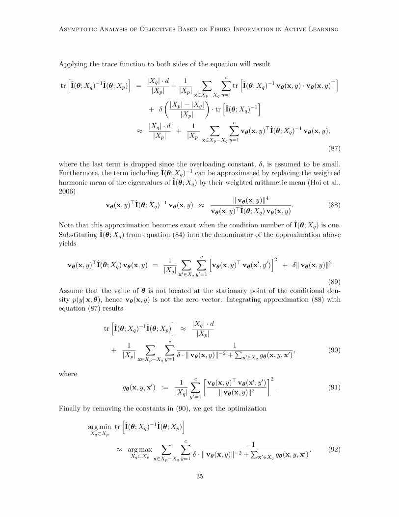
Asymptotic Analysis of Objectives Based on Fisher Information in Active Learning
Applying the trace function to both sides of the equation will result
tr[I(θ;Xq)
−1I(θ;Xp)]
=|Xq| · d|Xp|
+1
|Xp|∑
x∈Xp−Xq
c∑y=1
tr[I(θ;Xq)
−1 vθ(x, y) · vθ(x, y)>]
+ δ
(|Xp| − |Xq||Xp|
)· tr[I(θ;Xq)
−1]
≈ |Xq| · d|Xp|
+1
|Xp|∑
x∈Xp−Xq
c∑y=1
vθ(x, y)>I(θ;Xq)−1 vθ(x, y),
(87)
where the last term is dropped since the overloading constant, δ, is assumed to be small.Furthermore, the term including I(θ;Xq)
−1 can be approximated by replacing the weighted
harmonic mean of the eigenvalues of I(θ;Xq) by their weighted arithmetic mean (Hoi et al.,2006)
vθ(x, y)>I(θ;Xq)−1 vθ(x, y) ≈ ‖vθ(x, y)‖4
vθ(x, y)>I(θ;Xq) vθ(x, y). (88)
Note that this approximation becomes exact when the condition number of I(θ;Xq) is one.
Substituting I(θ;Xq) from equation (84) into the denominator of the approximation aboveyields
vθ(x, y)>I(θ;Xq) vθ(x, y) =1
|Xq|∑
x′∈Xq
c∑y′=1
[vθ(x, y)> vθ(x′, y′)
]2+ δ‖vθ(x, y)‖2
(89)Assume that the value of θ is not located at the stationary point of the conditional den-sity p(y|x,θ), hence vθ(x, y) is not the zero vector. Integrating approximation (88) withequation (87) results
tr[I(θ;Xq)
−1I(θ;Xp)]≈ |Xq| · d
|Xp|
+1
|Xp|∑
x∈Xp−Xq
c∑y=1
1
δ · ‖vθ(x, y)‖−2 +∑
x′∈Xqgθ(x, y,x′)
, (90)
where
gθ(x, y,x′) :=1
|Xq|
c∑y′=1
[vθ(x, y)> vθ(x′, y′)
‖vθ(x, y)‖2
]2. (91)
Finally by removing the constants in (90), we get the optimization
arg minXq⊂Xp
tr[I(θ;Xq)
−1I(θ;Xp)]
≈ arg maxXq⊂Xp
∑x∈Xp−Xq
c∑y=1
−1
δ · ‖vθ(x, y)‖−2 +∑
x′∈Xqgθ(x, y,x′)
. (92)
35

Sourati, Akcakaya, Leen, Erdogmus and Dy
Appendix D. Proof of Theorem 8
Proof of this Theorem is a generalization of the discussion by Hoi et al. (2006), with clari-fication of all the assumptions and approximations made.
First, note that the function fθ can be broken into simpler terms fθ(Xq) =∑c
y=1 fθ(Xq;y), where
fθ(Xq; y) =∑
x∈Xp−Xq
−1
δ · ‖vθ(x, y)‖−2 +∑
x′∈Xqgθ(x, y,x′)
, ∀Xq ⊆ Xp. (93)
Therefore, in order to prove submodularity and monotonicity of fθ, it suffices to provethese properties for fθ(·; y) for all y ∈ 1, ..., c. Fix y and take any subset Xq ⊆ Xp andξ ∈ Xp −Xq. Then, we can write
fθ(Xq ∪ ξ; y) =∑
x∈Xp−(Xq∪ξ)
−1
δ · ‖vθ(x, y)‖−2 +∑
x′∈Xq∪ξ gθ(x, y,x′)
=∑
x∈Xp−Xq
−1
δ · ‖vθ(x, y)‖−2 +∑
x′∈Xq∪ξ gθ(x, y,x′)
+1
δ · ‖vθ(ξ, y)‖−2 +∑
x′∈Xq∪ξ gθ(ξ, y,x′).
We then form the discrete derivative of fθ(·; y) at Xq to get
ρfθ(·;y)(Xq; ξ) = fθ(Xq ∪ ξ; y) − fθ(Xq; y)
=∑
x∈Xp−Xq
[−1
δ‖vθ(x,y)‖2
+∑
x′∈Xq∪ξ gθ(x, y,x′)+
1δ
‖vθ(x,y)‖2+∑
x′∈Xqgθ(x, y,x′)
]
+1
δ‖vθ(x,y)‖2
+∑
x′∈Xq∪ξ gθ(ξ, y,x′).
The right-hand-side can be rewritten as
∑x∈Xp−Xq
gθ(x, y, ξ)(δ
‖vθ(x,y)‖2+∑
x′∈Xq∪ξ gθ(x, y,x′))(
δ‖vθ(x,y)‖2
+∑
x′∈Xqgθ(x, y,x′)
)
+1
δ‖vθ(x,y)‖2
+∑
x′∈Xq∪ξ gθ(ξ, y,x′). (94)
Since by definition gθ(x, y,x′) ≥ 0,∀x, y,x′, all of the terms in (94) are non-negative andtherefore ρfθ(·;y)(Xq; ξ) ≥ 0. This is true for any Xq ⊆ Xp, hence monotonicity of fθ(·; y)is obtained. Now let us take any superset Xq′ such that Xq ⊆ Xq′ ⊆ Xp and ξ ∈ Xp −Xq′ ,and form the difference between their corresponding discrete derivatives. From (94), we will
36

Asymptotic Analysis of Objectives Based on Fisher Information in Active Learning
have
ρfθ(·;y)(Xq; ξ)− ρfθ(·;y)(Xq′ ; ξ)
=∑
x∈Xp−Xq
gθ(x, y, ξ)(δ
‖vθ(x,y)‖2+∑
x′∈Xq∪ξ gθ(x, y,x′))(
δ‖vθ(x,y)‖2
+∑
x′∈Xqgθ(x, y,x′)
)
+1
δ‖vθ(ξ,y)‖2
+∑
x′∈Xq∪ξ gθ(ξ, y,x′)
−∑
x∈Xp−Xq′
gθ(x, y, ξ)(δ
‖vθ(x,y)‖2+∑
x′∈Xq′∪ξgθ(x, y,x′)
)(δ
‖vθ(x,y)‖2+∑
x′∈Xq′gθ(x, y,x′)
)
− 1δ
‖vθ(ξ,y)‖2+∑
x′∈Xq′∪ξgθ(ξ, y,x′)
. (95)
From non-negativity of gθ and that Xq ⊆ Xq′ , we can conclude that for any x ∈ X andy ∈ 1, ..., c, ∑
x′∈Xq′
gθ(x, y,x′) ≥∑
x′∈Xq
gθ(x, y,x′)
⇔
∑x′∈Xq′
gθ(x, y,x′) +δ
‖vθ(x, y)‖2
−1 ≤ ∑x′∈Xq
gθ(x, y,x′) +δ
‖vθ(x, y)‖2
−1
⇔ −
∑x′∈Xq′
gθ(x, y,x′) +δ
‖vθ(x, y)‖2
−1 ≥ −
∑x′∈Xq
gθ(x, y,x′) +δ
‖vθ(x, y)‖2
−1(96)
Similarly, since Xq ∪ ξ ⊆ Xq′ ∪ ξ we will get
−
∑x′∈Xq′∪ξ
gθ(x, y,x′) +δ
‖vθ(x, y)‖2
−1 ≥ − ∑x′∈Xq∪ξ
gθ(x, y,x′) +δ
‖vθ(x, y)‖2
−1(97)
Applying the inequalities (96) and (97) into euqation (95) results
ρfθ(·;y)(Xq; ξ)− ρfθ(·;y)(Xq′ ; ξ)
≥∑
x∈Xp−Xq
gθ(x, y, ξ)(δ
‖vθ(x,y)‖2+∑
x′∈Xq∪ξ gθ(x, y,x′))(
δ‖vθ(x,y)‖2
+∑
x′∈Xqgθ(x, y,x′)
)
−∑
x∈Xp−Xq′
gθ(x, y, ξ)(δ
‖vθ(x,y)‖2+∑
x′∈Xq∪ξ gθ(x, y,x′))(
δ‖vθ(x,y)‖2
+∑
x′∈Xqgθ(x, y,x′)
)
+1
δ‖vθ(ξ,y)‖2
+∑
x′∈Xq∪ξ gθ(ξ, y,x′)− 1
δ‖vθ(ξ,y)‖2
+∑
x′∈Xq∪ξ gθ(ξ, y,x′), (98)
37

Sourati, Akcakaya, Leen, Erdogmus and Dy
which yields12∑x∈Xq′−Xq
gθ(x, y, ξ)(δ
‖vθ(x,y)‖2+∑
x′∈Xq∪ξ gθ(x, y,x′))(
δ‖vθ(x,y)‖2
+∑
x′∈Xqgθ(x, y,x′)
) ≥ 0.
(99)Inequality (99) holds for any Xq ⊆ Xp; hence submodularity of fθ(·; y) stands for all y ∈1, ..., c and θ ∈ Ω.
References
Pranjal Awasthi, Maria Florina Balcan, and Philip M Long. The power of localization forefficiently learning linear separators with noise. arXiv preprint arXiv:1307.8371, 2013.
Javad Azimi, Alan Fern, Xiaoli Zhang-Fern, Glencora Borradaile, and Brent Heeringa.Batch active learning via coordinated matching. arXiv preprint arXiv:1206.6458, 2012.
Maria-Florina Balcan, Alina Beygelzimer, and John Langford. Agnostic active learning.In Proceedings of the 23rd International Conference on Machine Learning, pages 65–72.ACM, 2006.
Alina Beygelzimer, John Langford, Zhang Tong, and Daniel J Hsu. Agnostic active learningwithout constraints. In Advances in Neural Information Processing Systems, pages 199–207, 2010.
Christopher M Bishop. Pattern Recognition and Machine Learning, volume 1. SpringerNew York, 2006.
Stephen Boyd and Lieven Vandenberghe. Convex optimization. Cambridge university press,2004.
Peter J Brockwell and Richard A Davis. Time Series: Theory and Methods. Springer, 1991.
Kamalika Chaudhuri, Sham M Kakade, Praneeth Netrapalli, and Sujay Sanghavi. Con-vergence rates of active learning for maximum likelihood estimation. arXiv preprintarXiv:1506.02348, 2015a.
Kamalika Chaudhuri, Sham M Kakade, Praneeth Netrapalli, and Sujay Sanghavi. Conver-gence rates of active learning for maximum likelihood estimation. In Advances in NeuralInformation Processing Systems, pages 1090–1098, 2015b.
Yuxin Chen and Andreas Krause. Near-optimal batch mode active learning and adap-tive submodular optimization. In Proceedings of The 30th International Conference onMachine Learning, pages 160–168, 2013.
12. The inequality in (98) is obtained by the fact that, for every four positive real numbers a, a0, b and b0,if we have −a ≥ −a0 and −b ≥ −b0 (similar to equations 96 and 97), then
−a · b = (−a) · b ≥ (−a0) · b = a0 · (−b) ≥ a0 · (−b0) = −a0 · b0.
38

Asymptotic Analysis of Objectives Based on Fisher Information in Active Learning
David Cohn, Les Atlas, and Richard Ladner. Improving generalization with active learning.Machine learning, 15(2):201–221, 1994.
David A Cohn. Neural network exploration using optimal experiment design. Neural Net-works, 9(6):1071–1083, 1996.
David A Cohn, Zoubin Ghahramani, and Michael I Jordan. Active learning with statisticalmodels. arXiv preprint cs/9603104, 1996.
Sanjoy Dasgupta. Coarse sample complexity bounds for active learning. In Advances inNeural Information Processing Systems, pages 235–242, 2005.
Sanjoy Dasgupta, Adam Tauman Kalai, and Claire Monteleoni. Analysis of perceptron-based active learning. In Learning Theory, pages 249–263. Springer, 2005.
Sanjoy Dasgupta, Claire Monteleoni, and Daniel J Hsu. A general agnostic active learningalgorithm. In Advances in Neural Information Processing Systems, pages 353–360, 2007.
Richard O Duda, Peter E Hart, and David G Stork. Pattern Classification. John Wiley &Sons,, 1999.
Valerii Vadimovich Fedorov. Theory of Optimal Experiments. Elsevier, 1972.
Yoav Freund, H Sebastian Seung, Eli Shamir, and Naftali Tishby. Selective sampling usingthe query by committee algorithm. Machine Learning, 28(2-3):133–168, 1997.
Yifan Fu, Xingquan Zhu, and Bin Li. A survey on instance selection for active learning.Knowledge and information systems, 35(2):249–283, 2013.
Kenji Fukumizu. Statistical active learning in multilayer perceptrons. IEEE Transactionson Neural Networks, 11(1):17–26, 2000.
Yuhong Guo. Active instance sampling via matrix partition. In Advances in Neural Infor-mation Processing Systems, pages 802–810, 2010.
Yuhong Guo and Russell Greiner. Optimistic active-learning using mutual information. InNational Joint Conferences on Artificial Intelligence, volume 7, pages 823–829, 2007.
Yuhong Guo and Dale Schuurmans. Discriminative batch mode active learning. In Advancesin Neural Information Processing Systems, pages 593–600, 2008.
Steve Hanneke. Activized learning: Transforming passive to active with improved labelcomplexity. Journal of Machine Learning Research, 13(May):1469–1587, 2012.
Steve Hanneke et al. Rates of convergence in active learning. The Annals of Statistics, 39(1):333–361, 2011.
Steven CH Hoi, Rong Jin, Jianke Zhu, and Michael R Lyu. Batch mode active learning andits application to medical image classification. In Proceedings of the 23rd InternationalConference on Machine Learning, pages 417–424. ACM, 2006.
39

Sourati, Akcakaya, Leen, Erdogmus and Dy
Steven CH Hoi, Rong Jin, and Michael R Lyu. Batch mode active learning with applicationsto text categorization and image retrieval. IEEE Transactions on Knowledge and DataEngineering, 21(9):1233–1248, 2009.
Alex Holub, Pietro Perona, and Michael C Burl. Entropy-based active learning for objectrecognition. In IEEE Computer Society Conference on Computer Vision and PatternRecognition, Workshop on Online Learning for Classification, pages 1–8, 2008.
Ming Ji and Jiawei Han. A variance minimization criterion to active learning on graphs. InAISTATS, pages 556–564, 2012.
Andreas Krause, Ajit Singh, and Carlos Guestrin. Near-optimal sensor placements in gaus-sian processes: Theory, efficient algorithms and empirical studies. The Journal of MachineLearning Research, 9:235–284, 2008.
Erich Leo Lehmann and George Casella. Theory of Point Estimation. Springer, 1998.
David MacKay. Information-based objective functions for active data selection. NeuralComputation, 4(4):590–604, 1992.
Noboru Murata, Shuji Yoshizawa, and S-I Amari. Network information criterion-determining the number of hidden units for an artificial neural network model. IEEETransactions on Neural Networks, 5(6):865–872, 1994.
George L Nemhauser and Leonard A Wolsey. Best algorithms for approximating the max-imum of a submodular set function. Mathematics of Operations Research, 3(3):177–188,1978.
George L Nemhauser, Laurence A Wolsey, and Marshall L Fisher. An analysis of approx-imations for maximizing submodular set functionsi. Mathematical Programming, 14(1):265–294, 1978.
Hieu T Nguyen and Arnold Smeulders. Active learning using pre-clustering. In Proceedingsof the 21st International Conference on Machine Learning, page 79. ACM, 2004.
Andrew I Schein and Lyle H Ungar. Active learning for logistic regression: an evaluation.Machine Learning, 68(3):235–265, 2007.
Greg Schohn and David Cohn. Less is more: Active learning with support vector machines.In International Conference on Machine Learning, pages 839–846, 2000.
Robert J Serfling. Approximation Theorems of Mathematical Statistics. John Wiley & Sons,2002.
Burr Settles. Active learning. Synthesis Lectures on Artificial Intelligence and MachineLearning, 6(1):1–114, 2012. doi: 10.2200/S00429ED1V01Y201207AIM018.
Burr Settles and Mark Craven. An analysis of active learning strategies for sequence label-ing tasks. In Proceedings of the Conference on Empirical Methods in Natural LanguageProcessing, pages 1070–1079, 2008.
40

Asymptotic Analysis of Objectives Based on Fisher Information in Active Learning
Burr Settles, Mark Craven, and Soumya Ray. Multiple-instance active learning. In Advancesin Neural Information Processing Systems, pages 1289–1296, 2008.
Hidetoshi Shimodaira. Improving predictive inference under covariate shift by weightingthe log-likelihood function. Journal of Statistical Planning and Inference, 90(2):227–244,2000.
Jamshid Sourati, Murat Akcakaya, Jennifer G Dy, Todd K Leen, and Deniz Erdogmus.Classification active learning based on mutual information. Entropy, 18(2):51, 2016.
Simon Tong and Daphne Koller. Support vector machine active learning with applicationsto text classification. The Journal of Machine Learning Research, 2:45–66, 2002.
Lieven Vandenberghe and Stephen Boyd. Semidefinite programming. SIAM review, 38(1):49–95, 1996.
Larry Wasserman. All of Statistics: A Concise Course in Statistical Inference. Springer,2004.
Xiaojing Yang. A matrix trace inequality. Journal of Mathematical Analysis and Applica-tions, 250(1):372–374, 2000.
Chicheng Zhang and Kamalika Chaudhuri. Beyond disagreement-based agnostic activelearning. In Advances in Neural Information Processing Systems, pages 442–450, 2014.
Tong Zhang and F Oles. The value of unlabeled data for classification problems. In Pro-ceedings of the 17th International Conference on Machine Learning, pages 1191–1198,2000.
Xiaojin Zhu, John Lafferty, and Zoubin Ghahramani. Combining active learning and semi-supervised learning using gaussian fields and harmonic functions. In International Con-ference on Machine Learning, Workshop on the Continuum from Labeled to UnlabeledData in Machine Learning and Data Mining, pages 58–65, 2003.
41