asymmetric solitons in parity-time-symmetric double-hump ... · 2 asymmetric solitons in...

ASYMMETRIC SOLITONS IN PARITY-TIME-SYMMETRIC DOUBLE-HUMPSCARFF-II POTENTIALS

PENGFEI LI1, DUMITRU MIHALACHE2, LU LI1,∗

1Institute of Theoretical Physics, Shanxi University, Taiyuan 030006, ChinaE-mail∗: [email protected]

2Horia Hulubei National Institute of Physics and Nuclear Engineering,Magurele-Bucharest, 077125, Romania

Received February 18, 2016

Symmetric and asymmetric solitons that form in self-focusing optical wave-guides with parity-time (PT )-symmetric double-hump Scarff-II potentials are inves-tigated. It is shown that the branch corresponding to asymmetric solitons bifurcates outfrom the base branch of PT -symmetric solitons with the increasing of the input power.The stability of symmetric and asymmetric stationary solitons is investigated by em-ploying both linear stability analysis and direct numerical simulations. The effects ofthe soliton power, the separation between the two humps of the potential, the width andthe modulation strength of the potential, on the structure of the linear stability eigen-value spectrum is also studied. The different instability scenarios of PT -symmetricsolitons have also been revealed by using direct numerical simulations.

Key words: Bifurcation of eigenvalue spectrum, asymmetric soliton, parity-time-symmetry breaking.

PACS: 42.65.Tg, 03.65.Ge, 11.30.Er.

1. INTRODUCTION

Much attention has been paid in recent years to the study of localized opti-cal waveforms in balanced gain and loss waveguides. These optical waveguides canbe used to investigate subtle quantum concepts by using optical waves for the rea-son of similarity between paraxial optics wave equation and quantum mechanicalSchrodinger equation. One of the key properties is that there exist real eigenvaluespectra in non-Hermitian parity-time (PT )-symmetric Hamiltonian systems [1–3].It it well-known that a necessary condition for a Hamiltonian to be PT -symmetricis U(ξ) = U∗(−ξ), where asterisk denotes the complex conjugation. Thus the PT -symmetry requires that the real part of the complex-valued potential U(ξ) must be aneven function of the position ξ, whereas the imaginary part must be an odd function.

In optical settings, the real and imaginary components of the potential standfor the distribution of refractive index and gain/loss, respectively [4–6]. Thus suchspecially realized optical devices provide a fertile ground for demonstrating experi-mentally the key characteristics of PT -symmetric Hamiltonians [7, 8]. Furthermore,

RJP 61(Nos. 5-6), 1028–1039 (2016) (c) 2016 - v.1.3a*2016.7.20Rom. Journ. Phys., Vol. 61, Nos. 5-6, P. 1028–1039, Bucharest, 2016

2 Asymmetric solitons in parity-time-symmetric double-hump Scarff-II potentials 1029

PT -symmetric soliton solutions and the corresponding beam dynamics have beenalso investigated in nonlinear regimes with complex-valued PT -symmetric poten-tials. Various kinds of optical solitons have been studied, including bright solitons,gap solitons, Bragg solitons, and gray or dark solitons and vortices [9–19]. Theobservation of such PT -symmetric optical solitons is a challenging issue in spiteof a series of theoretical predictions in many optical settings, due to the difficultyof realizing gain/loss and optical nonlinearity in perfect synergy. Recently, stableoptical discrete solitons in PT -symmetric mesh lattices have been experimentallydemonstrated [20]. Unlike other non-conservative nonlinear systems where dissipa-tive solitons appear as fixed points in the parameter space of the governing equations,the discrete PT -symmetric solitons in optical lattices form a continuous parametricfamily of solutions [20]. Also, the observation of Bloch oscillations in complex PT -symmetric photonic lattices has been recently reported [21].

Also, optical solitons in mixed linear-nonlinear lattices, optical lattice solitonsin media described by the complex Ginzburg-Landau model with PT -symmetric pe-riodic potentials, vector solitons in PT -symmetric coupled waveguides, defect soli-tons in PT -symmetric lattices, solitons in chains of PT -invariant dimers, solitons innonlocal media, solitons and breathers in PT -symmetric nonlinear couplers, unidi-rectional optical transport induced by the balanced gain-loss profiles, the nonlinearlyinduced PT transition in photonic systems, and asymmetric optical amplifiers basedon parity-time symmetry have been reported [22–43].

Recently, a family of stable PT -symmetry-breaking solitons with real eigen-value spectra have been found for a special class of PT -symmetric potentialsU (ξ)=g2(ξ)+αg(ξ)+ idg(ξ)/dξ, where g(ξ) is a real and even function and α is a realconstant [44]. For this type of potentials, a precondition of the existence of non-PT -symmetric (asymmetric) solitons is miraculously satisfied [45]. These asymmetricsolitons bifurcate out from the base branch of PT -symmetric solitons when the soli-ton power exceeds a certain threshold.

In this paper, we will study the key features of both symmetric and asymmetricsolitons in PT -symmetric double-hump Scarff-II potentials. The paper is organizedas follows. In Sec. 2, the governing model is introduced. The dependence of thenonlinear propagation constant of both asymmetric and symmetric solitons, on theinput power, the width and the modulation strength of the complex-valued potential,and the separation between its two humps, together with the position of bifurcationpoints of asymmetric solitons from the symmetric ones are presented in Sec. 3. InSec. 4, we analyze systematically the stability of both asymmetric and symmetricstationary solutions and their nonlinear evolution dynamics. Section 5 concludes thepaper.

RJP 61(Nos. 5-6), 1028–1039 (2016) (c) 2016 - v.1.3a*2016.7.20

1030 Pengfei Li, Dumitru Mihalache, Lu Li 3

2. THE GOVERNING MODEL

In the context of the paraxial theory, the optical wave propagation in a Kerrnonlinear planar graded-index waveguide with a balanced gain/loss is governed bythe following (1+1)-dimensional wave equation

i∂ψ

∂z+

1

2k0

∂2ψ

∂x2+k0 [F (x)−n0]

n0ψ+

k0n2n0

|ψ|2ψ = 0, (1)

where ψ(z,x) is the complex envelope function of the optical field, k0 = 2πn0/λ isthe wavenumber with λ and n0 being the wavelength and the background refractiveindex, respectively. Here F (x) = FR(x)+ iFI(x) is a complex function, in whichthe real part is the refractive index distribution and the imaginary part stands for thegain/loss, and n2 is the Kerr nonlinear parameter.

Equation (1) can be rewritten in a dimensionless form

i∂Ψ

∂ζ+∂2Ψ

∂ξ2+U (ξ)Ψ+σ |Ψ|2Ψ= 0, (2)

by introducing the normalized transformationsψ(z,x)= (k0 |n2|LD/n0)−1/2Ψ(ζ,ξ),

ξ = x/w0, and ζ = z/LD. Here LD = 2k0w20 is the diffraction length and σ =

n2/ |n2| = ±1 corresponds to self-focusing (+1) or self-defocusing (−1) Kerr-typenonlinearities, respectively. The complex-valued potential is U(ξ) ≡ V (ξ)+ iW (ξ)with V (ξ) = 2k20w

20[FR(x)−n0]/n0 and W (ξ) = 2k20w

20FI(x)/n0.

For PT -symmetric systems, the real and imaginary components of the com-plex potential are required to be even and odd functions, respectively. In general, suchpotentials cannot support continuous families of non-PT -symmetric solutions [45].However, for a special type of PT -symmetric potentials V (ξ) = g2(ξ)+αg(ξ) andW (ξ) = dg(ξ)/dξ with g(ξ) being an arbitrary real and even function and α beingan arbitrary real constant, it has been shown that stable PT -symmetry-breaking soli-tons can occur [44], where as typical examples, the real functions g(ξ) were taken aslocalized double-hump exponential functions or as periodic functions. Subsequently,these results were also extended to two-dimensional potentials [46, 47].

In this paper, we aim to search for the asymmetric soliton solutions correspond-ing to a PT -symmetric double-hump Scarff-II potential, i.e.,

g (ξ) =W0

[sech

(ξ+ ξ0χ0

)+ sech

(ξ− ξ0χ0

)]. (3)

Here, χ0 and ξ0 are related to the width and the separation between the two humps ofthe potential, respectively, andW0 represents the modulation strength of the complexpotential. Note that, in the PT -symmetric Scarff-II potential with a single-hump, thesymmetric solutions in both nonlinear and linear regimes have been studied in Refs.[9, 48].

RJP 61(Nos. 5-6), 1028–1039 (2016) (c) 2016 - v.1.3a*2016.7.20


-10 -5 0 5 10-0.6

0.0

0.6

1.2

-10 -5 0 5 10

0.0

0.5

1.0

-10 -5 0 5 10

0.0

0.5

1.0

0.5 1.0 1.5 2.0 2.5 3.00.5

1.0

1.5

Potential V

W(a)

(c)

(d)

0.5 1.0 1.5 2.0 2.5 3.0-10

-5

0

5

10

P

(e)

0.5 1.0 1.5 2.0 2.5 3.0-10

-5

0

5

10

P

(f)

P

SS AS

(b)

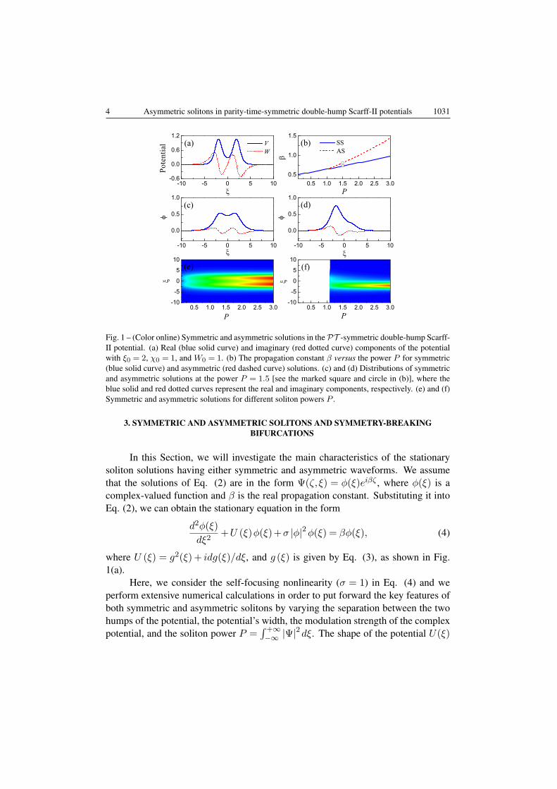
Fig. 1 – (Color online) Symmetric and asymmetric solutions in the PT -symmetric double-hump Scarff-II potential. (a) Real (blue solid curve) and imaginary (red dotted curve) components of the potentialwith ξ0 = 2, χ0 = 1, and W0 = 1. (b) The propagation constant β versus the power P for symmetric(blue solid curve) and asymmetric (red dashed curve) solutions. (c) and (d) Distributions of symmetricand asymmetric solutions at the power P = 1.5 [see the marked square and circle in (b)], where theblue solid and red dotted curves represent the real and imaginary components, respectively. (e) and (f)Symmetric and asymmetric solutions for different soliton powers P .

3. SYMMETRIC AND ASYMMETRIC SOLITONS AND SYMMETRY-BREAKINGBIFURCATIONS

In this Section, we will investigate the main characteristics of the stationarysoliton solutions having either symmetric and asymmetric waveforms. We assumethat the solutions of Eq. (2) are in the form Ψ(ζ,ξ) = ϕ(ξ)eiβζ , where ϕ(ξ) is acomplex-valued function and β is the real propagation constant. Substituting it intoEq. (2), we can obtain the stationary equation in the form

d2ϕ(ξ)

dξ2+U (ξ)ϕ(ξ)+σ |ϕ|2ϕ(ξ) = βϕ(ξ), (4)

where U (ξ) = g2(ξ)+ idg(ξ)/dξ, and g (ξ) is given by Eq. (3), as shown in Fig.1(a).

Here, we consider the self-focusing nonlinearity (σ = 1) in Eq. (4) and weperform extensive numerical calculations in order to put forward the key features ofboth symmetric and asymmetric solitons by varying the separation between the twohumps of the potential, the potential’s width, the modulation strength of the complexpotential, and the soliton power P =

∫ +∞−∞ |Ψ|2 dξ. The shape of the potential U(ξ)

RJP 61(Nos. 5-6), 1028–1039 (2016) (c) 2016 - v.1.3a*2016.7.20


Fig. 2 – (Color online) The nonlinear propagation constant β as a function of the power P for asym-metric (red circles) and symmetric (blue solid spheres) solutions for different (a) separation betweenthe two humps of the potential for the fixed parameters χ0 = 1 and W0 = 1; (b) potential’s width forthe fixed parameters ξ0 = 2 and W0 = 1, and (c) modulation strength of the potential for the fixedparameters χ0 = 1 and ξ0 = 2, respectively. Here, the power P ranges from 0.1 to 3 and σ = 1.

RJP 61(Nos. 5-6), 1028–1039 (2016) (c) 2016 - v.1.3a*2016.7.20


is shown in Fig. 1 (a). The dependence of the propagation constant β on the solitonpower P [the nonlinear dispersion curve β = β(P )] of both symmetric and asymmet-ric soliton solutions is shown in Fig. 1(b), where the blue solid and red dotted curvescorrespond to the symmetric solutions (SS) and the asymmetric solutions (AS), res-pectively. One can see that the stationary solutions in the PT -symmetric potentialare symmetric when P < Pth = 1.1 for our choice of the parameters. However, oncethe power exceeds the threshold value Pth, the asymmetric soliton solution begins tobifurcate out from the symmetric one. It should be emphasized that the asymmet-ric stationary solutions are non-PT -symmetric but their eigenvalues still keep real.Thus, two different kinds of stationary solutions coexist in the region of P ≥ Pth. Wealso find that all of the propagation constants β belonging to the asymmetric solutionsare larger than those of the symmetric ones at equal powers. Similar phenomena ofbifurcation of asymmetric solitons from symmetric ones have been found in differentphysical settings involving Hermitian systems (i.e., without gain and loss); see, forexample Refs. [49–54].

Because Eq. (4) is PT -symmetric, if ϕ(ξ) is a solution, so is ϕ∗(−ξ). Thus, thesymmetric solutions of Eq. (4) satisfy naturally ϕ(ξ) = ϕ∗(−ξ) due to they possesssymmetric real profiles and antisymmetric imaginary ones, as shown in Fig. 1(c),which presents the profiles of the real and imaginary parts of a symmetric solutionat the power P = 1.5. However, for the asymmetric solutions, the broken symmetryleads to ϕ(ξ) = ϕ∗(−ξ). Thus, for each of the non-PT -symmetric solution ϕ(ξ),there is a companion solution ϕ∗(−ξ) [44], which has the same propagation constantas ϕ(ξ), so they constitute a pair of degenerate nonlinear modes. In Fig. 1(d) weshow the typical profiles of the real and imaginary parts of an asymmetric solution atthe power P = 1.5, which is centered on a certain negative value of the coordinate ξ.However, its companion asymmetric solution is not shown here.

Furthermore, the symmetric and asymmetric solutions for the different powersP are presented in Fig. 1(e) and (f), respectively. From them, one can see thatthe soliton amplitudes are increasing with the increasing of the power. It should beemphasized that for the asymmetric solutions, with the increasing of the power, theirintensities are gradually concentrated on the left-hand side of the ξ-axis, as shown inFig. 1(f). Similarly, there exists the corresponding companion solution for a fixedvalue of the propagation constant β and its field distribution is focused on the right-hand side of the ξ-axis (this solution is not shown here).

Next, we discuss the influence of the separation between the two humps of thepotential, the width, and the modulation strength of the complex potential on thenonlinear propagation constant β of the symmetric and asymmetric solutions for Eq.(4). The results are summarized in Fig. 2, where the range of the power P is chosento vary from 0.1 to 3. We find that for given χ0 and W0, the value of the power atthe bifurcation point for the asymmetric solution is decreasing with the increasing of

RJP 61(Nos. 5-6), 1028–1039 (2016) (c) 2016 - v.1.3a*2016.7.20


the separation parameter ξ0; see Fig. 2(a). On the contrary, for fixed ξ0 and W0, thevalue of the power at the bifurcation point is an increasing function of χ0, as shownin Fig. 2(b). Also, from Fig. 2(c), we find that the bifurcation point is more easilyarising in the strong modulation regime. Thus by increasing the separation betweenthe two humps of the potential and the modulation strength we can easily trigger thebifurcation of the asymmetric solutions, but we get the opposite situation when weincrease the potential width.

4. LINEAR STABILITY ANALYSIS

In this Section, we will study the stability of the symmetric and asymmetricsolutions by employing the linear stability analysis. The corresponding evolutiondynamics is investigated by direct numerical simulations.

The linear stability analysis can be performed by adding a small perturbationto a known solution ϕ(ξ)

Ψ(ξ,ζ) = eiβζ[ϕ(ξ)+u(ξ)eδζ +v∗ (ξ)eδ

∗ζ]

, (5)

where ϕ(ξ) is the stationary solution with real propagation constant β, u(ξ) and v(ξ)are small perturbations with |u|, |v| ≪ |ϕ|. Substituting Eq. (5) into Eq. (2) andkeeping only the linear terms, we obtain the following linear eigenvalue problem

i

(L11 L12

L21 L22

)(uv

)= δ

(uv

), (6)

where L11 = d2/dξ2+U −β+2σ |ϕ|2, L12 = σϕ2, L21 =−L∗12, L22 =−L∗

11, andδ is the corresponding eigenvalue of the linear problem (6). If δ has a positive realpart, the solution ϕ(ξ) is linearly unstable, otherwise, ϕ(ξ) is linearly stable. In thefollowing, the linear stability of the stationary solution is characterized by the largestreal part of δ. Thus, if it is zero, the solution is linearly stable, otherwise, it is linearlyunstable. Here, the linear eigenvalue problem (6) can be solved by making use of theFourier collocation method [55].

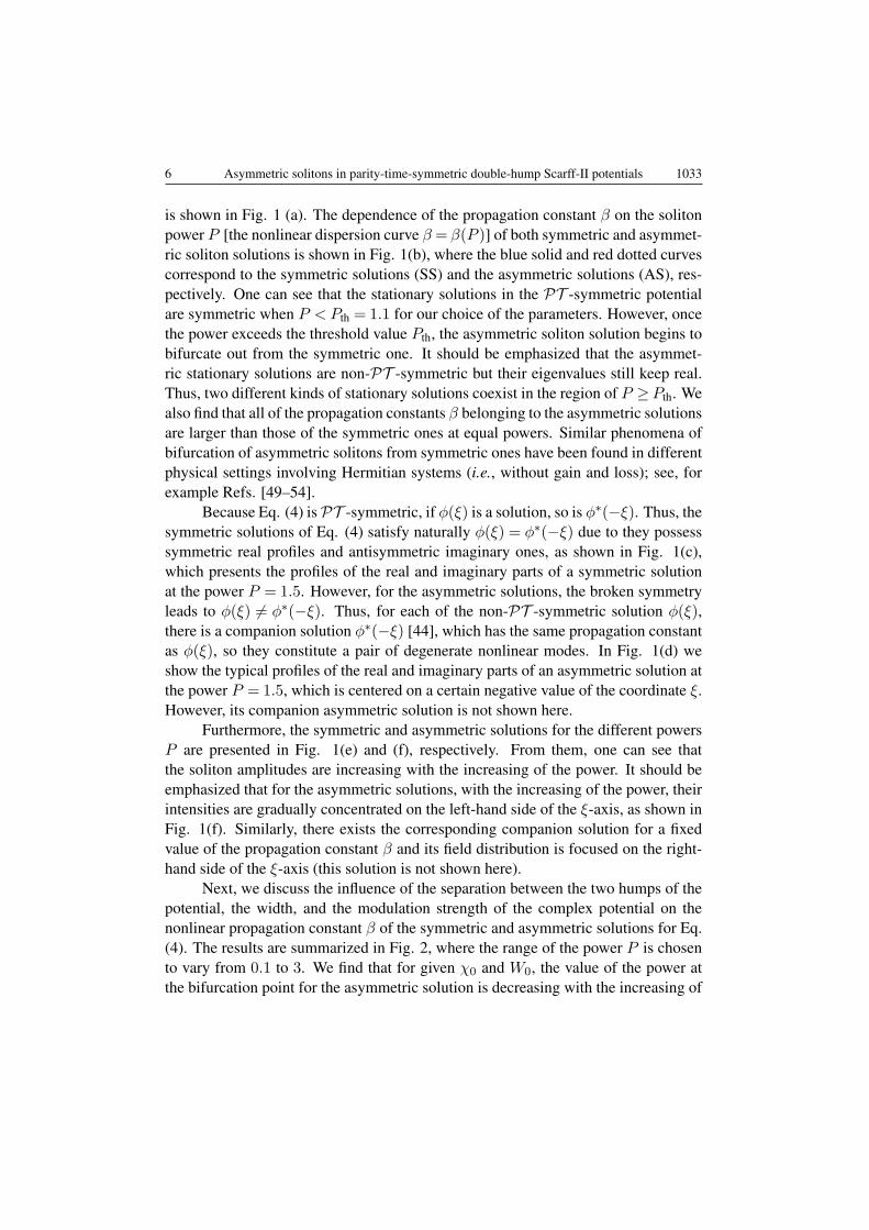
As a typical example, Fig. 3 presents the dependence of the largest real partmax(δR) of the two eigenvalues corresponding to symmetric and asymmetric solu-tions of Eq. (6) on the power P for W0 = 1, χ0 = 1, and ξ0 = 2. From it, one cansee that the symmetric solutions are stable for P < 1.1, as shown by the blue solidcurve in Fig. 3, while in the region of P ≥ 1.1, the asymmetric solutions are stable,as shown by the red dotted curve in Fig. 3. Furthermore, compared with the resultsshown in Fig. 1(b), one finds that the point of occurrence of unstable symmetric soli-ton is just the point of bifurcation of the asymmetric branch of the curve β = β(P )from the symmetric one, which is shown in Fig. 1(b).

RJP 61(Nos. 5-6), 1028–1039 (2016) (c) 2016 - v.1.3a*2016.7.20


0.5 1.0 1.5 2.0 2.5 3.0

0.0

0.2

0.4

0.6

Max(

R)

Power P

ab

c

d

Fig. 3 – (Color online) The largest real part of eigenvalues δ corresponding to symmetric (blue solidcurve) and asymmetric (red dotted curve) solutions for Eq. (6) versus the power P . Here, the parametersare W0 = 1, χ0 = 1, and ξ0 = 2.

-10 -5 0 5 10

0.0

0.4

0.8

1.2

-10 -5 0 5 10

0.0

0.4

0.8

1.2

-10 -5 0 5 10

0.0

0.4

0.8

1.2

-10 -5 0 5 10

0.0

0.4

0.8

1.2

(a1) (b

1)

(c1)

(d1)

-10 -5 0 5 100

100

200

300

400(a

2)

-10 -5 0 5 100

100

200

300

400

(b2)

-10 -5 0 5 100

100

200

300

400(c

2)

-10 -5 0 5 100

100

200

300

400(d

2)

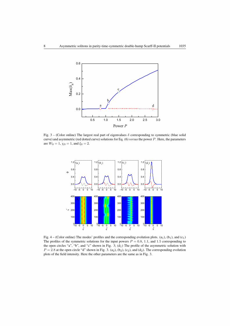
Fig. 4 – (Color online) The modes’ profiles and the corresponding evolution plots. (a1), (b1), and (c1)The profiles of the symmetric solutions for the input powers P = 0.8, 1.1, and 1.5 corresponding tothe open circles “a”, “b”, and “c” shown in Fig. 3; (d1) The profile of the asymmetric solution withP = 2.8 at the open circle “d” shown in Fig. 3. (a2), (b2), (c2), and (d2). The corresponding evolutionplots of the field intensity. Here the other parameters are the same as in Fig. 3.

RJP 61(Nos. 5-6), 1028–1039 (2016) (c) 2016 - v.1.3a*2016.7.20


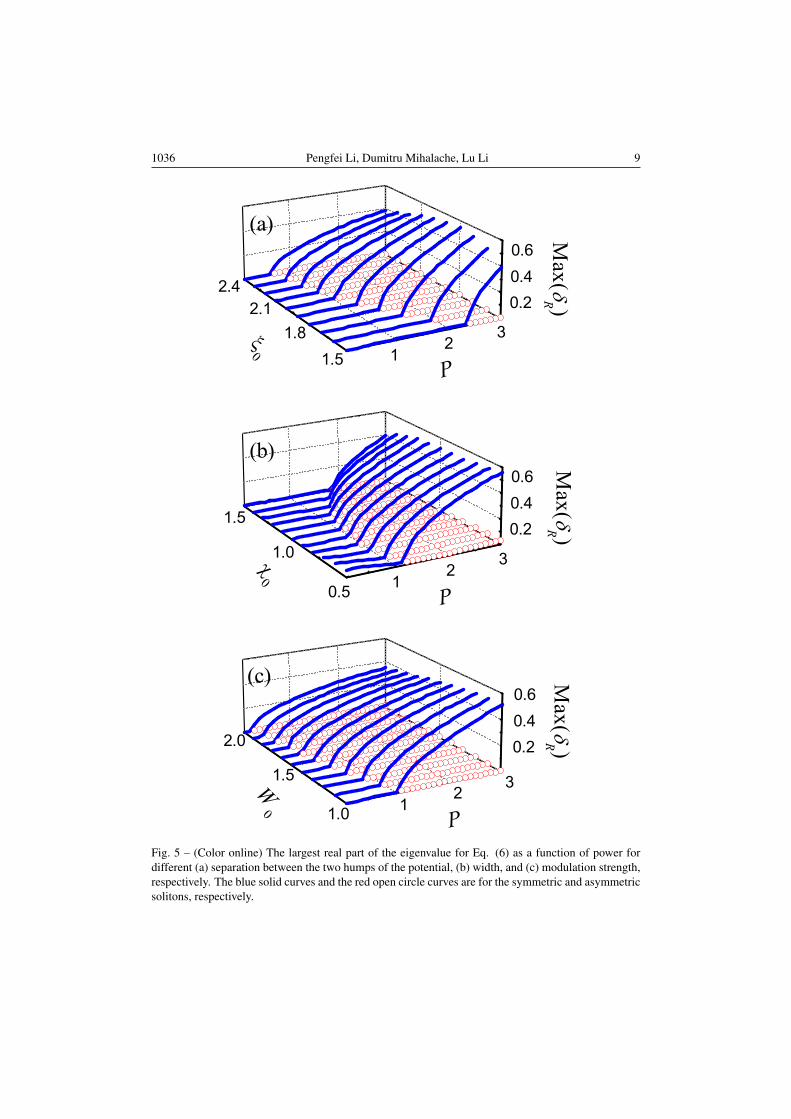
Fig. 5 – (Color online) The largest real part of the eigenvalue for Eq. (6) as a function of power fordifferent (a) separation between the two humps of the potential, (b) width, and (c) modulation strength,respectively. The blue solid curves and the red open circle curves are for the symmetric and asymmetricsolitons, respectively.

RJP 61(Nos. 5-6), 1028–1039 (2016) (c) 2016 - v.1.3a*2016.7.20


To confirm the results of linear stability analysis, we have studied the evolutionwith propagation distance ζ of four nonlinear modes by employing direct numericalsimulations of the nonlinear partial differential equation 2. The results are summa-rized in Fig. 4, in which the three symmetric modes for three choices of the inputpower P are shown in panels (a1), (b1), and (c1), whereas the asymmetric mode isshown in panel (d1). The blue solid curves show the real parts whereas the red dottedcurves display the imaginary parts of the field profiles. The largest real parts of thecorresponding eigenvalues for these solutions are marked in Fig. 3 with the opencircles “a”, “b”, “c”, and “d”, respectively.

The linear stability analysis show that the solutions at the marked points “a”and “d” should be stable, while the solutions at the points “b” and “c” should beunstable. Therefore, we perturbed the linearly stable symmetric solution shown inFig. 4(a1) and the linearly stable asymmetric solution plotted in Fig. 4(d1) by 5%random-noise perturbations. The numerical simulations clearly show that they prop-agate robustly, as displayed in Figs. 4(a2) and Figs. 4(d2). While for the linearlyunstable symmetric solutions shown in Figs. 4(b1) and 4(c1), we have performeddirect numerical simulations without adding any initial perturbations, see Figs. 4(b2) and 4(c2). Comparing Fig. 4(b2) with Fig. 4(c2), we find that the dynamicalevolutions of the unstable symmetric solutions are quite different. For the symmetricsolution with smaller nonzero real part of the eigenvalue δ, the peak values of theoptical field intensity can be switched periodically between the positions of the rightand the left humps of the potential, as shown in Fig. 4(b2). In this case, the symmetricsoliton exhibits a weak instability. However, for the solution with larger nonzero realpart of the eigenvalue δ, the peak values of the optical field intensity reside mainly onthe right side of the ξ-axis and the optical field intensity oscillate periodically withpropagation distance, as shown in Fig. 4(c2). In this case, the symmetric solitonexhibits a much stronger instability than that shown in Fig. 4(b2).

To present the influence of the separation between the two humps of the po-tential, the width, and the modulation strength of complex potential on the stabilityof either symmetric or asymmetric solitons, we investigate the dependence of thelargest real part of the eigenvalues for Eq. (6) on the input power. The results ofthese numerical simulations are summarized in Fig. 5; see the blue solid curves andthe red circle curves corresponding to symmetric and asymmetric solitons, respecti-vely. An interesting consequence of the results plotted in Fig. 5 is that the locationsof the points of bifurcations of asymmetric branches from the symmetric ones are inaccordance with the onset of unstable symmetric solitons [see a typical example ofsuch bifurcation in Fig. 1 (b)]. It indicates that instability of symmetric solutionsgives rise to a bifurcation where stable asymmetric solutions begin to appear.

RJP 61(Nos. 5-6), 1028–1039 (2016) (c) 2016 - v.1.3a*2016.7.20


5. CONCLUSIONS

In summary, we have studied in detail both the symmetric and asymmetricsoliton solutions that form in PT -symmetric double-hump Scarff-II potentials. Theresults have shown that non-PT -symmetric solitons, i.e., asymmetric solitons, bi-furcate out from the base branch of PT -symmetric solitons when the input solitonpower exceeds a certain threshold. Also, the effects of the input power, the separationbetween the two humps of the potential, the width, and the modulation strength ofthe complex-valued double-hump Scarff-II potential on the solitons’ nonlinear prop-agation constant have been investigated. The stability and the robustness to smallperturbations of these soliton solutions have been investigated and two generic insta-bility scenarios of symmetric solitons have been put forward.

Acknowledgements. This research was supported by the National Natural Science Foundationof China, through Grants No. 61475198 and 61078079, and by the Shanxi Scholarship Council ofChina, through Grant No. 2011-010. D. M. acknowledges the support from the Romanian Ministry ofEducation and Research, Project PN-II-ID-PCE-2011-3-0083.

REFERENCES

1. C. M. Bender and S. Boettcher, Phys. Rev. Lett. 80, 5243 (1998).2. C. M. Bender, D. C. Brody, and H. F. Jones, Phys. Rev. Lett. 89, 270401 (2002).3. C. M. Bender, S. Boettcher, and P. N. Meisinger, J. Math. Phys. 40, 2201 (1999).4. R. El-Ganainy, K. G. Makris, D. N. Christodoulides, and Z. H. Musslimani, Opt. Lett. 32, 2632

(2007).5. K. G. Makris, R. El-Ganainy, D. N. Christodoulides, and Z. H. Musslimani, Phys. Rev. Lett. 100,

103904 (2008).6. S. Klaiman, U. Gunther, and N. Moiseyev, Phys. Rev. Lett. 101, 080402 (2008).7. A. Guo, G. J. Salamo, D. Duchesne, R. Morandotti, M. Volatier-Ravat, V. Aimez, G. A. Siviloglou,

and D. N. Christodoulides, Phys. Rev. Lett. 103, 093902 (2009).8. C. E. Ruter, K. G. Makris, R. El-Ganainy, D. N. Christodoulides, M. Segev, and D. Kip, Nat. Phys.

6, 192 (2010);T. Kottos, ibid. 6, 166 (2010).

9. Z. H. Musslimani, K. G. Makris, R. El-Ganainy, and D. N. Christodoulides, Phys. Rev. Lett. 100,030402 (2008).

10. F. Kh. Abdullaev, Y. V. Kartashov, V. V. Konotop, and D. A. Zezyulin, Phys. Rev. A 83, 041805(R)(2011).

11. X. Zhu, H. Wang, L. Zheng, H. Li, and Y. He, Opt. Lett. 36, 2680 (2011).12. H. Li, Z. Shi, X. Jiang, and X. Zhu, Opt. Lett. 36, 3290 (2011).13. S. Hu, X. Ma, D. Lu, Z. Yang, Y. Zheng, and W. Hu, Phys. Rev. A 84, 043818 (2011).14. B. Midya and R. Roychoudhury, Phys. Rev. A 87, 045803 (2013).15. S. Nixon, L. Ge, and J. Yang, Phys. Rev. A 85, 023822 (2012).16. D. A. Zezyulin and V. V. Konotop, Phys. Rev. A 85, 043840 (2012).17. V. Achilleos, P. G. Kevrekidis, D. J. Frantzeskakis, and R. Carretero-Gonzalez, Phys. Rev. A 86,

013808 (2012).

RJP 61(Nos. 5-6), 1028–1039 (2016) (c) 2016 - v.1.3a*2016.7.20


18. M. -A. Miri et al., Phys. Rev. A 86, 033801 (2012).19. H. Xu, P. G. Kevrekidis, Q. Zhou, D. J. Frantzeskakis, V. Achilleos, and R. Carretero-Gonzalez,

Rom. J. Phys. 59, 185 (2014).20. M. Wimmer et al., Nat. Commun. 6, 7782 (2015).21. M. Wimmer, M. -A. Miri, D. N. Christodoulides, and U. Peschel, Sci. Reports 5, 17760 (2015).22. Y. He, X. Zhu, D. Mihalache, J. Liu, and Z. Chen, Phys. Rev. A 85, 013831 (2012).23. Y. He and D. Mihalache, Phys. Rev. A 87, 013812 (2013).24. D. Mihalache, Rom. Rep. Phys. 67, 1383 (2015).25. B. Liu, L. Li, and D. Mihalache, Rom. Rep. Phys. 67, 802 (2015).26. Y. Kominis, Phys. Rev. A 92, 063849 (2015).27. Z. Yan, Z. Wen, and C. Hang, Phys. Rev. E 92, 022913 (2015).28. S. V. Suchkov, B. A. Malomed, S. V. Dmitriev, and Y. S. Kivshar, Phys. Rev. E 84, 046609 (2011).29. K. Zhou, Z. Guo, J. Wang, and S. Liu, Opt. Lett. 35, 2928 (2010).30. H. Wang and J. Wang, Opt. Express 19, 4030 (2011).31. Z. Lu and Z. Zhang, Opt. Express 19, 11457 (2011).32. A. E. Miroshnichenko, B. A. Malomed, and Y. S. Kivshar, Phys. Rev. A 84, 012123 (2011).33. R. Driben and B. A. Malomed, Opt. Lett. 36, 4323 (2011).34. H. Li, X. Jiang, X. Zhu, and Z. Shi, Phys. Rev. A 86, 023840 (2012).35. Y. V. Kartashov, Opt. Lett. 38, 2600 (2013).36. C. P. Jisha, A. Alberucci, V. A. Brazhnyi, and G. Assanto, Phys. Rev. A 89, 013812 (2014).37. I. V. Barashenkov, S. V. Suchkov, A. A. Sukhorukov, S. V. Dmitriev, and Y. S. Kivshar, Phys. Rev.

A 86, 053809 (2012).38. I. V. Barashenkov, L. Baker, and N. V. Alexeeva, Phys. Rev. A 87, 033819 (2013).39. D. A. Zezyulin and V. V. Konotop, Phys. Rev. Lett. 108, 213906 (2012).40. H. Ramezani et al., Phys. Rev. A 82, 043803 (2010).41. Z. Lin et al., Phys. Rev. Lett. 106, 213901 (2011).42. Y. Lumer, Y. Plotnik, M. C. Rechtsman, and M. Segev, Phys. Rev. Lett. 111, 263901 (2013).43. R. Li, P. Li, and L. Li, Proc. Romanian Acad. A 14, 121 (2013).44. J. Yang, Opt. Lett. 39, 5547 (2014).45. J. Yang, Stud. Appl. Math. 132, 332 (2014).46. J. Yang, Phys. Rev. E 91, 023201 (2015).47. H. Chen and S. Hu, Phys. Lett. A 380, 162 (2016).48. Z. Ahmed, Phys. Lett. A 282, 343 (2001).49. N. N. Akhmediev and A. Ankiewicz, Phys. Rev. Lett. 70, 2395 (1993).50. B. A. Malomed, I. M. Skinner, P. L. Chu, and G. D. Peng, Phys. Rev. E 53, 4084 (1996).51. P. G. Kevrekidis, Z. Chen, B. A. Malomed, D. J. Frantzeskakis, and M. I. Weinstein, Phys. Lett. A

340, 275 (2005).52. M. Matuszewski, B. A. Malomed, and M. Trippenbach, Phys. Rev. A 75, 063621 (2007).53. B. A. Malomed, Nat. Photon. 9, 287 (2015).54. J. F. Jia, Y. P. Zhang, W. D. Li, and L. Li, Opt. Commun. 283, 132 (2010).55. Jianke Yang, Nonlinear waves in integrable and nonintegrable systems, Society for Industrial and

Applied Mathematics, Philadelphia, 2010.

RJP 61(Nos. 5-6), 1028–1039 (2016) (c) 2016 - v.1.3a*2016.7.20

asymmetric solitons in parity-time-symmetric double-hump ... · 2 asymmetric solitons in...

Documents