asymmetric incentives in subsidies - koichiro ito

Introduction Data Identification Strategy Results Conclusion

Asymmetric Incentives in Subsidies:Evidence from a Large-Scale Electricity Rebate Program

Koichiro Ito, Boston University

[email protected]

October, 2014

1 / 37


Residential Electricity Sector - The Lowest Abatement Cost?

2 / 37


Economists are usually skeptical about this optimistic view

Price elasticity of residential electricity demand is small

A significant price increase is often politically infeasible

What can we do?

3 / 37


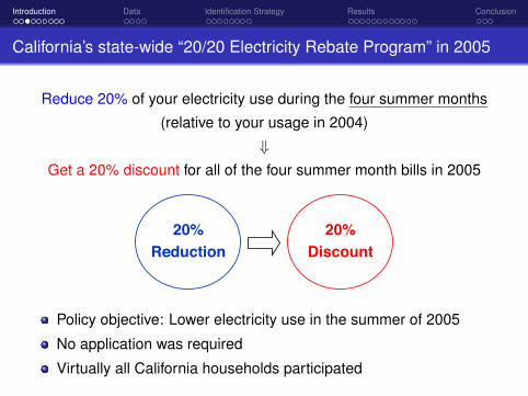
California’s state-wide “20/20 Electricity Rebate Program” in 2005

Reduce 20% of your electricity use during the four summer months

(relative to your usage in 2004)

⇓Get a 20% discount for all of the four summer month bills in 2005

20% !Reduction!

20% !Discount!

Policy objective: Lower electricity use in the summer of 2005

No application was required

Virtually all California households participated4 / 37


I examine whether the program achieved its policy goal

Policy goal:

Encourage households to reduce summer electricity consumption

Research questions:

1 How much electricity was saved because of the program?

2 What was the program’s cost-effectiveness?

Why do we care about the questions?

5 / 37


Reason (1) A large scale program with a significant expense

The summer four billing months in 2005

Utility Revenue Rebated Rebate

($M) Households ($M)

PG&E 1,322 8.24% 10.79

SCE 1,257 7.91% 10.61

SDG&E 363 9.07% 4.33

The rebate expense was close to 1% of each utility’s revenue

The expense was eventually paid by ratepayers

6 / 37


Reason (2) Similar programs are widely used to promote

conservation

Similar Rebate Programs in California:

Summer electricity 20/20 rebate program in 2001 and 2002 (Reiss

and White 2008)

Winter gas rebate program in every year in PG&E

Peak-Time Rebate Program:

Anaheim (Wolak 2006)

Washington DC (Wolak 2011)

Many other electric utilities in the US and other countries

7 / 37


Reason (3) However, the cost-effectiveness has been

controversial

Critique:

Many households may get rebates without conservation efforts

Example 1: If they get milder weather in the target year

Example 2: If they had a visitor in the base year

Evidence from years that did not have a rebate program:

Year Weather %Households with

20% or more reduction

2003 to 2004 Cooler in 2004 14.3%

1999 to 2000 Warmer in 2000 6.8%

8 / 37


How to identify the causal effect of the program?

Household electricity consumption can be affected by:

1 Weather

2 Macro economic shocks

3 Electricity prices

4 The treatment effect of the program

5 Other conservation campaigns

The key question is how to disentangle (4) from others

9 / 37


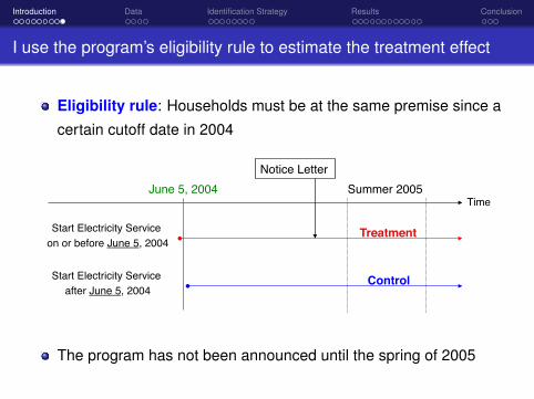
I use the program’s eligibility rule to estimate the treatment effect

Eligibility rule: Households must be at the same premise since a

certain cutoff date in 2004

Treatment!

Time!Summer 2005!June 5, 2004!

Control!

Start Electricity Service! on or before June 5, 2004!

Notice Letter!

Start Electricity Service! after June 5, 2004!

The program has not been announced until the spring of 2005

10 / 37


Road Map

1 Introduction

2 Data

3 Identification Strategy

4 Result

5 Conclusion

11 / 37


Data: Household-level Monthly Billing Records

Household-level monthly billing records

1 PG&E (Pacific Gas & Electric)2 SCE (Southern California Edison)3 SDG&E (San Diego Gas & Electric)

Each monthly record includes:

1 Account ID2 Nine-digit ZIP code (e.g. 94720-5180)3 Climate zone defined by the utilities4 Tariff schedules5 Billing period (e.g. May15-Jun14)6 Electricity consumption (kWh) during the billing period7 Account start date and close date

12 / 37

Sierra Pacific Power

PacifiCorp

PG&E

Mountain Utilities

Bear ValleyElectric

SDG&E

SCEPG&E


PacifiCorp

PG&E

Mountain Utilities

Bear ValleyElectric

SDG&E

SCEPG&E

California's Electric Investor-Owned Utilities (IOUs)


Data: Weather and Demographic Data

Weather data from the Cooperative Station Dataset by NOAA

Daily data at the weather station levelDaily max and min temperature

Demographic data from the US Census in 2000

At the Census Block Group (CBG) levelMedian household income

14 / 37


Identification Strategy

1 Introduction

2 Data

3 Identification Strategy

4 Result

5 Conclusion

15 / 37


I compare electricity consumption between treatment and

control groups

Treatment!

Time!Summer 2005!June 5, 2004!

Control!

Start Electricity Service! on or before June 5, 2004!

Notice Letter!

Start Electricity Service! after June 5, 2004!

1 Essentially random assignment of the treatment across the cutoff

2 No strategic entering b/c the program cannot be anticipated in 2005

3 No self-selection b/c all eligible households automatically enrolled

16 / 37



control groups

Account open date !

Change in Consumption !from 2004 to 2005!

Cutoff date !(eg. June 5, 2004 for SCE) ! 17 / 37



control groups

Account open date !


Cutoff date !(eg. June 5, 2004 for SCE) !

Treatment Group! Control Group!

18 / 37



control groups

Account open date !




19 / 37



control groups

Account open date !




Treatment Effect !

20 / 37


Estimation: A Regression Discontinuity Design with a

sharp discontinuity

∆ln(yi ,t) = α · Treati(xi) + f (xi) + θzip,t + δcycle + εi ,t

yi,t = household i ’s electricity consumption in billing period t

∆ln(yi,t) = differences in log between the same month of 2005 and 2004

xi = service start date

Treati = 1 if xi ≤ c, where c = the cutoff date to be eligible

To control for f (xi)

Limit observations in narrow windows from the cutoff dateUse flexible parametric function for f (xi) orLocal liner regressions (Imbens and Lemieux 2008)

21 / 37


Parametric and Nonparametric Controls

Method 1: Include a flexible parametric function of Xi:

4lnyit = α+ β · Treati +S∑

s=1

(γs ·Xsi + θs · Treati ·Xs

i ) + δzip + δcycle + εi,t

Method 2: Non-parametrically control for Xi by the local linear

regression using a triangular kernel (Imbens and Lemieux 2008)

4lnyit = K

(Xi − ch

)·(α+ β · Treati + γ ·Xi + θ · Treati ·Xi + δzip + δcycle + εi,t)

22 / 37


Estimation Results for Southern California Edison (SCE)


PacifiCorp

PG&E

Mountain Utilities

Bear ValleyElectric

SDG&E

SCEPG&E


PacifiCorp

PG&E

Mountain Utilities

Bear ValleyElectric

SDG&E

SCEPG&E

California's Electric Investor-Owned Utilities (IOUs)

23 / 37

Figure 2: Testing the Validity of the Regression Discontinuity Design

500

1000

1500

2000

−100 −50 0 50 100Account Open Date Relative to Cutoff Date

1) Number of new accounts opened per day

1967

1968

1969

1970

1971


2) Median year structure built

48000

49000

50000

51000

52000


3) Median customer income ($)

840

850

860

870

880


4) Median rent ($)

Note: The horizontal axis shows the account open date relative to the cuto↵ date of the programeligibility, which was June 5, 2004. Each dot shows the local mean with a 15-day bandwidth. Thesolid line shows the local linear fit and the dashed lines present the 95 percent confidence intervals.The confidence intervals for the fitted lines for variables from Census data are adjusted for clusteringat the census block group level.

36


SCE Climate Zone 16: Representative Cities (Bakersfield)

Dependent variable:

ln(yi,Sep2005 )− ln(yi,Sep2004 )

Dot: Local average usingfifteen days windows

Solid line: Local linearregression

Dashed line: Parametricregression

Zip code dummy and billingcycle dummy are included

−.1

−.0

50

.05

.1


Point estimate (robust standard error):

-.101** (.032)

25 / 37


SCE Climate Zone 15: Representative Cities (Palm Dessert, Death Valley)

Dependent variable:






−.1

−.0

50

.05

.1



-.091*** (.040)

26 / 37


SCE Climate Zone 10:Representative Cities (Santa Barbara, Long Beach and Irvine)

Dependent variable:






−.1

−.0

50

.05

.1



.005 (.007)

27 / 37

Figure 4: The Di↵erence in Log Consumption between Treatment and ControlGroups

Panel A. Coastal Climate Zones

−.1

−.05

0

.05

1 2 3 4 5 6 7 8 9 10Billing Month in 2005

RD Estimates 95% Confidence Intervals

Panel B. Inland Climate Zones

−.1

−.05

0

.05

1 2 3 4 5 6 7 8 9 10Billing Month in 2005

RD Estimates 95% Confidence Intervals

Note: This figure presents the RD estimates of the di↵erence in log consumption between the treat-ment and control groups. Customer fixed e↵ects are subtracted by using consumption data beforeJanuary 2005. I use a 90-day bandwidth and quadratic controls for the trend of the running variable,which is the same specification used to obtain my main estimation results shown in Table 2.

38

Table 2: RD Estimates of the E↵ect of Rebate Incentives on Energy Conservation

(1) (2) (3) (4)

Treatment Effect -0.001 -0.042(0.002) (0.013)

Treatment Effect 0.003 -0.034in May (0.003) (0.015)

Treatment Effect -0.001 -0.055in June (0.003) (0.017)

Treatment Effect 0.004 -0.041in July (0.004) (0.019)

Treatment Effect -0.003 -0.037in August (0.004) (0.018)

Treatment Effect -0.004 -0.056in Septermber (0.003) (0.016)

Observations 2,540,472 2,540,472 208,537 208,537

Coastal Climate Zones Inland Climate Zones

Note: This table shows the RD estimates of the e↵ect of rebate incentives on energy conservation.The dependent variable is the log of electricity consumption. I estimate equation (2) with a 90-day bandwidth and quadratic functions to controls for the running variable. The standard errors areclustered at the customer level to adjust for serial correlation.

40

Table 3: Robustness Checks: Alternative Bandwidths and Specifications

(1) (2) (3) (4) (5) (6)

Treatment Effect 0.004 0.003 0.005 -0.034 -0.039 -0.029in May (0.004) (0.003) (0.004) (0.015) (0.014) (0.017)

Treatment Effect -0.002 -0.001 -0.003 -0.055 -0.059 -0.05in June (0.004) (0.004) (0.004) (0.017) (0.016) (0.019)

Treatment Effect 0.004 0.005 0.005 -0.041 -0.039 -0.042in July (0.004) (0.004) (0.005) (0.019) (0.017) (0.022)

Treatment Effect -0.004 -0.005 -0.003 -0.036 -0.034 -0.035in August (0.004) (0.004) (0.004) (0.018) (0.016) (0.020)

Treatment Effect -0.005 -0.003 -0.004 -0.056 -0.053 -0.052in Septermber (0.003) (0.004) (0.004) (0.016) (0.015) (0.018)

Controls for f(x) Local linear Quadratic Quradratic Local linear Quadratic Quradratic Bandwidth 90 days 120 days 60 days 90 days 120 days 60 daysObservations 2,540,472 3,325,388 1,707,589 208,537 237,264 162,067

Coastal Climate Zones Inland Climate Zones

Note: This table shows RD estimates with di↵erent bandwidth choices and alternative controls forthe running variable. The dependent variable is the log of electricity consumption. The standarderrors are clustered at the customer level to adjust for serial correlation.

41

Table 6: Potential Long-run E↵ects

2005 2006 2007 2008 2005 2006 2007 2008

Treatment Effect -0.001 0.001 -0.002 0.002 -0.042 -0.040 -0.048 -0.043(0.002) (0.003) (0.004) (0.004) (0.013) (0.018) (0.021) (0.022)

Coastal Inland

Note: This table shows the RD estimates of the potential long run e↵ect of rebate incentives onenergy conservation. The dependent variable is the log of electricity consumption. The treatmentvariable is the interaction of the treatment group and the summer of 2006, 2007, and 2008, which areone, two, and three years after the rebate program. The standard errors are clustered at the customerlevel to adjust for serial correlation.

43


What Drives Heterogeneous Treatment Effects?

At least two possible reasons:

1 Climate conditions (air conditioner usage)

2 Income levels

32 / 37

Table 4: RD Estimates Interacted with Income, Climate, and Air Conditioner Satu-ration

(1) (2) (3) (4)

Treatment 0.095 -0.297 -0.199 -0.478(0.051) (0.055) (0.077) (0.056)

Treatment*Ave.Temp.(F) -0.0015 -0.0016(0.0007) (0.0008)

Treatment*ln(Income) 0.029 0.031 0.044(0.005) (0.005) (0.003)

Treatment*Air Conditionar -0.014(0.005)

Observations 2,749,009 2,749,009 2,749,009 2,749,009

Note: This table presents the RD estimates of the e↵ect of rebate incentives on energy conservationinteracted with income, climate conditions, and air conditioner saturation. The dependent variableis the log of electricity consumption. I use a 90-day bandwidth and quadratic controls for the trendin the running variable. Income is at the census block group level. Average temperature and airconditioner saturation (the ratio of customers who own air conditioners) are at the five-digit zip codelevel. The standard errors are clustered at the customer level to adjust for serial correlation.

Table 5: Quantile Regressions on the Change in Log Consumption for Inland Cli-mate Zones

p5 p10 p25 p50 p75 p90 p95

Treatment 0.034 -0.099 -0.078 -0.007 -0.020 -0.019 -0.025(0.056) (0.035) (0.018) (0.018) (0.019) (0.033) (0.063)

Observations 37,914 37,914 37,914 37,914 37,914 37,914 37,914

Note: This table presents the quantile RD estimates of the e↵ect of rebate incentives on energyconservation. The dependent variable is the change in the log of electricity consumption from 2004to 2005. I use a 90-day bandwidth and quadratic controls for the trend in the running variable. Thestandard errors are clustered at the customer level to adjust for serial correlation.

42

Table 8: Program Cost Per Estimated Reductions in Consumption and CarbonDioxide

Coastal Inland Total

Number of Customers 3,190,027 299,178 3,489,205

Consumption in Summer 2005 (kWh) 8,247,457,920 1,154,292,248 9,401,750,168

Direct Program Cost for Rebate ($) 9,358,919 1,250,621 10,609,540

Estimated Reduction (kWh) 9,908,840 50,605,714 60,514,555

Estimated Reduction in Carbon Dioxide (ton) 4,459 22,773 27,232

Program Cost Per kWh ($/kWh) 0.945 0.025 0.175

Program Cost Per Carbon Dioxide ($/ton) 2,099 55 390

Program Cost Per Carbon Dioxide ($/ton) 2,090 46 381(Adjusted for non-carbon external benefits)

Note: This table reports the cost-benefit analysis of the 20/20 program for SCE’s coastal areas,inland areas, and all service areas. Row 1 shows the number of residential customers who maintainedtheir accounts in the summer of 2004 and 2005. Row 2 presents the aggregate consumption in thesummer months. Row 3 reports the aggregate amount of rebate paid to customers. Row 4 shows theestimated kWh reduction from the treatment e↵ect of the program. Row 5 translates this reductioninto the reduction in carbon emissions by using the average carbon intensity of electricity consumedin California, which is 0.9 lb. per kWh according to California Air Resources Board (2011).

45


Summary

This paper uses a RDD to estimate the effect of the state-wideconservation rebate program in California

5 to 10% of consumption reductions in inland areas

Virtually no effect in most of the coastal areas

Higher temperature areas→ Larger treatment effects

Lower income areas→ Larger treatment effects

Cost-effectiveness:

Inland areas: 2.5 cents per kWh reduction

Coastal areas: 94.5 cents per kWh reduction

35 / 37


Policy Implications

Under the current rebating scheme, many households receive

rebates for reasons unrelated to their conservation efforts

The cost-effectiveness would be very poor if the treatment effect is

not sufficiently large (e.g. the findings for the coastal areas)

Focusing on households with lower income and warmer climate

areas may improve the cost-effectiveness

36 / 37


Thank you

Thank you for your attention!

37 / 37

asymmetric incentives in subsidies - koichiro ito

Documents