astronomy c eso 2007 astrophysics - open research …oro.open.ac.uk/24864/1/glenn.pdf2 centre for...
TRANSCRIPT

A&A 477, 557–571 (2008)DOI: 10.1051/0004-6361:20078104c© ESO 2007
Astronomy&
Astrophysics
A SCUBA survey of bright-rimmed clouds
L. K. Morgan1 ,, M. A. Thompson2, J. S. Urquhart3, and G. J. White1,4,5
1 CAPS, The University of Kent, Canterbury, Kent CT2 7NR, UKe-mail: [email protected]
2 Centre for Astrophysics Research, Science and Technology Research Institute, University of Hertfordshire, College Lane,Hatfield AL10 9AB, UK
3 School of Physics and Astronomy, University of Leeds, Leeds LS2 9JT, UK4 Space Physics Division, Room 1.71, Space Science & Technology Division, CCLRC Rutherford Appleton Laboratory, Chilton,
Didcot, Oxfordshire OX11 0QX, UK5 Dept. of Physics & Astronomy, The Open University, Walton Hall, Milton Keynes MK7 6AA, UK
Received 17 June 2007 / Accepted 29 October 2007
ABSTRACT
Context. Bright-rimmed clouds (BRCs) are potential examples of triggered star formation regions, in which photoionisation drivenshocks caused by the expansion of HII regions induce protostellar collapse within the clouds.Aims. The main purpose of the paper is to establish the level of star formation occuring within a known set of BRCs. A secondaryaim is to determine the extent, if any, to which this star formation has been promulgated by the process of photoionisation triggering.Methods. A primary set of observations is presented obtained with submillimeter SCUBA observations and archival data from near-IR and mid- to far-IR have been explored for relevant observations and incorporated where appropriate.Results. SCUBA observations show a total of 42 dense cores within the heads of 44 observed BRCs drawn from a catalogue ofIRAS sources embedded within HII regions, supportive of the scenario proposed by RDI models. The physical properties of thesecores indicate star formation across the majority of our sample. This star formation appears to be predominately in the regime ofintermediate to high mass and may indicate the formation of clusters. IR observations indicate the association of early star formingsources with our sample. A fundamental difference appears to exist between different morphological types of BRC, which mayindicate a different evolutionary pathway toward star formation in the different types of BRC.Conclusions. Bright-rimmed clouds are found to harbour star formation in its early stages. Different evolutionary scenarios are foundto exist for different morphological types of BRC. The morphology of a BRC is described as type “A”, moderately curved rims, type“B”, tightly curved rims, and “C”, cometary rims. “B” and “C” morphological types show a clear link between their associated starformation and the strength of the ionisation field within which they are embedded.An analysis of the mass function of potentially induced star-forming regions indicate that radiatively-driven implosion of molecularclouds may contribute significantly toward the intermediate to high-mass stellar mass function.
Key words. stars: formation – ISM: HII regions – submillimetre
1. Introduction
Bright-rimmed clouds (BRCs) are small molecular clouds foundat the edges of large HII regions. These clouds are potentialexamples of triggered star-forming regions, whereby shocksdriven into the BRC by the photoionisation of the cloud exte-rior results in the collapse (and perhaps even the formation) ofsub-critical molecular cores within the cloud (e.g. Deharvenget al. 2005; Elmegreen 1998; Sugitani et al. 1991). The pro-cess of photoionisation-induced collapse is usually known asradiative-driven implosion or RDI (Bertoldi 1989; Lefloch &Lazareff 1995, 1994). The RDI of molecular cores at the pe-riphery of HII regions may thus be responsible for subsequentgeneration of star formation, amounting to a possible cumula-tive total of several hundred new stars per HII region (Oguraet al. 2002) and perhaps 15% or more of the low-to-intermediatemass stellar mass function (Sugitani et al. 1991). IRAS-selectedprotostars associated with HII regions are systematically more
Appendix is only available in electronic form athttp://www.aanda.org Present address: NRAO, Green Bank Telescope, PO Box 2, GreenBank, WV 24944, USA.
luminous than those that are not (Dobashi et al. 2001). This high-lights a trend toward higher mass star formation and greater starformation efficiency. Confirming bright-rimmed clouds as star-forming and quantifying the nature and location of their star for-mation thus provides important insights into the clustered modeof star formation and the overall star formation efficiencies ofmolecular clouds.
Sugitani et al. (1991), hereafter referred to as SFO91,searched the Sharpless HII region catalogue (Sharpless 1959)for bright-rimmed clouds associated with IRAS point sources,their selection was based upon the FIR colours thought to iden-tify YSOs/protostars. Later, Sugitani & Ogura (1994) – SO94– extended their search to include bright-rimmed clouds fromthe ESO(R) Southern Hemisphere Atlas. A total of 89 opticallyidentified bright-rimmed clouds have been found to be associ-ated with IRAS point sources. For brevity (and consistency withSIMBAD), we will refer to the combined SFO91 and SO94 cat-alogues as the SFO catalogue. Whilst a few individual cloudsfrom the SFO catalogue have been studied in detail (e.g. Leflochet al. 1997; Megeath & Wilson 1997; Codella et al. 2001;Thompson et al. 2004b; Thompson & White 2004; Urquhartet al. 2004, 2006, 2007) and shown to harbour protostellar cores,
Article published by EDP Sciences and available at http://www.aanda.org or http://dx.doi.org/10.1051/0004-6361:20078104

558 L. K. Morgan et al.: A SCUBA survey of bright-rimmed clouds
the question of whether star formation is a common occurencewithin BRCs (irrespective of the formation mechanism) is stillunresolved.
We are in the process of carrying out a star formation censusof SFO bright-rimmed clouds in order to determine the currentlevel of star formation within these sources and to relate it totheir physical properties and morphologies with respect to theirionising star(s). In two previous publications we reported obser-vations of the ionised gas surrounding the bright-rimmed clouds(Thompson et al. 2004a; Morgan et al. 2004). Here we report aSubmillimetre Common User Array (SCUBA) imaging surveyof the submillimetre continuum emission from the clouds, in or-der to reveal the presence of compact, potentially star-forming,dust cores within the clouds and to contrast the properties ofthese cores with those found in other star-forming regions. Weuse NIR archival data from the 2 mm all-sky survey (2MASS)database to construct colour-colour diagrams to investigate thecurrent level of star formation within these clouds and to iden-tify YSOs. We examine the kinematics and temperature of thedust cores revealed by our SCUBA observations to show thata number of the SFO bright-rimmed clouds are associated withactive star formation.
2. Observations
2.1. SCUBA continuum maps
Simultaneous 450 and 850 µm images were obtained usingSCUBA (Holland et al. 1999) on the James Clerk Maxwell tele-scope (JCMT1). SCUBA is a dual-camera system comprised oftwo bolometer arrays which simultaneously sample a similarfield of view (∼2′ square). Each bolometer array is arranged in ahexagonal pattern and both arrays are observed using a dichroicbeamsplitter. The 91 pixel short-wave array is optimised for op-eration at 450 µm and the 37 pixel long-wave array of 37 pixelsis optimised for operation at 850 µm. The arrays do not fullyspatially sample the field-of-view and in order to provide fully-sampled images the secondary mirror of the JCMT is moved in a64-point pattern (“jiggling”) whilst also chopping at a frequencyof 1 Hz to remove sky emission. This procedure is commonlyknown as a “jiggle-map”.
Our initial source list was formed from those BRCs in theSFO catalogue lying within the declination limits visible fromthe JCMT, which gives a total number of 50 clouds (45from the mainly northern hemisphere SFO91 catalogue and 5from the southern hemisphere SO94 catalogue). We also in-cluded the two bright-rimmed clouds SFO 11NE and SFO 11E inour sample. These two clouds lie in close proximity to the bright-rimmed cloud SFO 11 (Ogura et al. 2002). SCUBA observationsof these three clouds have already been reported in Thompsonet al. (2004b). Thus our initial source list comprised 52 bright-rimmed clouds. However, observations of only 47 clouds werecompleted, due to the fact that our observations were performedin the flexibly-scheduled mode used at the JCMT. As observa-tions of three of these clouds have been previously reported byThompson et al. (2004b) we present here observations of theremaining 44 clouds. Flexibly scheduled observations are notscheduled over a pre-defined period but are carried out accordingto the appropriate weather (atmospheric opacity) band, the visi-bility of the sources from the telescope and the scientific priority
1 The JCMT is operated by the Joint Astronomy Centre on behalfof PPARC for the United Kingdom, the Netherlands Organisation ofScientific Research and the National Research Council of Canada.
of the observations. The observations of the BRCs in our sampletook place over several days from November 2001 to April 2002.
As the angular diameters of most of the clouds in the SFOcatalogue are comparable to the field-of-view (FOV) of SCUBAwe obtained single jiggle-maps for each cloud. A small num-ber of clouds in the sample either have larger angular diametersor lie in associations that are larger than the SCUBA FOV. Inthese cases multiple overlapping jiggle-maps were obtained andmosaiced together to cover the cloud or association. Varying in-tegration times were used for each cloud, depending upon the at-mospheric opacity and the brightness of the submillimetre emis-sion that was detected. A chop throw of 120′′ was initially usedfor each jiggle-map but after inspection of the first images thiswas changed to 180′′ to avoid chopping onto extended emission.The atmospheric opacity was measured using the CSO 225 GHzradiometer and by performing hourly skydips with SCUBA atthe approximate azimuth of each observation. Typical sky opac-ities were 2.270 at 450 µm and 0.326 at 850 µm.
The data were reduced and calibrated in the standard man-ner using the SCUBA User Reduction Facility (SURF) (Jenness& Lightfoot 2000) and the Starlink image analysis packageKAPPA (Currie & Berry 2002). Absolute flux calibration wasperformed using calibration maps of the primary calibrators,Uranus and Mars, or the secondary calibrators CRL 618,CRL 12688, 16293-2422, IRC 10216 and OH 231.8 depend-ing upon the observation date, time and sky position. Predictedfluxes for Uranus and Mars were estimated using the valuesgiven by the Starlink package FLUXES (Privett et al. 1998) andpredicted fluxes for the secondary calibrators were taken fromthe JCMT calibrator webpage2.
The JCMT has a well known error beam contribution thatmay be modelled by a combination of two circularly symmetricgaussian functions representing the main and error beams. Weremoved the error-beam contribution to the flux by deconvolvingthe calibrated images with a model two-component beam deter-mined from azimuthally averaged maps of the primary calibra-tors (using the method outlined in Hogerheijde & Sandell 2000;Thompson et al. 2004b). It is well known that CLEAN processesdo poorly with extended structure and therefore as many of oursources are extended on the scale of the JCMT primary beamCLEANing was performed only until negative components wereencountered. Images were then restored to a resolution of 14′′.This is the native resolution at 850 µm and hence smooths the450 µm data from its native resolution of 8′′. The smoothinghas the advantages of facilitating the comparison of the 450 µmand 850 µm images and improving the signal-to-noise ratio ofthe 450 µm data to extended emission by approximately a factorof 3.
2.2. Archival data
2.2.1. IRAS HiRes data
IRAS HiRes images at 12, 25, 60 and 100 µm were obtainedfrom the NASA/IPAC Infrared Science Archive3 to comple-ment the SCUBA data, extend the FIR wavelength coverageof each source and enable the spectral energy distribution(SED) to be measured. The IRAS HiRes image constructionalgorithm utilises the maximum correlation method (MCM)
2 http://www.jach.hawaii.edu/JACpublic/JCMT/Continuum_observing/SCUBA/astronomy/calibration
3 http://irsa.ipac.caltech.edu

L. K. Morgan et al.: A SCUBA survey of bright-rimmed clouds 559
(Aumann et al. 1990) in the enhancement of the original all-skysurvey data. The angular resolution and signal-to-noise ratio ofHiRes data varies depending upon the number of deconvolutioniterations used and the position within the image. HiRes imagesare also subject to a number of processing artefacts, most notableof which are the negative “bowls” surrounding bright sourcesthat are known as ringing. This effect is much more prevalent athigher wavelengths, we found that 60 and 100 µm images mayneed significant correction, while 12 and 25 µm images neededvery little. Corrections to source fluxes were estimated throughmeasuring any negative offset present close to the source andadjusting the source flux accordingly.
For IRAS data sets with typical coverages, correction factorvariance (CFV) values reach 0.01–0.001 at strong, convergedsources (Levine & Surace 1993). It was found that the defaultprocessing parameters for HiRes images were not sufficient toachieve this in the majority of our images. Visual inspection ofthe produced maps allowed us to discount the possibility that theregions were saturated, overly noisy or contained “bad” scans.Coverage maps of all of our sources allowed us to ascertain thelevel of coverage per source, as well as the uniformity of thecoverage over the beam area. This was good for all sources andso we iterated all sources until we reached the recommendedCFV values of 0.01–0.001, this was generally found to be af-ter ∼150–200 iterations, similar to the number of iterations usedin the analysis of the Serpens star-forming cloud core (Hurt &Barsony 1996)
Typical (mean) angular resolutions were 36′′, 34′′, 49′′ and73′′ at 12, 25, 60 and 100 µm respectively, which are generallyonly sufficient to identify the strongest cores in each SCUBAfield as point sources. The absolute calibration uncertainties ofthe HiRes data are estimated to be around 20%, which is similarto the original IRAS survey data.
Individual fluxes for each of the SCUBA cores were mea-sured from the HiRes images by aperture photometry and arelisted in Table 1. It should be noted that the fluxes tabulated herediffer from those given for each source in the IRAS point sourcecatalogue. This is, no doubt, due to the nearly five-fold enhancedresolution of the HiRes images over the original IRAS survey.HiRes fluxes are typically 2–3 times lower than those listed inthe IRAS PSC with the largest differences seen in the 12 and25 µm bands. A comparison of the luminosities as determinedfrom HiRes fluxes to those derived by SFO91 will be addressedin Sect. 4.3. This is likely to have a large effect upon the conclu-sions of SFO91 who concluded that the IRAS sources embeddedwithin these bright-rims had large luminosities in comparison toIRAS sources embedded within dark globules and other densecores. With our improved IR resolution and extended coverageof the sources SEDs we aim to investigate the true luminosityfunction of the Sugitani catalogue.
2.2.2. 2MASS
Data from the near-infrared J, H and Ks 2MASS catalogue(Cutri et al. 2003) were obtained to search for protostars and em-bedded young stellar objects (YSOs) associated with the BRCs.The catalogue data were obtained from the 2MASS Point Sourcecatalogue held at the NASA/IPAC Infrared Science Archive4.The accuracy of the photometric measurements in the 2MASSPoint Source Catalogue is between 1 and 2%, though can bemuch larger for weak sources. The limiting magnitudes at J, H
4 http://irsa.ipac.caltech.edu
Table 1. Fluxes of each source as measured in IRAS HiRes images.
Source IRAS HiRes flux(Jy)12 µm 25 µm 60 µm 100 µm
SFO 01 1.3 2.9 46.8 173.2SFO 02 0.9 1.5 13.6 51.9SFO 03 0.2 1.5 12.2 52.1SFO 04 0.5 0.9 11.9 25.2SFO 05 1.8 30.2 95.0 155.4SFO 06 0.2 0.3 3.4 15.5SFO 07 0.5 1.1 18.0 74.9SFO 09 0.4 0.6 15.5 47.6SFO 10 1.0 1.9 25.6 72.8SFO 12 0.4 1.1 16.7 36.6SFO 13 1.2 2.3 35.9 84.5SFO 14 5.2 49.6 420.2 534.7SFO 15 0.2 1.0 7.3 23.6SFO 16 0.1 1.3 14.6 23.0SFO 17 0.1 0.7 3.3 16.0SFO 18 0.1 1.0 14.0 22.2SFO 23 0.1 0.4 4.1 9.4SFO 24 0.3 0.6 8.7 26.0SFO 25 0.3 1.4 17.9 44.1SFO 26 0.2 0.3 4.7 17.7SFO 27 0.5 1.8 15.8 97.2SFO 28 1.4 1.6 37.4 126.6SFO 29 0.3 0.3 5.7 29.5SFO 30 9.1 69.0 665.0 901.2SFO 31 1.0 3.8 26.2 127.5SFO 32 0.4 0.2 6.8 25.7SFO 33 0.2 0.8 7.0 43.4SFO 34 0.6 1.0 6.8 24.7SFO 35 0.3 0.6 4.2 22.7SFO 36 0.3 1.7 14.9 54.8SFO 37 1.8 11.2 35.6 45.2SFO 38 0.9 3.6 62.2 172.2SFO 39 0.7 3.8 17.4 33.7SFO 40 0.5 0.4 5.6 25.8SFO 41 0.5 0.7 5.7 21.6SFO 42 0.3 0.6 5.6 20.1SFO 43 2.8 12.1 95.4 144.0SFO 44 0.6 8.7 124.4 300.2SFO 45 0.1 0.3 1.2 7.7SFO 77 0.5 5.1 55.7 67.1SFO 78 0.4 1.1 9.7 37.2SFO 87 3.3 4.2 138.5 430.6SFO 88 1.6 3.8 120.7 396.4SFO 89 3.8 5.5 111.9 330.2
and Ks in the 2MASS catalogue are 15.8, 15.1 and 14.3 respec-tively.
3. Results and analysis
Of the forty-four BRCs that were observed, 39 yielded a detec-tion of at least one submillimetre core and five showed no evi-dence of submillimetre emission. We define a core as a closedcontour of submillimetre emission at or above the 3σ level andequal to or greater than the size of the FWHM of the JCMTbeam. Individual cores were identified through a visual inspec-tion of the submillimetre images and while most of the BRCswere found to be associated with a single submillimetre core,a small number of clouds were found to possess multiple cores(SFO 25, SFO 39 and SFO 87).
Clouds that did not exhibit any detectable submillimetreemission greater than 3 times the rms flux level were automati-cally classified as non-detections and all sources were assessedvisually to determine if the map showed emission consistent with

560 L. K. Morgan et al.: A SCUBA survey of bright-rimmed clouds
Table 2. Core positions, fluxes and effective diameters. Upper peak flux limits for non-detections are given as the three-sigma value. The integrateddetection limit is taken as the three-sigma flux value integrated over our 30′′ aperture. Where there are no detections at either 450 or 850 µm thesuperscript a indicates that the recorded position is that of the map centre.
Integrated fluxα2000 δ2000 Peak flux(Jy/beam) (Jy) Deff Rim type
Source (Peak) (Peak) 450 µm 850 µm 450 µm 850 µm (pc) (Sect. 4.4)SFO 01 23:59:32.3 +67:24:03 2.8 ± 0.2 0.69 ± 0.07 8.4 ± 2.3 0.99 ± 0.19 0.03 BSFO 02 00:03:58.6 +68:35:12 2.8 ± 0.2 0.60 ± 0.03 15.6 ± 2.0 1.03 ± 0.07 0.10 ASFO 03 00:05:22.7 +67:17:56 <1.5 0.29 ± 0.03 <13.7 0.47 ± 0.09 0.08 CSFO 04 00:59:01.0 +60:53:29 2.7 ± 0.4 0.16 ± 0.02 10.3 ± 3.0 0.33 ± 0.06 0.06 BSFO 05 02:29:02.2 +61:33:33 7.8 ± 2.0 1.44 ± 0.04 13.1 ± 18.2 2.04 ± 0.11 0.16 BSFO 06 02:34:45.1 +60:47:48 <5.4 <0.21 <49.1 <0.57 a ASFO 07 02:34:47.8 +61:46:29 6.6 ± 0.4 1.24 ± 0.05 27.4 ± 3.3 1.77 ± 0.14 0.19 BSFO 09 02:36:27.6 +61:24:02 2.4 ± 0.4 0.18 ± 0.02 6.6 ± 3.1 0.30 ± 0.05 0.33 ASFO 10 02:48:12.3 +60:24:32 <2.6 0.16 ± 0.02 <19.3 0.21 ± 0.06 0.35 ASFO 12 02:55:01.5 +60:35:43 3.1 ± 0.7 0.68 ± 0.02 1.9 ± 4.9 1.10 ± 0.06 0.31 BSFO 13 03:00:56.5 +60:40:24 11.6 ± 3.0 0.69 ± 0.03 15.6 ± 22.3 1.33 ± 0.09 0.40 BSFO 14 03:01:31.3 +60:29:20 12.1 ± 1.2 2.68 ± 0.04 50.8 ± 9.0 4.54 ± 0.11 0.40 ASFO 15 05:23:28.3 +33:11:48 <1.5 0.10 ± 0.01 <11.3 0.12 ± 0.03 0.71 BSFO 16 05:19:48.4 −05:52:04 ±1.2 0.85 ± 0.03 23.0 ± 9.2 1.54 ± 0.07 0.06 ASFO 17 05:31:28.1 +12:05:24 <0.7 <0.20 <5.4 <0.52 a ASFO 18 05:44:29.7 +09:08:55 2.0 ± 0.2 0.72 ± 0.02 6.3 ± 1.5 1.25 ± 0.05 0.09 ASFO 23 06:22:57.8 +23:10:15 2.5 ± 0.5 0.23 ± 0.02 3.8 ± 3.7 0.40 ± 0.06 0.27 ASFO 24 06:34:52.2 +04:25:38 <3.3 0.19 ± 0.02 <21.8 0.12 ± 0.04 0.25 B
SFO 25 SMM1 06:41:03.2 +10:15:09 5.1 ± 0.8 1.16 ± 0.03 10.0 ± 5.2 1.66 ± 0.08 0.06 BSFO 25 SMM2 06:41:04.8 +10:15:01 3.7 ± 0.8 0.90 ± 0.03 10.2 ± 5.2 1.70 ± 0.08 0.06 B
SFO 26 07:03:46.7 −11:45:52 <1.4 0.14 ± 0.02 <9.1 0.23 ± 0.05 0.13 ASFO 27 07:03:58.3 −11:23:04 <1.5 0.32 ± 0.02 <9.8 0.59 ± 0.06 0.48 ASFO 28 07:04:44.4 −10:21:41 <1.6 <0.14 <15.7 <0.39 a ASFO 29 07:04:52.4 −12:09:43 <2.7 0.45 ± 0.06 <25.3 0.60 ± 0.18 0.04 ASFO 30 18:18:46.8 −13:44:28 5.0 ± 0.3 1.89 ± 0.03 20.0 ± 2.5 2.42 ± 0.07 0.33 BSFO 31 20:50:43.1 +44:21:56 2.6 ± 0.2 0.62 ± 0.04 5.6 ± 2.3 0.72 ± 0.12 0.04 ASFO 32 21:32:29.5 +57:24:33 <0.8 0.22 ± 0.01 <7.9 0.13 ± 0.03 0.20 ASFO 33 21:33:11.9 +57:30:07 <1.0 0.14 ± 0.02 <8.2 0.10 ± 0.06 0.01 ASFO 34 21:33:32.1 +58:03:32 2.0 ± 0.1 0.48 ± 0.01 5.7 ± 0.6 0.60 ± 0.03 0.04 ASFO 35 21:36:03.4 +58:31:25 <1.6 0.20 ± 0.02 <10.3 0.36 ± 0.05 0.11 ASFO 36 21:36:07.4 +57:26:41 14.9 ± 0.3 1.73 ± 0.03 38.7 ± 1.7 2.12 ± 0.07 0.07 ASFO 37 21:40:28.9 +56:35:53 <1.5 0.98 ± 0.04 <7.7 1.40 ± 0.10 0.06 CSFO 38 21:40:41.8 +58:16:14 6.2 ± 0.3 4.02 ± 0.05 24.0 ± 2.0 6.68 ± 0.14 0.11 B
SFO 39 SMM1 21:46:01.2 +57:27:42 3.8 ± 0.6 0.66 ± 0.03 13.5 ± 4.0 1.12 ± 0.09 0.06 BSFO 39 SMM2 21:46:06.9 +57:26:36 3.4 ± 0.6 0.64 ± 0.03 8.7 ± 4.0 0.94 ± 0.09 0.03 B
SFO 40 21:46:13.4 +57:09:42 3.4 ± 0.6 0.30 ± 0.04 9.4 ± 4.4 0.44 ± 0.10 0.10 ASFO 41 21:46:28.6 +57:18:35 <1.1 0.20 ± 0.02 <10.4 0.38 ± 0.05 0.04 BSFO 42 21:46:34.7 +57:12:31 <1.3 0.25 ± 0.03 <12.0 0.50 ± 0.09 0.09 ASFO 43 22:47:49.3 +58:02:51 2.0 ± 0.5 0.60 ± 0.06 7.6 ± 4.4 1.19 ± 0.16 0.31 BSFO 44 22:28:51.1 +64:13:40 18.7 ± 0.6 2.93 ± 0.06 63.2 ± 5.4 3.88 ± 0.16 0.06 ASFO 45 07:18:26.6 −22:05:56 <1.1 0.14 ± 0.01 <8.8 0.04 ± 0.04 0.05 ASFO 77 16:19:53.9 −25:33:39 <4.1 <0.09 <40.6 <0.24 a ASFO 78 16:20:52.9 −25:08:07 <3.6 <0.10 <35.7 <0.28 a A
SFO 87 SMM1 18:02:49.8 −24:22:26 3.2 ± 0.7 0.64 ± 0.04 8.0 ± 7.0 1.22 ± 0.11 0.12 BSFO 87 SMM2 18:02:27.3 −24:22:57 2.2 ± 0.6 0.44 ± 0.02 5.3 ± 6.2 0.79 ± 0.07 0.15 B
SFO 88 18:04:11.5 −24:06:41 1.6 ± 0.2 0.90 ± 0.03 7.8 ± 2.3 1.96 ± 0.09 0.23 ASFO 89 18:09:56.6 −24:04:21 2.5 ± 0.3 0.52 ± 0.02 14.2 ± 2.6 0.97 ± 0.05 0.21 A
an embedded core and if that emission was spatially correlatedbetween the two wavelengths. If the source failed these two crite-ria then it was also classified as a non-detection. At 850 µm SFO06, 17, 28, 77 and 78 failed these criteria and 19 clouds failedthese criteria at 450 µm. Upper limits to the fluxes are given inTable 2.
We present the SCUBA images as contour plots overlaid onDSS R images in the online appendix. The properties of the in-dividual cores are described in Sect. 3.1.
3.1. Core positions, fluxes and sizes
The position of each core, their measured fluxes and effectivediameters are given in Table 2. The positions given for each core
are those determined from the peak of the 850 µm emission.Multiple cores have been designated with an SMM number toindicate each component.
The Starlink package GAIA (Draper et al. 2004) was used tomeasure the peak and integrated fluxes of each core, where in-tegrated fluxes represent a summation over a 30′′ diameter aper-ture centred at the position of peak flux. A 30′′ aperture was cho-sen as it represents a width of 5σ of a 14′′ beam. Backgroundlevels were estimated from emission-free regions of each mapand subtracted from the measured flux values. We estimate thatthe systematic errors in measuring the fluxes of the cloud coresare no more than 30% in the case of the 450 µm measurementsand 10% for the 850 µm measurements (including errors in theabsolute flux calibration).
L. K. Morgan et al.: A SCUBA survey of bright-rimmed clouds 561
Because of the higher signal-to-noise ratio of the850 µm maps in comparison to those at 450 µm the effectiveangular diameter of each source was estimated from the longerwavelength maps. A Gaussian function was fitted to the az-imuthally averaged 850 µm flux. The beam size was taken intoaccount through the assumption of a simple Gaussian sourceconvolved with a Gaussian beam of 14′′ (Θ2
obs = Θ2beam+Θ
2source).
Three sources (SFO 33, 41 and 45) were found to be marginallyresolved or unresolved at 850 µm.
The distances to each cloud given in SFO91 and SO94 al-lowed a calculation of the physical effective diameter of eachcore (see Table 2). These spatial diameters range from 0.01–0.71 pc with a mean of 0.17 pc.
The size of the cores may be placed in the context of starformation by considering turbulent motions within molecularclouds. Observed turbulent motions become subsonic on thesmallest scales creating smooth, regular structures. The size ofthe smallest star-forming cores may then be determined by thescale at which turbulence transits from supersonic to subsonic.This is of the order 0.05–0.1 pc (Larson 2003) (the resolution ofthe JCMT, 14′′, corresponds to 0.09 pc at the mean distance ofthe sample, 1.29 kpc). The cores in this sample are evenly dis-tributed in terms of size around this turbulent transitional scale.The correlation of the core sizes with the transitional size scale issupportive of the identification of the cores as being star-formingor, having the potential to be such.
3.2. Temperature, mass and density
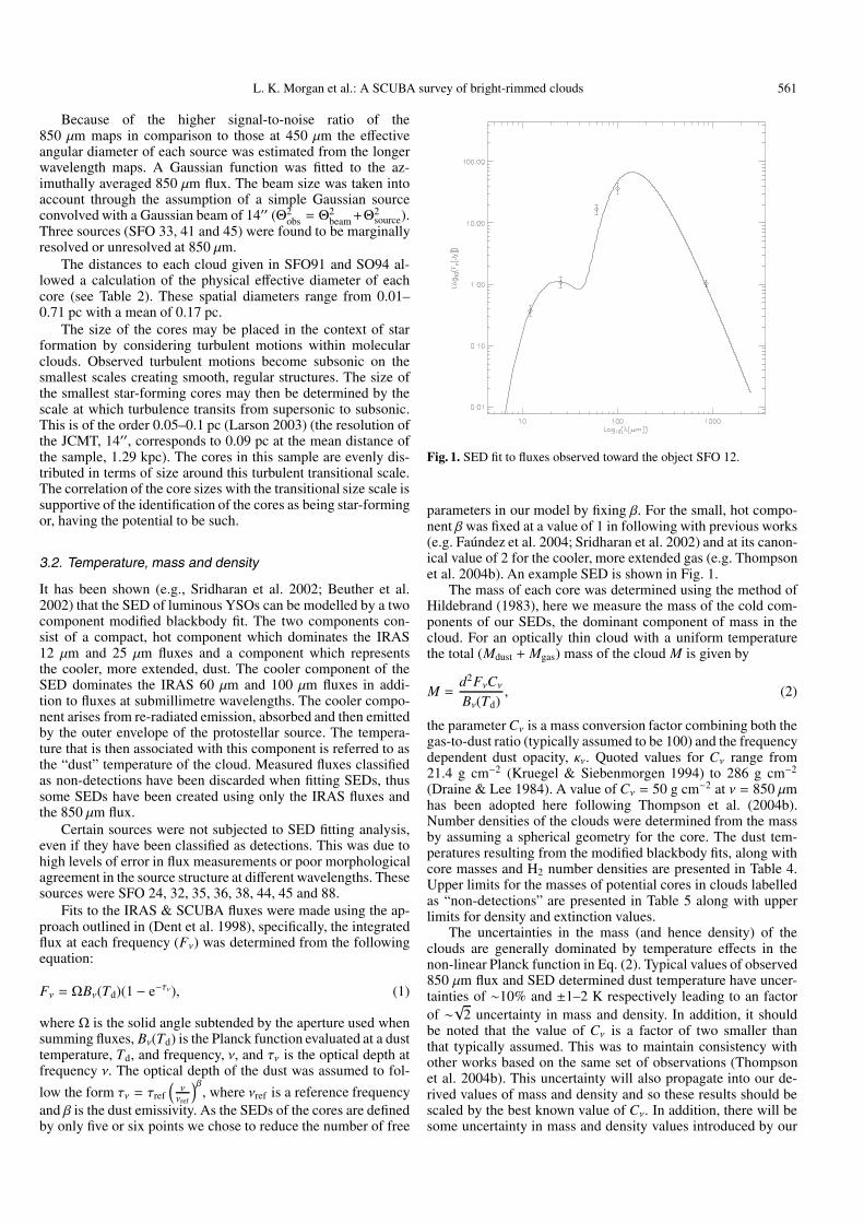
It has been shown (e.g., Sridharan et al. 2002; Beuther et al.2002) that the SED of luminous YSOs can be modelled by a twocomponent modified blackbody fit. The two components con-sist of a compact, hot component which dominates the IRAS12 µm and 25 µm fluxes and a component which representsthe cooler, more extended, dust. The cooler component of theSED dominates the IRAS 60 µm and 100 µm fluxes in addi-tion to fluxes at submillimetre wavelengths. The cooler compo-nent arises from re-radiated emission, absorbed and then emittedby the outer envelope of the protostellar source. The tempera-ture that is then associated with this component is referred to asthe “dust” temperature of the cloud. Measured fluxes classifiedas non-detections have been discarded when fitting SEDs, thussome SEDs have been created using only the IRAS fluxes andthe 850 µm flux.
Certain sources were not subjected to SED fitting analysis,even if they have been classified as detections. This was due tohigh levels of error in flux measurements or poor morphologicalagreement in the source structure at different wavelengths. Thesesources were SFO 24, 32, 35, 36, 38, 44, 45 and 88.
Fits to the IRAS & SCUBA fluxes were made using the ap-proach outlined in (Dent et al. 1998), specifically, the integratedflux at each frequency (Fν) was determined from the followingequation:
Fν = ΩBν(Td)(1 − e−τν), (1)
where Ω is the solid angle subtended by the aperture used whensumming fluxes, Bν(Td) is the Planck function evaluated at a dusttemperature, Td, and frequency, ν, and τν is the optical depth atfrequency ν. The optical depth of the dust was assumed to fol-
low the form τν = τref
(ννref
)β, where νref is a reference frequency
and β is the dust emissivity. As the SEDs of the cores are definedby only five or six points we chose to reduce the number of free
Fig. 1. SED fit to fluxes observed toward the object SFO 12.
parameters in our model by fixing β. For the small, hot compo-nent β was fixed at a value of 1 in following with previous works(e.g. Faúndez et al. 2004; Sridharan et al. 2002) and at its canon-ical value of 2 for the cooler, more extended gas (e.g. Thompsonet al. 2004b). An example SED is shown in Fig. 1.
The mass of each core was determined using the method ofHildebrand (1983), here we measure the mass of the cold com-ponents of our SEDs, the dominant component of mass in thecloud. For an optically thin cloud with a uniform temperaturethe total (Mdust + Mgas) mass of the cloud M is given by
M =d2FνCνBν(Td)
, (2)
the parameter Cν is a mass conversion factor combining both thegas-to-dust ratio (typically assumed to be 100) and the frequencydependent dust opacity, κν. Quoted values for Cν range from21.4 g cm−2 (Kruegel & Siebenmorgen 1994) to 286 g cm−2
(Draine & Lee 1984). A value of Cν = 50 g cm−2 at ν = 850 µmhas been adopted here following Thompson et al. (2004b).Number densities of the clouds were determined from the massby assuming a spherical geometry for the core. The dust tem-peratures resulting from the modified blackbody fits, along withcore masses and H2 number densities are presented in Table 4.Upper limits for the masses of potential cores in clouds labelledas “non-detections” are presented in Table 5 along with upperlimits for density and extinction values.
The uncertainties in the mass (and hence density) of theclouds are generally dominated by temperature effects in thenon-linear Planck function in Eq. (2). Typical values of observed850 µm flux and SED determined dust temperature have uncer-tainties of ∼10% and ±1–2 K respectively leading to an factorof ∼√2 uncertainty in mass and density. In addition, it shouldbe noted that the value of Cν is a factor of two smaller thanthat typically assumed. This was to maintain consistency withother works based on the same set of observations (Thompsonet al. 2004b). This uncertainty will also propagate into our de-rived values of mass and density and so these results should bescaled by the best known value of Cν. In addition, there will besome uncertainty in mass and density values introduced by our
562 L. K. Morgan et al.: A SCUBA survey of bright-rimmed clouds
uncertainty in β. This is commonly assumed to be 2 and can befairly well constrained in certain circumstances, note that onlythe cooler component of β is relevant in this case as we are onlyderiving the mass associated with this component of our sources,the majority of the mass of the system.
Values of the visual and near-infrared extinction (AV & Ak)toward each core were derived from their submillimetre fluxesfollowing the method of Mitchell et al. (2001). The submillime-tre flux Fν may be related to the visual extinction by:
Fν = ΩBν(Td)κνmHNH
E(B − V)1R
Av, (3)
where the total opacity of gas and dust is represented by κν,which is functionally equivalent to the reciprocal of the massconversion factor Cν, mH is the molecular mass of interstellarmaterial, NH/E(B − V) is the conversion factor between columndensity of hydrogen nuclei and the selective absorption at therelevant wavelength. Following Mitchell et al. (2001, and refer-ences therein) a value of NH/E(B − V) = 5.8× 1021 cm−2 mag−1
has been assumed. A value of R = 5 has been assumed in linewith predictions of the extinction of the inner regions of molec-ular clouds (e.g. Campeggio et al. 2007). The K-band extinc-tion AK of each source was found by multiplying by the ratioAV/AK = 8.9 (Rieke & Lebofsky 1985). Values of AV and AK arelisted in Table 4, along with the dust temperatures and masses,etc. derived from the submillimetre observations.
3.3. 2MASS colour-selected YSOs associated with the BRCs
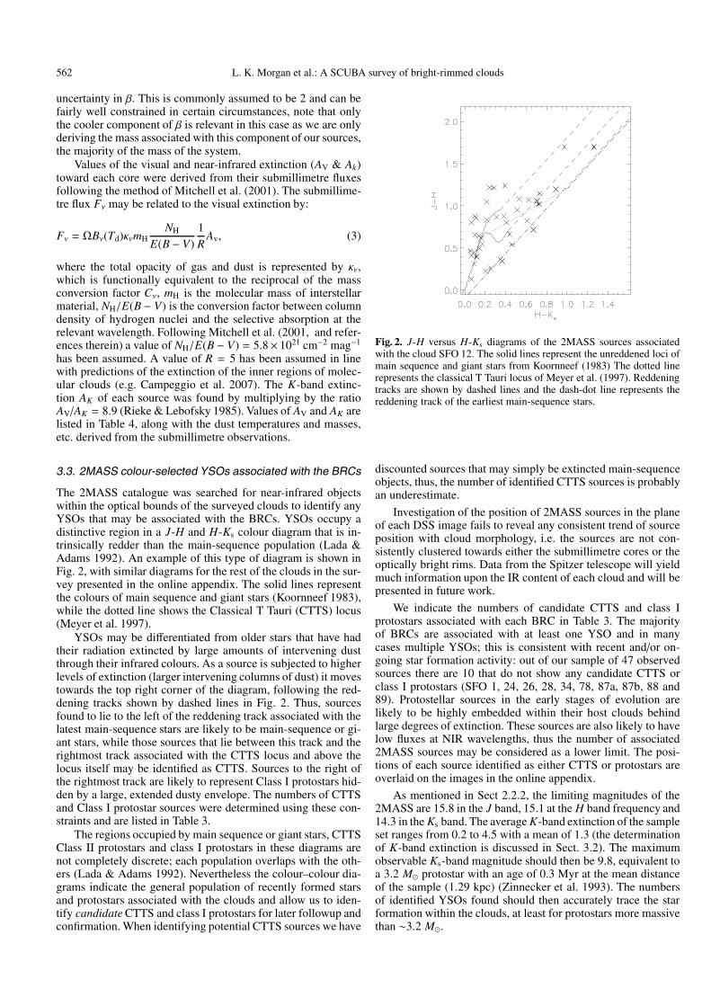
The 2MASS catalogue was searched for near-infrared objectswithin the optical bounds of the surveyed clouds to identify anyYSOs that may be associated with the BRCs. YSOs occupy adistinctive region in a J-H and H-Ks colour diagram that is in-trinsically redder than the main-sequence population (Lada &Adams 1992). An example of this type of diagram is shown inFig. 2, with similar diagrams for the rest of the clouds in the sur-vey presented in the online appendix. The solid lines representthe colours of main sequence and giant stars (Koornneef 1983),while the dotted line shows the Classical T Tauri (CTTS) locus(Meyer et al. 1997).
YSOs may be differentiated from older stars that have hadtheir radiation extincted by large amounts of intervening dustthrough their infrared colours. As a source is subjected to higherlevels of extinction (larger intervening columns of dust) it movestowards the top right corner of the diagram, following the red-dening tracks shown by dashed lines in Fig. 2. Thus, sourcesfound to lie to the left of the reddening track associated with thelatest main-sequence stars are likely to be main-sequence or gi-ant stars, while those sources that lie between this track and therightmost track associated with the CTTS locus and above thelocus itself may be identified as CTTS. Sources to the right ofthe rightmost track are likely to represent Class I protostars hid-den by a large, extended dusty envelope. The numbers of CTTSand Class I protostar sources were determined using these con-straints and are listed in Table 3.
The regions occupied by main sequence or giant stars, CTTSClass II protostars and class I protostars in these diagrams arenot completely discrete; each population overlaps with the oth-ers (Lada & Adams 1992). Nevertheless the colour–colour dia-grams indicate the general population of recently formed starsand protostars associated with the clouds and allow us to iden-tify candidate CTTS and class I protostars for later followup andconfirmation. When identifying potential CTTS sources we have
Fig. 2. J-H versus H-Ks diagrams of the 2MASS sources associatedwith the cloud SFO 12. The solid lines represent the unreddened loci ofmain sequence and giant stars from Koornneef (1983) The dotted linerepresents the classical T Tauri locus of Meyer et al. (1997). Reddeningtracks are shown by dashed lines and the dash-dot line represents thereddening track of the earliest main-sequence stars.
discounted sources that may simply be extincted main-sequenceobjects, thus, the number of identified CTTS sources is probablyan underestimate.
Investigation of the position of 2MASS sources in the planeof each DSS image fails to reveal any consistent trend of sourceposition with cloud morphology, i.e. the sources are not con-sistently clustered towards either the submillimetre cores or theoptically bright rims. Data from the Spitzer telescope will yieldmuch information upon the IR content of each cloud and will bepresented in future work.
We indicate the numbers of candidate CTTS and class Iprotostars associated with each BRC in Table 3. The majorityof BRCs are associated with at least one YSO and in manycases multiple YSOs; this is consistent with recent and/or on-going star formation activity: out of our sample of 47 observedsources there are 10 that do not show any candidate CTTS orclass I protostars (SFO 1, 24, 26, 28, 34, 78, 87a, 87b, 88 and89). Protostellar sources in the early stages of evolution arelikely to be highly embedded within their host clouds behindlarge degrees of extinction. These sources are also likely to havelow fluxes at NIR wavelengths, thus the number of associated2MASS sources may be considered as a lower limit. The posi-tions of each source identified as either CTTS or protostars areoverlaid on the images in the online appendix.
As mentioned in Sect 2.2.2, the limiting magnitudes of the2MASS are 15.8 in the J band, 15.1 at the H band frequency and14.3 in the Ks band. The average K-band extinction of the sampleset ranges from 0.2 to 4.5 with a mean of 1.3 (the determinationof K-band extinction is discussed in Sect. 3.2). The maximumobservable Ks-band magnitude should then be 9.8, equivalent toa 3.2 M protostar with an age of 0.3 Myr at the mean distanceof the sample (1.29 kpc) (Zinnecker et al. 1993). The numbersof identified YSOs found should then accurately trace the starformation within the clouds, at least for protostars more massivethan ∼3.2 M.

L. K. Morgan et al.: A SCUBA survey of bright-rimmed clouds 563
Table 3. Numbers of class I protostellar candidates (CI) or candidate T Tauri stars (CTTS) identified from the JHKs diagrams (online appendix)for all sources.
Source Number of Number of Source Number of Number ofassociated CTTS associated CI associated CTTS associated CI
01 0 0 30 2 102 3 10 31 1 003 0 1 32 0 204 0 2 33 0 205 2 1 34 0 006a 0 6 35 0 307 0 4 36 0 309 0 1 37 0 410 0 2 38 1 312 4 3 39 0 813 1 3 40 0 214 1 9 41 0 215 0 1 42 0 116 0 3 43 1 217a 1 0 44 1 218 0 2 45 1 323 0 2 77a 0 124 0 0 78a 0 025 2 3 87a 0 026 0 0 87b 0 027 4 2 88 0 028a 0 0 89 0 029 1 1
a Non-detections at SCUBA wavelengths.
3.4. Additional IR information
In addition to the IRAS data presented in our SED analysesand the 2MASS fluxes utilised in Sect. 3.3, infrared observa-tions have been performed of large areas of the sky by both theMidcourse Space Experiment (MSX) and the Spitzer telescope.Searches were performed for observational data relevant to oursources in both the MSX and the publically available GalacticLegacy Infrared midplane Survey Extraordinaire (GLIMPSE)catalogues. Only one source from our sample was found to liewithin the field observed by GLIMPSE, which covered only thecentral two degrees in latitude of the Galaxy. This source wasSFO 30 and will be the subject of a more detailed study by theauthors in the future. Many of our sources were found to havebeen observed at 24 µm in proprietary Spitzer programmes andthese data were examined for evidence of protostellar contentwithin our sample. A total of 37 multiband imaging photometerfor Spitzer (MIPS) maps were obtained from the Spitzer archive,covering sources from the SFO catalogue. Of the sources cov-ered by these maps four (SFO 8, 19, 21 and 22) were not ob-served by the reported SCUBA observations and an additionaltwo (SFO 6 and 17) were non-detections in the SCUBA sur-vey. Of the remaining 31 sources, 25 show 24 µm emissionclearly associated with the SCUBA cores identified in Sect. 3.1.The other six clouds appear to have non-correlated 24 µm and850 µm emission.
The correlation of 24 µm emission with the positions of thereported 850 µm cores highly supports the identification of thesecores as star-forming. This includes cores in which no 2MASSYSO sources were identified (Sect. 2.2.2), these sources areSFO 01, 24, 34 and 88. The non-detection of these cores by the2MASS is most likely due to these sources being at early stagesof their evolution as described in Sect. 2.2.2. A more detailed
analysis of the publicly available Spitzer archival data is under-way by the authors and will be reported in a future work.
Several of our sources were found to contain objects identi-fied in the MSX survey. However, a very limited number of thesesources were found to be closely associated with the submillime-ter cores identified in this work (the criterion being a positionwithin one IRAS beam-width). An even smaller number of thesesources were found to have reliable fluxes within the MSX cat-alogue. Sources with flux qualities of lower than a 5-sigma de-tection were rejected. After applying these criteria, sources werefound associated with SFO 5, SFO 31, SFO 39 and SFO 43.
Fluxes from the C and E bands of the MSX survey were plot-ted upon the SEDs of the relevant sources (SEDs for SFO 31and SFO 39b are shown in Fig. 3). These fluxes (found at wave-lengths of 12.13 and 21.34 µm) serve as a useful comparisonto our IRAS HiRes fluxes, found in Sect. 2.2.1. The SEDs showthat MSX fluxes largely agree with the IRAS HiRes fluxes foundat similar wavelengths for three of the five sources found to haverelevant detections in the MSX survey, given the errors inherentin comparing the two surveys. This similarity is exemplified bythe source SFO 31, shown in Fig. 3. Attention may be drawnto the two sources within which fluxes were not in such goodagreement. SFO 39a and 39b show rather large disagreement be-tween the MSX-derived fluxes and the line of the SED as drawnby our best-fit method. It should be noted that these objects arefairly poorly fit in our SED analysis and that the IRAS HiRes60 µm point is also discrepant with the line. A possible explana-tion for this is that the source is known to comprise at least twodistinct sources and so there may be “blending” of the sourceemission in at least the IRAS beam if not the SCUBA beam. Asfurther Spitzer data is released, the quality of NIR measurementsof these sources will allow a great improvement in the fitting ofthese sources’ SEDs at shorter wavelengths.

564 L. K. Morgan et al.: A SCUBA survey of bright-rimmed clouds
Fig. 3. SEDs of the sources SFO 31 (left) and SFO 39b (right) including fluxes from the MSX survey. MSX fluxes are shown as error bars only,IRAS and SCUBA fluxes are plotted as diamonds.
Fig. 4. SCUBA 850 µm contours overlaid on DSS images of SFO 13.Triangles indicate infrared sources from the 2MASS Point SourceCatalogue (Cutri et al. 2003) that have been identified as YSOs.Contours start at 6σ and increase in increments of 20% of the peakflux.
4. Analysis
4.1. Cloud morphology
The SCUBA images of the cloud sample show submillimetrecores generally located immediately behind the optically brightrims (online appendix). The submillimetre core positions aregenerally consistent with the IRAS source positions presentedin SFO91 and SO94 (i.e. the submillimetre cores lie within theIRAS beam “footprint”), though some discrepancy may be dueto the IRAS tracing the more diffuse dust surrounding the cores.
The submillimetre emission from each core is approximatelyradially symmetric at the 50% level. Below the 50% flux levelthe weaker, more diffuse, submillimetre emission from eachsource generally follows the optical boundaries of the brightrimmed clouds and thus may show a cometary morphology(e.g. SFO 13, Fig. 4). A general summary of morphology isthen: radially symmetric contours surrounded by diffuse emis-sion following the optical cloud morphology and often elongated
Fig. 5. SCUBA 850 µm contours overlaid on DSS images of SFO 12.Triangles indicate infrared sources from the 2MASS Point SourceCatalogue (Cutri et al. 2003) that have been identified as YSOs.Contours start at 4σ and increase in increments of 20% of the peakflux.
along the direction of the ionising source, exemplified by SFO12 in Fig. 5.
4.2. Luminosities of embedded sources
Use of the far infrared (FIR) and submillimetre fluxes of thesources allows the estimation of the spectral class of any YSOsthat may be present in the cloud cores. The luminosities of eachsource were estimated by integrating under the modified black-body curve fitted to each cloud’s observed fluxes, as presentedin Table 4. Distances to each source were taken from SFO91 andSO94. The derived properties of the internal sources are pre-sented in Table 4, upper flux limits from those sources that werenot detected by the survey have been utilised to determine upperlimits for the masses of potential cores in those clouds, alongwith upper limits for density and extinction values. These valuesare presented in Table 5.
The assumption has been made in this analysis that all FIRand submillimetre luminosity is due to a single source, enabling

L. K. Morgan et al.: A SCUBA survey of bright-rimmed clouds 565
Table 4. Core properties determined from modified blackbody fits.
DistanceSource THot TCold M Log10 (n) AV AK Luminosity Spectral to cloudb Lsubmm/Lbol
(K) (K) (M) cm−3 (L) typea (kpc) (×10−3)01 169 26 2.18 4.6 8.5 1.0 122 B8 0.85 6.902 182 22 3.37 4.8 13.2 1.5 57 B9 0.85 15.503 126 24 1.15 4.3 4.5 0.5 39 A0 0.85 9.204 182 26 0.03 4.6 2.1 0.2 1 G2 0.19 6.705 107 24 25.85 4.6 20.2 2.3 1154 B4 1.90 6.507 170 21 31.26 4.7 24.4 2.7 400 B5 1.90 19.009 185 27 3.03 3.7 2.4 0.3 181 B7 1.90 6.510 181 29 2.22 3.5 1.7 0.2 268 B6 1.90 4.012 157 21 16.87 4.4 13.2 1.5 201 B7 1.90 18.513 177 23 19.60 4.5 15.3 1.7 444 B5 1.90 11.514 121 27 51.79 4.9 40.5 4.5 3205 B2 1.90 5.815 130 25 7.04 3.3 1.7 0.2 317 B6 3.40 7.316 60 17 1.25 5.3 22.1 2.5 8 A8 0.40 24.418 108 18 1.15 5.3 20.3 2.3 6 F0 0.40 30.623 125 19 6.26 4.2 6.9 0.8 40 A0 1.60 27.125a 139 19 5.59 5.1 25.9 2.9 43 A0 0.78 24.325b 139 19 5.69 5.1 26.4 3.0 43 A0 0.78 24.626 212 24 1.05 3.9 2.2 0.3 28 A1 1.15 10.227 153 24 3.36 4.4 7.2 0.8 108 B8 1.15 9.929 219 22 3.57 4.4 7.6 0.9 48 A0 1.15 14.530 127 34 29.33 4.5 17.1 1.9 6945 B1.5 2.20 2.331 147 27 1.19 4.1 3.4 0.4 96 B8 1.00 5.333 149 24 0.45 4.1 2.2 0.3 21 A2 0.75 10.034 188 21 1.55 4.6 7.8 0.9 23 A2 0.75 15.737 127 20 3.82 5.0 19.2 2.2 63 B9 0.75 12.539a 133 20 2.77 4.9 13.9 1.6 36 A0 0.75 16.339b 134 21 2.09 4.7 10.5 1.2 35 A0 0.75 13.140 224 24 0.45 4.1 2.2 0.3 16 A4 0.75 9.441 189 24 0.43 4.0 2.1 0.2 15 A4 0.75 8.542 187 22 0.89 4.4 4.5 0.5 16 A4 0.75 12.343 143 26 28.34 4.4 13.9 1.6 1385 B3 2.40 6.187a 204 30 5.93 4.4 8.8 1.0 698 B4 1.38 4.087b 204 31 4.45 4.3 6.6 0.7 657 B4 1.38 3.489 194 30 5.18 4.3 7.7 0.9 597 B5 1.38 4.1
a Spectral types taken from De Jager & Nieuwenhuijzen (1987).b Distances taken from Sugitani et al. (1991) and Sugitani & Ogura (1994).
Table 5. Limiting values of potential core properties determined fromupper flux limits in the survey’s non-detections.
Source M Log10 (n) AV AK
(M) cm−3
06 7.80 4.1 6.1 0.717 0.32 4.7 5.6 0.628 1.95 4.1 4.2 0.577 2.48 3.8 2.6 0.378 2.89 3.8 3.0 0.3
an order of magnitude estimate of the stellar content within theprotostellar envelope. Wood & Churchwell (1989) showed that,for a realistic mass function, the spectral type of the most mas-sive member in a cluster is only 1.5–2 spectral classes lower thanthat derived for the single embedded star case. The median lumi-nosity of internal sources in the sample is ∼63 L, correspondingto a spectral type of B9.
4.3. Classification of the internal sources
Andre et al. (1993) defined Class 0 protostars as those obey-ing the approximate relationship Lsubmm/Lbol 5 × 10⁻³ (herewe adopted the definition of Lsubmm as the luminosity radiated
longward of 350 µm). The clouds that have been modelled us-ing the modified blackbody analysis all approximately obeythis relationship (see Table 4) with 29 of 34 sources havingLsubmm/Lbol ≥ 5 × 10⁻³ and all sources having Lsubmm/Lbol ≥2.3 × 10⁻³. No correlation was found between the masses, lu-minosities or temperatures of the sources and the value of theirLsubmm/Lbol ratio.
The dust temperatures that have been found for the cores inthe sample presented here are higher than that normally foundfor starless cores (Td ∼ 10 K, Evans 1999). This is expectedas internal hot components are observed, these are heating theprotostellar cores from within, and this establishes a scenario ofongoing star formation within our sample.
The bolometric luminosities derived for the clouds in thissurvey range from 1 L, typical of class 0 and class I protostellarobjects (Andre et al. 1993; Chandler & Richer 2000), to 6945 L,more indicative of massive star formation (Mueller et al. 2002).The median luminosity found for the sample is ∼63 L. Thissuggests that the sample consists largely of intermediate-massstar forming regions or stellar clusters, consistent with the find-ings of SFO91 and Yamaguchi et al. (1999). This is despite thedifferences in fluxes found between the IRAS PSC fluxes usedby SFO91 and IRAS HiRes fluxes used here.

566 L. K. Morgan et al.: A SCUBA survey of bright-rimmed clouds
4.4. Cloud classification
SFO91 separated their catalogue into three morphological typesbased upon the curvature exhibited by the BRC. Their classifi-cations are as follows, (1) type A, moderately curved rim witha length to width ratio, l/w, of less than 0.5; (2) type B, tightlycurved rim with l/w greater than 0.5 and; (3) type C, cometaryrim5.
The three rim types are closely related to the developmentof clouds under the influence of ionising sources. The three gen-eral rim types, A, B and C, closely match the Lefloch & Lazareff(1994) RDI model snapshots at 0.036, 0.126 and 1.3 Myr re-spectively. This strongly suggests that the variation in the largescale morphology represents the duration of each clouds expo-sure to ionising radiation, rather than a fundamental differencein structure or composition. This is further supported by the factthat Lefloch & Lazareff (1994) found no significant effects uponthe morphological evolution of the clouds due to varying initialconditions.
A simplistic interpretation of the results of Lefloch &Lazareff (1994) is that, if their evolutionary scenario is correct,then the fractional number of type “A”, “B” and “C” type rimsobserved should match the fractional lifetime of each phase.This was found not to be the case, however. The simulationsof Miao et al. (2006) have reproduced the morphological resultsof Lefloch & Lazareff (1994) but incorporate self-gravity andthermal evolution into their models. Whilst Miao et al. (2006)find a similar morphological evolution to Lefloch & Lazareff(1994) they find that the inclusion of self-gravity decreases thetimescale for the cometary morphology of their simulated cloudsto develop. The simulations of Kessel-Deynet & Burkert (2003)include the effects of self-gravity as well as ionisation. Thesesimulations similarly show decreased timescales for morpholog-ical evolution in comparison to the results of Lefloch & Lazareff(1994). They also show fragmentation occuring in BRCs oncea type “C” morphology has been achieved (on a timescale of∼0.4 Myr) and subsequently show small “trunk-like” structuresemerging from the larger BRC.
Miao et al. (2006) gives representative ages for the “A”, “B”and “C” type rims of 0.24, 0.30 and 0.39 Myr respectively. Usingthe results of Miao et al. (2006) a close match was found be-tween the number of “A” type rims classified in the SFO cata-logue and the lifetime of each of these phases (63% predictedcompared to 66% observed). If the variation in rim morphologyseen across the SFO catalogue may then be attributed to an evo-lutionary sequence then it is reasonable to search for differencesin the physical properties of the different rim types. It is expectedthat the core properties such as temperature and density wouldincrease with time, while the mass of the cold component woulddecrease as the protostellar envelope is accreted onto the centralobject and the cloud is further evaporated by the ionising UV ra-diation. One would naively expect to find star formation that ismore developed in the clouds that are further evolved.
The morphological types of each BRC as identified bySFO91 are tabulated in Table 2. It can be seen that the numberof “A” type clouds exceeds the number of “B” types by approx-imately a factor of 2 (26 as compared to 14) with only 2 “C”type rims. While the timescales reported for “A” type rims ver-sus the total of “B” and “C” type rim timescales in Miao et al.(2006) match those observed, the lack of observed “C” type rims
5 SFO 36 was identified by SFO91 as “A or C’. Based upon the posi-tion and morphology of the submillimetre emission presented in theseimages the identification of SFO 36 as type “A” morphology is evident(see Fig. 6).
Fig. 6. SCUBA 850 µm contours overlaid on DSS images of SFO 36.Triangles indicate infrared sources from the 2MASS Point SourceCatalogue (Cutri et al. 2003) that have been identified as YSOs.Contours start at 9σ and increase in increments of 20% of the peakflux.
Table 6. Mean core properties grouped as rim type. Values in parenthe-ses are the standard deviation over the sample.
Rim type THot TCold M Log10 (n) Ak
(K) (K) (M) cm−3
A 165 (45) 24 (4) 5.4 (12.5) 4.8 (0.5) 1.1 (1.1)B 157 (29) 24 (4) 11.7 (11.5) 5.0 (0.4) 1.5 (0.9)C 127 (1) 22 (3) 2.5 (1.9) 5.2 (0.5) 1.4 (1.2)
is unexplained. Given the large amount of time attributed to thisphase by Lefloch & Lazareff (1994) many of these type rimsshould be observed. However, without more detailed informa-tion on the modelling of the eventual fate of these clouds, it isnot possible to draw any conclusions about the lack of observed“C” type rims.
Grouping the cores in the sample according to the classifi-cations of SFO91 (Table 6) does not show any significant dif-ferences in the derived core properties (e.g. mass, density andextinction) between the “A” rims and the “B” rims. This is notwhat might be expected if the rim types are indeed an evolution-ary sequence. This suggests two possible scenarios.
1. The timescale for the development of rim type is short com-pared to star formation. Thus, assuming that the stars areformed as a result of the interaction of the ionisation frontwith the BRC, these stars begin to form quickly as a resultof this influence. The clouds then rapidly evolve through thesuggested development of rim type irrespective of the stateof star formation within them.
2. The formation of stars within the BRCs is unrelated to theinteraction of the ionisation front with the BRC. In this casethe development of stars within the clouds would be uncon-nected to the wider cloud evolution.

L. K. Morgan et al.: A SCUBA survey of bright-rimmed clouds 567
Table 7. Comparison of cloud properties between those with and thosewithout associated radio emission, values in parentheses represent thestandard deviation within the group.
IBL detectiona IBL non-detectionSource property Mean value Mean value
THot (K) 154 (38) 157 (34)TCold (K) 24 (4) 23 (3)
Core mass (M) 11 (14) 2 (2)Log density 5.0 (0.5) 4.8 (0.4)
Ak 1.5 (1.2) 0.7 (0.5)NCI
b 3 (2) 3 (3)NCTTS 1 (1) 0
Lbol (L) 651 (1547) 50 (53)Lsubmm/Lbol 12e-03 (7.7e−03) 14e−03 (6.4e−03)
a Detection at 21cm; b CI = Class I protostellar source.
4.5. Radio detections and ionising stars
Morgan et al. (2004) used archival NVSS (Condon et al. 1998)data to look for radio emission from the northern SFO cata-logue. Of the 44 clouds observed here, 39 were observed and31 detected by the NVSS (All of the northern sources that havebeen observed with SCUBA here were included in Morgan et al.2004). All but one of these detections was classified as an ionisedboundary layer (IBL) at the edge of the respective bright rim, es-tablishing the interaction of the HII region with the surroundingmolecular material. The number of sources with a clearly definedIBL demonstrates that ∼70% of these BRCs are being influencedby the expansion of their respective ionisation fields. Here wefind eight clouds in which we have detected submillimetre emis-sion, associated with a prospective protostellar core, which showno detectable radio emission. These clouds are SFO 3, 9, 23, 24,26, 33, 34 and 39.
If an interaction between the ionising source and the molec-ular material exists in the eight clouds not detected at ∼21 cm,then it is presumably at a much lower level than in the rest ofthe sample. A comparison between these two sets of sources istherefore warranted to search for differences which may high-light the presence and/or effects of RDI. The mean temperatures,masses, densities, extinctions, luminosities, internal stellar con-tents and the degree of IR source association of the two sets werecompared (Table 7). Clouds without associated radio emissionshow a tendency towards lower mass, density, visual extinctionand luminosity, though this tendency must be dealt with cau-tiously due to the size of the standard deviations within the re-spective groups. It can be seen from Table 7 that all values agreewithin these standard deviations. A tentative statement is then,the presence of a strong ionisation field in the vicinity of proto-stars taken from the observed sample may lead to more massive,luminous protostellar sources. Support for this statement may befound by comparing the distribution of source mass for thosesources detected and not-detected at radio wavelengths. Figure 7shows a histogram of both sets of sources, it can be seen thatthe distribution of those sources detected at radio wavelengthscontains a noticeably higher number of higher mass sources.
If there exists a correlation between the radio flux emanatingfrom a source rim and the mass/luminosity of the internal proto-star embedded within that rim then it is warranted to compare theluminosities and masses of each source to the predicted ionisingflux of each rim’s ionising source, i.e. the ionising flux we expectto be arriving at each cloud’s rim given the spectral type of thestar powering the related HII region and the projected distancebetween that star and the observed bright rim.
Fig. 7. Histogram plot of the mass distributions of those sources bothdetected (filled) and not detected (black line) in the 21 cm NVSS.
Fig. 8. Plot of the internal luminosity of protostars vs. the predicted ion-ising flux arriving at the bright rim of sources with “B” and “C” typemorphologies.
A correlation was found between the predicted ionising fluxand the luminosity of each protostellar object. Futhermore, itwas found that this correlation appeared to arise solely fromthe type “B” and type “C” rims within our sample. Type “A”rims showed no such correlation, a plot of the relation betweenthe predicted ionising flux (Morgan et al. 2004) and the inter-nal source luminosity for “B” and “C” type rims is presented inFig. 8.
It would then appear that there is a link between the strengthof the ionisation field in which the BRCs are embedded and theluminosity of stars that are produced within those clouds, at leastfor “B” and “C” type rims. This is a very good indication that,at some level, the illuminating source of the HII region plays animportant role in the formation of stars within BRCs.

568 L. K. Morgan et al.: A SCUBA survey of bright-rimmed clouds
Fig. 9. The mass spectrum of the sources detected by SCUBA in thissurvey. The Y-axis represents the cumulative number of sources (Ncum)per mass bin of size 0.05 M. The long-dash line represents the gi-ant molecular cloud clump mass function taken from Blitz (1993) andthe short-dash line represents the well-known Salpeter slope (Salpeter1955). The solid line represents a best fit to the data from the presentedsample.
4.6. The mass function of the SFO catalogue
The “Initial Mass Function” (IMF) is a key diagnostic in distin-guishing between various regimes of star formation processes.The Salpeter mass function (Salpeter 1955) describing main se-quence stars is:
dN(M)dM
∝ M−2.35. (4)
This relation has been refined in different circumstances in anattempt to describe stars that are observed to have number func-tions differing from that presented in Salpeter (1955). Blitz(1993) found an observed mass spectrum for “clumps” withinGiant Molecular Clouds (GMC) that obeys
dN(M)dM
∝ M−1.54. (5)
The masses that have been found from Eq. (2) for the detectedcores in this survey are presented in Table 4, the correspondingmass spectrum arising from this sample is presented in Fig. 9.The Salpeter and Blitz slopes are presented for comparison andhave values of −2.35 and −1.54 respectively, while a least-squares fit to our data gives a slope of −1.67.
We estimate that our sample is complete to 3σ at ∼0.5 M.Therefore, when fitting a line to the mass spectrum presentedhere we have discarded sources with derived masses below thisvalue. The usefulness of a comparison with the Salpeter slopemay not be completely valid as the Salpeter slope describesstars upon the main sequence, whereas this sample is com-prised of YSOs (or possibly multiple YSOs) which are funda-mentally different astronomical objects to main sequence stars.However, an important question is addressed by a comparison ofthe presented sample’s mass spectrum with the Salpeter slope.
Fig. 10. The luminosities of the SCUBA sample plotted as a function ofdistance (diamonds), the solid line represents the sensitivity limit of theIRAS.
Alves et al. (2007) found that the mass function of dense molec-ular cores is similar in shape to the stellar IMF but may bescaled to higher masses. Their observations of 159 dense coresrevealed a “Salpeter-like power law”. It can be seen that theslope of our mass spectrum is in fact significantly shallowerthan that of the Salpeter function and somewhat shallower thanthe Blitz “clump” function. From this, we can determine thatthese sources are more efficiently producing higher mass starsthan may be expected or, as is more likely, these sources containembedded clusters of stellar sources. This increased efficiencyis apparent at a given mass, therefore, the observed differencein slope may well be interpreted as a lack of low-mass sourcesrather than a preponderance of high-mass sources.
The sensitivity of IRAS limits the sample to sources above∼3 L at a mean distance of 1.29 kpc. By plotting the luminos-ity/distance relationship of these sources6 (Fig. 10) it can be seenthat the sample lies well above this sensitivity limit
4.6.1. Separating the sample
If, as suggested in Sect. 4.5, the protostars found within the dif-ferent cloud morphologies have some fundamental difference intheir formation mechanism then it may become more evidentby separating the sample on a morphological basis and plottingmass spectra separately.
Here we compare our source sample with data taken fromMitchell et al. (2001), in which 850 µm SCUBA maps are pre-sented of 67 discrete continuum sources in the Orion B molecu-lar cloud, some of which are shown to be star-forming. Mitchellet al. (2001) define a mass for each “clump” through assuming adust temperature, Td, via:
Mclump = 1.50×S 850
[exp
(17 KTd
)−1
]×(
κ850
0.01 cm2 g−1
)−1
M (6)
6 In creating this plot only 60 and 100 µm fluxes were used and com-pared to the flux limits of IRAS at these wavelengths.

L. K. Morgan et al.: A SCUBA survey of bright-rimmed clouds 569
Fig. 11. The mass spectrum of the “A” type (left) and “B” and “C” type (right) sources detected by SCUBA in this survey (pluses) and in the surveyof Mitchell et al. (2001) (diamonds). The Y-axis represents the log of the cumulative number of sources (Ncum) per mass bin of size 0.05 M as afraction of N, where N is the total number of sources. The solid line is a best fit to our data above the mean sensitivity limit, the dash-dot line is abest fit to the data of Mitchell et al. (2001). The outlier of SFO 14 with mass 51.79 M has been neglected from the fit for the “A” type rims as itappears anomalous, see Sect. 5.
where S 850 is the 850 µm flux enclosed within the clump bound-ary measured in Janskys and κ850 is the mass absorption coeffi-cient at 850 µm, functionally equivalent to the reciprocal of themass conversion factor Cν (see Sect. 3.2). Mitchell et al. (2001)use fluxes for each clump taken from a 21′′ aperture and as-sume a value for κ850 of 0.01 cm g−1 to find masses for a smallsample of the clumps in their survey. In order to find massesfor the complete sample of their observations we have recalcu-lated their dust masses assuming a dust temperature of 20 K.As the 850 µm fluxes within a 21′′ aperture are not available,and to maintain consistency with the method presented here, wehave used the total integrated flux along with a different value ofκ850 = 0.02 cm2 g−1. The masses found here agree well withthose presented for the smaller sample within Mitchell et al.(2001).
Plotting the mass spectrum of the clumps observed withinMitchell et al. (2001) may provide a more illuminating compar-ison to our sample than the Salpeter function, or the Blitz ob-served clump mass spectrum. As well as the protostellar clumpsbeing similar objects to this sample (the important difference be-ing the illumination of the clouds by nearby massive stars) themethods used to derive their masses are identical, whereas theSalpeter and Blitz spectra are based upon various observationsand assumptions. It should be noted that Orion B is a single dis-tance sample, while this sample represents BRCs at a range ofdistances which may not be well known. This could possibly in-troduce errors into the sample. As with our own mass spectrumlower mass sources have not been used in a best-fit slope to themass spectrum in order to reduce the effects that an incompletesample may have on the determination.
The mass spectra presented in Fig. 11 show that clouds withtype “A” morphologies appear to follow a mass function closeto that of the survey of Mitchell et al. (2001), while clouds withtype “B” and “C” morphologies have a significantly shallowermass function. It is noticeable that the best fit line to our “A” typerim mass function may be skewed by a few outliers at around 3–4 M. The number of data points in this plot is low and thuswe must try to fill in the graph around these points in order toexplore this function further. However, the suggestion from thesespectra is that “A” type rims seem to follow a mass law similarto that found in other, non-triggered regions. Whereas type “B”and type “C” rims have a significantly shallower mass spectrum,
indicating a tendency toward greater numbers of higher masssources.
5. Discussion
Our survey of the submillimetre emission found within BRCshas revealed the presence of embedded cores. The positions ofpeak submillimetre flux are consistent with IRAS PSC sources,previously discussed by SFO91, SO94 and Morgan et al. (2004)and situated near the edge of known HII regions. Morgan et al.(2004) established the presence of IBLs and photon dominatedregions (PDRs) at the interface between the HII regions andthe molecular clouds composing the BRCs. Previous studies(Morgan et al. 2004; Thompson et al. 2004b; Urquhart et al.2006, 2007) also show that many of these clouds are likely tobe in a post-shocked state and that any observed star formationis therefore a possible result of the cloud’s interaction with theexternal ionising source.
The embedded cores are likely to contain class 0 protostarswith few exceptions (29 of 34 sources obey the Andre et al. 1993,classification for class 0 protostars of Lsubmm/Lbol 5 × 10⁻³).Dust temperatures found towards the cores exceed those foundtowards starless cores (∼10 K, Evans 1999) with an averageof 24 K. This combination of observed submillimetre flux ex-cess and high dust temperatures clearly establishes a scenarioof ongoing early star formation within the sample of BRCs.Bolometric luminosities of the sources have a large range, from1 L for SFO 4 to 6945 L for SFO 30. However, the majorityof sources have Lbol > 10 L suggesting that the sample con-sists largely of intermediate to high-mass star-forming regions.Though some, if not all, of the higher luminosity sources arelikely host to protostellar clusters rather than individual proto-stars.
Bright-rimmed clouds are the potential results of RDI andit has been suggested by theoretical investigations that theymay follow a morphological evolutionary sequence (Lefloch& Lazareff 1994; Kessel-Deynet & Burkert 2003; Miao et al.2006). In this scenario different morphological classificationsmay host different classes, or epochs, of star formation. A pre-liminary analysis revealed that this was not the case. The sam-ple was separated into each morphological grouping and av-erage masses, luminosities, dust temperatures, extinctions and

570 L. K. Morgan et al.: A SCUBA survey of bright-rimmed clouds
densities were found to be similar for all sources with no signifi-cant deviations; no link between rim morphology and embeddedcore properties could be made. This strongly suggests that thedevelopment of rim type and the ongoing star formation withinthe BRCs are not linked, or that they occur upon differentialtimescales such that, once initiated, star formation proceeds in-dependently of any morphological changes occuring to the BRCas a whole.
The detection of radio free-free emission associated with alarge number of the clouds in our sample (Morgan et al. 2004)establishes the presence of IBLs at the edges of many of theseclouds. This indicates that there is some interaction occuring be-tween the clouds and their environment, even if this interactionis unconnected to the internal protostellar activity. It was foundthat clouds associated with radio-detected IBLs contain proto-stars, or protostellar clusters, with higher masses, densities andextinctions (column densities) than those not detected at radiowavelengths. This tendency was not found to be significantlylarge to definitively separate our sample and may simply be dueto skewing by a few, high-mass, sources. However, when the pre-dicted strength of the ionisation field within which the clouds aresituated was investigated it was found that a significant correla-tion exists between the strength of this field and the luminosityof the embedded protostars or protostellar clusters. Furthermore,it was found that this correlation arises solely from the “B” and“C” morphological type rims. This clearly indicates the interac-tion of the external ionisation field with star formation occuringwithin the clouds, at least in “B” and “C” morphological typerims. The absence of any similar correlation in “A” type rimsprovides reasonable evidence that these clouds are not subject toRDI triggering processes.
The evidence of interaction between ambient ionisation fieldstrength and star formation does not rule out the possibility offormation via the “collect and collapse” method proposed byElmegreen & Lada (1977). In this scenario the expanding nebulaaround the star ionising the HII region generates gravitationallyunstable, shocked layers of gas which are fragmented and havehigh masses (Whitworth et al. 1994). This mechanism is gener-ally long-lived and acts upon large scales (Zavagno et al. 2006)and is capable of producing the flat edged structures seen in “A”type rims such as SFO 41 and SFO 88 (Figs. A.32, A.39).
It appears that star formation occuring within different mor-phological types of BRC follows different formation processes.The star formation found within “B” and “C” morphological rimtypes resulting in some part from the influence of nearby massivestars, while the formation found within “A” type rims evolvespresumably independently of the environment within which theBRCs are located. This scenario contradicts the evolutionaryscenario of rim type predicted by Lefloch & Lazareff (1994),Kessel-Deynet & Burkert (2003) and Miao et al. (2006), at leastas connected to protostellar development. This inherently im-plies that any star formation occuring within “A” type rims musteither have existed before the ionisation of the rim or that anyrim ionisation occuring is not sufficiently dramatic to influenceany subsequent star formation.
In the light of the differences between “A” type rims and “B”and “C” type rims, we sought to further solidify any evidence ofthis exterior influence upon embedded star formation. An analy-sis of the mass functions of the two sub-classes of BRC revealedthat the star formation within “A” type rims follows a similarfunction to protostars found in an environment not subjected toexterior ionisation influence. However, “B” and “C” type rimsappear to follow a mass function more pre-disposed toward ahigher efficiency at higher masses (see Fig. 11). This indicates
that, in “B” and “C” type rims, relatively more massive objectsare formed than low-mass stars in comparison to the SalpeterIMF and thus may make an important contribution to the overallintermediate to high-mass stellar population.
6. Conclusions
Our main findings are as follows:
1. The SCUBA observations presented here generally showcentrally condensed cores interior to the rims of BRCs. Themorphology of the cores themselves suggests the presence ofbound condensations, indicative of star formation. The mor-phology of the larger area, incorporating the entire brightrim, is, in general, supportive of the scenario seen in RDImodels; a dense core at the head of an elongated column.Support for the interaction of multiple layers is given byobservations at multiple wavelengths i.e. radio observationstracing the hot ionised layer bordering the PDR observedin the near infrared which borders the molecular material,the dense regions of which are seen at submillimetre wave-lengths.
2. The physical properties of the submillimetre cores were de-termined using modified blackbody analyses. The dust tem-peratures found for the sources are high compared to starlesscores (average Td = 24 K), indicating the presence of inter-nal stellar sources in these clouds. Based on their Lsubmm/Lbolratio these sources are consistent with being Class 0 pro-tostars. In addition, the indicated stellar sources embeddedwithin the clouds may be classified via the hypothesis that allillumination is due to a single illuminating source. This leadsto spectral classifications of intermediate to high mass stellarsources within the cores, whether these sources are isolatedsingular sources or weaker sources, distributed in clusters.
3. Observations of mid-infrared sources taken from the 2MASSfurther support the proposed scenario of early star formationacross our sample by revealing the presence of young stars inthe vicinity of the majority (89%) of our sample. The spectraltype of the associated sources is not determinable from thecurrent data, however the observed stars are known to be inthe relatively early stages of their formation.
4. Both the mass functions and correlations of source luminos-ity with ionisation field strength suggest some fundamentaldifference between the subsets of “A” type rims and “B” and“C” type rims. It is suggested that “B” and “C” type rims rep-resent true “triggered” star formation as enabled by the RDIprocess. There is no reason to rule out the possibility that “A”type rims are also the result of triggering, though perhaps viaa different mechanism i.e. the “collect and collapse” model(Elmegreen & Lada 1977). The correlation between ionisa-tion field strength and source luminosity is highly indicativeof “B” and “C” type rims forming with at least some degreeof interaction with their UV surroundings. By increasing thesize of our sample and incorporating other BRCs that haveyet to begin their star formation this hypothesis may be in-vestigated further.
Acknowledgements. The authors would like to thank both an anonymous refereeand Malcolm Walmsley for their useful and illuminating comments. They haveimproved the quality of this work.The authors would like to thank the JCMT support staff for a pleasant and pro-ductive observing run; Helen Kirk for assistance with data reduction issues andD. J. Pisano for his insight and helpful discussions.The Digitized Sky Surveys were produced at the Space Telescope ScienceInstitute under US Government grant NAG W-2166. The images of these surveys
L. K. Morgan et al.: A SCUBA survey of bright-rimmed clouds 571
are based on photographic data obtained using the Oschin Schmidt Telescope onPalomar Mountain and the UK Schmidt Telescope. The plates were processedinto the present compressed digital form with the permission of these institu-tions.This publication makes use of data products from the Two Micron All SkySurvey, which is a joint project of the University of Massachusetts and theInfrared Processing and Analysis Center/California Institute of Technology,funded by the National Aeronautics and Space Administration and the NationalScience Foundation.This research made use of data products from the Midcourse Space Experiment.Processing of the data was funded by the Ballistic Missile Defense Organizationwith additional support from NASA Office of Space Science.This research has made use of the NASA/ IPAC Infrared Science Archive, whichis operated by the Jet Propulsion Laboratory, California Institute of Technology,under contract with the National Aeronautics and Space Administration.This research has made use of the SIMBAD database, operated at CDS,Strasbourg, FranceThis research has made use of NASA’s Astrophysics Data System.
ReferencesAlves, J., Lombardi, M., & Lada, C. J. 2007, A&A, 462, L17Andre, P., Ward-Thompson, D., & Barsony, M. 1993, ApJ, 406, 122Aumann, H. H., Fowler, J. W., & Melnyk, M. 1990, AJ, 99, 1674Bertoldi, F. 1989, ApJ, 346, 735Beuther, H., Walsh, A., Schilke, P., et al. 2002, A&A, 390, 289Blitz, L. 1993, in Protostars and Planets III, 125Campeggio, L., Strafella, F., Maiolo, B., Elia, D., & Aiello, S. 2007, ApJ, 668,
316Chandler, C. J. & Richer, J. S. 2000, ApJ, 530, 851Codella, C., Bachiller, R., Nisini, B., Saraceno, P., & Testi, L. 2001, A&A, 376,
271Condon, J. J., Cotton, W. D., Greisen, E. W., et al. 1998, AJ, 115, 1693Currie, M. J., & Berry, D. S. 2002, Starlink Project, CCLRCCutri, R. M., Skrutskie, M. F., van Dyk, S., et al. 2003, VizieR Online Data
Catalog, 2246, 0De Jager, C., & Nieuwenhuijzen, H. 1987, A&A, 177, 217Deharveng, L., Zavagno, A., & Caplan, J. 2005, A&A, 433, 565Dent, W. R. F., Matthews, H. E., & Ward-Thompson, D. 1998, MNRAS, 301,
1049Dobashi, K., Yonekura, Y., Matsumoto, T., et al. 2001, PASJ, 53, 85Draine, B. T., & Lee, H. M. 1984, ApJ, 285, 89Draper, P. W., Gray, N., & Berry, D. S. 2004, Starlink Project, CCLRCElmegreen, B. G. 1998, in Origins, ed. C. E. Woodward, J. M. Shull, & H. A.
Thronson, Jr., ASP Conf. Ser., 148, 150Elmegreen, B. G., & Lada, C. J. 1977, ApJ, 214, 725Evans, N. J. 1999, ARA&A, 37, 311Faúndez, S., Bronfman, L., Garay, G., et al. 2004, A&A, 426, 97
Hildebrand, R. H. 1983, QJRAS, 24, 267Hogerheijde, M. R., & Sandell, G. 2000, ApJ, 534, 880Holland, W. S., Robson, E. I., Gear, W. K., et al. 1999, MNRAS, 303, 659Hurt, R. L., & Barsony, M. 1996, ApJ, 460, L45Jenness, T., & Lightfoot, J. F. 2000, Starlink Project, CCLRCKessel-Deynet, O., & Burkert, A. 2003, MNRAS, 338, 545Koornneef, J. 1983, A&A, 128, 84Kruegel, E., & Siebenmorgen, R. 1994, A&A, 288, 929Lada, C. J., & Adams, F. C. 1992, ApJ, 393, 278Larson, R. B. 2003, Reports on Progress in Physics, 66, 1652Lefloch, B., & Lazareff, B. 1994, A&A, 289, 559Lefloch, B., & Lazareff, B. 1995, A&A, 301, 522Lefloch, B., Lazareff, B., & Castets, A. 1997, A&A, 324, 249Levine, D. M., & Surace, J. 1993, IPAC Users’ Guide, 5th Ed. (Pasadena: IPAC)Megeath, S. T., & Wilson, T. L. 1997, AJ, 114, 1106Meyer, M. R., Calvet, N., & Hillenbrand, L. A. 1997, AJ, 114, 288Miao, J., White, G. J., Nelson, R., Thompson, M., & Morgan, L. 2006, MNRAS,
369, 143Mitchell, G. F., Johnstone, D., Moriarty-Schieven, G., Fich, M., & Tothill,
N. F. H. 2001, ApJ, 556, 215Morgan, L. K., Thompson, M. A., Urquhart, J. S., White, G. J., & Miao, J. 2004,
A&A, 426, 535Mueller, K. E., Shirley, Y. L., Evans, N. J., & Jacobson, H. R. 2002, ApJS, 143,
469Ogura, K., Sugitani, K., & Pickles, A. 2002, AJ, 123, 2597Privett, G., Jenness, T., & Lightfoot, J. F. 1998, Starlink Project, CCLRCRieke, G. H., & Lebofsky, M. J. 1985, ApJ, 288, 618Salpeter, E. E. 1955, ApJ, 121, 161Sharpless, S. 1959, ApJS, 4, 257Sridharan, T. K., Beuther, H., Schilke, P., Menten, K. M., & Wyrowski, F. 2002,
ApJ, 566, 931Sugitani, K., & Ogura, K. 1994, ApJS, 92, 163Sugitani, K., Fukui, Y., & Ogura, K. 1991, ApJS, 77, 59Thompson, M. A., & White, G. J. 2004, A&A, 419, 599Thompson, M. A., Urquhart, J. S., & White, G. J. 2004a, A&A, 415, 627Thompson, M. A., White, G. J., Morgan, L. K., et al. 2004b, A&A, 414, 1017Urquhart, J. S., Thompson, M. A., Morgan, L. K., & White, G. J. 2004, A&A,
428, 723Urquhart, J. S., Thompson, M. A., Morgan, L. K., & White, G. J. 2006, A&A,
450, 625Urquhart, J. S., Thompson, M. A., Morgan, L. K., et al. 2007, A&A, 467, 1125Whitworth, A. P., Bhattal, A. S., Chapman, S. J., Disney, M. J., & Turner, J. A.
1994, MNRAS, 268, 291Wood, D. O. S., & Churchwell, E. 1989, ApJ, 340, 265Yamaguchi, R., Saito, H., Mizuno, N., et al. 1999, PASJ, 51, 791Zavagno, A., Deharveng, L., Comerón, F., et al. 2006, A&A, 446, 171Zinnecker, H., McCaughrean, M. J., & Wilking, B. A. 1993, in Protostars and
Planets III, ed. E. H. Levy, & J. I. Lunine, 429

L. K. Morgan et al.: A SCUBA survey of bright-rimmed clouds, Online Material p 1
Online Material

L. K. Morgan et al.: A SCUBA survey of bright-rimmed clouds, Online Material p 2
Appendix A: Description of plots and images
Data for all of the SFO clouds are presented in the followingpages. SCUBA 850 µm and 450 µm contours are overlaid onDSS images. Infrared sources from the 2MASS Point SourceCatalogue (Cutri et al. 2003) that have been identified as YSOsare shown as triangles.
J-H versus H-Ks colours of the 2MASS sources associatedwith each cloud are plotted along with a figure of the SED plotof the object composed from a best fit to various observed fluxeswhere possible. J-H versus H-Ks colour diagrams have solidlines representing the unreddened loci of main sequence and gi-ant stars from Koornneef (1983). Dotted lines represent the clas-sical T Tauri locus of Meyer et al. (1997). Reddening tracks areshown by dashed lines and the dash-dot line represents the red-dening track of the earliest main-sequence stars.

L. K. Morgan et al.: A SCUBA survey of bright-rimmed clouds, Online Material p 3
Fig. A.1. Plots and images associated with the object SFO 1. The top images show SCUBA 450 µm (left) and 850 µm (right) contours overlaid on aDSS image, infrared sources from the 2MASS Point Source Catalogue (Cutri et al. 2003) that have been identified as YSOs are shown as triangles.850 µm contours start at 4σ and increase in increments of 20% of the peak flux value, 450 µm contours start at 3σ and increase in increments of20% of the peak flux value. The bottom left plot shows the J-H versus H-Ks colours of the 2MASS sources associated with the cloud while thebottom right image shows the SED plot of the object composed from a best fit to various observed fluxes.

L. K. Morgan et al.: A SCUBA survey of bright-rimmed clouds, Online Material p 4
Fig. A.2. Plots and images associated with the object SFO 2. The top images show SCUBA 450 µm (left) and 850 µm (right) contours overlaid on aDSS image, infrared sources from the 2MASS Point Source Catalogue (Cutri et al. 2003) that have been identified as YSOs are shown as triangles.850 µm contours start at 9σ and increase in increments of 20% of the peak flux value, 450 µm contours start at 5σ and increase in increments of20% of the peak flux value. The bottom left plot shows the J-H versus H-Ks colours of the 2MASS sources associated with the cloud while thebottom right image shows the SED plot of the object composed from a best fit to various observed fluxes.

L. K. Morgan et al.: A SCUBA survey of bright-rimmed clouds, Online Material p 5
Fig. A.3. Plots and images associated with the object SFO 3. The top image shows SCUBA 850 µm contours overlaid on a DSS image, infraredsources from the 2MASS Point Source Catalogue (Cutri et al. 2003) are shown as triangles. 850 µm contours start at 3σ and increase in incrementsof 20% of the peak flux value. The bottom left plot shows the J-H versus H-Ks colours of the 2MASS sources associated with the cloud while thebottom right image shows the SED plot of the object composed from a best fit to various observed fluxes.

L. K. Morgan et al.: A SCUBA survey of bright-rimmed clouds, Online Material p 6
Fig. A.4. Plots and images associated with the object SFO 4. The top images show SCUBA 450 µm (left) and 850 µm (right) contours overlaid on aDSS image, infrared sources from the 2MASS Point Source Catalogue (Cutri et al. 2003) that have been identified as YSOs are shown as triangles.850 µm contours start at 4σ and increase in increments of 20% of the peak flux value, 450 µm contours start at 5σ and increase in increments of20% of the peak flux value. The bottom left plot shows the J-H versus H-Ks colours of the 2MASS sources associated with the cloud while thebottom right image shows the SED plot of the object composed from a best fit to various observed fluxes.

L. K. Morgan et al.: A SCUBA survey of bright-rimmed clouds, Online Material p 7
Fig. A.5. Plots and images associated with the object SFO 5. The top images show SCUBA 450 µm (left) and 850 µm (right) contours overlaid on aDSS image, infrared sources from the 2MASS Point Source Catalogue (Cutri et al. 2003) that have been identified as YSOs are shown as triangles.850 µm contours start at 6σ and increase in increments of 20% of the peak flux value, 450 µm contours start at 3σ and increase in increments of20% of the peak flux value. The bottom left plot shows the J-H versus H-Ks colours of the 2MASS sources associated with the cloud while thebottom right image shows the SED plot of the object composed from a best fit to various observed fluxes.

L. K. Morgan et al.: A SCUBA survey of bright-rimmed clouds, Online Material p 8
Fig. A.6. Plots and images associated with the object SFO 7. The top images show SCUBA 450 µm (left) and 850 µm (right) contours overlaid on aDSS image, infrared sources from the 2MASS Point Source Catalogue (Cutri et al. 2003) that have been identified as YSOs are shown as triangles.850 µm contours start at 3σ and increase in increments of 20% of the peak flux value, 450 µm contours start at 3σ and increase in increments of20% of the peak flux value. The bottom left plot shows the J-H versus H-Ks colours of the 2MASS sources associated with the cloud while thebottom right image shows the SED plot of the object composed from a best fit to various observed fluxes.

L. K. Morgan et al.: A SCUBA survey of bright-rimmed clouds, Online Material p 9
Fig. A.7. Plots and images associated with the object SFO 9. The top images show SCUBA 450 µm (left) and 850 µm (right) contours overlaid on aDSS image, infrared sources from the 2MASS Point Source Catalogue (Cutri et al. 2003) that have been identified as YSOs are shown as triangles.850 µm contours start at 6σ and increase in increments of 20% of the peak flux value, 450 µm contours start at 3σ and increase in increments of20% of the peak flux value. The bottom left plot shows the J-H versus H-Ks colours of the 2MASS sources associated with the cloud while thebottom right image shows the SED plot of the object composed from a best fit to various observed fluxes.

L. K. Morgan et al.: A SCUBA survey of bright-rimmed clouds, Online Material p 10
Fig. A.8. Plots and images associated with the object SFO 10. The top image shows 850 µm contours overlaid on a DSS image, infrared sourcesfrom the 2MASS Point Source Catalogue (Cutri et al. 2003) are shown as triangles. 850 µm contours start at 3σ and increase in increments of 20%of the peak flux value. The bottom left plot shows the J-H versus H-Ks colours of the 2MASS sources associated with the cloud while the bottomright image shows the SED plot of the object composed from a best fit to various observed fluxes.

L. K. Morgan et al.: A SCUBA survey of bright-rimmed clouds, Online Material p 11
Fig. A.9. Plots and images associated with the object SFO 12. The top images show SCUBA 450 µm (left) and 850 µm (right) contours overlaidon a DSS image, infrared sources from the 2MASS Point Source Catalogue (Cutri et al. 2003) that have been identified as YSOs are shown astriangles. 850 µm contours start at 4σ and increase in increments of 20% of the peak flux value, 450 µm contours start at 3σ and increase inincrements of 20% of the peak flux value. The bottom left plot shows the J-H versus H-Ks colours of the 2MASS sources associated with thecloud while the bottom right image shows the SED plot of the object composed from a best fit to various observed fluxes.

L. K. Morgan et al.: A SCUBA survey of bright-rimmed clouds, Online Material p 12
Fig. A.10. Plots and images associated with the object SFO 13. The top images show SCUBA 450 µm (left) and 850 µm (right) contours overlaidon a DSS image, infrared sources from the 2MASS Point Source Catalogue (Cutri et al. 2003) that have been identified as YSOs are shown astriangles. 850 µm contours start at 6σ and increase in increments of 20% of the peak flux value, 450 µm contours start at 3σ and increase inincrements of 20% of the peak flux value. The bottom left plot shows the J-H versus H-Ks colours of the 2MASS sources associated with thecloud while the bottom right image shows the SED plot of the object composed from a best fit to various observed fluxes.

L. K. Morgan et al.: A SCUBA survey of bright-rimmed clouds, Online Material p 13
Fig. A.11. Plots and images associated with the object SFO 14. The top images show SCUBA 450 µm (left) and 850 µm (right) contours overlaidon a DSS image, infrared sources from the 2MASS Point Source Catalogue (Cutri et al. 2003) that have been identified as YSOs are shown astriangles. 850 µm contours start at 15σ and increase in increments of 20% of the peak flux value, 450 µm contours start at 3σ and increase inincrements of 20% of the peak flux value. The bottom left plot shows the J-H versus H-Ks colours of the 2MASS sources associated with thecloud while the bottom right image shows the SED plot of the object composed from a best fit to various observed fluxes.

L. K. Morgan et al.: A SCUBA survey of bright-rimmed clouds, Online Material p 14
Fig. A.12. Plots and images associated with the object SFO 15. The top image shows SCUBA 850 µm contours overlaid on a DSS image, infraredsources from the 2MASS Point Source Catalogue (Cutri et al. 2003) are shown as triangles. 850 µm contours start at 3σ and increase in incrementsof 20% of the peak flux value. The bottom left plot shows the J-H versus H-Ks colours of the 2MASS sources associated with the cloud while thebottom right image shows the SED plot of the object composed from a best fit to various observed fluxes.

L. K. Morgan et al.: A SCUBA survey of bright-rimmed clouds, Online Material p 15
Fig. A.13. Plots and images associated with the object SFO 16. The top images show SCUBA 450 µm (left) and 850 µm (right) contours overlaidon a DSS image, infrared sources from the 2MASS Point Source Catalogue (Cutri et al. 2003) that have been identified as YSOs are shown astriangles. 850 µm contours start at 9σ and increase in increments of 20% of the peak flux value, 450 µm contours start at 4σ and increase inincrements of 20% of the peak flux value. The bottom left plot shows the J-H versus H-Ks colours of the 2MASS sources associated with thecloud while the bottom right image shows the SED plot of the object composed from a best fit to various observed fluxes.

L. K. Morgan et al.: A SCUBA survey of bright-rimmed clouds, Online Material p 16
Fig. A.14. Plots and images associated with the object SFO 18. The top images show SCUBA 450 µm (left) and 850 µm (right) contours overlaidon a DSS image, infrared sources from the 2MASS Point Source Catalogue (Cutri et al. 2003) that have been identified as YSOs are shown astriangles. 850 µm contours start at 9σ and increase in increments of 20% of the peak flux value, 450 µm contours start at 4σ and increase inincrements of 20% of the peak flux value. The bottom left plot shows the J-H versus H-Ks colours of the 2MASS sources associated with thecloud while the bottom right image shows the SED plot of the object composed from a best fit to various observed fluxes.

L. K. Morgan et al.: A SCUBA survey of bright-rimmed clouds, Online Material p 17
Fig. A.15. Plots and images associated with the object SFO 23. The top images show SCUBA 450 µm (left) and 850 µm (right) contours overlaidon a DSS image, infrared sources from the 2MASS Point Source Catalogue (Cutri et al. 2003) that have been identified as YSOs are shown astriangles. 850 µm contours start at 3σ and increase in increments of 20% of the peak flux value, 450 µm contours start at 3σ and increase inincrements of 20% of the peak flux value. The bottom left plot shows the J-H versus H-Ks colours of the 2MASS sources associated with thecloud while the bottom right image shows the SED plot of the object composed from a best fit to various observed fluxes.
Fig. A.16. Plots and images associated with the object SFO 24. The left image shows SCUBA 850 µm contours overlaid on a DSS image, infraredsources from the 2MASS Point Source Catalogue (Cutri et al. 2003) are shown as triangles. 850 µm contours start at 3σ and increase in incrementsof 20% of the peak flux value The right plot shows the J-H versus H-Ks colours of the 2MASS sources associated with the cloud.

L. K. Morgan et al.: A SCUBA survey of bright-rimmed clouds, Online Material p 18
Fig. A.17. Plots and images associated with the object SFO 25. The top images show SCUBA 450 µm (left) and 850 µm (right) contours overlaidon a DSS image, infrared sources from the 2MASS Point Source Catalogue (Cutri et al. 2003) that have been identified as YSOs are shown astriangles. 850 µm contours start at 9σ and increase in increments of 20% of the peak flux value, 450 µm contours start at 2σ and increase inincrements of 20% of the peak flux value. The central plot shows the J-H versus H-Ks colours of the 2MASS sources associated with the cloudwhile the bottom images show the SED plots of the separate core objects composed from a best fit to various observed fluxes.

L. K. Morgan et al.: A SCUBA survey of bright-rimmed clouds, Online Material p 19
Fig. A.18. Plots and images associated with the object SFO 26. The top image shows SCUBA 850 µm contours overlaid on a DSS image, infraredsources from the 2MASS Point Source Catalogue (Cutri et al. 2003) are shown as triangles. 850 µm contours start at 3σ and increase in incrementsof 20% of the peak flux value. The bottom left plot shows the J-H versus H-Ks colours of the 2MASS sources associated with the cloud while thebottom right image shows the SED plot of the object composed from a best fit to various observed fluxes.

L. K. Morgan et al.: A SCUBA survey of bright-rimmed clouds, Online Material p 20
Fig. A.19. Plots and images associated with the object SFO 27. The top image shows SCUBA 850 µm contours overlaid on a DSS image, infraredsources from the 2MASS Point Source Catalogue (Cutri et al. 2003) are shown as triangles. 850 µm contours start at 8σ and increase in incrementsof 20% of the peak flux value. The bottom left plot shows the J-H versus H-Ks colours of the 2MASS sources associated with the cloud while thebottom right image shows the SED plot of the object composed from a best fit to various observed fluxes.

L. K. Morgan et al.: A SCUBA survey of bright-rimmed clouds, Online Material p 21
Fig. A.20. Plots and images associated with the object SFO 29. The top image shows SCUBA 850 µm contours overlaid on a DSS image, infraredsources from the 2MASS Point Source Catalogue (Cutri et al. 2003) are shown as triangles. 850 µm contours start at 3σ and increase in incrementsof 20% of the peak flux value. The bottom left plot shows the J-H versus H-Ks colours of the 2MASS sources associated with the cloud while thebottom right image shows the SED plot of the object composed from a best fit to various observed fluxes.

L. K. Morgan et al.: A SCUBA survey of bright-rimmed clouds, Online Material p 22
Fig. A.21. Plots and images associated with the object SFO 30. The top images show SCUBA 450 µm (left) and 850 µm (right) contours overlaidon a DSS image, infrared sources from the 2MASS Point Source Catalogue (Cutri et al. 2003) that have been identified as YSOs are shown astriangles. 850 µm contours start at 12σ and increase in increments of 20% of the peak flux value, 450 µm contours start at 3σ and increase inincrements of 20% of the peak flux value. The bottom left plot shows the J-H versus H-Ks colours of the 2MASS sources associated with thecloud while the bottom right image shows the SED plot of the object composed from a best fit to various observed fluxes.

L. K. Morgan et al.: A SCUBA survey of bright-rimmed clouds, Online Material p 23
Fig. A.22. Plots and images associated with the object SFO 31. The top images show SCUBA 450 µm (left) and 850 µm (right) contours overlaidon a DSS image, infrared sources from the 2MASS Point Source Catalogue (Cutri et al. 2003) that have been identified as YSOs are shown astriangles. 850 µm contours start at 3σ and increase in increments of 20% of the peak flux value, 450 µm contours start at 3σ and increase inincrements of 20% of the peak flux value. The bottom left plot shows the J-H versus H-Ks colours of the 2MASS sources associated with thecloud while the bottom right image shows the SED plot of the object composed from a best fit to various observed fluxes.
Fig. A.23. Plots and images associated with the object SFO 32. The left image shows SCUBA 850 µm contours overlaid on a DSS image, infraredsources from the 2MASS Point Source Catalogue (Cutri et al. 2003) are shown as triangles. 850 µm contours start at 3σ and increase in incrementsof 20% of the peak flux value. The right plot shows the J-H versus H-Ks colours of the 2MASS sources associated with the cloud.

L. K. Morgan et al.: A SCUBA survey of bright-rimmed clouds, Online Material p 24
Fig. A.24. Plots and images associated with the object SFO 33. The top image shows SCUBA 850 µm contours overlaid on a DSS image, infraredsources from the 2MASS Point Source Catalogue (Cutri et al. 2003) are shown as triangles. 850 µm contours start at 4σ and increase in incrementsof 20% of the peak flux value. The bottom left plot shows the J-H versus H-Ks colours of the 2MASS sources associated with the cloud while thebottom right image shows the SED plot of the object composed from a best fit to various observed fluxes.

L. K. Morgan et al.: A SCUBA survey of bright-rimmed clouds, Online Material p 25
Fig. A.25. Plots and images associated with the object SFO 34. The top images show SCUBA 450 µm (left) and 850 µm (right) contours overlaidon a DSS image, infrared sources from the 2MASS Point Source Catalogue (Cutri et al. 2003) that have been identified as YSOs are shown astriangles. 850 µm contours start at 6σ and increase in increments of 20% of the peak flux value, 450 µm contours start at 3σ and increase inincrements of 20% of the peak flux value. The bottom left plot shows the J-H versus H-Ks colours of the 2MASS sources associated with thecloud while the bottom right image shows the SED plot of the object composed from a best fit to various observed fluxes.
Fig. A.26. Plots and images associated with the object SFO 35. The left image shows SCUBA 850 µm contours overlaid on a DSS image, infraredsources from the 2MASS Point Source Catalogue (Cutri et al. 2003) are shown as triangles. 850 µm contours start at 6σ and increase in incrementsof 20% of the peak flux value. The right plot shows the J-H versus H-Ks colours of the 2MASS sources associated with the cloud.

L. K. Morgan et al.: A SCUBA survey of bright-rimmed clouds, Online Material p 26
Fig. A.27. Plots and images associated with the object SFO 36. The top images show SCUBA 450 µm (left) and 850 µm (right) contours overlaidon a DSS image, infrared sources from the 2MASS Point Source Catalogue (Cutri et al. 2003) that have been identified as YSOs are shown astriangles. 850 µm contours start at 9σ and increase in increments of 20% of the peak flux value, 450 µm contours start at 9σ and increase inincrements of 20% of the peak flux value. The bottom plot shows the J-H versus H-Ks colours of the 2MASS sources associated with the cloud.

L. K. Morgan et al.: A SCUBA survey of bright-rimmed clouds, Online Material p 27
Fig. A.28. Plots and images associated with the object SFO 37. The top images show SCUBA 450 µm (left) and 850 µm (right) contours overlaidon a DSS image, infrared sources from the 2MASS Point Source Catalogue (Cutri et al. 2003) that have been identified as YSOs are shown astriangles. 850 µm contours start at 3σ and increase in increments of 20% of the peak flux value, 450 µm contours start at 2σ and increase inincrements of 20% of the peak flux value. The bottom plot shows the J-H versus H-Ks colours of the 2MASS sources associated with the cloud.

L. K. Morgan et al.: A SCUBA survey of bright-rimmed clouds, Online Material p 28
Fig. A.29. Plots and images associated with the object SFO 38. The top images show SCUBA 450 µm (left) and 850 µm (right) contours overlaidon a DSS image, infrared sources from the 2MASS Point Source Catalogue (Cutri et al. 2003) that have been identified as YSOs are shown astriangles. 850 µm contours start at 9σ and increase in increments of 20% of the peak flux value, 450 µm contours start at 6σ and increase inincrements of 20% of the peak flux value. The bottom plot shows the J-H versus H-Ks colours of the 2MASS sources associated with the cloud.

L. K. Morgan et al.: A SCUBA survey of bright-rimmed clouds, Online Material p 29
Fig. A.30. Plots and images associated with the object SFO 39. The top images show SCUBA 450 µm (left) and 850 µm (right) contours overlaidon a DSS image, infrared sources from the 2MASS Point Source Catalogue (Cutri et al. 2003) that have been identified as YSOs are shown astriangles. 850 µm contours start at 8σ and increase in increments of 20% of the peak flux value, 450 µm contours start at 3σ and increase inincrements of 20% of the peak flux value. The central plot shows the J-H versus H-Ks colours of the 2MASS sources associated with the cloudwhile the bottom images show the SED plots of the separate core objects composed from a best fit to various observed fluxes.

L. K. Morgan et al.: A SCUBA survey of bright-rimmed clouds, Online Material p 30
Fig. A.31. Plots and images associated with the object SFO 40. The top images show SCUBA 450 µm (left) and 850 µm (right) contours overlaidon a DSS image, infrared sources from the 2MASS Point Source Catalogue (Cutri et al. 2003) that have been identified as YSOs are shown astriangles. 850 µm contours start at 4σ and increase in increments of 20% of the peak flux value, 450 µm contours start at 3σ and increase inincrements of 20% of the peak flux value. The bottom left plot shows the J-H versus H-Ks colours of the 2MASS sources associated with thecloud while the bottom right image shows the SED plot of the object composed from a best fit to various observed fluxes.

L. K. Morgan et al.: A SCUBA survey of bright-rimmed clouds, Online Material p 31
Fig. A.32. Plots and images associated with the object SFO 41. The top image shows SCUBA 850 µm contours overlaid on a DSS image, infraredsources from the 2MASS Point Source Catalogue (Cutri et al. 2003) are shown as triangles. 850 µm contours start at 7σ and increase in incrementsof 20% of the peak flux value. The bottom left plot shows the J-H versus H-Ks colours of the 2MASS sources associated with the cloud while thebottom right image shows the SED plot of the object composed from a best fit to various observed fluxes.

L. K. Morgan et al.: A SCUBA survey of bright-rimmed clouds, Online Material p 32
Fig. A.33. Plots and images associated with the object SFO 42. The top image shows SCUBA 850 µm contours overlaid on a DSS image, infraredsources from the 2MASS Point Source Catalogue (Cutri et al. 2003) are shown as triangles. 850 µm contours start at 5σ and increase in incrementsof 20% of the peak flux value. The bottom left plot shows the J-H versus H-Ks colours of the 2MASS sources associated with the cloud while thebottom right image shows the SED plot of the object composed from a best fit to various observed fluxes.
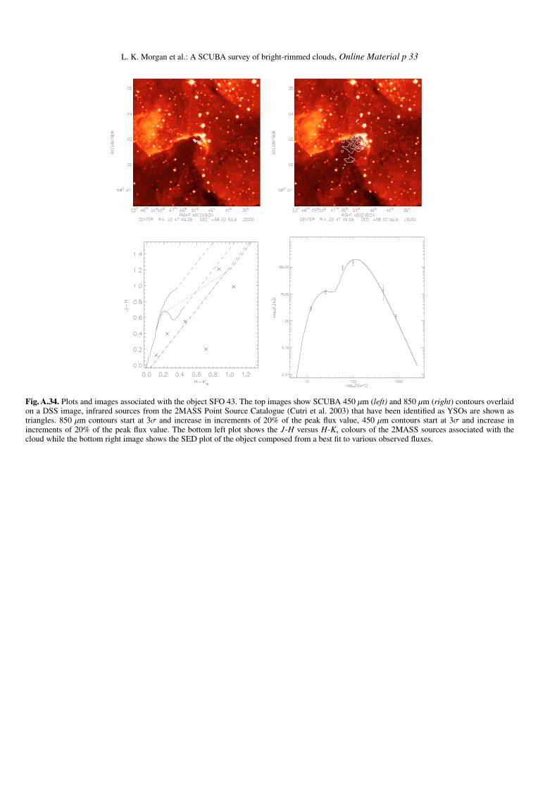
L. K. Morgan et al.: A SCUBA survey of bright-rimmed clouds, Online Material p 33
Fig. A.34. Plots and images associated with the object SFO 43. The top images show SCUBA 450 µm (left) and 850 µm (right) contours overlaidon a DSS image, infrared sources from the 2MASS Point Source Catalogue (Cutri et al. 2003) that have been identified as YSOs are shown astriangles. 850 µm contours start at 3σ and increase in increments of 20% of the peak flux value, 450 µm contours start at 3σ and increase inincrements of 20% of the peak flux value. The bottom left plot shows the J-H versus H-Ks colours of the 2MASS sources associated with thecloud while the bottom right image shows the SED plot of the object composed from a best fit to various observed fluxes.

L. K. Morgan et al.: A SCUBA survey of bright-rimmed clouds, Online Material p 34
Fig. A.35. Plots and images associated with the object SFO 44. The top images show SCUBA 450 µm (left) and 850 µm (right) contours overlaidon a DSS image, infrared sources from the 2MASS Point Source Catalogue (Cutri et al. 2003) that have been identified as YSOs are shown astriangles. 850 µm contours start at 6σ and increase in increments of 20% of the peak flux value, 450 µm contours start at 3σ and increase inincrements of 20% of the peak flux value. The bottom plot shows the J-H versus H-Ks colours of the 2MASS sources associated with the cloud.
Fig. A.36. Plots and images associated with the object SFO 45. The left image shows SCUBA 850 µm contours overlaid on a DSS image, infraredsources from the 2MASS Point Source Catalogue (Cutri et al. 2003) are shown as triangles. 850 µm contours start at 3σ and increase in incrementsof 20% of the peak flux value. The right plot shows the J-H versus H-Ks colours of the 2MASS sources associated with the cloud.

L. K. Morgan et al.: A SCUBA survey of bright-rimmed clouds, Online Material p 35
Fig. A.37. Plots and images associated with the object SFO 87a. The top images show SCUBA 450 µm (left) and 850 µm (right) contours overlaidon a DSS image, infrared sources from the 2MASS Point Source Catalogue (Cutri et al. 2003) that have been identified as YSOs are shown astriangles. 850 µm contours start at 7σ and increase in increments of 20% of the peak flux value, 450 µm contours start at 3σ and increase inincrements of 20% of the peak flux value. The bottom left plot shows the J-H versus H-Ks colours of the 2MASS sources associated with thecloud while the bottom right image shows the SED plot of the object composed from a best fit to various observed fluxes.

L. K. Morgan et al.: A SCUBA survey of bright-rimmed clouds, Online Material p 36
Fig. A.38. Plots and images associated with the object SFO 87b. The top images show SCUBA 450 µm (left) and 850 µm (right) contours overlaidon a DSS image, infrared sources from the 2MASS Point Source Catalogue (Cutri et al. 2003) that have been identified as YSOs are shown astriangles. 850 µm contours start at 4σ and increase in increments of 20% of the peak flux value, 450 µm contours start at 3σ and increase inincrements of 20% of the peak flux value. The bottom left plot shows the J-H versus H-Ks colours of the 2MASS sources associated with thecloud while the bottom right image shows the SED plot of the object composed from a best fit to various observed fluxes.

L. K. Morgan et al.: A SCUBA survey of bright-rimmed clouds, Online Material p 37
Fig. A.39. Plots and images associated with the object SFO 88. The top images show SCUBA 450 µm (left) and 850 µm (right) contours overlaidon a DSS image, infrared sources from the 2MASS Point Source Catalogue (Cutri et al. 2003) that have been identified as YSOs are shown astriangles. 850 µm contours start at 9σ and increase in increments of 20% of the peak flux value, 450 µm contours start at 4σ and increase inincrements of 20% of the peak flux value. The bottom plot shows the J-H versus H-Ks colours of the 2MASS sources associated with the cloud.

L. K. Morgan et al.: A SCUBA survey of bright-rimmed clouds, Online Material p 38
Fig. A.40. Plots and images associated with the object SFO 89. The top images show SCUBA 450 µm (left) and 850 µm (right) contours overlaidon a DSS image, infrared sources from the 2MASS Point Source Catalogue (Cutri et al. 2003) that have been identified as YSOs are shown astriangles. 850 µm contours start at 9σ and increase in increments of 20% of the peak flux value, 450 µm contours start at 4σ and increase inincrements of 20% of the peak flux value. The bottom left plot shows the J-H versus H-Ks colours of the 2MASS sources associated with thecloud while the bottom right image shows the SED plot of the object composed from a best fit to various observed fluxes.