MIDLANDS STATE UNIVERSITY

DEPARTMENT OF SURVEYING AND GEOMATICS

SVG209 FUNDAMENTAL PRINCIPLES OF GEODESY

LECTURE NOTES

SEPTEMBER 2012

COMPILED BY

DAVID NJIKE

1

INTRODUCTIONThe module is an introduction to the principles of Geodesy, it exposes the students to the main concepts and applications of Geodesy. Students have been dealing with plane surveys where the earth is considered to be a flat plane. In Geodesy we are now dealing with surveys that cover large areas where the curvature of the earth can longer be ignored. The main thrust of the module deals with geometrical Geodesy.

MODULE OBJECTIVESThe main objectives of the module are: 1. To introduce the students to the concepts of geometrical Geodesy. 2. To discuss the developments of Geodesy3. To introduce the geometry of the Ellipsoid 4. To explain geodetic coordinates5. To discuss transformations

MODULE OUTLINE1. Introduction

1.1. Introduction1.2. Definitions of Geodesy1.3. Concepts of Geodesy1.4. Geodesy and other Earth Sciences1.5. Branches of Geodesy1.6. Functions of Geodesy1.7. Observation techniques in Geodesy1.8. Applications of Geodesy1.9. Why should a Surveyor study Geodesy

2. Historical developments on Geodesy2.1. The Shape of the Earth2.2. Spherical Earth model2.3. Ellipsoidal Earth model2.4. Arc measurements2.5. The Geoid and Ellipsoid2.6. Dawn of the space age

3. Geometry of an Ellipsoid3.1. Geometry on the Sphere3.2. Construction of the ellipse3.3. Properties of an Ellipse3.4. Types of Latitude3.5. Coordinates of points in the Meridian3.6. Radii of curvature on the Ellipsoid3.7. Lines on the Ellipsoid3.8. Convergence

4. Ellipsoid Reference System4.1. Shape and Size of the Ellipsoid

2

4.2. Determining Global Best-fit Ellipsoids from Arcs of Meridians or Parallel4.3. Determining Global Best-fit Ellipsoids from Gravity Measurements4.4. Determining Global Best-fit Ellipsoids4.5. The Direction of the minor Axis

5. Relative positioning on the Ellipsoid5.1. Reduction of Observations5.2. Geodetic Problems

6. Coordinate Systems6.1. 2D coordinate systems6.2. 3D system6.3. Geodetic coordinate system6.4. Variations in coordinate systems

7. Coordinate transformations7.1. Transformation between coordinate systems7.2. Conversion between Ellipsoidal and Grid coordinates7.3. Conversion between Geographical and Cartesian coordinates7.4. Bursa-Wolf Model

LITERATURE Geodesy by G. Bomford Geodesy: The Concepts by Peter Vancek Control Surveys in Civil Engineering by MA Cooper Fundamentals of Geodesy by

3

1. INTRODUCTION

1.1. IntroductionGeodesy: is the oldest among the earth's sciences Dating back to the Summaritans 5000 years ago when man first become interested with

his surroundings. It all started with the concern of what is "my house's immediate vicinity" Latter it expanded to the distances of markets and exchange places. and with developments of transportation, man become interested in his "whole world".1.2. Definitions of Geodesy Geodesy came from the Greek words 'geo' ad 'desa' which means... "earth" and to

"divide". Webster defines Geodesy as:

'that branch of applied mathematics which determines by observations and measurement the exact positions of points and the figure and areas of large portions of the earth's surface, the size and shape of the earth, and the variations in the terrestrial gravity and magnetism '.

AGU Definition: "The science that determines the size and shape of the earth, the precise positions and elevations of points, and lengths and directions of lines on the earth's surface, and the variations of terrestrial gravity"

Classical definition of Geodesy is:'the science of measuring and portraying the earth's surface' (F. R. Helmert 1880)

Contemporary definition of Geodesy is:'the discipline that deals with the measurement and representation of the earth's surface, including its gravity field in three dimensional time varying space' (Vanicek and Krakiwsky 1986)

Other definitions:

'The branch of science that deals with the precise observations and measurement of the size and shape of the Earth, the mapping of points on its surface, and the study of its gravitational field'.

'A branch of applied mathematics which through precise observations and measurements determine the exact position of points, figures and areas and external gravity field of large portions of the earth's surface as well as the earth as a whole and variations of these with time'.

'The determination of the time varying size and figure of the earth by such direct measurements such as triangulation, levelling and gravimetric observations'.

1.3. Concepts of geodesyAll the concepts of Geodesy will include 3 general ideas or concepts: the size and shape of the earth the gravity field of the earth the positioning of the points on the surface of the earth.In its modern definition it also include measurement and modelling of the geodynamic phenomena such as polar motion, earth rotation and crustal deformation.

4

1.4. Geodesy and other earth sciences

1.5. Branches of Geodesy

5

MAPPING

G E

O D

E S

Y

MATHEMATICS

URBAN MANAGEMENT

BOUNDARY DERMACATION

GEOGRAPHY

ENVIRONMENTMANAGEMENT

ECOLOGY

PLANETOLOGY HYDROLOGY

PHYSICSCOMPUTER SCIENCE

ENGINEERINGPROJECTS

GEO

PHYS

ICS

SPAC

E SC

IEN

CE

OCE

ANO

LOGY

GEO

LOGY

ATM

OSP

HERI

C SC

I.

ASTR

ON

OM

Y

IRRI

GATI

ON

PR

OJE

CTS

Geometric Geodesy deals with the shape and size of earth, distance and direction of lines on earth, reference datums, and coordinate systems

Gravimetric or Physical Geodesy is the science that studies geophysical and geodynamic properties of earth, and includes earth gravity field and attractions of sun, moon and planets

Satellite Geodesy deals with the study of satellite orbits, motion, perturbations, and satellite based positioning

Geodetic Astronomy is a branch of geodesy which develops the theories and methods of constructing astronomical geodetic networks and defining the shape, dimensions, and gravitational field of the earth.

The term “astronomical geodesy” arose in the first half of the 20th century in Germany and is applied in the discussion of basic scientific problems concerning the geodesy of the earth as a planet as a whole on the basis of astronomical, geodetic and gravimetric measurements on the earth’s surface and in nearby space. In contemporary literature questions in astronomical geodesy are included in the branches of geodesy called theoretical geodesy and satellite geodesy.

1.6. Functions of Geodesy Establishing reference datums and coordinate systems for the definition of:• horizontal positions of points • distances and directions between points • elevations of points

Mathematical projections necessary to depict the datum surface on a map

6

GEODESY

PHYSICAL GEODESY

GEOMETRIC GEODESY

GEODETIC ASTRONOMY

SATELLITE GEODESY

Determination of geophysical properties such as the gravity field on or near the surface of the earth, geoid (mean sea level) and deflection of vertical (plumb line).

Study and monitor the geo-dynamics phenomena such as ocean and earth tides, crustal (tectonic) movements, polar motion, and the variations in earth rotation and gravity field.

1.7. Observation techniques in GeodesyThere are three basic observation techniques that are used in Geodesy, these are:

Astronomical Terrestrial Space

Astronomic Observations • Latitude, Longitude • Azimuth • Very Long Baseline Interferometry (VLBI) • Observations necessary to monitor polar motion, precession, nutation, etc.

Terrestrial Observations • Arc measurements (historic) • Triangulation, Trilateration, Traversing • Levelling • Zenith or vertical angles • Gravity

Space Based Observations • Lunar laser ranging • Satellite laser ranging • Satellite positioning • Satellite altimetry

1.8. Applications of Geodesy Surveying and mapping Defence Geophysical explorations Space explorations Communication, Navigation, etc.

Geodesy is the common link connecting • Surveying • Photogrammetry • Cartography • Geodynamics • Geophysics • Physics

1.9. Why should a Surveyor study Geodesy

7

Geodetic control surveys • Understanding geodetic datums and coordinate systems, e.g. NAD-83, WGS-84 • Difference between geodetic and astronomic coordinates • Different between geodetic and astronomic azimuth • Azimuth change due to convergence of meridians • Lengths of lines on the datum surface • Reduction of measured lines to datum surface

Geodetic levelling • Different datums (geoids), e.g. NGVD29, NAVD88 • Orthometric height and dynamic height • Effect of gravity on levelling

GNSS Surveys • Satellite datum(s) • GNSS derived coordinates and baselines • GNSS derived orthometric heights (elevations

State Plane Coordinates • Why is it needed? • Definition and implementation • Relevant computations

A knowledge of geodetic principles are needed in any survey that • Covers a very large area or a distance • Has to meet very high accuracy standards • Uses specialized techniques such as GNSS

8

2. HISTORICAL DEVELOPMENTS ON GEODESY

2.1. Introduction from earliest times man was increasing his knowledge of the planet he noticed the changing lengths of daylight changes in maximum height of the sun as the year progressed distant ships disappeared the lower parts first and the mast last Pole star changed altitude as one moved N-S direction and did not change as one moved

E-W direction at midday, length of shadow changed as one moved N-S and remained unchanged in E-W

direction

2.2. The shape of the EarthIt was the shape that came first:

It began with the Greeks (Homer) theorizing the earth as a 'flat' disc The Anaximander aka Anaximeues thought the earth as a rectangular object Next was the view of earth as a sphere but exactly when the notion of spherically

shaped earth first came into existence is not known However, recorded history reveals that as early as the 6th century BC a Greek

philosopher by the name Pythagorus believed earth was not flat but round 3 centuries later Aristotle (384-322 BC) considered the idea of a round earth as he

studied the movement of planets From his observations, particularly those of lunar eclipses, he concluded that the earth

was indeed spherical in shape

2.3. The size of the EarthAfter the shape, the size came in:

The first approximation of the earth's circumference was proposed by Plato at 40000 miles

Meanwhile around 250 BC in Egypt, a Greek scholar and philosopher, Eratosthenes set out for a more explicit measurement of the size of the earth

Eratosthenes developed a simple method for calculating earth's circumference Using a knowledge of the sun's position relative to the earth and some principle of

geometry, he calculated the earth's equatorial circumference to be 25000 miles the search for a better figure that defines the shape of the earth continues In the 7th century the theory that the earth is not a perfect sphere arises However these resulted to an intense controversy between the French and the English The English claimed that the earth must be flattened but the French defended their

claim for an egg-shaped earth

2.4. Spherical Earth ModelErastothenes (276 - 195 BC) of Alexander, made the first measurement of the radius of the earth using the principle of arc measurement

9

Willebrord Snelius (1550 - 1626) conducted the first triangulation (33 triangles) in 1615 in Holland covering a latitude of 10 11' or about 120km.

Newton in about 1666 conceived the law of universal gravitaion and his laws of motion and from purely dynamical consideartions proposed that the earth approximated an oblate spheroid very closely.

Through the initiative of the French Academy of Sceinces founded in 1666, France became the leader in Geodesy in the 17th and 18th centuries. The Abbe J. Picard in 1670 carried out an arc measurement trough Paris with the aid of a triangulation network and was the first to use a telescope with cross hairs. His value for the radius of the earth was in error by 0.01% and aided Newton in the verification of his law of gravitation.

However, the outcome of 31 years of effort spent on the arc of meridian through Paris indicated that the polar axis of the earth was longer than the equatorial one, in other words, that the earth was prolate and therefore at variance with Newton's concept.

2.5. Ellipsoidal Earth ModelIn order to resolve the issue, the French Academy sent two expeditions, one to Peru (1735) near the equator and the other to Lalpand (1736) north of the Arctic Circle. The purpose of the expeditions was to determine the length of a degree of Latitude in each of the two countries.

The results of the measurement in Lapland by Clairaut and others confirmed polar flattening and the comparisons of this arc with that in Peru (which took 10 years) put the matter beyond doubt and led to a better determination of the flattening (f = a-b/a = 1/120). The flattening of the earth at the poles was thus demonstrated by geodetic measurements.

However, Clairaut (1713 - 17650) developed the theorem in 1743 named after him, which permits the computation of the flattening from two gravity measurements at different latitudes. The practical application of this grvametric method suffered until the 20th century from the paucity of accurate and well-distributed gravity measurements and from the problem of reducing these to the ellipsoid. 2.6. Arc MeasurementsAfter the rotational ellipsoid had asserted itself as a model for the figure of the earth many arc measurements using triangulation were made until the mid-19th century. These include both measurements along a meridian and also along a parallel.

Many arc measurements were carried out in the 19th and 20th centuries, which were largely the bases for geodetic surveys. Of the older arcs, two of the most important were that due to Gauss (between Gottingen and Altona, 1821 - 1825, adjusted by least squares) and also Bessel and Baeyer (arc measurement oblique to the meridian in East Prussia, 1831 - 1838).

10

More recent long arc measurements are:1. American meridian arc (Alaska - Terra del Fuego)2. West European - African meridian arc along meridian of Paris (Shetland - Algeria)3. Arctic Ocean-Mediterranean sea meridian arc (Hammerfest - Creto).4. African meridian arc tied to it at 300 east (Cairo - cape Town).5. European-Asiatic longitude arc measurement at 480 latitude (Brest - Astrakhan) and at 520

(Ireland - Ural Mountains)6. Indian latitude and longitude arc measurements

The African triangulation chain along the 30th arc of meridian was completed in 1954, when the remaining gaps in Uganda/Kenya and Ethiopia were closed. This provided an unbroken arc of 1000 of latitude extending from port Elizabeth in South Africa to North Russia.

National networks of triangulation started to appear from the mid-18th century, Bavaria (1764), England (1783), India (1802), Russia (1817) and the USA (1846) to mention a few. The primary triangulation of Zimbabwe was started in 1901 and completed in 1973. 2.7. The Geoid and EllipsoidFrom the early 19th century men such as Laplace CF Gauss and F. W. Bessel recognised the need to take into account the deviation of the geoid surface from the ellipsoid, which gives rise to what is known as the deflection of the vertical (plumb line from ellipsoid normal). All measurements refer to the plumb line and not the ellipsoidal normal. F. R. Helmert (1843 - 1917) made the transition to the current concept of the figure of the earth, whereby the deflections of the vertical are taken into account in the computation of the ellipsoidal parameters, a, f.

mainly due to the efforts of individuals geodesists as many as 18 ellipsoids of reference had been calculated by 1939. Of these Hayford's 1909 figure was the first to be determined from more than only arc data - plumb line deviations being incorporated in the calculations as well. in 1924 Hayford's figure was accepted by the IUGG as the International Ellipsoid. Six years later, Cassini's formula for normal gravity, based on Hayford's reference figure and Clairaut's theory was adopted by the IUGG as the International Gravity Formula. Thus 200 years after Clairaut had proved Newton's oblate earth hypothesis to be correct and almost 2000years after Eratosthenes spherical earth result the earth model became a rotating biaxial ellipsoid with a modelling surface gravity.

Completion of the great arcs spanning the major continents in 1054 made possible a better determination of the earth model. Two determinations were carried out soon afterwards in the United states of America, the first by Hough in 1956 and the next year by Fischer and Chovitz. This was all in preparation for the putting into orbit of the first American artificial earth satellite. When Hough's ellipsoid was used for satellite tracking purposes it was found that the flattening constant that bad been introduced into the calculations was too inaccurate for orbit prediction purposes.

11

2.8. Dawn of the Space AgeThe first satellites put into orbit by the Americans and British indicated a flattening of the earth closer to one in 298 rather than one in 297 as determined up to that time. this means that the polar diameter of the earth is about 43km shorter than the equatorial diameter of 12756 km and therefore the earth shape departs only marginally from that of a sphere. However the difference is still too great for the purposes of geodesy and precise navigation.

Early applications of close orbit satellites in geodesy for point determination treated the satellite purely as a moving beacon which could be observed photographically. The accurate space direction to the satellite was obtained relative to the precisely known positions of the stars whose images appeared on the photo plate.

In 1966 NASA in conjunction with the US DoD and NGS launched a World Net Geodetic Project which was the most extensive geodetic survey ever undertaken by man, and which involved 45 ground stations at average distances apart 0f 2400 km and the PAGEOS light reflecting satellite. An overall coordinate accuracy of 45 metres was obtained for the 45 stations 3-D geocentric coordinates.

Following the launching of the Russian satellite Sputnik 1, two scientists of the John Hopkins University conducted experiments to determine this satellite's orbit by measuring the Doppler shift of its radio signals. The so-called Navy Navigation Satellite System (NNSS) or the Transit or NAVSAT System evolved from this work. NNSS became operational in 1964 for Polaris submarines but was classified as secret until 1967 where after it was released for general world-wide use. Between 1967 and 1973 six Transit satellites were placed in orbit to serve NAVSAT. Each weighs 135 pounds and was launched to a height of approximately 1100km above the earth by a small military rocket. They circle the earth every 107 minutes in circular polar orbits forming a cage within which the earth rotates and transmit two very stable frequencies of 150 and 400 MHz timing marks and a navigational message describing the satellite's position in terms of time. By receiving these signals during a single pass above the horizon and measuring the amount by which the received signal frequency changes as the satellite approaches or recedes, a user can obtain his position accurately.

The US DoD has complicated the introduction of a new system called NAVSTAR or Global Positioning System (GPS) to replace NAVSAT. NAVSTAR comprises 18 satellites each at altitudes of roughly 20200 km above the earth orbiting in three planes with six satellites per plane. The orbits are determined relative to a geocentric reference system called the DoD World Geodetic System (WGS 1984) and there are always at least four satellites above the horizon available for position fixing. The relative positions of ground stations hundreds of kilometres apart can now be determined to accuracies of more than 1 ppm.

Another development of great geodetic significance is what is known as Very Long Baseline Interferometry (VLBI). This involves two astronomical radio antennae separated by several thousand kilometres which simultaneously receive radio emissions from quasers or very distant extra-galactic near-point sources of radio energy. The length of the interferometer

12

baseline obtained is obtained from the difference between the arrival times of the quaser signal at each antenna and the speed of light in vacuo, which is known very accurately. The error in distance only amounts to a few centimetres and thus is small enough to detect the movement between tectonic plates. The technique is being used to establish a world-wide 3-D geodetic net to a far higher accuracy than was possible before.

Other satellite techniques include satellite altimetry which uses radar pulses to measure the perpendicular distance between the satellite and the surface of the ocean. The data can be analysed for a determination of sea surface topography and the geoid as well as details of the gravity field.

Laser technology has made possible laser distance measurement (SLR) to satellites equipped with reflectors and also to the moon where laser reflectors were deposited by the Apollo missions from 1969 onwards. Assignment 1: Give a detailed account of how the following contributed to the history and development of Geodesy:

Pythagoras Aristotle Archimedes Eratosthenes Poseidonius I-Hsing Al-Mamum Columbus Frisius and Snellius Fernel Picard The Cassinis Mason and Dixon Newton Johann Carl Friedrich Gauss John Harrison Helmert Ferdinard Hassler

13

3. GEOMETRY OF AN ELLIPSOID3.1. The Shape of the Earth The earth is covered with two types of material

o Land masseso Water bodies (seas, oceans)

The land mass is highly irregular Water bodies are regular surfaces 70% of the earth is covered by water bodies The 'sea level' can be used to describe the earth Average level of the sea water is called Mean Sea LevelThe Geoid If the land masses were covered by a network of canals through which the waters of

the oceans were permitted to flow freely (frictionless) under gravity, neglecting tidal effects, the surface of water on the canals and the oceans would form an equipotential surface called the geoid, which simply means "Earth shaped".

The geoid is that equipotential surface (no work done moving on the surface) that approximate the MSL in a least square sense.

At any point on the geoid, the direction of gravity is perpendicular to the geoid The earth's structure is not homogenous and its variations causes the gravity to change The geoid is a smooth surface but is undulatory The geoid is a physical, solid surface It does not have a mathematical representation It is not a fully known surface because of the sparseness of gravity observations over

large areas of the earth particularly the oceans It does not have a mathematical representationThe Ellipsoid The simplest mathematically regular surface which fits the geoid is an oblate spheroid. As a result of various measurements carried out since the 18th century in different parts of the world, a number of geodesists have produced estimates of the size of spheroid which best fits the geoid for the part of the earth considered in the calculations i.e. various countries or parts of the world have adopted localised spheroids which closely conforms to the geoid at that particular place in question and whose radius equals the radius of curvature of the spheroid at that point. Such an approximation treatment enables one to calculate the results of surveys covering large areas of more than 30km.Ellipsoid is a mathematical surfaceSpheroid and EllipsoidSpheroid - solid generated by rotating an ellipse about either axis

Oblate spheroid - rotated about minor axisProlate spheroid - rotated about its major axis

Ellipsoid - solid for which all plane sections through one axis are ellipses and through the other ellipses or circles

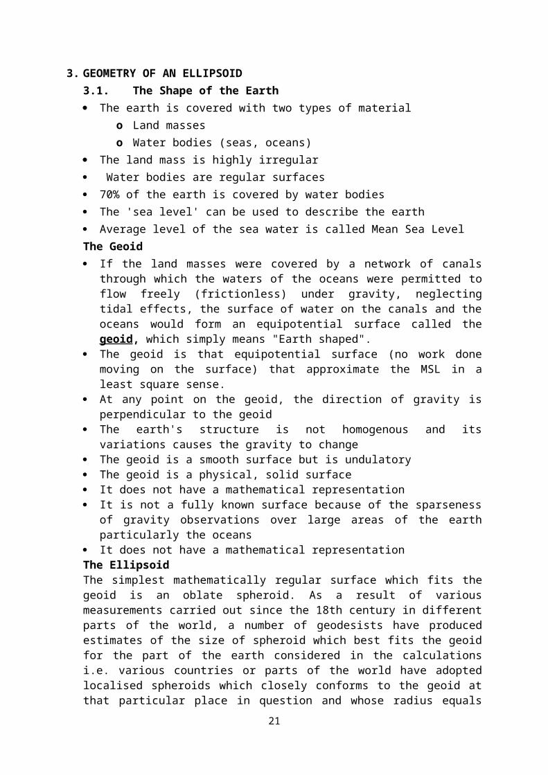
3.2. The Sphere a) Great circlesb) Small circlesc) North Pole and South Poled) Longitude

14

e) Meridianf) Latitudeg) Equator

The circle containing CDE is a great circle; that containing AB is a small circle.

15

16

17

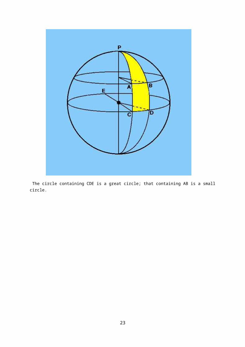
refer to geometry on the sphere handout (pdf) (Appendix 1)

3.3. The EllipsoidAn ellipsoid is obtained by rotating an ellipse about its minor axis. The minor axis coincides with the earth's spin axis, the major axis sweeps out an equatorial plane as the ellipse is rotated. Any cross section of the ellipsoid containing both poles is a meridian section and shows the form of the original ellipse. 3.4. Construction of an EllipseThere are three ways to construct an ellipse:

mechanical method graphical method computation method

Mechanical method use a piece of string and a pencil anchor the string ends down on the paper, a few cm apart take up the slack with the pencil and trace out an ellipse while keeping the string taut the other half is drawn by taking up the slack in the opposite direction

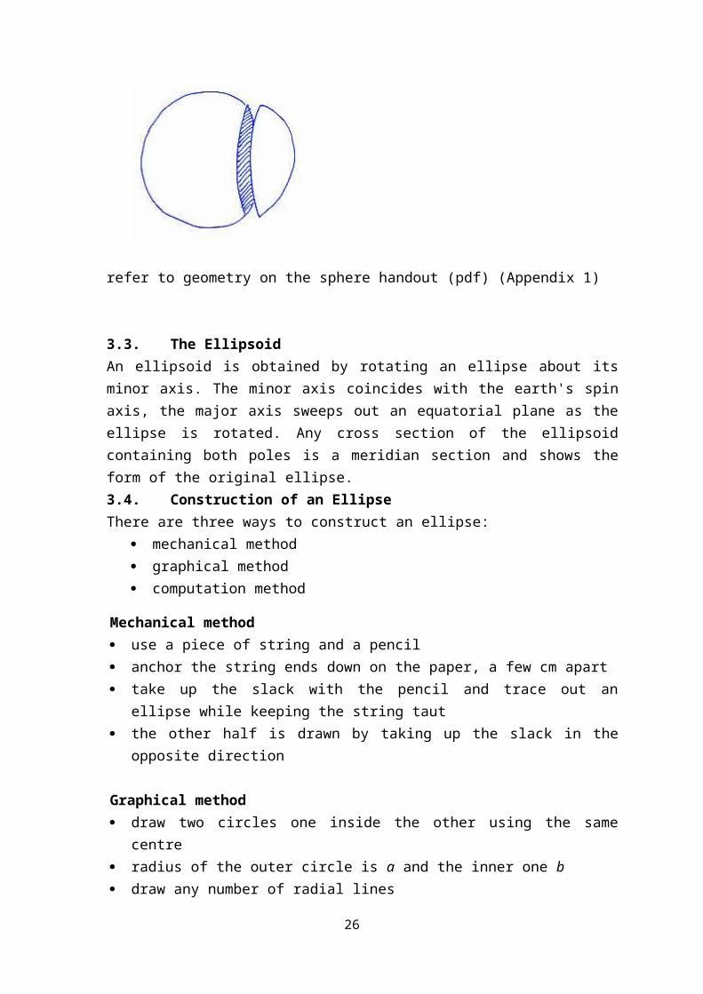
Graphical method draw two circles one inside the other using the same centre radius of the outer circle is a and the inner one b draw any number of radial lines draw horizontal line from the intersection of the radial line and the inner circle draw vertical lines from the intersection of radial line with the outer circle mark the intersections of the two line from the same radial line connect the points which form the ellipse

18

Computations most efficient way compute X and Z coordinates for a sufficient number or points and plot them directly

X = acos∅

(1−e2 sin2∅ )12

Z = a(1−e2)sin∅

(1−e2 sin2∅)12

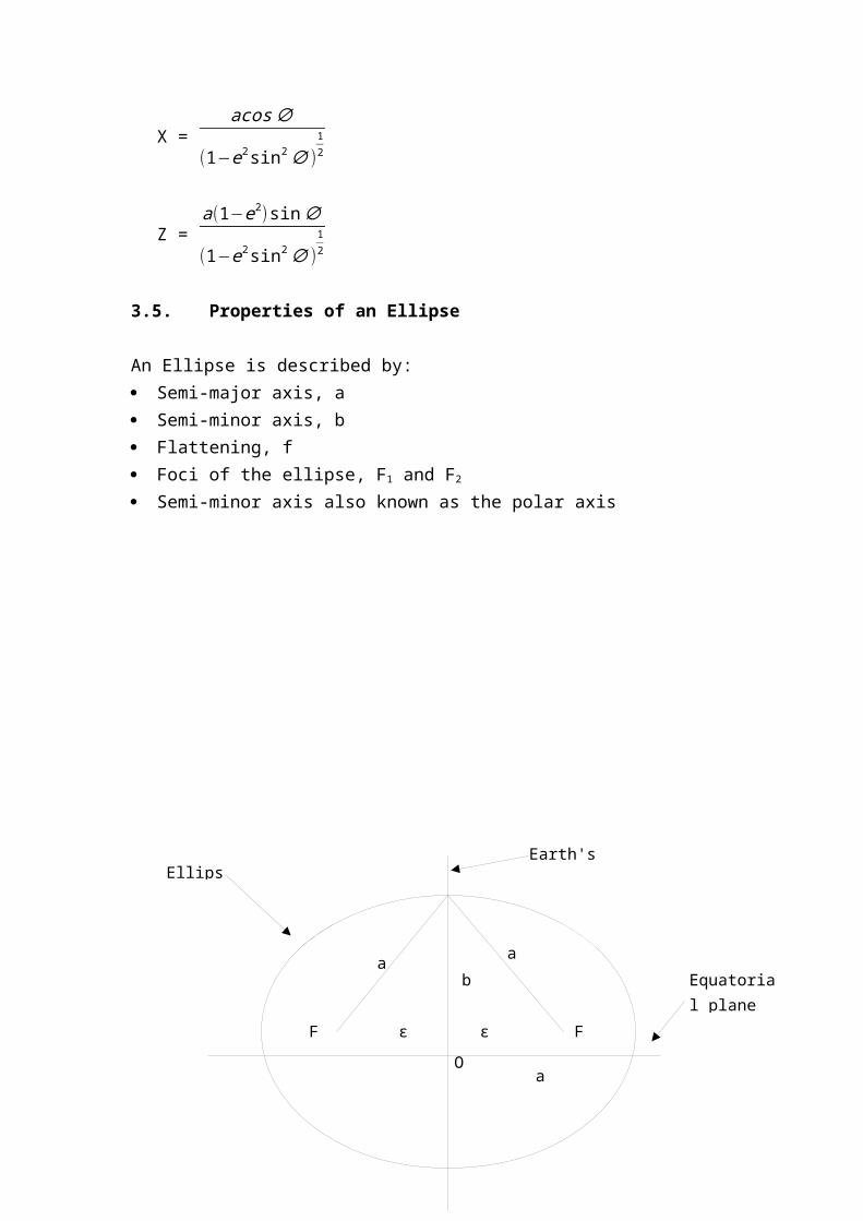
3.5. Properties of an Ellipse

An Ellipse is described by: Semi-major axis, a Semi-minor axis, b Flattening, f Foci of the ellipse, F1 and F2

Semi-minor axis also known as the polar axis

19

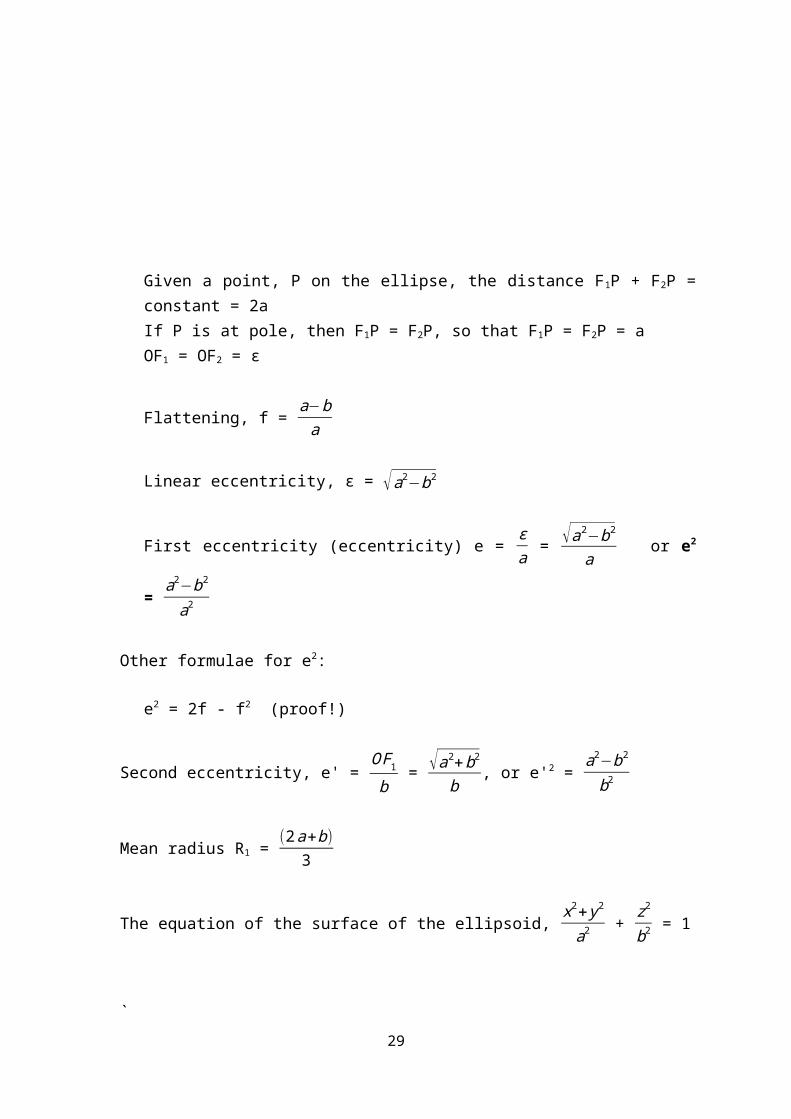
Given a point, P on the ellipse, the distance F1P + F2P = constant = 2aIf P is at pole, then F1P = F2P, so that F1P = F2P = aOF1 = OF2 = ε

Flattening, f = a−b

a

Linear eccentricity, ε = √a2−b2

First eccentricity (eccentricity) e = εa = √a2−b2

a or e2 = a

2−b2

a2

Other formulae for e2:

e2 = 2f - f2 (proof!)

Second eccentricity, e' = O F1

b = √a2+b2

b, or e'2 = a2−b2

b2

Mean radius R1 = (2a+b)

3

20

O

Earth's polar axis

Equatorial plane

a

b

εε F2F1

a a

Ellipse

i E

M

M’

ψ φ

β

b

a

Z

X

p

The equation of the surface of the ellipsoid, x2+ y2

a2 + z2

b2 = 1

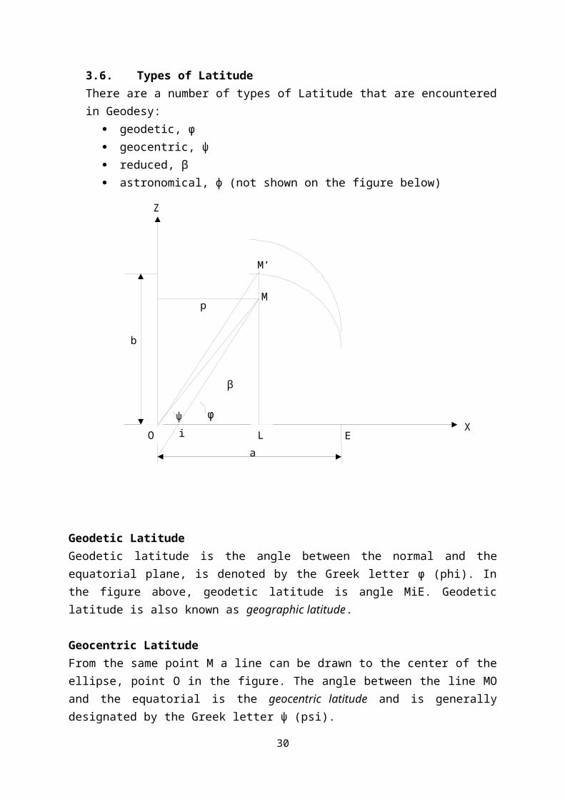
`3.6. Types of LatitudeThere are a number of types of Latitude that are encountered in Geodesy:

geodetic, φ geocentric, ψ reduced, β astronomical, ɸ (not shown on the figure below)

Geodetic LatitudeGeodetic latitude is the angle between the normal and the equatorial plane, is denoted by the Greek letter φ (phi). In the figure above, geodetic latitude is angle MiE. Geodetic latitude is also known as geographic latitude.

Geocentric LatitudeFrom the same point M a line can be drawn to the center of the ellipse, point O in the figure. The angle between the line MO and the equatorial is the geocentric latitude and is generally designated by the Greek letter ψ (psi).

Reduced Latitude

21

LO

Through the same point M assume a point is projected in a direction parallel to the polar axis until it intersects a circle of radius a at point M’. The angle between the radius M’O and the equatorial plane is known as the reduced latitude or eccentric angle, and is generally designated by the Greek letter β (beta).

Astronomical latitudeAstronomical latitude is the angle formed by the direction of gravity (the plumb line) and the equatorial plane. The astronomical latitude is often designated by the capital Greek letter ɸ (PHI).

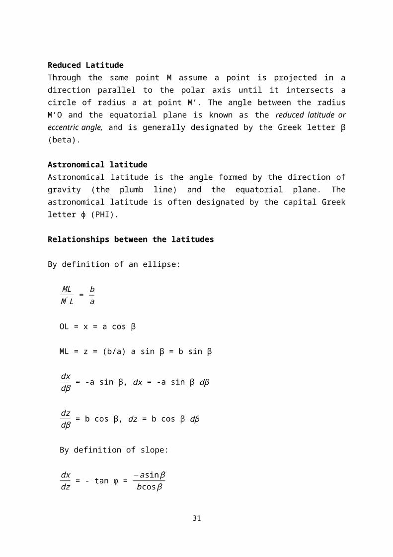
Relationships between the latitudes

By definition of an ellipse:

MLM ' L

= ba

OL = x = a cos β

ML = z = (b/a) a sin β = b sin β

dxdβ = -a sin β, dx = -a sin β dβ

dzdβ = b cos β, dz = b cos β dβ

By definition of slope:

dxdz = - tan φ =

−a sin βb cos β

tan φ = ab tan β

tan ψ = zx =

b sin βa cos β =

ba tan β

= ba ( b

atanφ ) = b

2

a2 tan φ

= (1 – e2) tan φ

Other relationships among these latitudes are as follows:

22

φ+90

Z

P

φ

x

z

Z

X

tan ψ = (1 – e2) tan φ = b2

a2 tan φ

tan ψ = (1 – e2)1/2 tan β = ba tan β

tan β = (1 – e2)1/2 tan φ = ba tan φ

tan β = tanψ

(1−e2 )1 /2 = ab

tan ψ

tan φ = tanψ

(1−e2 )1 /2 = a2

b2 tanψ

tan φ = tan β

(1−e2 )1 /2 = ab

tan β

3.6. Coordinates of points in the Meridian

For an ellipse in a point G’s meridian plane (note: x is p in the previous figure)

23

x2

b2 + z2

b2 = 1

z = [(1− x2

a2 )b2]1/2 = ba (a2 – x2)1/2

The slope of a point is given by the first derivative, or:

dzdx =

b2 a ( 1

a2−x2 )1/2(-2x) = - ba

x√a2−x2

But (a2 – x2)1/2 = ab

z so dzdx = - b

2 xa2 z

From geometry dzdx = - cot φ

Substituting cot φ = b2 xa2 z

or tan φ = a2 zb2 x

Since e2 = 1 - b2

a2 then tan φ = z

x(1−e2) so

zx = (1 – e2) tan φ

From x2

b2 + z2

b2 = 1, we have x2 + a2

b2 z2 = a2

Substituting b2 = a2(1 – e2), we have x2 + ( z2

1−e2 ) = a2 so (a2 – x2)(1 – e2) = z2

Equating the above equations (a2 – x2)(1 – e2) = x2(1 – e2)2 tan2 φ or a2 = x2 + x2(1 – e2)2 tan2 φ = x2 [1 + (1 – e2)2 tan2 φ] = x2(1 + tan2φ – e2 tan2φ)

Since sec2φ = 1 + tan2φ then a2 = x2(sec2 φ−e2 si n2 φco s2 φ )

So a2 = x2

co s2 φ (1 – e2sin2φ) and thus x2 =

a2 co s2 φ(1−e2 si n2 φ )

Finally,

24

x2 = a cosφ

√(1−e2 si n2φ ) …………………………………………………..(1)

For z, z2 = (a2 – x2)(1 – e2) so substituting in for x, we get

z2 = a2 ( 1−e2 si n2 φ−cos2 φ1−e2 si n2 φ )(1 – e2)

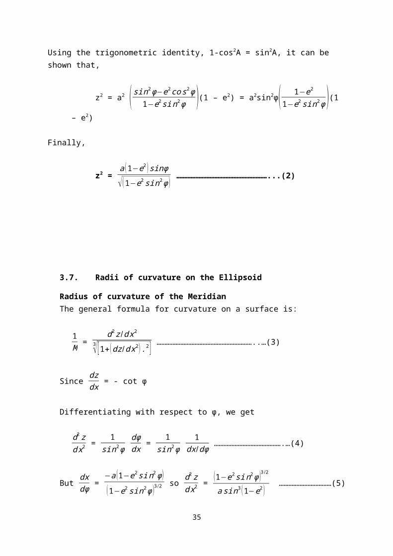
Using the trigonometric identity, 1-cos2A = sin2A, it can be shown that,

z2 = a2 ( si n2 φ−e2co s2 φ1−e2 si n2 φ )(1 – e2) = a2sin2φ( 1−e2

1−e2 si n2 φ )(1 – e2)

Finally,

z2 = a (1−e2) sinφ

√(1−e2 si n2φ ) …………………………………………………...(2)

3.7. Radii of curvature on the Ellipsoid

Radius of curvature of the MeridianThe general formula for curvature on a surface is:

1M =

d2 z /d x2

3√[1+( dz /d x2 ) .2 ] ……………………………………………………..…(3)

Since dzdx = - cot φ

Differentiating with respect to φ, we get

d2 zd x2 =

1si n2 φ

dφdx =

1si n2 φ

1

dx /dφ …………………………………….…(4)

But dxdφ =

−a (1−e2 si n2 φ )(1−e2 si n2 φ )3 /2 so d2 z

d x2 = (1−e2 si n2 φ )3 /2

a si n3 (1−e2) ……………………………(5)

25

x

N

Substituting (5) into (3) and dropping the minus sign by convention, we get

M = a (1−e2)

(1−e2 si n2 φ )3 /2 …………………..…………………….(6)

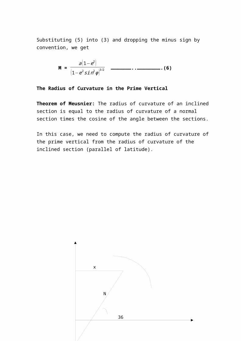
The Radius of Curvature in the Prime Vertical

Theorem of Meusnier: The radius of curvature of an inclined section is equal to the radius of curvature of a normal section times the cosine of the angle between the sections.

In this case, we need to compute the radius of curvature of the prime vertical from the radius of curvature of the inclined section (parallel of latitude).

26

From the figure above, the radius of the parallel of latitude = N cos φ = x coordinate in the meridian plane, and the angle between the inclined plane (parallel of latitude) and the

prime vertical is φ. Thus, N cos φ = a cosφ

(1−e2 si n2 φ )1 /2 or

N = a

(1−e2 si n2 φ )1 /2 ………………………………………………………….(7)

The Radius of Curvature at any Azimuth

Euler’s Formula for Curvature in an Arbitrary Direction:

1R = co s2 z

R1 + si n2 z

R2

Where R is the radius of curvature in an arbitrary direction, z in the angle from the principal section with the largest radius of curvature, R1, in a principal normal direction, and R2 is the radius curvature of the other normal direction.

In our case, R1 is the radius of curvature in the prime meridian, M. The angle z is the azimuth to the line and R2 is the radius of section perpendicular to the prime meridian which is N. Substituting in the appropriate equations we get:

1R = co s2 z

M + si n2 z

N

Thus R is:

R = MN

Nco s2 z+Msi n2 z ………………………………………………….(8)

Mean Radius of the Earth as a Sphere

The Gaussian mean radius is defined to be the integral mean value of R taken over the azimuth varying from 00 to 3600, or

R = 12 π∫0

2 π MNNco s2 z+Msi n2 z

dz

= √ MN

= a√ (1−e2 )1−e2 si n2 φ

27

Computation of Arc Lengths

Length of a Meridian Arc: G = ∫φ1

φ2

M dφ. This integral must be computed using

numerical methods.

Length of an arc of the circle of latitude: ∆ L = ∫λ 1

λ 2

Ncosφ dφ = N cosφ (λ2 – λ1)

where (λ2 – λ1) is in radians.

3.8. Lines on the EllipsoidBetween points P1and P2 on an ellipsoid, there can be infinite number of lines. Three are of interest in geodesy; the cord, the normal and the geodesic.

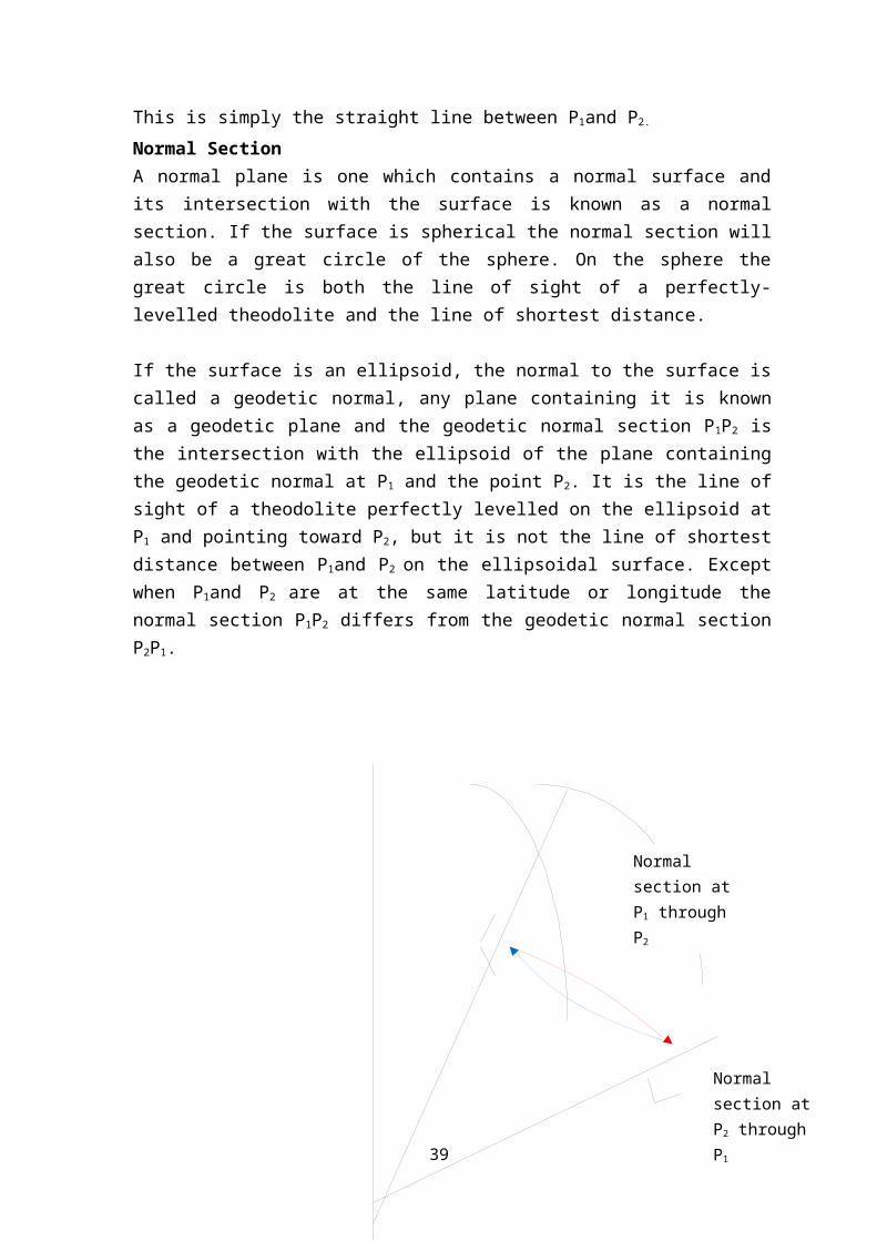
ChordThis is simply the straight line between P1and P2.

Normal SectionA normal plane is one which contains a normal surface and its intersection with the surface is known as a normal section. If the surface is spherical the normal section will also be a great circle of the sphere. On the sphere the great circle is both the line of sight of a perfectly-levelled theodolite and the line of shortest distance.

If the surface is an ellipsoid, the normal to the surface is called a geodetic normal, any plane containing it is known as a geodetic plane and the geodetic normal section P 1P2 is the intersection with the ellipsoid of the plane containing the geodetic normal at P1 and the point P2. It is the line of sight of a theodolite perfectly levelled on the ellipsoid at P1

and pointing toward P2, but it is not the line of shortest distance between P1and P2 on the ellipsoidal surface. Except when P1and P2 are at the same latitude or longitude the normal section P1P2 differs from the geodetic normal section P2P1.

28

Normal section at P1 through P2

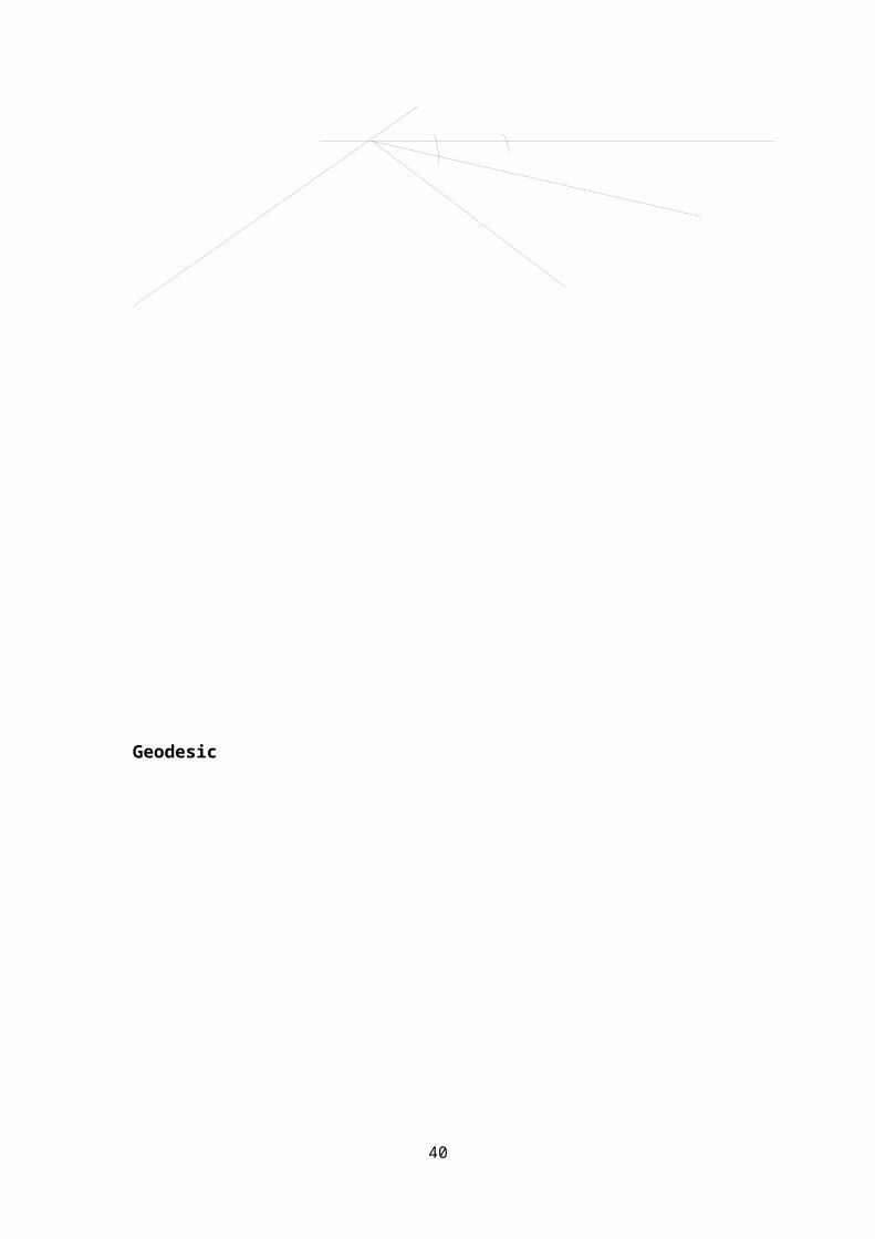
Geodesic

29

Normal section at P2 through P1

In a figure consisting of three points one can recognise six normal section azimuths, thus the use of normal sections introduces an ambiguity in the definition of an ellipsoidal triangle. The solution to this problem is provided by the geodesic curve, which is the curve which has the shortest length between two points on the ellipsoid. The azimuth of the geodesic is called the ellipsoidal azimuth (αE).

On any surface, the line of shortest distance between two points is known as the geodesic. On the sphere the great circle is the geodesic. On the ellipsoid the geodesic is usually a curve of double curvature which subdivides the angle between the two normal sections in the ratio 2:1. The difference between the normal section and geodesic azimuths is defined in the equation below. 3.9. Convergence

The reverse azimuth A21 will différ from the direct azimuth A12 by an amount which is usually not negligible. This quantity is termed convergence (ΔA) or sometimes meridian convergence, because its occurrence is due to the convergence of the meridians at points P1and P2 towards the pole. The following formula which is exact for a sphere can also be applied to each ellipsoids where the two points are less than 200 km apart.

ΔA = Δλ sinφm

Where φm = (φ1 + φ2)/2 and A21 = A12 + ΔA + 1800

30

4. ELLIPSOID REFERENCE SYSTEM

4.1. Definition of an Ellipsoidal Reference SystemThe following eight constants must be specified to define an ellipsoid reference system:

1. the size and shape of the ellipsoid (2 constants)2. the direction of the minor axis (2 constants)3. the position of the centre (3 constants)4. the zero of the longitude (1 constant)

4.2. Size and Shape of the EllipsoidTwo constants must be specified to define the size and shape of the ellipsoid, usually a and f, or a and e, or a and b. The choice of the ellipsoid is not very important - for small areas it makes virtually no difference which ellipsoid is used. Historically, countries have chosen ellipsoids for reasons such as:

a) Their choice was the best known ellipsoid for the whole earth at that time.b) It fits the geoid in their region particularly well.c) Neighbouring countries have chosen it

The IAG is continually collecting data regarding the best fit ellipsoid for the earth and regularly publishes its latest recommended values. Once a country has chosen on ellipsoid in practice however it is unlikely ever to change it although in Zimbabwe we are planning to move away from Modified Clarke 1880 onto WGS84.

There are a number of practical methods available for the determination of a best-fitting ellipsoid for the whole earth.

4.3. Determining Global best-fit Ellipsoids from Arcs of Meridian or ParallelsThe astronomical latitudes φp and φq at two point P and Q approximately on the same meridian are measured and a triangulation network connects P and Q. The network is approximately computed on any arbitrary ellipsoid to give geodetic coordinates for P and Q. The meridian distance PQ' is then computed from s and α, the computed distance and azimuth between P and Q.

We put φm = (φp + φp)/2 and Δφ = φp - φp

Then the radius of curvature in the meridian = PQ'/ Δφ i.e. a(1 - e2)/(1 - e2sin2φm)3/2 = PQ'/ Δφ

So we have one equation in terms of two unknowns a and e. Similar measurements at other latitudes will provide more equations, and after linearization we can obtain a least squares solution for a and e. To give values of a and e representative of the whole earth a large number of arcs, evenly distributed over the whole surface of the earth are required.

31

Any triangulation network of about a few hundred km north-south extant can be used as long as the necessary astronomical observations have been made.

The method is the classical geodetic way of determining the mean earth ellipsoid since the 17th century and many today's best known ellipsoids (e.g. Clarke, Everest, Airy, etc.) were computed in this way. If we have a predominantly east-west triangulation nework, we can use the method of arcs of parallel in which we measure longitude at two points P and Q almost on the same arc of parallel. We have:

acosφp/(1 - e2sin2φm)3/2 = PQ'/ Δλ

where, PQ' is the distance P and Q projected along the parallel through P and Δλ = λp -λq

This method has not been used as much as meridian arcs because of the difficulties of measuring accurate longitude differences before the advent of radio time signals.

Either method would give an anomalous result near large topographic an density anomalies owing to the deviation of the vertical. Both methods are essentially finding the ellipsoid which makes deviation of the vertical as small as possible on average because the basic equation assumes the normal and the vertical to be the same.

4.4. Determining Global best-fit Ellipsoids from Gravity MeasurementsThe simplest way to use observed gravity to determine the mean ellipsoid is to use Clairaut's formula for the gravitational attraction of a rotating ellipsoid. This formula gives the gravity γφ, at a latitude φ in terms of the gravity at the equator, γε

γφ = γε(1 + B2sin2φ)

where B2 is a function of the rate of rotation and flattening. If we have a large number of gravity observations on the earth's surface and reduce them to the geoid level, we will have a large number of pairs of values of γφ and φ which can be used to in Clairaut's formula and a least squares solution made for γε and B2. B2 can then be used with the known rate of rotation of the earth to give the flattening. A purely gravitational method such as this will give the shape of the earth but not its size.

This method is not used today as it is very crude. We are more likely to compute gravity anomalies at all points and use a more complex geopotential model. The latest solutions use the spherical harmonic model and a large number of harmonic coefficients are solved including the flattening.

Because gravity data is still so sparse, especially over the oceans, gravity actually gives a better indication of local variations in the geoid rather the earth's overall shape. But it is possible to continue gravity and meridian arc measurements and this was done in the determination of some of the ellipsoids (e.g Hayford) early this century.

32

4.5. Determining Global Best-fit EllipsoidsMost modern mean earth ellipsoids are based largely on observations to artificial earth satellites. Some of the methods used are:

1. by determining the Cartesian coordinates of a large number of stations on the earth's surface, reducing them to the geoid and fitting an ellipsoid in a geometrical way;

2. by measuring perturbations of satellite orbits and computing spherical harmonic coefficients;

3. by using satellite altimetry to give the sea surface directly, and thus the geoid over the oceans.

Nowadays, internationally recommended ellipsoids are produced from a combination of satellite, triangulation and gravity observations.

4.6. The Direction of the Minor AxisIn practice the minor axis is always made parallel to the mean axis of the earth (CTP). This parallelism is achieved by imposing the relationships inherent in the Laplace equation. A major advantage of this is that the minor axes of all ellipsoidal reference systems will be parallel to each other as long as they all use Greenwhich as the zero of longitude, then the transformation from one system to another in one merely of translation.

33

5. RELATIVE POSITIONING ON THE ELLIPSOID

5.1. Reduction of ObservationsThere are three kinds of observables used in relative horizontal positioning:

astronomical azimuth (A) direction (d) spatial distance (Δr)

If done properly the computation of horizontal positions using either a 3-D or 2-D approach, must yield identical results. When computing in 3-D the observations are not corrected other than for instrumental effects and refraction, because the computations are carried out in the same space as observations. Before horizontal positions in 2-D spaces are computed however it is necessary to apply corrections to the measurements. When computing on the reference ellipsoid measurements made on the earth's surface must be reduced to this ellipsoid first. Reduction of observations to computational surfaces is an integral part of the direct problem of position determination whilst after the solution of the inverse problem on the ellipsoid the derived quantities such as distance and azimuth need to be converted back to the terrain using the corrections in a negative sense.

In the reduction of observations onto the ellipsoid there are two groups of effects to be considered; geometrical effects, which arise as a result of the geometry of a biaxial ellipsoid and the effects of the gravity field, because geodetic instruments are aligned to the local plumb line and computations are carried out in a geometrical space.

Let us look first at the effect of gravity field on the observed astronomical azimuth A, because in most instances the directions of the plumb line and ellipsoidal normal do not coincide there will be a small difference between the astronomical and geodetic azimuths, known as the Laplace correction Δα = α -A or correction for the deflection for the deflection of the vertical, defined by the Laplace equation:

Δαij = -ηitanφ - (εisinαij - ηicosαij)cotZij = C1 + C2

If the deflection is zero, the correction is also equal to zero and for horizontal lines (Z = 900), the second term is zero as well. The geodetic azimuth obtained in this way is often called the Laplace azimuth.

34

Effect of skew normal

The next correction to be applied is the skew-normal correction which arises from the fact that the two ellipsoidal normals at Pi and Pj are skewed and not coplanar. The azimuth α’ij

(normal section azimuth) on the ellipsoid is the angle between the geodetic meridian plane and the plane given by the ellipsoidal normal at P i and the projection Pj’ of Pj onto the ellipsoid. However, the Laplace azimuth αij is the angle between the geodetic meridian plane defined by the normal at Pi and the target at terrain point Pj. Thus

α’ij - αij = h j

2 M me2 sin 2 αij cos2 φm=c3

φm = (φi + φj)/2, Mm = (Mi + Mj)/2, and hj is the height of Pj above the ellipsoid.

The final correction required is that owing to the difference between the normal section and ellipsoidal azimuths. The normal section to the geodesic correction is given as:

α ijE – α’ij =

e2 ∆ rij2 co s2 φm sin 2 αij

12 N m2 =c

where Nm = (Ni + Nj)/2for a 100km line

α ijE - α’ij = 0.028cos2αsin2α

35

pi

pj'

hj

Δrij

Z

λi φi

pj

X

which is normally negative. The difference between the normal length and the geodesic length is always negligible.

The complete azimuth correction is thenα ij

E - Aij = C1 + C2 + C3

Observed directions (d) of which azimuth is only a special kind are reduced onto the ellipsoid by the same corrections.Spatial distance Δr is reduced to an ellipsoidal distance SE as follows:

SijE = 2Rsin-1( lij

0

2 Rm)

Where, lij0 = √∆ rij

2−¿¿¿ Rm = (Ri(α) + Ri(α))/2and the radius of curvature in the azimuth α = αij is given by:

R(α) = MN

Msi n2+co s2 α

5.2. Geodetic ProblemsThere are two essential problems in the computations of coordinates, directions, and distances on a particular ellipsoid. The direct and inverse geodetic problems are one of the most basic questions posed to the geodesist/surveyor.

The Direct Geodetic Problem (Polar)Given the geodetic coordinates of a point on the ellipsoid, the azimuth to a second point and the geodetic distance between the points, find the geodetic coordinates of the second point as well as the back-azimuth (azimuth of the first point at the second point) where all azimuths are geodetic azimuths. That is:

given: φ1, λ1, α12, s12

find: φ2, λ2, α21,

The Inverse Geodetic Problem (Join)Given the geodetic coordinates of two points on the ellipsoid, find the geodetic forward and back-azimuths as well as the geodesic distance between the points. That is:

given: φ1, λ1, φ2, λ2

find: α12, α21, s12

36

λ2 – λ1

α21

α12

S12

Pole

Geodesic

Pole

P1

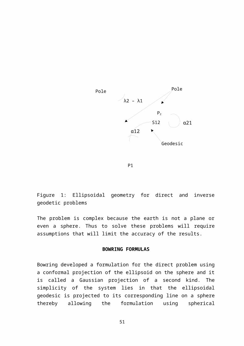
Figure 1: Ellipsoidal geometry for direct and inverse geodetic problems

The problem is complex because the earth is not a plane or even a sphere. Thus to solve these problems will require assumptions that will limit the accuracy of the results.

BOWRING FORMULAS

Bowring developed a formulation for the direct problem using a conformal projection of the ellipsoid on the sphere and it is called a Gaussian projection of a second kind. The simplicity of the system lies in that the ellipsoidal geodesic is projected to its corresponding line on a sphere thereby allowing the formulation using spherical trigonometry. Both the direct and inverse solutions are non-iterative. These formulas are valid for lines up to 150km.

Without derivation, the common equations used by Bowring are:

A = √¿¿)

B = √(1+e '2 cos2 φ1¿)¿

C = √(1+e '2¿)¿

w = A (λ2−λ1)

2

Direct ProblemThen the formulas for the direct problem are presented as follows:

37

P2

σ = s B2

aC

λ2 = λ1 + 1A

tan−1( A tanσ sin α 12

Bcos φ1−tanσ sin φ1cos α12)

D = 12

sin−1[ sinσ (cosα 12−1A

sin φ1 sin α12 tanw)]φ2 = φ1 + 2D[B−3

2e ' 2 Dsin (2 φ1+

43

BD )]α12 = tan−1[ −Bsin α12

cosσ (tanσ tan φ1−Bcos α12 ) ]Inverse ProblemThe inverse problem begins by computing a series of constant values:

D = ∆ φ2 B [1+3 e '2

4 B2 ∆ φsin(2 φ1+23

∆ φ)]E = sinD cosw

F = 1A

sinw¿)

tanG = FA

sin( σ2 ) = (E2 + F2)1/2

tanH = 1A (sin φ1+Bcos φ1tanD )tanw

Then, the inverse geodetic values, azimuth and distance, are found using the following relationships:

α12 = G – H

α21 = G + H ± 180

38

s = aCσB2

GAUSS MID-LATITUDE FORMULA

This approach was first published in English in 1861. This method is based on spherical approximations of the earth. This method is based on using spherical approximations of the earth. Thus, azimuths is not true. Thus, this method is best used for distances less than 40km at latitudes less than 800.

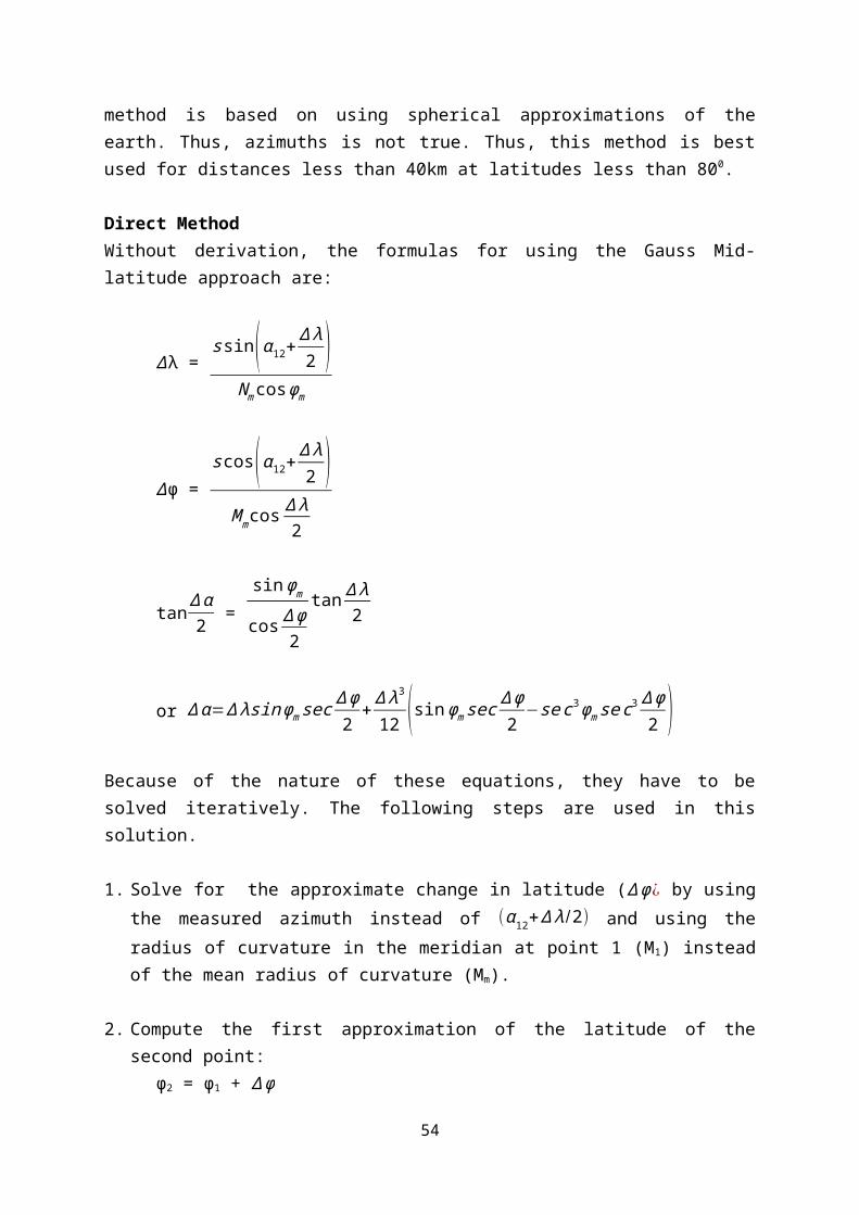
Direct MethodWithout derivation, the formulas for using the Gauss Mid-latitude approach are:

∆λ = ssin (α 12+

∆ λ2 )

N mcos φm

∆φ = s cos(α12+

∆ λ2 )

M m cos ∆ λ2

tan∆ α2 =

sin φm

cos ∆ φ2

tan ∆ λ2

or ∆ α=∆ λsin φm sec ∆ φ2

+ ∆ λ3

12 (sin φm sec ∆ φ2

−se c3φm se c3 ∆ φ2 )

Because of the nature of these equations, they have to be solved iteratively. The following steps are used in this solution.

1. Solve for the approximate change in latitude (∆ φ¿ by using the measured azimuth instead of (α 12+∆ λ/2) and using the radius of curvature in the meridian at point 1 (M1) instead of the mean radius of curvature (Mm).

2. Compute the first approximation of the latitude of the second point:φ2 = φ1 + ∆ φ

3. Determine the first approximation of the change in longitude and the longitude of the second point.

39

λ2 = λ1 + ∆λ

4. Find the first approximation of the change in azimuth.

5. Using these steps approximations, update the values M, N, φm and other values listed in the first four steps.

Inverse ProblemThe Gauss Mid-Latitude formulae for the inverse problem can be developed into direct computation requiring no iteration. It can be presented as follows (without derivation):

s = s1 [ s1

2 N m

sin ( s1

2 Nm ) ]α12 = tan−1( X1

X2)−∆ α

2

α21 = α12 + ∆α ± 1800

where, s1 = ( X12+ X2

2 )1/2,

Then,

X1 = s1sin(α12+∆ α2 ) = Nm ∆λ’cosφm

X2 = s1cos(α12+∆ α2 ) = Mm ∆φ’cos( ∆ λ

2 )

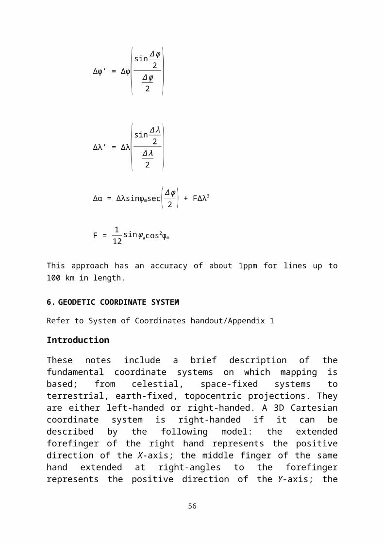
∆φ’ = ∆φ( sin ∆ φ2

∆ φ2

)∆λ’ = ∆λ( sin ∆ λ

2∆ λ2

)40

∆α = ∆λsinφmsec( ∆ φ2 ) + F∆λ3

F = 112

sin φmcos2φm

This approach has an accuracy of about 1ppm for lines up to 100 km in length.

6. GEODETIC COORDINATE SYSTEM

Refer to System of Coordinates handout/Appendix 1

Introduction

These notes include a brief description of the fundamental coordinate systems on which mapping is based; from celestial, space-fixed systems to terrestrial, earth-fixed, topocentric projections. They are either left-handed or right-handed. A 3D Cartesian coordinate system is right-handed if it can be described by the following model: the extended forefinger of the right hand represents the positive direction of the X-axis; the middle finger of the same hand extended at right-angles to the forefinger represents the positive direction of the Y-axis; the extended thumb of the right hand, perpendicular to them both, represents the positive direction of the Z-axis.

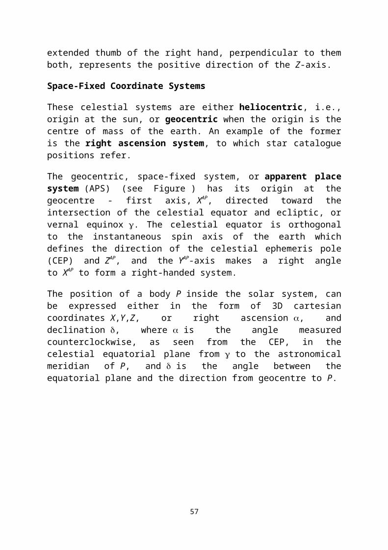
Space-Fixed Coordinate Systems

These celestial systems are either heliocentric, i.e., origin at the sun, or geocentric when the origin is the centre of mass of the earth. An example of the former is the right ascension system, to which star catalogue positions refer.

The geocentric, space-fixed system, or apparent place system (APS) (see Figure ) has its origin at the geocentre - first axis, XAP, directed toward the intersection of the celestial equator and ecliptic, or vernal equinox . The celestial equator is orthogonal to the instantaneous spin axis of the earth which defines the direction of the celestial ephemeris pole (CEP) and ZAP, and the YAP-axis makes a right angle to XAP to form a right-handed system.

The position of a body P inside the solar system, can be expressed either in the form of 3D cartesian coordinates X,Y,Z, or right ascension , and declination , where  is the angle measured counterclockwise, as seen from the CEP, in the celestial equatorial plane from  to the astronomical meridian of P, and  is the angle between the equatorial plane and the direction from geocentre to P.

41

Figure 1: Space-Fixed Coordinate System

Earth-Fixed Coordinate Systems

The usual and most important example of these is the conventional terrestrial system (CTS) (Figure ), which is also right-handed with the origin at the geocentre and the ZCT-axis directed towards the conventional terrestrial pole (CTP), formerly CIO, which is referenced by means of the polar motion coordinates xp, yp (see section ). The conventional terrestrial equator is orthogonal to the direction of the CTP, and contains the XCT-axis defined by the intersection of the equator with the Greenwich Meridian, and the YCT-axis, completing the system. The position of a point P on the terrain surface can be represented very simply by 3D cartesion coordinates XP,YP,ZP.

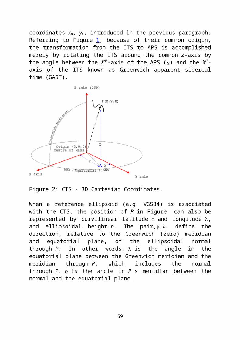
Another important system, for computational purposes, is the instantaneous terrestrial system (ITS), which differs from the CTS only in so far as its ZIT-axis is parallel to the instantaneous rather than conventional spin axis. The ZIT-axis of the ITS wobbles around the CTP, and this movement is described by the polar motion coordinates xp, yp, introduced in the previous paragraph. Referring to Figure 1, because of their common origin, the transformation from the ITS to APS is accomplished merely by rotating the ITS around the common Z-axis by the angle between the XAP-axis of the APS () and the XIT-axis of the ITS known as Greenwich apparent sidereal time (GAST).

42

Figure 2: CTS - 3D Cartesian Coordinates.

When a reference ellipsoid (e.g. WGS84) is associated with the CTS, the position of P in Figure  can also be represented by curvilinear latitude  and longitude , and ellipsoidal height h. The pair,,, define the direction, relative to the Greenwich (zero) meridian and equatorial plane, of the ellipsoidal normal through P. In other words,  is the angle in the equatorial plane between the Greenwich meridian and the meridian through P, which includes the normal through P.  is the angle in P's meridian between the normal and the equatorial plane.

Figure 3: CTS - Geodetic , Coordinates.

Non-Geocentric Coordinate System

43

The Figure 4 illustrates the relationship (exaggerated !) between the CTS and its associated ellipsoid, and a typical geodetic system which is not geocentric but is chosen to fit the geoid optimally in a particular region of the globe. The ZG-axis of the geodetic system which coincides with the minor axis of the geodetic ellipsoid, is generally oriented to be parallel with the ZCT-axis of the CTS system.

Figure 4: CTS and Geodetic (non-geocentric) System

Polar Motion

Polar motion refers to the motion of the spin axis of the earth with respect to the crust (Figure ). The path of the spin-axis between the years 1984-1987 is shown in the diagram above, and can be seen to be periodic to an extent, with a period of about 434 days and an amplitude of less than 10m. The mean position of the spin-axis for the years 1900-1905 is taken to be the CTP and there appears to be a gradual wandering of the centre of the figure away from the CTP.

44

Figure 5: Polar Motion

Topocentric Coordinate Systems

The local systems are topocentric. The local geodetic system (LGS) has its zLG-axis coinciding with the ellipsoidal normal. The xLG-axis points towards the geodetic north pole and the yLG-axis points east to complete a left-handed system (Figure ).

Figure 6: Local Topocentric (Geodetic) System

The zLA-axis of the local astronomic system (LAS) coincides with the plumbline through P and is therefore normal to the geoidal surface. The xLA-axis is directed

45

towards the CTP and the y-axis again completes a left-handed system. The CTS and LAS constitute a natural pair, while the local astronomic and local geodetic systems are related through deflections of the vertical (z-axis) and Laplace equation (x-axis). The LAS is the system in which astronomical observations are made.

(Deflection of the vertical is the spatial angle between the direction of the plumbline( or earth's gravity vector) on the geoid and the direction of the ellipsoidal normal. It is convenient to decompose the angle into two orthogonal components , , called the deflection components, where  is in the meridian plane and  is in the prime vertical. The sign of the components is taken to be positive if the gravity vector is north and east of the geodetic vertical.)

Projections

Only two projections are used in Zimbabwe: Universal Transverse Mercator (UTM) and Gauss. The Following notes compare the two (Figure ).

Figure 7: UTM/Gauss Projection

1. The UTM and Gauss projections are both transverse Mercator projections which have the property of conformality or isomorphism, and so the equations transforming points from the ellipsoidal surface to the plane and back are essentially the same. The transverse Mercator projection uses a projection cylinder whose axis is imagined to be parallel to the earth's equatorial plane and perpendicular to its spin axis. In the case of Gauss, it touches the ellipsoid along a central meridian, but in the case of UTM it intersects the ellipsoid along lines parallel to the central meridian. After the cylinder is developed (i.e. opened), all the projected meridians and parallels become curved lines.

46

2. Conformality or orthomorphism is the property whereby the scale at any point on the projected surface is the same in all directions. For this reason directions at a point on the earth's surface to nearby surrounding points, are for all practical purposes left undistorted by projection.

3. The UTM belt is 6 degrees wide, 3 degrees either side of the central meridian which in the case of Zimbabwe coincides with 27 and 33 degrees east. The Gauss belt is 2 degrees wide, 1 degree either of the central meridian which is chosen to be any one of the odd-numbered lines of longitude - 25, 27, 29, 31, 33 (Figure ).

4. The scale factor for Gauss is unity on the central meridian and 0.9996 for UTM

5. The origin for the Gauss coordinate system is the intersection of the central meridian with the equator; i.e. x = 0 on the equator increasing south and y = 0 on the central meridian increasing towards the west. UTM has a false northing of 10 000000m at the equator increasing northwards and a false easting of 500 000m on the central meridian increasing eastwards.

6. In Zimbabwe the UTM projection is used for mapping whilst the Gauss projection is used mainly for cadastral beacon coordinates because of the relatively small scale factor at the edges of a 2 degree belt.

Figure 8: Gauss 2-Degree and UTM 6-Degree panels

Variations in Coordinate Systems

Factors affecting the coordinate systems:

Proper motion

47

The small motion of stars relative to each other and to inertial space.Proper motion is divided into two components:Radial - along the heliocentric vectorTangential - along the tangential vector, affects coordinate systems the most

Precession

The Earth's rotation axis is not fixed in space. Like a rotating toy top, the direction of the rotation axis executes a slow precession with a period of 26,000 years (see following figure).

Pole Stars are TransientThus, Polaris will not always be the Pole Star or North Star. The Earth's rotation axis happens to be pointing almost exactly at Polaris now, but in 13,000 years the precession of the rotation axis will mean that the bright star Vega in the constellation Lyra will be approximately at the North Celestial Pole, while in 26,000 more years Polaris will once again be the Pole Star.

Precession of the EquinoxesSince the rotation axis is precessing in space, the orientation of the Celestial Equator also precesses with the same period. This means that the position of the equinoxes is changing slowly with respect to the background stars. This precession of the equinoxes means that the

48

right ascension and declination of objects changes very slowly over a 26,000 year period. This effect is negligibly small for casual observing, but is an important correction for precise observations.

The Dawning of the Age of Aquarius (Almost)Because of the precession of the equinoxes, the vernal equinox moves through all the constellations of the Zodiac over the 26,000 year precession period. Presently the vernal equinox is in the constellation Pisces and is slowly approaching Aquarius.

The Vernal Equinox

Annual Parallax

Parallax is a displacement or difference in the apparent position of an object viewed along two different lines of sight, and is measured by the angle or semi-angle of inclination between those two lines. The term is derived from the Greek παράλλαξις (parallaxis), meaning "alteration". Nearby objects have a larger parallax than more distant objects when observed from different positions, so parallax can be used to determine distances.

The apparent displacement of an observed object due to a change in the position of the observer. Astronomy - the apparent angular displacement of a celestial body due to its being observed from the surface instead of from the center of the earth (diurnal parallax or  geocentric parallax) or due to its being observed from the earth instead of from the sun (annual parallax or  heliocentric parallax)

Annual Aberration

49

The small displacement in position of a star's image during the year due to the motion of the Earth around the Sun. Annual aberration was discovered by J. Bradley in 1728 from observations of the changes in distance from the zenith of the star Gamma Draconis. The ratio of the Earth's mean velocity to the speed of light gives the constant of aberration, 20″.5. This is the maximum amount by which a star can appear to be displaced from its mean position. During the course of a year, the star appears to move around its mean position in a shape that ranges from a circle for a star at the ecliptic pole, via a progressively flattened ellipse, to a straight line for a star on the ecliptic.

The aberration of light (also referred to as astronomical aberration or stellar aberration) is an astronomical phenomenon which produces an apparent motion of celestial objects.

The aberration of light (also referred to as astronomical aberration or stellar aberration) is an astronomical phenomenon which produces an apparent motion of celestial objects. It was discovered and later explained by the third Astronomer Royal, James Bradley, in 1725, who attributed it to the finite speed of light and the motion of Earth in its orbit around the Sun.

At the instant of any observation of an object, the apparent position of the object is displaced from its true position by an amount which depends upon the transverse component of the velocity of the observer, with respect to the vector of the incoming beam of light (i.e., the line actually taken by the light on its path to the observer). In the case of an observer on Earth, the direction of its velocity varies during the year as Earth revolves around the Sun (or strictly speaking, the barycenter of the solar system), and this in turn causes the apparent position of the object to vary. This particular effect is known as annual aberration or stellar aberration, because it causes the apparent position of a star to vary periodically over the course of a year. The maximum amount of the aberrational displacement of a star is approximately 20 arcseconds in right ascension or declination. Although this is a relatively small value, it was well within the observational capability of the instruments available in the early eighteenth century.

Aberration should not be confused with stellar parallax, although it was an initially fruitless search for parallax that first led to its discovery. Parallax is caused by a change in the position of the observer looking at a relatively nearby object, as measured against more distant objects, and is therefore dependent upon the distance between the observer and the object.

50

In contrast, stellar aberration is independent of the distance of a celestial object from the observer, and depends only on the observer's instantaneous transverse velocity with respect to the incoming light beam, at the moment of observation. The light beam from a distant object cannot itself have any transverse velocity component, or it could not (by definition) be seen by the observer, since it would miss the observer. Thus, any transverse velocity of the emitting source plays no part in aberration. Another way to state this is that the emitting object may have a transverse velocity with respect to the observer, but any light beam emitted from it which reaches the observer, cannot, for it must have been previously emitted in such a direction that its transverse component has been "corrected" for. Such a beam must come "straight" to the observer along a line which connects the observer with the position of the object when it emitted the light.

Aberration should also be distinguished from light-time correction, which is due to the motion of the observed object, like a planet, through space during the time taken by its light to reach an observer on Earth. Light-time correction depends upon the velocity and distance of the emitting object during the time it takes for its light to travel to Earth. Light-time correction does not depend on the motion of the Earth—it only depends on Earth's position at the instant when the light is observed. Aberration is usually larger than a planet's light-time correction except when the planet is near quadrature (90° from the Sun), where aberration drops to zero because then the Earth is directly approaching or receding from the planet. At opposition to or conjunction with the Sun, aberration is 20.5" while light-time correction varies from 4" for Mercury to 0.37" for Neptune (the Sun's light-time correction is less than 0.03").

It has been stated above that aberration causes a displacement of the apparent position of an object from its true position. However, it is important to understand the precise technical definition of these terms.

The apparent position of a star or other very distant object is the direction in which it is seen by an observer on the moving Earth. The true position (or geometric position) is the direction of the straight line between the observer and star at the instant of observation. The difference between these two positions is caused mostly by aberration.

Aberration occurs when the observer's velocity has a component that is perpendicular to the line traveled by light between the star and observer. In Figure 1 to the right, S represents the spot where the star light enters the telescope, and E the position of the eye piece. If the telescope does not move, the true direction of the star relative to the observer can be found by following the line ES. However, if Earth, and therefore the eye piece of the telescope, moves from E to E’ during the time it takes light to travel from S to E, the star will no longer appear in the center of the eye piece. The telescope must therefore be adjusted so that the star light enters the telescope at spot S’. Now the star light will travel along the line S’E’ and reach E’ exactly when the moving eye piece also reaches E’. Since the telescope has been adjusted by the angle SES’, the star's apparent position is hence displaced by the same angle.

Many find aberration to be counter-intuitive, and a simple thought experiment based on everyday experience can help in its understanding. Imagine you are standing in the rain. There is no wind, so the rain is falling vertically. To protect yourself from the rain you hold an umbrella directly above you.

51

Now imagine that you start to walk. Although the rain is still falling vertically (relative to a stationary observer), you find that you have to hold the umbrella slightly in front of you to keep off the rain. Because of your forward motion relative to the falling rain, the rain now appears to be falling not from directly above you, but from a point in the sky somewhat in front of you.

The deflection of the falling rain is greatly increased at higher speeds. When you drive a car at night through falling rain, the rain drops illuminated by your car's headlights appear to (and actually do) fall from a position in the sky well in front of your car.

According to the special theory of relativity, the aberration only depends on the relative velocity v between the observer and the star. Thus, the aberration of light does not imply an absolute frame of reference, as when one moves in the rain. The speed of the rain perceived in a running car is increased as it hits the windscreen more heavily. Instead, according to the special theory of relativity, the speed of light is constant and only its direction changes. The above formula accounts for that while the simpler tan(?-?’)=v/c does not.

In most cases the transverse velocity of the star is unknown. However, for some binary systems where a high rotating speed can be inferred, it doesn't cause an aberration as apparently implied by the relativity principle. As discussed above, the reason why the observer motion results in the aberration inherent in crossing parallel beams of light coming from the star. Instead, the star moves with the divergent beams of light that itself originates in all directions, and its motion just selects which one is destined to hit the observer. Indeed, dependency on the source is paradoxical: Consider a second source of light that on a given instant coincides with the star, but is not at rest with it. Suppose that two rays of light reach the observer, one emitted by the star and the other by the second source in the instant when they coincide. If rays are straight, since they share two points (the coinciding sources and the observer) then they must coincide. However, since the velocities of the sources differ, the observer would see those rays coming from different directions, if aberration depended on the source's motion.

There are a number of types of aberration, caused by the differing components of the Earth's motion:

Annual aberration is due to the revolution of the Earth around the Sun.

Planetary aberration is the combination of aberration and light-time correction.

Diurnal aberration is due to the rotation of the Earth about its own axis.

Secular aberration is due to the motion of the Sun and solar system relative to other stars in the galaxy.

52

7. COORDINATE TRANSFORMATIONS

Coordinate transformations are used in surveying and mapping to transform coordinates in one system to coordinate in another system, and take many forms. For example:

map projections are transformations of geographical coordinates, latitude ɸ and longitude λ on a sphere or ellipsoid, to rectangular (or Cartesian) coordinates on a plane.

Polar-Rectangular conversions where coordinates of points in polar coordinates, say bearings and distances, are converted to rectangular coordinates

2D transformations where the coordinates of points in one rectangular system (x, y) are transformed into coordinates in another rectangular system (X, Y).

3D transformation where coordinates of points in one right-handed rectangular system (x, y, z) are transformed into another rectangular system (X, Y, Z).

The effect of a transformation on a group of points defining a 2D polygon or 3D object varies from simple changes of location and orientation (without any change in shape or size to uniform scale change (no change in shape) and finally to changes in shape and size of different degrees of non-linearity (Mikhail 1976).

3D transformations3D transformations also include transformations from geographical coordinates (ɸ, λ, h) on a reference surface (sphere or ellipsoid), to rectangular coordinates (X, Y, Z) whose origin is at the centre of the reference surface, or to a local rectangular system (E, N, U) whose origin is a point on the reference surface.Similar to the 2D case, affine transformation in 3D can be factored out in several elementary transformations:

translation uniform scale non-uniform scale reflections

However, we limit consideration to the seven-parameter transformation used extensively in Geodesy. This is composed of:

translation uniform scale three rotations

Rotations of 3D coordinate system

There are 3 elementary rotations, one about each of the three axes, They are frequently performed in sequence one after the other. The rotations are as follows:

i. ε about the x-axis, that is changing the Y-Z plane

53

ψ ωε

Z

Y

X

Z'

Y'

P

ycosε

ysinε zsinε

zcosε

y

z

ε

ε

ii. ψ about the y-axis, that is changing the X-Z planeiii. ω about the z-axis, that is changing the X-Y plane

(xa, ya, za) (x', y', z') (x'', y'', z'') (x, y, z)

Rotation about x axis through angle ε

x' = xy' = ycosε + zsinεz' = -ysinε + zcosε

in matrix form the above equations can be written as:

x 'y 'z '

= 1 0 00 cosε sinε0 −sinε cosε

xyz

Rx (ε) = 1 0 00 cosε sinε0 −sinε cosε

54

Rotation about y axis through angle ψ

x' = xcosψ - zsin ψy' = yz' = zcos ψ + xsin ψ

Ry(ψ) = cosψ 0 −sinψ

0 1 0sin ψ 0 cosψ

Rotation about z axis through angle ω

55

Rz(ω) = cosω sinω 0

−sinω cosω 00 0 1

The product of the three consecutive orthogonal rotations is:

R = cosψ cosω cosε sinω+sinε sinψ cosω sinε sinω−cosε sinψ cosω

−cosψ sinω cosε cosω−sinε sinψ sinω sinε cosω+cosε sinψ sinωsinψ −sinε cosψ cosε cosψ

Seven-parameter transformationThis transformation contains seven parameters: a uniform scale change (Δ), three rotations (ε, ψ, ω) and three translations (Δx, Δy, Δz). The general form of the equation becomes:

y = (Δ) (R) (x) + t

Because the rotation angles will generally be small R(above) can be simplified to:

56

R = I + Q

= 1 0 00 1 00 0 1

+0 ω −ψ

−ω 0 εψ −ε 0

By neglecting the 2nd order terms in Δ and in ε, ψ, ω the linearised version of the vector transformation equation can be written as:

T + u +Δu + Qu - X = 0Each station yields one such vector equation, f = V - Ax + f = 0, where:

V = vector of residuals in u, v, and w

A = design matrix of coefficients ∂ y∂ x

x = unknown transformation parametres (initially set to 0)

and f = xyz

- uvw

Thus we get;

v1v2v3

=

57

h

H

ɸ

ɸ

Transformations from Geodetic (φ, λ, h) to Geocentric (X, Y, Z)

X = (N + h) cosφ cosλY = (N + h) cosφ sinλZ = [N(1 - e2) + h] sinφ

Transformations from Geocentric (X, Y, Z) to Geodetic (φ, λ, h)This transformation is not straight forward, it is iterative.

Longitudeλ = tan-1(Y/Z)

LatitudeInitial approximation for N and φ

tan(φ) = ( N+h ) sinφ

√ x2+ y2 .........................................1

(N + h) sinφ = z + e2N sinφ .........................2

tan(φ) = z+e2Nsinφ

√x2+ y2 ...........................................3

φ0 = tan-1(z

(1−e 2)√ x2+ y) ...................................4

using this value for the latitude, an initial approximation for the value of N can be found as:

58

N0 = a

√1−e2 sin 2φ .............................................5

Now substitute the values obtained in equations 4 and 5, back into equation 3 and iterate until sufficient convergence is obtained for the station's latitude.

Ellipsoidal heightFrom equation 1 we have

cosφ = √x2+ y2

N+h

h = √x2+ y2

cosφ + N

59