aster users handbook - unlp · 2004-07-16 · aster users handbook photo-diode monitors the...
TRANSCRIPT


ASTER Users Handbook
ASTER User Handbook
Version 1
Michael Abrams Simon Hook
Jet Propulsion Laboratory 4800 Oak Grove Dr. Pasadena, CA 91109
2

ASTER Users Handbook
Acknowledgments
This document was prepared at the Jet Propulsion Laboratory/California Institute of Technology. Work was performed under contract to the National Aeronautics and Space Administration.
3

ASTER Users Handbook
Table of Contents
1. ASTER........................................................................................................................................ 6 2. The ASTER Instrument .............................................................................................................. 6
2.1 The VNIR Instrument ........................................................................................................... 9 2.2 The SWIR Instrument ......................................................................................................... 10 2.3 The TIR Instrument............................................................................................................. 10
3. Level 1 Data Products............................................................................................................... 12 3.1 Level 1A Data Product........................................................................................................ 12 3.2 Level 1B Data Product........................................................................................................ 15
4. ASTER Higher-Level Products ................................................................................................ 18 5. Radiometric Parameters ............................................................................................................ 19 6. Data Acquisition ....................................................................................................................... 21
6.1 Data Acquisition Strategy ........................................................................................... 21 6.2 Search and Order Data Products ......................................................................................... 22 6.3. Ordering Level 2 Products ................................................................................................. 30 6.4 Data Acquisition Requests.................................................................................................. 30
7. Application Examples............................................................................................................... 30 7.1 Cuprite, Nevada............................................................................................................. 30 7.2 Lake Tahoe.......................................................................................................................... 34
8. Frequently asked questions ....................................................................................................... 43 9. Software Availability ................................................................................................................ 47 Appendix I. Dump of HDF metadata in L1B file ......................................................................... 48 Appendix II. Higher Level Data Products. ................................................................................... 56 Appendix III: Metadata Cross Reference Table ........................................................................... 73 Appendix IV. Data sets available through EDC ........................................................................... 92
4

ASTER Users Handbook
List of Figures
Figure 1 The ASTER instrument before launch ............................................................................. 7 Figure 2 Diagrams of the 3 optical assemblies for the VNIR, SWIR and TIR instruments........... 8 Figure 3. Comparison of spectral bands for ASTER and Landsat Thematic Mapper. %Ref is
reflectance percent. ................................................................................................................. 9 Figure 4. Flow of ASTER data between US and Japan................................................................ 12 Figure 5. Five levels of HDF information in the ASTER Level 1A data product. ....................... 14 Figure 6. Five levels of HDF information in the ASTER Level 1B data product. ....................... 16 Figure 7. Cuprite Mining District, Nevada displayed using ASTER SWIR bands 4-6-8 as a RGB
composite. Area covered is 15 x 20 km................................................................................ 31 Figure 8. Spectral Angle Mapper classification of Cuprite SWIR data. blue=kaolinite;
red=alunite; light green=calcite; dark green=alunite+kaolinite; cyan=montmorillonite; purple=unaltered; yellow=silica or dickite. .......................................................................... 32
Figure 9. ASTER image spectra (left) and library spectra(right) for minerals mapped at Cuprite................................................................................................................................................ 33
Figure 10. Outline map of Lake Taoe CA/NV ............................................................................. 34 Figure 11. Raft measurementss..................................................................................................... 35 Figure 12. Field measurements at the USCG................................................................................ 37 Figure 13. Color Infrared Composite of ASTER bands 3,2,1 as R,G,B respectively. Red areas
indicate vegetation, white areas are snow............................................................................. 38 Figure 14. ASTER band 1 (0.52-0.60um) color coded to show variations in the intensity of the
near-shore bottom reflectance............................................................................................... 39 Figure 15. Bathymetric map of Lake Tahoe CA/NV.................................................................... 40 Figure 16. Near-shore clarity map derived from ASTER data and a bathymetric map................ 40 Figure 17. ASTER band 13 brightness temperature image of Lake Tahoe acquired June 3, 2001.
............................................................................................................................................... 42
List of Tables
Table 1. ASTER subsystem characteristics. ................................................................................... 8 Table 2. Resampling methods and projections available for producing Level 1B products. ....... 17 Table 3. ASTER higher level standard data products................................................................... 18 Table 4. Maximum radiance values for all ASTER bands and all gains. ..................................... 19 Table 5 Calculated Unit Conversion Coefficients ........................................................................ 20
5

ASTER Users Handbook
1. ASTER
The Advanced Spaceborne Thermal Emission and Relfection Radiometer (ASTER) is an advanced multispectral imager that was launched on board NASA’s Terra spacecraft in December, 1999. ASTER covers a wide spectral region with 14 bands from the visible to the thermal infrared with high spatial, spectral and radiometric resolution. An additional backward-looking near infrared band provides stereo coverage. The spatial resolution varies with wavelength: 15 m in the visible and infrared (VNIR), 30 m in the short wave infrared (SWIR), and 90 m in the thermal infrared (TIR). Each ASTER scene covers an area of 60 x 60 km.
Terra is the first of a series of multi-instrument spacecraft forming NASA’s Earth Observing System (EOS). EOS consists of a science component and a data system supporting a coordinated series of polar-orbiting and low inclination satellites for long-term global observations of the land surface, biosphere, solid Earth, atmosphere, and oceans. By enabling improved understanding of the Earth as an integrated system, the EOS program has benefits for us all. In addition to ASTER, the other instruments on Terra are the Moderate-Resolution Imaging Spectroradiometer (MODIS), Multi-angle Imaging Spectro-Radiometer (MISR), Clouds and the Earth’s Radiant Energy System (CERES), and Measurements of Pollution in the Troposphere (MOPITT). As the only high spatial resolution instrument on Terra, ASTER is the “zoom lens” for the other instruments. Terra is in a sun-synchronous orbit, 30 minutes behind Landsat ETM+; it views the surface at about 10:30am local solar time.
ASTER can acquire data over the entire globe with an average duty cycle of 8% per orbit. This translates to acquisition of about 650 scenes per day, that are processed to Level 1A; of these, about 150 are processed to Level 1B. All 1A and 1B scenes are transferred to the EOSDIS archive at the Eros Data Center Distributed Active Archive Center (EDCDAAC), for storage, distribution, and processing to higher level data products. All ASTER data products are stored in Hierarchical Data Format (HDF).
2. The ASTER Instrument
ASTER is a cooperative effort between NASA and Japan's Ministry of Economy Trade and
Industry (METI) formerly known as Ministry of International Trade and Industry (MITI), with the collaboration of scientific and industry organizations in both countries. The ASTER instrument consists of three separate instrument subsystems (Figure 1).
6

ASTER Users Handbook
Figure 1 The ASTER instrument before launch Each subsystem operates in a different spectral region, has its own telescope(s), and is built
by a different Japanese company. ASTER consists of three different subsystems (Figure 2): the Visible and Near Infrared (VNIR) has three bands with a spatial resolution of 15 m, and an additional backward telescope for stereo; the Shortwave Infrared (SWIR) has 6 bands with a spatial resolution of 30 m; and the Thermal Infrared (TIR) has 5 bands with a spatial resolution of 90 m. The spectral bandpasses are shown in Table 1, and a comparison of bandpasses with Landsat Thematic Mapper is shown in Figure 3. In addition, one more telescope is used to see backward in the near infrared spectral band (band 3B) for stereoscopic capability.
7

ASTER Users Handbook
Figure 2 Diagrams of the 3 optical assemblies for the VNIR, SWIR and TIR instruments. Table 1. ASTER subsystem characteristics.
Subsystem Band
No. Spectral Range (um) Spatial
Resolution, m Quantization Levels
1 0.52-0.60 2 0.63-0.69 3N 0.78-0.86
VNIR
3B 0.78-0.86
15
8 bits
4 1.60-1.70 5 2.145-2.185 6 2.185-2.225 7 2.235-2.285 8 2.295-2.365
SWIR
9 2.360-2.430
30
8 bits
10 8.125-8.475 11 8.475-8.825 12 8.925-9.275 13 10.25-10.95
TIR
14 10.95-11.65
90
12 bits
8

ASTER Users Handbook
Figure 3. Comparison of spectral bands for ASTER and Landsat Thematic Mapper. %Ref is reflectance
percent. The Terra spacecraft is flying in a circular, near-polar orbit at an altitude of 705 km. The
orbit is sun-synchronous with equatorial crossing at local time of 10:30 a.m., returning to the same orbit every 16 days. The orbit parameters are the same as Landsat 7, except for the local time.
2.1 The VNIR Instrument
The VNIR subsystem consists of two independent telescope assemblies to minimize image
distortion in the backward and nadir looking telescopes (Figure 2). The detectors for each of the bands consist of 5000 element silicon charge coupled detectors (CCD's). Only 4000 of these detectors are used at any one time. A time lag occurs between the acquisition of the backward image and the nadir image. During this time earth rotation displaces the image center. The VNIR subsystem automatically extracts the correct 4000 pixels based on orbit position information supplied by the EOS platform.
The VNIR optical system is a reflecting-refracting improved Schmidt design. The backward looking telescope focal plane contains only a single detector array and uses an interference filter for wavelength discrimination. The focal plane of the nadir telescope contains 3 line arrays and uses a dichroic prism and interference filters for spectral separation allowing all three bands to view the same area simultaneously. The telescope and detectors are maintained at 296 ± 3K using thermal control and cooling from a platform provided cold plate. On-board calibration of the two VNIR telescopes is accomplished with either of two independent calibration devices for each telescope. The radiation source is a halogen lamp. A diverging beam from the lamp filament is input to the first optical element (Schmidt corrector) of the telescope subsystem filling part of the aperture. The detector elements are uniformly irradiated by this beam. In each calibration device, two silicon photo-diodes are used to monitor the radiance of the lamp. One
9

ASTER Users Handbook
photo-diode monitors the filament directly and the second monitors the calibration beam just in front of the first optical element of the telescope. The temperature of the lamp base and the photo-diodes is also monitored. Provision for electrical calibration of the electronic components is also provided.
The system signal-to-noise is controlled by specifying the NE delta rho to be < 0.5% referenced to a diffuse target with a 70% albedo at the equator during equinox. The absolute radiometric accuracy is to be ± 4% or better.
The VNIR subsystem produces by far the highest data rate of the three ASTER imaging subsystems. With all four bands operating (3 nadir and 1 backward) the data rate including image data, supplemental information and subsystem engineering data is 62 Mbps.
2.2 The SWIR Instrument
The SWIR subsystem uses a single aspheric refracting telescope (Figure 2). The detector in
each of the six bands is a Platinum Silicide-Silicon (PtSi-Si) Schottky barrier linear array cooled to 80K. Cooling is provided by a split Stirling cycle cryocooler with opposed compressors and an active balancer to compensate for the expander displacer. The on-orbit design life of this cooler is to be 50,000 hours. Although ASTER operates with a low duty cycle (8% average data collection time) the cryocooler operates continuously because the cool-down and stabilization time is long. No cyrocooler has yet demonstrated this length of performance, and the development of this long-life cooler was one of several major technical challenges faced by the ASTER team.
The cryocooler is a major source of heat. Because the cooler is attached to the SWIR telescope, which must be free to move to provide cross-track pointing, this heat cannot be removed using a platform provided cold plate. This heat is transferred to a local radiator attached to the cooler compressor and radiated to space.
Six optical bandpass filters are used to provide spectral separation. No prisms or dichroic elements are used for this purpose. A calibration device similar to that used for the VNIR subsystem is used for inflight calibration. The exception is that the SWIR subsystem has only one such device.
The NE delta rho will vary from 0.5 to 1.3% across the bands from short to long wavelength. The absolute radiometric accuracy is to be +4% or better. The combined data rate for all six SWIR bands, including supplementary telemetry and engineering telemetry, is 23 Mbps.
2.3 The TIR Instrument
The TIR subsystem uses a Newtonian catadioptric system with an aspheric primary mirror
and lenses for aberration correction (Figure 2). Unlike the VNIR and SWIR telescopes, the telescope of the TIR subsystem is fixed with pointing and scanning done by a mirror. Each band uses 10 Mercury-Cadmium-Telluride (HgCdTe) detectors in a staggered array with optical band-pass filters over each detector element. Each detector has its own pre-and post-amplifier for a total of 50.
As with the SWIR subsystem, the TIR subsystem uses a mechanical split Stirling cycle cooler for maintaining the detectors at 80K. In this case, since the cooler is fixed, the waste heat it generates is removed using a platform supplied cold plate.
10
ASTER Users Handbook
The scanning mirror functions both for scanning and pointing. In the scanning mode the mirror oscillates at about 7 Hz. For calibration, the scanning mirror rotates 180 degrees from the nadir position to view an internal black body which can be heated or cooled. The scanning/pointing mirror design precludes a view of cold space, so at any one time only a one point temperature calibration can be effected. The system does contain a temperature controlled and monitored chopper to remove low frequency drift. In flight, a single point calibration can be done frequently (e.g., every observation) if necessary. On a less frequent interval, the black body may be cooled or heated (to a maximum temperature of 340K) to provide a multipoint thermal calibration. Facility for electrical calibration of the post-amplifiers is also provided.
For the TIR subsystem, the signal-to-noise can be expressed in terms of an NE delta T. The requirement is that the NE delta T be less than 0.3K for all bands with a design goal of less than 0.2K. The signal reference for NE delta T is a blackbody emitter at 300K. The accuracy requirements on the TIR subsystem are given for each of several brightness temperature ranges as follows: 200 - 240K, 3K; 240 - 270K, 2K; 270 - 340K, 1K; and 340 - 370K, 2K.
The total data rate for the TIR subsystem, including supplementary telemetry and engineering telemetry, is 4.2 Mbps. Because the TIR subsystem can return useful data both day and night, the duty cycle for this subsystem has been set at 16%. The cryocooler, like that of the SWIR subsystem, operates with a 100% duty cycle.
11

ASTER Users Handbook
3. Level 1 Data Products
The ASTER instrument has two types of Level 1 data: Level 1A (L1A) and Level 1B (L1B). L1A data are formally defined as reconstructed, unprocessed instrument data at full resolution. The ASTER L1A data consist of the image data, the radiometric coefficients, the geometric coefficients and other auxiliary data without applying the coefficients to the image data, thus maintaining original data values. The L1B data are generated by applying these coefficients for radiometric calibration and geometric resampling.
All acquired image data are processed to L1A. Because of spacecraft on-board storage limitations, ASTER can acquire about 650 L1A scenes per day. A maximum of 310 scenes per day are processed to L1B based on cloud coverage.
The flow of data, from upload of daily acquisition schedules to archiving at the EDCDAAC, is shown in Figure 4. The one day schedule is generated in Japan at the ASTER GDS with inputs from both countries, and is sent to the Terra control center at GSFC. The schedule is uplinked to the satellite, and data are acquired. Several times per day, data are downlinked from Terra, through TDRSS, to ground receiving stations in the US. These Level 0 data are recorded to tape, then air shipped to the Japan GDS for processing to Level 1A and Level 1B. The 1A and 1B data are then air shipped to the EDCDAAC for archiving, distribution, and processing to higher level data products.
ASTER US-JAPAN RelationASTER USASTER US--JAPAN RelationJAPAN Relation
Pacific Link
TDRS
ASTER GDS
TDRSSUSJapan
EOSDIS
data
DRS
Direct Downlink
・Data Processing/Analysis (Level 0→Level 1)
(High Level Product) ・Mission Operation (Observation Scheduling)・Data Archive/Delivery
User
ATLASⅡ
User
Terra ASTER Sensor
Product ProductDAR, DPR DAR, DPR
Activity
Telemetry dataExpedited Data Set
Science dataEngineering dataTelemetry data
Command
DownlinkUplink
Product
Level-0 data
Figure 4. Flow of ASTER data between US and Japan
3.1 Level 1A Data Product The ASTER Level 1A raw data are reconstructed from Level 0, and are unprocessed
instrument digital counts. This product contains depacketized, demultiplexed and realigned
12

ASTER Users Handbook
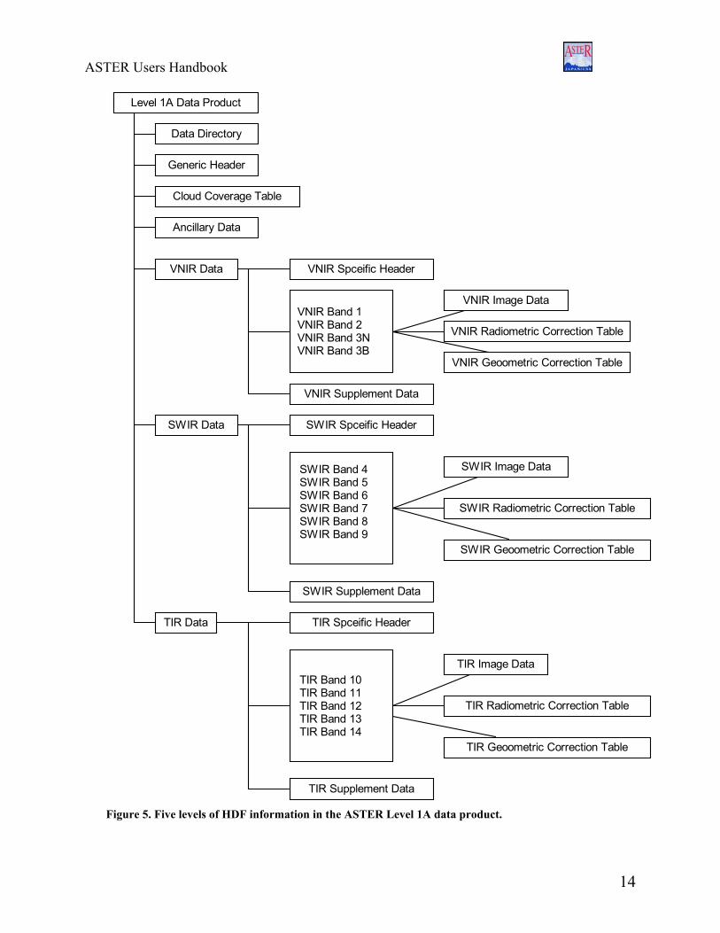
instrument image data with geometric correction coefficients and radiometric calibration coefficients appended but not applied. These coefficients include correcting for SWIR parallax as well as registration between and within telescopes. (The SWIR parallax error is caused by the offset in detector alignment in the along-track direction and depends on the distance between the spacecraft and the observed earth surface. For SWIR bands the parallax corrections are carried out with the image matching technique or the coarse DEM data base, depending on cloud cover.) The spacecraft ancillary and instrument engineering data are also included. The radiometric calibration coefficients, consisting of offset and sensitivity information, are generated from a database for all detectors, and are updated periodically. The geometric correction is the coordinate transformation for band-to-band coregistration. The VNIR and SWIR data are 8-bit and have variable gain settings. The TIR data are 12-bit with a single gain.The structure of the data inside the Level 1A HDF product is illustrated in Figure 5.
13
ASTER Users Handbook
Data Directory
Cloud Coverage Table
Ancillary Data
VNIR Data
Level 1A Data Product
VNIR Spceific Header
VNIR Band 1VNIR Band 2VNIR Band 3NVNIR Band 3B
VNIR Image Data
Generic Header
VNIR Radiometric Correction Table
VNIR Supplement Data
SWIR Data
VNIR Geoometric Correction Table
SWIR Spceific Header
SWIR Band 4SWIR Band 5SWIR Band 6SWIR Band 7SWIR Band 8SWIR Band 9
SWIR Image Data
SWIR Radiometric Correction Table
SWIR Geoometric Correction Table
SWIR Supplement Data
TIR Data TIR Spceific Header
TIR Band 10TIR Band 11TIR Band 12TIR Band 13TIR Band 14
TIR Supplement Data
TIR Image Data
TIR Radiometric Correction Table
TIR Geoometric Correction Table
Figure 5. Five levels of HDF information in the ASTER Level 1A data product.
14

ASTER Users Handbook
3.2 Level 1B Data Product The ASTER Level 1B data are L1A data with the radiometric and geometric coefficients
applied. All of these data are stored together with Metadata in one HDF file. The L1B image is projected onto a rotated map (rotated to “path oriented” coordinate) at full instrument resolutions. The Level 1B data generation also includes registrations of the SWIR and TIR data to the VNIR data. And in addition, for SWIR in particular, the parallax errors due to the spatial locations of all of its bands are corrected. Level 1B data define a scene center as the geodetic center of the scene obtained from the L1A attribute named “SceneCenter” in the HDF-EOS attribute “productmetadata.0”. The definition of scene center in L1B is the actual center on the rotated coordinates (L1B coordinates) not the same as in L1A.
The structure of the L1B data file is shown schematically in Figure 6. This illustration is for the product generated when the instrument is operated in full mode (all systems on and acquiring data). In other restricted modes, e.g. just SWIR and TIR, not all the items listed in Figure 6 are included in the product.
15

ASTER Users Handbook
Data Directory
Ancillary Data
VNIR Data VNIR Spceific Header
VNIR Band 1VNIR Band 2VNIR Band 3NVNIR Band 3B
VNIR Image Data
Generic Header
VNIR Supplement Data
SWIR Data SWIR Spceific Header
SWIR Band 4SWIR Band 5SWIR Band 6SWIR Band 7SWIR Band 8SWIR Band 9
SWIR Image Data
SWIR Supplement Data
TIR Data TIR Spceific Header
TIR Band 10TIR Band 11TIR Band 12TIR Band 13TIR Band 14
TIR Supplement Data
TIR Image Data
Level 1B Data Product
Geolocation Field Data
Figure 6. Five levels of HDF information in the ASTER Level 1B data product.
16

ASTER Users Handbook
The L1B data product is generated for the requested map projection and the resampling method. The defaults are UTM projection in swath orientation, and Cubic Convolution resampling. Other projections and resampling methods are available on request (Table 2).
Table 2. Resampling methods and projections available for producing Level 1B products. Resampling methods Map Projections Nearest Neighbor (NN) Geographic (EQRECT) Cubic Convolution (CC) Lambert Conformal Conic (LAMCC) Bi-Linear (BL) Space Oblique Mercator (SOM) Polar Stereographic (PS) Universal Transverse Mercator (UTM) Each image contains geolocation information stored as a series of arrays. There is one set of
geolocation information (array) per nadir telescope (3 sets total). Each geolocation array is 11 x 11 elements size, with the top left element (0,0) in the image for the nadir views. For the backward view the image is offset with respect to the geolocation array. The nadir VNIR and back-looking VNIR images use the same latitude/longitude array, except the back-looking image is offset with respect to the nadir image.
The L1B latitude and longitude geolocation arrays are two 11 x 11 matrices of geocentric
latitude and geodetic longitude in units of degrees. The block size of the geolocation array is 420 lines by 498 samples for the VNIR bands; 210 lines by 249 samples for the SWIR bands; and 70 lines by 83 samples for the TIR bands.
Appendix I provides a dump of the metadata contained in a L1B data product. There are five metadata groups:
Productmetadata.0 Productmetadata.1 Productmetadata.V Productmetadata.S Productmetadata.T …………….
17

ASTER Users Handbook
4. ASTER Higher-Level Products Table 3 lists each of the ASTER higher-level Standard Data Products and some of their basic
characteristics. More detailed descriptions of these data products are given in Appendix II. Table 3. ASTER higher level standard data products.
Product ID Level Parameter Name Production Mode
Units Absolute Accuracy
Relative Accuracy
Horizontal Resolution
(m)
AST06 2 Decorrelation stretch--VNIR
routine none N/A N/A 15
AST06 2 Decorrelation stretch--SWIR
routine none N/A N/A 30
AST06 2 Decorrelation stretch--TIR
routine none N/A N/A 90
AST04 2 Brightness temperature
on-request
degrees C
1-2 C 0.3 C 90
AST07 2 Surface reflectance
on-request
none 4% 1% 15, 30
AST09 2 Surface radiance--VNIR, SWIR
on-request
W/m2/sr/µm
2% 1% 15, 30
AST09 2 Surface radiance--TIR
on-request
W/m2/sr/µm
2% 1% 90
AST05 2 Surface emissivity
on-request
none 0.05-0.1 0.005 90
AST08 2 Surface kinetic temperature
on-request
degrees K
1-4 K 0.3 K 90
AST13 2 Polar surface and cloud classification
on-request
none 3% 3% 15, 30, 90
AST14 4 Digital elevation model (DEM)
on-request
m >= 7 m >= 10 m 30
18

ASTER Users Handbook
5. Radiometric Parameters
The Level 1B data are in terms of scaled radiance. To convert from DN to radiance at the sensor, the unit conversion coefficients (defined as radiance per 1 DN) are used. Radiance (spectral radiance) is expressed in unit of W/(m2*sr*um). The relation between DN values and radiances is shown below:
(i) a DN value of zero is allocated to dummy pixels (ii) a DN value of 1 is allocated to zero radiance (iii) a DN value of 254 is allocated to the maximum radiance for VNIR and SWIR
bands (iv) a DN value of 4094 is allocated to the maximum radiance for TIR bands (v) a DN value of 255 is allocated to saturated pixels for VNIR and SWIR bands (vi) a DN value of 4095 is allocated to saturated pixels for TIR bands The maximum radiances depend on both the spectral bands and the gain settings and are
shown in Table 4. Table 4. Maximum radiance values for all ASTER bands and all gains.
Maximum radiance (W/(m2*sr*um) Band No. High gain Normal
Gain Low Gain 1 Low gain 2
1 2 3N 3B
170.8 179.0 106.8 106.8
427 358 218 218
569 477 290 290
N/A
4 5 6 7 8 9
27.5 8.8 7.9 7.55 5.27 4.02
55.0 17.6 15.8 15.1 10.55 8.04
73.3 23.4 21.0 20.1 14.06 10.72
73.3 103.5 98.7 83.8 62.0 67.0
10 11 12 13 14
N/A 28.17 27.75 26.97 23.30 21.38
N/A N/A
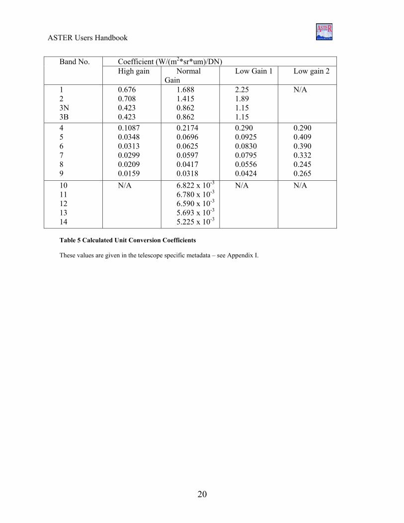
The radiance can be obtained from DN values as follows: Radiance = (DN value – 1) x Unit conversion coefficient
Table 5 shows the unit conversion coefficients of each band
19
ASTER Users Handbook
Coefficient (W/(m2*sr*um)/DN) Band No. High gain Normal
Gain Low Gain 1 Low gain 2
1 2 3N 3B
0.676 0.708 0.423 0.423
1.688 1.415 0.862 0.862
2.25 1.89 1.15 1.15
N/A
4 5 6 7 8 9
0.1087 0.0348 0.0313 0.0299 0.0209 0.0159
0.2174 0.0696 0.0625 0.0597 0.0417 0.0318
0.290 0.0925 0.0830 0.0795 0.0556 0.0424
0.290 0.409 0.390 0.332 0.245 0.265
10 11 12 13 14
N/A 6.822 x 10⁻³ 6.780 x 10⁻³ 6.590 x 10⁻³ 5.693 x 10⁻³ 5.225 x 10⁻³
N/A N/A
Table 5 Calculated Unit Conversion Coefficients These values are given in the telescope specific metadata – see Appendix I.
20

ASTER Users Handbook
6. Data Acquisition
One-time coverage, High sun angle, Optimum gain for the local land surface, Minimum snow and ice cover, Minimum vegetation cover, and No more than 20% cloud cover (perhaps more for special sub-regions).
6.1 Data Acquisition Strategy
Because ASTER does not continuously acquire data, each day’s data takes must be
scheduled and prioritized. The ASTER Science Team has developed a data acquisition strategy to make use of the available resources. Acquisition requests are divided into three categories: local observations, regional monitoring, and global map.
Local Observations: Local Observations are made in response to data acquisition requests from authorized
ASTER Users. Local Observations might include, for example, scenes for analyzing land use, surface energy balance, or local geologic features.
One subset of Local Observations consists of images of such ephemeral events as volcanoes, floods, or fires. Requests for "urgent observations" of such phenomena must be fulfilled in short time periods (of a few days). These requests receive special handling.
Regional Monitoring Data: Regional data sets contain the data necessary for analysis of a large region (often many
regions scattered around the Earth) or a region requiring multi-temporal analysis. A "Local Observation" data set and a "Regional Monitoring" data set are distinguished by the amount of viewing resources required to satisfy the request, where smaller requirements are defined as Local Observations and larger requirements are defined as Regional Monitoring.
The ASTER Science Team has already selected a number of Regional Monitoring tasks. Among the most significant are three that involve repetitive imaging of a class of surface targets:
1. The world's mountain glaciers, 2. The world's active and dormant volcanoes, and 3. The Long-Term Ecological Research (LTER) field sites. Global Map: The Global data set will be used by investigators of every discipline to support their research.
The high spatial resolution of the ASTER Global Map will complement lower resolution data acquired more frequently by other EOS instruments. This data set will include images of the entire Earth’s land surface, in all ASTER spectral bands and stereo.
Each region of the Earth has been prioritized by the ASTER Science Team for observation as part of the Global Map.
Currently the following characteristics have been identified for images in the Global Map data set:
21

ASTER Users Handbook
Allocation of science data: At the present time, it is expected that approximately 25% of ASTER resources will be
allocated to Local Observations, 50% to Regional Monitoring, and 25% to the Global Map. Global Map data has been further sub-divided among high priority areas which are currently
allocated 25%, medium priority areas which are currently allocated 50%, and low priority areas which are currently allocated 25%.
Regional Monitoring data sets and the Global Map will be acquired by ASTER, in response to acquisition requests submitted by the ASTER Science Team acting on behalf of the science community. These Science Team Acquisition Requests (STARs) are submitted directly to the ASTER Ground Data System in Japan. Under limited circumstances, STARs for Local Observations may also be submitted by the Science Team.
STARs for Regional Monitoring data are submitted by the ASTER Science Team only after a proposal for the Regional Monitoring task has been submitted and accepted. These "STAR Proposals" will be evaluated by ASTER's science working groups before being formally submitted to the Science Team.
An already-authorized ASTER User, who wants ASTER to acquire far more data than he or she is allocated, may submit a STAR Proposal to the Science Team. Please note that the process for evaluating STAR proposals is cumbersome and time-consuming. Far fewer STAR Proposals will be approved than ASTER User Authorization Proposals.
6.2 Search and Order Data Products The EOSDIS at the EDC DAAC archives and distributes ASTER Level 1A, Level 1B,
and Decorrelation Stretch products, and also produces on-demand higher level data products.
22
ASTER Users Handbook
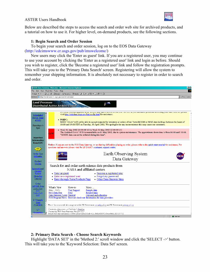
Below are described the steps to access the search and order web site for archived products, and a tutorial on how to use it. For higher level, on-demand products, see the following sections.
1: Begin Search and Order Session To begin your search and order session, log on to the EOS Data Gateway
(http://edcimswww.cr.usgs.gov/pub/imswelcome/) New users may click the 'Enter as guest' link. If you are a registered user, you may continue
to use your account by clicking the 'Enter as a registered user' link and login as before. Should you wish to register, click the 'Become a registered user' link and follow the registration prompts. This will take you to the 'Primary Data Search' screen. Registering will allow the system to remember your shipping information. It is absolutely not necessary to register in order to search and order.
2: Primary Data Search - Choose Search Keywords Highlight 'DATA SET' in the 'Method 2:' scroll window and click the 'SELECT ->' button.
This will take you to the 'Keyword Selection: Data Set' screen.
23

ASTER Users Handbook
A list of data sets available are displayed in the 'Data Set list 1' scroll window. Highlight the data set or sets you wish to search and click 'OK!'.
Normally, you should select “ASTER L1A reconstructed unprocessed instrument data V002
& V003”; and “ASTER L1B registered radiance at the sensor V002 & V003”. The other choice of expedited data are scenes that were processed in expedited mode, and are only temporary in the archive; they are replaced as soon as the standard processed product arrives from Japan.
3: Primary Data Search - Choose Search Area You may now enter your area-of-interest. 'Type in Lat/Lon Range' will be the default method to define your search area. If you know
the Latitude and Longitude, enter the coordinates.
24

ASTER Users Handbook
To define the geographic area on a map, click the radio button next to your map of choice and select the region by clicking on the map.
4: (optional): Primary Data Search - Choose a Time Range (not required) You may now enter your Date or Time Range. You may use either a Standard Date Range or
Julian Date Range. Be sure to enter the date and time by following the format provided. To search seasonally, select the radio button next to 'Annually Repeating'.
5: Primary Data Search - Start Search!
You are now ready to execute your search. Click the 'Start Search!' button to begin. 6: Results: Data Set Listing
25
ASTER Users Handbook
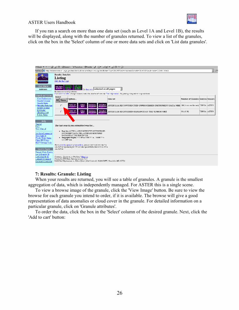
If you ran a search on more than one data set (such as Level 1A and Level 1B), the results will be displayed, along with the number of granules returned. To view a list of the granules, click on the box in the 'Select' column of one or more data sets and click on 'List data granules'.
7: Results: Granule: Listing When your results are returned, you will see a table of granules. A granule is the smallest
aggregation of data, which is independently managed. For ASTER this is a single scene. To view a browse image of the granule, click the 'View Image' button. Be sure to view the
browse for each granule you intend to order, if it is available. The browse will give a good representation of data anomalies or cloud cover in the granule. For detailed information on a particular granule, click on 'Granule attributes'.
To order the data, click the box in the 'Select' column of the desired granule. Next, click the 'Add to cart' button:
26

ASTER Users Handbook
8: Shopping Cart - Step 1: Choose Ordering Options Click the 'Order options' button and choose your output media. You will have the option to
apply the output media and processing parameters to all granules or to just one granule. Click the 'Ok! Accept my choice & return to the shopping cart' button to proceed.
You will want to repeat this for each remaining granule if you are ordering data from more than one data set, or if you did not apply the ordering options to all granules.
When finished with your processing parameters, click the 'Go to Step 2: Order Form' button.
27

ASTER Users Handbook
9: Shopping Cart: - Step 2: Order Form Enter your appropriate address in the contact, shipping and billing address fields. You are
required to enter text in the red fields. If you are a registered user, this page will be completed for you. When finished, choose your affiliation and click the 'Go to Step 3: Review Order Summary' button.
28

ASTER Users Handbook
10: Shopping Cart: - Step 3: Order Summary Review the order summary. If all of the information is correct, click the 'Go to Step 4:
Submit Order!' button. 11: Order Submitted Your order has now been submitted. You will receive automatic email(s) confirming the
receipt of your order. The EDC email will summarize your order, cost, and provide information on Modes of Payment. Payment must be received before order processing can begin. Please contact EDC to arrange payment and include your order number on all modes of payment.
29

ASTER Users Handbook
6.3. Ordering Level 2 Products Digital Elevation Model (DEM) From the Level 1A granules search page, you will see a link next to the granule listing
that takes you to the DEM order page. Follow the instructions there to order a relative or absolute DEM. Note that for a relative DEM, you have only to cut and paste the L1A scene ID into the appropriate place, and submit the order. For an absolute DEM, you must provide Ground Control Points. To accomplish this, you must first order the L1A data, locate your GCP’s on both the 3N and 3B images, and supply these pixel coordinates along with the GCP coordinate locations.
Level 2 Products except DEM From the Level 1B granules search page, you will see a link next to the granule listing
that takes you to the higher level data products order pages. The site allows you to select a product (such as reflectance), and then allows you to customize the processing (or accept the default parameters).
6.4 Data Acquisition Requests
Data Acquisition Requests (DARs) are user requests to have ASTER acquire new data
over a particular site at specified times. If the desired ASTER observations have not yet been acquired or even requested, a requestor can become an authorized ASTER User, and can then submit a data acquisition request (DAR) via the DAR Tool. To register as an authorized ASTER User, use the link below which will take you to the web site for registering, and explains the procedure:
http://asterweb.jpl.nasa.gov/gettingdata/authorization/default.htm Once you are registered, you can go to the on-line ASTER DAR Tool web site to enter
your request: http://e0ins02u.ecs.nasa.gov:10400/ Be sure to read the “Getting Started” information for help on using the tool, and getting any
plug-ins necessary.
7. Application Examples
7.1 Cuprite, Nevada
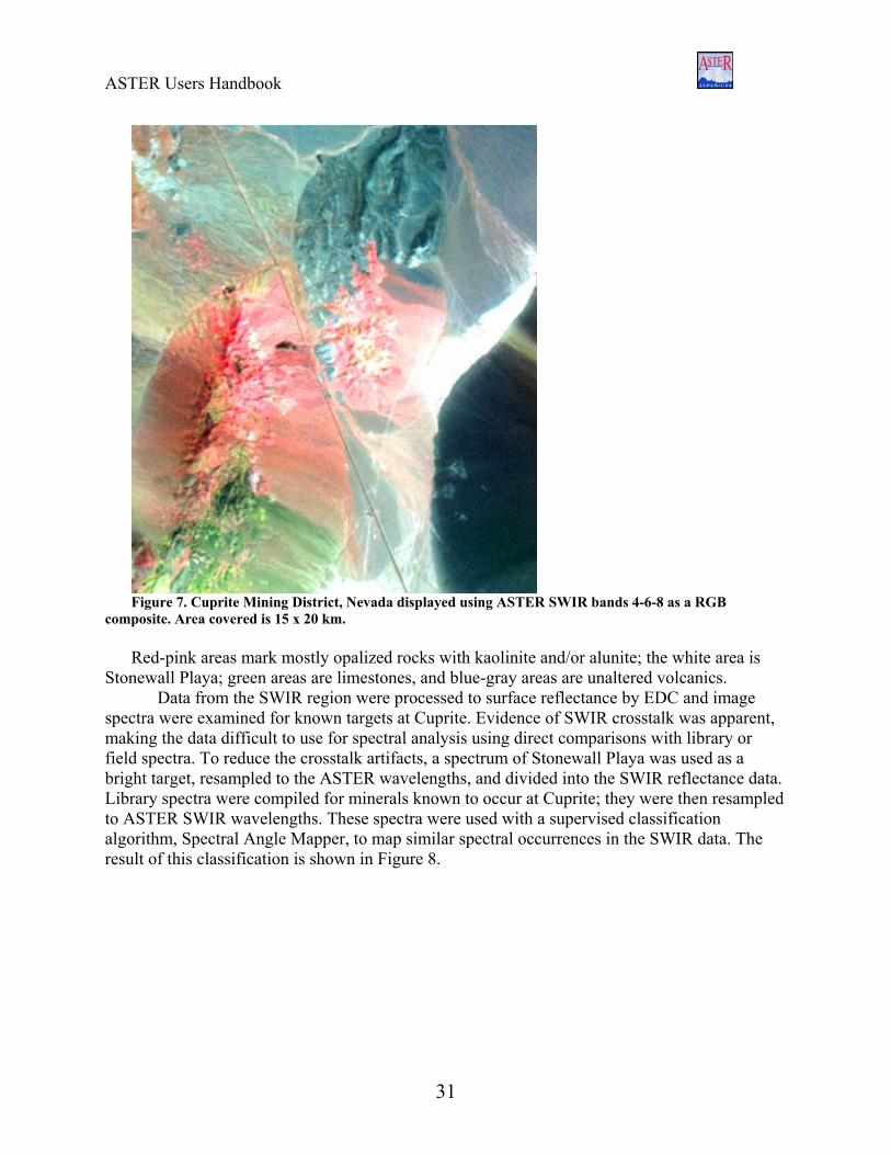
The Cuprite Mining District is located in west-central Nevada, and is one of a number of alteration centers explored for precious metals. Cambrian sedimentary rocks and Cenozoic volcanic rocks were hydrothermally altered by acid-sulfate solutions at shallow depth in the Miocene, forming three mappable alteration assemblages: 1) silicified rocks containing quartz and minor alunite and kaolinite; 2) opalized rocks containing opal, alunite and kaolinite; 3) argillized rocks containing kaolinite and hematite. A general picture of the alteration is shown in Figure 1, combining bands 4,6 and 8 in RGB and processed to increase the color saturation.
30
ASTER Users Handbook
Figure 7. Cuprite Mining District, Nevada displayed using ASTER SWIR bands 4-6-8 as a RGB
composite. Area covered is 15 x 20 km. Red-pink areas mark mostly opalized rocks with kaolinite and/or alunite; the white area is
Stonewall Playa; green areas are limestones, and blue-gray areas are unaltered volcanics. Data from the SWIR region were processed to surface reflectance by EDC and image
spectra were examined for known targets at Cuprite. Evidence of SWIR crosstalk was apparent, making the data difficult to use for spectral analysis using direct comparisons with library or field spectra. To reduce the crosstalk artifacts, a spectrum of Stonewall Playa was used as a bright target, resampled to the ASTER wavelengths, and divided into the SWIR reflectance data. Library spectra were compiled for minerals known to occur at Cuprite; they were then resampled to ASTER SWIR wavelengths. These spectra were used with a supervised classification algorithm, Spectral Angle Mapper, to map similar spectral occurrences in the SWIR data. The result of this classification is shown in Figure 8.
31

ASTER Users Handbook
Figure 8. Spectral Angle Mapper classification of Cuprite SWIR data. blue=kaolinite; red=alunite;
light green=calcite; dark green=alunite+kaolinite; cyan=montmorillonite; purple=unaltered; yellow=silica or dickite.
When this map was compared with more detailed mineral classification produced from AVIRIS data, the correspondence is excellent. The resampled library spectra are shown in Figure 9 compared with ASTER image spectra extracted from 3x3 pixel areas.
32

ASTER Users Handbook
Figure 9. ASTER image spectra (left) and library spectra(right) for minerals mapped at Cuprite.
33

ASTER Users Handbook
7.2 Lake Tahoe
Objective The objective of the Lake Tahoe CA/NV case study is to illustrate the use of ASTER data for water-related studies. Introduction Lake Tahoe is a large lake situated in a granite graben near the crest of the Sierra Nevada Mountains on the California - Nevada border, at 39° N, 120° W. The lake level is approximately 1898 m above MSL. The lake is roughly oval in shape with a N-S major axis (33 km long, 18 km wide), and has a surface area of 500 km2 (Figure 10).
Figure 10. Outline map of Lake Taoe CA/NV
The land portion of the watershed has an area of 800 km2. Lake Tahoe is considered a deep lake, it is the 11th deepest lake in the world, with an average depth of 330 m, maximum depth of 499 m, and a total volume of 156 km3. The surface layer of Lake Tahoe deepens during the fall and winter. Complete vertical mixing only occurs every few years. Due to its large thermal mass, Lake Tahoe does not freeze in winter. There are approximately 63 streams flowing into
34

ASTER Users Handbook
the lake and only one river flowing out of the lake. Lake Tahoe is renowned for its high water clarity. However, the water clarity has been steadily declining from a maximum secchi depth of 35 m in the sixties to its current value of ~20 m. Research by UC Davis has identified that the decline is in part due to increased algal growth facilitated by an increase in the amount of nitrogen and phosphorus entering the lake and, in part, due to accumulation of small suspended inorganic particulates derived from accelerated basin-wide erosion and atmospheric inputs. Field Measurements In order to validate the data from the MODIS and ASTER instruments, the Jet Propulsion Laboratory (JPL) and UC Davis (UCD) are currently maintaining four surface sampling stations on Lake Tahoe (Hook et al. 2002). The four stations (rafts/buoys) are referred to as TR1, TR2, TR3 and TR4 (Figure 10). Each raft/buoy has a single custom-built self-calibrating radiometer for measuring the skin temperature and several bulk temperature sensors. The radiometer is mounted on a pole approximately 1m above the surface of the water that extends beyond the raft (Figure 11).
Figure 11. Raft measurementss.
The radiometer is orientated such that it measures the skin temperature of the water directly beneath it. The radiometer is contained in a single box that is 13 cm wide 43 cm long and 23 cm high (Figure 11). The sensor used in the radiometer is a thermopile detector with a germanium lens embedded in a copper thermal reservoir. The sensor passes radiation with wavelengths between 7.8 and 13.6 µm. The unit is completely self-contained and has an on-board computer and memory and operates autonomously. The unit can store data on-board for later download or
35

ASTER Users Handbook
automatically transmit data to an external data logger. The unit can be powered for short periods (several hours) with its internal battery or be powered for longer periods with external power. In this study the radiometer is powered externally and data are transferred to an external data logger. The radiometer uses a cone blackbody in a near-nulling mode for calibration and has an accuracy of ± 0.1 K. The accuracy of the radiometers was confirmed in a recent cross comparison experiment with several other highly accurate radiometers in both a sea trial and in laboratory comparisons. It should be noted the current design of both the radiometers does not include a sky view and therefore the correction for the reflected sky radiation is made using a radiative transfer model (MODTRAN). The bulk water temperature is measured with several temperature sensors mounted on a float tethered behind the raft/buoy (Figure 11). The float was built in the shape of a letter H and is 203 cm long and 70 cm wide. At the end of each point of the letter H is a short leg at right angles to the float and the temperature sensors are attached to the end of the leg approximately 2cm beneath the surface. Multiple temperature sensors are used to enable cross verification and each float has up to 12 temperature sensors all at the same depth. The temperature sensors used include the Optic Stowaway and Hobo Pro Temperature Loggers available from Onset Corporation (www.onsetcomp.com) and a TempLine system available from Apprise Technologies (www.apprisetech.com). The Optic Stowaway Temperature Loggers include both the sensor and data logger in a single sealed unit with a manufacturer specified maximum error of ± 0.25 °C. The Hobo Pro Temp/External Temperature logger has an external temperature sensor at the end of a short cable that returns data to a logger and a manufacturer specified maximum error of ± 0.2 °C. The TempLine system consists of 4 temperature sensors embedded at different positions along a cable that is attached to a data logger. The TempLine system has a manufacturer specified error of ± 0.1° C. Note all sensors are placed at the same depth ensuring both redundancy and cross verification. The calibration accuracy of the Onset temperature sensors was checked using a NIST traceable water bath. NIST traceability was provided by use of a NIST certified reference thermometer. In all cases the sensors were found to meet the manufacturer specified typical error of ± 0.12 C. Data collected by the external data logger (radiometer and TempLine system) can be downloaded automatically via cellular telephone. Currently the external data logger data are downloaded daily via cellular telephone modem to JPL allowing near real-time monitoring. A full set of measurements is made every 2 minutes. However, the units attached to the external data logger can be remotely re-programmed if a different sampling interval is desired. The initial rafts are currently being replaced by buoys as pictured above which also include a meteorological station providing wind speed, wind direction, air temperature, relative humidity and net radiation (Figure 11). Additional UCD atmospheric deposition collectors are located on TR2 and TR3. Both JPL and UCD maintain additional equipment at the US Coast Guard station that provides atmospheric information (Figure 12). This includes a full meteorological station (wind speed, wind direction, air temperature, relative humidity), full radiation station (long and shortwave radiation up and down), a shadow band radiometer and an all sky camera. The shadow band radiometer provides information on total water vapor and aerosol optical depth.
36

ASTER Users Handbook
Figure 12. Field measurements at the USCG.
Measurements of algal growth rate using 14C, nutrients (N, P), chlorophyll, phytoplankton, zooplankton, light, temperature and secchi disk transparency are also made tri-monthly at the Index station (Figure 10) and monthly samples for all constituents except algal growth and light are made at the Mid-lake station (Figure 10). Many samples are taken annually around the Tahoe Basin to examine stream chemistry and snow and atmospheric deposition constituents. Using ASTER to measure water clarity Currently the decline in water clarity at Lake Tahoe is measured using a secchi disk – a white disk that is lowered into the water until it is no longer visible. The UC Davis Tahoe Research Group have been making secchi disk measurements since the mid 60’s at two locations on the lake (Midlake and Index – see Figure 10). Such measurements have been used to monitor the decline in clarity from a maximum of 35 m when measurements began to the current low of 20 m. These measurements are crucial for monitoring temporal changes in clarity but provide little information on spatial variations in clarity across and around the lake. Knowledge of spatial variations in clarity could prove useful in identifying areas of high nutrient or sediment input into the lake.
37

ASTER Users Handbook
Examination of a color infrared composite image derived from ASTER for Lake Tahoe (Figure 13) indicates that due to the high clarity the bottom of the lake is visible for some distance from the shore.
Figure 13. Color Infrared Composite of ASTER bands 3,2,1 as R,G,B respectively. Red areas indicate vegetation, white areas are snow.
Places where the bottom of the lake is visible appear dark blue, for example the southern margin of the lake. The bottom is can be seen for the greatest distance from the shore in ASTER band 1 and this band can be color coded to show variations in the intensity of the bottom reflectance (Figure 14).
38

ASTER Users Handbook
Figure 14. ASTER band 1 (0.52-0.60um) color coded to show variations in the intensity of the near-shore bottom reflectance.
In this image, areas where the bottom is visible are colored red and green (greater bottom reflectance is shown in red). Where the lake is blue the bottom cannot be seen. The depth to which the bottom is visible varies depending on the clarity of the water. In order to investigate this further an accurate bathymetric map was registered to the ASTER data. The accuracy of the bathymetric map is ~0.5 % of the waterdepth. The bathymetric map is shown in Figure 15 color coded with greater depths shown in blue and shallower depths shown in red.
39

ASTER Users Handbook
Figure 15. Bathymetric map of Lake Tahoe CA/NV.
Once the bathymetric map is registered to the ASTER image the depth at which the bottom is no longer visible can be determined and can be used to produce a near shore clarity map shown in Figure 16.
plit-window algorithm. In the split-window algorithm the at-sensor radiances are regressed can then be used to
correct other datasets without ground measurements. Alternatively a physics-based approach can
Figure 16. Near-shore clarity map derived from ASTER data and a bathymetric map.
Examination of Figure 16 indicates some places where the lake is exceptionally clear and other areas where it is less so. For example the areas in the southwest and northeast are particularly clear whereas the area in the southeast is less clear. There is little sediment input in the southwest and northeast whereas the Upper Truckee River flows in from the south and strongly affects the southeast. Further work is underway to validate the accuracy of this map and look for seasonal changes in clarity as well as changes over time. Using ASTER to measure circulation In addition to making measurements in the reflected infrared, the ASTER instrument also measures the radiation emitted in the thermal infrared part of the spectrum. These data can be used to measure the surface temperature and produce maps of lake surface temperature. Such maps are valuable for the understanding of a variety of processes in lakes, such as wind-induced upwelling events and surface water transport patterns. In order to derive the surface temperature it is necessary to correct the data for atmospheric effects. Two approaches are commonly used to correct the data. The most common approach is a sagainst simultaneous ground measurements to derive a set of coefficients that
40

ASTER Users Handbook
be used which couples a surface temperature and emissivity model with a radiative transfer model. The ASTER team has developed a physics based approach for extracting temperature aemissivity and a user can order either a surface temperature (AST08) or surface emissivity (AST05) product. The image below shows an at-sensor brightness
nd
temperature image for Lake Tahoe from ASTER ata acquired at night on June 3rd 2001. Examination of the image indicates a strong cold plume
across the lake to the east shore, then spreading north nd south. The cold plume of water is the result of a wind-induced upwelling event in west. The
e
und the lake.
dof water originating in the west, travelingaupwelling is induced by strong, persistent winds from the southwest which move the surfacwater to the east allowing the deep cold water in the west to upwell. The cold water is nutrient rich compared with the warmer surface waters which have been depleted of nutrients. The temperature images from ASTER can be used to map these nutrient pathways which help explainthe distribution of organic matter and fine sediments aro
41

ASTER Users Handbook
Figure 17. ASTER band 13 brightness temperature image of Lake Tahoe acquired June 3, 2001.
42

ASTER Users Handbook
8. Frequently asked questions
ASTER Instrument What are sizes of ASTER pixels? ASTER provides data at 3 different spatial resolutions (pixel sizes). The resolutions are 15 m, 30 m and 90 m for the visible-near infrared, shortwave infrared and thermal infrared respectively. For more information check the ASTER web page (http://asterweb.jpl.nasa.gov) Where do I find information about the ASTER instrument characteristics, e.g. the signal to noise? The ASTER instrument characteristics including the signal to noise are given on the ASTER webpage under instrument.
Acquiring and Ordering ASTER Data How do I find out if ASTER data are available over my study area and if they are not how do I get them acquired? To find out if ASTER data are available search the ASTER archives via the Eros Data Center Gateway (EDG) all acquired data are archived and distributed there (http://edcimswww.cr.usgs.gov/pub/imswelcome/). You may enter as Guest for search purposes. There will also be information for ordering data. If your Area of Interest has not been collected, you may submit a Data Acquisition Request proposal for evaluation. Once approved the user is granted privileges for submitting a limited number of observation requests. These requests go directly into the scheduling database. The following url will direct you to the DARtool users request form. http://asterweb.jpl.nasa.gov/gettingdata/authorization/default.htm . Read through the short three page directions and proceed to enter your proposal request. Further instructions will follow once the proposal has been submitted for evaluation. How much do ASTER data cost? Currently ASTER Level 1A and 1B data are available from the EDC DAAC at $55 per scene. Higher level data products are free. (http://edcimswww.cr.usgs.gov/pub/imswelcome/). How do I find out when ASTER will be over my site? There is a web based tool available at: http://earthobservatory.nasa.gov/MissionControl/overpass.html that can be used for overpass predictions. Using the tool: The Spacecraft designation should be “TERRA”. Enter the overpass criteria then execute the prediction using the predict button. On the results page, look at the Peak time (utc) for the given date with Peak Elevation angles greater than 81.5 deg. and with “Vis” field ‘DDD’ for Day scenes and ‘ NNN’ for night scenes. If the Peak Elevation is less than 81.5 deg, the target is NOT in the instruments field of view for that overpass on that day. ASTER can acquire data from the VNIR telescope more frequently by pointing. Are ASTER data acquired over every location every 16 days. No, although ASTER can acquire data over the same location every 16 days its limited duty
43

ASTER Users Handbook
cycle prevents it from acquiring all locations every 16 days. If you want data for a particular overpass then you should get in touch with the ASTER team to find out how to submit a request to make sure the instrument is turned on over your site on that particular 16 day cycle. The ASTER Science Support Scheduling group (SSSG) can be contacted via the ASTER web site: http://asterweb.jpl.nasa.gov Does the EDC Catalogue contain all the ASTER scenes? Yes the EDC catalogue contains all the ASTER scenes, searching on Level 1A data searches all ASTER data acquired. It typically takes 4-6 weeks after acquisition for a scene to reach the DAAC. Can I order a mosaic of several ASTER scenes? No ASTER data are only available as single scenes. I submitted a proposal to have ASTER data acquired over my area. What happens next? When a proposal is submitted, there is an automated confirmation response sent from the server database. If you do not receive the email notification you will need to resubmit the proposal again. After proper acceptance into the database, it has been taking eight to twelve weeks for complete evaluation and processing. We are actively working towards reducing the cycle time response to less than six weeks. We do appreciate everyone’s patience during this transition. I submitted a Data Acquisition Request (DAR) to have ASTER acquire data over my site. Where do I go to find out whether the DAR was successful? The DARtool is capable of acquisition status but does not include any cloud cover ratings. If the status of a DAR is said to have ‘failed’ it generally means that there was no acquisition made before the LifeTime of the DAR expired. Acquisitions are determined by very complex scheduling algorithms. Delivery of the acquired data sets is usually between three and four weeks after acquisition. On occasion, the process can be completed within two weeks of an acquisition but may require special operator handling.
Processing and Products Where do I find out more about the algorithms used to process ASTER data? The algorithms used to process ASTER data are described in the ASTER Theoretical Basis Documents (ATBD’s). These can be downloaded from the ASTER web site. The ASTER 1A data contain both geometric (e.g. band offsets) and radiometric artifacts (e.g. striping) is there any software I can get to remove these? ASTER 1A data are the raw data with the radiometric and geometric correction coefficients appended but not applied. They are applied in the 1B product. You should order the 1B product. The software for processing the 1A to 1B data only runs at the DAAC. Are ASTER 1b images radiometrically calibrated? Yes, ASTER 1b images are radiometrically calibrated, however, in order to keep image sizes small they are rescaled in the byte and halfword ranges (the VNIR and SWIR are in byte) and the TIR are in halfword (2 byte). In order to scale the data to the correct range you need to apply the
44

ASTER Users Handbook
coefficients listed earlier in this document. Are ASTER 1b images always processed to the same version? No there have been multiple updates to the software and if you downloaded the ASTER data over your site a few months ago there may now be a new version of the same scene. You should always try and get the latest version since each new version improves the data, e.g. the registration between bands. This is because our understanding of how the instrument behaves in space has improved over time. You get the latest version by ordering the data from the most recent collection for a given product at the DAAC. In some cases only an older version may be available. Are there any tools available for converting ASTER data into other formats, e.g. GeoTIFF so I can use them in other packages e.g. IDL/ENVI, Arc/Info, ERDAS/Imagine? The latest version of ENVI allows you to read ASTER data. The ASTER team has developed free tools for processing ASTER data. They are available from: http://winvicar.jpl.nasa.gov/ Where can I find the latitude/longitude of the corner points of my ASTER scene? The corner points of a given ASTER scene are provided in the metadata inside the HDF file. They are also given in the .met file, an ascii text file that comes with the HDF file. How do I find the latitude and longitude of an ASTER pixel? The 1B file contains latitude/longitude arrays for each of the 3 instruments (VNIR, SWIR, TIR) which can be expanded to obtain the latitude/longitude of every pixel. Note the latitude values of the 1B data are in geocentric coordinates whereas the longitude values are in geodetic coordinates. You need to convert the geocentric to geodetic coordinates. For further details see the section on geometric conversion in this document. ASTER scenes are rotated (not N-S) where do I find the amount of rotation? The amount of rotation is given in the HDF file. It should also be noted that the latitude in the Level 1B product is in geocentric cords whereas the longitude is in geodectic coords. Please consult the section in this guide on ASTER geometry for further details. How do I get a DEM generated from ASTER data for my area? ASTER DEM’s can be produced as an on-demand product through the EDG website. You must first search for Level 1A data, then follow the link next to the granule ID. Please note that our production rate is 1-2 DEM’s per day, so there is a queue of several months. Are the DEM’s absolute or relative? Both absolute and relative DEM’s can be ordered. For absolute DEM’s you need to provide a control point. How do I get the surface reflectance from the ASTER 1b data? The ASTER team provides a reflectance product that can be ordered when the 1B data are ordered. However, there are problems with crosstalk from band 5 to band 9. The problem is under investigation.
45

ASTER Users Handbook
How do I get temperature and emissivity from ASTER 1b data? The ASTER team provides a temperature and emissivity product that can be ordered when the 1B data are ordered.
46

ASTER Users Handbook
9. Software Availability
All EOS data products are stored in Hierarchical Data Format (HDF). This format is very
flexible and accommodates the wide range of products available from the EOS instruments. Although HDF is a flexible storage format, it can be a daunting task getting data out of HDF and into a users image analysis and display package. Fortunately several image analysis and display packages are able to ingest ASTER data making it easy for users that have those packages to begin working with the data. Users are cautioned that some of these packages do not always ingest the files correctly and care should be taken to check the file has been ingested correctly. There are also other programs that allow uses to search the metadata associated with a product. The EOS project maintains a list of software packages that are able to work with EOS data at:
http://hdfeos.gsfc.nasa.gov/hdfeos/viewingHDFEOS.html In addition to these packages JPL also have an image analysis package (WINVICAR) that
works under Windows NT, 2000 and XP. This package includes programs for getting ASTER data out of HDF and into ASCII, BINARY and WINVICAR format. There are also programs to dump the metadata from ASTER data files. For more information please visit:
http://winvicar.jpl.nasa.gov
47

ASTER Users Handbook
Appendix I. Dump of HDF metadata in L1B file coremetadata.0 SHORTNAME= "ASTL1B" SIZEMBDATAGRANULE= 119.185000 PRODUCTIONDATETIME= "2001-04-14T07:24:17.000Z" PLATFORMSHORTNAME= "AM-1" INSTRUMENTSHORTNAME= "ASTER" WESTBOUNDINGCOORDINATE= 29.260599 NORTHBOUNDINGCOORDINATE= -4.082604 EASTBOUNDINGCOORDINATE= 30.006667 SOUTHBOUNDINGCOORDINATE= -4.741722 TIMEOFDAY= "084727306000Z" CALENDARDATE= "20000717" FUTUREREVIEWDATE= "20001225" SCIENCEREVIEWDATE= "20001109" QAPERCENTMISSINGDATA= 0.001309 QAPERCENTOUTOFBOUNDSDATA= 0.001309 QAPERCENTINTERPOLATEDDATA= 0.000000 REPROCESSINGACTUAL= "not reprocessed" PGEVERSION= "03.00R02" PROCESSINGLEVELID= "1B" MAPPROJECTIONNAME= "Universal Transverse Mercator" productmetadata.0 IDOFASTERGDSDATAGRANULE= "ASTL1B 0007170847270104141228" RECEIVINGCENTER= "EDOS" PROCESSINGCENTER= "ASTER-GDS" SENSORNAME= "VNIR" POINTINGANGLE= 8.578000 SETTINGTIMEOFPOINTING= "2000-07-17T08:41:54Z" SENSORNAME= "SWIR" POINTINGANGLE= 8.547000 SETTINGTIMEOFPOINTING= "2000-07-17T08:41:53Z" SENSORNAME= "TIR" POINTINGANGLE= 8.567000 SETTINGTIMEOFPOINTING= "2000-07-17T08:41:53Z" GAIN= ("01", "HGH") GAIN= ("02", "HGH") GAIN= ("3N", "NOR") GAIN= ("3B", "NOR") GAIN= ("04", "NOR") GAIN= ("05", "NOR") GAIN= ("06", "NOR") GAIN= ("07", "NOR") GAIN= ("08", "NOR") GAIN= ("09", "NOR") GEOMETRICDBVERSION= ("01.02", "2000-10-25") RADIOMETRICDBVERSION= ("01.02", "2000-11-09") COARSEDEMVERSION= ("1.00", "1997-09-03", "This data is generated from
GTOPO30") SCENECLOUDCOVERAGE= 7 QUADRANTCLOUDCOVERAGE= (4, 13, 1, 11) SOURCEDATAPRODUCT= ("ASTL1A 0007170847270103051199", "2001-03-
05T15:23:38.000Z", "PDS") ASTEROPERATIONMODE= "OBSERVATION"
48

ASTER Users Handbook ASTEROBSERVATIONMODE= ("VNIR1", "ON") ASTEROBSERVATIONMODE= ("VNIR2", "ON") ASTEROBSERVATIONMODE= ("SWIR", "ON") ASTEROBSERVATIONMODE= ("TIR", "ON") PROCESSEDBANDS= "01023N3B0405060708091011121314" ASTERSCENEID= (173, 176, 7) ORBITNUMBER= 3087 RECURRENTCYCLENUMBER= (14, 58) FLYINGDIRECTION= "DE" SOLARDIRECTION= (37.043010, 57.701316) SPATIALRESOLUTION= (15, 30, 90) UPPERLEFT= (-4.082604, 29.341137) UPPERRIGHT= (-4.178226, 30.006667) LOWERLEFT= (-4.646324, 29.260599) LOWERRIGHT= (-4.741722, 29.926708) SCENECENTER= (-4.412223, 29.633727) SCENEORIENTATIONANGLE= -8.336200 productmetadata.1 SENSORSHORTNAME= ("ASTER_VNIR", "ASTER_SWIR", "ASTER_TIR") IDOFASTERGDSDATABROWSE= "ASTL1A 0007170847270103051199B" productmetadata.v IMAGEDATAINFORMATION1= (4980, 4200, 1) MINANDMAX1= (42, 255) MEANANDSTD1= (60.425335, 6.740928) MODEANDMEDIAN1= (54, 148) NUMBEROFBADPIXELS1= (0, 0) CORINTEL1= "N/A" CORPARA1= "N/A" RESMETHOD1= "CC" MPMETHOD1= "UTM" PROJECTIONPARAMETERS1= (6378137.000000, 6356752.300000, 0.999600,
0.000000, 0.471239, 0.000000, 500000.000000, 0.000000, 0.000000, 0.000000, 0.000000, 0.000000, 0.000000)
UTMZONECODE1= 35 INCL1= 0.676000 OFFSET1= -0.676000 CONUNIT1= "W/m2/sr/um" IMAGEDATAINFORMATION2= (4980, 4200, 1) MINANDMAX2= (25, 251) MEANANDSTD2= (42.124893, 12.541837) MODEANDMEDIAN2= (29, 138) NUMBEROFBADPIXELS2= (0, 0) CORINTEL2= "N/A" CORPARA2= "N/A" RESMETHOD2= "CC" MPMETHOD2= "UTM" PROJECTIONPARAMETERS2= (6378137.000000, 6356752.300000, 0.999600,
0.000000, 0.471239, 0.000000, 500000.000000, 0.000000, 0.000000, 0.000000, 0.000000, 0.000000, 0.000000)
UTMZONECODE2= 35 INCL2= 0.708000 OFFSET2= -0.708000 CONUNIT2= "W/m2/sr/um" IMAGEDATAINFORMATION3N= (4980, 4200, 1)
49
ASTER Users Handbook MINANDMAX3N= (13, 209) MEANANDSTD3N= (40.284557, 21.741985) MODEANDMEDIAN3N= (17, 111) NUMBEROFBADPIXELS3N= (0, 0) CORINTEL3N= "N/A" CORPARA3N= "N/A" RESMETHOD3N= "CC" MPMETHOD3N= "UTM" PROJECTIONPARAMETERS3N= (6378137.000000, 6356752.300000, 0.999600,
0.000000, 0.471239, 0.000000, 500000.000000, 0.000000, 0.000000, 0.000000, 0.000000, 0.000000, 0.000000)
UTMZONECODE3N= 35 INCL3N= 0.862000 OFFSET3N= -0.862000 CONUNIT3N= "W/m2/sr/um" IMAGEDATAINFORMATION3B= (4980, 4600, 1) MINANDMAX3B= (20, 255) MEANANDSTD3B= (60.560661, 15.758011) MODEANDMEDIAN3B= (55, 137) NUMBEROFBADPIXELS3B= (0, 0) CORINTEL3B= "N/A" CORPARA3B= "N/A" RESMETHOD3B= "CC" MPMETHOD3B= "UTM" PROJECTIONPARAMETERS3B= (6378137.000000, 6356752.300000, 0.999600,
0.000000, 0.471239, 0.000000, 500000.000000, 0.000000, 0.000000, 0.000000, 0.000000, 0.000000, 0.000000)
UTMZONECODE3B= 35 INCL3B= 0.862000 OFFSET3B= -0.862000 CONUNIT3B= "W/m2/sr/um" productmetadata.s IMAGEDATAINFORMATION4= (2490, 2100, 1) MINANDMAX4= (1, 255) MEANANDSTD4= (35.554417, 25.348192) MODEANDMEDIAN4= (9, 128) NUMBEROFBADPIXELS4= (0, 0) PROCESSINGFLAG4= 1 NUMBEROFMEASUREMENTS4= 266 MEASUREMENTPOINTNUMBER4= 224 AVERAGEOFFSET4= (-2.644275, 0.863551) STANDARDDEVIATIONOFFSET4= (0.169957, 0.155915) THRESHOLD4= (0.700000, 8.000000, 8.000000, 72.000000) PCTIMAGEMATCH4= 47 AVGCORRELCOEF4= 0.900000 CTHLD4= -0.020000 CORINTEL4= "Corrected Intertelescope Error" CORPARA4= "Corrected Parallax Error" RESMETHOD4= "CC" MPMETHOD4= "UTM" PROJECTIONPARAMETERS4= (6378137.000000, 6356752.300000, 0.999600,
0.000000, 0.471239, 0.000000, 500000.000000, 0.000000, 0.000000, 0.000000, 0.000000, 0.000000, 0.000000)
UTMZONECODE4= 35 INCL4= 0.217400 OFFSET4= -0.217400
50

ASTER Users Handbook CONUNIT4= "W/m2/sr/um" IMAGEDATAINFORMATION5= (2490, 2100, 1) MINANDMAX5= (1, 255) MEANANDSTD5= (28.290176, 19.029987) MODEANDMEDIAN5= (8, 128) NUMBEROFBADPIXELS5= (0, 0) PROCESSINGFLAG5= 1 NUMBEROFMEASUREMENTS5= 266 MEASUREMENTPOINTNUMBER5= 224 AVERAGEOFFSET5= (-2.644275, 0.863551) STANDARDDEVIATIONOFFSET5= (0.169957, 0.155915) THRESHOLD5= (0.700000, 8.000000, 8.000000, 72.000000) PCTIMAGEMATCH5= 47 AVGCORRELCOEF5= 0.900000 CTHLD5= -0.020000 CORINTEL5= "Corrected Intertelescope Error" CORPARA5= "Corrected Parallax Error" RESMETHOD5= "CC" MPMETHOD5= "UTM" PROJECTIONPARAMETERS5= (6378137.000000, 6356752.300000, 0.999600,
0.000000, 0.471239, 0.000000, 500000.000000, 0.000000, 0.000000, 0.000000, 0.000000, 0.000000, 0.000000)
UTMZONECODE5= 35 INCL5= 0.069600 OFFSET5= -0.069600 CONUNIT5= "W/m2/sr/um" IMAGEDATAINFORMATION6= (2490, 2100, 1) MINANDMAX6= (1, 255) MEANANDSTD6= (30.005451, 20.884729) MODEANDMEDIAN6= (8, 128) NUMBEROFBADPIXELS6= (0, 0) PROCESSINGFLAG6= 1 NUMBEROFMEASUREMENTS6= 266 MEASUREMENTPOINTNUMBER6= 224 AVERAGEOFFSET6= (-2.644275, 0.863551) STANDARDDEVIATIONOFFSET6= (0.169957, 0.155915) THRESHOLD6= (0.700000, 8.000000, 8.000000, 72.000000) PCTIMAGEMATCH6= 47 AVGCORRELCOEF6= 0.900000 CTHLD6= -0.020000 CORINTEL6= "Corrected Intertelescope Error" CORPARA6= "Corrected Parallax Error" RESMETHOD6= "CC" MPMETHOD6= "UTM" PROJECTIONPARAMETERS6= (6378137.000000, 6356752.300000, 0.999600,
0.000000, 0.471239, 0.000000, 500000.000000, 0.000000, 0.000000, 0.000000, 0.000000, 0.000000, 0.000000)
UTMZONECODE6= 35 INCL6= 0.062500 OFFSET6= -0.062500 CONUNIT6= "W/m2/sr/um" IMAGEDATAINFORMATION7= (2490, 2100, 1) MINANDMAX7= (1, 255) MEANANDSTD7= (29.039158, 19.140051) MODEANDMEDIAN7= (8, 128) NUMBEROFBADPIXELS7= (0, 0) PROCESSINGFLAG7= 1
51
ASTER Users Handbook NUMBEROFMEASUREMENTS7= 266 MEASUREMENTPOINTNUMBER7= 224 AVERAGEOFFSET7= (-2.644275, 0.863551) STANDARDDEVIATIONOFFSET7= (0.169957, 0.155915) THRESHOLD7= (0.700000, 8.000000, 8.000000, 72.000000) PCTIMAGEMATCH7= 47 AVGCORRELCOEF7= 0.900000 CTHLD7= -0.020000 CORINTEL7= "Corrected Intertelescope Error" CORPARA7= "Corrected Parallax Error" RESMETHOD7= "CC" MPMETHOD7= "UTM" PROJECTIONPARAMETERS7= (6378137.000000, 6356752.300000, 0.999600,
0.000000, 0.471239, 0.000000, 500000.000000, 0.000000, 0.000000, 0.000000, 0.000000, 0.000000, 0.000000)
UTMZONECODE7= 35 INCL7= 0.059700 OFFSET7= -0.059700 CONUNIT7= "W/m2/sr/um" IMAGEDATAINFORMATION8= (2490, 2100, 1) MINANDMAX8= (1, 255) MEANANDSTD8= (26.660021, 18.466541) MODEANDMEDIAN8= (7, 128) NUMBEROFBADPIXELS8= (0, 0) PROCESSINGFLAG8= 1 NUMBEROFMEASUREMENTS8= 266 MEASUREMENTPOINTNUMBER8= 224 AVERAGEOFFSET8= (-2.644275, 0.863551) STANDARDDEVIATIONOFFSET8= (0.169957, 0.155915) THRESHOLD8= (0.700000, 8.000000, 8.000000, 72.000000) PCTIMAGEMATCH8= 47 AVGCORRELCOEF8= 0.900000 CTHLD8= -0.020000 CORINTEL8= "Corrected Intertelescope Error" CORPARA8= "Corrected Parallax Error" RESMETHOD8= "CC" MPMETHOD8= "UTM" PROJECTIONPARAMETERS8= (6378137.000000, 6356752.300000, 0.999600,
0.000000, 0.471239, 0.000000, 500000.000000, 0.000000, 0.000000, 0.000000, 0.000000, 0.000000, 0.000000)
UTMZONECODE8= 35 INCL8= 0.041700 OFFSET8= -0.041700 CONUNIT8= "W/m2/sr/um" IMAGEDATAINFORMATION9= (2490, 2100, 1) MINANDMAX9= (1, 255) MEANANDSTD9= (24.954695, 15.902023) MODEANDMEDIAN9= (8, 128) NUMBEROFBADPIXELS9= (0, 0) PROCESSINGFLAG9= 1 NUMBEROFMEASUREMENTS9= 266 MEASUREMENTPOINTNUMBER9= 224 AVERAGEOFFSET9= (-2.644275, 0.863551) STANDARDDEVIATIONOFFSET9= (0.169957, 0.155915) THRESHOLD9= (0.700000, 8.000000, 8.000000, 72.000000) PCTIMAGEMATCH9= 47 AVGCORRELCOEF9= 0.900000
52
ASTER Users Handbook CTHLD9= -0.020000 CORINTEL9= "Corrected Intertelescope Error" CORPARA9= "Corrected Parallax Error" RESMETHOD9= "CC" MPMETHOD9= "UTM" PROJECTIONPARAMETERS9= (6378137.000000, 6356752.300000, 0.999600,
0.000000, 0.471239, 0.000000, 500000.000000, 0.000000, 0.000000, 0.000000, 0.000000, 0.000000, 0.000000)
UTMZONECODE9= 35 INCL9= 0.031800 OFFSET9= -0.031800 CONUNIT9= "W/m2/sr/um" productmetadata.t IMAGEDATAINFORMATION10= (830, 700, 2) MINANDMAX10= (893, 2961) MEANANDSTD10= (1227.876587, 98.543098) MODEANDMEDIAN10= (1151, 1927) NUMBEROFBADPIXELS10= (0, 0) PROCESSINGFLAG10= 0 NUMBEROFMEASUREMENTS10= 500 MEASUREMENTPOINTNUMBER10= 22 AVERAGEOFFSET10= (-1.048756, -1.079842) STANDARDDEVIATIONOFFSET10= (0.244948, 0.116378) THRESHOLD10= (0.700000, 3.000000, 3.000000, 12.000000) CORINTEL10= "Corrected Intertelescope Error" CORPARA10= "N/A" RESMETHOD10= "CC" MPMETHOD10= "UTM" PROJECTIONPARAMETERS10= (6378137.000000, 6356752.300000, 0.999600,
0.000000, 0.471239, 0.000000, 500000.000000, 0.000000, 0.000000, 0.000000, 0.000000, 0.000000, 0.000000)
UTMZONECODE10= 35 INCL10= 0.006882 OFFSET10= -0.006882 CONUNIT10= "W/m2/sr/um" IMAGEDATAINFORMATION11= (830, 700, 2) MINANDMAX11= (984, 2936) MEANANDSTD11= (1330.100342, 112.198586) MODEANDMEDIAN11= (1241, 1960) NUMBEROFBADPIXELS11= (0, 0) PROCESSINGFLAG11= 0 NUMBEROFMEASUREMENTS11= 500 MEASUREMENTPOINTNUMBER11= 22 AVERAGEOFFSET11= (-1.048756, -1.079842) STANDARDDEVIATIONOFFSET11= (0.244948, 0.116378) THRESHOLD11= (0.700000, 3.000000, 3.000000, 12.000000) CORINTEL11= "Corrected Intertelescope Error" CORPARA11= "N/A" RESMETHOD11= "CC" MPMETHOD11= "UTM" PROJECTIONPARAMETERS11= (6378137.000000, 6356752.300000, 0.999600,
0.000000, 0.471239, 0.000000, 500000.000000, 0.000000, 0.000000, 0.000000, 0.000000, 0.000000, 0.000000)
UTMZONECODE11= 35 INCL11= 0.006780 OFFSET11= -0.006780
53

ASTER Users Handbook CONUNIT11= "W/m2/sr/um" IMAGEDATAINFORMATION12= (830, 700, 2) MINANDMAX12= (1055, 2976) MEANANDSTD12= (1428.515503, 117.746712) MODEANDMEDIAN12= (1336, 2015) NUMBEROFBADPIXELS12= (0, 0) PROCESSINGFLAG12= 0 NUMBEROFMEASUREMENTS12= 500 MEASUREMENTPOINTNUMBER12= 22 AVERAGEOFFSET12= (-1.048756, -1.079842) STANDARDDEVIATIONOFFSET12= (0.244948, 0.116378) THRESHOLD12= (0.700000, 3.000000, 3.000000, 12.000000) CORINTEL12= "Corrected Intertelescope Error" CORPARA12= "N/A" RESMETHOD12= "CC" MPMETHOD12= "UTM" PROJECTIONPARAMETERS12= (6378137.000000, 6356752.300000, 0.999600,
0.000000, 0.471239, 0.000000, 500000.000000, 0.000000, 0.000000, 0.000000, 0.000000, 0.000000, 0.000000)
UTMZONECODE12= 35 INCL12= 0.006590 OFFSET12= -0.006590 CONUNIT12= "W/m2/sr/um" IMAGEDATAINFORMATION13= (830, 700, 2) MINANDMAX13= (1245, 2893) MEANANDSTD13= (1689.340332, 120.362442) MODEANDMEDIAN13= (1600, 2069) NUMBEROFBADPIXELS13= (0, 0) PROCESSINGFLAG13= 0 NUMBEROFMEASUREMENTS13= 500 MEASUREMENTPOINTNUMBER13= 22 AVERAGEOFFSET13= (-1.048756, -1.079842) STANDARDDEVIATIONOFFSET13= (0.244948, 0.116378) THRESHOLD13= (0.700000, 3.000000, 3.000000, 12.000000) CORINTEL13= "Corrected Intertelescope Error" CORPARA13= "N/A" RESMETHOD13= "CC" MPMETHOD13= "UTM" PROJECTIONPARAMETERS13= (6378137.000000, 6356752.300000, 0.999600,
0.000000, 0.471239, 0.000000, 500000.000000, 0.000000, 0.000000, 0.000000, 0.000000, 0.000000, 0.000000)
UTMZONECODE13= 35 INCL13= 0.005693 OFFSET13= -0.005693 CONUNIT13= "W/m2/sr/um" IMAGEDATAINFORMATION14= (830, 700, 2) MINANDMAX14= (1297, 2835) MEANANDSTD14= (1765.809204, 115.020287) MODEANDMEDIAN14= (1682, 2066) NUMBEROFBADPIXELS14= (0, 0) PROCESSINGFLAG14= 0 NUMBEROFMEASUREMENTS14= 500 MEASUREMENTPOINTNUMBER14= 22 AVERAGEOFFSET14= (-1.048756, -1.079842) STANDARDDEVIATIONOFFSET14= (0.244948, 0.116378) THRESHOLD14= (0.700000, 3.000000, 3.000000, 12.000000) CORINTEL14= "Corrected Intertelescope Error"
54

ASTER Users Handbook CORPARA14= "N/A" RESMETHOD14= "CC" MPMETHOD14= "UTM" PROJECTIONPARAMETERS14= (6378137.000000, 6356752.300000, 0.999600,
0.000000, 0.471239, 0.000000, 500000.000000, 0.000000, 0.000000, 0.000000, 0.000000, 0.000000, 0.000000)
UTMZONECODE14= 35 INCL14= 0.005225 OFFSET14= -0.005225 CONUNIT14= "W/m2/sr/um"
55

ASTER Users Handbook
Appendix II. Higher Level Data Products.
56
ASTER Users Handbook
Decorrelation Stretch Product ID: AST06 Lead Invest: Ron Alley Product Level: 2 Production Mode: routine Absolute Accuracy: N/A Relative Accuracy: N/A Horizontal Resolution: 15, 30, and 90 m Units: none Product Size (MB): 84, 21, 3 for VNIR, SWIR, and TIR, respectively Product Description This product, which is available for each of ASTER’s three telescopes, is a decorrelation stretched image of ASTER radiance data. The decorrelation stretch is a process to enhance
(in image processing parlance, “stretch”) the color differences found in a color image by a
method that includes the removal of the inter-channel correlation found in the input pixels; hence, the term “decorrelation stretch”. The image is produced at pixel resolutions of 15 m for VNIR,
30 m for SWIR, and 90 m for TIR. Decorrelation-stretched images provide an overview that
enhances spectral reflectance variations. Algorithm Description If one views the pixels in an ASTER scene as a set of 3-vectors, a linear transformation can
be found which results in removing the correlation among the vectors in the transformed space. This is an eigenvector problem, and can be thought of as a rotation of the coordinate system
of the original vector space. Within this rotated space, each component is rescaled (contrast stretched) by normalizing the variances of the eigenvectors. If processing were to stop here,
the result would be a principal component image. To produce the decorrelation stretched image,
the principal component image is modified by the linear transformation that rotates the vectors
back into the original coordinate system. In practice, the original transformation, the variance normalization step, and the reverse transformation are combined into a single algebraic step. Applications These images are used as a visual aid in reviewing the ASTER scene data and making the
selection of suitable scenes for further analysis and research. In particular, a decorrelation-stretched image would show the potential user which scenes have spectral variations large
57

ASTER Users Handbook
enough to be useful for subsequent spectral analysis Constraints The decorrelation stretch algorithm is best suited to the case where the input data of all three channels have a joint distribution that is Gaussian (or near Gaussian) in form. Fortunately the algorithm is fairly insensitive to substantial deviations from the ideal. One should be aware, though, that if the distribution of the input pixels is strongly bimodal (or multimodal), the
effectiveness of the decorrelation stretch is weakened, and there will be less diversity of color in this image than in other images.
Additionally, the decorrelation stretch algorithm is a method of color enhancement that
exploits whatever interchannel differences that may exist. Implicit in this technique is the assumption
that the differences are real, and not noise or processing artifacts. The algorithm single-mindedly produces a color enhanced output; if noise is a major component of the scene variation, the algorithm will enhance those noise differences to produce an output that, while colorful, will
be painfully noisy.
58

ASTER Users Handbook
Brightness Temperature at Sensor Product ID: AST04 Lead Invest: Ron Alley Product Level: 2 Production Mode: on-request Absolute Accuracy: 1-2 C Relative Accuracy: 0.3 C Horizontal Resolution: 90 m Units: degrees C Product Size (MB): 84 Product Description The body of this product is the brightness temperature for ASTER's five thermal-infrared bands (8-12 µm,
bands 10-14). Brightness temperature is the apparent observed temperature, assuming a surface emissivity of 1.0 (i.e., as if the object were a blackbody). The calculations are performed starting with the radiance at sensor as input; no atmospheric correction is included for this product.
Algorithm Description The amount of radiance that an ASTER channel will observe when viewing a source of a particular temperature
is calculated in the following manner. The spectral radiance at each wavelength (to a 0.01 µm precision) is computed using the Planck function. This value is multiplied by the normalized spectral response function at that wavelength, and the results of this calculation are integrated over the range of wavelengths that have a sensor response.
The above calculation was made for each of the five ASTER TIR channels at all temperatures (to a 0.01 degree C precision) that the ASTER TIR subsystem was designed to record (200 to 370 degrees Kelvin). The result is a table of observed radiances as a function of temperature. This table was used to construct a second table, which lists temperature as a function of radiance. This second table is stored as a lookup table, to be used to generate this product.
Applications Brightness temperature has been used to observe volcanic ash clouds, detect ice leads in the
Arctic, and to identify anthropogenic and natural fires, to name a few examples. The ASTER brightness temperature will be used as an alternate to radiance in the temperature/emissivity separation algorithm to report relative cloud-top temperature because there will be no routinely available applicable atmospheric correction to enable a calculation of exact cloud-top temperature. ASTER brightness temperatures can be acquired during the day or night and over all surface types (land, water, cloud, etc.).
Constraints The algorithm is constrained only by the fact that it requires unsaturated input radiance
values. The algorithm should work on TIR data acquired during the day or night and over land, clouds, water, or anything else not hotter than about 120 degrees C or colder than about –100 degrees C.
59
ASTER Users Handbook
Surface Reflectance Product ID: AST07 Lead Invest: Kurt Thome Product Level: 2 Production Mode: on-request Absolute Accuracy: 0.01 for reflectance <0.15, 7% for reflectance >0.15 Relative Accuracy: 0.005 Horizontal Resolution: 15, 30 m Units: none Product Size (MB): 215 Product Description The Level 2 surface reflectance data set (AST07) contains surface reflectance for each of the
nine VNIR and SWIR bands at 15-m and 30-m resolutions, respectively. The results are obtained by applying an atmospheric correction to radiances reported by the ASTER sensor. The atmospheric correction removes effects due to changes in satellite-sun geometry and atmospheric conditions. The atmospheric correction algorithm is applied to clear-sky pixels only and the results are reported as a number between 0 and 1.
Algorithm Description The atmospheric correction algorithm used to retrieve the surface reflectance relies on a
look-up table (LUT) approach. The LUT contains forward radiative transfer calculations from a Gauss-Seidel iteration code to compute at-satellite radiance for a set of assumed surface reflectance values and a variety of atmospheric conditions. The atmospheric correction is applied by using a set of input atmospheric conditions relating to the ASTER scene of interest to select a portion of the LUT. The output of the LUT search is a set of surface reflectance/at-sensor radiance pairs. Using linear interpolation on these pairs, a radiance reported by ASTER is converted to a surface reflectance. The atmospheric conditions are defined by the aerosol size distribution (or equivalently the aerosol type), the aerosol amount, surface pressure, and the sun-satellite geometry, The aerosol information is obtained from outside sources, for example MISR, MODIS, or climatological means. The scattering phase functions of the aerosol particles in the atmosphere are assumed to scatter as mie particles using the aerosol size distribution information supplied by MISR or MODIS. The results from this method will be in reflectance units (values between 0 and 1) with an accuracy dependent upon the accuracy of input atmospheric conditions and the surface slope. The model is expected to lose accuracy in terrain with high relief due to the assumption of horizontal homogeneity made in the radiative transfer code. Also because of this assumption, the model will give less accurate results in regions where the atmosphere or surface are not horizontally homogeneous on the scale of several pixels.
Applications Accurate atmospheric correction removes effects of changes in satellite-sun geometry and
atmospheric conditions and improves surface type classification and estimates of the Earth's radiation budget, and use of ASTER data for applications such as agricultural management requires atmospheric correction.
60

ASTER Users Handbook
Constraints This description applies to the atmospheric correction method used for the solar-reflective
bands only for clear-sky pixels. This algorithm requires a digital elevation model providing slope and elevation for accurate modeling of surface reflectance. The model requires total and component optical depths as input. The algorithm is computed only for daytime image data for the VNIR - SWIR bands. The algorithm begins to break down at large view angles (not applicable for ASTER) and large solar zenith angles (>75 degrees). The algorithm’s accuracy also degrades somewhat in regions around the backscatter direction due to strong surface BRDF effects. Uncertainty in the results also increases in regions of atmospheric heterogeneity.
61

ASTER Users Handbook
Surface Radiance – VNIR, SWIR Product ID: AST09 Lead Invest: Kurt Thome Product Level: 2 Production Mode: on-request Absolute Accuracy: 8% for reflectance >0.1; 15% for reflectance <0.1 Relative Accuracy: 1% Horizontal Resolution: 15, 30 m Units: W m-2 sr-1 µm-1
Product Size (MB): 215 Product Description The Level 2 surface radiance data set (AST09) contains surface radiance for each of the nine
VNIR and SWIR bands at 15-m and 30-m resolutions, respectively. The results are obtained by applying an atmospheric correction to radiances reported by the ASTER sensor. The atmospheric correction removes effects due to changes in satellite-sun geometry and atmospheric conditions. The atmospheric correction algorithm is applied to clear-sky pixels only and the results are reported as a number between 0 and 1.
Algorithm Description The atmospheric correction algorithm used to retrieve the surface radiance relies on a look-
up table (LUT) approach. The LUT contains forward radiative transfer calculations from a Gauss-Seidel iteration code to compute at-satellite radiance for a set of assumed surface reflectance values and a variety of atmospheric conditions. The atmospheric correction is applied by using a set of input atmospheric conditions relating to the ASTER scene of interest to select a portion of the LUT. The output of the LUT search is a set of surface radiance/at-sensor radiance pairs. Using linear interpolation on these pairs, a radiance reported by ASTER is converted to a surface radiance. The atmospheric conditions are defined by the aerosol size distribution (or equivalently the aerosol type), the aerosol amount, surface pressure, and the sun-satellite geometry, The aerosol information is obtained from outside sources, for example MISR, MODIS, or climatological means. The scattering phase functions of the aerosol particles in the atmosphere are assumed to scatter as mie particles using the aerosol size distribution information supplied by MISR or MODIS. The accuracy of the results from this method are dependent upon the accuracy of input atmospheric conditions and the surface slope. The model is expected to lose accuracy in terrain with high relief due to the assumption of horizontal homogeneity made in the radiative transfer code. Also because of this assumption, the model will give less accurate results in regions where the atmosphere or surface are not horizontally homogeneous on the scale of several pixels.
Applications Accurate atmospheric correction removes effects of changes in satellite-sun geometry and
atmospheric conditions and improves surface type classification and estimates of the Earth's radiation budget, and use of ASTER data for applications such as agricultural management requires atmospheric correction.
62

ASTER Users Handbook
Constraints This description applies to the atmospheric correction method used for the solar-reflective
bands only for clear-sky pixels. This algorithm requires a digital elevation model providing slope and elevation for accurate modeling of surface reflectance. The model requires total and component optical depths as input. The algorithm is computed only for daytime image data for the VNIR - SWIR bands. The algorithm begins to break down at large view angles (not applicable for ASTER) and large solar zenith angles (>75 degrees). The algorithm’s accuracy also degrades somewhat in regions around the backscatter direction due to strong surface BRDF effects. Uncertainty in the results also increases in regions of atmospheric heterogeneity
63

ASTER Users Handbook
Surface Radiance – TIR Product ID: AST09 Lead Invest: Frank Palluconi Product Level: 2 Production Mode: on-request Absolute Accuracy: 2% Relative Accuracy: 1% Horizontal Resolution: 90 m Units: W m-2 sr-1 µm-1
Product Size (MB): 13 Product Description This product provides surface leaving radiance, in W m-2 sr-1 µm-1, for the five ASTER TIR
channels at 90 m spatial resolution. In addition, the down welling sky irradiance in W m-2 µm-1 for the five ASTER TIR channels is also provided. Atmospheric correction has been applied and the surface leaving radiance is valid for the clear sky portion of scenes. This radiance includes both surface emitted and surface reflected components. The surface radiance is only of known accuracy for cloud-free pixels since insufficient information is available about cloud properties for a valid correction of cloudy pixels.
Accurate atmospheric correction is intended to remove the effect of the atmosphere providing
the opportunity to use these radiances in the determination of surface spectral emissivity and surface kinetic temperature. This atmospheric correction, along with similar corrections for other Terra instruments, marks the first implementation of operational atmospheric correction in environmental satellites. This parameter is generated only upon request, and the data can be collected during either the daytime or nighttime.
Algorithm Description The radiance measured by the ASTER instrument includes emission, absorption, and
scattering by the constituents of the earth's atmosphere. The purpose of atmospheric correction is to remove these effects providing estimates of the radiation emitted and reflected at the surface. Atmospheric correction is necessary to isolate those features of the observation that are intrinsic to the surface from those caused by the atmosphere.
The approach involves two fundamental elements: 1) the use of a radiation transfer model
capable of estimating the magnitude of atmosphere emission, absorption, and scattering, and 2) the acquisition of all the necessary atmospheric parameters (i.e. temperature, water vapor, ozone, aerosols) at the time and location of the measurement to be corrected. MODTRAN is the chosen radiation transfer model.
Applications Surface leaving radiance is closely associated with the thermal properties of the surface itself
nearly independent of the overlying atmosphere. If the spectral emissivity of the surface is known, the surface kinetic temperature can be directly obtained given the information provided with this product. Surface kinetic temperature can be used in a number of applications ranging from derivations of sensible heat flux to estimates of plant stress. Several methods of separating surface leaving radiance into estimates of spectral emissivity and surface kinetic temperature exist including the algorithm used for this process by ASTER. Spectral emissivity can be used to estimate surface composition, which has wide application in geology, environmental assessment and urban planning.
64
ASTER Users Handbook
Constraints The surface leaving radiance is only of known accuracy for cloud-free pixels. As this data
product does not correct for the presence of water or ice clouds it is of uncertain value when such clouds are present, however, a cloud mask is included in the quality assurance "QA plane" portion of the product, allowing the user to avoid cloudy pixels. In addition, the cloud identity products from MODIS and MISR may be used if the spatial resolution of these products is acceptable. This product is used within the ASTER operational data product production framework as an input to the generation of surface spectral emissivity for the five ASTER TIR channels and the derivation of surface kinetic temperature.
65

ASTER Users Handbook
Surface Emissivity Product ID: AST05 Lead Invest: Gillespie/Rokugawa Product Level: 2 Production Mode: on-request Absolute Accuracy: 0.05-0.1 Relative Accuracy: 0.005 Horizontal Resolution: 90 m Units: none Product Size (MB): 9 Product Description The Level-2 land surface emissivity product contains surface emissivity at 90-m resolution
generated only over the land from ASTER's five thermal infrared channels. Surface emissivity is required to derive land surface temperature (AST08) data, also at a resolution of 90 meters. The emissivity product is critical for deriving accurate land surface temperatures. It is therefore important in studies of surface energy and water balance. The emissivity product is also useful for mapping geologic and land-cover features.
Current sensors provide only limited information useful for deriving surface emissivity and
researchers are required to use emissivity surrogates such as land-cover type or vegetation index in making rough estimates of emissivity and hence land surface temperatures. The five thermal infrared channels of the ASTER instrument enable direct surface emissivity estimates. Mapping of thermal features from optical sensors such as Landsat and AVHRR has been used for many developmental studies. These instruments, however, lack the spectral coverage, resolution and radiometric accuracy that will be provided by the ASTER instrument.
Algorithm Description Read in the land-leaving radiance and down-welling sky irradiance vectors for each pixel.
Estimate the emissivity spectrum using the Normalized Emissivity Method and iteratively compensate for reflected skylight. Normalize the emissivity spectrum using the average emissivity for each pixel. Calculate the min-max difference (MMD) of the normalized spectrum and estimate the minimum emissivity using a regression that relates the MMD and the minimum emissivity. Scale the normalized emissivities using the minimum emissivity. Compensate for reflected skylight using the refined emissivities. Use the emissivity value to calculate a temperature using Planck's Law.
Applications Emissivity is useful in identifying surface composition. Many minerals -- especially silicate
minerals that make up the bulk of the Earth’s surface -- have distinctive thermal infrared emissivity spectra, but ambiguous or non-distinctive VNIR spectra. Quartz, feldspars, amphiboles, and pyroxenes all are in this category. Carbonate rocks also have distinctive spectra, although the diagnostic features are unresolved by ASTER. Because other minerals -- especially iron-bearing and hydrated minerals -- have distinctive VNIR and SWIR spectra, surface composition mapping is best undertaken with the full range of ASTER bands, not just the TIR bands alone.
Rock and soil emissivities also contrast with vegetation, snow and water. Therefore,
emissivity data are useful for mapping forest clearings and snow coverage.
66

ASTER Users Handbook
Atmospheric gases such as SO2, emitted from volcanoes, absorb ground-emitted thermal
radiation selectively. Therefore, emissivity maps are useful in recognizing the presence of volcanic emissions, although special processing is required to quantify them. The same comments apply to industrial pollution.
Constraints Currently there are no constraints, and the algorithm should work with TIR data acquired
during the day or night. The algorithm will return incorrect values for clouds, however, because the atmospheric corrections will have been inaccurate due to a lack of knowledge of cloud height. Therefore, if a pixel is classified as "cloud" on the basis of its spectral and temperature characteristics a notation to that effect will be made in the QA plane. Because clouds radiate to the ground, pixels not covered by clouds but in their vicinity will also have inaccurate emissivties and spectra, and therefore these pixels are also noted in the QA plane. For cold surfaces viewed through a warm or humid atmosphere correction for reflected skylight can be inaccurate, leading to inaccurate emissivity estimates.
67

ASTER Users Handbook
Surface Kinetic Temperature Product ID: AST08 Lead Invest:
Gillespie/Rokugawa Product Level: 2 Production Mode: on-request Absolute Accuracy: 1-4 K Relative Accuracy: 0.3 K Horizontal Resolution: 90 m Units: degrees K Product Size (MB): 3 Product Description The Level-2 land surface kinetic temperature product contains surface temperatures at
90-m resolution generated only over the land from ASTER's five thermal infrared channels. Land surface temperatures are determined from Planck's Law, using the emissivities from AST05 to scale the measured radiances after correction for atmospheric effects. Surface temperatures are important in studies of surface energy and water balance. They are also useful in studies of volcanism and thermal pollution.
Current sensors provide only limited information useful for deriving surface
emissivity, and therefore land surface temperature estimates can be inaccurate. The five thermal infrared channels of the ASTER instrument enable direct surface emissivity estimates, and accurate temperature estimation.
Algorithm Description See AST05, Surface Emissivity. Applications The derived land surface temperature has applications in studies of surface energy
and water balance. Temperature data will be used in the monitoring and analysis of volcanic processes, day and night temperature data will be used to estimate thermal inertia, and thermal data will be used for high-resolution mapping of fires as a complement to MODIS global fire data. Thermal data are especially useful in fire studies because they can “see through” smoke to the burning terrain below.
Constraints See AST05, Surface Emissivity. For cold surfaces viewed through a warm or humid
atmosphere correction for reflected skylight can be inaccurate, leading to inaccurate emissivity estimates. The error increases as the emissivity decreases. Therefore, even if some emissivities are erroneous, surface temperatures may be accurate, provided some of the emissivities are near unity.
68
ASTER Users Handbook
Polar surface and cloud classification Product ID: AST13 Lead Invest: Ron Welch Product Level: 2 Production Mode: on-request Absolute Accuracy: 3% Relative Accuracy: 3% Horizontal Resolution: 30 m Units: none Product Size (MB): 18 Product Description This Level 2 product is a polar classification map. The polar regions are defined as
all earth surfaces lying pole-ward from 60 N or 60 S. The algorithm classifies each pixel of a scene into 8 classes: water cloud, ice cloud, aerosol/dust, water, land, snow/ice, slush ice, and shadow. This product is produced at 30-m spatial resolution and uses a combination of visible, near-infrared and infrared channels. Both daytime and nighttime classifications will be available, with the daytime algorithm applied for solar zenith angles less then 85 degrees, and the nighttime algorithm applied in all cases using only thermal infrared channels. Only the daytime algorithm is available at this time. This is an on-request product.
This data product builds on work over the past decade with imagery taken from
LANDSAT TM, AVIRIS, TIMS, and MAS satellite and aircraft sensors. The improved spectral coverage, resolution, and radiometric accuracy enables ASTER to provide remotely sensed polar data of unprecedented accuracy.
Algorithm Description The methodology implemented in this algorithm is a neural-network classifier. The
neural network technique is chosen because of its advantages in accuracy and speed when compared to more conventional techniques such as maximum likelihood. To classify a scene, additional spectral features first are generated from the original channels. Several of these additional features are nonlinear combinations of the original channels, which are constructed to improve separability between classes. Classification is then performed using a trained neural network classifier with as input an optimal subset of all features.
Applications Since greenhouse forcings are expected to be amplified in the polar regions, the
changes in these regions may act as early warning indicators of global climate shifts. Cloud cover is expected to be altered by greenhouse forcings, and cloud changes are expected to have a significant effect on sea ice conditions and regional ice-albedo feedbacks, especially to the polar heat balance which directly affects surface melting. ASTER polar data will be used to monitor changes in surface conditions, notably temperature, albedo, and sea ice breakup.
This ASTER polar data product also provides complementary validation to the
global-scale polar data and cloud property retrievals from MODIS. In particular, this
69

ASTER Users Handbook
data set will be used to cross-validate the MODIS cloud optical thickness and effective particle sizes which directly impact the Earth's radiative budget. In addition, only ASTER has the spatial resolution necessary to fully analyze the three-dimensional effects of clouds.
Constraints The daytime classification algorithm expects as input all the ASTER channels.
Furthermore, the algorithm expects the gain selections for VNIR and SWIR channels to be both “LOW”. The algorithm has not been applied to data with other gain selections.
The nighttime algorithm utilizes only the thermal infrared channels as input.
Furthermore, the nighttime algorithm is developed by using only thermal infrared channels of daytime images. This is due to the fact that the human experts are less confident in classifying thermal infrared images by visual inspection. Therefore, daytime images are used to create training data sets for the classifier.
70

ASTER Users Handbook
Digital Elevation Model (DEM) Product ID: AST14 Lead Invest: Mike Abrams/Roy
Welch Product Level: 4 Production Mode: on-request Absolute Accuracy: >= 7 m Relative Accuracy: >= 10 m Horizontal Resolution: 30 m Units: m Product Size (MB): 35 Product Description This data set contains topographic information derived from the along-track, 15 m
ASTER optical stereo data acquired in near infrared bands 3N and 3B. It can be created as a Relative DEM (no ground control) or an Absolute DEM (with ground control, which must be supplied by the user). These high spatial resolution DEMs (up to 7 m absolute horizontal and vertical accuracy with appropriate ground control, and up to 10 m relative accuracy without ground control) can be used to derive absolute slope and slope aspect good to 5 degrees over horizontal distances of more than 100 m. ASTER DEMs should meet 1:50,000 to 1:250,000 map accuracy standards.
This is an on-request product which will be generated by the Land Processes DAAC
at EROS Data Center at a rate of one 60 km X 60 km stereo pair/day. Based on simulations of instrument operations, mission planning, cloud cover and illumination, an ASTER digital stereo data set with a base/height ratio of 0.6 should be acquired for all of the Earth's land surface below 82 degrees latitude by the end of the 6 year mission. ASTER stereo pairs also can be processed to DEMs by users operating their own software.
Generation of elevation models from stereo photographic data, now a routine adjunct
to standard surveying methods, has been developed over the past 60 years based on the principles of photogrammetry. Extensions of these principles to the generation of DEMs from optical, digital stereo satellite data has been implemented over the past two decades. Examples of these satellite stereo systems include SPOT, JERS-1 OPS, and MOMS. Currently, there are large areas of the globe for which no consistent, high-resolution, widely available elevation models exist. ASTER DEMs will help provide much needed coverage over many of these areas.
Algorithm Description An autocorrelation approach using commercial software at the Land DAAC will
produce DEMs from Level 1A or 1B digital stereo pairs. Applications Topographic data as well as derived slope and slope aspect are basic to all aspects of
land surface research including; cartography, climate modeling, biogeochemistry, biogeography, geophysics, geology, geomorphology and soil science. Digital elevation
71

ASTER Users Handbook
data are also required for atmospheric and radiometric correction of most satellite observations of the land surface. Digital elevation data are also used for practical engineering applications such as studies of drainage and runoff, and site suitability studies for urban development, waste containment, and recreation.
Constraints This product will be produced using off the shelf commercial software. Absolute
accuracy depends on availability of investigator-provided ground control point.
72

Appendix III: Metadata Cross Reference T ble
If you know the name of a metadata attribute, but docontains it, use this table to find out. (Please ignore caserepresented in all upper case, sometimes in mixed or low
73
a
n't know which hdf attribute --sometimes an item is er case.)
ASTER Users Handbook
Attribute Name Location AdditionalAttributeName
coremetadata.0 ASTEROBSERVATIONMODE
formatted_product_summary ASTERObservationMode
productmetadata.0 ASTEROPERATIONMODE
formatted_product_summary ASTEROperationMode
productmetadata.0 ASTERSCENEID
formatted_product_summary ASTERSceneID productmetadata.0 AUTOMATICQUALITYFLAG
formatted_product_summary AutomaticQualityFlagcoremetadata.0 AutomaticQualityFlagExplanation
coremetadata.0 AVERAGEOFFSET10
level_1_carryover AVERAGEOFFSET11
level_1_carryover AVERAGEOFFSET12
level_1_carryover AVERAGEOFFSET13
level_1_carryover AVERAGEOFFSET14
level_1_carryover AVERAGEOFFSET4 level_1_carryover AVERAGEOFFSET5 level_1_carryover AVERAGEOFFSET6 level_1_carryover AVERAGEOFFSET7 level_1_carryover AVERAGEOFFSET8 level_1_carryover AVERAGEOFFSET9 level_1_carryover AVGCORRELCOEF4
level_1_carryover AVGCORRELCOEF5
level_1_carryover AVGCORRELCOEF6
level_1_carryover AVGCORRELCOEF7
level_1_carryover AVGCORRELCOEF8
level_1_carryover AVGCORRELCOEF9
74

ASTER Users Handbook
level_1_carryover BadPixelSegments1 badpixelinformation BadPixelSegments10 badpixelinformation BadPixelSegments11 badpixelinformation BadPixelSegments12 badpixelinformation BadPixelSegments13 badpixelinformation BadPixelSegments14 badpixelinformation BadPixelSegments2 badpixelinformation BadPixelSegments3B badpixelinformation BadPixelSegments3N badpixelinformation BadPixelSegments4 badpixelinformation BadPixelSegments5 badpixelinformation
75

ASTER Users Handbook
Attribute Name Location BadPixelSegments6 badpixelinformation BadPixelSegments7 badpixelinformation BadPixelSegments8 badpixelinformation BadPixelSegments9 badpixelinformation BandScaleFactors productmetadata.0 BANDSCALEFACTORS
formatted_product_summary CALENDARDATE
formatted_product_summary CalendarDate coremetadata.0 COARSEDEMVERSION
formatted_product_summary CoarseDEMVersion productmetadata.0 CORINTEL1 level_1_carryover CORINTEL10 level_1_carryover CORINTEL11 level_1_carryover CORINTEL12 level_1_carryover CORINTEL13 level_1_carryover CORINTEL14 level_1_carryover CORINTEL2 level_1_carryover CORINTEL3B level_1_carryover CORINTEL3N level_1_carryover CORINTEL4 level_1_carryover CORINTEL5 level_1_carryover CORINTEL6 level_1_carryover CORINTEL7 level_1_carryover CORINTEL8 level_1_carryover CORINTEL9 level_1_carryover CORPARA1 level_1_carryover CORPARA10 level_1_carryover CORPARA11 level_1_carryover CORPARA12 level_1_carryover CORPARA13 level_1_carryover CORPARA14 level_1_carryover CORPARA2 level_1_carryover CORPARA3B level_1_carryover CORPARA3N level_1_carryover CORPARA4 level_1_carryover CORPARA5 level_1_carryover CORPARA6 level_1_carryover CORPARA7 level_1_carryover
76

ASTER Users Handbook
Attribute Name Location CORPARA8 level_1_carryover CORPARA9 level_1_carryover CTHLD4 level_1_carryover CTHLD5 level_1_carryover CTHLD6 level_1_carryover CTHLD7 level_1_carryover CTHLD8 level_1_carryover CTHLD9 level_1_carryover DayNightFlag coremetadata.0 EASTBOUNDINGCOORDINATE
formatted_product_summary EastBoundingCoordinate
coremetadata.0 ExclusionGRingFlag coremetadata.0 FlyingDirection productmetadata.0 FutureReviewDate coremetadata.0 GAIN formatted_product_summary Gain productmetadata.0 GenerationDateandTime
productmetadata.0 GENERATIONDATEANDTIME
level_1_carryover GEOMETRICDBVERSION
formatted_product_summary GeometricDBVersion productmetadata.0 GRingPointLatitude coremetadata.0 GRingPointLongitude coremetadata.0 GRingPointSequenceNo
coremetadata.0 IDOFASTERGDSDATAGRANULE
level_1_carryover IDofASTERGDSDataGranule
productmetadata.0 InputPointer coremetadata.0 INSTRUMENTSHORTNAME
formatted_product_summary InstrumentShortName coremetadata.0 LocalGranuleID coremetadata.0 LOWERLEFT formatted_product_summary LowerLeft productmetadata.0 LowerRight productmetadata.0 LOWERRIGHT
formatted_product_summary MAPPROJECTIONNAME
formatted_product_summary
77

ASTER Users Handbook
MapProjectionName coremetadata.0 MEASUREMENTPOINTNUMBER10
level_1_carryover MEASUREMENTPOINTNUMBER11
level_1_carryover MEASUREMENTPOINTNUMBER12
level_1_carryover
78

ASTER Users Handbook
Attribute Name Location MEASUREMENTPOINTNUMBER13
level_1_carryover MEASUREMENTPOINTNUMBER14
level_1_carryover MEASUREMENTPOINTNUMBER4
level_1_carryover MEASUREMENTPOINTNUMBER5
level_1_carryover MEASUREMENTPOINTNUMBER6
level_1_carryover MEASUREMENTPOINTNUMBER7
level_1_carryover MEASUREMENTPOINTNUMBER8
level_1_carryover MEASUREMENTPOINTNUMBER9
level_1_carryover MPMETHOD1 level_1_carryover MPMETHOD10 level_1_carryover MPMETHOD11 level_1_carryover MPMETHOD12 level_1_carryover MPMETHOD13 level_1_carryover MPMETHOD14 level_1_carryover MPMETHOD2 level_1_carryover MPMETHOD3B level_1_carryover MPMETHOD3N level_1_carryover MPMETHOD4 level_1_carryover MPMETHOD5 level_1_carryover MPMETHOD6 level_1_carryover MPMETHOD7 level_1_carryover MPMETHOD8 level_1_carryover MPMETHOD9 level_1_carryover NORTHBOUNDINGCOORDINATE
formatted_product_summary NorthBoundingCoordinate
coremetadata.0 NUMBEROFBADPIXELS1
level_1_carryover NUMBEROFBADPIXELS10
level_1_carryover NUMBEROFBADPIXELS11
level_1_carryover NUMBEROFBADPIXELS12
level_1_carryover NUMBEROFBADPIXELS13
level_1_carryover
79
ASTER Users Handbook
NUMBEROFBADPIXELS14 level_1_carryover
NUMBEROFBADPIXELS2 level_1_carryover
NUMBEROFBADPIXELS3B level_1_carryover
NUMBEROFBADPIXELS3N level_1_carryover
NUMBEROFBADPIXELS4 level_1_carryover
NUMBEROFBADPIXELS5 level_1_carryover
NUMBEROFBADPIXELS6 level_1_carryover
NUMBEROFBADPIXELS7 level_1_carryover
80

ASTER Users Handbook
Attribute Name Location NUMBEROFBADPIXELS8
level_1_carryover NUMBEROFBADPIXELS9
level_1_carryover NumberofElement1 badpixelinformation NumberofElement10 badpixelinformation NumberofElement11 badpixelinformation NumberofElement12 badpixelinformation NumberofElement13 badpixelinformation NumberofElement14 badpixelinformation NumberofElement2 badpixelinformation NumberofElement3B badpixelinformation NumberofElement3N badpixelinformation NumberofElement4 badpixelinformation NumberofElement5 badpixelinformation NumberofElement6 badpixelinformation NumberofElement7 badpixelinformation NumberofElement8 badpixelinformation NumberofElement9 badpixelinformation NUMBEROFMEASUREMENTS10
level_1_carryover NUMBEROFMEASUREMENTS11
level_1_carryover NUMBEROFMEASUREMENTS12
level_1_carryover NUMBEROFMEASUREMENTS13
level_1_carryover NUMBEROFMEASUREMENTS14
level_1_carryover NUMBEROFMEASUREMENTS4
level_1_carryover NUMBEROFMEASUREMENTS5
level_1_carryover NUMBEROFMEASUREMENTS6
level_1_carryover NUMBEROFMEASUREMENTS7
level_1_carryover NUMBEROFMEASUREMENTS8
level_1_carryover NUMBEROFMEASUREMENTS9
level_1_carryover OperationalQualityFlag
coremetadata.0 OperationalQualityFlagExplanation
coremetadata.0
81

ASTER Users Handbook
OrbitNumber productmetadata.0 ParameterName coremetadata.0 ParameterValue coremetadata.0 PCTIMAGEMATCH4
level_1_carryover PCTIMAGEMATCH5
level_1_carryover PCTIMAGEMATCH6
level_1_carryover PCTIMAGEMATCH7
level_1_carryover PCTIMAGEMATCH8
level_1_carryover
82

ASTER Users Handbook
Attribute Name Location PCTIMAGEMATCH9
level_1_carryover PGEVersion coremetadata.0 PGEVERSION
formatted_product_summary PlatformShortName coremetadata.0 PointingAngle productmetadata.0 POINTINGINFO
formatted_product_summary PROCESSEDBANDS
level_1_carryover ProcessedBands productmetadata.0 ProcessingCenter productmetadata.0 PROCESSINGCENTER
formatted_product_summary PROCESSINGCENTER
level_1_carryover PROCESSINGFLAG10
level_1_carryover PROCESSINGFLAG11
level_1_carryover PROCESSINGFLAG12
level_1_carryover PROCESSINGFLAG13
level_1_carryover PROCESSINGFLAG14
level_1_carryover PROCESSINGFLAG4
level_1_carryover PROCESSINGFLAG5
level_1_carryover PROCESSINGFLAG6
level_1_carryover PROCESSINGFLAG7
level_1_carryover PROCESSINGFLAG8
level_1_carryover PROCESSINGFLAG9
level_1_carryover PROCESSLEVELID
formatted_product_summary ProcessLevelID coremetadata.0 PROJECTIONPARAMETERS1
level_1_carryover PROJECTIONPARAMETERS10
83
ASTER Users Handbook
level_1_carryover PROJECTIONPARAMETERS11
level_1_carryover PROJECTIONPARAMETERS12
level_1_carryover PROJECTIONPARAMETERS13
level_1_carryover PROJECTIONPARAMETERS14
level_1_carryover PROJECTIONPARAMETERS2
level_1_carryover PROJECTIONPARAMETERS3B
level_1_carryover PROJECTIONPARAMETERS3N
level_1_carryover PROJECTIONPARAMETERS4
level_1_carryover PROJECTIONPARAMETERS5
level_1_carryover PROJECTIONPARAMETERS6
level_1_carryover PROJECTIONPARAMETERS7
level_1_carryover PROJECTIONPARAMETERS8
level_1_carryover
84
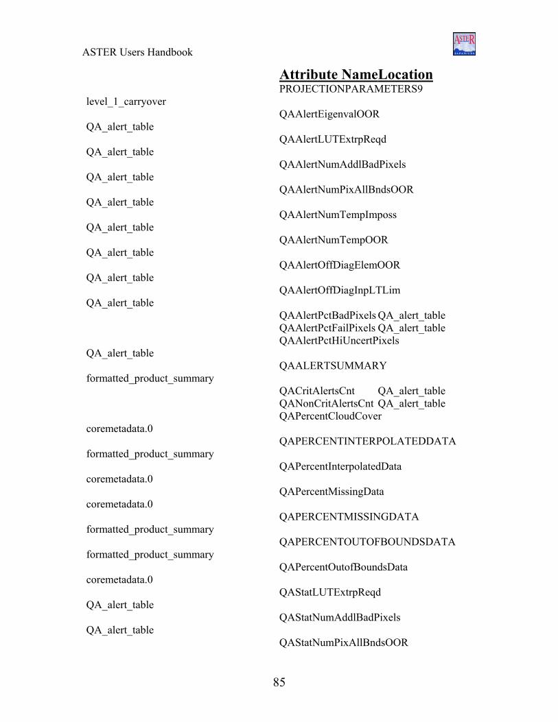
ASTER Users Handbook
Attribute Name Location PROJECTIONPARAMETERS9
level_1_carryover QAAlertEigenvalOOR
QA_alert_table QAAlertLUTExtrpReqd
QA_alert_table QAAlertNumAddlBadPixels
QA_alert_table QAAlertNumPixAllBndsOOR
QA_alert_table QAAlertNumTempImposs
QA_alert_table QAAlertNumTempOOR
QA_alert_table QAAlertOffDiagElemOOR
QA_alert_table QAAlertOffDiagInpLTLim
QA_alert_table QAAlertPctBadPixels QA_alert_table QAAlertPctFailPixels QA_alert_table QAAlertPctHiUncertPixels
QA_alert_table QAALERTSUMMARY
formatted_product_summary QACritAlertsCnt QA_alert_table QANonCritAlertsCnt QA_alert_table QAPercentCloudCover
coremetadata.0 QAPERCENTINTERPOLATEDDATA
formatted_product_summary QAPercentInterpolatedData
coremetadata.0 QAPercentMissingData
coremetadata.0 QAPERCENTMISSINGDATA
formatted_product_summary QAPERCENTOUTOFBOUNDSDATA
formatted_product_summary QAPercentOutofBoundsData
coremetadata.0 QAStatLUTExtrpReqd
QA_alert_table QAStatNumAddlBadPixels
QA_alert_table QAStatNumPixAllBndsOOR
85

ASTER Users Handbook
QA_alert_table QAStatNumTempOOR
QA_alert_table QAStatPctBadPixels QA_alert_table QAStatPctFailPixels QA_alert_table QAStatPctHiUncertPixels
QA_alert_table QASummaryOfAlerts QA_alert_table QuadrantCloudCoverage
productmetadata.0 QUADRANTCLOUDCOVERAGE
formatted_product_summary QUADRANTCLOUDCOVERAGE
level_1_carryover RadiometricDBVersion
productmetadata.0 RADIOMETRICDBVERSION
formatted_product_summary RECEIVINGCENTER
formatted_product_summary ReceivingCenter productmetadata.0 RecurrentCycleNumber
productmetadata.0
86
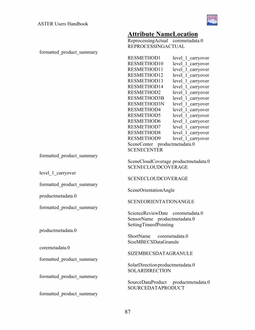
ASTER Users Handbook
Attribute Name Location ReprocessingActual coremetadata.0 REPROCESSINGACTUAL
formatted_product_summary RESMETHOD1 level_1_carryover RESMETHOD10 level_1_carryover RESMETHOD11 level_1_carryover RESMETHOD12 level_1_carryover RESMETHOD13 level_1_carryover RESMETHOD14 level_1_carryover RESMETHOD2 level_1_carryover RESMETHOD3B level_1_carryover RESMETHOD3N level_1_carryover RESMETHOD4 level_1_carryover RESMETHOD5 level_1_carryover RESMETHOD6 level_1_carryover RESMETHOD7 level_1_carryover RESMETHOD8 level_1_carryover RESMETHOD9 level_1_carryover SceneCenter productmetadata.0 SCENECENTER
formatted_product_summary SceneCloudCoverage productmetadata.0 SCENECLOUDCOVERAGE
level_1_carryover SCENECLOUDCOVERAGE
formatted_product_summary SceneOrientationAngle
productmetadata.0 SCENEORIENTATIONANGLE
formatted_product_summary ScienceReviewDate coremetadata.0 SensorName productmetadata.0 SettingTimeofPointing
productmetadata.0 ShortName coremetadata.0 SizeMBECSDataGranule
coremetadata.0 SIZEMBECSDATAGRANULE
formatted_product_summary SolarDirection productmetadata.0 SOLARDIRECTION
formatted_product_summary SourceDataProduct productmetadata.0 SOURCEDATAPRODUCT
formatted_product_summary
87

ASTER Users Handbook
SOURCEDATAPRODUCT level_1_carryover
SouthBoundingCoordinate coremetadata.0
SOUTHBOUNDINGCOORDINATE formatted_product_summary
SpatialResolution productmetadata.0
88

ASTER Users Handbook
Attribute Name Location SPATIALRESOLUTION
formatted_product_summary STANDARDDEVIATIONOFFSET10
level_1_carryover STANDARDDEVIATIONOFFSET11
level_1_carryover STANDARDDEVIATIONOFFSET12
level_1_carryover STANDARDDEVIATIONOFFSET13
level_1_carryover STANDARDDEVIATIONOFFSET14
level_1_carryover STANDARDDEVIATIONOFFSET4
level_1_carryover STANDARDDEVIATIONOFFSET5
level_1_carryover STANDARDDEVIATIONOFFSET6
level_1_carryover STANDARDDEVIATIONOFFSET7
level_1_carryover STANDARDDEVIATIONOFFSET8
level_1_carryover STANDARDDEVIATIONOFFSET9
level_1_carryover THRESHOLD10 level_1_carryover THRESHOLD11 level_1_carryover THRESHOLD12 level_1_carryover THRESHOLD13 level_1_carryover THRESHOLD14 level_1_carryover THRESHOLD4 level_1_carryover THRESHOLD5 level_1_carryover THRESHOLD6 level_1_carryover THRESHOLD7 level_1_carryover THRESHOLD8 level_1_carryover THRESHOLD9 level_1_carryover TIMEOFDAY formatted_product_summary TimeofDay coremetadata.0 UPPERLEFT formatted_product_summary UpperLeft productmetadata.0 UPPERRIGHT
formatted_product_summary UpperRight productmetadata.0 UTMZONECODE1 level_1_carryover UTMZONECODE10 level_1_carryover UTMZONECODE11 level_1_carryover
89

ASTER Users Handbook
UTMZONECODE12 level_1_carryover UTMZONECODE13 level_1_carryover UTMZONECODE14 level_1_carryover UTMZONECODE2 level_1_carryover UTMZONECODE3B level_1_carryover UTMZONECODE3N level_1_carryover
90
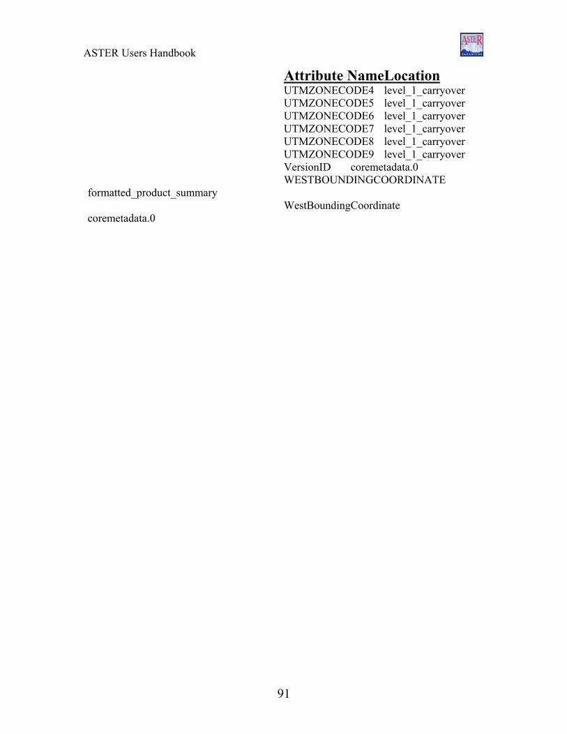
ASTER Users Handbook
Attribute Name Location UTMZONECODE4 level_1_carryover UTMZONECODE5 level_1_carryover UTMZONECODE6 level_1_carryover UTMZONECODE7 level_1_carryover UTMZONECODE8 level_1_carryover UTMZONECODE9 level_1_carryover VersionID coremetadata.0 WESTBOUNDINGCOORDINATE
formatted_product_summary WestBoundingCoordinate
coremetadata.0
91
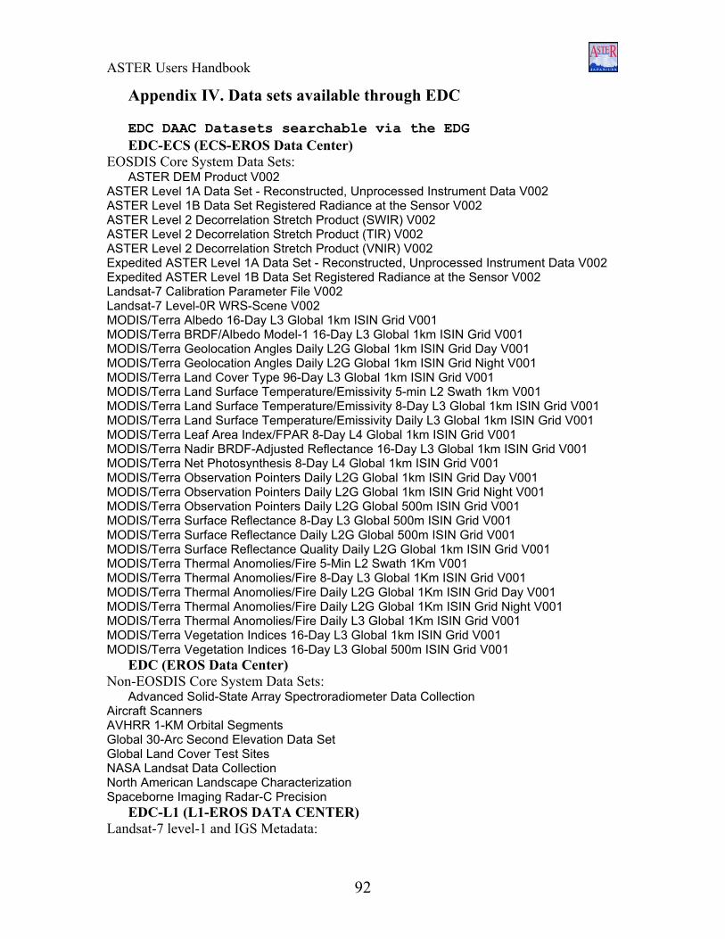
ASTER Users Handbook
Appendix IV. Data sets available through EDC EDC DAAC Datasets searchable via the EDG EDC-ECS (ECS-EROS Data Center)
EOSDIS Core System Data Sets: ASTER DEM Product V002
ASTER Level 1A Data Set - Reconstructed, Unprocessed Instrument Data V002 ASTER Level 1B Data Set Registered Radiance at the Sensor V002 ASTER Level 2 Decorrelation Stretch Product (SWIR) V002 ASTER Level 2 Decorrelation Stretch Product (TIR) V002 ASTER Level 2 Decorrelation Stretch Product (VNIR) V002 Expedited ASTER Level 1A Data Set - Reconstructed, Unprocessed Instrument Data V002 Expedited ASTER Level 1B Data Set Registered Radiance at the Sensor V002 Landsat-7 Calibration Parameter File V002 Landsat-7 Level-0R WRS-Scene V002 MODIS/Terra Albedo 16-Day L3 Global 1km ISIN Grid V001 MODIS/Terra BRDF/Albedo Model-1 16-Day L3 Global 1km ISIN Grid V001 MODIS/Terra Geolocation Angles Daily L2G Global 1km ISIN Grid Day V001 MODIS/Terra Geolocation Angles Daily L2G Global 1km ISIN Grid Night V001 MODIS/Terra Land Cover Type 96-Day L3 Global 1km ISIN Grid V001 MODIS/Terra Land Surface Temperature/Emissivity 5-min L2 Swath 1km V001 MODIS/Terra Land Surface Temperature/Emissivity 8-Day L3 Global 1km ISIN Grid V001 MODIS/Terra Land Surface Temperature/Emissivity Daily L3 Global 1km ISIN Grid V001 MODIS/Terra Leaf Area Index/FPAR 8-Day L4 Global 1km ISIN Grid V001 MODIS/Terra Nadir BRDF-Adjusted Reflectance 16-Day L3 Global 1km ISIN Grid V001 MODIS/Terra Net Photosynthesis 8-Day L4 Global 1km ISIN Grid V001 MODIS/Terra Observation Pointers Daily L2G Global 1km ISIN Grid Day V001 MODIS/Terra Observation Pointers Daily L2G Global 1km ISIN Grid Night V001 MODIS/Terra Observation Pointers Daily L2G Global 500m ISIN Grid V001 MODIS/Terra Surface Reflectance 8-Day L3 Global 500m ISIN Grid V001 MODIS/Terra Surface Reflectance Daily L2G Global 500m ISIN Grid V001 MODIS/Terra Surface Reflectance Quality Daily L2G Global 1km ISIN Grid V001 MODIS/Terra Thermal Anomolies/Fire 5-Min L2 Swath 1Km V001 MODIS/Terra Thermal Anomolies/Fire 8-Day L3 Global 1Km ISIN Grid V001 MODIS/Terra Thermal Anomolies/Fire Daily L2G Global 1Km ISIN Grid Day V001 MODIS/Terra Thermal Anomolies/Fire Daily L2G Global 1Km ISIN Grid Night V001 MODIS/Terra Thermal Anomolies/Fire Daily L3 Global 1Km ISIN Grid V001 MODIS/Terra Vegetation Indices 16-Day L3 Global 1km ISIN Grid V001 MODIS/Terra Vegetation Indices 16-Day L3 Global 500m ISIN Grid V001
EDC (EROS Data Center) Non-EOSDIS Core System Data Sets:
Advanced Solid-State Array Spectroradiometer Data Collection Aircraft Scanners AVHRR 1-KM Orbital Segments Global 30-Arc Second Elevation Data Set Global Land Cover Test Sites NASA Landsat Data Collection North American Landscape Characterization Spaceborne Imaging Radar-C Precision
EDC-L1 (L1-EROS DATA CENTER) Landsat-7 level-1 and IGS Metadata:
92

ASTER Users Handbook
93
Landsat-7 Level-0R IGS Scene Metadata V002 Landsat-7 Level-1 WRS-Scene V002