DPRIETI Discussion Paper Series 17-E-016

Assortative Matching of Exporters and Importers

SUGITA YoichiHitotsubashi University

TESHIMA KensukeInstituto Tecnológico Autónomo de México

Enrique SEIRAInstituto Tecnológico Autónomo de México

The Research Institute of Economy, Trade and Industryhttp://www.rieti.go.jp/en/

RIETI Discussion Paper Series 17-E-016

March 2017

Assortative Matching of Exporters and Importers1

SUGITA Yoichi

Hitotsubashi University

TESHIMA Kensuke

Instituto Tecnológico Autónomo de México

Enrique SEIRA

Instituto Tecnológico Autónomo de México

Abstract

We develop a novel approach to detect Beckerian positive assortative matching (PAM) of exporters

and importers by capability. Conventional approaches examining firm characteristics across matches

in cross-sectional data suffer from an endogeneity problem when firm characteristics reflect

unobserved partner characteristics. Instead, using the entry of new exporters induced by trade

liberalization as an exogenous shock to the capability rank of incumbent exporters, we investigate

resulting re-matching patterns among incumbent exporters and importers. Examining Mexico-U.S.

textile/apparel trade that experienced a surge in Chinese exporters after the Multi-Fibre Arrangement’s

end, we provide the first evidence for Beckerian PAM in exporter-importer relationships.

Keywords: Firm heterogeneity, Assortative matching, Two-sided heterogeneity, Trade liberalization

JEL classification: F1

RIETI Discussion Papers Series aims at widely disseminating research results in the form of professional

papers, thereby stimulating lively discussion. The views expressed in the papers are solely those of the

author(s), and neither represent those of the organization to which the author(s) belong(s) nor the Research

Institute of Economy, Trade and Industry.

1This study is conducted as a part of the Project “Analysis of Trade Costs” undertaken at the Research Institute of Economy, Trade and Industry (RIETI). We thank Andrew Bernard, Bernardo Blum, Kerem Cosar, Don Davis, Swati Dhingra, Lukasz Drozd, Meixin Guo, Daniel Halvarsson, Keith Head, Wen-Tai Hsu, Mathias Iwanowsky, Alberto Ortiz, Nina Pavcnik, James Rauch, Bob Rijkers, Esteban Rossi-Hansberg, Peter Schott, Yuta Suzuki, Heiwai Tang, Yong Tang, Catherine Thomas, Yuta Watabe, David Weinstein, Shintaro Yamaguchi, Makoto Yano, Yasutora Watanabe and seminar participants at numerous conferences and seminars. We thank Secretaría de Economía of México and the Banco de México for help with the data. Financial supports from the Private Enterprise Development in Low-Income Countries (PEDL), the Wallander Foundation, the Asociación Mexicana de Cultura, and JSPS KAKENHI (Grant Numbers 22243023 and 15H05392) are gratefully acknowledged. Francisco Carrera, Diego de la Fuente, Carlos Segura, and Stephanie Zonszein provided excellent research assistance.

1 Introduction

International trade mostly takes a form of firm-to-firm transaction. The empirical

trade literature have investigated firm’s trading behaviors in the last two decades and

established that firm’s capability such as productivity and product quality largely

determines the firm’s participation into exporting and importing.1 This paper con-

cerns a related open question whether firm’s capability also determines matching

of exporters and importers. More specifically, we examine whether matching of

exporters and importers in a product market follows positive assortative matching

(PAM) by capability a la Becker (1973). Beckerian PAM is a simple matching

mechanism based on transaction costs and complementarity. Although every firm

desires to match with high capability firms, a firm can only match with a limited

number of partners because of transaction costs. Because exporter’s and importer’s

capabilities exhibit complementarity, only high capability exporters can match with

high capability importers, while low capability exporters match with low capability

importers.

Beckerian PAM contrasts with the anonymous market in workhorse trade mod-

els that predicts no systematic matching.2 First, in the presence of complementarity,

the matching pattern of exporters and importers in Beckerian PAM has efficiency

implications, which is absent in the anonymous market. Second, Beckerian PAM

provides a guidance for trade promotion policies. Governments often encourage

local firms to trade with high capability foreign firms to improve local firms’ per-

formance through various channels.3 Beckerian PAM suggests the importance of1See, e.g., Bernard, Jensen, Redding, and Schott (2012) for their survey.2In perfectly competitive contexts such as in the Ricardian and Heckscher–Ohlin models, ex-

porters and importers are indifferent regarding who they trade with. The love of variety model alsoavoids positing any specific matching mechanism, instead predicting that all exporters will tradewith all importers.

3See e.g., De Loecker (2007) and Atkin, Khandelwal and Osman (2016) for learning technolo-gies; Takana (2016) for improving management practices; Machiavello (2010) and Machiavello and

1

capability development of local firms to realize their stable trade relationships with

high capability foreign firms.

In other matching contexts such as marriage, researchers often detect Beck-

erian PAM by examining exogenous characteristics of agents across matches in

regressions and/or structural models.4 However, two difficulties arises when one

applies this approach to the study of exporter–importer matching. The first diffi-

culty is specific to trade data. Data on the characteristics of exporters and importers

(e.g., manufacturing surveys covering multiple countries) are rarely available to re-

searchers together with data on matching patterns (e.g., customs transaction data).

The second difficulty is more broadly applied to the study of firm-to-firm matching

in general. Even if firm characteristics are available, in Beckerian PAM or other

non-anonymous markets, many of them (e.g., inputs, outputs) may reflect partner’s

unobserved capabilities as well as own capabilities, which makes it difficult to es-

timate individual firm’s capability.5 Most estimation methods of firm capability

such as TFP and product quality require no information about the buyers of each

seller, which in effect assumes the anonymous market where seller’s capability does

not depend on its buyers. With lack of reliable firm capability estimates, a naive

application of approaches in marriage research would suffer from an endogeneity

problem and not be informative about capability sorting.6

Morjaria (2015) for reputation building; Verhoogen (2008) for quality upgrading. The same ratio-nale is also discussed when promoting FDI (see e.g., Javorcik (2004) for vertical FDI spillovers).

4Choo and Siow (2006) is a pioneering study that structurally estimates Beckerian PAM in mar-riage. Graham (2011) and Chiappori and Salanie (2016) are recent surveys on econometrics ofmatching.

5For instance, the outputs and inputs of parts suppliers for Apple iPhone may increase in thesales of iPhone and thus may depend on Apple’s capability.

6Some might think of estimating exporter’s capability and importer’s capability by exporter fixedeffects and importer fixed effects of trade volume or other match-specific variables. This approachis analogous to Abowed, Kramarz and Margolis (1999, AKM) where the authors estimated un-observed worker skill and firm capability by worker fixed effects and firm fixed effects of wagepayment in matched employer-employee data. However, as Abowed, McKinney, and Schmutte(2015) emphasize, the AKM approach requires that workers move across firms independently of

2

To overcome these challenges, we develop a novel approach to detect the Beck-

erian PAM. Our approach requires only trade values for each product-level ex-

porter–importer matching, which are observable in many customs transaction datasets

and do not require augmenting with additional firm characteristics such as capa-

bility measures. The key innovation herein is that to cope with the endogeneity

problem, we use trade liberalization and the induced entry of new exporters as an

exogenous shock on the capability rank of incumbent exporters. Then, we interpret

how incumbent exporters and importers switch their partners in light of a simple

matching model to identify whether the matching is PAM, random matching, or

negative assortative matching (NAM). Another advantage of investigating trade lib-

eralization is that the degree of liberalization often differs across products within

industries. Thus, we can control for other factors commonly affecting matching

by comparing liberalized and non-liberalized products within industries. In sum,

we develop a clean empirical method for detecting exporter–importer PAM that is

implementable with a typical customs transaction dataset and a trade liberalization

episode.

We study matching between Mexican exporters and US importers in the tex-

tile/apparel product markets. Mexico–US textile/apparel trade is particularly suit-

able for our purpose. First, Mexican exporters and US importers mainly find their

foreign trading partners in each other. In 2004, the US was the largest market of

textile and apparel for Mexico, while Mexico was the second largest source for the

US.7 Second, at the disaggregated product (HS 6-digit) level, matching of Mexi-

can exporters and US importers in a given year is approximately one-to-one. This

skill and capability. Eeckhout and Kircher (2011) and De Melo (2016) show that when matchingfollows Beckerian PAM with endogenous worker mobility, firm fixed effects in the AKM approachbecome non-monotonic in firm capability and thus are difficult to interpret. Because of these recentdiscussions in labor economics, we do not pursue applying this two-way fixed effect approach toexporter–importer matching.

791.9% of Mexican exports are shipped to the US and 9.5% of US imports are from Mexico.

3

allows us to analyze firm’s choices of their main partners in a simple one-to-one

matching model. We show this new fact by using a novel index “main-to-main

share” in section 2. Finally, the Mexico–US textile/apparel trade experienced a

large and arguably exogenous trade liberalization shock due to the end of the Multi-

Fibre Arrangement (MFA). Following the schedule decided at the Uruguay round

of the GATT (1986–94), the US removed import quotas on approximately half of

the textile/apparel products against non-NAFTA countries in 2005, which resulted

in the massive entry of Chinese exporters at various capability levels into the US.

Our model combines the Becker (1973) model with a Melitz (2003)-type stan-

dard model of heterogeneous firm trade. The model consists of final producers (im-

porters) in the US and suppliers (exporters) in Mexico and China, all of whom are

heterogeneous in capability. A final producer and a supplier form a team under per-

fect information. Teams compete in the US final goods market under monopolistic

competition. Depending on whether team member capabilities exhibit complemen-

tarity, substitutability, or independence, stable matching becomes PAM, negative

assortative matching (NAM), or random matching, respectively. When new Chi-

nese suppliers enter at the MFA’s end, the capability rank of each Mexican exporter

among suppliers in the US falls, even if its absolute capability does not change. In

response to this exogenous change in capability ranks, the way incumbent Mexican

exporters and US importers change their partners differ across PAM, NAM, and

random matching. We mainly focus on PAM and random matching below (NAM

is discussed in the Appendix). Under PAM, Mexican exporters initially match with

US importers with the same capability rank in the US market. As the ranks of Mex-

ican exporters go down, Mexican exporters re-match with US importers with lower

capability, while US importers re-match with Mexican exporters with higher capa-

bility. We call this re-matching of Mexican exporters “partner downgrading” and

US importers “partner upgrading”. In contrast, under random matching, even with

4

negligible switching costs, US importers do not change their partners except when

the partners exit the US market.

We examine these predictions empirically in the following steps. We rank Mex-

ican exporters and US importers by their pre-liberalization product trade volumes

in 2004. The model predicts that under PAM and random matching, these rank-

ings should, on average, agree with the true rankings of capability. Using these

rankings, we compare partner switching patterns between liberalized products as

the treatment group and other textile/apparel products as the control group within

HS 2-digit industries. We confirm five predictions of PAM. First, US importers up-

grade their Mexican partners more often in the treatment group than in the control

group. Second, Mexican exporters downgrade US partners more often in the treat-

ment group than in the control group. Third, we do not find any systematic partner

change in other directions. Fourth, among firms who switched their main partners,

the capability ranks of the new partners are positively correlated with those of the

old partners. These together provide strong support for PAM and rejection of ran-

dom matching. Finally, the capability cutoff for Mexican exporters increases more

in the treatment group than in the control group, which is consistent with Melitz-

type models, including our model. We present numerous additional analyses that

support both the robustness of our results and the rejection of alternative explana-

tions.

This paper is related with the matching approach to modeling international

trade in non-anonymous markets. As pioneering studies, Rauch (1996), Casella

and Rauch (2002), and Rauch and Trindade (2003) developed Becker-type match-

ing models of exporters and importers by horizontally differentiated characteris-

tics. Antras, Garicano and Rossi-Hansberg (2006) and Sugita (2015) developed

models predicting PAM of exporters and importers by vertically differentiated ca-

pability. Our findings provide the first evidence for this matching approach using

5

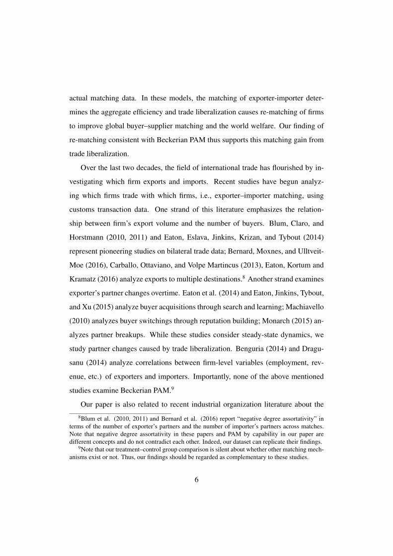
actual matching data. In these models, the matching of exporter-importer deter-

mines the aggregate efficiency and trade liberalization causes re-matching of firms

to improve global buyer–supplier matching and the world welfare. Our finding of

re-matching consistent with Beckerian PAM thus supports this matching gain from

trade liberalization.

Over the last two decades, the field of international trade has flourished by in-

vestigating which firm exports and imports. Recent studies have begun analyz-

ing which firms trade with which firms, i.e., exporter–importer matching, using

customs transaction data. One strand of this literature emphasizes the relation-

ship between firm’s export volume and the number of buyers. Blum, Claro, and

Horstmann (2010, 2011) and Eaton, Eslava, Jinkins, Krizan, and Tybout (2014)

represent pioneering studies on bilateral trade data; Bernard, Moxnes, and Ulltveit-

Moe (2016), Carballo, Ottaviano, and Volpe Martincus (2013), Eaton, Kortum and

Kramatz (2016) analyze exports to multiple destinations.8 Another strand examines

exporter’s partner changes overtime. Eaton et al. (2014) and Eaton, Jinkins, Tybout,

and Xu (2015) analyze buyer acquisitions through search and learning; Machiavello

(2010) analyzes buyer switchings through reputation building; Monarch (2015) an-

alyzes partner breakups. While these studies consider steady-state dynamics, we

study partner changes caused by trade liberalization. Benguria (2014) and Dragu-

sanu (2014) analyze correlations between firm-level variables (employment, rev-

enue, etc.) of exporters and importers. Importantly, none of the above mentioned

studies examine Beckerian PAM.9

Our paper is also related to recent industrial organization literature about the8Blum et al. (2010, 2011) and Bernard et al. (2016) report “negative degree assortativity” in

terms of the number of exporter’s partners and the number of importer’s partners across matches.Note that negative degree assortativity in these papers and PAM by capability in our paper aredifferent concepts and do not contradict each other. Indeed, our dataset can replicate their findings.

9Note that our treatment–control group comparison is silent about whether other matching mech-anisms exist or not. Thus, our findings should be regarded as complementary to these studies.

6

role of firm characteristics in determining firm-to-firm networks, which encompass

matching and mergers. Using a revealed preference approach developed by Fox

(2016), recent papers structurally estimate matching/merger surplus functions (e.g.

Akkus, Cookson and Hortacsu 2015; Nakajima, 2012). The Fox approach and our

approach both assume frictionless matching models with transferable utility as in

Becker (1973).10 The main difference is that while the Fox approach analyzes the

relative importance of multiple firm characteristics, our approach using a natural ex-

periment precisely examines one factor of interest. Thus, we see the two approaches

are complementary and could be fruitfully combined in future research.

The rest of the paper is organized as follows. Section 2 discusses our data and

the two features of the Mexico–US textile/apparel trade that motivate our analysis:

the end of the Multi-Fibre Arrangement and approximately one-to-one matching

of exporters and importers at the product level. Section 3 presents our model and

derives predictions. Section 4 describes our empirical strategies. Section 5 presents

the main empirical results and robustness checks. Section 6 is the conclusion. The

online Appendix provides calculations, proofs, data construction, summary statis-

tics, and additional analyses rejecting alternative explanations for our results.

2 Mexico–US Textile Apparel Trade

2.1 End of the Multi-Fibre Arrangement

The Mexico–US textile/apparel trade experienced large-scale trade liberalization in

2005, the end of the Multi-Fibre Arrangement (MFA). The MFA and its successor,

the Agreement on Textile and Clothing, are agreements on quota restrictions regard-

ing textile/apparel imports among GATT/WTO member countries. At the GATT10Studies on matching using non-transferable utility frameworks include Sorensen (2007) on ven-

ture capitals and Uetake and Watanabe (2012) on Bank mergers.

7

Uruguay round, the US (together with Canada, the EU, and Norway) promised to

abolish their quotas in four steps (1995, 1998, 2002, and 2005). At each removal,

liberalized products constituted 16, 17, 18, and 49% of imports in 1990, respec-

tively. The end of the MFA in 2005 is the largest liberalization.

We highlight three facts from previous studies that motivate our analysis.

Fact 1: Surge in Chinese Exports to the US According to Brambilla, Khan-

delwal, and Schott (2010), US imports from China disproportionally increased by

271% in 2005, whereas imports from almost all other countries decreased. Using

data by Brambilla et al. (2010) on US import quotas, we classify each HS 6-digit

textile/apparel product into one of two groups [see Appendix for details]. The first

treatment group consists of products for which Chinese exports to the US are sub-

ject to a binding quota in 2004, while the second control group consists of other

textile/apparel products. The left panel in Figure 1 displays Chinese exports to the

US from 2000 to 2010 for the treatment group with a dashed line and the control

group with a solid line. After the 2005 quota removal, Chinese exports of the treat-

ment group increased much faster than those of the control group.11

Fact 2: Exports by New Chinese Entrants with Various Capability Levels Us-

ing Chinese customs transaction data, Khandelwal, Schott, and Wei (2013) decom-

pose the increases in Chinese exports to US, Canada, and the EU after the quota

removal into intensive and extensive margins. They find that increases in Chinese

exports belonging to the treatment group were mostly driven by the entry of Chinese

exporters who had not previously exported these products. Furthermore, these new11Seeing this substantial surge in import growth, the US and China had agreed to impose new

quotas until 2008, but imports from China never dropped back to their pre-2005 levels. This isbecause (1) the new quota system covered fewer product categories than the old system (Dayaranta-Banda and Whalley, 2007), and (2) the new quotas levels were substantially greater than MFA levels(see Table 2 in Brambilla et al., 2010).

8

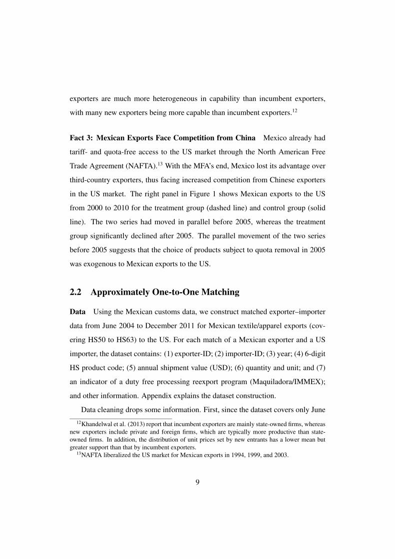
exporters are much more heterogeneous in capability than incumbent exporters,

with many new exporters being more capable than incumbent exporters.12

Fact 3: Mexican Exports Face Competition from China Mexico already had

tariff- and quota-free access to the US market through the North American Free

Trade Agreement (NAFTA).13 With the MFA’s end, Mexico lost its advantage over

third-country exporters, thus facing increased competition from Chinese exporters

in the US market. The right panel in Figure 1 shows Mexican exports to the US

from 2000 to 2010 for the treatment group (dashed line) and control group (solid

line). The two series had moved in parallel before 2005, whereas the treatment

group significantly declined after 2005. The parallel movement of the two series

before 2005 suggests that the choice of products subject to quota removal in 2005

was exogenous to Mexican exports to the US.

2.2 Approximately One-to-One Matching

Data Using the Mexican customs data, we construct matched exporter–importer

data from June 2004 to December 2011 for Mexican textile/apparel exports (cov-

ering HS50 to HS63) to the US. For each match of a Mexican exporter and a US

importer, the dataset contains: (1) exporter-ID; (2) importer-ID; (3) year; (4) 6-digit

HS product code; (5) annual shipment value (USD); (6) quantity and unit; and (7)

an indicator of a duty free processing reexport program (Maquiladora/IMMEX);

and other information. Appendix explains the dataset construction.

Data cleaning drops some information. First, since the dataset covers only June12Khandelwal et al. (2013) report that incumbent exporters are mainly state-owned firms, whereas

new exporters include private and foreign firms, which are typically more productive than state-owned firms. In addition, the distribution of unit prices set by new entrants has a lower mean butgreater support than that by incumbent exporters.

13NAFTA liberalized the US market for Mexican exports in 1994, 1999, and 2003.

9

to December for 2004, we drop observations from January to May for other years

to make each year’s information comparable. Similar results are obtained with

January–May data. Second, we drop exporters who do not report importer informa-

tion for most transactions. These exporters use the Maquiladora/IMMEX program

where exporters do not have to report an importer for each shipment.14 Luckily, a

substantial number of Maquiladora/IMMEX exporters do report importer informa-

tion. To address potential selection issues, we compare these Maquiladora/IMMEX

exporters and other normal exporters in almost all empirical analyses below.

Approximately One-to-One Matching at Product Level Table 1 reports mean

and median statistics about product-level matching. While Rows (1) and (2) show

that an average product has 11–15 exporters and 15–20 importers, Rows (3) and

(4) show that the majority of firms trade with only one partner.15 Rows (5) and (6)

show that even firms who trade with multiple partners concentrate more than 70%

of trade volume with their single main partner. In sum, most firms conduct most of

their trade with only one partner in a given year.

Furthermore, product-level matching between Mexican exporters and US im-

porters is approximately one-to-one. We develop a new measure “main-to-main

share,” which expresses the extent to which overall transactions in one product

market are quantitatively close to one-to-one matching. We define a “main-to-main

match” as a product-level match in which the exporter is the main partner of the

importer for the product, while simultaneously, the importer is the main partner of14The Maquiladoras program started in 1986 and was replaced by the IMMEX (Industria Man-

ufacturera, Maquiladora y de Servicios de Exportation) program in 2006. In the Maquilado-ras/IMMEX programs, firms in Mexico can import materials and equipment duty free used forproducts exported. Exporters must register importer’s information in advance but do not need toreport it for each shipment.

15Numbers in Rows (1) to (4) in Table 1 appear smaller than those in Blum et al. (2010, 2011),Bernard et al. (2013), and Carballo et al. (2013). When a match is defined at the country level asthey do, these numbers in our data become similar to those in these studies.

10

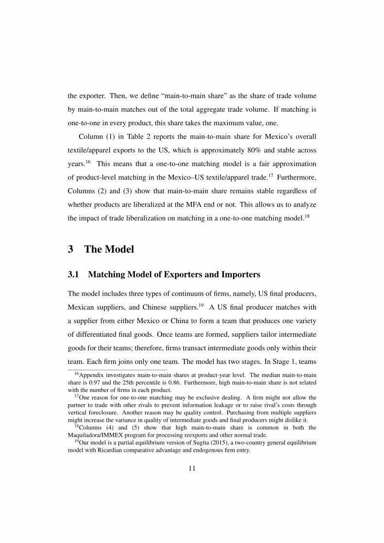
the exporter. Then, we define “main-to-main share” as the share of trade volume

by main-to-main matches out of the total aggregate trade volume. If matching is

one-to-one in every product, this share takes the maximum value, one.

Column (1) in Table 2 reports the main-to-main share for Mexico’s overall

textile/apparel exports to the US, which is approximately 80% and stable across

years.16 This means that a one-to-one matching model is a fair approximation

of product-level matching in the Mexico–US textile/apparel trade.17 Furthermore,

Columns (2) and (3) show that main-to-main share remains stable regardless of

whether products are liberalized at the MFA end or not. This allows us to analyze

the impact of trade liberalization on matching in a one-to-one matching model.18

3 The Model

3.1 Matching Model of Exporters and Importers

The model includes three types of continuum of firms, namely, US final producers,

Mexican suppliers, and Chinese suppliers.19 A US final producer matches with

a supplier from either Mexico or China to form a team that produces one variety

of differentiated final goods. Once teams are formed, suppliers tailor intermediate

goods for their teams; therefore, firms transact intermediate goods only within their

team. Each firm joins only one team. The model has two stages. In Stage 1, teams16Appendix investigates main-to-main shares at product-year level. The median main-to-main

share is 0.97 and the 25th percentile is 0.86. Furthermore, high main-to-main share is not relatedwith the number of firms in each product.

17One reason for one-to-one matching may be exclusive dealing. A firm might not allow thepartner to trade with other rivals to prevent information leakage or to raise rival’s costs throughvertical foreclosure. Another reason may be quality control. Purchasing from multiple suppliersmight increase the variance in quality of intermediate goods and final producers might dislike it.

18Columns (4) and (5) show that high main-to-main share is common in both theMaquiladora/IMMEX program for processing reexports and other normal trade.

19Our model is a partial equilibrium version of Sugita (2015), a two-country general equilibriummodel with Ricardian comparative advantage and endogenous firm entry.

11

are formed under perfect information. In Stage 2, teams compete in the US final-

good market in a monopolistically competitive fashion.

Firms’ capabilities are heterogeneous. Capability reflects productivity and/or

quality. Let x and y be the capability of final producers and suppliers, respectively.

There exist a fixed mass MU

of final producers in the US, MM

of suppliers in Mex-

ico, and MC

of suppliers in China. The cumulative distribution function (c.d.f.) for

the capability of US final producers is F (x) with continuous support [xmin

, xmax

].

The capability of Mexican and Chinese suppliers follows an identical distribution,

and the c.d.f. is G(y) with continuous support [ymin

, ymax

].20 For simplicity, a Chi-

nese supplier is a perfect substitute for a Mexican supplier of the same capability.

Teams’ capabilities are heterogeneous. Team capability ✓(x, y) increases in

members’ capability, ✓1 ⌘ @✓(x, y)/@x > 0 and ✓2 ⌘ @✓(x, y)/@y > 0. Matching

endogenously determines the distribution of ✓.

The US representative consumer maximizes the following utility function:

U =

�

⇢lnZ

!2⌦✓(!)↵q(!)⇢d!

�+ q0 s.t.

Z

!2⌦p(!)q(!)d! + q0 = I.

where ⌦ is a set of available differentiated final goods, ! is a variety of differ-

entiated final goods, p (!) is the price of !, q(!) is the consumption of !, ✓(!)

is the capability of a team producing !, q0 is the consumption of a numeraire

good, I is an exogenously given income. ↵ � 0 and � > 0 are given parame-

ters. Consumer demand for a variety with price p and capability ✓ is derived as

q(p, ✓) = �✓↵�P ��1p��, where � ⌘ 1/ (1� ⇢) > 1 is the elasticity of substitution

and P ⌘⇥R

!2⌦ p(!)1��✓ (!)↵� d!⇤1/(1��) is the price index.

Production technology is of Leontief type. When a team with capability ✓ pro-20An identical capability distribution of Chinese and Mexican suppliers is assumed for graphical

exposition and is not essential for the main predictions.

12

duces q units of final goods, the team supplier produces q units of intermediate

goods with costs cy

✓�q + fy

; then, the final producer assembles these intermediate

goods into final goods with costs cx

✓�q + fx

, where ci

and fi

are positive constants

(i = x, y). Team’s total costs are c(✓, q) = c✓�q + f, where c ⌘ cx

+ cy

and

f ⌘ fx

+ fy

. Externalities within teams make firms’ marginal costs dependent on

both their partner’s capability and their own capability.21 For simplicity, we assume

firm’s marginal costs depend on the team’s capability.

Team capability ✓ may represent productivity and/or quality, depending on ↵

and �. For instance, when ↵ = 0 and � < 0, teams face symmetric demand and a

high value for ✓ implies lower marginal costs. In this case, ✓ represents productivity

(e.g., Melitz, 2003). When ↵ > 0 and � > 0, a high value of ✓ implies a large

demand at a given price and high marginal costs. In this case, ✓ may be called

quality (e.g., Baldwin and Harrigan, 2011; Johnson, 2012; Verhoogen, 2008).

Backward induction obtains an equilibrium (see Appendix for calculations).

Stage 2 Team’s optimal price is p(✓) = c✓�/⇢. Hence, team revenue R(✓), total

costs C(✓), and joint profits ⇧ (✓) are

R(✓) = �A✓�, C(✓) = (� � 1)A✓� + f, and ⇧ (✓) = A✓� � f. (1)

where A ⌘ �

�

�⇢P

c

���1 summarizes factors that (infinitesimal) individual teams take

as given. We assume � ⌘ ↵�� � (� � 1) > 0 so that team profits are increasing in

team capability. Furthermore, we normalize � = 1 by choosing the unit of ✓ as com-

parative statics on ↵, �, and � is not our main interest. Let M and H(✓) be the mass21An example of a within-team externality is costs of quality control. Producing high quality final

goods might require extra costs of quality control at each production stage because even one de-fective component can destroy the whole product (Kremer, 1993). Another example is productivityspillovers. Through teaching and learning (e.g. joint R&D) within a team, each member’s marginalcost may depend on the entire team’s capability.

13

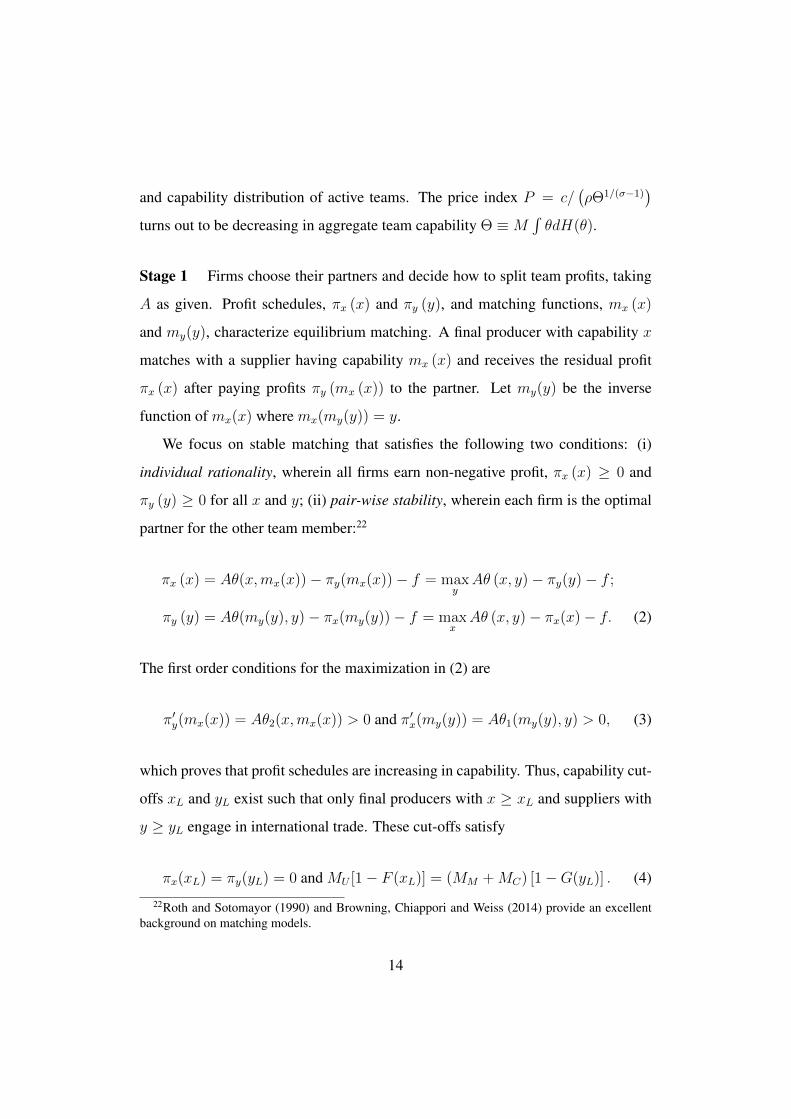
and capability distribution of active teams. The price index P = c/�⇢⇥1/(��1)

�

turns out to be decreasing in aggregate team capability ⇥ ⌘ MR✓dH(✓).

Stage 1 Firms choose their partners and decide how to split team profits, taking

A as given. Profit schedules, ⇡x

(x) and ⇡y

(y), and matching functions, mx

(x)

and my

(y), characterize equilibrium matching. A final producer with capability x

matches with a supplier having capability mx

(x) and receives the residual profit

⇡x

(x) after paying profits ⇡y

(mx

(x)) to the partner. Let my

(y) be the inverse

function of mx

(x) where mx

(my

(y)) = y.

We focus on stable matching that satisfies the following two conditions: (i)

individual rationality, wherein all firms earn non-negative profit, ⇡x

(x) � 0 and

⇡y

(y) � 0 for all x and y; (ii) pair-wise stability, wherein each firm is the optimal

partner for the other team member:22

⇡x

(x) = A✓(x,mx

(x))� ⇡y

(mx

(x))� f = max

y

A✓ (x, y)� ⇡y

(y)� f ;

⇡y

(y) = A✓(my

(y), y)� ⇡x

(my

(y))� f = max

x

A✓ (x, y)� ⇡x

(x)� f. (2)

The first order conditions for the maximization in (2) are

⇡0y

(mx

(x)) = A✓2(x,mx

(x)) > 0 and ⇡0x

(my

(y)) = A✓1(my

(y), y) > 0, (3)

which proves that profit schedules are increasing in capability. Thus, capability cut-

offs xL

and yL

exist such that only final producers with x � xL

and suppliers with

y � yL

engage in international trade. These cut-offs satisfy

⇡x

(xL

) = ⇡y

(yL

) = 0 and MU

[1� F (xL

)] = (MM

+MC

) [1�G(yL

)] . (4)22Roth and Sotomayor (1990) and Browning, Chiappori and Weiss (2014) provide an excellent

background on matching models.

14

The second condition in (4) indicates that the number of suppliers in the matching

market is equal to the number of final producers.

Differentiating the first order condition (3) by x, we obtain

m0x

(x) =A✓12

⇡00y

� A✓22, where ✓12 ⌘

@2✓

@x@yand ✓22 ⌘

@2✓

@y2.

Since the denominator is positive from the second order condition, the sign of cross

derivatives ✓12 is the same as the sign of m0x

(x), i.e. the sign of sorting in stable

matching (e.g., Becker, 1973). For simplicity, we consider three cases where the

sign of ✓12 is constant for all x and y: (1) Case C (Complement) ✓12 > 0; (2) Case

I (Independent) ✓12 = 0; (3) Case S (Substitute) ✓12 < 0.23 In Case C, we have

positive assortative matching (PAM) (m0x

(x) > 0): high capability firms match with

high capability firms whereas low capability firms match low capability firms. In

Case S, we have negative assortative matching (NAM) (m0x

(x) < 0): high capability

firms match low capability firms. In Case I, we cannot determine a matching pattern

[i.e., mx

(x) cannot be defined as a function] because each firm is indifferent about

partner capability. Therefore, we assume matching is random in Case I. Case I is

a useful benchmark because it nests traditional models where firm heterogeneity

exists only for one side of the market, i.e., either among exporters (✓1 = ✓12 = 0)

or among importers (✓2 = ✓12 = 0). We focus on Case C and Case I in the main

text of the paper and discuss Case S in the Appendix.23In Case C and Case S, ✓ is also called strict supermodular and strict submodular, respectively.

An example for Case C is the complementarity of quality of tasks in a production process (e.g.,Kremer, 1993). For instance, a high-quality car part is more useful when combined with other high-quality car parts. An example for Case S is technological spillovers through learning and teaching.Gains from learning from high capable partners might be greater for low capability firms. See e.g.,Grossman and Maggi (2000) for further examples on Case C and Case S.

15

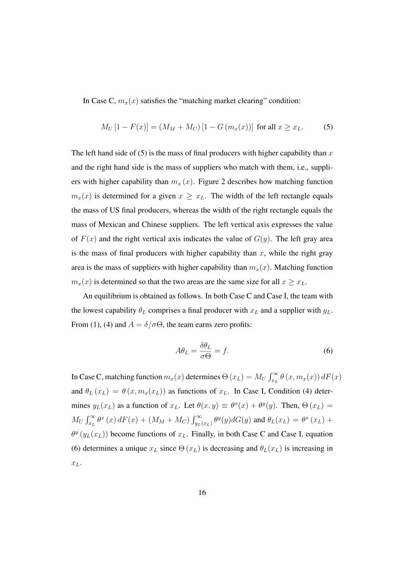
In Case C, mx

(x) satisfies the “matching market clearing” condition:

MU

[1� F (x)] = (MM

+MC

) [1�G (mx

(x))] for all x � xL

. (5)

The left hand side of (5) is the mass of final producers with higher capability than x

and the right hand side is the mass of suppliers who match with them, i.e., suppli-

ers with higher capability than mx

(x). Figure 2 describes how matching function

mx

(x) is determined for a given x � xL

. The width of the left rectangle equals

the mass of US final producers, whereas the width of the right rectangle equals the

mass of Mexican and Chinese suppliers. The left vertical axis expresses the value

of F (x) and the right vertical axis indicates the value of G(y). The left gray area

is the mass of final producers with higher capability than x, while the right gray

area is the mass of suppliers with higher capability than mx

(x). Matching function

mx

(x) is determined so that the two areas are the same size for all x � xL

.

An equilibrium is obtained as follows. In both Case C and Case I, the team with

the lowest capability ✓L

comprises a final producer with xL

and a supplier with yL

.

From (1), (4) and A = �/�⇥, the team earns zero profits:

A✓L

=

�✓L

�⇥= f. (6)

In Case C, matching function mx

(x) determines ⇥ (xL

) = MU

R1x

L

✓ (x,mx

(x)) dF (x)

and ✓L

(xL

) = ✓ (x,mx

(xL

)) as functions of xL

. In Case I, Condition (4) deter-

mines yL

(xL

) as a function of xL

. Let ✓(x, y) ⌘ ✓x(x) + ✓y(y). Then, ⇥ (xL

) =

MU

R1x

L

✓x (x) dF (x) + (MM

+MC

)

R1y

L

(xL

) ✓y

(y)dG(y) and ✓L

(xL

) = ✓x (xL

) +

✓y (yL

(xL

)) become functions of xL

. Finally, in both Case C and Case I, equation

(6) determines a unique xL

since ⇥ (xL

) is decreasing and ✓L

(xL

) is increasing in

xL

.

16

3.2 Consequences of Chinese Firm Entry at the End of the MFA

We analyze the impact of Chinese firm entries at the end of the MFA on matching

between US importers and Mexican exporters. As discussed in Section 2.3, new

entrants are heterogeneous in capability. Thus, we model this event as an exogenous

increase in the mass of Chinese suppliers (dMC

> 0) in the US market. We assume

positive but negligible costs for switching partners so that a firm changes its partner

only if it strictly prefers the new match over the current match.

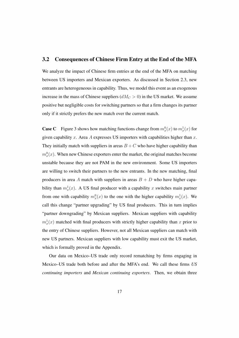
Case C Figure 3 shows how matching functions change from m0x

(x) to m1x

(x) for

given capability x. Area A expresses US importers with capabilities higher than x.

They initially match with suppliers in areas B+C who have higher capability than

m0x

(x). When new Chinese exporters enter the market, the original matches become

unstable because they are not PAM in the new environment. Some US importers

are willing to switch their partners to the new entrants. In the new matching, final

producers in area A match with suppliers in areas B + D who have higher capa-

bility than m1x

(x). A US final producer with a capability x switches main partner

from one with capability m0x

(x) to the one with the higher capability m1x

(x). We

call this change “partner upgrading” by US final producers. This in turn implies

“partner downgrading” by Mexican suppliers. Mexican suppliers with capability

m1x

(x) matched with final producers with strictly higher capability than x prior to

the entry of Chinese suppliers. However, not all Mexican suppliers can match with

new US partners. Mexican suppliers with low capability must exit the US market,

which is formally proved in the Appendix.

Our data on Mexico–US trade only record rematching by firms engaging in

Mexico–US trade both before and after the MFA’s end. We call these firms US

continuing importers and Mexican continuing exporters. Then, we obtain three

17

predictions for Case C as follows.

C1: US continuing importers switch their Mexican partners to those with higher

capability (partner upgrading), while Mexican continuing exporters switch

their US partners to those with lower capability (partner downgrading).

C2: PAM holds both before and after the MFA’s end.

C3: The capability cutoff for Mexican exporters rises.

Case I Entry of Chinese suppliers also raises the capability cutoff yL

for suppliers

so that low capability suppliers exit, which is proved in the Appendix. US importers

who matched with these exiting suppliers switch to new Chinese suppliers. Other

firms continue to match with their old partners, though they change price and quan-

tity of goods traded. This is because firms are indifferent about their partners as long

as they have higher capability than the cutoffs. Thus, we obtain three predictions.

I1: US continuing importers do not change their Mexican partners, while Mexican

continuing exporters do not change their US partners.

I2: Matching is random before and after the MFA’s end.

I3: The capability cutoff for Mexican exporters rises.

Rematching Gain from Trade The end of the MFA causes two adjustments.

First, new Chinese suppliers with high capability replace Mexican suppliers with

low capability (replacement effect), which exists in both Cases C and I. Second,

continuing firms re-match (rematching effect), which exists in Case C but not in

Case I. We show both adjustments lower the price index and benefits the consumer.

18

To see each adjustment, we consider a hypothetical “no-rematching” equilib-

rium where no rematching occurs and where firms switch partners only if their cur-

rent partner exits the market. Denote variables in this no-rematching equilibrium

by “NR,” variables before the MFA’s end by “B,” and variables after the MFA’s end

by “A.” Then, the change in the price index PB � PA is decomposed into the re-

placement effect PB � PNR and the rematching effect PNR � PA. The following

lemma establishes these two effects (the proof is in the Appendix).

Lemma 1. In Case C, PA < PNR < PB, while in Case I, PA

= PNR < PB.

In Case C, the rematching effect is positive, i.e., the rematching creates an addi-

tional consumer gain. From P = c/�⇢⇥1/(��1)

�, this gain comes from increases in

the aggregate capability, ⇥A > ⇥

NR > ⇥

B, which arises from a classic theorem in

the matching theory that a stable matching maximizes aggregate payoffs, A⇥�Mf ,

(Koopmans and Beckmann, 1957; Shapley and Shubik, 1972; Gretsky, Ostroy and

Zame, 1992). In Case I, the rematching effect is zero because matching is irrele-

vant. If data observe rematching consistent with Case C, the model interprets it as a

process of improving global buyer–supplier matching and rasing consumer welfare.

4 Empirical Strategies

4.1 Proxy for Capability Rankings

Testing predictions C1-C3 and I1-I3 requires data on firm capability. We use firm

trade volumes as a proxy for firm capability, using properties of the model.

For Case C, let I(x) be the import volume by an US importer with capability

x and let X(y) be the export volume by a Mexican exporter with capability y. For

Case I, let ¯I(x) be the expected import volume by a US importer with capability x

19

and let ¯X(y) be the expected export volume by a Mexican exporters with capability

y. Then, using the fact that within team trade T (x, y) is increasing in x and y, we

obtain the following lemma for the monotonic relationship between firm capability

and trade volume (the proof is in Appendix).

Lemma 2. In Case C, I(x) and X(y) are strictly increasing functions. In Case I,

¯I(x) and ¯X(y) are strictly increasing functions.

For each product, we create a ranking of US continuing importers by the amount

of their imports from their main partner in 2004 before the MFA’s end. Similarly, for

each product, we rank Mexican continuing exporters by the amount of their exports

to their main partner in 2004. From Lemma 2, these rankings should agree with the

rankings of true capability in Case C and on average so in Case I. We assume that

the capability ranking is stable in a short run and thus use the rank measured from

2004 data for the same firm throughout our sample period.24

Using these rankings, we first create three variables: (1) firm i’s own rank in

product g in country c, OwnRankc

ig

; (2) rank of the firm’s main partner of product g

in 2004 before the MFA’s end, OldPartnerRankc

ig

; and (3) rank of the firm’s main

partner of product g in 2007 after the MFA’s end, NewPartnerRankc

ig

.25 Note

that OldPartnerRankc

ig

differs from NewPartnerRankc

ig

if and only if the firm

switches the main partner during 2004–07. These ranks are standardized using the

number of firms so as to fall in [0,1]. Smaller ranks indicate higher capability. Fi-

nally, we create variables of partner changes as follows. Partner upgrading dummy

Upcigs

equals one if NewPartnerRankigs

< OldPartnerRankigs

. Partner down-

grading dummy Downc

igs

equals one if NewPartnerRankigs

> OldPartnerRankigs

.

24Trade volume ranks in 2004 and 2007 are highly correlated, which confirms our assumption.All correlation coefficients are above 0.85 and similar between the treatment and control groups.

25We choose the period of 2004-07 because the 2008 Lehman crisis, which greatly reduced Mex-ican exports to the US, potentially confounds the impact of the MFA end.

20

4.2 Specifications

Partner Changes (C1 and I1) We estimate the following regressions to test pre-

dictions C1 and I1 on partner changes:

Upcigs

= �c

U

Bindinggs

+ �s

+ "cUigs

Downc

igs

= �c

D

Bindinggs

+ �s

+ "cDigs

, (7)

where c, i, g, and s represent a country (US and Mexico), firm, HS 6-digit product,

and sector (HS 2-digit level), respectively. Dummy variable Bindinggs

equals one

if Chinese exports of product g to the US faced a binding quota in 2004, which

is constructed from Brambilla et al. (2010). �s

represents HS 2-digit level fixed

effects.26 uc

igs

and "cijs

are error terms. Appendix explains the construction of the

binding dummy and other variables.

The coefficients of interest in (7) are �c

U

and �c

D

. With HS 2-digit product fixed

effects, these coefficients are identified by comparing treatment and control groups

within the same HS 2-digit sectors. The treatment is the removal of binding quotas

on Chinese exports to the US. The coefficients �c

U

and �c

D

estimate its impact on the

probability that firms will switch from their initial main partner to one with higher

and lower capabilities, respectively.

Prediction I1 for random matching states that in response to the MFA’s end, con-

tinuing US importers and Mexican exporters would not change their partners at all.

In reality, other shocks that could induce partner changes may exist. Considering

this point, we reformulate Prediction I1: no difference should exist in the probabil-

ity of partner changes in any direction between treatment and control groups. This

prediction corresponds to �US

U

= �US

D

= �Mex

U

= �Mex

D

= 0 in (7).26We drop HS 2-digit sectors (HS 50, 51, 53, 56, 57, and 59) in which no variation of the binding

dummy at HS 2-digit level occurs.

21

Prediction C1 for PAM states that in response to the MFA’s end, all continu-

ing US importers upgrade whereas all continuing Mexican exporters downgrade

their main partners. Though the frictionless matching model predicts all firms will

change their partners, in reality, other factors such as transaction costs are likely

to prevent some firms from making such a change, at least in the short run. Ac-

cordingly, we reformulate Prediction C1 as follows: US importers’ partner up-

grading and Mexican exporters’ partner downgrading will occur more frequently

in the treatment group than in the control group, which corresponds to �US

U

> 0,

�US

D

= �Mex

U

= 0, and �Mex

D

> 0 in (7).

Our regression (7) does not suffer from the endogeneity problem that existed in

the conventional correlation approach of regressing exporter’s characteristics on im-

porter’s. We use firm characteristics (trade volume) only to construct the outcome

variables in the left hand side, not any variable in the right hand side. Any dis-

crepancy between the true capability ranking and the trade volume ranking should

appear in error terms "cUigs

and "cDigs

, which might reflect own capability, partner’s

capability and other unobservable firm and product characteritics. However, as long

as the binding dummy is uncorrelated with these unobservable characteristics, �c

U

and �c

D

are consistently estimated.

Old and New Partner Ranks (C2 and I2) To test predictions C2 and I2, we

estimate the following regression for firms who switched partners during 2004-07:

NewPartnerRankc

ig

= ↵c

+ �cOldPartnerRankc

ig

+ "cig

(8)

for firm iwith NewPartnerRankc

ig

6= OldPartnerRankc

ig

.

Prediction C2 states that PAM holds both before and after the MFA’s end. New

partner ranks should be positively correlated with old partner ranks, i.e., �c > 0.

22

Predictions I2 states that matching is random before and after the MFA’s end. Thus,

there should be no correlation among them, i.e., �c

= 0.

Two additional points need to be mentioned. First, if we run (8) only for firms

that do not change partners, then �c equals to one by construction. To avoid this

mechanical correlation, we estimate (8) only for firms who change partners. Sec-

ond, the regression (8) combines both the treatment and control groups since PAM

should hold for both groups in Case C.27

Capability Cutoff Changes (C3 and I3) Finally, we test predictions C3 and I3

that the capability cutoff for Mexican exporters rises in the treatment group. While

the MFA’s end is the only shock occuring in the model, other shocks might occur

that induce firm exit from the market. Indeed, it is observed in many datasets that

entry and exit of exporting simlutanously occur even without trade liberalization

(e.g., Eaton et. al., 2014). To address this possibility, we consider a simple threshold

model of exit behavior. In each period r, Mexican supplier i receives a random i.i.d.

shock "ir

to its profits, which captures idiosyncratic factors inducing firm exit in

absence of trade liberalization. The firm chooses to exit if "ir

is below a threshold

"̄ir

(y), that is, firm i’s exit probability is Pr [" < "̄ir

(y)]. Case C and Case I have

two predictions: (i) threshold "̄ir

(y) is a decreasing function in the firm’s capability

y; and (ii) the MFA’s end increases threshold "̄ir

(y) for a given capability y.

To control for intrinsic differences between treatment and control groups, we

conduct a difference-in-difference comparison of firm exit rates between groups for

two periods, namely pre-liberalization (2001–04) and post-liberalization (2004–07).

Since Mexican customs data before 2004 have no (digitized) record on importers,

we use Mexican exporter’s total product export volumes as a proxy for capability,27For instance, if an industry-wide shock induces Mexican exporter’s partner to downgrade in

both treatment and control groups, the model with PAM should predict �c > 0 for both groups.

23

which is highly correlated with exports with the main partners in the 2004–07 data.

Then, we estimate the following regression for Mexican firm i who exports product

g to the US in the initial year of period r 2 {2001� 04, 2004� 07}:

Exitigsr

= �1Bindingg

+ �2Bindingg

⇤ Afterr

+ �3Afterr + �4 lnExportsigr

+ �5Afterr ⇤ lnExportsigr

+ �s

+ uigsr

. (9)

Dummy variable Exitigsr

equals one if the firm stops exporting during period r.

Dummy variable Afterr

equals one if period r is 2004–07. lnExportsigr

is the

log of the firm’s total export volume of product g in the initial year of period r,

which proxies firm capability.28 �s

represents HS 2-digit level fixed effects and uc

igs

are error terms.

Based on positive correlations between firm’s capability and trade volume, the

above mentioned predictions (i) and (ii) are expressed as follows: (i) �4 < 0 and

�4 + �5 < 0, i.e., small low capability firms are more likely to exit; (ii) �2 > 0, i.e.,

the end of the MFA increased exit probability for a given capability level.29

28Regression (9) includes (the log of) export volumes instead of the rank of export volumes usedin regressions (7) and (8). This is because in the model, the level of capability determines firm’sexit, while the rank of capability determines matching.

29One might think of introducing another interaction Bindingg

⇤Afterr

⇤ lnExportsigr

to seethat the treatment effect on exit probability monotonically decreases in firm’s initial export volume.However, this alternative specification will not be an appropriate test of C3 and I3. As observed inother customs data (e.g., Eaton et. al., 2014), the exit probability of small volume exporters is veryhigh even without trade liberalization. Therefore, the treatment effect on exit probability is naturallyestimated small for these small exporters, but it does not necessarily contradict with C3 and I3.

24

5 Results

5.1 Partner Changes

Table 3 reports regressions for partner changes during 2004–07 using linear proba-

bility models.30 Columns with odd numbers report estimates of �c

d

(c = US,Mex

and d = U,D) from baseline regressions (7). We find that �US

U

in Column (1)

and �Mex

D

in Column (7) are positive and statistically significant, while �US

D

in Col-

umn (3) and �Mex

U

in Column (5) are close to and not statistically different from

zero. These signs on �c

d

support Case C and reject Case I. The removal of binding

quotas from Chinese exports increased the probability that US importers upgrade

partners by 5.2 percentage points and the probability that Mexican exporters down-

grade partners by 12.7 percentage points.31 These effects are quantitatively large

when compared with the sample averages of UpUS

igs

and DownMex

igs

, which are 3

percentage points and 15 percentage points, respectively.32

In Table 3, columns with even numbers report regressions adding the firm’s own

rank and its interaction with the binding dummy. The coefficients on the interaction30Probit regressions provide very similar results for all regressions.31The finding that �Mex

D

is estimated larger than �US

U

comes from that the actual matching isnot exactly one-to-one and includes the following type of partner changes. Suppose a Mexicanexporter Y trades with two US importers X1 and X2 where X1 is the main partner for Y ; Y is themain partner for both X1 and X2. Then, suppose X1 switch from Y to a Chinese exporter, but X2

continues importing from Y and becomes the main partner of Y . In this case we observe partnerdowngrading for Mexican exporter Y , but no partner change for US importer X2 (and US importerX1 disappears from our data). This type of transactions causes �Mex

D

estimated larger than �US

U

. Ifwe define firm’s partner change more narrowly as a switch of the main partner to the one with whichthe firm did not trade in 2004, we find the estimates of �US

U

and �Mex

D

remain significant and theybecome closer to each other.

32These numbers do not mean that 97% of US importers and 85% of Mexican exporters tradedwith the same main partner both in 2004 and 2007. In the data, only 12% of US importers and12% of Mexican exporters traded with the same main partner both in 2004 and 2007. Note that thesample averages of UpUS

igs

and DownMex

igs

are likely to underestimate the true probabilities of partnerchanges in the population. In our data partner upgrading/downgrading are observed only if the firm,new partner, and old partner are all continuing firms. Partner switching to firms in other countriesand to firms that did not exist in 2004 are not included.

25

terms are estimated to be small and statistically insignificant, while the coefficients

on the binding dummy remain similar to the baseline estimates. This means that

both large and small firms switch their partners as in the model.

Panel A in Table 4 reports estimates of �US

U

and �Mex

D

after changing the end

year to 2006, 2007, or 2008. First, �US

D

and �Mex

U

remain positive and statistically

significant, showing that our findings are not sensitive to our choice of end year.

Second, estimates of �US

U

and �Mex

D

in later periods such as 2004–07 and 2004–08

are larger than those in the early period 2004–06. This suggests that partner changes

occur gradually over time, probably due to certain partner switching costs.

Panel B in Table 4 examines partner changes in later periods of 2007–11 and

2009–11 in order to check our assumption that both treatment and control groups

exhibit similar partner change patterns if the treatment was absent.33 For each pe-

riod, we re-construct capability rankings based on trade volume in the new initial

years and re-create the upgrading/downgrading dummies. If the transition from old

to new equilibrium was largely completed by 2007, we should not observe any dif-

ference in partner changes between the two groups. Panel B in Table 4 reports very

small and insignificant estimates for �US

U

and �Mex

D

in 2007–11 [Columns (7) and

(10)] and 2009–11 [Columns (9) and (12)]. These results support our assumption.34

Finally, Table 5 controls for product and firm characteristics in 2004. In the

Appendix, we choose several characteristics that might affect partner changes and

examine whether they significantly differ between the treatment and control groups.

Table 5 includes characteristics that are statistically different between the two groups33Comparing partner changes between the two groups before 2004 is one way to check this as-

sumption, but not feasible since our data contain information only from June 2004 onwards. At theaggregate level, Figure 1 demonstrates the absence of differential time trends in the aggregate exportvolumes before MFA quota removal in 2005.

34The period 2008–11 [Columns (8) and (11)] shows a very different pattern from other twoperiods. One possible reason is the effect of the Lehman crisis and the Great Trade Collapse of2008. As exports from other countries, Mexican exports declined by a huge amount in the secondhalf of 2008. This shock might introduce noise into the rankings.

26

within HS 2-digit product categories.35 Even with additional controls, estimates of

�US

U

and �Mex

D

remain statistically significant and similar in magnitude.36

5.2 New and Old Partners Ranks

Figure 4 reports regression (8) testing predictions C2 and I2 with corresponding

scatter plots. For those US importers who change their main partners between 2004

and 2007, the left panel displays the ranks of old partners in the horizontal axis

and those of new partners in the vertical axis. The right panel draws a similar

plot for Mexican exporters. The lines represent OLS regression (8). Figure 4 and

regressions show significant positive relationships. Firms who match with relatively

high capablity partners in 2004 switch to relatively high capablity partners in 2007.

This result again supports Case C PAM and rejects Case I random matching.

5.3 Capability Cutoff Changes

Table 6 reports the results of using regressions (9) to test predictions C3 and I3.

Columns (1), (3), and (5) report baseline regressions using three different lengths

of the two periods, respectively. Columns (2), (4), and (6) include additional control

variables of product and firm characteristics in the initial year of each period and35Panel A includes product-level characteristics: number of exporters and importers

(#Exporters and #Importers, respectively), log of product level trade volume (lnTotalTrade),and product type dummies on whether products are for men, women, or not specific to genderand those on whether products are made of cotton, wool, or synthetic (man-made) textiles. PanelB includes firm-product level characteristics: log of firm’s product trade volume with the mainpartner(lnTrade), share of Maquladora/IMMEX trade in firm’s product trade (Maquiladora),number of partners (#Partners), and dummy of whether a US importer is an intermediary firmsuch as wholesalers and retailers (US Intermediary). The results are also robust when controllingfor main-to-main share, the ratio of numbers of exporters and importers, and location of Mexicanexporters, all of which do not statistically differ between the two groups within HS 2-digit products(see Appendix).

36We have treated firms in the treatment and control groups as if they are indepenent. In our data,roughly 15% of firms export or import both liberalized and non-liberalized products. If these firmsare excluded, �US

U

and �Mex

D

remain significant and become larger.

27

their interactions with the After dummy. We choose the same control variables as

used in Table 5 when they are available.37

Estimated coefficients confirm C3 and I3. First, estimates of �4 and �4 + �5

are both negative and statistically significant, which means that small exporters are

more likely to exit. Second, �2 are estimated positive and statistically significant.

Thus, the MFA’s end increased the capability cutoff for Mexican exporters and their

exit probability for a given capability level. These patterns are stable across differ-

ent periods and robust to inclusions of control variables.

5.4 Alternative Capability Rankings

We create two alternative rankings using firm’s total product trade volume in 2004

and firm’s unit price of the product’s trade with the main partners in 2004, respec-

tively. Then, we estimate partner change regression (7) and new and old partner

ranks regression (8) using these two rankings.38 We use the total trade ranking as a

robustness check and the price ranking for investigating the source of exporter’s ca-

pability. If exporter’s capability mainly reflects quality rather than productivity, the

unit price ranking may agree with the true capability ranking. On the other hand, if

capability mainly reflects productivity, the unit price ranking may become the exact

reversal of the true capability ranking.

Table 7 reports partner change regressions in Panel A and regressions of new

and old partner ranks in Panel B. Columns labeled “Baseline”, “Total Trade”, and

“Price” report estimates using our baseline rankings, total volume rankings, and

price rankings, respectively. All three rankings support the main results. The re-

sults from price rankings also imply that exporter’s capability mainly reflects its37Variables requiring importer information such as #Importers, #Partners and

US Intermediary are not included.38The baseline exit regression (9) already uses firm’s total product trade volume as capability.

Since price data before 2004 are very noisy, we do not estimate the exit regression using price data.

28

quality. Previous studies on export data find that quality is an important determi-

nant of firm’s export participation.39 Table 7 shows one further aspect: quality also

determines a firm’s export partner.40

5.5 Alternative Explanations

In the Appendix, we discuss three alternative hypotheses for our findings. The first

hypothesis is negative assortative matching where trade volume rankings may not

agree with true capability rankings. The second “segment switching” hypothesis is

that Mexican exporter’s switch a product segment from large scale production with

small markups to small scale production with large markups. The final “produc-

tion capacity” hypothesis is that US importer’s partner switch from small to large

suppliers to seek for large production capacity. For these hypothesis, we conduct

additional analyses and show that these do not fully explain our results.

6 Conclusion

This paper has empirically identified a simple mechanism that determines exporter–importer

matching at the product level: Beckerian PAM by capability. Beckerian PAM of-

fers several new insights on buyer–supplier relationships in international trade. For

instance, as our model has shown, re-matching in trade liberalization brings two

new gain-accruing channels. First, at the individual level, firms who upgrade their

partners improve their performance, which echoes with trade promotion policies39See e.g., Kugler and Verhoogen (2012) and Manova and Zhang (2012) for studies using firm-

level data and Baldwin and Harrigan (2011) and Johnson (2012) for studies using product-leveldata.

40Regressions using price rankings report smaller coefficients than those using baseline rankings.This difference might reflect that exporters being differentiated by productivity in some products(e.g., Baldwin and Ito, 2011; Mandel, 2009).

29

encouraging local firm’s trade with high capability foreign firms. Second, at indus-

trial or aggregate levels, trade liberalization improves industrial efficiency through

re-matching of buyers and suppliers, which would complement gains from within-

industry reallocation of production factors (e.g., Pavcnik, 2002; Trefler, 2004).

Quantifying these matching-induced gains from trade is an important topic for fu-

ture research.

References

Abowd, John M., Francis Kramarz, and David N. Margolis. 1999. “High Wage

Workers and High Wage Firms.” Econometrica 67(2): 251–333.

Abowd, John M., Kevin L. McKinney, and Ian M. Schmutte. 2015. “Modeling

Endogenous Mobility in Wage Determiniation.” mimeo.

Akkus, Oktay, J. Anthony Cookson, and Ali Hortacsu. 2015. “The Determinants

of Bank Mergers: A Revealed Preference Analysis.” Management Science, 62(8):

2241–58.

Antras, Pol, Luis Garicano, and Esteban Rossi-Hansberg. 2006. “Offshoring in a

Knowledge Economy.” Quarterly Journal of Economics, 121(1): 31–77.

Atkin, David, Amit Khandelwal, and Adam Osman. 2016. “Exporting and Firm

Performance: Evidence from a Randomized Experiment.” forthcoming in Quar-

terly Journal of Economics.

Baldwin, Richard, and James Harrigan. 2011. “Zeros, Quality and Space: Trade

Theory and Trade Evidence.” American Economic Journal: Microeconomics,

3(2): 60–88.

30

Baldwin, Richard, and Tadashi Ito. 2011. “Quality Competition Versus Price Com-

petition Goods: An Empirical Classification,” Journal of Economic Integration,

26: 110–35

Becker, Gary S. 1973. “A Theory of Marriage: Part I.” Journal of Political Econ-

omy, 81(4): 813–46.

Benguria, Felipe. 2014 “Production and Distribution in International Trade: Evi-

dence from Matched Exporter-Importer Data.” mimeo, University of Kentucky.

Bernard, Andrew B., J. Bradford Jensen, Stephen J. Redding, and Peter K. Schott.

2012. “The Empirics of Firm Heterogeneity and International Trade,” Annual Re-

view of Economics, 4, 283–313

Bernard, Andrew B., Andreas Moxnes, and Karen Helene Ulltveit-Moe. 2016.

“Two-Sided Heterogeneity and Trade.” RIETI DP Series 16–E–047.

Blum, Bernardo S., Sebastian Claro, and Ignatius Horstmann. 2010. “Facts and

Figures on Intermediated Trade.” American Economic Review Paper and Proceed-

ings, 100(2): 419–23.

Blum, Bernardo S., Sebastian Claro, and Ignatius Horstmann. 2011. “Intermedia-

tion and the Nature of Trade Costs: Theory and Evidence.” mimeo.

Brambilla, Irene, Amit K. Khandelwal, and Peter K. Schott. 2010. “China’s Expe-

rience under the Multi-fiber Arrangement (MFA) and the Agreement on Textiles

and Clothing (ATC).” Robert C. Feenstra and Shang-Jin Wei ed., China’s Growing

Role in World Trade. University of Chicago Press: 345–87.

Browning, Martin, Pierre-Andre Chiappori, and Yoram Weiss. 2014. Economics

of the Family. Cambridge University Press.

31

Carballo, Jeronimo, Gianmarco Ottaviano, Christian Volpe Martincus. 2013. “The

Buyer Margins of Firms’ Exports.” CEPR Discussion Paper 9584.

Casella, Alessandra, and James E. Rauch. 2002 “Anonymous Market and Group

Ties in International Trade.” Journal of International Economics, 58(1): 19–47.

Chiappori, Pierre-Andre, and Bernard Salanie. 2016. “The Econometrics of

Matching Models.” Journal of Economic Literature 54(3): 832–61.

Choo, Eugene, and Aloysius Siow. 2006. “Who Marries Whom and Why.” Journal

of Political Economy, 114(1): 175–201.

Dayarantna-Banda, OG and John Whalley. 2007. “After the MFA, the CCAs

(China Containment Agreements).” CIGI working paper No. 24.

De Loecker, Jan. 2007. “Do exports generate higher productivity? Evidence from

Slovenia.” Journal of international economics, 73(1): 69–98.

Dragusanu, Raluca. 2014. “Firm-to-Firm Matching Along the Global Supply

Chain.” mimeo.

Eaton, Jonathan, Marcela Eslava, David Jinkins, C. J. Krizan, and James Tybout.

2014. “A Search and Learning Model of Export Dynamics.” mimeo.

Eaton, Jonathan, David Jinkins, James Tybout and Daniel Yi Xu. 2015. “Interna-

tional Buyer Seller Matches ” mimeo.

Eaton, Jonathan, Samuel Kortum and Francis Kramartz. 2016. ”Firm-to-Firm

Trade: Imports, Exports, and the Labor Market.” RIETI DP Series 16–E–048.

Eeckhout, Jan, and Philipp Kircher. 2011. “Identifying Sorting—in Theory.” Re-

view of Economic Studies, 78 (3): 872-906.

32

Fox, Jeremy. 2017. “Estimating Matching Games with Transfers.” mimeo.

Gretsky, Neil E., Joseph M. Ostroy and William R. Zame. 1992. “The Nonatomic

Assignment Model.” Economic Theory, 2(1): 103–27.

Graham, Bryan S. 2011. “Econometric Methods for the Analysis of Assignment

Problems in the Presence of Complementarity and Social Spillovers.” In J. Ben-

habib, A. Bisin and M. Jackson (eds.), Handbook of Social Economics, 1B:

965–1052. Amsterdam : North-Holland.

Grossman, Gene M., and Giovanni Maggi. 2000. “Diversity and Trade.” American

Economic Review, 90(5): 1255–1275.

Javorcik, Beata Smarzynska. 2004. “Does Foreign Direct Investment Increase the

Productivity of Domestic Firms? In Search of Spillovers Through Backward Link-

ages.” American Economic Review, 94(3): 605–27.

Johnson, Robert C. 2012. “Trade and Prices with Heterogeneous Firms.” Journal

of International Economics, 86 (1): 43–56.

Khandelwal, Amit K., Peter K. Schott, and Shang-Jin Wei. 2013. “Trade Liberal-

ization and Embedded Institutional Reform: Evidence from Chinese Exporters.”

American Economic Review, 103(6): 2169–95

Koopmans, Tjalling C., and Martin Beckmann. 1957. “Assignment Problems and

the Location of Economic Activities.” Econometrica, 25(1): 53–76.

Kremer, Michael. 1993. “The O-Ring Theory of Economic Development.” Quar-

terly Journal of Economics, 108(3): 551–75.

Kugler, Maurice, and Eric Verhoogen. 2012. “Prices, Plant Size, and Product Qual-

ity.” Review of Economic Studies, 79(1): 307–39

33

Lopes de Melo, Rafael. 2009. “Sorting in the Labor Market: Theory and Measure-

ment.” mimeo.

Macchiavello, Rocco. 2010. “Development Uncorked: Reputation Acquisition in

the New Market for Chilean Wines in the UK.” mimeo.

Macchiavello, Rocco, and Ameet Morjaria. 2015. “The Value of Relationships:

Evidence from a Supply Shock to Kenyan Rose Exports.” American Economic

Review, 105(9): 2911–45.

Mandel, Benjamin R. 2009. “Heterogeneous Firms and Import Quality: Evidence

from Transaction-Level Prices.” Board of Governors of the Federal Reserve Sys-

tem International Finance Discussion Paper #991.

Manova, Kalina and Zhiewil Zhang. 2012. “Export Prices across Firms and Des-

tinations.” Quarterly Journal of Economics 127: 379–436.

Melitz, Marc J. 2003. “The Impact of Trade on Intra-Industry Reallocations and

Aggregate Industry Productivity.” Econometrica, 71(6): 1695–725.

Monarch, Ryan. 2015. “It’s Not You, It’s Me: Breakups in U.S.-China Trade Re-

lationships.” mimeo.

Nakajima, Kentaro. 2012. “Transactions as a Source of Agglomeration

Economies: Buyer-seller Matching in the Japanese Manufacturing Industry.” RI-

ETI Discussion Paper Series, 12–E–21.

Pavcnik, Nina. 2002. “Trade Liberalization, Exit, and Productivity Improvements:

Evidence from Chilean Plants.” Review of Economic Studies, 69(1): 245–76.

Rauch, James E. 1996. “Trade and Search: Social Capital, Sogo Shosha, and

Spillovers.” NBER Working Paper 5618.

34

Rauch, James E., and Vitor Trindade. 2003. “Information, International Substi-

tutability, and Globalization.” American Economic Review, 93(3): 775–91.

Roth, Alvin E., and Marilda A. Oliveira Sotomayor. 1990. Two-sided Matching:

A Study in Game-theoretic Modeling and Analysis, Cambridge University Press,

Cambridge.

Shapley, Lloyd S., and Martin Shubik. 1971. “The Assignment Game I: The Core.”

International Journal of Game Theory, 1(1): 111–30.

Sugita, Yoichi. 2015. “A Matching Theory of Global Supply Chains.” mimeo.

Sorensen, Morten. 2007. “How Smart Is Smart Money? A Two-Sided Matching

Model of Venture Capital.” Journal of Finance, 62: 2725–62.

Tanaka, Mari. 2016 “Exporting Sweatshops? Evidence from Myanmar.” mimeo.

Trefler, Daniel. 2004. “The Long and Short of the Canada-U.S. Free Trade Agree-

ment.” American Economic Review, 94(4), 870–895.

Uetake, Kosuke and Yasutora Watanabe. 2012. “Entry by Merger: Estimates from

a Two-sided Matching Model with Externalities.” mimeo.

Verhoogen, Eric A. 2008. “Trade, Quality Upgrading, and Wage Inequality in

the Mexican Manufacturing Sector.” Quarterly Journal of Economics, 123(2):

489–530.

35

Figure 1: Chinese and Mexican Textile/Apparel Exports to the US

020

0040

0060

0080

00

2000 2002 2004 2006 2008 2010

Products With Non-Binding Quota Products With Binding Quota

050

0010

000

1500

020

000

2000 2002 2004 2006 2008 2010

Chinese Exports to the US (Millions USD)

Year

Mexican Exports to the US (Millions USD)

Year

Note: The left panel shows export values in millions of US dollars from China to the US for twogroups of textile/apparel products from 2000 to 2010. The dashed line represents the sum of ex-port values of all products upon which the US had imposed binding quotas against China in 2004(treatment group), and the solid line represents that of the products with non-binding quotas (controlgroup). The right panel expresses the same information for exports from Mexico to the US. Datasource: UN Comtrade.

Figure 2: Case C: Positive Assortative Matching (PAM)

1

00

1

F(x) G(y)

F(x )L

G(y )L

F(x)G(m (x))x

Exit

=

MM MC

Suppliers

Mexico China

Exit

=

MU

Final Producers

The US

36

Figure 3: Case C: Response of Matching to the MFA’s End

1

00

1

F(x) G(y)

F(x)

G(m (x))x1

MM MC

Suppliers

Mexico China

dMCMU

Final Producers

The US

G(m (x))x0

AB

C

D

Figure 4: Old and New Partner Ranks

0.2

.4.6

.81

0 .2 .4 .6 .8 1

US importers

Y = 0.24 + 0.44 X, R =0.13, Obs.=88. (s.e. 0.048) (0.12)

2Old partner's normalized rank (X)

New

par

tner

's no

rmal

ized

rank

(Y)

0.2

.4.6

.81

New

par

tner

's no

rmal

ized

rank

(Y)

0 .2 .4 .6 .8Old partner's normalized rank (X)

Mexican exporters

Y = 0.25 + 0.74 X, R =0.24, Obs.=104 (s.e. 0.036) (0.13)

2

Note: The left panel plots the rank of new main partners in 2007 against the rank of old main partnersin 2004 for US importers who change their main partners between 2004 and 2007. The right paneldraws similar partner ranks for Mexican exporters. The lines represent OLS fits.

37

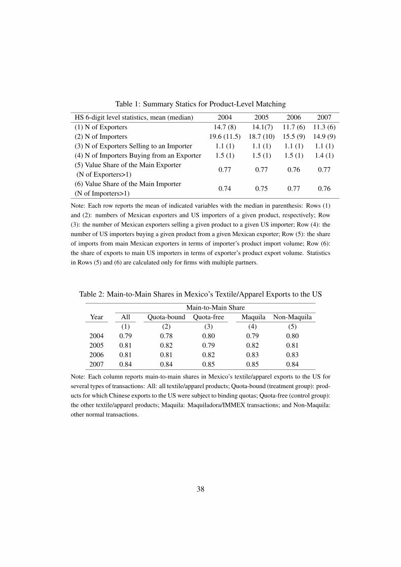
Table 1: Summary Statics for Product-Level Matching

HS 6-digit level statistics, mean (median) 2004 2005 2006 2007(1) N of Exporters 14.7 (8) 14.1(7) 11.7 (6) 11.3 (6)(2) N of Importers 19.6 (11.5) 18.7 (10) 15.5 (9) 14.9 (9)(3) N of Exporters Selling to an Importer 1.1 (1) 1.1 (1) 1.1 (1) 1.1 (1)(4) N of Importers Buying from an Exporter 1.5 (1) 1.5 (1) 1.5 (1) 1.4 (1)(5) Value Share of the Main Exporter

0.77 0.77 0.76 0.77(N of Exporters>1)(6) Value Share of the Main Importer

0.74 0.75 0.77 0.76(N of Importers>1)

Note: Each row reports the mean of indicated variables with the median in parenthesis: Rows (1)and (2): numbers of Mexican exporters and US importers of a given product, respectively; Row(3): the number of Mexican exporters selling a given product to a given US importer; Row (4): thenumber of US importers buying a given product from a given Mexican exporter; Row (5): the shareof imports from main Mexican exporters in terms of importer’s product import volume; Row (6):the share of exports to main US importers in terms of exporter’s product export volume. Statisticsin Rows (5) and (6) are calculated only for firms with multiple partners.

Table 2: Main-to-Main Shares in Mexico’s Textile/Apparel Exports to the US

Main-to-Main ShareYear All Quota-bound Quota-free Maquila Non-Maquila

(1) (2) (3) (4) (5)2004 0.79 0.78 0.80 0.79 0.802005 0.81 0.82 0.79 0.82 0.812006 0.81 0.81 0.82 0.83 0.832007 0.84 0.84 0.85 0.85 0.84

Note: Each column reports main-to-main shares in Mexico’s textile/apparel exports to the US forseveral types of transactions: All: all textile/apparel products; Quota-bound (treatment group): prod-ucts for which Chinese exports to the US were subject to binding quotas; Quota-free (control group):the other textile/apparel products; Maquila: Maquiladora/IMMEX transactions; and Non-Maquila:other normal transactions.

38

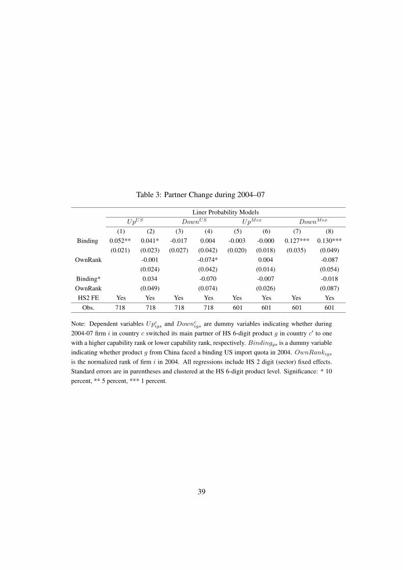
Table 3: Partner Change during 2004–07

Liner Probability ModelsUpUS DownUS UpMex DownMex

(1) (2) (3) (4) (5) (6) (7) (8)Binding 0.052** 0.041* -0.017 0.004 -0.003 -0.000 0.127*** 0.130***

(0.021) (0.023) (0.027) (0.042) (0.020) (0.018) (0.035) (0.049)OwnRank -0.001 -0.074* 0.004 -0.087

(0.024) (0.042) (0.014) (0.054)Binding* 0.034 -0.070 -0.007 -0.018OwnRank (0.049) (0.074) (0.026) (0.087)HS2 FE Yes Yes Yes Yes Yes Yes Yes Yes

Obs. 718 718 718 718 601 601 601 601

Note: Dependent variables Upcigs

and Downc

igs

are dummy variables indicating whether during2004-07 firm i in country c switched its main partner of HS 6-digit product g in country c0 to onewith a higher capability rank or lower capability rank, respectively. Binding

gs

is a dummy variableindicating whether product g from China faced a binding US import quota in 2004. OwnRank

igs

is the normalized rank of firm i in 2004. All regressions include HS 2 digit (sector) fixed effects.Standard errors are in parentheses and clustered at the HS 6-digit product level. Significance: * 10percent, ** 5 percent, *** 1 percent.

39

Table 4: Partner Change in Different Periods

A: Gradual Partner ChangesPartner Change in Different Periods: Linear Probability Models

UpUS DownMex

2004–06 2004–07 2004–08 2004–06 2004–07 2004–08(1) (2) (3) (4) (5) (6)

Binding 0.036** 0.052** 0.066** 0.056* 0.127*** 0.121***(0.015) (0.021) (0.027) (0.031) (0.035) (0.032)

HS2 FE Yes Yes Yes Yes Yes YesObs. 964 718 515 767 601 442

B: Placebo ChecksPartner Change in Different Periods: Linear Probability Models

UpUS DownMex

2007–11 2008–11 2009–11 2007–11 2008–11 2009–11(7) (8) (9) (10) (11) (12)

Binding -0.001 0.027** -0.000 -0.008 0.047 0.005(0.018) (0.011) (0.006) (0.036) (0.031) (0.020)

HS2 FE Yes Yes Yes Yes Yes YesObs. 449 575 747 393 499 655

Note: Dependent variables Upcigs

and Downc

igs

are dummy variables indicating whether duringthe period indicated by each column, firm i in country c switched its main partner of HS 6-digitproduct g in country c0 to one with a higher capability rank or lower capability rank, respectively.Binding

gs

is a dummy variable indicating whether product g from China faced a binding US importquota in 2004. All regressions include HS 2-digit (sector) fixed effects. Standard errors are shown inparentheses and clustered at the HS 6-digit product level. Significance: * 10 percent, ** 5 percent,*** 1 percent.

40

Table 5: Partner Change during 2004–07 with Additional Controls

A: HS 6-digit Product Level Controls: Linear Probability Models

Up

US

Down

Mex

(1) (2) (3) (4) (1) (2) (3) (4)

Binding 0.043** 0.44* 0.049** 0.042* 0.122*** 0.125*** 0.123*** 0.130***

(0.022) (0.022) (0.022) (0.024) (0.035) (0.037) (0.038) (0.037)

#Exporters 0.001*** 0.000

(0.000) (0.000)

#Importers 0.0003** 0.000

(0.0001) (0.000)

LnTotalTrade 0.002 0.002

(0.004) (0.007)

Product type Yes Yes

HS2 FE Yes Yes Yes Yes Yes Yes Yes Yes

Obs. 718 718 718 718 601 601 601 601

B: Firm-Product Level Controls: Linear Probability Models

Up

US

Down

Mex

(1) (2) (3) (4) (5) (6) (7) (8)

Binding 0.049** 0.053** 0.051** 0.049** 0.123*** 0.127*** 0.103*** 0.104***

(0.022) (0.022) (0.021) (0.019) (0.038) (0.035) (0.037) (0.034)

LnTrade 0.002 0.002

(0.004) (0.007)

Maquiladora -0.015 -0.025

(0.017) (0.024)

#Partners 0.007*** 0.036***

(0.002) (0.009)

US Intermediary 0.011 0.034

(0.013) (0.031)

HS2 FE Yes Yes Yes Yes Yes Yes Yes Yes

Obs. 718 718 718 629 601 601 601 489

Note: Dependent variables Up

c

igs

and Down

c

igs

are dummy variables indicating whether during 2004-07 firm i in country c

switched its main partner of HS 6-digit product g in country c

0 to one with a higher capability rank or lower capability rank,

respectively. Binding

gs

is a dummy variable indicating whether product g from China faced a binding US import quota

in 2004. #Exporters

g

and #Importers

g

are numbers of exporters and importers of product g in 2004, respectively.

LnTotalTrade

g

is the log of trade volume for product g in 2004. Product Types are a collection of dummy variables

indicating whether products are men’s, women’s, cotton, wool, or synthetic (man-made). LnTrade

ig

is the log of firm i’s

trade volume of product g in 2004. Maquiladora

ig

is the share of Maquiladora/IMMEX trade in firm i’s trade of product

g in 2004. #Partners

ig

is the number of firm i’s partner in product g in 2004. US Intermediary

ig

is a dummy variable

indicating whether US firm i or firm i’s US main partner is an intermediary firm. All regressions include HS 2-digit (sector)

fixed effects. Standard errors are shown in parentheses and clustered at the HS 6-digit product level. Significance: * 10

percent, ** 5 percent, *** 1 percent. 41

Table 6: Mexican Exporter’s Exit from the US market

Linear Probability ModelsExit

igsr

Period 1 2001–04 2002–04 2000–04Period 2 2004–07 2004–06 2004–08

(1) (2) (3) (4) (5) (6)Binding -0.040*** -0.035*** -0.037** -0.019 -0.019 -0.017

(�1) (0.014) (0.013) (0.015) (0.015) (0.013) (0.013)Binding 0.076*** 0.099*** 0.044** 0.064*** 0.032** 0.054***

*After (�2) (0.016) (0.020) (0.018) (0.021) (0.014) (0.02)After -0.361*** -0.331*** -0.454*** -0.427*** -0.262*** -0.184***(�3) (0.042) (0.069) (0.049) (0.081) (0.030) (0.068)

lnExport -0.058*** -0.059*** -0.078*** -0.076*** -0.045*** -0.046***(�4) (0.002) (0.002) (0.002) (0.002) (0.002) (0.002)

lnExport* 0.020*** 0.026*** 0.031*** 0.036*** 0.012*** 0.017***After (�5) (0.003) (0.003) (0.004) (0.003) (0.003) (0.002)Controls Yes Yes YesHS2 FE Yes Yes Yes Yes Yes Yes

Obs. 22625 22624 20655 20655 24474 24474Note: Dependent variable Exit

igsr

is a dummy variables indicating whether Mexican firm i stopsexporting product g to the US in period r. Binding

gs

is a dummy variable indicating whetherproduct g from China faced a binding US import quota in 2004. After

r

is a dummy variableindicating whether period r is after 2004. lnExport

igr

is the log of firm i’s export of product g inthe initial year of period r. Columns (2), (4) and (6) include the following control variables of theinitial year and their interactions with After

r

: share of Maquiladora/IMMEX trade in firm i’s tradeof product g in the initial year; log of trade volume for product g; number of exporters of product g;a collection of dummy variables indicating products types: whether products are men’s, women’s,cotton, wool, or synthetic (man-made). All regressions include HS 2-digit (sector) fixed effects.Standard errors are shown in parentheses and clustered at the HS 6-digit product level. Significance:* 10 percent, ** 5 percent, *** 1 percent.

42

Table 7: Alternative Capability Rankings

A: Partner Changes during 2004–07: Linear Probability ModelsUpUS DownUS

Baseline Total Trade Price Baseline Total Trade Price(1) (2) (3) (4) (5) (6)

Binding 0.052** 0.052** 0.047** -0.017 -0.017 0.006(0.021) (0.021) (0.018) (0.027) (0.027) (0.023)

HS2 FE Yes Yes Yes Yes Yes YesObs. 718 718 672 718 718 672

UpMex DownMex

Baseline Total Trade Price Baseline Total Trade Price(7) (8) (9) (10) (11) (12)

Binding -0.003 0.001 0.037 0.127*** 0.123*** 0.069**(0.020) (0.019) (0.031) (0.035) (0.035) (0.028)

HS2 FE Yes Yes Yes Yes Yes YesObs. 601 601 559 601 601 559

B: Old and New Partners 2004–07: OLSNew Partner Rank

US Importers Mexican ExportersBaseline Total Trade Price Baseline Total Trade Price

(13) (14) (15) (16) (17) (18)Old Partner 0.44*** 0.44*** 0.17* 0.74*** 0.68*** 0.47***

Rank (0.12) (0.13) (0.10) (0.13) (0.13) (0.12)Constant 0.24*** 0.24*** -0.44*** 0.25*** 0.25*** 0.30***

(0.05) (0.04) (0.06) (0.04) (0.04) (0.07)R2 0.13 0.15 0.04 0.24 0.21 0.14

Obs. 88 88 80 104 104 98

Note: Rankings are based on firm’s product trade with the main partner in 2004 in “Baseline”,firm’s product total trade in 2004 in “Total Trade”, and firm’s unit price of product in 2004 in“Price”. Significance: * 10 percent, ** 5 percent, *** 1 percent. (Panel A) Dependent variablesUpc

igs

and Downc

igs

are dummy variables indicating whether during 2004–07 firm i in country c

switched its main partner of HS 6-digit product g in country c0 to one with a higher capability rankor lower capability rank, respectively. Binding

gs

is a dummy variable indicating whether productg from China faced a binding US import quota in 2004. All regressions include HS 2-digit (sector)fixed effects. Standard errors are shown in parentheses and clustered at the HS 6-digit product level.(Panel B) Regressions are run for firm i in country c who switched their main partners of productg during 2004-07. The dependent variable NewPartnerRankc

ig

is the normalized rank of firm i’snew main partner of product g in 2007. OldPartnerRankc

ig

is the normalized rank of firm i’s oldmain partner of product g in 2004.

43

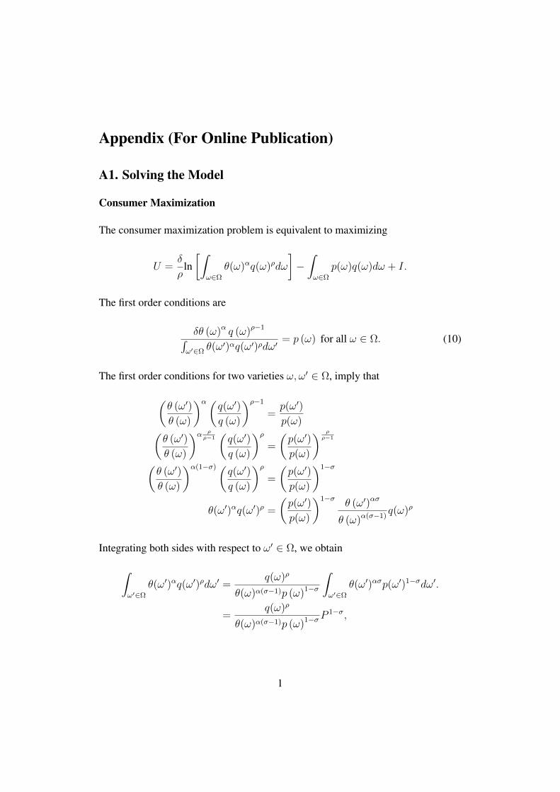
Appendix (For Online Publication)

A1. Solving the Model

Consumer Maximization

The consumer maximization problem is equivalent to maximizing

U =

�

⇢lnZ

!2⌦✓(!)↵q(!)⇢d!

��Z

!2⌦p(!)q(!)d! + I.

The first order conditions are

�✓ (!)↵ q (!)⇢�1

R!

02⌦ ✓(!0)

↵q(!0)

⇢d!0 = p (!) for all ! 2 ⌦. (10)

The first order conditions for two varieties !,!0 2 ⌦, imply that

✓✓ (!0

)

✓ (!)

◆↵

✓q(!0

)

q (!)

◆⇢�1

=

p(!0)

p(!)✓✓ (!0

)

✓ (!)

◆↵

⇢

⇢�1✓q(!0

)

q (!)

◆⇢

=

✓p(!0

)

p(!)

◆ ⇢

⇢�1

✓✓ (!0

)

✓ (!)

◆↵(1��)✓q(!0

)

q (!)

◆⇢

=

✓p(!0

)

p(!)

◆1��

✓(!0)

↵q(!0)

⇢

=

✓p(!0

)

p(!)

◆1�� ✓ (!0)

↵�

✓ (!)↵(��1)q(!)⇢

Integrating both sides with respect to !0 2 ⌦, we obtain

Z

!

02⌦✓(!0

)

↵q(!0)

⇢d!0=

q(!)⇢

✓(!)↵(��1)p (!)1��

Z

!

02⌦✓(!0

)

↵�p(!0)

1��d!0.

=

q(!)⇢

✓(!)↵(��1)p (!)1��

P 1��,

1

where P ⌘⇥R

!2⌦ p(!)1��✓ (!)↵� d!⇤1/(1��) is the price index. Substituting this

into (10), we obtain the demand function:

�✓ (!)↵ q (!)⇢�1

R!

02⌦ ✓(!0)

↵q(!0)

⇢d!0 = p (!)

�✓ (!)↵ q (!)⇢�1

✓(!)↵(��1)p (!)1��

q(!)⇢P 1��

!= p (!)

q(!) =�✓ (!)↵�

P 1��

p(!)��. (11)

Stage 2: Team profit maximization

Facing the demand function (11), teams choose prices under monopolistic compe-

tition. Let A ⌘ �

�

�⇢P

c

���1and � ⌘ ↵� � � (� � 1). Since a team with capability ✓

has marginal costs c✓� , it chooses the optimal price p(✓) = c✓

�

⇢

. The team’s output

q (✓), revenue R(✓), costs C(✓), and profits ⇧(✓) thus become

q (✓) = �P ��1⇣⇢c

⌘�

✓(↵��)�;

R(✓) = p(✓)q (✓)

= �

✓⇢P

c

◆��1

✓(↵��)�+�

= �A✓�;

C(✓) = c✓�q (✓) + f

=

�

⇢

✓⇢P

c

◆��1

✓(↵��)�+�

+ f

= (� � 1)A✓� + f ;

⇧ (✓) = R(✓)� C(✓) = A✓� � f.

2

Normalize � = 1. From the optimal price, the price index is

P =

Z

!2⌦p(!)1��✓ (!)↵� d!

�1/(1��)

=

c

⇢

Z

!2⌦✓ (!)� d!

�1/(1��)

=

c

⇢

Z

!2⌦✓ (!) d!

�1/(1��)

.

=

c

⇢⇥

1/(1��),

where ⇥ ⌘R!2⌦ ✓ (!) d! is the aggregate capability. Then, the index A becomes

A =

�

�

✓⇢P

c

◆��1

=

�

�⇥.

Stage 1

The mass of active final producers equals that of active suppliers:

MU

[1� F (xL

)] = (MM

+MC

) [1�G(yL

)]

This equation determine yL

(xL

) as an increasing function of xL

.

In Case C and Case I, a team with the lowest capability ✓L

consists of a final

producer with xL

and a supplier with yL

. This implies two properties. First, the

lowest capability ✓L

(xL

) = ✓ (xL

, yL

(xL

)) becomes an increasing fiction of xL

.

Second, this team’s profit is zero [⇧(✓L

) = ⇡x

(xL

) + ⇡y

(yL

) = 0], which implies

the team cutoff condition:

A✓L

= f.

3

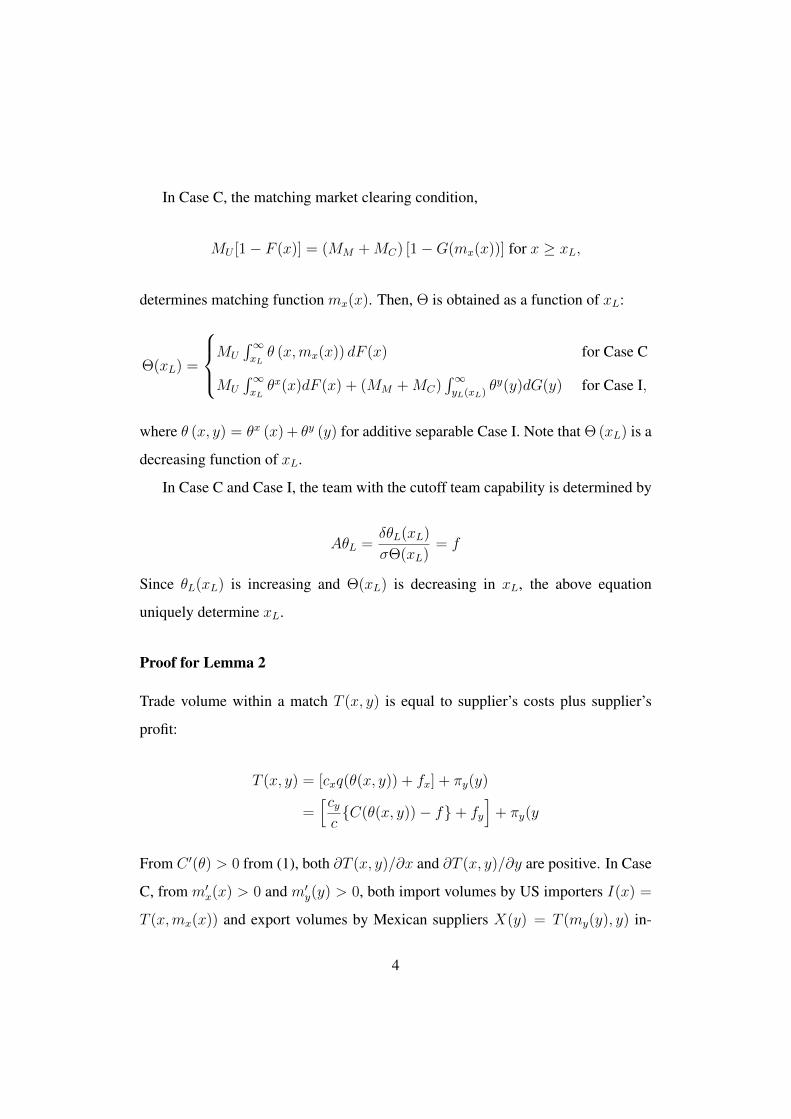
In Case C, the matching market clearing condition,

MU

[1� F (x)] = (MM

+MC

) [1�G(mx

(x))] for x � xL

,

determines matching function mx

(x). Then, ⇥ is obtained as a function of xL

:

⇥(xL

) =

8><

>:

MU

R1x

L

✓ (x,mx

(x)) dF (x) for Case C

MU

R1x

L

✓x(x)dF (x) + (MM

+MC

)

R1y

L

(xL

) ✓y

(y)dG(y) for Case I,

where ✓ (x, y) = ✓x (x) + ✓y (y) for additive separable Case I. Note that ⇥ (xL

) is a

decreasing function of xL

.

In Case C and Case I, the team with the cutoff team capability is determined by

A✓L

=

�✓L

(xL

)

�⇥(xL

)

= f

Since ✓L

(xL

) is increasing and ⇥(xL

) is decreasing in xL

, the above equation

uniquely determine xL

.

Proof for Lemma 2

Trade volume within a match T (x, y) is equal to supplier’s costs plus supplier’s

profit:

T (x, y) = [cx

q(✓(x, y)) + fx

] + ⇡y

(y)

=

hcy

c{C(✓(x, y))� f}+ f

y

i+ ⇡

y

(y

From C 0(✓) > 0 from (1), both @T (x, y)/@x and @T (x, y)/@y are positive. In Case

C, from m0x

(x) > 0 and m0y

(y) > 0, both import volumes by US importers I(x) =

T (x,mx

(x)) and export volumes by Mexican suppliers X(y) = T (my

(y), y) in-

4

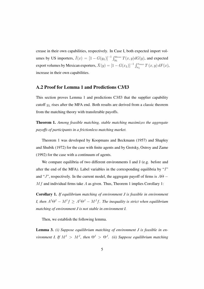
crease in their own capabilities, respectively. In Case I, both expected import vol-

umes by US importers, ¯I(x) = [1�G(yL

)]

�1 R y

max

y

L

T (x, y)dG(y), and expected

export volumes by Mexican exporters, ¯X(y) = [1�G(xL

)]

�1 R x

max

x

L

T (x, y) dF (x),

increase in their own capabilities.

A.2 Proof for Lemma 1 and Predictions C3/I3

This section proves Lemma 1 and predictions C3/I3 that the supplier capability

cutoff yL

rises after the MFA end. Both results are derived from a classic theorem

from the matching theory with transferable payoffs.

Theorem 1. Among feasible matching, stable matching maximizes the aggregate

payoffs of participants in a frictionless matching market.

Theorem 1 was developed by Koopmans and Beckmann (1957) and Shapley

and Shubik (1972) for the case with finite agents and by Gretsky, Ostroy and Zame

(1992) for the case with a continuum of agents.

We compare equilibria of two different environments I and J (e.g. before and

after the end of the MFA). Label variables in the corresponding equilibria by “I”

and “J”, respectively. In the current model, the aggregate payoff of firms is A⇥ �

Mf and individual firms take A as given. Thus, Theorem 1 implies Corollary 1:

Corollary 1. If equilibrium matching of environment J is feasible in environment

I, then AI

⇥

I � M If � AI

⇥

J � MJf . The inequality is strict when equilibrium

matching of environment J is not stable in environment I.

Then, we establish the following lemma.

Lemma 3. (i) Suppose equilibrium matching of environment J is feasible in en-

vironment I. If M I > MJ , then ⇥

I > ⇥

J . (ii) Suppose equilibrium matching

5

of environment J is feasible and not stable in environment I. If M I � MJ , then

⇥

I > ⇥

J .

Proof. (i) Since equilibrium matching of environment J is feasible in environment

I , AI

⇥

I �M If � AI

⇥

J �MJf from Corollary 1. Since M I > MJ , this implies

⇥

I > ⇥

J . (ii) Since equilibrium matching of environment J is feasible and not

stable in environment I , AI

⇥

I � M If > AI

⇥

J � MJf from Corollary 1. Since

M I � MJ , this implies ⇥I > ⇥

J

Proof for dyL

> 0 for Case C and Case I

Denote the environment after the MFA’s end as A-environment and the environ-

ment before the MFA’s end as B-environment. Label equilibrium variables of A-

environment by “A” and those of B-environment by “B”.

Lemma 4. yAL

> yBL

in Case C and Case I.

Proof. Suppose yAL

yBL

. This means that the mass of produced varieties and active

final producers increase: MA > MB and xA

L

< xB

L

. Since equilibrium matching

of B-environment is feasible in A-environment, Lemma 3 implies ⇥

A > ⇥

B. In

Case C and Case I, ✓L

= ✓(xL

, yL

), xA

L

< xB

L

and yAL

yBL

imply ✓AL

< ✓BL

. From

✓L

=

�f

�

⇥ in (6), we have ⇥

A < ⇥

B. This contradiction implies yAL

> yBL

.

Proof for Lemma 1

Denote the environment after the MFA’s end A-environment, the environment of

the no-rematching equilibrium as NR-environment, and the environment before the

MFA’s end as B-environment.

Claim 1. ⇥A

= ⇥

NR in Case I.

6

Proof. An equilibrium in the NR-environment agrees with an equilibrium in the

A-environment because no rematching occurs after the MFA’s end in Case I.

Claim 2. yAL

> yNR

L

> yBL

in Case C.

Proof. Suppose yNR

L

yBL

. This means xNR

L

< xB

L

and MNR > MB. Since

✓L

= ✓(xL

, yL

) holds in Case C and Case I, yNR

L

< yBL

and xNR

L

< xB

L

imply that

✓NR

L

< ✓BL

. From ✓L

=

�f

�

⇥ in (6), this means ⇥

NR < ⇥

B. Since equilibrium

matching in the B-environment is feasible in the NR-environment, Lemma 3 and

MNR > MB imply that ⇥NR > ⇥

B. This contradiction implies yNR

L

> yBL

.

Suppose yAL

yNR

L

. By an argument similar to that above, we have xA

L

xNR

L

and MA � MNR so that ✓AL

✓NR

L

, which implies ⇥A ⇥

NR. Since equilibrium

matching of the NR-environment is feasible and not stable in the A-environment,

Lemma 3 and MA � MNR imply ⇥

A > ⇥

NR. This contradiction implies yAL

>

yNR

L

.

Claim 3. ⇥A > ⇥

NR > ⇥

B in Case C and ⇥

NR > ⇥

B in Case I.

Proof. Suppose ⇥

NR ⇥

B, which implies that ✓NR ✓B from (6). Since

equilibrium matching in the B-environment is feasible and not stable in the NR-

environment, Lemma 3 implies MNR < MB. From M = MU

[1 � F (xL

)], this

means xNR

L

> xB

L

. In Case C and Case I, ✓L

= ✓(xL

, yL

), yNR

L

> yBL

from Claim 2,

and ✓NR

L

✓BL

imply xNR

L

< xB

L

. This contradiction implies ⇥NR > ⇥

B .

Consider Case C and suppose ⇥

A ⇥

NR, which implies ✓A ✓NR from (6).

Since equilibrium matching in the NR-environment is feasible and not stable in the

A-environment in Case C, Lemma 3 implies MA < MNR. From M = MU

[1 �

F (xL

)], this means xA

L

> xNR

L

. In Case C, ✓L

= ✓(xL

, yL

), yAL

> yNR

L

from Claim

3, and ✓AL

✓NR

L

imply xA

L

< xNR

L

. This contradiction implies ⇥A > ⇥

NR.

From P = c/�⇢⇥1/(��1)

�, Claims 1–3 prove Lemma 1.

7

A.3 Negative Assortative Matching

Solving the Model

In Case S, the market clearing condition becomes

MU

[1� F (x)] = (MM

+MC

) [G (mx

(x))�G(yL

)] for all x � xL

. (12)

The left hand side is the mass of final producers with higher capability than x and

the right hand side is the mass of suppliers with lower capability than mx

(x).

An equilibrium is obtained as follows. The condition (12) determines mx

(x)

for all x � xL

. Then, ⇥ is obtained as a decreasing function of xL

:

⇥(xL

) = MU

Zx

max

x

L

✓ (x,mx

(x)) dF (x).

A supplier with ymax

matches with a final producer with xL

and receives whole

team profits because ⇡x

(xL

) = 0:

⇡y

(ymax

) = ⇧(✓(xL

, ymax

)) = A✓ (xL

, ymax

)� f.

The profit of supplier with ymax

is obtained by integrating the first order condition:

⇡y

(ymax

) =

Zy

max

y

L

⇡0y

(y)dy = A

Zy

max

y

L

✓2(my

(t), t)dt.

From A =

�

�⇥ and yL

= mx

(xmax

), the above two equations imply

A✓ (xL

, ymax

)� f = A

Zy

max

m

x

(xmax

)

✓2(my

(t), t)dt

�

�⇥(xL

)

✓ (x

L

, ymax

)�Z

y

max

m

x

(xmax

)

✓2(my

(t), t)dt

�= f. (13)

8

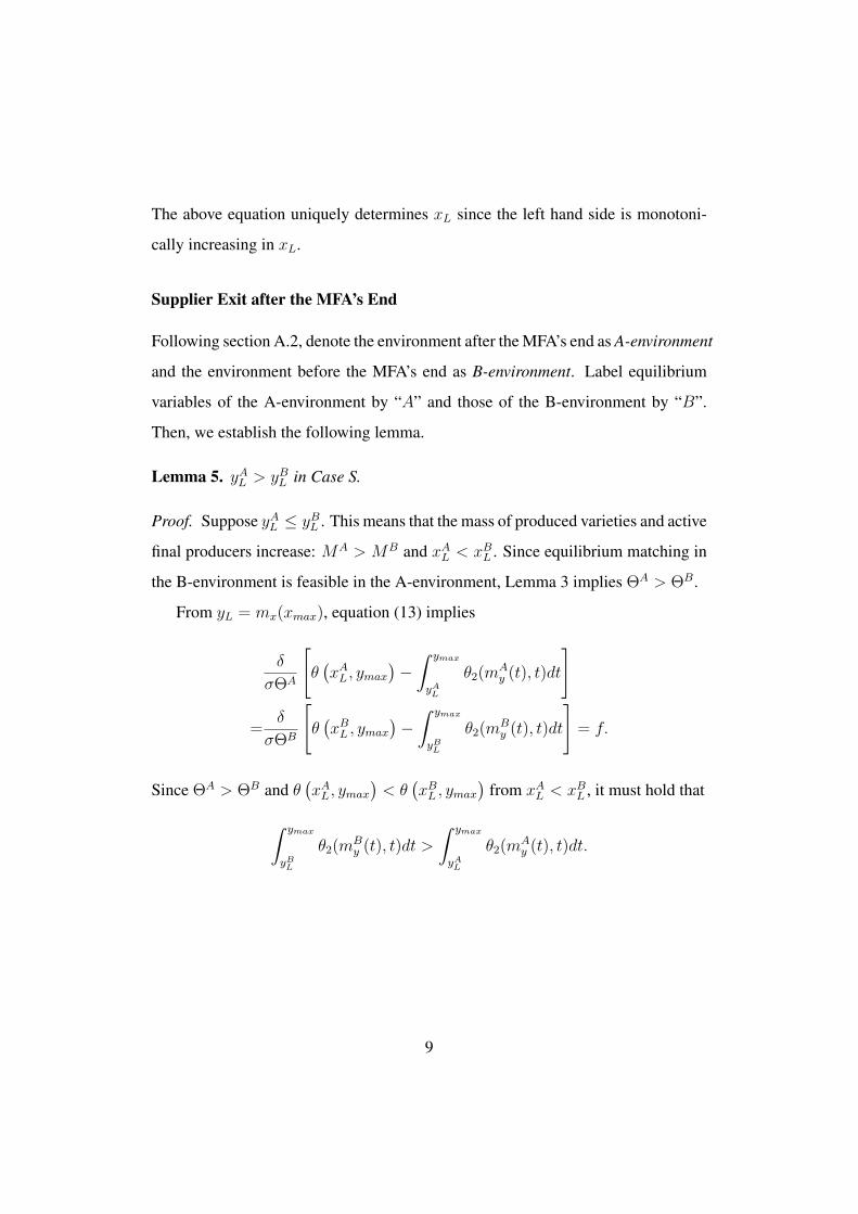
The above equation uniquely determines xL

since the left hand side is monotoni-

cally increasing in xL

.

Supplier Exit after the MFA’s End

Following section A.2, denote the environment after the MFA’s end as A-environment

and the environment before the MFA’s end as B-environment. Label equilibrium

variables of the A-environment by “A” and those of the B-environment by “B”.

Then, we establish the following lemma.

Lemma 5. yAL

> yBL

in Case S.

Proof. Suppose yAL

yBL

. This means that the mass of produced varieties and active

final producers increase: MA > MB and xA

L

< xB

L

. Since equilibrium matching in

the B-environment is feasible in the A-environment, Lemma 3 implies ⇥A > ⇥

B.

From yL

= mx

(xmax

), equation (13) implies

�

�⇥A

"✓�xA

L

, ymax

��Z

y

max

y

A

L

✓2(mA

y

(t), t)dt

#

=

�

�⇥B

"✓�xB

L

, ymax

��Z

y

max

y

B

L

✓2(mB

y

(t), t)dt

#= f.

Since ⇥

A > ⇥

B and ✓�xA

L

, ymax

�< ✓

�xB

L

, ymax

�from xA

L

< xB

L

, it must hold that

Zy

max

y

B

L

✓2(mB

y

(t), t)dt >

Zy

max

y

A

L

✓2(mA

y

(t), t)dt.

9

Since yAL

yBL

, this implies

Zy

max

y

B

L

Zm

B

y

(t)

m

A

y

(t)

✓12(z, t)dzdt =

Zy

max

y

B

L

⇥✓2(m

B

y

(t), t)� ✓2(mA

y

(t), t)⇤dt

=

Zy

max

y

B

L

✓2(mB

y

(t), t)dt�Z

y

max

y

B

L

✓2(mA

y

(t), t)dt

�Z

y

max

y

B

L

✓2(mB

y

(t), t)dt�Z

y

max

y

A

L

✓2(mA

y

(t), t)dt

> 0. (14)

On the other hands, the matching market clearing condition implies for all y �

yBL

, it must hold that

MU

⇥1�G(mA

y

(y))⇤=

�M

M

+MA

C

� ⇥G(y)�G(yA

L

)

⇤,

MU

⇥1�G(mB

y

(y))⇤=

�M

M

+MB

C

� ⇥G(y)�G(yB

L

)

⇤.

Taking the difference of both sides, we obtain for all y � yBL

,

MU

⇥G(mB

y

(y))�G(mA

y

(y))⇤=

�M

M

+MA

C

� ⇥G(y)�G(yA

L

)

⇤

��M

M

+MB

C

� ⇥G(y)�G(yB

L

)

⇤> 0

since MA

C

> MB

C

and G(yAL

) G(yBL

) from yAL

yBL

. Thus, we have mB

y

(y) >

mA

y

(y) for all y � yBL

. From ✓12 < 0, this implies

Zy

max

y

B

L

Zm

B

y

(t)

m

A

y

(t)

✓12(z, t)dzdt < 0,

which contradicts with (14).

10

Partner Changes after the MFA’s End

Assumption 1. If the mass of Chinese suppliers MC

increases, then the total mass

of suppliers in the US (MC

+MM

) [1�G(yL

)] increases.

Under this assumption, the capability cutoff for importing xL

falls. The follow-

ing lemma shows the direction of US importers’ partner changes is heterogeneous.

Lemma 6. Under Assumption 1, there exists a threshold capability x̃ 2 (xL

, xmax

)

such that when the mass of Chinese suppliers increase, continuing US final pro-

ducers with x > x̃ switch Mexican partner to one with higher capability (partner

upgrading), while continuing US final producers with x < x̃ switch Mexican part-

ner to one with lower capability (partner downgrading).

Proof. Totally differentiating (12), we obtain the partner change of importers with

capability x:

dmx

(x) =�(x)

g(mx

(x)),�(x) ⌘ g(y

L

)dyL

� G (mx

(x))�G(yL

)

(MM

+MC

)

dMC

. (15)

Since dyL

> 0, dMC

> 0, and m0x

(x) < 0, �(x) is increasing in x and �(xmax

) =

g(yL

)dyL

> 0 since yL

= mx

(xmax

). Since Assumption 1 implies

d (MC

+MM

) [1�G(yL

)] = [1�G(yL

)]dMC

� (MC

+MM

) g(yL

)dyL

> 0,

�(xL

) ⌘ g(yL

)dyL

� 1�G(yL

)(M

M

+M

C

)dMC

< 0. Since �(x) is continuous, there exists

x̃ 2 (xL

, xmax

) such that �(x) > 0 for x > x̃ and �(x) < 0 for x < x̃.

To understand the intuition for this lemma, it is useful to consider how firms with

maximum capabilities change partners. Suppose xL

falls from xB

L

to xA

L

and yL

rises

from yBL

to yAL

. Since final producers with maximum capability xmax

always match

11

with suppliers who have the cutoff capability yL

, they upgrade partner suppliers

with yBL

to yAL

. On the other hand, since suppliers with maximum capability ymax

always match with final producers with the cutoff capability xL

, they downgrade

final producers from xB

L

to xA

L

. This in turn means that final producers with xB

L

downgrade partner suppliers. Since a matching function is continuous, there is a

threshold x̂ of the lemma.

A.4 Data Construction

Customs transaction data Our primary data set is a Mexican customs transaction

data set for Mexican textile/apparel exports to the US. The data set is created from

the administrative records held on every transaction crossing the Mexico–US bor-

der from June 2004 to December 2011. The Mexican customs agency requires both

individuals and firms who ship goods across the border to submit a customs form

(pedimento aduanal in Spanish) that must be prepared by an authorized agent. The

form contains information on (1) date of clearing customs; (2) total value of ship-

ment (in US dollars); (3) 8-digit HS product code (we use from HS50 to HS63); (4)

quantity and unit; (5) name, address, and tax identification number of the Mexican

exporter; (6) name, address, and tax identification number (employment identifica-

tion number, EIN) of the US importer; (7) an indicator of a duty free processing

reexport program (the Maquiladora/IMMEX program); and other information.

Assign firm IDs We assigned identification numbers to both Mexican exporters

and US importers (exporter-ID and importer-ID) throughout the data set. It is

straightforward to assign exporter-IDs for Mexican exporters since the Mexican tax

number uniquely identifies each Mexican firm. However, a challenge arises in as-

signing importer-IDs for US firms. It is known that one US firm often has multiple

12

names, addresses, and EINs. This happens because a firm sometimes uses multiple

names or changes names, owns multiple plants, or changes tax numbers. There-

fore, simply matching firms by one of three linking variables (names, addresses,

and EINs) would wrongly assign more than one ID to one US buyer and would

result in overestimating the number of US buyers for each Mexican exporter.

We therefore used a series of methods developed in record-linkage research for

data cleaning to assign importer-ID.41 First, as the focus of our study is firm-to-

firm matching, we dropped transactions for which exporters were individuals and

courier companies (e.g., FedEx, UPS, etc.). Second, we standardized the format

of addresses using the software, ZP4, which received a quality certification of ad-

dress cleaning (CASS certification) from the United States Postal Services. Third,

we remove generic words in company names that did not help identify a particu-

lar company such as legal terms (e.g., Co., Ltd., etc.). Fourth, we prepared lists of

fictitious names, previous names and name abbreviations, a list of addresses of com-

pany branches, and a list of EINs from data on company information, using Orbis

by Bureau van Dijk, which covers 20 millions company branches, subsidiaries, and

headquarters in the US.42 Fifth, for each HS 2-digit industry, we matched names

within customs data and names between customs data and name lists from Orbis

mentioned above. In conducting our matching, we used fuzzy matching techniques

allowing small typographical errors and abbreviations.43 To increase the accuracy41An excellent textbook for record linkage is Herzog, Scheuren, and Winkler (2007). In additon,

a webpage of “Virtual RDC@Cornell” (http://www2.vrdc.cornell.edu/news/) by Cornell Universityis also a great source of information on data cleaning. We particularly benefitted from lecture slideson “Record Linkage” by John Abowd and Lars Vilhuber.

42The primary source of US company information in Orbis (2012 version) is Dun&Bradstreet. Weused Orbis information for manufacturing firms and intermediary firms (wholesalers and retailers)due to the capacity of our workstation.

43The two names compared are “fuzzy matched” if one of the followings is satisfied: (1) they areclose to each other in terms of the Jaro-Winkler metric, which is available in the Record Linkagepackage of R; (2) they agree on the number of the first n letters; (3) the longer of the two namesincludes the shorter one.

13

of fuzzy matching, we removed words commonly appearing in the industry (e.g.,

“apparel”) from the two names compared if the word appears in both names. Also

we do not apply fuzzy matching techniques to very short names. Sixth, we con-

ducted similar matches for addresses and EINs. For addresses, we also use fuzzy

matching techniques for street and city name matching.

From these operations, we obtain matched pairs of names, addresses and EINs.

Then, using these matched relations and the network theory software (the igraph

package of R), we created clusters of information (names, addresses, and EINs) in

which one cluster identifies one firm. We identified a cluster utilizing the following

general rule. Each entry in a cluster matches with some other entries in the cluster

either by EIN or by both names and addresses. After automatically creating clus-

ters, we manually checked them and separated entries that should not have been

matched. Finally, we assigned importer-IDs to each cluster.

Data Cleaning Some information was dropped from the dataset. First, we dropped

exporters who are individuals or courier companies (e.g., FedEx, UPS, etc.) because

we focus on firm to firm matching. Second, as the dataset contains information only

from June to December for 2004, we dropped observations from January to May

for other years to make each year’s information comparable. We conducted our

main analysis (Tables 2 and 3) without conducting these two operations and still

obtained similar results. Third, we dropped one product (HS570210) where the

number of importers unreasonably fluctuates, suggesting low data quality.44 Fi-

nally, we dropped transactions by exporters who do not report importer information

for most transactions. For a given HS 6-digit product and a given year, we dropped

an exporter from the final data if the total value of transactions without importer44The number of US importers were 5 in 2004, 4 in 2005, 254 in 2006, 532 in 2007, 3 in 2008

and 123 in 2009.

14

information constituted more than 20% of the exporter’s annual export value. This

resulted in dropping approximately 30–40% of exporters and 60–70% of export

values. These dropped exporters are mostly Maquiladora/IMMEX exporters.

A5. Variable Construction

Product-Level Variables Dummy variable Bindinggs

equals one if Chinese ex-

ports of product g to the US faced a binding quota in 2004, which we construct from

Brambilla et al. (2010), who constructed an indicator for binding quotas on Chinese

exports to the US for each HS 10-digit category. Since HS product categories for

Mexico and the US are the same only up to the first 6 digits, we aggregated their

indicator up to the HS 6-digit level. A quota is defined as binding if the fill rate, i.e.,

realized import value over the quota value, is greater than 0.8. Our results are robust

to choice of other cut-offs. We constructed our indicator as follows. Let xm

j2004 be

US imports of HS 10-digit product j from Mexico in 2004. Let g be a HS 6-digit

product and J(g) be the set of US HS 10-digit products in category g. Thereafter,

we constructed a dummy variable indicating whether Chinese exports of HS 6-digit

product g to the US faced binding quotas in 2004 as:

Bindingg

= I

(Pj2J(g) x

m

j2004I{quota on j was binding in 2004}P

j2J(g) xm

j2004

� 0.5

),

(16)

where the indicator function I{X} = 1 if X is true and I{X} = 0 otherwise. We

chose the cut-off value as 0.5 but the choice of this cut-off is unlikely to affect the

results because most of values inside the indicator function are close to either one

or zero.

Product type dummies “Men”, “Women”, “Wool”, “Cotton”, and “Manmade”

equal one if the description of the HS 6 product clasification includes the words

15

“men”, “women”, “wool”, “cotton”, or “manmade”, respectively. #Exportersgs

is the number of exporters of product g in 2004, #Importersgs

is the number

of importers of product g in 2004, and TotalTradegs

is the total trade volume of

product g in 2004 .

Firm-Level and Firm-Product-Level Characteristics OwnRankigs

is firm’s nor-

malized rank in terms of trade volume in product g that falls in [0, 1]. For exporter

i, define ExRankigs

as firm i’s rank based on its trade volume of product g with

the main partner in 2004 among exporters of product g in 2004 (small ExRankigs

means large export volume). Similarly, define ImRankigs

for importers. Then, the

exporter’s normalized rank is OwnRankigs

= (ExRankigs

� 1) / (#Exportersgs

� 1)

so that OwnRankigs

falls in [0, 1]. OwnRankigs

becomes zero for the highest

ranked (largest) exporter becomes and one for the lowest ranked (smallest) exporter.

Similarly, for the importers, OwnRankigs

= (ImRankigs

� 1) / (#Importersgs

� 1).

Dummy variable NorthernStateigs

equals one if exporter i of product g is

located in one of the northern states of Mexico: Baja California, Sonora, Chihuahua,

Coahuila, Nuevo Leon and Tamaulipas. Maquiladoraigs

is the ratio of firm i’s

Maquiladora trade volume of product g over the firm’s total trade volume of product

g in 2004. lnTotalTradegs

is the log of total trade volume for product g in 2004.

Dummy variable US Intermediaryigs

equals one either if firm i is a US in-

termediary firm or if firm i is a Mexican exporter and its US main partner is an

intermediary firm. US intermediary firms are identified as follows. One US im-

porter is typically matched with several records of US firms in Orbis data since

Orbis data record branches and subsidiaries as distinct records. The US importer is

identified as an intermediary firm if one of matched records report retail or whole-

saling as its main industry and if none of matched records report manufacturing as

its main industry.

16

Other firm-level characteristics include the following. #Partnersigs

is the

number of partners with whom firm i trade in product g in 2004. MainPartner Shareigs

is the ratio of firm i’s trade volume of product g with the main partner over firm i’s

total trade volume of product g in 2004. lnTradeigs

is the log of firm i’s total trade

volume of product g in 2004.

A6. Main-to-Main Share at Product Level

Two panels in Figure 5 draw the distribution of main-to-main shares across product-

year combinations. A histogram in the left panel strikingly shows that main-to-main

shares exceed 0.9 for most combinations with the median 0.97 and 25th percentile

0.86. The right panel in Figure 5 plots main-to-main shares against the maximum

of the number of importers (nm

) and exporters (nx

), max{nm

, nx

}. This exercise is

motivated by the love of variety model with symmetric firms that predicts main-to-

main share will equal 1/max{nm

, nx

}. An estimated Lowess curve is above 0.80

and almost horizontal, which implies that main-to-main share is not related with

the total number of firms. Figure 5 remains very similar when the horizontal axis

expresses either nm

or nx

.

17

Figure 5: Main-to-Main Shares for HS 6-Digit Textile/Apparel Products

0.1

.2.3

.4.5

Frac

tion

.2 .4 .6 .8 1

Main to main share by product

.2.4

.6.8

1M

ain

to m

ain

shar

e

0 50 100 150 200 250Max(Number of importers, Number of exporters)

Main to main share Lowess

Main to main share and number of firms

Note: Both panels draw main-to-main share across product-year combinations of HS 6-digit tex-tile/apparel products and years 2004-2007. The left panel presents a histogram. The right panelplots main-to-main shares against the maximum of the numbers of exporters and importers.

A7. Summary Statistics and Treatment Control Group Compar-

ison

Table 8 provides summary statics of product-level characteristics. Column (1) re-

ports means and standard deviations of each product level characteristics for the

control group, with the number of observations in Column (2). Columns (3) and (4)

report the difference in each characteristic between treatment and control groups.

We regress each characteristic of product g on the treatment dummy Bindinggs

and

report the OLS coefficient b of the dummy in Column (3). Column (4) reports the

OLS coefficient b of the dummy from a similar regression with HS 2-digit fixed

effects, which captures the difference between the two groups within the same HS

2-digit sector. Column (5) reports the number of observations for the regressions

for Columns (3) and (4). Though a simple comparison in Column (3) shows that

the two groups differ in many characteristics, with HS 2-digit fixed effects the dif-

ference becomes smaller and even insignificant for many characteristics, as shown

in Column (4).

18

By the nature of the MFA’s end, the control group consists of products that were

already liberalized before 2002. Thus, the treatment group, which was protected in

2004, show more exporters and importers and greater trade volume then the control

group.

Table 9 reports similar summary statistics for importer-product level character-

istics. Even with HS 2-digit fixed effects, the treatment group shows more trade

volume and a higher share of processing trade (Maquiladora/IMMEX).

Table 10 reports similar summary statistics for exporter-product level charac-

teristics. Even with HS 2-digit fixed effects, Mexican exporters in the treatment

group export more with more partners, have a higher share of processing trade

(Maquiladora/IMMEX) and are less likely to trade with intermediary firms.

19

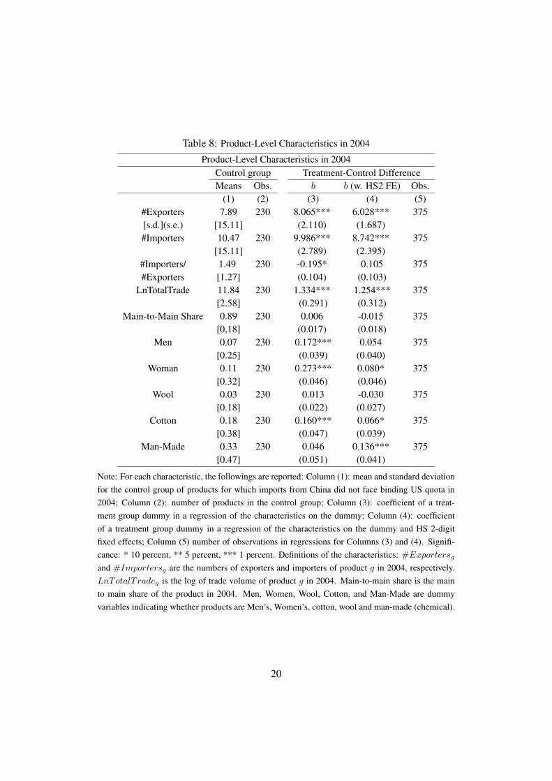
Table 8: Product-Level Characteristics in 2004

Product-Level Characteristics in 2004Control group Treatment-Control DifferenceMeans Obs. b b (w. HS2 FE) Obs.

(1) (2) (3) (4) (5)#Exporters 7.89 230 8.065*** 6.028*** 375[s.d.](s.e.) [15.11] (2.110) (1.687)#Importers 10.47 230 9.986*** 8.742*** 375

[15.11] (2.789) (2.395)#Importers/ 1.49 230 -0.195* 0.105 375#Exporters [1.27] (0.104) (0.103)

LnTotalTrade 11.84 230 1.334*** 1.254*** 375[2.58] (0.291) (0.312)

Main-to-Main Share 0.89 230 0.006 -0.015 375[0,18] (0.017) (0.018)

Men 0.07 230 0.172*** 0.054 375[0.25] (0.039) (0.040)

Woman 0.11 230 0.273*** 0.080* 375[0.32] (0.046) (0.046)

Wool 0.03 230 0.013 -0.030 375[0.18] (0.022) (0.027)

Cotton 0.18 230 0.160*** 0.066* 375[0.38] (0.047) (0.039)

Man-Made 0.33 230 0.046 0.136*** 375[0.47] (0.051) (0.041)

Note: For each characteristic, the followings are reported: Column (1): mean and standard deviationfor the control group of products for which imports from China did not face binding US quota in2004; Column (2): number of products in the control group; Column (3): coefficient of a treat-ment group dummy in a regression of the characteristics on the dummy; Column (4): coefficientof a treatment group dummy in a regression of the characteristics on the dummy and HS 2-digitfixed effects; Column (5) number of observations in regressions for Columns (3) and (4). Signifi-cance: * 10 percent, ** 5 percent, *** 1 percent. Definitions of the characteristics: #Exporters

g

and #Importersg

are the numbers of exporters and importers of product g in 2004, respectively.LnTotalTrade

g

is the log of trade volume of product g in 2004. Main-to-main share is the mainto main share of the product in 2004. Men, Women, Wool, Cotton, and Man-Made are dummyvariables indicating whether products are Men’s, Women’s, cotton, wool and man-made (chemical).

20

Table 9: Importer-Product Level Characteristics in 2004

Importer-Product Level Characteristics in 2004Own Characteristics

Control group Treatment-Control Differencemeans Obs. b b (w. HS2 FE) Obs.

(1) (2) (3) (4) (5)US Intermediary 0.33 1570 -0.002 -0.033 3429

[s.d.](s.e.) [0.47] (0.016) (0.022)LnTrade 7.86 2408 0.785*** 0.571*** 5374

[3.24] (0.093) (0.119)N of Partners 1.12 2408 0.013 0.012 5374

[1.32] (0.027) (0.034)Maquiladora 0.25 2408 0.198*** 0.130*** 5374

[0.42] (0.013) (0.016)Main Partner Share 0.76 124 0.012 -0.011 396

[0.21] (0.020) (0.027)Main Partner’s Characteristics

Control group Treatment-Control DifferenceMean Obs. b b (w. HS2 FE) Obs.

Northern State 0.15 2408 -0.027*** 0.002 5374[s.d.](s.e.) [0.36] (0.010) (0.012)

Note: For each characteristic, the followings are reported: Column (1): mean and standard deviationfor the control group of products for which imports from China did not face binding US quota in2004; Column (2): number of products in the control group; Column (3): coefficient of a treatmentgroup dummy in a regression of the characteristics on the dummy; Column (4): coefficient of atreatment group dummy in a regression of the characteristics on the dummy and HS 2-digit fixedeffects; Column (5): number of observations in regressions for Columns (3) and (4). Significance:* 10 percent, ** 5 percent, *** 1 percent. Definitions of the characteristics: LnTrade

ig

is the logof firm i’s trade volume of product g in 2004. Maquiladora

ig

is the share of Maquiladora/IMMEXtrade in firm i’s trade of product g in 2004. #Partners

ig

is the number of firm i’s partner in productg in 2004. US Intermediary

i

is a dummy variable indicating whether US importer or US mainpartner is an intermediary firm. NorthernState

ig

is a dummy indicating whether firm i’s Mexicanmain partner of product g is located in a northern state in Mexico.

21

Table 10: Exporter-Product Level Characteristics in 2004

Exporter-Product Level Characteristics in 2004Own Characteristics

Control group Treatment-Control DifferenceMean Obs. b b (w. HS2 FE) Obs.

(1) (2) (3) (4) (5)Maquiladora 0.33 1818 0.122*** 0.093*** 4131

[s.d.](s.e.) [0.46] (0.015) (0.019)Northern State 0.24 1818 -0.103*** 0.002 4131

Dummies [0.43] (0.012) (0.015)LnTrade 7.60 1818 1.562*** 0.963*** 4131

[3.52] (0.109) (0.139)N of Partners 1.5 1818 -0.036 0.213*** 4131

[2.01] (0.056) (0.072)Main Partner Share 0.73 296 0.018 -0.014 724

[0.21] (0.016) (0.022)Main Partner’s Characteristics

Control group Treatment-Control DifferenceMean Obs. b b (w. HS2 FE) Obs.

US Intermediary 0.31 1219 0.020 -0.053** 2833[s.d.](s.e.) [0.46] (0.018) (-0.024)

Note: For each characteristic, the followings are reported: Column (1): mean and standard deviationfor the control group of products for which imports from China did not face binding US quota in2004; Column (2): number of products in the control group; Column (3): coefficient of a treatmentgroup dummy in a regression of the characteristics on the dummy; Column (4): coefficient of atreatment group dummy in a regression of the characteristics on the dummy and HS 2-digit fixedeffects; Column (5): number of observations in regressions for Columns (3) and (4). Significance:* 10 percent, ** 5 percent, *** 1 percent. Definitions of the characteristics: LnTrade

ig

is the logof firm i’s trade volume of product g in 2004. Maquiladora

ig

is the share of Maquiladora/IMMEXtrade in firm i’s trade of product g in 2004. #Partners

ig

is the number of firm i’s partner in productg in 2004. US Intermediary

ig

is a dummy variable indicating whether firm i’s US main partner ofproduct g is an intermediary firm. NorthernState

i

is a dummy indicating whether firm i is locatedin a northern state in Mexico.

22

A.8. Alternative Explanations

This section discusses alternative hypotheses for our findings and presents addi-

tional evidence showing these do not fully explain our results.

Negative Assortative Matching (NAM) Appendix A.3 shows that Case S is dif-

ferent from Case C and Case I in two aspects. First, firm’s trade volume may not

be monotonically increasing in capability. The import volume of US importers

with capability x, I(x), and export volume of Mexican exporters with capability y,

X(y), satisfy X(mx

(x)) = I(x). Since X 0(m

x

(x))m0x

(x) = I 0(x) and m0x

(x) < 0,

then I 0(x) and X 0(y = m

x

(x)) must have the opposite signs. Thus, it is impossi-

ble that the trade ranking agrees with true capability ranking both for exporters and

importers. Second, the MFA’s end is likely to increase the mass of total suppliers in

the US. In this case, the direction of partner change depends on the firm’s capabil-

ity. A threshold capability x̃ exists such that US importers with x > x̃ upgrade their

partners, while those with x < x̃ downgrade their partners. With these two com-

plications, it is theoretically possible yet unlikely that NAM explains the observed

systematic relationships between rematching and trade ranking.

Segment Switching Another explanation for partner changes is the “segment

switching” theory inspired by Holmes and Stevens (2014). Even one HS 6-digit

product category may have two different segments. One, a “standardized” segment,

is produced on a large scale and sold with low markups, while the other, a “cus-

tom” segment, is produced on a small scale but sold with high markups. Suppose

that large US importers produce “standardized” products while small US importers

produce “custom” products. Further suppose that Chinese exporters enter mainly in

“standardized” products and that Mexican exporters switched from “standardized”

to “custom” products to escape competition. This change might be observed as

23

Mexican exporters’ partner downgrading and US importers’ partner upgrading.

If this hypothesis mainly explains our findings, small firms and large firms

should respond to the end of the MFA in heterogeneous ways. As small “cus-

tom” US importers should become more attractive to Mexican exporters and able

to match to more capable Mexican exporters, small US importers should upgrade

partners more frequently than large US importers. However, Table 3 shows that

both small and large US importers upgrade partners in a similar way.

Furthermore, Table 11 examines whether imports by initially small “custom”

US importers show higher growth rates than those by large “standardized” US im-

porters. The hypothesis predicts predicts such heterogeneous growth should be

stronger in the treatment group than in the control group. To test this hypothesis,

Column (1) regresses US importer’s import growth on the binding dummy and the

firm’s own rank and Column (2) adds the interaction of the firm’s own rank with the

binding dummy. Note that a small OwnRank indicates a large size. A positive co-

efficient on Own Rank in Row (1) shows small-sized US importers grow more than

large US importers. However, a small and insignificant interaction term in Column

(2) shows this heterogeneous effect is almost the same between the treatment and

control groups, which is inconsistent with the segment-switching hypothesis.

Production Capacity Another hypothesis posits that firm’s trade volume mainly

reflects the size of Mexican supplier’s production capacity instead of productivity

and quality. Since production capacity can be regarded as an element of firm’s

capability, this hypothesis is still consistent with PAM by capability.

Furthermore, the mere demand for production capacity is unlikely to be the

main reason for the observed partner upgrading. Columns (3) and (4) in Table 11

tests the production capacity hypothesis. If US importers in the treatment group

switch to Mexican exporters with greater preshock exports mainly to seek greater

24

production capacity, we should see the following two patterns. First, US importers

in the treatment group should show greater import growth than those in the control

group. Second, the difference should be driven by US importers in the treatment

group who actually upgrade partners. To test these two predictions, Column (3)

regresses US importer’s import growth on the binding dummy and Column (4) adds

the partner upgrading dummy and its interaction with the binding dummy. Columns

(3) and (4) show that the import growth of US importers is not correlated with

whether firms belong to the treatment group or whether the firms actually upgraded

partners. Thus, the demand for production capacity alone is unlikely to explain the

observed partner upgrading.

25

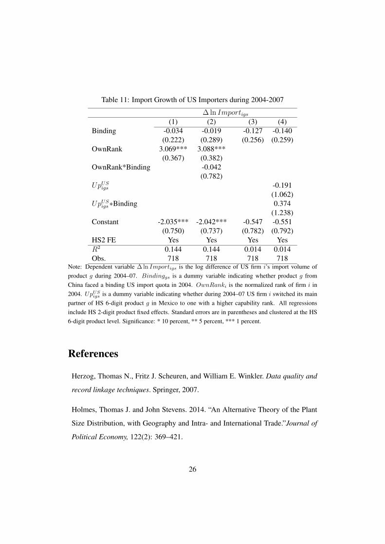
Table 11: Import Growth of US Importers during 2004-2007

� ln Importigs

(1) (2) (3) (4)Binding -0.034 -0.019 -0.127 -0.140

(0.222) (0.289) (0.256) (0.259)OwnRank 3.069*** 3.088***

(0.367) (0.382)OwnRank*Binding -0.042

(0.782)UpUS

igs

-0.191(1.062)

UpUS

igs

⇤Binding 0.374(1.238)

Constant -2.035*** -2.042*** -0.547 -0.551(0.750) (0.737) (0.782) (0.792)

HS2 FE Yes Yes Yes YesR2 0.144 0.144 0.014 0.014Obs. 718 718 718 718

Note: Dependent variable � ln Importigs

is the log difference of US firm i’s import volume ofproduct g during 2004–07. Binding

gs

is a dummy variable indicating whether product g fromChina faced a binding US import quota in 2004. OwnRank

i

is the normalized rank of firm i in2004. UpUS

igs

is a dummy variable indicating whether during 2004–07 US firm i switched its mainpartner of HS 6-digit product g in Mexico to one with a higher capability rank. All regressionsinclude HS 2-digit product fixed effects. Standard errors are in parentheses and clustered at the HS6-digit product level. Significance: * 10 percent, ** 5 percent, *** 1 percent.

References

Herzog, Thomas N., Fritz J. Scheuren, and William E. Winkler. Data quality and

record linkage techniques. Springer, 2007.

Holmes, Thomas J. and John Stevens. 2014. “An Alternative Theory of the Plant

Size Distribution, with Geography and Intra- and International Trade.”Journal of

Political Economy, 122(2): 369–421.

26