Andre Koch Torres Assis and

Julio Akashi Hernandes

The Electric Force of a Current

Th

e Electric Fo

rce of a C

urren

t

Assis/H

ernan

des

Ap

eiron

About the Authors

Andre Koch Torres Assis was born in Brazil (1962) and educated at the State University of Campinas – UNICAMP, BS (1983), PhD (1987). He spent the academic year of 1988 in England with a post-doctoral position at the Culham Laboratory (United Kingdom Atomic Energy Authority). He spent one year in 1991-92 as a Visiting Scholar at the Center for Electromagnetics Research of Northeastern University (Boston, USA). From August 2001 to November 2002 he worked at the Institute for the History of Natural Sciences, Hamburg University (Hamburg, Germany) with a research fellowship awarded by the Alexander von Humboldt Foundation of Germany. He is the author of Weber’s Electrodynamics (1994), Relational Mechanics (1999); and (with M. A. Bueno) Inductance and Force Calculations in Electrical Circuits (2001). He has been Professor of physics at UNICAMP since 1989, working on the foundations of electromagnetism, gravitation, and cosmology. Julio Akashi Hernandes was born in Brazil (1977) and educated at the State University of Campinas – UNICAMP, BS (1998), MS (2001), PhD (2005). He has always been keenly interested in basic physics, especially electromagnetism. He has published many papers on the electric field outside resistive wires carrying steady currents in major international journals of physics. He is Professor of physics at Universidade Bandeirante de São Paulo, Brazil.

The Electric Force of a Current analyzes the electric force between a charge and a circuit carrying a steady current when they are at rest relative to one another. It presents experiments and analytical calcu-lations showing the existence of this force, contrary to the statements of many scientists. The force is proportional to the voltage of the bat-tery connected to the resistive circuit. It also includes calculations of the potential and electric field inside and outside resistive conductors carrying steady currents, and the distribution of charges along the sur-face of the conductors that generate this field. It contains two appen-dices that discuss the pioneering and revolutionary works of Wilhelm Weber and Gustav Kirchhoff, and a substantial bibliography of mod-ern literature on the topic.

0-9732911-5-X

Weber and the surface charges of resistive conductors carrying steady currents

,!7IA9H3-cjbbff!

The Electric Force of a Current Weber and the surface charges of

resistive conductors carrying steady currents

Andre Koch Torres Assis Julio Akashi Hernandes

Apeiron Montreal

Published by C. Roy Keys Inc. 4405, rue St-Dominique Montreal, Quebec H2W 2B2 Canada http://redshift.vif.com

© Andre Koch Torres Assis and Julio Akashi Hernandes. 2007

First Published 2007

Library and Archives Canada Cataloguing in Publication Assis, André Koch Torres, 1962- The electric force of a current : Weber and the surface charges of resistive conductors carrying steady currents / Andre Koch Torres Assis, Julio Akashi Hernandes. ISBN 978-0-9732911-5-5 Includes bibliographical references and index. 1. Electric circuits. 2. Electric conductors. 3. Electrostatics. 4. Electromagnetism. I. Hernandes, Julio Akashi, 1977- II. Title.

QC610.4.A47 2007 537'.2 C2007-901366-X

Front cover: Portrait of Wilhelm Eduard Weber (1804-1891) around 1865. He was one of the pioneers of the study of surface charges in re-sistive conductors carrying steady currents. Back cover: Figure of the 2 circuits: A constant current I flows along a resistive wire connected to a battery V. At the left side there is a qualita-tive representation of the charges along the surface of the wire. At the right side there is a representation of the internal and external electric fields generated by this distribution of surface charges.

Contents

Acknowledgments iii

Foreword v

Vorwort vii

I Introduction 1

1 Main Questions and False Answers 71.1 Simple Questions . . . . . . . . . . . . . . . . . . . . . . . . . . . 71.2 Charge Neutrality of the Resistive Wire . . . . . . . . . . . . . . 91.3 Magnetism as a Relativistic Effect . . . . . . . . . . . . . . . . . 131.4 Weber’s Electrodynamics . . . . . . . . . . . . . . . . . . . . . . 141.5 Electric field of Zeroth Order; Proportional to the Voltage of the

Battery; and of Second Order . . . . . . . . . . . . . . . . . . . . 20

2 Reasons for the Existence of the External Electric Field 232.1 Bending a Wire . . . . . . . . . . . . . . . . . . . . . . . . . . . . 232.2 Continuity of the Tangential Component of the Electric Field . . 26

3 Experiments 293.1 Zeroth Order Electric Field . . . . . . . . . . . . . . . . . . . . . 293.2 Electric Field Proportional to the Voltage of the Battery . . . . . 303.3 Second Order Electric Field . . . . . . . . . . . . . . . . . . . . . 42

4 Force Due to Electrostatic Induction 454.1 Introduction . . . . . . . . . . . . . . . . . . . . . . . . . . . . . . 45

4.1.1 Point Charge and Infinite Plane . . . . . . . . . . . . . . 454.1.2 Point Charge and Spherical Shell . . . . . . . . . . . . . . 46

4.2 Point Charge and Cylindrical Shell . . . . . . . . . . . . . . . . . 464.3 Finite Conducting Cylindrical Shell with Internal Point Charge:

Solution of Poisson’s Equation . . . . . . . . . . . . . . . . . . . 474.3.1 Cylindrical Shell Held at Zero Potential . . . . . . . . . . 49

4.4 Infinite Conducting Cylindrical Shell with Internal Point Charge 50

3

4.4.1 Cylindrical Shell Held at Zero Potential . . . . . . . . . . 50

4.5 Infinite Conducting Cylindrical Shell with External Point Charge 52

4.5.1 Cylindrical Shell Held at Zero Potential . . . . . . . . . . 53

4.5.2 Thin Cylindrical Shell Held at Zero Potential . . . . . . . 56

4.5.3 Infinite Cylindrical Shell Held at Constant Potential . . . 58

4.6 Discussion . . . . . . . . . . . . . . . . . . . . . . . . . . . . . . . 61

5 Relevant Topics 65

5.1 Properties of the Electrostatic Field . . . . . . . . . . . . . . . . 65

5.2 The Electric Field in Different Points of the Cross-section of theWire . . . . . . . . . . . . . . . . . . . . . . . . . . . . . . . . . . 66

5.3 Electromotive Force Versus Potential Difference . . . . . . . . . . 67

5.4 Russell’s Theorem . . . . . . . . . . . . . . . . . . . . . . . . . . 68

II Straight Conductors 71

6 A Long Straight Wire of Circular Cross-section 75

6.1 Configuration of the Problem . . . . . . . . . . . . . . . . . . . . 75

6.2 Force Proportional to the Potential Difference Acting upon theWire . . . . . . . . . . . . . . . . . . . . . . . . . . . . . . . . . . 77

6.3 Force Proportional to the Square of the Current . . . . . . . . . 82

6.4 Radial Hall Effect . . . . . . . . . . . . . . . . . . . . . . . . . . . 84

6.5 Discussion . . . . . . . . . . . . . . . . . . . . . . . . . . . . . . . 86

7 Coaxial Cable 93

7.1 Introduction . . . . . . . . . . . . . . . . . . . . . . . . . . . . . . 93

7.2 Potentials and Fields . . . . . . . . . . . . . . . . . . . . . . . . . 94

7.3 The Symmetrical Case . . . . . . . . . . . . . . . . . . . . . . . . 97

7.4 The Asymmetrical Case . . . . . . . . . . . . . . . . . . . . . . . 98

7.5 Discussion . . . . . . . . . . . . . . . . . . . . . . . . . . . . . . . 100

8 Transmission Line 103

8.1 Introduction . . . . . . . . . . . . . . . . . . . . . . . . . . . . . . 103

8.2 Two-Wire Transmission Line . . . . . . . . . . . . . . . . . . . . 103

8.3 Discussion . . . . . . . . . . . . . . . . . . . . . . . . . . . . . . . 108

9 Resistive Plates 113

9.1 Introduction . . . . . . . . . . . . . . . . . . . . . . . . . . . . . . 113

9.2 Single Plate . . . . . . . . . . . . . . . . . . . . . . . . . . . . . . 113

9.3 Two Parallel Plates . . . . . . . . . . . . . . . . . . . . . . . . . . 116

9.4 Four Parallel Plates . . . . . . . . . . . . . . . . . . . . . . . . . 117

9.4.1 Opposite Potentials . . . . . . . . . . . . . . . . . . . . . 118

9.4.2 Perfect Conductor Plate . . . . . . . . . . . . . . . . . . . 120

4

10 Resistive Strip 123

10.1 The Problem . . . . . . . . . . . . . . . . . . . . . . . . . . . . . 12310.2 The Solution . . . . . . . . . . . . . . . . . . . . . . . . . . . . . 12410.3 Discussion . . . . . . . . . . . . . . . . . . . . . . . . . . . . . . . 12610.4 Comparison with the Experimental Results . . . . . . . . . . . . 128

III Curved Conductors 133

11 Resistive Cylindrical Shell with Azimuthal Current 137

11.1 Configuration of the Problem . . . . . . . . . . . . . . . . . . . . 13711.2 Potential and Electric Field . . . . . . . . . . . . . . . . . . . . . 13811.3 Surface Charge Densities . . . . . . . . . . . . . . . . . . . . . . . 14111.4 Representation in Fourier Series . . . . . . . . . . . . . . . . . . . 143

11.5 Lumped Resistor . . . . . . . . . . . . . . . . . . . . . . . . . . . 146

12 Resistive Spherical Shell with Azimuthal Current 151

12.1 Introduction . . . . . . . . . . . . . . . . . . . . . . . . . . . . . . 15112.2 Description of the Problem . . . . . . . . . . . . . . . . . . . . . 15112.3 General Solution . . . . . . . . . . . . . . . . . . . . . . . . . . . 15312.4 Electric Field and Surface Charges . . . . . . . . . . . . . . . . . 156

12.5 Conclusion . . . . . . . . . . . . . . . . . . . . . . . . . . . . . . 160

13 Resistive Toroidal Conductor with Azimuthal Current 16313.1 Introduction . . . . . . . . . . . . . . . . . . . . . . . . . . . . . . 163

13.2 Description of the Problem . . . . . . . . . . . . . . . . . . . . . 16313.3 General Solution . . . . . . . . . . . . . . . . . . . . . . . . . . . 16613.4 Particular Solution for a Steady Azimuthal Current . . . . . . . . 16713.5 Potential in Particular Cases . . . . . . . . . . . . . . . . . . . . 170

13.6 Electric Field and Surface Charges . . . . . . . . . . . . . . . . . 17313.7 Thin Toroid Approximation . . . . . . . . . . . . . . . . . . . . . 17413.8 Comparison of the Thin Toroid Carrying a Steady Current with

the Case of a Straight Cylindrical Wire Carrying a Steady Current18013.9 Charged Toroid without Current . . . . . . . . . . . . . . . . . . 18113.10Comparison with Experimental Results . . . . . . . . . . . . . . 184

IV Open Questions 189

14 Future Prospects 191

Appendices 195

A Wilhelm Weber and Surface Charges 195

B Gustav Kirchhoff and Surface Charges 213

5

Bibliography 217

Index 236

6

This book is dedicated to the memory of Wilhelm Eduard Weber (1804-1891). He was one of the main pioneers in the subject developed here, thestudy of surface charges in resistive conductors carrying steady currents. Wehope this book will help to make his fundamental work better known.

i

ii

Acknowledgments

The authors wish to thank many people who collaborated with them in pre-vious works related to the topic of this book, and also several others for theirsupport, advice, suggestions, references, etc. In particular they thank WaldyrA. Rodrigues Jr., A. Jamil Mania, Jorge I. Cisneros, Hector T. Silva, Joao E.Lamesa, Roberto A. Clemente, Ildefonso Harnisch V., Roberto d. A. Martins,A. M. Mansanares, Edmundo Capelas de Oliveira, Alvaro Vannucci, Ibere L.Caldas, Daniel Gardelli, Regina F. Avila, Guilherme F. Leal Ferreira, Marcelode A. Bueno, Humberto de M. Franca, Roberto J. M. Covolan, Sergio Gama,Haroldo F. de Campos Velho, Marcio A. d. F. Rosa, Jose Emılio Maiorino, MarkA. Heald, G. Galeczki, P. Graneau, N. Graneau, John D. Jackson, Oleg D. Jefi-menko, Steve Hutcheon, Thomas E. Phipps Jr., J. Paul Wesley, Junichiro Fukai,J. Guala-Valverde, Howard Hayden, Hartwig Thim, D. F. Bartlett, F. Doran, C.Dulaney, Gudrun Wolfschmidt, Karin Reich, Karl H. Wiederkehr, Bruce Sher-wood, Johann Marinsek, Eduardo Greaves, Samuel Doughty, H. Hartel and C.Roy Keys.

AKTA wishes to thank Hamburg University and the Alexander von Hum-boldt Foundation of Germany for a research fellowship on “Weber’s law appliedto electromagnetism and gravitation.” This research was developed at the In-stitut fur Geschichte der Naturwissenschaften (IGN) of Hamburg University,Germany, in the period from August 2001 to November 2002, during which hefirst had the idea to write this book. He was extremely well received in a friendlyatmosphere and had full scientific and institutional support from Prof. KarinReich and Dr. K. H. Wiederkehr. JAH wishes to thank CNPq, Brazil, for finan-cial support. The authors thank also FAEP-UNICAMP for financial support tothis project, and the Institute of Physics of the State University of Campinas- UNICAMP which provided them the necessary conditions to undertake theproject.

A. K. T. Assis∗ and J. A. Hernandes†

∗Institute of Physics, State University of Campinas, 13083-970 Campinas - SP, Brazil,E-mail: assis@ifi.unicamp.br, Homepage: http://www.ifi.unicamp.br/˜assis

†Universidade Bandeirante de Sao Paulo - UNIBAN, Sao Paulo - SP, Brazil, E-mail:jahernandes@gmail.com

iii

iv

Foreword

Is there an interaction - some reciprocal force - between a current-carryingconductor and a stationary charge nearby? Beneath this simple question liesome remarkable misunderstandings, which are well illustrated by the fact thatthe answers to it commonly found in the scientific literature and also in manytext books are incorrect.

In case there is any uncertainty about the answer, all doubt will be eliminatedby this book. It tackles the question in a brilliant and comprehensive manner,with numerous hints for relevant experiments and with impressive mathematicalthoroughness.

It is astonishing to learn that, as early as the middle of the 19th century, theGerman physicists Weber and Kirchhoff had derived and published the answerto this problem; however, their work was poorly received by the scientific com-munity, and many rejected it as incorrect. The reasons behind this scientificsetback, which are presented in detail in this book and supported with numer-ous quotations from the literature, represent a real treasure trove for readersinterested in the history of science.

It becomes clear that even in the exact science of physics people at timesviolate basic scientific principles, for instance by referring to the results of ex-periments which have never been carried out for the purpose under discussion.This book helps readers not only to develop a detailed knowledge of a seriouslyneglected aspect of the so-called simple electric circuit, but reminds us also thateven eminent physicists can be mistaken, that mistakes may be transferred fromone textbook generation to the next and that therefore persistent, watchful andcritical reflection is required.

A didactic comment is appropriate here. The traditional approach to teach-ing electric circuits based on current and potential difference is called into ques-tion by this book.

When dealing with electric current one usually pictures drifting electrons,while for the terms “voltage” or “potential difference” one directly refers to theabstract notion of energy, with no opportunity for visualization. Experienceshows that only few school students really understand what “voltage” and “po-tential difference” mean. The inevitable result of failure to understand suchbasic terms is that many students lose interest in physics. Those whose confi-dence in their understanding of science is still fragile, may attribute failure tograsp these basic concepts as due to their own lack of talent.

v

Physics remains a popular and crucial subject, so the large numbers of stu-dents who each year study the subject implies that the search for less abstractand therefore more readily understood alternatives to traditional approaches isurgent.

This book offers such an alternative. It shows that in respect to surfacecharges there is no fundamental difference between an electrostatic system andthe flow of an electric current. It refers to recent curriculum developmentsconcerning “voltage” and “potential difference” and presents a comprehensivesurvey of related scientific publications, that have appeared since the early pa-pers by Weber and Kirchhoff.

Why should we refer to drifting electrons when we teach electric currentand yet not refer to drifting surface charges when teaching voltage or potentialdifference?

The final objective of the curriculum when voltage is covered will certainlybe to define it quantitatively in terms of energy. For didactic reasons, how-ever, it does not seem to be justifiable to omit a qualitative and more concretepreliminary stage, unless there is a lack of knowledge about the existence ofsurface charges. In the present market there are newly developed curriculummaterials that cover basic electricity, to which the content of this book relatesstrongly. Comparison of the approach that this book proposes with more tra-ditional approaches should dispel any doubts about the need for the methodsthat it describes.

This book provides a crucial step along the path to a better understandingof electrical phenomenon especially the movement of electrons in electic circuits.

Hermann HartelGuest scientist at Institut fur Theoretische Physik und AstrophysikUniversitat KielLeibnizstrasse 15D-24098 Kiel, GermanyE-mail: haertel@astrophysik.uni-kiel.de

vi

Vorwort

Gibt es eine Wechselwirkung zwischen einem stromfuhrenden Leiter und einemstationaren Ladungstrager? Diese lapidare Frage enthalt eine erstaunliche Bri-sanz, zumal die Antworten, die man bis zu diesem Tag in der Fachliteratur undauch in weit verbreitenden Lehrbuchern findet, haufig unzutreffend sind. Dasvorliegende Buch beantwortet die Eingangsfrage in brillanter Weise: umfassend,mit zahlreichen Verweisen auf entsprechende Versuche und mit rigoroser, ma-thematischer Grundlichkeit.

Sofern Zweifel an einer positiven Antwort vorhanden waren, sind diese nachdem Studium des Buches ausgeraumt.

Erstaunlicherweise wurde bereits Mitte des 19 Jahrhunderts von den deut-schen Physikern Weber und Kirchhoff eine zutreffende Antwort veroffentlicht,die jedoch von der wissenschaftlichen Gemeinde kaum rezipiert, teilweise sogarals unzutreffend zuruckgewiesen wurde. Die Grunde fur diesen wissenschaft-lichen Ruckschritt, die in dem Buch ausfuhrlich dargestellt und mit zahlreichenLiteraturzitaten belegt werden, stellen eine wahre Fundgrube fur wissenschafts-historisch interessierte Leser dar.

Sie machen deutlich, daß auch in der Physik als exakte Wissenschaft manch-mal gegen methodische Grundprinzipien verstoßen wird, in dem zum Beispiel einVerweis auf Experimente erfolgt, die nie gezielt durchgefuhrt wurden. So verhilftdies Buch seinen Lesern nicht nur zu einer fundierten Kenntnis uber einen starkvernachlassigten Bereich des sogenannten einfachen elektrischen Stromkreises,sondern bringt in Erinnerung, daß auch die fuhrenden Vertreter unserer Diszi-plin irren konnen, daß unter Umstanden solche Irrtumer von einer Lehrbuch-generation auf die nachste ubertragen werden und somit bestandige, wachsameund kritische Reflexion geboten ist.

Eine didaktische Anmerkung erscheint angebracht. Die im Physikunterrichtubliche Vermittlung des elektrischen Stromkreis mit den Grundbegriffen Stromund Spannung, wird durch den Inhalt des vorliegenden Buches grundlegend inFrage gestellt.

Wahrend zum Begriff des elektrischen Stromes noch Bilder von driftendenElektronen angeboten werden, findet die Einfuhrung der Spannung bzw. desPotentials auf der abstrakteren Ebene der Energie statt und laßt daher keinerleiVeranschaulichung zu. Wie die Erfahrung zeigt gelangen nur wenige Schulerzu ein tieferes Verstandnis des Spannungsbegriffs. Dagegen fuhrt bei vielenSchulern ein solches Scheitern gerade an einem so grundlegenden Begriff wie

vii

dem der Spannung zur Aufgabe des Interesses an physikalischen Inhalten. Vorallem jungere Schuler mit noch schwach entwickeltem Selbstvertrauen mogenein solches Scheitern sich selbst und dem eigenen Unvermogen zuschreiben?

Physik ist ein allgemein bildendendes und wichtiges Fach und da hiervongroßere Schulerpopulationen betroffen sind, stellt die Suche nach weniger ab-strakten und damit verstandlicheren Alternativen eine dringende Aufgabe dar.

Das vorliegende Buch verweist auf eine solche Alternative. Es zeigt auf, daßes im Hinblick auf Oberflachenladungen keinen entscheidenden Unterschied gibtzwischen einer elektrostatischen Anordnung und einem stationaren Stromfluß.Es verweist auf curriculare Neuentwicklungen zum Spannungsbegriff und gibteinen umfassenden Uberblick uber die wissenschaftlichen Veroffentlichungen, dieseit den Arbeiten von Weber und Kirchhoff erschienen sind.

Warum sollte man also bei der Behandlung des Begriffs “elektrischer Strom”auf das Driften von Elektronen verweisen, beim Begriff “elektrische Spannung”aber nicht auf die Existenz driftender Oberflachenladungen?

Sicherlich wird es das Ziel des Unterrichts sein, den Spannungs- und Poten-tialbegriff auf der Ebene der Ernergie quantitativ zu behandeln. Eine qualitativeund anschauliche Vorstufe auszulassen ist jedoch didaktisch nicht vertretbar, essei denn, man hat von der Existenz von driftender Oberflachenladungen keineKenntnis.

Es gibt curriculare Neuentwicklungen zur Elektrizitatslehre, in denen dieInhalte dieses Buches ausfuhrlich zur Sprache kommen. Vergleiche mit tradi-tionellen Kursen hinsichtlich Lernerfolg und Lernmotivation sollten durchgefuhrtwerden, um letzte Zweifel an der Notwendigkeit einer eigenen curricularen Neuen-twicklung zu beheben.

Auf dem Weg zu einem tieferen Verstandnis elektrischer Phanomene, ins-besondere der Bewegung von Elektronen in Stromkreisen liefert dieses Bucheinen entscheidenden Beitrag.

viii

Part I

Introduction

1

The goal of this book is to analyze the force between a point charge and aresistive wire carrying a steady current, when they are at rest relative to oneanother and the charge is external to the circuit. Analogously, we considerthe potential and electric field inside and outside resistive conductors carryingsteady currents. We also want to discuss the distribution of charges along thesurface of the conductors which generate this field. This is an important subjectfor understanding the flow of currents along conductors. Unfortunately, it hasbeen neglected by most authors writing about electromagnetism. Our aim is topresent the solutions to the main simple cases which can be solved analyticallyin order to show the most important properties of this phenomenon.

It is written for undergraduate and graduate students in the following courses:physics, electrical engineering, mathematics, history and philosophy of science.We hope that it will be utilized as a complementary text in courses on elec-tromagnetism, electrical circuits, mathematical methods of physics, and historyand philosophy of science. Our intention is to help in the training of criticalthinking in students and to deepen their knowledge of this fundamental area ofscience.

We begin by showing that many important authors held incorrect points ofview regarding steady currents, not only in the past but also in recent years.We then discuss many experiments proving the existence of a force betweena resistive conductor carrying a steady current and an external charge at restrelative to the conductor. This first topic shows that classical electrodynamicsis a lively subject in which there is still much to be discovered. The readers canalso enhance their critical reasoning in respect to the subject matter.

Another goal is to show that electrostatics and steady currents are intrin-sically connected. The electric fields inside and outside resistive conductorscarrying steady currents are due to distributions of charges along their surfaces,maintained by the batteries. This unifies the textbook treatments of the sub-jects of electrostatics and steady currents, contrary to what we find nowadaysin most works on these topics.

We begin dealing with pure electrostatics, namely, the force between a con-ductor and an external point charge at rest relative to it. That is, we dealwith electrostatic induction, image charges and related subjects. In particularwe calculate in detail the force between a long cylindrical conductor and anexternal point charge at rest relative to the conductor.

We then move to the main subject of the book. We consider the forcebetween a resistive wire carrying a steady current and a point charge at restrelative to the wire, outside the wire. In particular, we deal with the componentof this force which is proportional to the voltage of the battery connected tothe wire (we discuss the voltage or electromotive force of a battery, togetherwith its distinction from the concept of potential difference, in Section 5.3).We embark on this analysis by first considering straight conductors of arbitrarycross-section in general and a general theorem on their surface charges. Nextwe deal with a long straight conductor of circular cross-section. Then we treata coaxial cable and a transmission line (twin lead). We subsequently deal withconducting planes and a straight strip of finite width.

3

In the third part we consider cases in which the closed current follows curvedtrajectories through resistive conductors. Once more we are interested in theforce between this conductor and an external point charge at rest relative to it.Initially we deal with a long cylindrical shell with azimuthal current. Then weconsider the current flowing in the azimuthal direction along a resistive sphericalshell. And finally we treat the case of a toroidal conductor with steady azimuthalcurrent. Although much more complicated than the previous cases, this lastsituation is extremely important, as it can model a circuit bounded in a finitevolume of space carrying a closed steady current, like a resistive ring.

Our intention in including analytical solutions of all these basic cases in asingle work is to make it possible to utilize this material in the undergraduateand graduate courses mentioned earlier. Although the mathematical treatmentsand procedures are more or less the same in all cases, they are presented indetail for conductors of different shapes, so that the chapters can be studiedindependently from one another. It can then easily be incorporated in standardtextbooks dealing with electromagnetism and mathematical methods for scien-tists. Part of the material presented here was previously discussed in textbooksand research papers. We feel that the reason why it has not yet been incorpo-rated into most textbooks, which actually present false statements related tothis topic, is that all these simple cases have never been assembled in a coherentfashion. We hope to overcome this limitation with this book.

At the end of this work we present open questions and future prospects. In anAppendix we discuss an important work by Wilhelm Weber where he presented acalculation of surface charges in resistive conductors carrying a steady current, aremarkable piece of work which has unfortunately been forgotten during all theseyears. We also discuss Kirchhoff’s work on surface charges and the derivationby Weber and Kirchhoff of the telegraphy equation.

A full bibliography is included at the end of the book. In this work weutilize the International System of Units SI. When we define a concept, weutilize the ≡ symbol to denote a definition. We represent the force exerted bybody j on i by ~Fji. When we say that a body is stationary or moving withvelocity ~v, we consider the laboratory as the frame of reference, unless statedotherwise. The laboratory is treated here as an approximately inertial frame ofreference, for the purpose of experiment. When we say that a “charge” exertsa force, creates an electric field, or is acted upon by an external force, we meana “charged body,” or a “body with the property of being electrically charged.”That is, we consider charge as a property of a body, not as a physical entity. Weconsider the concepts of electric and magnetic fields to be mathematical devicesembodying the physical forces between charged bodies, between magnets orbetween current carrying conductors. That is, it is possible to say that a current-carrying wire generates electric and magnetic fields, as usually expressed by mostauthors. In this sense an alternative title of this book might be “The electric fieldoutside resistive wires carrying steady currents.” But the primary reality forus is the force or interaction between material bodies (generating their relativeaccelerations relative to inertial frames), and not the abstract field conceptsexisting in space independent of the presence of a charged test particle which

4

can detect the existence of these fields.

5

6

Chapter 1

Main Questions and False

Answers

1.1 Simple Questions

Consider a resistive circuit as represented in Figure 1.1.

Figure 1.1: A battery supplying a constant voltage V between its terminalsgenerates a steady current I in a uniformly resistive wire. Is there a forcebetween the circuit and an external point charge q at rest relative to the wire?Is any component of this force proportional to the voltage of the battery?

A stationary, homogeneous and isotropic wire of uniform resistivity con-nected to a battery (which generates a voltage V between its terminals) carriesa steady current I. The main questions addressed in this work are the following:

a) Will the resistive wire carrying a steady current exert a force on a station-ary charge q located nearby? Will any component of this force depend upon thevoltage generated by the battery? This is the most important question discussed

7

in this work.

b) A related question is the following: Will this wire exert any action upona conductor, or upon neutral dielectrics placed nearby? In particular, will theresistive wire carrying a steady current electrically polarize a neutral conductorplaced nearby, attracting the conductor?

We can also rephrase these questions utilizing the concepts of electric andmagnetic fields. In this case we can say that the current-carrying wire createsa magnetic field outside itself. This magnetic field will act upon mobile testcharges. We can then rephrase our question in terms of an electric field:

c) Does a resistive wire connected to a battery and carrying a steady currentproduce an external electric field? If so, is this electric field dependent upon thevoltage V generated by the battery?

Other related questions:d) Is the resistive wire carrying a steady current electrically neutral along its

surface? If not, how does the density of surface charges vary along the lengthof the wire? That is, how does it change as a function of the distance along thewire from one of the terminals of the battery? Is this density of surface chargesa function of the voltage of the battery?

e) Does the wire carrying a steady current have a net distribution of chargesinside it? That is, is it electrically neutral at all internal points? If it is notneutral, does this volume density of charges depend upon the voltage of thebattery? Will this volume density of charges vary along the length of the wire,i.e., as a function of the distance along the wire from one of the terminals ofthe battery?

f) Where are the charges which produce the internal electric field in a current-carrying wire located? This electric field is essentially parallel to the wire ateach point, following the shape and curvature of the wire, according to Ohm’slaw. But where are the charges that create it? Are they all inside the battery(or along the surface of the battery)?

These are the main questions discussed in this work1 [1].One force which will be present regardless of the value of the current is that

due to the electrostatically induced charges in the wire. That is, the externalpoint particle q induces a distribution of charges along the surface of the con-ducting wire, and the net result will be an electrostatic attraction between thewire and q. Most authors know about this fact, although the majority forgetto mention it. Moreover, they neither consider it in detail nor give the order ofmagnitude of this force of attraction.

Is there another force between the wire and the stationary charge? In par-ticular, is there a force between the stationary charge and the resistive currentcarrying wire that depends upon the voltage of the battery connected to thewire? Many physicists believe the answer to this question is “no,” and thisopinion has been held for a long time. There are three main reasons for thisbelief. We analyze each one of them here. The quotations presented herein arenot intended to be complete, nor as criticism of any specific author, but only to

1All papers by Assis can be found in PDF format at: http://www.ifi.unicamp.br/˜assis/

8

indicate how widespread false beliefs about basic electromagnetism really are.

1.2 Charge Neutrality of the Resistive Wire

The first idea relates to the supposition that a stationary resistive wire carryinga steady current is essentially neutral in all its interior points and along itsentire surface. This leads to the conclusion that a resistive wire carrying a steadycurrent generates only a magnetic field outside it. Many scientists have held thisbelief, for more than a century. Clausius (1822-1888), for instance, based all hiselectrodynamics on this supposition. In 1877 he wrote ([2] and [3, page 589]):“We accept as criterion the experimental result that a closed constant currentin a stationary conductor exerts no force on stationary electricity.” Althoughhe stated that this is an experimental result, he did not cite any experimentsthat sought to find this force. As we will see, he based his electrodynamics onan untenable principle, as a force between a stationary wire carrying a steadycurrent and an external stationary charge does exist. This force has been shownto exist experimentally, as we discuss below. We confirm the existence of thisforce with calculations.

Recently the name “Clausius postulate” has been attached by some authorsto the following statements: “Any current element of a closed current in astationary conductor is electrically neutral” [4]; “For a stationary circuit thecharge density ρ is zero” [5]; “Φ = 0,” namely, that the potential generated bya closed circuit carrying a steady current is null at all external points [6, 7].

We even find statements like this in fairly recent electromagnetic textbooks.As we will see, the electric field inside and outside a resistive wire carrying asteady current is due to surface charges distributed along the wire. On theother hand, Reitz, Milford and Christy, for instance, seem to say that no steadysurface charges can exist in resistive wires [8, pp. 168-169]: “Consider a con-ducting specimen obeying Ohm’s law, in the shape of a straight wire of uniformcross-section with a constant potential difference, ϕ, maintained between itsends. The wire is assumed to be homogeneous and characterized by the constantconductivity g. Under these conditions an electric field will exist in the wire,the field being related to ϕ by the relation ϕ =

∫

~E · d~ℓ. It is evident thatthere can be no steady-state component of electric field at right angles to theaxis of the wire, since by Eq. ~J = g ~E this would produce a continual chargingof the wire’s surface. Thus, the electric field is purely longitudinal.” AlthoughRussell criticized this statement as it appeared in second edition of the book(1967) [9], the third and fourth editions were not changed significantly on thispoint. Here we show that there is a steady surface charge in this conductor,and that there is a steady-state component of electric field at right angles to theaxis of the wire, contrary to their statement.

In Jackson’s book we find the following statement ([10, exercise 14.12, page503] [11, exercise 14.13, page 697]): “As an idealization of steady-state currentsflowing in a circuit, consider a system of N identical charges q moving withconstant speed v (but subject to accelerations) in an arbitrary closed path. Suc-

9

cessive charges are separated by a constant small interval . Starting with theLienard-Wiechert fields for each particle, and making no assumptions concern-ing the speed v relative to the velocity of light show that, in the limit N → ∞,q → 0, and → 0, but Nq = constant and q/ = constant, no radiation isemitted by the system and the electric and magnetic fields of the system are theusual static values. (Note that for a real circuit the stationary positive ions inthe conductors will produce an electric field which just cancels that due to themoving charges.)”

Here Jackson refers to the second order electric field and the lack of radiationproduced by all the electrons in a current carrying resistive wire, even though theelectrons are accelerated. However, a casual reader of this statement, speciallythe sentence in parenthesis, will conclude that Clausius was right. However,we will see here that there is a net nonzero electric field outside a stationaryresistive wire carrying a steady current. Despite the wording of this exercise, itmust be stressed that Jackson is one of the few modern authors who is awareof the electric field outside wires carrying steady currents, as can be seen inhis important work of 1996 [12]. In the third edition of this book the sentencebetween parenthesis has been changed to [13, exercise 14.24, pages 705-706]:“(Note that for a real circuit the stationary positive ions in the conductorsneutralize the bulk charge density of the moving charges.)” In this form thesentence does not explicitly mention whether or not an external electric fieldexists. But even the statement of charge neutrality inside a wire carrying asteady current is subject to debate. See Section 6.4.

Edwards said the following in the first paragraph of his 1974 paper on themeasurement of a second order electric field [14]: “For over a century it hasbeen almost axiomatic in electromagnetism that the electric field produced by acurrent in a stationary conductor forming a closed circuit is exactly zero. To besure the first order field, dependent upon the current I, is experimentally andtheoretically zero, but several early electromagnetic theories, including Weber’s,Riemann’s and Ritz’, predict a second order effect dependent upon I2 or v2/c2

where v is the charge drifting velocity.” We will see here that there is an electricfield outside a resistive wire carrying a steady current. This external electricfield is proportional to the voltage of the battery, or to the potential differenceacting along the wire.

Edwards, Kenyon and Lemon had the following to say about first orderterms, i.e., to forces proportional to the current due to a resistive wire carryinga steady current, or forces proportional to vd/c, where vd is the drifting velocityof the moving charges in the wire and c is the light velocity [15]: “It has longbeen known that the zero- and first- order forces on a charged object near acharge- neutral, current-carrying conductor at rest in the laboratory are zero inmagnitude.” The experiments discussed below and the calculations presentedin this book show that a normal resistive wire carrying a steady current cannotbe electrically neutral at all points. Moreover, it will generate a zeroth orderforce upon a charged body placed in proximity. It will also generate a forceproportional to the voltage or electromotive force of the battery connected tothe wire. This force will act upon any charged body brought near the wire. It

10

will also polarize any neutral conductor that is brought near the wire.A similar statement can be found in Griffiths’s book [16, p. 273]: “Within

a material of uniform conductivity, ∇ · E = (∇ · J)/σ = 0 for steady currents(equation ∇ · J = 0), and therefore the charge density is zero. Any unbalancedcharge resides on the surface.” We will show that there is also an unbalancedcharge in the interior of a resistive wire carrying a steady current.

And similarly [16, p. 196] (our emphasis in boldface): “Two wires hang fromthe ceiling, a few inches apart. When I turn on a current, so that it passes upone wire and back down the other, the wires jump apart – they plainly repel oneanother. How do you explain this? Well, you might suppose that the battery(or whatever drives the current) is actually charging up the wire, so naturallythe different sections repel. But this “explanation” is incorrect. I could holdup a test charge near these wires and there would be no force on it,indicating that the wires are in fact electrically neutral. (It’s truethat electrons are flowing down the line - that’s what a current is –but there are still just as many plus as minus charges on any givensegment.) Moreover, I could hook up my demonstration so as to make thecurrent flow up both wires; in this case the wires are found to attract! ” Here weshow that the statement in boldface is wrong.

Despite these statements it should be mentioned that Griffiths is aware ofthe surface charges in resistive conductors with steady currents and the relatedelectric field outside the wires [16, pp. 279 and 336-337].

A similar statement is made by Coombes and Laue [17]: “For a steadycurrent in a homogeneous conductor, the charge density ρ is zero inside theconductor.”

Lorrain, Corson and Lorrain, meanwhile, state that [18, p. 287]: “A wirethat is stationary in reference frame S carries a current density J . The netvolume charge density in S is zero: ρ = ρp + ρn = 0.” Here ρp and ρn refer tothe positive and negative volume charge densities, respectively.

Although aware of the distribution of charges along the surface of resis-tive conductors carrying steady currents and the corresponding external elec-tric field, Seely also believed that the internal density of charges is zero [19, p.149]: “Note that the net charge in any element of volume inside a conductormust be zero in either the static case or the electron-flow case. That is, the netcharge per unit volume when the electrons and the ions of the metal lattice areconsidered just balance. Otherwise, an unstable component of an electric fieldwill be developed. Hence, all net electric charge in a conductor resides on thesurface of the conducting material. It is the function of the generator to pile upelectrons on one end of the conductor and to remove them from the other end.The internal field is thus produced by a density gradient of the surface charges.”

Like Seely, Popovic was also aware of the surface charges and external elec-tric field of resistive wires with steady currents, and he even presents a qual-itative drawing depicting them [20, pp. 201-202]. But in the next section he“proves” that the volume density of free charges ρ goes to zero at all internalpoints of a homogeneous conductor [20, p. 206]: “ρ = 0 (at all points of ahomogeneous conductor). This is a very important conclusion. Accumulations

11

of electric charges creating the electric field that maintains a steady current inhomogeneous conductors cannot be inside the conductors. Charges can resideonly on the boundary surfaces of two different conductors, or of a conductorand an insulator.”

The flaw in all these statements is that the authors have forgotten or ne-glected the azimuthal magnetic field inside conductors with steady currentswhich is created by the longitudinal current. The magnetic force due to thisfield acting upon the conduction electrons will lead to an accumulation of neg-ative charges along the axis of the conductors, until an electric field is createdorthogonal to the conductor axis. This will exert an electric force on the mobileelectrons, balancing the magnetic force. As a consequence, a steady currentconductor must have a net negative volume density of charges in its interior, aswe will discuss quantitatively in Section 6.4.

Despite this shortcoming, Popovic’s important work is one of the few text-books that calls attention to the external electric field of current carrying resis-tive wires, and that even presents a qualitative drawing of this field in a genericcircuit.

One of us (AKTA) also assumed, in previous publications, that a resistivewire carrying a steady current was essentially neutral at all points. On the topicof positive qi+ and negative qi− charges of a current element i, we wrote [21]:“In these expressions we assumed qi− = −qi+ because we are considering onlyneutral current elements.” The same assumption was made a year later [22]:“We suppose this current distribution to have a zero net charge q2− = −q2+.”In 1994 we wrote [23, p. 85]: “To perform this summation we suppose that thecurrent elements are electrically neutral, namely dqj− = −dqj+, dqi− = −dqi+.This was the situation in Ampere’s experiments (neutral currents in metallicconductors), and happens in most practical situations (currents in wires, ingaseous plasmas, in conducting liquid solutions, etc.)” And similarly, in a Sectionentitled “Electric Field Due to a Stationary, Neutral and Constant Current” wewrote [23, p. 161]: “In this wire we have a stationary current I2 which isconstant in time and electrically neutral.” Here we show in detail that thesestatements are not valid for normal resistive wires carrying steady currents.When we wrote these statements we were not completely aware of the externalelectric field proportional to the voltage of the battery, which is the main subjectof this book, nor of its related surface charges. We were following most othertextbook authors in assuming resistive wires carrying steady currents to beessentially neutral at all points. We were concerned only with the second orderelectric field, a subject which we also discuss in this work. It was around 1992that we began to be aware of the surface charges in resistive wires and thecorresponding external electric field proportional to the voltage of the battery,due to a study of Kirchhoff’s works from 1849 to 1857 [24, 25, 26]. All three ofthese important papers by Kirchhoff exist in English translation [27, 28, 29]. Wetried to understand, repeat and extend Kirchhoff’s derivation of the telegraphyequation based on Weber’s electrodynamics. We suceeded in 1996, and the resultof our labours was published in 2000 [30] and 2005 [31]. Simultaneously forseveral years we sought a solution for the potential outside a straight cylindrical

12

resistive wire carrying a steady current, until we found the solution in 1997,presented here in Chapter 6. In the same years we discovered Jefimenko’s bookand papers with his experiments, and also many papers by other authors citedearlier. In the following Chapters we show how much have we learned fromimportant recent authors who studied surface charges and related topics inspecific configurations. We quote them in the appropriate sections. Our firstpaper on this subject was published in 1999 [1]. Since then we have publishedother works dealing with several other spatial configurations. We only becameaware of Weber’s 1852 work [32] dealing with related subjects in 2001-2002during our research in Germany quoted in the Acknowledgments. In the periodfrom 2004 to 2006 we had the opportunity to study Weber’s work in greaterdetail, and we present a discussion of it in the first Appendix of this book.

Our hope in publishing this book is that others will not need to follow thistortuous path of discovery. In the bibliography at the end of the book, we havecollected many important references by recent authors who have dealt with thesubject of this book. We hope that others can draw on these works to achievenew results in a more efficient manner.

1.3 Magnetism as a Relativistic Effect

The second idea leading to the conclusion that a normal resistive current-carrying wire generates no electric field outside it arises from the suppositionthat magnetism is a relativistic effect. A typical statement of this position canbe found in Feynman’s Lectures on Physics, specifically in Section 13-6 (The rel-ativity of magnetic and electric fields [33, p. 13-7]) (our emphasis in boldface):“We return to our atomic description of a wire carrying a current. In a normalconductor, like copper, the electric currents come from the motion of someof the negative electrons - called the conduction electrons - while the positivenuclear charges and the remainder of the electrons stay fixed in the body of thematerial. We let the density of the conduction electrons be ρ− and their velocityin S be v. The density of the charges at rest in S is ρ+, which must be equalto the negative of ρ−, since we are considering an uncharged wire. There isthus no electric field outside the wire, and the force on the moving particleis just F = qvo × B.” The statement that there is no electric field outside aresistive wire (like copper) carrying a constant current is certainly false. Oneof the main goals of this book is to calculate this electric field and compare thetheoretical calculations with the experimental results presented below.

In Purcell’s Electricity and Magnetism we find the same ideas [34]. In Section5.9 of this book, which treats magnetism as a relativistic phenomenon, he modelsa current-carrying wire by two strings of charges, positive and negative, movingrelative to one another. He then considers two current carrying metallic wiresat rest in the frame of the laboratory, writing (p. 178): “In a metal, however,only the positive charges remain fixed in the crystal lattice. Two such wirescarrying currents in opposite directions are seen in the lab frame in Fig. 5.23a.The wires being neutral, there is no electric force from the opposite wire on the

13

positive ions which are stationary in the lab frame.” That is, he believes that aresistive wire carrying a steady current generates no external electric field. Forthis reason he believes that this wire will not act upon an external test chargeat rest relative to the wire. This is simply false. A normal resistive stationarymetallic wire carrying a steady current cannot be neutral at all points. It musthave a distribution of surface charges which will produce the electric field drivingthe current inside it, and which will also exert net forces upon the stationarycharges of the other wire.

Other books dealing with relativity present similar statements connectedwith Lorentz’s transformations between electric and magnetic fields, about mag-netism as a relativistic effect, about a normal resistive wire carrying a steadycurrent being electrically neutral, etc. For this reason we will not quote themhere. The examples of Feynman, Leighton, Sands and Purcell illustrate theproblems of these points of view.

It is important to recall here that Jackson [11, Section 12.2, pp. 578-581]and Jefimenko [35] have shown that it is impossible to derive magnetic fieldsfrom Coulomb’s law and the kinematics of special relativity without additionalassumptions.

1.4 Weber’s Electrodynamics

The third kind of idea related to this widespread belief is connected with theelectrodynamics developed by Wilhelm Eduard Weber (1804-1891), in particularhis force law of 1846.

Weber’s complete works were published in 6 volumes between 1892 and 1894[36, 37, 38, 39, 40, 41]. Only a few of his papers and letters have been translatedinto English [42, 43, 44, 45, 46, 47, 48, 49, 50, 51, 52, 53, 54, 55].

The best biographies of Weber are those of Wiederkehr [56, 57, 58]. Someother important biographies and/or discussions of his works can be found inseveral important publications and in the references quoted in these works [3,59, 60, 61, 62, 63, 64, 65, 66, 67, 68, 69, 70, 71, 72, 73, 74, 75, 76, 77].

Modern applications, discussions and developments of Weber’s law appliedto electrodynamics and gravitation can be found in several recent publications[23, 78, 79, 80, 81, 82, 83, 84, 85, 86, 87, 88, 89, 90, 91, 92, 93, 94, 95, 96, 97,98, 99, 100, 101, 102, 103, 104, 105, 106, 107, 108, 109, 110, 111, 112, 113, 114,115, 116, 117, 118, 119, 120, 121, 122, 123, 124, 125, 126, 127, 128, 129, 130,131, 132, 133]. Several other works and authors are quoted in these books andpapers.

Weber’s force is a generalization of Coulomb’s law, including terms whichdepend on the relative velocity and relative acceleration between the interactingcharges. Charges q1 and q2 located at ~r1 and ~r2 move with velocities ~v1 and~v2 and accelerations ~a1 and ~a2, respectively, relative to a frame of reference O.According to Weber’s law of 1846 the force exerted by q2 on q1, ~F21, is given by(in the international system of units and with vectorial notation):

14

~F21 =q1q24πε0

r12r212

(

1 − r2122c2

+r12r12c2

)

= −~F12 . (1.1)

Here ε0 = 8.85 × 10−12 C2N−1m−2 is called the permittivity of free space,r12 ≡ |~r1 − ~r2| is the distance between the charges, r12 ≡ (~r1 − ~r2)/r12 is theunit vector pointing from q2 to q1, r12 ≡ dr12/dt = r12 · (~v1 − ~v2) is the relativeradial velocity between the charges, r12 ≡ dr12/dt = d2r12/dt

2 = [(~v1−~v2)·(~v1−~v2)− (r12 · (~v1−~v2))2 +(~r1−~r2) · (~a1−~a2)]/r12 is the relative radial accelerationbetween the charges and c = 3 × 108 m/s is the ratio between electromagneticand electrostatic units of charge. This constant was introduced by Weber in1846 and its value was first determined experimentally by Weber and Kohlraschin 1854-55 [62, 134, 135, 136]. One of their papers has been translated intoEnglish [55]. In the works quoted above there are detailed discussions of thisfundamental experiment and its meaning.

The first point to be mentioned here is that the main subject of this book canbe derived from Weber’s law. As a matter of fact, we are mainly concerned withthe force between a resistive wire carrying a steady current and an external pointcharge at rest relative to the wire. To this end we employ essentially Coulomb’sforce between point charges or, analogously, Gauss’s law and Poisson’s law. Andthese three expressions (the laws of Coulomb, Gauss and Poisson) are a specialcase of Weber’s law when there is no motion between the interacting charges(or when we can disregard the small second order components of Weber’s force,which are proportional to the square of the drifting velocity of the charges, incomparison with the coulombian component of Weber’s force).

With this force Weber succeeded in deriving from a single expression thewhole of electrostatics, magnetostatics, Ampere’s force between current elementsand Faraday’s law of induction.

When he presented his fundamental force law in 1846, Weber supposed thatelectric currents in normal resistive wires are composed of an equal amountof positive and negative charges moving relative to the wire with equal andopposite velocities, the so-called Fechner hypothesis [137, pp. 135 and 145 ofthe Werke]. This model of the electric current had been presented by Fechner in1845 [138]. Ideas of a double current of positive and negative charges somewhatsimilar to these had been presented before by Oersted [139, 140] and by Ampere[141, 142]. At that time no one knew about electrons, they had no idea of thevalue of the drifting velocities of the mobile charges in current-carrying wires,etc. Later on it was found that only the negative electrons move in metallicwires carrying steady currents, while the positive ions remain fixed relative tothe lattice. Despite this fact, in his own paper of 1846 Weber already consideredthat Fechner’s hypothesis might be generalized considering positive and negativecharges moving with different velocities. Specifically, larger particles might flowslower, while smaller particles might move faster [137, p. 204 of the Werke].That is, the particle with a larger inertial mass would move slower inside acurrent carrying wire than the particle with a smaller inertial mass. In hispaper of 1852 which we analyse in the Appendix, Weber even considers the

15

situation in which the positive charges were fixed in the conductor while onlythe negative charges did move relative to it! He was certainly one of the first toexplore this possibility, being much ahead of his time.

Two main criticisms were made against Weber’s electrodynamics after it wasdiscovered that Fechner’s hypothesis is wrong. The first is related to Ampere’sforce between current elements and the second is related to the force between acurrent-carrying wire and an external point charge at rest relative to the wire.We will discuss each one of these criticisms separately.

Ampere’s force d2 ~F21 exerted by the current element I2d~ℓ2 upon the currentelement I1d~ℓ1 (located at ~r2 and ~r1 relative to a frame of reference O) is givenby (in the international system of units and with vectorial notation):

d2 ~F21 = −µ0

4π

r12r212

[

2(d~ℓ1 · d~ℓ2) − 3(r12 · d~ℓ1)(r12 · d~ℓ2)]

= −d2 ~F12 . (1.2)

Many recent publications deal with Ampere’s work and his force law [103,114, 143, 144, 145, 146, 147, 148, 149, 150, 151, 152, 153, 154, 155, 156, 157].Further papers are quoted in these books and works.

Weber knew Ampere’s force and derived it from his force law, assumingFechner’s hypothesis. However, many people believed wrongly that withoutFechner’s hypothesis it would be impossible to derive Ampere’s law from Weber’sforce. For this reason they criticized Weber’s law as experimentally invalidated.But it has been shown recently that even without Fechner’s hypothesis it ispossible to derive Ampere’s law from Weber’s force [78, 21, 23, 92, 103, 114].That is, even supposing that the positive ions are fixed in the lattice and thatonly the electrons move in current-carrying wires, we derive Ampere’s forcebetween current elements beginning with Weber’s force between point charges.This overcame the first criticism of Weber’s law discussed here.

The second criticism is connected with the main subject of this book, theforce between a stationary charge and a current carrying resistive wire. Sup-posing Fechner’s hypothesis, we conclude that there would be no force betweena stationary current-carrying wire and an external charge at rest relative to thewire (apart from the force of electrostatic induction), if the wire were neutralin its interior and along its surface. This has been known since Weber’s time.Later on people began to doubt the validity of Fechner’s hypothesis. It waswith the utilization of the Hall effect in the 1880’s and with the discovery of theelectron in 1897 that the order of magnitude of the drifting velocity of the con-duction charges inside metals was determined. The sign of mobile charges wasalso discovered [63, pp. 289-290] [3, Chapter XI: Weber-Ritz, Section 2: Theelectronic theory of conduction, pp. 512-518]. As a result, it was found thatFechner’s hypothesis was wrong and that only negative charges move relativeto the lattice in normal resistive metallic conductors carrying steady currents.Supposing (a) that only one kind of charge (positive or negative) moves in acurrent-carrying wire, (b) Weber’s force, and (c) that the wire is neutral in itsinterior and along its surface, people concluded that there would be a net forcebetween this stationary current-carrying wire and a stationary charge nearby.

16

This force is proportional to v2d/c

2, where vd is the drifting velocity of the con-duction charges and c = 3 × 108 m/s. Based on the erroneous belief that acurrent carrying resistive wire exerts no force on a stationary charge nearby,unaware even of the larger force between the wire and the charge, which isproportional to the voltage of the battery connected to the wire, many authorscondemned Weber’s law as experimentally invalidated.

This trend goes back at least to Maxwell’s Treatise on Electricity and Mag-netism (1873). He considered the force between a conducting wire carrying aconstant current and another wire which carries no current, both of them atrest in the laboratory. He then wrote [158, Volume 2, Article 848, page 482],our words between square brackets: “Now we know that by charging the sec-ond conducting wire as a whole, we can make e′ + e′1 [net charge on the wirewithout current] either positive or negative. Such a charged wire, even withouta current, according to this formula [based on Weber’s electrodynamics], wouldact on the first wire carrying a current in which v2e + v2

1e1 [sum of the pos-itive and negative charges of the current-carrying wire by the square of theirdrifting velocities] has a value different from zero. Such an action has neverbeen observed.” As with Clausius’s comment mentioned earlier, Maxwell didnot quote any experiments which tried to observe this force and which failed tofind the effect. Nor did he calculate the order of magnitude of this effect. Thiscalculation would determine whether it was feasible to try to detect the effect inthe laboratory. Maxwell does not seem to have been aware of the surface chargedistribution in wires carrying steady currents, a subject which had already beenextensively discussed by Weber twenty years before, as we discuss in the firstAppendix of this book.

Clausius’s work of 1877 (On a deduction of a new fundamental law of electro-dynamics) was directed against Weber’s electrodynamics [2]. To the best of ourknowledge this paper has never been translated into English. What we quotehere is our translation. Clausius supposes only one type of mobile charge in aclosed stationary current-carrying wire. He integrates Weber’s force exerted bythis wire on an external stationary charge and shows that it is different from zero(in his integration he does not take into account the surface charges generatingthe electric field inside the resistive current-carrying wire). He then writes, ourwords between square brackets: “Then the galvanic current must, like a bodycharged with an excess of positive or negative charges, cause a modified distribu-tion of electricity in conducting bodies placed in its neighbourhood. We wouldobtain a similar effect in conducting bodies around a magnet, when we explainthe magnetism through molecular electric currents. However these effects havenever been observed, despite the various opportunities we have had to observeit. We then accept the previous proposition, which states that these effects donot occur, as an acknowledged certain experimental proposition. Then, as theresult of Equation (4) [Weber’s force different from zero acting upon a station-ary external charge, exerted by a stationary closed current-carrying wire withonly one kind of mobile charges] is against this proposition. It follows that We-ber’s fundamental law is incompatible with the point of view that in a stationaryconductor with galvanic current only the positive electricity is in motion.” He

17

also mentions that this conclusion was reached independently by Riecke in 1873,which he became aware of only in 1876. It seems that he was also unaware ofMaxwell’s previous analysis. In the sixth Section of his paper he once againemphasizes his fundamental theorem, namely, “that there is no force upon astationary charge exerted by a stationary closed conductor carrying a constantgalvanic current.”

The first two paragraphs of the seventh Section of this paper are also relevant.We quote them here with our words between square brackets:

“To deal with the quantity X1 we can utilize a similar experimental propo-sition, namely: a stationary quantity of electricity exerts no force upon a sta-tionary closed conductor carrying a constant galvanic current.”

“This proposition needs clarification. When there is accumulation of onekind of electricity at any place, for example positive electricity, then this elec-tricity exerts the effect of electrostatic influence [or electrostatic induction] uponconducting bodies in its neighbourhood, and this effect will also affect the con-ductor in which there is a galvanic current. The previous proposition says onlythat beyond this effect there is no other special effect depending upon the cur-rent, and therefore dependent upon the current intensity. It should also beremarked that if a closed galvanic current did suffer such an effect, then a mag-net would also suffer the effect. However it has always been observed, thatstationary electricity acts upon a stationary magnet only in the same way asit acts upon a nonmagnetic piece of metal of the same form and size. For thisreason we will accept the previous proposition without further consideration asa firm experimental proposition.”

Clausius shows here that he is completely unaware of the electric field outsideresistive wires carrying steady currents, which is proportional to the voltageof the battery. This electric field originates from surface charges which aremaintained by the electromotive force exerted by the battery. For this reasonit is probable that no analogous electric field should exist outside a magnet.Therefore, Clausius’s conclusion that if an electric field existed (as we knownowadays it really exists) outside resistive wires carrying steady currents, then,necessarily, it would also exist outside a permanent magnet, also seems incorrect.

In this paper Clausius obtains a new fundamental law of electrodynamicswhich does not lead to this force exerted by a closed stationary resistive con-ductor carrying a steady current upon an external charge at rest relative to theconductor, even if only one kind of electricity is in motion in current-carryingwires. His electrodynamics led to this prediction: “The fundamental law formu-lated by me leads to the result, without the necessity to make the suppositionof double current, that a constant stationary closed galvanic current exerts noforce on, nor suffers any force from, a stationary charge” [159] [3, page 589].

Clausius’s work was not the first to criticize Weber’s electrodynamics in thisregard; after all, Maxwell had done so before. Despite this fact his work wasvery influential and is quoted on this point by many authors.

Writing in 1951 Whittaker criticized Weber’s electrodynamics along the samelines [63, page 205] (our emphasis in boldface): “The assumption that positiveand negative charges move with equal and opposite velocities relative to the

18

matter of the conductor is one to which, for various reasons which will appearlater, objection may be taken; but it is an integral part of Weber’s theory, andcannot be excised from it. In fact, if this condition were not satisfied, and if thelaw of force were Weber’s, electric currents would exert forces on electrostaticcharges at rest (...)”. Obviously he is here expressing the view that there areno such forces. As a consequence, Weber’s electrodynamics must be wrong inWhittaker’s view, because we now know that only the negative electrons movein metallic wires. And applying Weber’s electrodynamics to this situation (inwhich a current in a metallic conductor is due to the motion of conductionelectrons, while the positive charges of the lattice remain stationary) impliesthat a conducting wire should exert force on a stationary electric charge nearby.Whittaker was not aware of the experimental fact that electric currents exertforces on electrostatic charges at rest. See the experiments discussed below.

To give an example of how this misconception regarding Weber’s electrody-namics has survived we present here the only paragraph from Rohrlich’s book(1965) where he mentions Weber’s theory [160, p. 9]: “Most of the ideas at thattime revolved around electricity as some kind of fluid or at least continuousmedium. In 1845, however, Gustav T. Fechner suggested that electric currentsmight be due to particles of opposite charge which move with equal speeds inopposite directions in a wire. From this idea Wilhelm Weber (1804 - 1891) de-veloped the first particle electrodynamics (1846). It was based on a force lawbetween two particles of charges e1 and e2 at a distance r apart,

F =e1e2r2

[

1 +r

c2d2r

dt2− 1

2c2

(

dr

dt

)2]

.

This force seemed to fit the experiments (Ampere’s law, Biot-Savart’s law), butran into theoretical difficulties and eventually had to be discarded when, amongother things, the basic assumption of equal speeds in opposite directions wasfound untenable.”

Other examples of this widespread belief: In 1969 Skinner said, relative toFigure 1.2 in which the stationary closed circuit carries a constant current andthere is a stationary charge at P [161, page 163]: “According to Weber’s forcelaw, the current of Figure 2.39 [our Figure 1.2] would exert a force on an electriccharge at rest at the point P . (...) And yet a charge at P does not experienceany force.” As with Clausius’s and Maxwell’s generic statements, Skinner didnot quote any specific experiment which tried to find this force. Amazingly thecaption of his Figure 2.39 states: “A crucial test of Weber’s force law.” To mostreaders, sentences like this convey the impression that the experiment had beenperformed and Weber’s law refuted. But the truth is just the opposite! In fact,several experiments discussed in this book show the existence of a force betweena stationary charge and a resistive wire carrying a steady current.

Pearson and Kilambi, in a paper discussing the analogies between Weber’selectrodynamics and nuclear forces, made the same kind of criticisms in a Sectioncalled “Invalidity of Weber’s electrodynamics” [162]. They consider a straightwire carrying a constant current. They calculate the force on a stationary

19

Figure 1.2: There is a stationary charge at P and a steady current flows in theclosed circuit.

charge nearby due to this wire with classical electromagnetism and with Weber’slaw, supposing the wire to be electrically neutral at all points. According totheir calculations, classical electromagnetism does not yield any force on thetest charge and they interpret this as follows (our emphasis underlined): “Thevanishing of the force on the stationary charge q corresponds simply to thefact that a steady current does not give rise to any induced electric field.”With Weber’s law they find a second order force and interpret this as meaning(our emphasis): “that Weber’s electrodynamics give rise to spurious inductioneffects. This is probably the most obvious defect of the theory, and the onlyway of avoiding it is to suppose that the positive charges in the wire move withan equal velocity in the opposite direction, which of course they do not.” As wewill see, the fact is that a steady current gives rise to an external electric field,as shown by the experiments discussed below.

In this work we argue that all of these statements are misleading. Thatis, we show theoretically the existence of a force upon the stationary externalcharge exerted by a resistive wire connected to a battery and carrying a steadycurrent when there is no motion between the test charge and the wire. We alsocompare the theoretical calculations with the experimental results which provedthe existence of this force. For this reason these false criticisms of Weber’selectrodynamics must be disregarded.

1.5 Electric field of Zeroth Order; Proportional

to the Voltage of the Battery; and of Second

Order

In this work we discuss the force between a resistive wire carrying a steadycurrent and an external point charge at rest relative to the wire. Both of themare assumed to be at rest relative to the laboratory, which for our purposes canbe considered a good inertial frame. We consider three components of this forceor electric field.

The wire is a conductor. Let us suppose that it is initially neutral in itsinterior and along its surface, carrying no current. When we put a charge nearit, the free charges in the conductor will rearrange themselves along the surface

20

of the conductor until it acquires a new constant potential at all points. Asa result of this redistribution of charges, there will be a net force between theexternal point charge and the conductor. We will call it a zeroth order force, ~F0.We can describe this situation by saying that the conductor has now producedan induced electrostatic field which will act upon the external charge. Thiselectric field is independent of the current in the conductor, depending onlyupon the external charge, its distance to the conductor, and the shape of theconductor. That is, this electric field will continue to exist even when a currentbegins to flow in the conductor, provided the shape of the conductor does notchange. We will call it a zeroth-order electric field, ~E0.

We now consider this resistive conductor connected to a battery. In thesteady state there is a constant current flowing along the wire. Will there bea force between this wire and the external point charge at rest relative to thewire, with a component of this force depending upon the voltage of the battery?This is the main subject of this book, and the answer is positive. That is, thereis a component of this force proportional to the voltage of the battery. Wewill represent this component of the force by ~F1. It is also possible to say thatthis wire will generate an external electric field proportional to the voltage ofthe battery and depending upon the shape of the wire. We will represent thiselectric field by ~E1.

If there is no test charge outside the wire, the force ~F0 goes to zero, the samehappening with ~F1. If it is placed a small conductor, with no net charge, atrest relative to a wire without current, no force ~F0 is observed between them.On the other hand, when this resistive wire is connected to a chemical batteryand a constant current is flowing though it, there will be an attractive forcebetween this wire and the small conductor placed at rest nearby. That is, therewill be a force ~F1 even when the integrated charge of the small conductor goesto zero. The reason for this force is that the battery will create a redistributionof charges upon the surface of the resistive wire. There will be a gradient of thesurface charge density along the wire, with positive charges close to the positiveterminal of the battery and negative charges close to the negative terminal ofthe battery (and with a null charge density at an intermediate point alongthe wire). This gradient of surface charges will generate not only the internalelectric field (which follows the shape of the wire and is essentially parallel toit at each internal point), but also an external electric field. And this externalelectric field will polarize the small conductor placed in the neighbourhood ofthe wire. This polarization of the conductor will generate an attractive forcebetween the polarized conductor and the current-carrying wire. With this effectwe can distinguish the forces ~F0 and ~F1. This effect has already been observedexperimentally, as will be seen in several experiments described in Chapter 3.

Many papers have also appeared in the literature discussing a second orderforce or a second order electric field, ~F2 or ~E2. As we saw before, usually thepeople who consider this second order effect are not aware of the zeroth ordereffects nor of those proportional to the voltage of the battery. This second orderforce is proportional to the square of the current, or proportional to the square ofthe drifting velocity of the mobile electrons. Analogously, we can talk of a second

21

order electric field generated by the wire. Sometimes this second order electricfield is called motional electric field. It has long been known that the forcelaws of Clausius and of Lorentz (the ones adopted in classical electromagnetismand presented in almost all textbooks nowadays) do not yield any second orderelectric field [11, p. 697] [15] [23, Section 6.6]. On the other hand, some theorieslike those of Gauss, Weber, Riemann and Ritz predict a force of this order ofmagnitude by taking into account the force of the stationary lattice and mobileconduction electrons acting upon the external stationary test charge [163] [3,Vol. 2, pp. 588-590] [63, pp. 205-206 and 234-236] [162] [15] [23, Section 6.6].

For typical laboratory experiments, as we will show later, this second orderforce or electric field is much smaller than the force or electric field proportionalto the voltage of the battery, which in turn is much smaller than the zerothorder force or electric field. That is, usually we have |~F0| ≫ |~F1| ≫ |~F2| or

| ~E0| ≫ | ~E1| ≫ | ~E2|. In this book we will be concerned essentially with ~E0 and~E1, discussing only briefly ~E2, due to its extremely small order of magnitude.

22

Chapter 2

Reasons for the Existence of

the External Electric Field

In this Chapter we discuss essentially the electric field proportional to the volt-age or to the electromotive force of the battery connected to the circuit. Thatis, the electric field proportional to the potential difference which is acting alongthe resistive wire carrying a steady current.

2.1 Bending a Wire

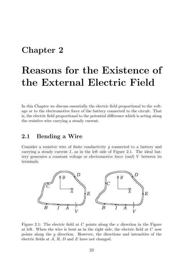
Consider a resistive wire of finite conductivity g connected to a battery andcarrying a steady current I, as in the left side of Figure 2.1. The ideal bat-tery generates a constant voltage or electromotive force (emf) V between itsterminals.

Figure 2.1: The electric field at C points along the x direction in the Figureat left. When the wire is bent as in the right side, the electric field at C nowpoints along the y direction. However, the directions and intensities of theelectric fields at A, B, D and E have not changed.

23

The current density ~J is given by ~J = (I/A)u, where A is the area of thecross section of the wire and the unit vector u points along the direction of thecurrent at every point in the interior of the wire. Ohm’s law in differential formstates that ~J = g ~E, where ~E is the electric field driving the current. By theprevious relation we see that ~E will also point along the direction of the wire ateach point.

Where are the charges which generate the electric field at each point alongthe wire located? It might be thought that this electric field is due to the battery(or to the charges located on the battery), but this is not the complete answer.To see that the battery does not generate the electric field at all points alongthe wire, we can consider Figure 2.1. We know that the electric field drivingthe constant current will in general follow the shape of the wire. At a specificpoint C inside the wire the electric field in Figure 2.1 (left circuit) points alongthe positive x direction. When we bend a portion of the wire, the electric fieldwill follow this bending. In the circuit at the right side of Figure 2.1 it can beseen that at the same point C the electric field now points toward the positivey direction.

If something changes inside the battery when we bend the wire, the electricfield at points closer to the battery would also change. However, the electricfield changes its path or direction only in the portion which was bent and inthe regions close to it, maintaining the previous values and directions in theother points (like the points A, B, D or E in Figure 2.1). As the electric fieldinside the wire has changed only in the bent portion, something local musthave created this change in the direction of the electric field. The shape ofthe wire has obviously changed. But as the shape or spatial configuration doesnot create an electric field, the reason must be sought elsewhere. What createselectric fields or the electric forces exerted upon the conduction electrons mustbe other charges, called here source charges. So there should exist a change inthe location of the source charges when we compare the configurations of theleft and right sides of Figure 2.1. And this change in the location of the sourcecharges should happen mainly around the bent portion of the wire, but not atthe battery. We then arrive at Weber’s and Kirchhoff’s idea that the electricfield inside a wire carrying a constant current is due to free charges spread alongthe surface of the wire [32, 24, 25, 26]. Kirchhoff’s three papers have Englishtranslations [27, 28, 29]. In the Appendices we discuss these works in moredetail. The role of the battery is to maintain this distribution of free chargesalong the surface of the wire (constant in time for steady currents, but variablealong the length of the wire). There will be a continuous gradient of density ofsurface charges along the length of the wire, more positive toward the positiveterminal of the battery, decreasing in magnitude until it reaches a zero value atan intermediary point, and increasingly negative toward the negative terminal,Figure 2.2.

If there were no battery, the charge density would be zero at all points alongthe surface of the wire. It is the distribution of these surface charges in spacewhich creates the electric field inside the wire driving the current. When webend a portion of the wire, the free charges redistribute themselves in space

24

Figure 2.2: Qualitative distribution of charges along the surface of a resistivewire carrying a steady current in two different configurations.

along the surface of the wire, creating the electric field which will follow thenew trajectory of the wire. This can be seen qualitatively in the right circuitof Figure 2.2. Supposing the wire to be globally neutral, the integration of thesurface charges σ along the whole surface of the wire must always go to zero,although σ is not zero at all points along the surface.

A qualitative representation of the surface charges in a resistive ring carryinga steady current I when connected to a battery generating a voltage V betweenits terminals is shown on the left side of Figure 2.3. A qualitative representationof the internal and external electric fields due to these surface charges is shownon the right side of Figure 2.3.

Figure 2.3: Qualitative representation of the surface charges (left) and of theinternal and external electric field (right) of a resistive ring carrying a steadycurrent.

A qualitative discussion of this redistribution of surface charges when a wireis bent was given by Parker [164], and by Chabay and Sherwood [165, 166].An order of magnitude calculation of the charges necessary to bend the electric

25

current I around a corner has been given by Rosser [167].

However, most authors are not aware of these surface charges and the relatedelectric field outside the wire, as we can see from the quotations presented above.Fortunately this subject has been revisited by other authors in some importantworks discussed in this book.

2.2 Continuity of the Tangential Component of

the Electric Field

A second reason for the existence of an electric field outside resistive conductorscarrying steady currents is related to the boundary conditions for the electricfield ~E. As is well known, at an interface between two media 1 and 2 (withn being the unit vector normal to the interface at every point) we have that

the tangential component of ~E is continuous, Et1 = Et2 or n× ( ~E2 − ~E1) = 0.On the other hand, the normal component may be discontinuous according ton · (ε2 ~E2− ε1 ~E1) = σ, where εj is the dielectric constant of the medium j and σis the density of surface charges at the interface. By Ohm’s law there must be alongitudinal component of ~E inside a resistive wire, even at its surface. As thiscomponent is continuous at an interface, it must also exist in vacuum or in theair outside the conductor, not only close by, but also at measurable distancesfrom the wire.

Many textbooks only consider an electric field outside the current-carryingwire when discussing these boundary conditions. The flux of energy in theelectromagnetic field is represented in classical electromagnetism by Poynting’svector ~S = ~E × ~B/µ0, where ~B is the magnetic field and µ0 = 4π × 10−7

H/m is the magnetic permeability of the vacuum. The authors who deal withthe electric field outside wires by considering the boundary conditions normallypresent Poynting’s vector pointing radially inwards toward the wire [168, pp.180-181] [33, p. 27-8]. This goes back to Poynting himself in 1885 [169, 170].Here is what Poynting wrote in this paper: “In the particular case of a steadycurrent in a wire where the electrical level surfaces cut the wire perpendicularlyto the axis, it appears that the energy dissipated in the wire as heat comes infrom the surrounding medium, entering perpendicularly to the surface.” (...)“In the neighbourhood of a wire containing a current, the electric tubes may ingeneral be taken as parallel to the wire while the magnetic tubes encircle it.”In the first paragraph of the section A straight wire carrying a steady currenthe wrote: “Let AB represent a wire in which is a steady current from A to B.The direction of the electric induction in the surrounding field near the wire, ifthe field be homogeneous, is parallel to AB.”

A typical representation found in the textbooks of the fields ~E, ~B and ~S inthe vicinity of a current carrying cylindrical wire is that of Figure 2.4.

There are two points to make here. In the first place, these drawings andstatements suggest that this electric field should exist only close to the wire,while as a matter of fact it exists at all points in space. In the second place,

26

Figure 2.4: Typical representation of the Poynting vector ~S = ~E× ~B/µ0 outsidea resistive wire carrying a steady current.

they indicate that these authors are not concerned about the surface chargesgenerating the field. It is only at a few locations that ~S will be orthogonal tothe wire just outside it, namely, the locations where the surface charge densitygoes to zero. These locations are an exception and not the rule. In most otherlocations the density of surface charges will be either positive (closer to thepositive terminal of the battery) or negative (closer to the negative terminal ofthe battery). The rule is that there will be a radial component which may belarger than the longitudinal one, pointing toward the wire or away from it. Oneof the effects of this radial component is that ~E and ~S will usually be inclinedjust outside the wire and not orthogonal to it.

These two misleading viewpoints are clearly represented by Feynman, Leightonand Sands’s statement in Section 27-5 (Examples of energy flow) of their book[33, p. 27-8], our emphasis in boldface: “As another example, we ask what hap-pens in a piece of resistance wire when it is carrying a current. Since the wirehas resistance, there is an electric field along it, driving the current. Becausethere is a potential drop along the wire, there is also an electric field justoutside the wire, parallel to the surface (see Fig. 27-5 [our Figure 2.4]).There is, in addition, a magnetic field which goes around the wire because of thecurrent. The E and B are at right angles; therefore there is a Poynting vectordirected radially inward, as shown in the figure. There is a flow of energy intothe wire all around. It is, of course, equal to the energy being lost in the wirein the form of heat. So our “crazy” theory says that the electrons are gettingtheir energy to generate heat because of the energy flowing into the wire fromthe field outside. Intuition would seem to tell us that the electrons get theirenergy from being pushed along the wire, so the energy should be flowing down(or up) along the wire. But the theory says that the electrons are really beingpushed by an electric field, which has come from some charges very far away,and that the electrons get their energy for generating heat from these fields.The energy somehow flows from the distant charges into a wide area of spaceand then inward to the wire.”

As we have seen, the electric field just outside the resistive wire is normally

27

not parallel to the wire. Moreover, the main contribution for the local electricfield at a specific point inside a wire is due to the charges along the surface ofthe wire around this point, contrary to their statement (who believed that it hascome “from some charges very far away”). Probably they were thinking here ofthe charges inside the battery.

28

Chapter 3

Experiments

In this Chapter we present experiments that prove the existence of the electricfield outside resistive wires carrying steady currents. Many experiments alongthese lines were probably performed in the second half of the XIXth centuryand in the early part of the XXth century, but they have been forgotten andare not quoted nowadays. Here we present only those which have come to ourattention.

We separate these experiments into three classes. The first one is related tothe zeroth order electric field (due to electrostatic induction), which exists evenwhen there is no current along the wire. The second class is related directly tothe battery and to the current along the wire, being proportional to the emf ofthe battery or to the potential difference acting along the conductor. The thirdclass is related to the second order electric field, proportional to v2

d/c2, where

vd is the drifting velocity of the conduction electrons and c is light velocity invacuum.

3.1 Zeroth Order Electric Field

We are not aware of any specific experiments designed to measure the forcebetween a point charge and a nearby conductor. We are here considering aconductor which is initially neutral and has no currents flowing through it, untilwe bring a charge close to it and let both of them at rest relative to one another.After the electrostatic equilibrium is reached, the electrical polarization of theconductor will cause a net force between the conductor and the external charge.This zeroth order force will depend upon the shape of the conductor, upon itsdistance to the external charge, and upon the value of this charge. We canalso express this by saying that a zeroth order electric field will be createddepending upon the external test charge, upon its distance to the conductorand upon the shape of the conductor. Many quantitative experiments alongthese lines were probably performed in the XIXth century. As we are not awareof them, we will not quote any specific experiment here. But we believe these

29

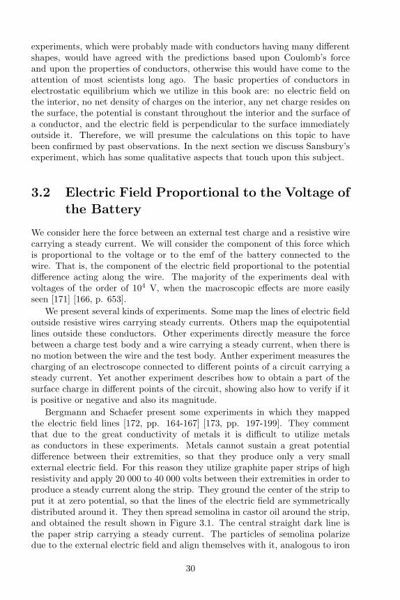
experiments, which were probably made with conductors having many differentshapes, would have agreed with the predictions based upon Coulomb’s forceand upon the properties of conductors, otherwise this would have come to theattention of most scientists long ago. The basic properties of conductors inelectrostatic equilibrium which we utilize in this book are: no electric field onthe interior, no net density of charges on the interior, any net charge resides onthe surface, the potential is constant throughout the interior and the surface ofa conductor, and the electric field is perpendicular to the surface immediatelyoutside it. Therefore, we will presume the calculations on this topic to havebeen confirmed by past observations. In the next section we discuss Sansbury’sexperiment, which has some qualitative aspects that touch upon this subject.

3.2 Electric Field Proportional to the Voltage of

the Battery

We consider here the force between an external test charge and a resistive wirecarrying a steady current. We will consider the component of this force whichis proportional to the voltage or to the emf of the battery connected to thewire. That is, the component of the electric field proportional to the potentialdifference acting along the wire. The majority of the experiments deal withvoltages of the order of 104 V, when the macroscopic effects are more easilyseen [171] [166, p. 653].

We present several kinds of experiments. Some map the lines of electric fieldoutside resistive wires carrying steady currents. Others map the equipotentiallines outside these conductors. Other experiments directly measure the forcebetween a charge test body and a wire carrying a steady current, when there isno motion between the wire and the test body. Anther experiment measures thecharging of an electroscope connected to different points of a circuit carrying asteady current. Yet another experiment describes how to obtain a part of thesurface charge in different points of the circuit, showing also how to verify if itis positive or negative and also its magnitude.

Bergmann and Schaefer present some experiments in which they mappedthe electric field lines [172, pp. 164-167] [173, pp. 197-199]. They commentthat due to the great conductivity of metals it is difficult to utilize metalsas conductors in these experiments. Metals cannot sustain a great potentialdifference between their extremities, so that they produce only a very smallexternal electric field. For this reason they utilize graphite paper strips of highresistivity and apply 20 000 to 40 000 volts between their extremities in order toproduce a steady current along the strip. They ground the center of the strip toput it at zero potential, so that the lines of the electric field are symmetricallydistributed around it. They then spread semolina in castor oil around the strip,and obtained the result shown in Figure 3.1. The central straight dark line isthe paper strip carrying a steady current. The particles of semolina polarizedue to the external electric field and align themselves with it, analogous to iron

30

filings mapping a magnetic field.

Figure 3.1: Experimental mapping of the external electric field of a straightconductor carrying a steady current.

It should be observed that along the external surface of the conductor thereis a longitudinal component of the electric field. This aspect differentiates itfrom the electric field outside conductors held at a constant potential (in whichcase the external electric field in steady state is normal to the conductor atevery point of its surface), as has been pointed out by Bergmann and Schaefer.

By bending the conductor in a U-form they were able to show the lines ofelectric field outside a transmission line or twin-lead, Figure 3.2. On the leftside the electric field lines are built into the plane of the conductors, while onthe right hand side they are built into a plane orthogonal to the conductors.

Figure 3.2: Experimental mapping of the external electric field of a transmissionline.

Bergmann and Schaefer also discuss the redistribution of charges along thesurface of an open circuit connected to a battery when the circuit is closed.Another clear discussion of this situation can be found in the recent book byChabay and Sherwood [165, Chapter 6].

Experiments similar to those of Bergmann and Schaefer have been performedby Jefimenko [174] [175, pp. 295-312 and 508-511] [176, plates 6 to 9 and pp.299-319 and 508-511]. He utilized a transparent conducting ink to make a two-

31

dimensional printed circuit on glass plates of 10 inches × 12 inches. In theFigures, 3.3 to 3.7 the gray sections represent the current-carrying conductingstrips. The power supply was capable of producing about 104 V. He utilizeda Du Mont high-voltage power supply type 263-A but mentioned that a smallvan de Graaff generator might also be employed. After the power supply wasturned on, he spread some fine grass seeds (Redtop type) over the plate andconducting system. The seeds lined up in the direction of the electric field overand outside the conductors.

Figure 3.3 depicts Jefimenko’s experiment for a straight current-carryingconductor.

Figure 3.3: Straight current-carrying conductor.

Figure 3.4 depicts his experiment for square-shaped (left) and circular (right)conducting rings.

Figure 3.4: Square-shaped (left) and circular (right) conducting rings.

Figure 3.5 depicts his experiment for shorted symmetric (left) and asymmet-ric (right) transmission lines.

Figure 3.6 depicts his experiment for current-carrying wedges with the twohalves connected in parallel (left) and in series (right).

And Figure 3.7 depicts his experiments involving current-carrying rings onthe left with two-pole (top) and four-pole (bottom) connections. On the rightwe have current-carrying discs with two-pole (top) and four-pole (bottom) con-nections.

32

Figure 3.5: Shorted symmetric (left) and asymmetric (right) transmission lines.

Figure 3.6: Current-carrying wedges with the two halves connected in parallel(left) and in series (right).

Figure 3.7: On the left are current-carrying rings with two-pole (top) and four-pole (bottom) connections. On the right are current-carrying discs with two-pole(top) and four-pole (bottom) connections.

33

In a private communication to one of the authors (AKTA), Jefimenko men-tioned that he never measured the current in the grass seed experiments. How-ever, he believed that they were of the order of a few microamperes. He men-tioned that the patterns of the current-carrying conductors were about 16 or 20centimeters long.

The experiments of Bergmann, Schaefer and Jefimenko complement one an-other. After obtaining theoretical formulas for the equipotentials and for theelectric field lines, we will compare them with some of these experimental results.

In another type of experiment, Jefimenko, Barnett and Kelly obtained theequipotential lines directly inside and outside conductors with steady currentsutilizing an electronic electrometer [177] [176, p. 301]. A radioactive alpha-source was utilized to ionize the air, in order to make it a conductor of electricity,at the point where the field was to be measured. The alpha-source acquiredthe same potential as the field at that point. The potential was measured(in relation to a reference point chosen at zero potential) with an electronicelectrometer connected to the alpha-source. They utilized a hollow rectangularchamber with electrodes for end walls and semi-conducting side walls carryinguniform current. Graphite paper strips were used for the side walls, as in theexperiments by Bergmann and Schaefer, and aluminum foil served as electrodeswith 80 V applied. The equipotentials were mapped experimentally.

Figure 3.8 depicts the configuration of the problem.

Figure 3.8: Configuration of the system.

Figure 3.9 depicts the equipotential lines measured in one of the experiments.

Figure 3.9: Measured equipotentials.

In another experiment, undeveloped photographic film was used in place of

34

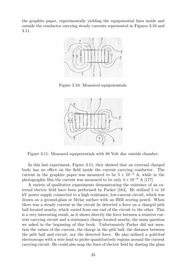
the graphite paper, experimentally yielding the equipotential lines inside andoutside the conductor carrying steady currents represented in Figures 3.10 and3.11.

Figure 3.10: Measured equipotentials.

Figure 3.11: Measured equipotentials with 80 Volt disc outside chamber.

In this last experiment, Figure 3.11, they showed that an external chargedbody has no effect on the field inside the current carrying conductor. Thecurrent in the graphite paper was measured to be 5 × 10−2 A, while in thephotographic film the current was measured to be only 4 × 10−6 A [177].

A variety of qualitative experiments demonstrating the existence of an ex-ternal electric field have been performed by Parker [164]. He utilized 5 to 10kV power supply connected to a high resistance, low-current circuit, which wasdrawn on a ground-glass or Mylar surface with an IBM scoring pencil. Whenthere was a steady current in the circuit he detected a force on a charged pithball located nearby, which varied from one end of the circuit to the other. Thisis a very interesting result, as it shows directly the force between a resistive cur-rent carrying circuit and a stationary charge located nearby, the main questionwe asked in the beginning of this book. Unfortunately Parker did not men-tion the values of the current, the charge in the pith ball, the distance betweenthe pith ball and circuit, nor the detected force. He also utilized a gold-leafelectroscope with a wire lead to probe quantitatively regions around the currentcarrying circuit. He could also map the lines of electric field by dusting the glass

35

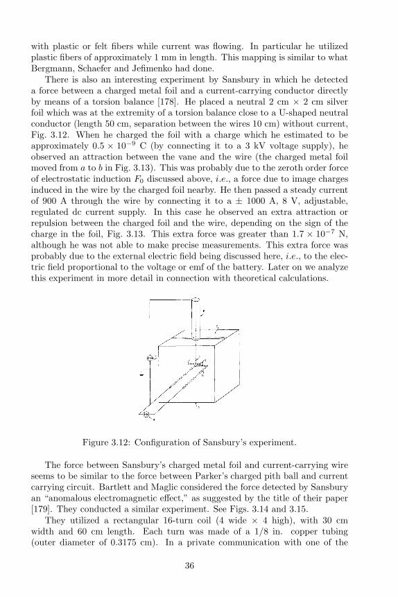
with plastic or felt fibers while current was flowing. In particular he utilizedplastic fibers of approximately 1 mm in length. This mapping is similar to whatBergmann, Schaefer and Jefimenko had done.

There is also an interesting experiment by Sansbury in which he detecteda force between a charged metal foil and a current-carrying conductor directlyby means of a torsion balance [178]. He placed a neutral 2 cm × 2 cm silverfoil which was at the extremity of a torsion balance close to a U-shaped neutralconductor (length 50 cm, separation between the wires 10 cm) without current,Fig. 3.12. When he charged the foil with a charge which he estimated to beapproximately 0.5 × 10−9 C (by connecting it to a 3 kV voltage supply), heobserved an attraction between the vane and the wire (the charged metal foilmoved from a to b in Fig. 3.13). This was probably due to the zeroth order forceof electrostatic induction F0 discussed above, i.e., a force due to image chargesinduced in the wire by the charged foil nearby. He then passed a steady currentof 900 A through the wire by connecting it to a ± 1000 A, 8 V, adjustable,regulated dc current supply. In this case he observed an extra attraction orrepulsion between the charged foil and the wire, depending on the sign of thecharge in the foil, Fig. 3.13. This extra force was greater than 1.7 × 10−7 N,although he was not able to make precise measurements. This extra force wasprobably due to the external electric field being discussed here, i.e., to the elec-tric field proportional to the voltage or emf of the battery. Later on we analyzethis experiment in more detail in connection with theoretical calculations.

Figure 3.12: Configuration of Sansbury’s experiment.

The force between Sansbury’s charged metal foil and current-carrying wireseems to be similar to the force between Parker’s charged pith ball and currentcarrying circuit. Bartlett and Maglic considered the force detected by Sansburyan “anomalous electromagnetic effect,” as suggested by the title of their paper[179]. They conducted a similar experiment. See Figs. 3.14 and 3.15.

They utilized a rectangular 16-turn coil (4 wide × 4 high), with 30 cmwidth and 60 cm length. Each turn was made of a 1/8 in. copper tubing(outer diameter of 0.3175 cm). In a private communication with one of the

36

Figure 3.13: In the beginning there is no current in the conductor and theuncharged silver foil remains at a. When the silver foil is charged, it movesfrom a to b. Then a steady current I is passed through the conductor. In thiscase there appears an extra force of attraction or repulsion between the chargedfoil and the U -shaped conductor.

authors (JAH) Bartlett reported that the conductor was water-cooled, withwater flowing through the hole in the center of the tubing. Approximately 50%of the cross-sectional area of the tubing was copper, and 50% was water. Acurrent source connected to the coil maintained a steady current of 50 A in eachturn. They detected a force upon the charged metal foil with an area of 2.54cm × 2.54 cm placed at a distance of 3.5 cm from the coil carrying a steadycurrent. This was similar to the effect detected by Sansbury.

Figure 3.14: Experiment performed by Bartlett and Maglic.

But when the upper half of the current carrying circuit and the test chargewere shielded with an aluminum can, the effect disappeared. Their conclusionwas that they could not find this “anomalous” interaction, implying that it did

37

Figure 3.15: Top view of Bartlett and Maglic’s experiment.

not exist.However, they seem to have been unaware of one important point in connec-

tion with Faraday cages. They are usually utilized to shield the system underconsideration from external influences. But they affect the net force on each in-ternal test charge. For instance, if we have two charges q1 and q2 separated by adistance d, the coulombian force between them has a magnitude of q1q2/4πε0d

2

and is directed along the line joining them, Figure 3.16.

Figure 3.16: Electrostatic force between two charges far from other charges andconductors.

When we surround both of them with a metallic shell, they will induce adistribution of charges along the surface of the shell. As a result of these inducedcharges, the shell will exert forces on q1 and on q2, resulting in general in a netforce on each one of them different from the previous value of q1q2/4πε0d

2.With a spherical shell the force upon the internal test charges exerted by theinduced charges along the wall can be easily calculated by the method of images.Each charge qj located at a distance aj from the center of the shell of radiusr0 > aj , with j = 1 or 2, will induce charges equivalent to an image chargeqij = −qjr0/aj at a distance aij = r20/aj > r0 from the center of the shell,located along the straight line connecting the center of the shell and qj . The

net force on q1, for instance, will be given by ~F21 + ~Fi1,1 + ~Fi2,1 instead of simply~F21. Here ~Fm,n is the force exerted by the (image) charge m on the charge n. If

38

the straight line connecting the two charges q1 and q2 does not pass through thecenter of the shell, the net force on each one of them will change its magnitudeand also its direction in comparison with the previous value without the shell,Figure 3.17.

Figure 3.17: Electrostatic forces on q1 due to q2, to the image charge qi1 and tothe image charge qi2.

If there are N internal charges, the net force on q1 will be given by thesum of the forces due to the other N − 1 charges on q1, plus the N forces ofthe image charges on q1. If the Faraday cage is not spherical, it will be verydifficult to calculate the new force on the test charges. In Bartlett and Maglic’scase the Faraday cage was cylindrical with metallic lateral sides and dielectricextremities. This makes it very difficult to estimate the effect of the shieldupon the internal charged foil. Moreover, we have not just the two chargesq1 and q2 as discussed before, but the charged foil and a quantity of chargesdistributed along the surface of the resistive current-carrying wire. As the wire ismade of a conducting material, the induced charges upon the Faraday cage willchange the distribution of charges spread along the surface of the wire (comparedwith the distribution of surface charges without the Faraday cage), such thateven this new distribution is not yet known until they can be calculated withLaplace’s equation and the appropriate boundary conditions. This enormouslycomplicates the theoretical analysis of the expected net force (exerted upon thetest charge when the current-carrying wire and the test charge are shielded).For this reason it seems preferable to perform this kind of experiment withoutthe metallic shield.

The result obtained by Bartlett and Maglic is described as follows [179]:“Averaging the results of the runs with and without the shield we find a signalof 0.3 ± 0.3 mrad. (...) We multiply our measured rotation of 0.3 ± 0.3 mrad bythe sensitivity of the fiber (9.1×10−5 N/m) to obtain a force of (0.27±0.27)10−7

N.” The impression we get from reading the paper is that the force measuredwithout the shield was 0.27 × 10−7 N, one order of magnitude smaller thanthat observed by Sansbury. On the other hand, we infer that with the shieldBartlett and Maglic measured no force (hence the ± sign given in the previousquotation). Our opinion is that the shield changes the distribution of charges

39

on the metallic shell. This changes the net force on each of the internal charges,as we showed earlier. Therefore, it is very difficult to compare the two cases(with and without shielding). The ideal situation would be to perform this kindof experiment without any shield. Unfortunately, this was not the procedureadopted by Bartlett and Maglic.

Further discussions of Sansbury’s experiment with different approaches canbe found in works by several authors [1, 4, 5, 82, 83, 180, 181, 182, 183].

Another kind of experiment was performed by Moreau, Ryan, Beuzenbergand Syme [184]. (See Figure 3.18.)

Figure 3.18: Electroscope touching different points of a high voltage resistivecircuit carrying a steady current.

They connected a 0- to 5-kV current-limited dc power supply to a seriescircuit consisting of two resistances of 75 MΩ. The conductors were bare alu-minum bars and the resistances were strips of foam plastic impregnated withAqua Dac. The conductors and resistances had rectangular cross-sections of 12mm × 9 mm. Each one of the resistances was 50 cm in length. The conductingbar between them was 30 cm in length. The main goal of the experiment wasto demonstrate directly that when a steady current flows along a circuit, thereis a gradient of surface charges along the conductors and along the resistances,in such a way that this gradient of surface charge density produces an electricfield along the direction of the current. To indicate the charge density at sev-eral points of the circuit, they connected these points to a high voltage probe.This probe was connected to a gold-leaf electroscope. Something similar to thiswas done by Parker [164]. The electroscope was placed inside a nonconductingpolystyrene case. When the power supply was turned up to 2 kV a microamme-ter in the circuit measured a current of about 13 µA. One side of the circuit wasgrounded. At this point the electroscope showed no deflection, indicating zerocharge density. As the probe moved away from this point along the resistancestrip, the electroscope deflected gradually with distance traveled along the re-sistance, reaching a deflection of about 55o at its end. The deflection remained

40

constant as the probe was moved along the middle conductor, indicating thatthe charge density was essentially constant (or that it varied very little) alongit. The deflection increased again along the second resistance, reaching a finaldeflection of about 70o at the extremity. This indicated that the charge den-sity was relatively high on the upstream side of the resistors, decreasing alongthem in the direction of the current. This produced an electric field forcing theconduction charges through the resistances.

Another very didactic experience was performed by Uri Ganiel and collabo-rators of the Science Education Group at the Weizmann Institute in Israel. Thisexperiment has been cited and reproduced by Chabay and Sherwood [171, 185][166, Section 18.10, pp x and 652-654]. (See Figure 3.19.)

Figure 3.19: Four identical high resistance resistors are connected in series ina closed circuit carrying a steady current. This Figure shows the qualitativedistribution of surface charges. The thin metallized mylar strip is attracted bythe bare (uninsulated) wires, touches them and is then repelled by them. Bytesting the charge gained by the metallized strip it is possible to determine thesign of the surface charges at each point along the circuit.

A closed circuit is formed with four identical high resistance resistors con-nected in series, each with 80 MΩ. They are connected to two high voltagepower supplies, of 5 kV each. There is a grounded conductor between thesetwo power supplies. One of the power supplies yields + 5 kV at one extremityof the first resistor, while the other yields - 5 kV at the opposite extremity ofthe fourth resistor (relative to the ground). In other words, these two powersupplies are connected in series. There are bare (uninsulated) wires betweenthe resistors in order to allow the collection of their surface charges by an ap-propriate probe. This is performed utilizing a flexible, thin metallized mylarstrip. When the strip is brought close to the bare wire at the left side of thecircuit, near location A, it is observed to be attracted to the wire. It touchesthe wire and is then repelled by it. It is initially attracted due to polarizationof the aluminized plastic strip created by the surface charge on the wire. Whenit touches the wire, it jumps away, since it is charged by contact with the barewire and repelled by the surface charge at that location. When the strip istested it is found to be negatively charged. It is then discharged, and the same

41

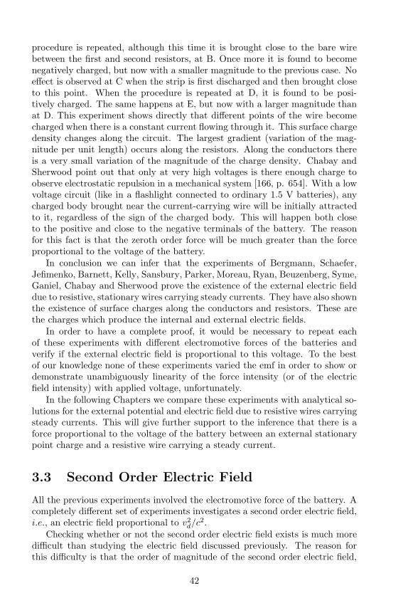
procedure is repeated, although this time it is brought close to the bare wirebetween the first and second resistors, at B. Once more it is found to becomenegatively charged, but now with a smaller magnitude to the previous case. Noeffect is observed at C when the strip is first discharged and then brought closeto this point. When the procedure is repeated at D, it is found to be posi-tively charged. The same happens at E, but now with a larger magnitude thanat D. This experiment shows directly that different points of the wire becomecharged when there is a constant current flowing through it. This surface chargedensity changes along the circuit. The largest gradient (variation of the mag-nitude per unit length) occurs along the resistors. Along the conductors thereis a very small variation of the magnitude of the charge density. Chabay andSherwood point out that only at very high voltages is there enough charge toobserve electrostatic repulsion in a mechanical system [166, p. 654]. With a lowvoltage circuit (like in a flashlight connected to ordinary 1.5 V batteries), anycharged body brought near the current-carrying wire will be initially attractedto it, regardless of the sign of the charged body. This will happen both closeto the positive and close to the negative terminals of the battery. The reasonfor this fact is that the zeroth order force will be much greater than the forceproportional to the voltage of the battery.

In conclusion we can infer that the experiments of Bergmann, Schaefer,Jefimenko, Barnett, Kelly, Sansbury, Parker, Moreau, Ryan, Beuzenberg, Syme,Ganiel, Chabay and Sherwood prove the existence of the external electric fielddue to resistive, stationary wires carrying steady currents. They have also shownthe existence of surface charges along the conductors and resistors. These arethe charges which produce the internal and external electric fields.

In order to have a complete proof, it would be necessary to repeat eachof these experiments with different electromotive forces of the batteries andverify if the external electric field is proportional to this voltage. To the bestof our knowledge none of these experiments varied the emf in order to show ordemonstrate unambiguously linearity of the force intensity (or of the electricfield intensity) with applied voltage, unfortunately.

In the following Chapters we compare these experiments with analytical so-lutions for the external potential and electric field due to resistive wires carryingsteady currents. This will give further support to the inference that there is aforce proportional to the voltage of the battery between an external stationarypoint charge and a resistive wire carrying a steady current.

3.3 Second Order Electric Field

All the previous experiments involved the electromotive force of the battery. Acompletely different set of experiments investigates a second order electric field,i.e., an electric field proportional to v2

d/c2.

Checking whether or not the second order electric field exists is much moredifficult than studying the electric field discussed previously. The reason forthis difficulty is that the order of magnitude of the second order electric field,

42

E2, is normally much smaller than the electric field associated with the electro-motive force of the battery, E1, and also much smaller than the zeroth orderelectric field, E0. However, if the wire is a superconductor and a steady currentis flowing through (with no battery connected to the wire), the external electricfield E1 should go to zero. If we take into account (or neglect) the force dueto electrostatic induction (related with image charges) as well, there remains inthis case only the second order electric field. This was the approach utilized byEdwards, Kenyon and Lemon in their experiments [14, 15], which are the bestknown to us to analyze this effect. They utilized type II superconductor (48%niobium and 52% titanium) cores of 2.5 mil radius with currents of the order of16 A. They found an electric field proportional to I2, independent of the direc-tion of the current, pointing toward the wire and with an order of magnitudecompatible with that predicted by Weber’s law. What they actually measuredutilizing an electrometer was a potential difference between the circuit and anelectrostatic shield around the circuit. They measured potential differences withan order of magnitude of 10 mV.

Bartlett and Ward made a number of different experiments to detect thissecond order electric field (which they interpreted as due to a possible variationof the electron’s charge with its velocity), but failed to find it [186]. Theyutilized normal resistive conductors, but in their analysis they did not mentionthe electric field proportional to the voltage of the battery discussed above.

In another experiment, Kenyon and Edwards placed a beam-power radiotube within a Faraday cage [187]. They tried to measure the potential differencebetween the system and the Faraday cage. They could not find any effectwith the order of magnitude of the earlier experiment of Edwards, Kenyon andLemon.

In any event attention must be called here to the Faraday cage aroundthe system in these experiments, and also in most of those quoted by Bartlettand Ward. As we mentioned previously, the charges induced in the walls of aFaraday cage due to internal charges will exert a net force on any internal testcharge. If there are two or more internal charges, the net force in each will bedifferent in two cases: (A) without the Faraday cage (force due only to the otherinternal charges), and (B) with Faraday cage (force due to the other internalcharges and to all induced charges in the walls of the cage). This enormouslycomplicates the analysis of all these experiments, and it is difficult to reach asimple result. Beyond the complication of the Faraday cage, there is also theelectric field proportional to the voltage of the battery which must be taken intoaccount before discussing the second order electric field. And this was not doneby any of these authors when dealing with resistive conductors. The secondorder electric field is usually much smaller than the electric field proportional tothe voltage of the battery, as we will show later on. For this reason the electricfield proportional to the voltage of the battery must be included in the analysisbecause it can mask the effect which is being sought.

More research is necessary before a final conclusion can be drawn on thissecond order electric field. A great number of experimental and theoreticalworks in connection with this subject have been published in the last 25 years

43

[188, 189, 190, 191, 82, 192, 181, 193, 83, 4, 5, 182, 194, 195, 196, 197, 23, 6, 7,198].

44

Chapter 4

Force Due to Electrostatic

Induction

4.1 Introduction

The main subject of this book is the force between a stationary wire carrying asteady current and an external charge at rest relative to the wire. In particular,we are interested in the component of this force which is proportional to thevoltage or emf of the battery, or to the potential difference acting along thewire.

Before analyzing these cases we consider the force between a point chargeand a conductor which has no current flowing through it. We suppose air orvacuum outside the conductor (and also inside hollow ones). We also consideronly the equilibrium situation when the point charge and the conductor areat rest relative to one another and also at rest relative to an inertial frame ofreference. It is also assumed that there are no other charges or conductors inthe vicinity of the system, beyond the ones being considered here. The mainmaterial of this Chapter was discussed in 2005 [199].

4.1.1 Point Charge and Infinite Plane

The simplest configuration is that of a point charge q at a distance d froman infinite conducting plane with zero net charge. Let us suppose that theconducting plane is along the plane z = 0, while the charge q is located at(x, y, z) = (0, 0, z). The method of images yields in this case an attractive forceacting upon q given by

~F0 = ∓ q2

16πε0

z

z2. (4.1)

Here the top sign is valid for z > 0, while the bottom sign is valid for z < 0.

45

Expressing this force as ~F0 = q ~E0 yields a zeroth order electric field givenby

~E0 = ∓ q

16πε0

z

z2. (4.2)

Even adding a finite charge Q uniformly spread along the infinite plane doesnot change these two results. That is, ~F0 and ~E0 are independent of Q.

This force is always attractive and diverges to infinity when d→ 0.

4.1.2 Point Charge and Spherical Shell

Another simple case to consider is that of a point charge and a conductingspherical shell at rest relative to one another. We consider a spherical shell ofradius R centered upon the origin 0 of a coordinate system. There is a netcharge Q on the conducting spherical shell, insulated from the earth. The testcharge q is located at ~r = rr relative to 0. The solution of this problem canalso be obtained by the method of images and is found in most textbooks onelectromagnetism. When r > R the force upon q is given by

~F0 =q

4πε0

[

Q− qR3(2r2 −R2)

r(r2 −R2)2

]

~r

r3. (4.3)

When r < R the force is independent of Q and is given by

~F0 =q2

4πε0

R~r

(R2 − r2)2. (4.4)

These forces diverge to infinity when r → R. When q is inside the shell, italways suffers an electrostatic force toward the closest wall. When q is outsidethe shell, the force will be attractive not only when qQ < 0, but also whenqQ > 0, provided q is at a very close distance to the shell. A detailed discussionof this fact can be found, for instance, in Maxwell’s work [200, Chapter VII:Theory of electrical images, pp. 80-88], in a paper by Melehy [201] and inJackson’s book [11, Section 2.3].

The zeroth order electric field in these cases is given by (with ~F0 = q ~E0):

~E0 =1

4πε0

[

Q− qR3(2r2 −R2)

r(r2 −R2)2

]

~r

r3, if r > R . (4.5)

~E0 =q

4πε0

R~r

(R2 − r2)2, if r < R . (4.6)

4.2 Point Charge and Cylindrical Shell

After considering these two simple cases we analyze the main subject of thischapter. The goal is to calculate the electrostatic force between an infiniteconducting cylinder of radius a held at zero potential and an external point

46

charge q. To the best of our knowledge this has never been done before. Tothis end we consider the Green function method [13, Chaps. 1 to 3]. We beginreviewing a known solution of the potential inside a grounded, closed, hollowand finite cylindrical shell with an internal point charge [13, p. 143]. We analyzethe limit of an infinite cylinder and explore the force exerted on the point charge.We then perform a similar analysis for the case of an external point charge. Weconsider in detail the particular situation of a thin wire, i.e., with the pointcharge many radii away from the axis of the cylinder. These calculations werepublished in 2005 [199].

4.3 Finite Conducting Cylindrical Shell with In-

ternal Point Charge: Solution of Poisson’s

Equation

Consider a finite conducting cylindrical shell of radius a and length ℓ ≫ a,with z being its axis of symmetry. (See Fig. 4.1.) With cylindrical coordinates(ρ, ϕ, z) the center of the shell is supposed to be at (ρ, z) = (0, ℓ/2). We alsoconsider a point charge q located at ~r ′ = (ρ′ < a,ϕ′, z′) inside the shell. We wishto calculate the electric potential of the system, the electric field, the surfacecharge distribution induced by q and the net force between the cylinder and q.

Figure 4.1: Finite conducting cylinder of length ℓ and radius a centered at(ρ, z) = (0, ℓ/2), with z being its axis of symmetry. There are conducting coversat z = 0 and at z = ℓ. There is a point charge q located at (ρ, ϕ, z) = (ρ′ <a,ϕ′, 0 < z′ < ℓ).

The electrostatic potential φ obeys Poisson’s equation:

∇2rφ = − ρ

ε0. (4.7)

By the standard Green function method, the solution of Poisson’s equationfor this case with Dirichlet boundary conditions (potential specified on a closedsurface) is given by:

47

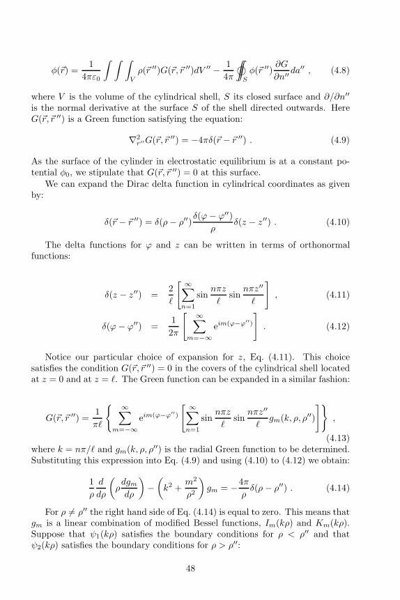
φ(~r) =1

4πε0

∫ ∫ ∫

V

ρ(~r ′′)G(~r, ~r ′′)dV ′′ − 1

4π©∫∫

S

φ(~r ′′)∂G

∂n′′ da′′ , (4.8)

where V is the volume of the cylindrical shell, S its closed surface and ∂/∂n′′

is the normal derivative at the surface S of the shell directed outwards. HereG(~r, ~r ′′) is a Green function satisfying the equation:

∇2r′′G(~r, ~r ′′) = −4πδ(~r − ~r ′′) . (4.9)

As the surface of the cylinder in electrostatic equilibrium is at a constant po-tential φ0, we stipulate that G(~r, ~r ′′) = 0 at this surface.

We can expand the Dirac delta function in cylindrical coordinates as givenby:

δ(~r − ~r ′′) = δ(ρ− ρ′′)δ(ϕ− ϕ′′)

ρδ(z − z′′) . (4.10)

The delta functions for ϕ and z can be written in terms of orthonormalfunctions:

δ(z − z′′) =2

ℓ

[ ∞∑

n=1

sinnπz

ℓsin

nπz′′

ℓ

]

, (4.11)

δ(ϕ− ϕ′′) =1

2π

[ ∞∑

m=−∞eim(ϕ−ϕ′′)

]

. (4.12)

Notice our particular choice of expansion for z, Eq. (4.11). This choicesatisfies the condition G(~r, ~r ′′) = 0 in the covers of the cylindrical shell locatedat z = 0 and at z = ℓ. The Green function can be expanded in a similar fashion:

G(~r, ~r ′′) =1

πℓ

∞∑

m=−∞eim(ϕ−ϕ′′)

[ ∞∑

n=1

sinnπz

ℓsin

nπz′′

ℓgm(k, ρ, ρ′′)

]

,

(4.13)where k = nπ/ℓ and gm(k, ρ, ρ′′) is the radial Green function to be determined.Substituting this expression into Eq. (4.9) and using (4.10) to (4.12) we obtain:

1

ρ

d

dρ

(

ρdgmdρ

)

−(

k2 +m2

ρ2

)

gm = −4π

ρδ(ρ− ρ′′) . (4.14)

For ρ 6= ρ′′ the right hand side of Eq. (4.14) is equal to zero. This means thatgm is a linear combination of modified Bessel functions, Im(kρ) and Km(kρ).Suppose that ψ1(kρ) satisfies the boundary conditions for ρ < ρ′′ and thatψ2(kρ) satisfies the boundary conditions for ρ > ρ′′:

48

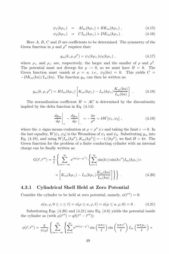
ψ1(kρ<) = AIm(kρ<) +BKm(kρ<) , (4.15)

ψ2(kρ>) = CIm(kρ>) +DKm(kρ>) . (4.16)

Here A, B, C and D are coefficients to be determined. The symmetry of theGreen function in ρ and ρ′′ requires that:

gm(k, ρ, ρ′′) = ψ1(kρ<)ψ2(kρ>) , (4.17)

where ρ> and ρ< are, respectively, the larger and the smaller of ρ and ρ′′.The potential must not diverge for ρ → 0, so we must have B = 0. TheGreen function must vanish at ρ = a, i.e., ψ2(ka) = 0. This yields C =−DKm(ka)/Im(ka). The function gm can then be written as:

gm(k, ρ, ρ′′) = HIm(kρ<)

[

Km(kρ>) − Im(kρ>)Km(ka)

Im(ka)

]

. (4.18)

The normalization coefficient H = AC is determined by the discontinuityimplied by the delta function in Eq. (4.14):

dgmdρ

∣

∣

∣

∣

∣

+

− dgmdρ

∣

∣

∣

∣

∣

−

= −4π

ρ′′= kW [ψ1, ψ2] , (4.19)

where the ± signs means evaluation at ρ = ρ′′± ǫ and taking the limit ǫ→ 0. Inthe last equality, W [ψ1, ψ2] is the Wronskian of ψ1 and ψ2. Substituting gm intoEq. (4.19), and using W [Im(kρ′′),Km(kρ′′)] = −1/(kρ′′), we find H = 4π. TheGreen function for the problem of a finite conducting cylinder with an internalcharge can be finally written as:

G(~r, ~r ′′) =4

ℓ

∞∑

m=−∞eim(ϕ−ϕ′′)

∞∑

n=1

sin(kz) sin(kz′′)Im(kρ<)×

×[

Km(kρ>) − Im(kρ>)Km(ka)

Im(ka)

]

. (4.20)

4.3.1 Cylindrical Shell Held at Zero Potential

Consider the cylinder to be held at zero potential, namely, φ(~r ′′) = 0:

φ(a, ϕ, 0 ≤ z ≤ ℓ) = φ(ρ ≤ a, ϕ, ℓ) = φ(ρ ≤ a, ϕ, 0) = 0 . (4.21)

Substituting Eqs. (4.20) and (4.21) into Eq. (4.8) yields the potential insidethe cylinder as (with ρ(~r ′′) = qδ(~r ′ − ~r ′′)):

φ(~r, ~r ′) =q

πε0ℓ

∞∑

m=−∞

∞∑

n=1

eim(ϕ−ϕ′) sin(nπz

ℓ

)

sin

(

nπz′

ℓ

)

Im

(nπρ<ℓ

)

×

49

×[

Km

(nπρ>ℓ

)

− Im

(nπρ>ℓ

) Km

(

nπaℓ

)

Im(

nπaℓ

)

]

. (4.22)

Here ρ> (ρ<) is the larger (smaller) of ρ and ρ′.

4.4 Infinite Conducting Cylindrical Shell with

Internal Point Charge

We now expand Jackson’s solution for the case of a cylindrical shell of infinitelength.

The solution for an infinite cylinder differs from the solution of the finitecylinder in that it essentially changes the expansion of the delta function inEq. (4.11). In the infinite cylinder there is no restriction on the choice of n (ork):

δ(z − z′′) =1

2π

∫ ∞

−∞eik(z−z

′′)dk =1

π

∫ ∞

0

cos[k(z − z′′)]dk . (4.23)

The Green function can be written as:

G(~r, ~r ′′) =2

π

∞∑

m=−∞eim(ϕ−ϕ′′)

∫ ∞

0

cos[k(z − z′′)]Im(kρ<)×

×[

Km(kρ>) − Im(kρ>)Km(ka)

Im(ka)

]

dk

. (4.24)

Note that we can pass from Eq. (4.11) to Eq. (4.23) by transforming theFourier series into the Fourier transform, that is, by letting ℓ → ∞, settingnπ/ℓ = k, dk = π/ℓ, z → z + ℓ/2, z′′ → z′′ + ℓ/2 and by replacing the infinitesum by the integral over k.

4.4.1 Cylindrical Shell Held at Zero Potential

Consider the cylinder to be held at zero potential, namely, φ(a, ϕ, z) = 0. Substi-tuting Eq. (4.24) into Eq. (4.8), the potential inside the cylinder can be writtenas (with ρ(~r ′′) = qδ(~r ′ − ~r ′′)):

φ(~r, ~r ′) =q

2π2ε0

∞∑

m=−∞eim(ϕ−ϕ′)

∫ ∞

0

cos[k(z − z′)]Im(kρ<)×

×[

Km(kρ>) − Im(kρ>)Km(ka)

Im(ka)

]

dk

. (4.25)

Once more ρ> (ρ<) is the larger (smaller) of ρ and ρ′.

50

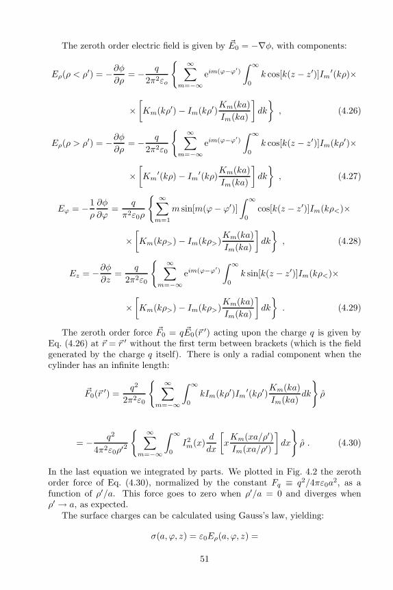
The zeroth order electric field is given by ~E0 = −∇φ, with components:

Eρ(ρ < ρ′) = −∂φ∂ρ

= − q

2π2εo

∞∑

m=−∞eim(ϕ−ϕ′)

∫ ∞

0

k cos[k(z − z′)]Im′(kρ)×

×[

Km(kρ′) − Im(kρ′)Km(ka)

Im(ka)

]

dk

, (4.26)

Eρ(ρ > ρ′) = −∂φ∂ρ

= − q

2π2ε0

∞∑

m=−∞eim(ϕ−ϕ′)

∫ ∞

0

k cos[k(z − z′)]Im(kρ′)×

×[

Km′(kρ) − Im

′(kρ)Km(ka)

Im(ka)

]

dk

, (4.27)

Eϕ = −1

ρ

∂φ

∂ϕ=

q

π2ε0ρ

∞∑

m=1

m sin[m(ϕ− ϕ′)]

∫ ∞

0

cos[k(z − z′)]Im(kρ<)×

×[

Km(kρ>) − Im(kρ>)Km(ka)

Im(ka)

]

dk

, (4.28)

Ez = −∂φ∂z

=q

2π2ε0

∞∑

m=−∞eim(ϕ−ϕ′)

∫ ∞

0

k sin[k(z − z′)]Im(kρ<)×

×[

Km(kρ>) − Im(kρ>)Km(ka)

Im(ka)

]

dk

. (4.29)

The zeroth order force ~F0 = q ~E0(~r′) acting upon the charge q is given by

Eq. (4.26) at ~r = ~r ′ without the first term between brackets (which is the fieldgenerated by the charge q itself). There is only a radial component when thecylinder has an infinite length:

~F0(~r′) =

q2

2π2ε0

∞∑

m=−∞

∫ ∞

0

kIm(kρ′)Im′(kρ′)

Km(ka)

Im(ka)dk

ρ

= − q2

4π2ε0ρ′2

∞∑

m=−∞

∫ ∞

0

I2m(x)

d

dx

[

xKm(xa/ρ′)

Im(xa/ρ′)

]

dx

ρ . (4.30)

In the last equation we integrated by parts. We plotted in Fig. 4.2 the zerothorder force of Eq. (4.30), normalized by the constant Fq ≡ q2/4πε0a

2, as afunction of ρ′/a. This force goes to zero when ρ′/a = 0 and diverges whenρ′ → a, as expected.

The surface charges can be calculated using Gauss’s law, yielding:

σ(a, ϕ, z) = ε0Eρ(a, ϕ, z) =

51

Figure 4.2: Zeroth order force F0 between an infinite grounded conducting cylin-der of radius a and a point charge q at a distance ρ′ < a from the z axis(which is also the axis of symmetry of the cylinder), normalized by the constantFq ≡ q2/4πε0a

2.

= − q

2π2a

[ ∞∑

m=−∞eim(ϕ−ϕ′)

∫ ∞

0

cos[k(z − z′)]Im(kρ′)

Im(ka)dk

]

. (4.31)

The charge per unit length λ(z) is given by:

λ(a, z) =

∫ 2π

0

σ(a, ϕ, z)a dϕ = − q

π

∫ ∞

0

cos[k(z − z′)]I0(kρ

′)

I0(ka)dk . (4.32)

The total charge induced in the cylinder, supposing z′ = 0, can be obtainedintegrating Eq. (4.32) from z = −∞ to ∞. Utilizing:

δ(k) =1

2π

∫ ∞

−∞cos(kz)dz =

1

π

∫ ∞

0

cos(kz)dz , (4.33)

this yields:

Q =

∫ ∞

−∞λ(a, z)dz = −q . (4.34)

4.5 Infinite Conducting Cylindrical Shell with

External Point Charge

We can now consider a new case, i.e., a conducting cylinder with an externalpoint charge. Suppose that the point charge q is located at ~r ′ = (ρ′, ϕ′, z′),with ρ′ > a. Green function can be written analogously in this case as:

G(~r, ~r ′′) =1

2π2

[ ∞∑

m=−∞eim(ϕ−ϕ′′)

∫ ∞

0

cos[k(z − z′′)]gm(k, ρ, ρ′′)dk

]

, (4.35)

52

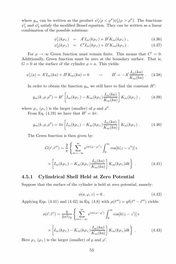
where gm can be written as the product ψ′1(ρ < ρ′′)ψ′

2(ρ > ρ′′). The functionsψ′

1 and ψ′2 satisfy the modified Bessel equation. They can be written as a linear

combination of the possible solutions:

ψ′1(kρ<) = A′Im(kρ<) +B′Km(kρ<) , (4.36)

ψ′2(kρ>) = C′Im(kρ>) +D′Km(kρ>) . (4.37)

For ρ → ∞ Green function must remain finite. This means that C′ = 0.Additionally, Green function must be zero at the boundary surface. That is,G = 0 at the surface of the cylinder ρ = a. This yields:

ψ′1(a) = A′Im(ka) +B′Km(ka) = 0 → B′ = −A′ Im(ka)

Km(ka). (4.38)

In order to obtain the function gm we still have to find the constant H ′:

gm(k, ρ, ρ′′) = H ′[

Im(kρ<) −Km(kρ<)Im(ka)

Km(ka)

]

Km(kρ>) , (4.39)

where ρ> (ρ<) is the larger (smaller) of ρ and ρ′′.From Eq. (4.19) we have that H ′ = 4π:

gm(k, ρ, ρ′′) = 4π

[

Im(kρ<) −Km(kρ<)Im(ka)

Km(ka)

]

Km(kρ>) . (4.40)

The Green function is then given by:

G(~r, ~r ′′) =2

π

∞∑

m=−∞eim(ϕ−ϕ′′)

∫ ∞

0

cos[k(z − z′′)]×

×[

Im(kρ<) −Km(kρ<)Im(ka)

Km(ka)

]

Km(kρ>)dk

. (4.41)

4.5.1 Cylindrical Shell Held at Zero Potential

Suppose that the surface of the cylinder is held at zero potential, namely:

φ(a, ϕ, z) = 0 . (4.42)

Applying Eqs. (4.41) and (4.42) in Eq. (4.8) with ρ(~r ′′) = qδ(~r ′ − ~r ′′) yields:

φ(~r, ~r ′) =q

2π2ε0

∞∑

m=−∞eim(ϕ−ϕ′)

∫ ∞

0

cos[k(z − z′)]×

×[

Im(kρ<) −Km(kρ<)Im(ka)

Km(ka)

]

Km(kρ>)dk

. (4.43)

Here ρ> (ρ<) is the larger (smaller) of ρ and ρ′.

53

Far from the origin, ρ is much larger than ρ′, hence we can express Eq. (4.43)in approximate form. The first term that appears between brackets is given byIm(kρ<)Km(kρ>), with ρ< = ρ′ and ρ> = ρ. Note the presence of the termKm(kρ), with ρ ≫ ρ′, which decays rapidly for increasing k. This implies thatthe main contribution of the integrand is in the region 0 < k < 1/ρ. Thenwe can approximate Im(kρ′) for small arguments, i.e., for kρ′ ≪ 1, yieldingIm(kρ′) ≈ (kρ′/2)m/m!. From this we can see that the most relevant term isthe first one, m = 0. The integral of the first term between brackets in Eq. (4.43)is then given by:

φ1(ρ≫ ρ′) ≈ q

2π2ε0

∫ ∞

0

cos[k(z − z′)]K0(kρ)dk =q

4πε0ρ. (4.44)

To arrive at the last equality we have used the identity given by [202, Prob. 11.5.11]:

2

π

∫ ∞

0

cos(xt)K0(yt)dt =1

√

x2 + y2. (4.45)

The second term that appears between brackets in Eq. (4.43) can be treated in asimilar way. The main contribution of the integrand is in the region 0 < k < 1/ρ.Again, the most relevant term is the first one. Accordingly, we approximate thefunction K0(kρ

′) for small arguments: K0(kρ′) ≈ − ln(kρ′). The integral of the

second term between brackets of Eq. (4.43) is then given by:

φ2(ρ ≫ ρ′) ≈ − q

2π2ε0

∫ ∞

0

cos[k(z − z′)]ln(kρ′)

ln(ka)K0(kρ)dk . (4.46)

From Eq. (4.43) the electric field is given by ~E0 = −∇φ, with components:

Eρ(ρ < ρ′) = − q

2π2ε0

∞∑

m=−∞eim(ϕ−ϕ′)

∫ ∞

0

k cos[k(z − z′)]×

×[

Im′(kρ) −K ′

m(kρ)Im(ka)

Km(ka)

]

Km(kρ′)dk

, (4.47)

Eρ(ρ > ρ′) = − q

2π2ε0

∞∑

m=−∞eim(ϕ−ϕ′)

∫ ∞

0

k cos[k(z − z′)]×

×[

Im(kρ′) −Km(kρ′)Im(ka)

Km(ka)

]

Km′(kρ)dk

, (4.48)

Eϕ =q

π2ε0ρ

∞∑

m=1

m sin[m(ϕ− ϕ′)]

∫ ∞

0

cos[k(z − z′)]×

×[

Im(kρ<) −Km(kρ<)Im(ka)

Km(ka)

]

Km(kρ>)dk

, (4.49)

Ez =q

2π2ε0

∞∑

m=−∞eim(ϕ−ϕ′)

∫ ∞

0

k sin[k(z − z′)]×

54

×[

Im(kρ<) −Km(kρ<)Im(ka)

Km(ka)

]

Km(kρ>)dk

. (4.50)

The zeroth order force ~F0 = q ~E0(~r′) acting upon the charge q is given by

Eq. (4.47) at ~r = ~r ′ without the first term between brackets (which is the fieldgenerated by the charge q itself). There is only a radial component:

~F0(~r′) =

q2

2π2ε0

[ ∞∑

m=−∞

∫ ∞

0

kKm(kρ′)Km′(kρ′)

Im(ka)

Km(ka)dk

]

ρ

= − q2

4π2ε0ρ′2

∞∑

m=−∞

∫ ∞

0

K2m(x)

d

dx

[

xIm(ax/ρ′)

Km(ax/ρ′)

]

dx

ρ . (4.51)

In the last equation we integrated by parts. We plot the zeroth order force ofEq. (4.51) in Fig. 4.3, normalized by the constant Fq ≡ q2/4πε0a

2, as a functionof ρ′/a. This force goes to zero when ρ′/a → ∞ and diverges when ρ′ → a, asexpected.

Figure 4.3: Zeroth order force F0 between an infinite grounded conductingcylinder of radius a and a point charge q at a distance ρ′ from the z axis(which is also the axis of symmetry of the cylinder), normalized by the constantFq ≡ q2/4πε0a

2. For ρ′ < a the force comes from Eq. (4.30), while for ρ′ > athe force is given by Eq. (4.51).

The surface charges can be calculated using Gauss’s law, yielding:

σ(a, ϕ, z) = ε0Eρ(a, ϕ, z) =

= − q

2π2a

[ ∞∑

m=−∞eim(ϕ−ϕ′)

∫ ∞

0

cos[k(z − z′)]Km(kρ′)

Km(ka)dk

]

. (4.52)

The charge per unit length λ(z) is given by:

λ(a, z) =

∫ 2π

0

σ(a, ϕ, z)a dϕ = − q

π

∫ ∞

0

cos[k(z − z′)]K0(kρ

′)

K0(ka)dk . (4.53)

55

It is interesting to obtain the behaviour of λ for a thin wire, far from z′

(|z − z′| ≫ ρ′ ≫ a). Utilizing Eq. (3.150) of Jackson’s book [13] we obtain:

λ ≈ − q

2 ln(|z|/a)1

√

ρ′2 + z2. (4.54)

The total charge induced in the cylinder can be obtained integrating Eq. (4.53)from z = −∞ to ∞. Utilizing Eq. (4.33) this yields:

Q =

∫ ∞

−∞λ(a, z)dz = −q . (4.55)

A plot of λ(a, z) as a function of z, with z′ = 0 and normalized by q/ρ′, isgiven in Fig. 4.4. The maximum value of λ(a, z) is given at z = z′, as expected.In Fig. 4.5 we plot λmax as a function of ρ′/a, normalized by q/ρ′. From thisFigure we can see that λmax → 0 when ρ′/a→ ∞, i.e., for a conducting cylinderof zero thickness, a simple conducting straight line.

Figure 4.4: Induced linear charge density λ on the conducting cylinder withan external point charge, Eq. (4.53), as a function of z/a. We utilized z′ = 0,ρ′/a = 2 and normalized by q/ρ′.

4.5.2 Thin Cylindrical Shell Held at Zero Potential

Consider that the grounded conducting cylinder is very thin, i.e., a ≪ ρ′. Themodified Bessel functions can be approximated for small argument by [203,Sec. 8.44]:

Im(y ≪ 1) ≈ 1

m!

ym

2m, (4.56)

Km(y ≪ 1) ≈ (m− 1)!2m−1

ym, m > 0 , (4.57)

K0(y ≪ 1) ≈ − lny

2− γ . (4.58)

56

Figure 4.5: Maximum induced linear charge density λmax(z = z′) on the con-ducting cylinder with an external point charge, Eq. (4.53), as a function of ρ′/a.We normalized the plot by q/ρ′.

Here γ = 0.577 is the Euler-Mascheroni constant.The term between brackets in Eq. (4.51) for m = 0 and for m > 0 can be

approximated by, respectively:

d

dx

[

x1

− ln ax2ρ′ − γ

]

≈ − 1

ln(a/ρ′), (4.59)

d

dx

[

x1

m!

(ax/ρ′)m

2m(ax/ρ′)m

(m− 1)!2m−1

]

≈ (2m+ 1)x2m(a/ρ′)2m

m!(m− 1)!22m−1. (4.60)

The most relevant term for ρ′ ≫ a is therefore m = 0. Utilizing the identity∫∞0 K2

0 (x)dx = π2/4 we have the zeroth order force acting upon the charge q asgiven by:

~F0(ρ′ ≫ a) ≈ − q2

4π2ε0ρ′2

∫ ∞

0

K20 (x)

ln(2ρ′/xa) − γ + 1

[γ − ln(2ρ′/xa)]2dxρ

≈ − q2

4π2ε0ρ′2 ln(ρ′/a)

∫ ∞

0

K20 (x)dxρ = − q2

16ε0ρ′2 ln(ρ′/a)

ρ . (4.61)

Alternatively, another expression for the force can be found by integratingthe force exerted by the linear charge density of a thin cylinder, λ(a, z) ofEq. (4.53), acting upon the point charge q. Utilizing that

∫ ∞

−∞

ρ′ cos[k(z − z′)]

[ρ′2 + (z − z′)2]3/2dz = 2kK1(kρ

′) , (4.62)

we obtain:

~F0(~r′) = − q

4πε0

∫ ∞

−∞

ρ′√

ρ′2 + z2

λ(a, z)

ρ′2 + z2dzρ

57

= − q2

2π2ε0ρ′2

∫ ∞

0

xK0(x)K1(x)

K0(xa/ρ′)dxρ . (4.63)

To compare Eqs. (4.61) and (4.63) we can expand the latter using the ap-proximation ρ′ ≫ a. Utilizing that K1(x) = −dK0/dx, integrating by parts,and using K0(xa/ρ

′) ≈ − ln(xa/2ρ′) − γ ≈ ln(ρ′/a) we obtain:

~F0 =q2

2π2ε0ρ′2

∫ ∞

0

xK0(x)(dK0/dx)

K0(xa/ρ′)dxρ

≈ − q2

4π2ε0ρ′

∫ ∞

0

K20 (x)

ln(2ρ′/xa) − γ + 1

[γ − ln(2ρ′/xa)]2dxρ

≈ − q2

16ε0ρ′2 ln(ρ′/a)

ρ , (4.64)

which is exactly Eq. (4.61).

4.5.3 Infinite Cylindrical Shell Held at Constant Potential

Suppose that the conducting cylinder is held at a constant potential, φ(a, ϕ, z) =φ0. From Eq. (4.41) we obtain (with n′′ = ρ< and ρ> = ρ):

∂G

∂n′′

∣

∣

∣

∣

∣

ρ′′=a

= − 2

π

∞∑

m=−∞eim(ϕ−ϕ′′)

∫ ∞

0

k cos[k(z − z′′)]Km(kρ)

Km(ka)×

×[

Im′(kρ′′)Km(ka) − Im(ka)Km

′(kρ′′)]

dk

ρ′′=a

=2

πa

∞∑

m=−∞eim(ϕ−ϕ′′)

∫ ∞

0

cos[k(z − z′′)]Km(kρ)

Km(ka)dk

. (4.65)

In the last equality we utilized the Wronskian relation W [Im(kρ′′),Km(kρ′′)] =−1/(kρ′′).

The second term given by Eq. (4.8) can be written as:

φ+ = − 1

4π©∫∫

S

φ(~r ′′)∂G

∂n′′ da′′ =

φ0

2π2a

∫ ∞

−∞a dz′′

∫ 2π

0

dϕ′′×

× ∞∑

m=−∞eim(ϕ−ϕ′)

∫ ∞

0

cos[k(z − z′)]Km(kρ)

Km(ka)dk

=φ0

π

∫ ∞

−∞dz′′

∫ ∞

0

cos[k(z − z′)]K0(kρ)

K0(ka)dk

=2φ0

π

∫ ∞

0

dz′′∫ ∞

0

cos[k(z − z′)]K0(kρ)

K0(ka)dk . (4.66)

58

In the last equality we changed the limits of the integral over z′′.In order to calculate the last integral, we utilize Eq. (4.23). Changing vari-

ables, we have:∫ ∞

0

cos[k(z − z′)]dz′ = πδ(k) . (4.67)

The approximation for small argument of K0(y), namely, K0(y) ≈ − ln y, is inthis case inappropriate, because the term limk→0K0(kρ)/K0(ka) → 1 for anyρ. This is true for an infinite cylinder, but gives no physical insight into thebehaviour of the potential as a function of ρ. We should use instead k ≪ 1/ρ <1/a, yielding:

φ+ ≈ φ0ln(kρ)

ln(ka), for k ≪ 1/ρ < 1/a . (4.68)

The potential outside an infinite conducting cylinder with an external charge,held at a constant potential φ0, is then given by the summation of Eqs. (4.43)and (4.68).

We can find the potential of a cylinder held at a constant potential φ0 bya different method. Suppose we have a long straight line of length ℓ along thez axis, uniformly charged with a linear charge density λ. The potential at adistance ρ from the z axis, for ℓ≫ ρ, is given by:

φline ≈ λ

2πε0lnℓ

ρ. (4.69)

At a distance ρ = a from the z axis, we have a constant potential φ0 =2λ ln(ℓ/a), which is the same boundary condition as before. This implies thatthe solution is the same. Substituting λ, we obtain the potential as given by:

φline = φ0ln(ℓ/ρ)

ln(ℓ/a). (4.70)

Note that Eq. (4.68) with k ≪ 1/ρ < 1/a and Eq. (4.70) with ℓ ≫ a > ρ areessentially the same. Henceforth, we utilize Eq. (4.70) as the solution for a longcylinder held at a constant potential.

The final potential of the problem of a long conducting cylinder held at aconstant potential φ0 with an external charge q is given by:

φ(~r, ~r ′) =q

2π2ε0

∞∑

m=−∞eim(ϕ−ϕ′)

∫ ∞

0

cos[k(z − z′)]Km(kρ>)×

×[

Im(kρ<) − Im(ka)

Km(ka)Km(kρ<)

]

dk

+ φ0ln(ℓ/ρ)

ln(ℓ/a). (4.71)

The components of the zeroth order electric field ~E0, the zeroth order force ~F0

exerted on q, the surface charge density σ and the linear charge density λ aregiven by, respectively:

Eρ(ρ < ρ′) = − q

2π2ε0

∞∑

m=−∞eim(ϕ−ϕ′)

∫ ∞

0

k cos[k(z − z′)]×

59

×[

Im′(kρ) − Im(ka)

Km(ka)K ′m(kρ)

]

Km(kρ′)dk

, (4.72)

Eρ(ρ > ρ′) = − q

2π2ε0

∞∑

m=−∞eim(ϕ−ϕ′)

∫ ∞

0

k cos[k(z − z′)]×

×[

Im(kρ′) − Im(ka)

Km(ka)Km(kρ′)

]

Km′(kρ)dk

+φ0

ρ ln(ℓ/a), (4.73)

Eϕ =q

π2ε0ρ

∞∑

m=1

m sin[m(ϕ− ϕ′)]

∫ ∞

0

cos[k(z − z′)]×

×[

Im(kρ<) − Im(ka)

Km(ka)Km(kρ<)

]

Km(kρ>)dk

, (4.74)

Ez =q

2π2ε0

∞∑

m=−∞eim(ϕ−ϕ′)

∫ ∞

0

k sin[k(z − z′)]×

×[

Im(kρ<) − Im(ka)

Km(ka)Km(kρ<)

]

Km(kρ>)dk

, (4.75)

~F0(~r′) = − q2

4π2ε0ρ′2

∞∑

m=−∞

∫ ∞

0

K2m(x)

d

dx

[

xIm(ax/ρ′)

Km(ax/ρ′)

]

dx

ρ

+qφ0

ρ′ ln(ℓ/a)ρ , (4.76)

σ(a, ϕ, z) = − q

2π2

∞∑

m=−∞eim(ϕ−ϕ′)

∫ ∞

0

k cos[k(z − z′)]Km(kρ′)

Km(ka)dk

+ε0φ0

a ln(ℓ/a), (4.77)

λ(a, z) = − q

π

∫ ∞

0

cos[k(z − z′)]K0(kρ

′)

K0(ka)dk +

2πε0φ0

ln(ℓ/a). (4.78)

From Eq. (4.78) we can calculate the total charge on the cylinder:

Q =

∫ ∞

−∞λ(a, z)dz = − q

π

∫ ∞

−∞dz

∫ ∞

0

cos[k(z − z′)]K0(kρ

′)

K0(ka)dk +

2πℓε0φ0

ln(ℓ/a)

= −q limk→0

ln(kρ′)

ln(ka)+

2πℓε0φ0

ln(ℓ/a)= −q +

2πℓε0φ0

ln(ℓ/a). (4.79)

For a neutral charged cylinder, i.e., Q = 0, we can relate the constant potentialφ0 with the charge q by:

φ0 =q ln(ℓ/a)

2πε0ℓ. (4.80)

60

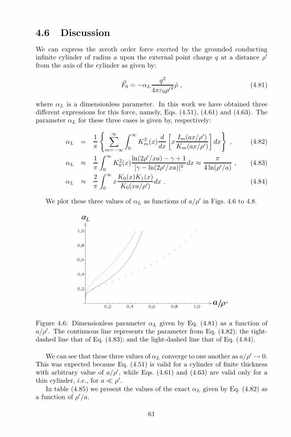
4.6 Discussion

We can express the zeroth order force exerted by the grounded conductinginfinite cylinder of radius a upon the external point charge q at a distance ρ′

from the axis of the cylinder as given by:

~F0 = −αLq2

4πε0ρ′2 ρ , (4.81)

where αL is a dimensionless parameter. In this work we have obtained threedifferent expressions for this force, namely, Eqs. (4.51), (4.61) and (4.63). Theparameter αL for these three cases is given by, respectively:

αL =1

π

∞∑

m=−∞

∫ ∞

0

K2m(x)

d

dx

[

xIm(ax/ρ′)

Km(ax/ρ′)

]

dx

, (4.82)

αL ≈ 1

π

∫ ∞

0

K20(x)

ln(2ρ′/xa) − γ + 1

[γ − ln(2ρ′/xa)]2dx ≈ π

4 ln(ρ′/a), (4.83)

αL ≈ 2

π

∫ ∞

0

xK0(x)K1(x)

K0(xa/ρ′)dx . (4.84)

We plot these three values of αL as functions of a/ρ′ in Figs. 4.6 to 4.8.

Figure 4.6: Dimensionless parameter αL given by Eq. (4.81) as a function ofa/ρ′. The continuous line represents the parameter from Eq. (4.82); the tight-dashed line that of Eq. (4.83); and the light-dashed line that of Eq. (4.84).

We can see that these three values of αL converge to one another as a/ρ′ → 0.This was expected because Eq. (4.51) is valid for a cylinder of finite thicknesswith arbitrary value of a/ρ′, while Eqs. (4.61) and (4.63) are valid only for athin cylinder, i.e., for a≪ ρ′.

In table (4.85) we present the values of the exact αL given by Eq. (4.82) asa function of ρ′/a.

61

Figure 4.7: Dimensionless parameter αL given by Eq. (4.81) as a function ofa/ρ′, for the region a/ρ′ ≪ 1. The continuous line represents the parameter fromEq. (4.82); the tight-dashed line represents the parameter of Eq. (4.83); and thelight-dashed line (which in this interval of a/ρ′ is overlaid on the continuousline) represents the parameter of Eq. (4.84).

Figure 4.8: Dimensionless parameter αL given by Eq. (4.81) as a function oflog10(a/ρ

′), for the region a/ρ′ ≪ 1. The continuous line represents the parame-ter from Eq. (4.82); the tight-dashed line represents the parameter of Eq. (4.83);and the light-dashed line (which in this interval of a/ρ′ is overlaid on the con-tinuous line) represents the parameter of Eq. (4.84).

From Eq. (4.83) we can see that when a/ρ′ ≪ 1, the parameter αL behavesas π/[4 ln(ρ′/a)]. That is, it goes to zero when a/ρ′ → 0. According to thesecalculations we conclude that there is no force between a point charge andan idealized grounded conducting line (of zero thickness). One of the authors(AKTA) [1] had expected 0 < αL < 1, not specifically for a grounded conductingline, but for a conducting line with zero total charge. In particular he expectedthat 0.1 < αL < 0.9, by guessing the result based on dimensional analysis andin analogy with the case of a point charge q at a distance ρ′ from an infinite

62

conducting plane. In this last case, the net force upon the test charge is given byαP q

2/4πε0ρ′2, with αP = 1/4 = 0.25. The results of the calculations presented

here, on the other hand, indicate that αL = 0 when a/ρ′ = 0 (in the case of agrounded infinite line). This is an interesting result indicating that the existenceof a force upon the external test charge requires not only that it is at a finitedistance to the cylinder, but also the existence of a surface area different fromzero in the conductor with which it is interacting.

ρ′/a αL1.1 29.11.2 8.941.5 2.202.0 0.9445 0.32210 0.228100 0.130103 0.0930104 0.07271010 0.0318

(4.85)

Later on we compare this zeroth order force with the force proportionalto the voltage of the battery arising when a constant current flows upon thecylindrical wire.

63

64

Chapter 5

Relevant Topics

5.1 Properties of the Electrostatic Field

We present here some properties of the scalar electric potential, φ, and of theelectric field, ~E. These properties are proved in detail in most books dealingwith electromagnetism, so that we present here only the main aspects. Supposethat we are in an inertial frame of reference S with origin 0. There are Npoint charges qj at rest in this reference frame, with j = 1, ..., N . The positionvector describing the location of charge qj relative to 0 is represented by ~rj .The electric potential at the point ~ro due to these N charges, according to theprinciple of superposition, is defined by:

φ(~ro) ≡N∑

j=1

qj4πε0

1

roj, (5.1)

where roj ≡ |~ro − ~rj | is the distance between the tip of the vector ~ro and thecharge qj .

The electric field at the point ~ro is given by

~E(~ro) = −∇oφ . (5.2)

Performing the line integral between points A and B of the potential differ-ence, dφ = − ~E · d~ℓ, yields

∫ B

A

~E · d~ℓ = −∫ B

A

(∇φ) · d~ℓ = −∫ B

A

dφ = φ(~rA) − φ(~rB) . (5.3)

That is, this integral is independent of the path of integration, being afunction only of the initial and final points.

If it is performed an integration around a closed path of arbitrary form, thisyields a null value:

∮

~E · d~ℓ = 0 . (5.4)

65

5.2 The Electric Field in Different Points of the

Cross-section of the Wire

Let us suppose a rectilinear, resistive and homogeneous wire, of uniform cross-section, conducting a steady current. It seems that Davy was the first to provein 1821 that the current flows over the whole cross-section and not only alongthe surface of the wire [63, p. 90]:

As we have already seen, Cavendish investigated very completelythe power of metals to conduct electrostatic discharges; their powerof conducting voltaic currents was now examined by Davy.1 Hismethod was to connect the terminals of a voltaic battery by a pathcontaining water (which it decomposed), and also by an alterna-tive path consisting of the metallic wire under examination. Whenthe length of the wire was less than a certain quantity, the waterceased to be decomposed; Davy measured the lengths and weightsof wires of different materials and cross-sections under these limitingcircumstances; and, by comparing them, showed that the conduct-ing power of a wire formed of any one metal is inversely proportionalto its length and directly proportional to its sectional area, but in-dependent of the shape of the cross-section.2 The latter fact, as heremarked, showed that voltaic currents pass through the substanceof the conductor and not along its surface.

A theoretical proof that the current fills the cross-section of the wire canbe found in the book of Chabay and Sherwood [166, Section 18.2.4, p. 631].Suppose there is a solid, homogeneous, rectilinear and uniformly resistive wire,with a cross-section of arbitrary form, carrying a steady current. In steady-state the electric field must be parallel to the wire (to avoid transverse currentsand transverse electrostatic polarizations). Imagine now a rectangular pathABCDA within the wire, with AB and CD parallel to the wire, while BC andDA are perpendicular to the wire. When we perform the line integration of theelectric field, we get a null value, as was shown in Section 5.1. In this proof weutilized charges at rest. In the case of this Section we are considering steadycurrents, so that the surface charges are also moving with a drifting velocity ofvalue vd relative to the bulk of the wire. But these drifting velocities are verysmall compared to light velocity c. This means that the corrections of secondorder, of the type v2

d/c2, will be negligible in comparison to Coulomb’s force.

Therefore, they will not be considered here. This means that the electric fieldin the section AB must be parallel to the wire, with its intensity equal to theintensity of the electric field in the section CD. By the microscopic form ofOhm’s law we find that the same result must be true for the volume currentdensity, ~J .

1Phil. Trans. cxi (1821), p. 425. His results were confirmed by Becquerel, Annales de

Chimie, xxxii (1825), p. 423.2These results had been known to Cavendish.

66

Even with the component of the electric field arising from the radial Halleffect, to be discussed in Section 6.4, the same result will be maintained. Thereason for this is that the component of the electric field pointing toward theaxis of the wire will have its line integral cancelled between the sections BC andDA.

Utilizing the same reasoning in the case of a circuit having the shape of asolid and homogeneous ring, conducting an azimuthal current, we find that theazimuthal electric field (neglecting the small radial Hall effect) must decreaseas 1/ρ, where ρ is the distance of the observation point to the ring axis ofsymmetry. We will see an example of this fact in Chapter 13.

We do not know any experience which tried to verify if the electric field andvolume current density are really constants in all points of the cross-section ofa metallic rectilinear wire carrying a steady current. The same can be said ofthe 1/ρ dependence in the case of a ring. But the experiences of Bergman,Schaefer, Jefimenko and Parker (see Chapter 3) show qualitatively that thesesuppositions are reasonable.

5.3 Electromotive Force Versus Potential Differ-

ence

In this book we will see several examples showing that the electric field outsidea wire carrying a steady current is proportional to the electromotive force (emf)of the battery connected to the wire. In this Section we emphasize that the emfis a concept different from the potential difference due to charges at rest. Thistopic has been discussed by a number of authors [204] [16, Section 7.1.2, pp.277-278] [171] [166, pp. 642-644].

In order to separate positive and negative charges it is necessary the existenceof “non-Coulomb” forces, ~FnC , i.e., forces which are not of electrostatic origin.This must happen in all cases in which we separate these charges: in frictionalelectricity; when two different metals touch one another; in a chemical battery;in thermoelectric effect; in piezoelectric effect; in a Van de Graaff generator;in a photoelectric cell, etc. The reason for this is that due to Coulomb’s force,charges of opposite sign attract one another and tend to get together. Whatseparate these charges (or prevent them from getting together once they wereseparated) can then only be of non-electrostatic origin. That is, this interactionmust be independent from Coulomb’s electrostatic force.

The origin of the expression “electromotive force” is due to Volta (1745-1827)[204].

As we have seen in Section 5.1, the difference of electrostatic potential be-tween two points A and B is given by

φB − φA = −∫ B

A

~EC · d~ℓ . (5.5)

Here ~EC is the electrostatic field due to charges at rest. This potential difference

67

does not depend upon the path of integration, being a function only of the initialand final points.

On the other hand, the electromotive force between two points A and B,emfBA, is given by

emfBA =

∫ B

A

~EnC · d~ℓ . (5.6)

Here ~EnC = ~FnC/q is the impressed force acting upon the test charge q, dividedby the value of this charge. This impressed force has a non-electrostatic origin.This line integral depends upon the path of integration.

In a battery, for instance, the Coulomb and non-Coulomb forces balance oneanother in an open circuit. This means that there will be a potential differenceacross the battery. Moreover, this potential difference is numerically equal tothe battery’s emf. The emf of a battery is also called its voltage.

Analogously, the emf of a closed circuit is given by:

emf =

∮

~EnC · d~ℓ . (5.7)

If in the closed circuit there is a chemical battery, or another force of non-electrostatic origin, this line integral upon a closed circuit may have a net valuedifferent from zero.

Despite the term “force” in the expression emf, the emf is not a force in theNewtonian sense. The emf of a pile or chemical battery is numerically equal tothe potential difference generated between the terminals of the battery. It hasthe same units as potential difference, namely, volt or newton/coulomb. Despitethis fact, the emf is not a potential difference, as we emphasized in this Section.Its origin is due to a non-electrostatic force. And it is not always associated witha potential difference. For instance, in the case of a ring approaching or movingaway from a permanent magnet (example discussed by Weber, as we discuss inAppendix A), it is generated a current along the resistive ring, although thereis no potential difference between any two points of the ring [204] [184].

5.4 Russell’s Theorem

Russell proved in an important short paper a general theorem related withstraight parallel conductors of arbitrary cross-sections carrying steady currents[9]. He concluded that the density of surface charges σ on the conductors varylinearly with distance along the direction of their common axis z. The samewas found valid for the potential φ inside and outside the conductors.

He considered homogeneous isotropic materials surrounded by an insulatingmedium of constant permittivity ε. His theorem is valid at great distances fromtheir termination (in order to neglect edge effects) and also far from the sourcesof electromotive force, emf, maintaining the current.

68

The essence of his proof is to consider that inside the conductors carryingsteady currents the electric field ~E has everywhere the same longitudinal compo-nent. By ~E = −∇φ this means that the potential inside them must be a linearfunction of z. Outside the conductors the potential φ must satisfy Laplace’sequation ∇2φ = 0. But the solutions of Laplace’s equation which satisfy all theboundary conditions are unique. As the boundary conditions in all conductorsare linear functions of z, the same must be true outside them. That is,

φ(x, y, z) = F (x, y)(A+Bz) , (5.8)

where F (x, y) is a function of the transverse coordinates, while A and B areconstants.

Analogously, the surface charge densities σ are obtained by Gauss’s lawas directly proportional to the normal component of the electric field at theconductor boundaries. As ~E = −∇φ, Eq. (5.8) yields:

σ(x, y, z) = G(x, y)(A +Bz) , (5.9)

where G(x, y) is a function of the transverse coordinates.This means that the solution of electrostatic problems can be directly ap-

plied to the solution of steady currents, by including a linear dependence in thelongitudinal component. In the following Chapters we will see many examplesillustrating this theorem.

But it should be kept in mind that it is valid only far from the terminationsof the conductors and also far from the batteries. Moreover, it is not valid aswell close to the junction of two materials of different conductivities.

69

70

Part II

Straight Conductors

71

In this work the frame of reference will always be the laboratory. When wespeak of conductors and wires in general, it should be understood that they areusually uniformly resistive, unless stated otherwise. The medium outside theconductors or between them will be usually air or vacuum. No time variation ofcurrents or potentials will be considered here. It is assumed that there are noconductors nor other external charges close to the current-carrying wire, so thatwe will consider it isolated from external influences (except for the test chargealready mentioned).

In this first part we will consider one or more parallel resistive conductorscarrying steady currents along the z axis.

73

74

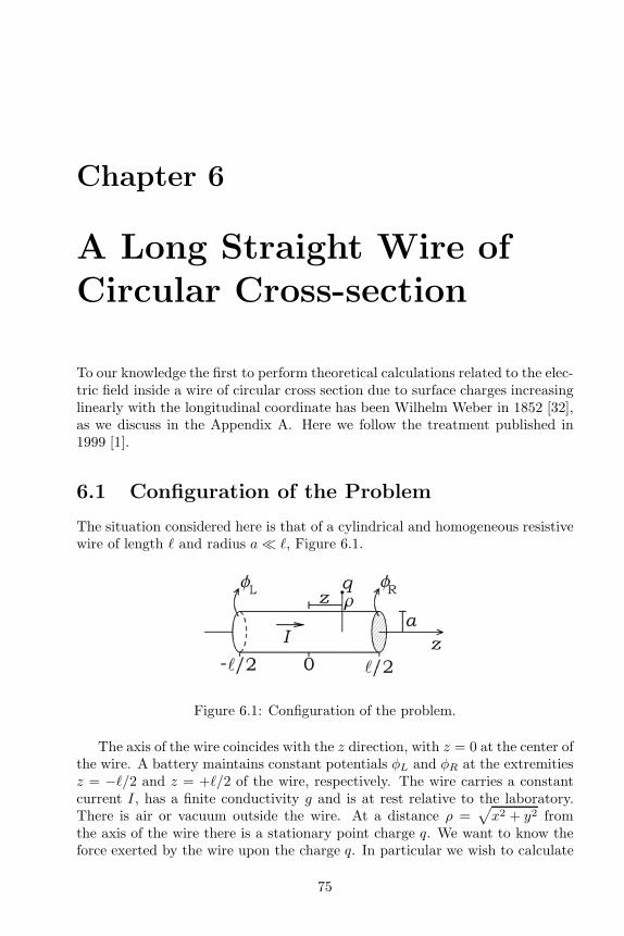
Chapter 6

A Long Straight Wire of

Circular Cross-section

To our knowledge the first to perform theoretical calculations related to the elec-tric field inside a wire of circular cross section due to surface charges increasinglinearly with the longitudinal coordinate has been Wilhelm Weber in 1852 [32],as we discuss in the Appendix A. Here we follow the treatment published in1999 [1].

6.1 Configuration of the Problem

The situation considered here is that of a cylindrical and homogeneous resistivewire of length ℓ and radius a≪ ℓ, Figure 6.1.

Figure 6.1: Configuration of the problem.

The axis of the wire coincides with the z direction, with z = 0 at the center ofthe wire. A battery maintains constant potentials φL and φR at the extremitiesz = −ℓ/2 and z = +ℓ/2 of the wire, respectively. The wire carries a constantcurrent I, has a finite conductivity g and is at rest relative to the laboratory.There is air or vacuum outside the wire. At a distance ρ =

√

x2 + y2 fromthe axis of the wire there is a stationary point charge q. We want to know theforce exerted by the wire upon the charge q. In particular we wish to calculate

75

the component of this force which is proportional to the voltage or emf of thebattery, or to the potential difference acting along the wire. To this end we willsuppose the following approximation:

ℓ≫ ρ ≥ 0, ℓ≫ a > 0 and ℓ≫ |z| ≥ 0 . (6.1)

Here z is the longitudinal component of the vector position of q. See Fig. 6.1. Weutilize throughout this chapter cylindrical coordinates (ρ, ϕ, z) and unit vectorsρ, ϕ and z.

This wire must be closed somewhere. The calculations presented here withthis approximation should be valid for the circuit of Figure 6.2. This is a squarecircuit with four sides of length ℓ, composed of cylindrical wires of radius a≪ ℓ.There is an external point charge close to the middle of one of its sides (likeAB, BC or CD) and far from the battery. The case when the point charge isclose to the middle of the side AD has been published in 2004 [205].

Figure 6.2: A closed square circuit made of a resistive wire of circular cross-section. There is a point charge close to the middle of one of its sides.

With this approximation we can consider that the three other sides will notcontribute significantly to the potential and field near the center of the fourthside. Alternatively, it should also give approximate results for a circular loop oflarger radius R0 = ℓ/2π and smaller radius a≪ R0 (a ring), if the point chargeis close to the ring but far from the battery maintaining the current. It mighteven be utilized as a first gross approximation for the force on the point chargeof Figure 1.1 considering a generic circuit of large length and small curvatures(that is, with radii of curvature much larger than the diameter of the wire andalso much larger than the distance of the point charge to the wire).

We consider separately three components of the force exerted by the wireon q: (A) The component due to the electrostatic induction, based upon thecharges induced along the surface of the wire by q, which has been considered inChapter 4; (B) the component of the force due to the surface charges which existin resistive wires carrying steady currents (force proportional to the voltage oremf of the battery connected to the circuit); and (C) the force proportional to the

76

square of the drifting velocity, vd, of the conduction electrons, i.e., proportionalto v2

d/c2.

6.2 Force Proportional to the Potential Differ-

ence Acting upon the Wire

When a constant current flows in a resistive wire connected to a battery, the elec-tric field driving the conduction electrons against the resistive friction exertedupon them by the lattice is due to free charges distributed along the surface ofthe wire, as we have seen before. We represent this surface charge density byσ(a, ϕ, z). For steady currents, σ is constant in time but varies along the lengthof the wire (that is, it is a function of z). Here we follow the approach of Weberand Kirchhoff discussed in Chapter 2. The battery, due to the chemical forceswhich maintain its terminals at different potentials, is responsible for maintain-ing this distribution of charges along the surface of the wire. But the batterydoes not generate directly the electric field in all points along the circuit. Thesurface charges, on the other hand, generate not only the electric field insidethe wire but also an electric field outside it.

The approach of this chapter is the following: We consider the cylindricalwire carrying the constant current I and calculate the potential φ1 and electricfield ~E1 inside and outside the wire due to these surface charges in the absenceof the test charge q. When we put the test charge at a distance ρ from thewire the force on it due to the surface charges will be then given by ~F1 = q ~E1,supposing that it is small enough such that it does not disturb the current northe wire (except from the induction charges already considered in Chapter 4,

which will exert the force ~F0 = q ~E0). We begin calculating the potential due tothe surface charges.

As there is a constant current in the wire, the electric field inside it anddriving the current must be constant over the cross-section of the wire [63, p.90]. Here we are disregarding the small radial Hall effect inside the wire due tothe azimuthal magnetic field generated by the current to be discussed in Section6.4. This means that the potential and surface charge distribution must be alinear function of z, as we saw in Section 5.4. Due to the axial symmetry of thewire it cannot depend on the azimuthal angle either. This means that

σ(a, ϕ, z) = σA + σBz

ℓ, (6.2)

where σA and σB are constants.Before proceeding we wish to discuss this expression. We may wish to con-

sider the wire as globally neutral, i.e., no net charge as a whole. When weintegrate the free charge density σ over the whole surface of the wire we needto obtain a zero net value in this case. This will happen with Eq. (6.2) afterintegrating from z = −ℓ/2 to z = ℓ/2 only in the symmetrical case in whichσA = 0. This might represent, for instance, the top side BC of Figure 6.2. Onthe other hand, we will perform the calculations with a generic value of σA so

77

that the calculation might be applicable, for instance, to the left half of the topside BC of Figure 6.2. The integration of σ over this left side (from z = −ℓ/2to zero) will yield a positive value, as it is closer to the positive terminal. Thispositive charge will be balanced by the negative charge lying on the right halfof the top side of Figure 6.2 (z going from zero to +ℓ/2). With a generic σA wemight also consider, for instance, the left side AB of Figure 6.2 with a positivecharge, which will be balanced by the negative charge in the right side CD ofFigure 6.2. It should be emphasized that the point where σ = 0 is specified bythe battery. The battery itself also specifies where σ will be positive (portions ofthe wire closer to its positive terminal) or negative (portions of the wire closerto its negative terminal).

Due to the axial symmetry of σ we can calculate φ at the specific angle ϕ = 0rad and then generalize the solution to all ϕ. The potential inside or outsidethe wire is then given by:

φ1(ρ, z) =1

4πε0

∫ 2π

ϕ2=0

∫ ℓ/2

z2=−ℓ/2

σadϕ2dz2√

ρ2 + a2 − 2ρa cosϕ2 + (z2 − z)2

=1

4πε0

∫ 2π

ϕ2=0

∫ ℓ/2

z2=−ℓ/2

(σA + σBz2/ℓ)dϕ2dz2√

(

1 − 2 ρa cosϕ2 + ρ2

a2

)

+(

z2−za

)2. (6.3)

Defining the dimensionless variables s2 ≡ 1−2(ρ/a) cosϕ2+(ρ2/a2) and u ≡(z2 − z)/a we are then led to: φ1(ρ, z) = (a/4πε0)[(σBa/ℓ)I1 +(σA+σBz/ℓ)I2],where

I1 ≡∫ 2π

ϕ2=0

∫ ℓ/2a−z/a

u=−(ℓ/2a+z/a)

udϕ2du√s2 + u2

, (6.4)

and

I2 ≡∫ 2π

ϕ2=0

∫ ℓ/2a−z/a

u=−(ℓ/2a+z/a)

dϕ2du√s2 + u2

. (6.5)

These integrals can be solved with the approximation (6.1). The final ap-proximate result is given by (generalizing for all ϕ):

φ1(ρ ≤ a, ϕ, z) ≈ a

ε0

[

σA lnℓ

a+ σB

z

ℓln

ℓ

ea

]

, (6.6)

φ1(ρ ≥ a, ϕ, z) ≈ a

ε0

[

σA lnℓ

ρ+ σB

z

ℓln

ℓ

eρ

]

. (6.7)

From Eq. (6.1) we can neglect ln e = 1 in comparison with ln(ℓ/a) andln(ℓ/ρ). This yields:

φ1(ρ, ϕ, z) ≈aσ(z)

ε0lnℓ

a=a(σA + σBz/ℓ)

ε0lnℓ

a, if ρ ≤ a , (6.8)

78

φ1(ρ, ϕ, z) ≈aσ(z)

ε0lnℓ

ρ=a(σA + σBz/ℓ)

ε0lnℓ

ρ, if ρ ≥ a . (6.9)

By writing the linear density of charges along the wire as λ(z) ≡ 2πaσ(z)these last expressions can be written as

φ1(ρ ≤ a, ϕ, z) ≈ λ(z)

2πε0lnℓ

a, (6.10)

φ1(ρ ≥ a, ϕ, z) ≈ λ(z)

2πε0lnℓ

ρ. (6.11)

From Eqs. (6.6) and (6.7) we can obtain the electric field ~E1 = −∇φ1:

~E1(ρ < a, ϕ, z) ≈ −aσBε0ℓ

(

lnℓ

ea

)

z , (6.12)

~E1(ρ > a, ϕ, z) ≈ a

ε0

(

σA + σBz

ℓ

) ρ

ρ− aσB

ε0ℓ

(

lnℓ

eρ

)

z . (6.13)

To our knowledge the first to obtain Eq. (6.12) beginning with the integrationof Eq. (6.2) was Wilhelm Weber in 1852, as we discuss in Appendix A.

From Eq. (6.1) we can neglect 1 in comparison with ln(ℓ/a) and ln(ℓ/ρ).This yields the coulombian force on a test charge q located at (ρ, ϕ, z) as given

by (with ~F1 = −q∇φ1):

~F1 = q ~E1 ≈ −qaε0

∂σ(z)

∂z

(

lnℓ

a

)

z = −qaσBℓε0

(

lnℓ

a

)

z if ρ < a , (6.14)

~F1 = q ~E1 ≈ qaσ(z)

ε0

ρ

ρ− qa

ε0

∂σ(z)

∂z

(

lnℓ

ρ

)

z

=qa(σA + σBz/ℓ)

ε0

ρ

ρ− qaσB

ℓε0

(

lnℓ

ρ

)

z if ρ > a . (6.15)

We can relate these expressions with the current I flowing in the wire. FromFigure 6.1 and the fact that φ1 is a linear function of z we obtain

φ1(ρ ≤ a, z) =φR + φL

2+ (φR − φL)

z

ℓ. (6.16)

Equating this with Eq. (6.8) and utilizing Ohm’s law φL − φR = RI,where R = ℓ/gπa2 is the resistance of the wire, with g being its conductiv-ity, yields σB = −Rε0I/a ln(ℓ/a) and σA = ε0(φR + φL)/2a ln(ℓ/a) = ε0(RI +2φR)/2a ln(ℓ/a). The density of free charges along the surface of the wire canthen be written as:

79

σ(a, ϕ, z) =ε0(φR + φL)

2a ln(ℓ/a)− Rε0I

a ln(ℓ/a)

z

ℓ. (6.17)

This means that the potential and the force on the test charge q are given by:

φ1 =φR + φL

2−RI

z

ℓif ρ ≤ a , (6.18)

φ1 =φR + φL

2

ln(ℓ/ρ)

ln(ℓ/a)−RI

ln(ℓ/ρ)

ln(ℓ/a)

z

ℓif ρ ≥ a , (6.19)

~F1 = q ~E1 = qRI

ℓz if ρ < a , (6.20)

~F1 = q ~E1 = q

[

1

ln(ℓ/a)

(

RI + 2φR2

−RIz

ℓ

)

ρ

ρ+RI

ℓ

ln(ℓ/ρ)

ln(ℓ/a)z

]

if ρ > a .

(6.21)Now that we have obtained the potential outside the wire we might also

invert the argument. That is, we might solve Laplace’s equation ∇2φ = 0in cylindrical coordinates inside and outside the wire (for a ≤ ρ ≤ ℓ) by themethod of separation of variables, supposing a solution of the form φ(ρ, ϕ, z) =R(ρ)Φ(ϕ)Z(z). The arbitrary constants obtained by this method are foundimposing the following boundary conditions: finite φ(0, ϕ, z), φ(a, ϕ, z) = (φR+φL)/2 + (φR − φL)z/ℓ and φ(ℓ, ϕ, z) = 0. This last condition is not a trivialone and was obtained only after we found the solution in the order presentedin this work. See Eq. (6.9). The usual boundary condition that the potentialgoes to zero at infinity does not work in the case of a long cylinder carrying asteady current. But the potential going to zero at ρ = ℓ is a reasonable result.After all, this means that we are considering φ = 0 at a great distance fromthe wire. By this reverse method we obtain the potential inside and outside thewire, then the electric field by ~E = −∇φ and lastly the surface charge densityby ε0 times the normal component of the electric field outside the wire in thelimit in which ρ→ a. In this way we checked the calculations.

If we put φL = φR = φ0 or I = 0 in Eqs. (6.18) to (6.21) we recoverthe electrostatic solution (long wire charged uniformly with a constant chargedensity σA, with total charge QA = 2πaℓσA), namely:

φ1(ρ ≤ a) = φ0 =aσAε0

lnℓ

a, (6.22)

φ1(ρ ≥ a) = φ0ln(ℓ/ρ)

ln(ℓ/a)=aσAε0

lnℓ

ρ, (6.23)

~E1(ρ < a) = ~0 , (6.24)

~E1(ρ > a) =φ0

ln(ℓ/a)

ρ

ρ=aσAε0

ρ

ρ. (6.25)

80

We can also obtain the capacitance per unit length of this long cylindrical wireas C/ℓ = [QA/φ(a)]/ℓ = 2πε0/ ln(ℓ/a).

It is interesting to analyze here the solutions for points extremely close tothe wire, ρ = a+ d with d≪ a. In this approximation Eq. (6.9) yields:

φ1 ≈ aσ(z)

ε0

(

lnℓ

a− d

a

)

. (6.26)

The analysis presented here refines the previous work of Coombes and Laue,who discussed in 1981 the limiting case of an infinitely long wire [17]. Theyarrived at the same uniform electric field both inside and outside the wire.This is correct for an infinitely long wire. In the present case we arrived at auniform electric field inside the wire and at an electric field outside the wire withlongitudinal and radial components depending on ρ, as we were considering alarge but finite length ℓ.

Eqs. (6.16), (6.20) and (6.21) show that the electric field both inside andoutside the wire is proportional to the potential difference φL−φR = RI actingalong the wire. The same can be said of the force exerted upon a stationaryexternal test charge by the resistive wire carrying a steady current. If we changethe diameter of the wire, or its resistivity, we can change the resistance of thewire. But if it is connected to the same battery, in such a way that it is underthe action of the same potential difference, the current flowing along the wirewill change accordingly. But the density of surface charges and the externalelectric field will not change. This important aspect has been emphasized byChabay and Sherwood [165, 166, 171].

Moreover, there will be not only a tangential component of the electric fieldoutside the wire (as might be expected from the continuity of this componentat an interface between two media), but also a radial component. In the sym-metrical case in which φL = −φR = RI/2 the ratio of the radial component of~F1 to its tangential component is given by z/[ρ ln(ℓ/ρ)]. For a wire with 1 meterlength with z = ρ = 10 cm this ratio is given by 0.4. This means that these twocomponents are of the same order of magnitude.

The longitudinal component of the electric field is continuous at an interfaceseparating two media. From Eqs. (6.20) and (6.21) we can see that at the surfaceof the wire, ρ = a, the longitudinal component of the electric field is given by:~E1 = (RI/ℓ)z. This electric field will act upon the surface conduction electronsbelonging to the wire, so that they will move with a constant tangential velocityin steady state, with the electric force balanced by the Ohmic resistance. Inequilibrium there will be the same number of free electrons entering and leavinga circular strip of length 2πa and width dz, so that the distribution of surfacecharges will not change with time, although being a function of z. In any event,the surface charges will not remain stationary when there is a steady current,but will move due to this tangential electric field existing at the surface of theconductor. The drifting velocity of the conduction electrons will be differentfrom zero not only in the bulk of the metal, but also along its surface. Thedistribution of surface charges is actually a surface current. The same will

81

happen for the other resistive conductors carrying steady currents discussed inthis work.

Eqs. (6.19) and (6.21) show that the external potential, electric field andforce go to zero when ℓ/a→ ∞. This means that resistive electric currents exertforces upon external static charges, except in the idealized case of filamentarycurrent (zero cross-section conductor). The crucial aspect for the existence of aforce is not only that the current-carrying wires are resistive but that they havefinite cross-sections.

Below we consider a force due to the square of the current.

6.3 Force Proportional to the Square of the Cur-

rent

Up to now we have only considered two components of the force exerted bythe resistive wire upon the external test charge: (A) the component arisingfrom electrostatic induction (due to induction charges along the surface of thewire generated by the presence of q); and (B) the component arising from thepotential difference acting along the wire (due to the charges along the surface ofthe wire induced by the presence of the battery, when there is a steady currentflowing along the wire). This surface charge density and the accompanyingelectric field are proportional to the emf of the battery or to the potentialdifference acting along the wire. We have not yet taken into account the forceof the stationary lattice and mobile conduction electrons on the stationary testcharge. We consider it here in this Section, analyzing two different theoreticalmodels: Lorentz’s force and Weber’s force.

We first consider Lorentz’s force (or Lienard-Schwarzschild’s force). In thiscase there are also components of the force exerted by a charge q2 belonging tothe current carrying circuit on the test charge q which depend on the square ofthe velocity of q2, v

2d, and on its acceleration. If we have a steady current, the

acceleration of q2 will be its centripetal acceleration due to any curvature in thewire, proportional to v2

d/rc, where rc is the radius of curvature of the wire ateach point. This might lead to a force proportional to v2

d or to I2. However, ithas been shown that if we have a closed circuit carrying a constant current, thereis no net effect of the sum of all these terms on a stationary charge outside thewire [11, page 697, exercise 14.13] [15] [23, Section 6.6]. The same result is validfor Clausius’s force law. In conclusion we might say the following: Accordingto Lorentz’s force, the stationary lattice creates an electric field which is justbalanced by the force due to the free electrons inside the closed wire, even whenthere is a constant current along the resistive wire. This might be interpretedas considering the wire to be electrically neutral in its interior (the radial Halleffect will be considered later on).

We now consider Weber’s electrodynamics [23]. As already stated, we aredisregarding the small radial Hall effect inside the wire due to the azimuthalmagnetic field generated by the current. This means that the interior of the wire

82

can be considered essentially neutral. Despite this fact Weber’s electrodynamicspredicts a force exerted by this neutral wire in a stationary charge nearby,even for closed circuits carrying constant currents. The reason for this effect isthat the force exerted by the mobile electrons on the stationary test charge isdifferent from the force exerted by the stationary positive ions of the lattice onthe test charge. One of us has already performed these calculations in relatedsituations, so that we present here only the final result. The calculations havebeen published in 1991 [22] [23, Section 6.6, pages 161-168]. When we firstperformed these calculations we were not completely conscious of the surfacecharges discussed in this book (proportional to the emf of the battery, or to thepotential difference acting along the wire). For this reason the calculations wereperformed supposing wires electrically neutral in all internal points and alsoalong their surfaces. Despite the limitations of this supposition, we reproducethe final results here in order to show that they are different from the finalresults obtained with Lorentz’s force when we assume the same conditions ofneutrality.

Once more we assume (6.1). For the situation of Figure 6.1, with a uniform

current density ~J = (I/πa2)z, the force on the test charge is given by:

~F2 = −q Ivd4πε0c2

ρ

ρ= − µ0

4π2

qI2

a2en

ρ

ρif ρ > a , (6.27)

where vd is the drifting velocity of the electrons. We also utilized c2 = 1/ε0µ0

and vd = I/πa2en, where e = 1.6 × 10−19 C is the elementary charge and n isthe number of free electrons per unit volume.

This force is proportional to the square of the current. The electric field~E2 = ~F2/q points toward the current, as if the wire had become negativelycharged. Sometimes this second order field is called motional electric field.

Suppose that we now bend the wire carrying a constant current (by lettingits shape in the form of a ring, for instance). In this case Weber’s electrody-namics predicts another component of the force exerted by this current upona stationary charge outside the wire. This new component depends upon theacceleration of the source charges (in this case conduction electrons). As we aresupposing a steady current which does not change with time, the relevant accel-eration here is the centripetal one proportional to v2

d/rc, where rc is the radiusof curvature of the wire at that location. This means that also this componentof the force will be proportional to v2

d or to I2. The order of magnitude is thesame as the previous example. In 1991 [22] and in 1994 [23, Section 6.6, pp.161-168] it was calculated the net second order force acting upon a stationarycharge outside the wire due to a circular closed circuit carrying a steady az-imuthal current in the shape of a ring, utilizing Weber’s force. We showed thatits net value had the order of magnitude of Eq. (6.27). To this end we havetaken into account not only the component of the force which depends uponthe square of the velocity of the source charges, v2

d, but also the component ofthe force due to the centripetal acceleration of the source electrons. This meansthat Weber’s second order force does not go to zero even for closed circuits.

83

In the case of Lorentz’s force, on the other hand, this net second order forceis always null in the case of closed currents. This is an important theoreticaldifference between these two theories.

6.4 Radial Hall Effect

Another simple question which might be asked is the following: Is a stationaryresistive wire carrying a constant current electrically neutral in its interior?

Many authors quoted in Section 1.2 answered positively to this question asthis was one of their reasons for believing that this wire would not generateany electric field outside itself. However, we already showed that there willbe a longitudinal distribution of surface charges which will give rise to thelongitudinal electric field inside the wire and also to an electric field outside it.Here we show that there will also be a radial electric field inside the wire dueto the fact that its interior is negatively charged.

To our knowledge the first to consider this effect and to present quantitativecalculations were Matzed, Russell and Rosser [206, 167]. Smythe also discussedthis subject briefly [207, Section 6.04, pp. 250-252].

The usual Hall effect is discussed in most textbooks on classical electromag-netism, so that we will not enter into details here. Normally they consider theeffects upon a current carrying conductor when placed in an external magneticfield. These effects include the so-called “Hall voltage” and related topics.

However, what we discuss here is a similar effect but due to the internalmagnetic field generated by the current-carrying wire itself, without the presenceof any external magnetic field. To distinguish this effect from the usual Halleffect, we utilize the expression radial Hall effect (related to the case of a currentflowing along a cylindrical conductor).

We here consider the radial Hall effect due to the azimuthal magnetic fieldinside the wire generated by the longitudinal current flowing in this wire. Asis usually considered [63, p. 90], we will suppose the constant total current Ito flow uniformly over the cross-section of the cylindrical wire with a currentdensity J = I/πa2. With the magnetic circuital law

∮

C~B · d~ℓ = µ0IC , where

C is the circuit of integration and IC is the current passing through the surfaceenclosed by C, we obtain that the magnetic field inside and outside the wire isgiven by:

~B(ρ ≤ a) =µ0Iρ

2πa2ϕ , (6.28)

~B(ρ ≥ a) =µ0I

2πρϕ . (6.29)

The magnetic force on a specific conduction electron of charge q = −e insidethe wire (due to the magnetic field generated by all other conduction electrons),at a distance ρ < a from the axis and moving with drifting velocity ~v = −|vd|zis given by:

84

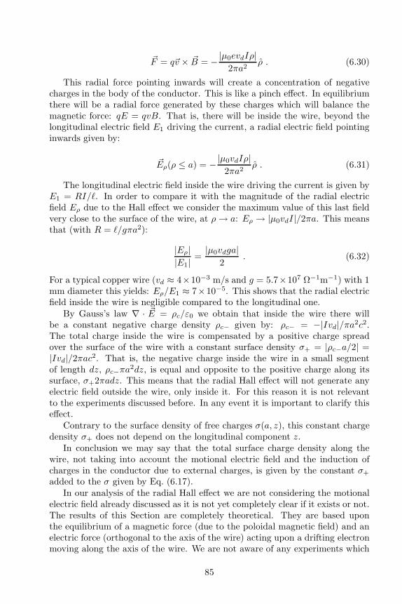
~F = q~v × ~B = −|µ0evdIρ|2πa2

ρ . (6.30)

This radial force pointing inwards will create a concentration of negativecharges in the body of the conductor. This is like a pinch effect. In equilibriumthere will be a radial force generated by these charges which will balance themagnetic force: qE = qvB. That is, there will be inside the wire, beyond thelongitudinal electric field E1 driving the current, a radial electric field pointinginwards given by:

~Eρ(ρ ≤ a) = −|µ0vdIρ|2πa2

ρ . (6.31)

The longitudinal electric field inside the wire driving the current is given byE1 = RI/ℓ. In order to compare it with the magnitude of the radial electricfield Eρ due to the Hall effect we consider the maximum value of this last fieldvery close to the surface of the wire, at ρ → a: Eρ → |µ0vdI|/2πa. This meansthat (with R = ℓ/gπa2):

|Eρ||E1|

=|µ0vdga|

2. (6.32)

For a typical copper wire (vd ≈ 4×10−3 m/s and g = 5.7×107 Ω−1m−1) with 1mm diameter this yields: Eρ/E1 ≈ 7×10−5. This shows that the radial electricfield inside the wire is negligible compared to the longitudinal one.

By Gauss’s law ∇ · ~E = ρc/ε0 we obtain that inside the wire there willbe a constant negative charge density ρc− given by: ρc− = −|Ivd|/πa2c2.The total charge inside the wire is compensated by a positive charge spreadover the surface of the wire with a constant surface density σ+ = |ρc−a/2| =|Ivd|/2πac2. That is, the negative charge inside the wire in a small segmentof length dz, ρc−πa

2dz, is equal and opposite to the positive charge along itssurface, σ+2πadz. This means that the radial Hall effect will not generate anyelectric field outside the wire, only inside it. For this reason it is not relevantto the experiments discussed before. In any event it is important to clarify thiseffect.

Contrary to the surface density of free charges σ(a, z), this constant chargedensity σ+ does not depend on the longitudinal component z.

In conclusion we may say that the total surface charge density along thewire, not taking into account the motional electric field and the induction ofcharges in the conductor due to external charges, is given by the constant σ+

added to the σ given by Eq. (6.17).In our analysis of the radial Hall effect we are not considering the motional

electric field already discussed as it is not yet completely clear if it exists or not.The results of this Section are completely theoretical. They are based uponthe equilibrium of a magnetic force (due to the poloidal magnetic field) and anelectric force (orthogonal to the axis of the wire) acting upon a drifting electronmoving along the axis of the wire. We are not aware of any experiments which

85

tried to measure the internal density of charges ρc− in current carrying metallicconductors.

We now compare all three components of the electric field outside the wirewith one another.

6.5 Discussion

The solutions presented here will remain valid in the case of a hollow cylindricalshell of internal radius ai and external radius a. The internal density of surfacecharge at ρ = ai will be zero taking into account the approximations consideredhere, while the external density of surface charge will be the same as obtainedbefore. The main difference is that the electric field in the region ρ < ai willnot produce any current as there is no conductor in this region.

Although many authors forget about the zeroth order force F0 due to elec-trostatic induction when dealing with a current-carrying wire interacting withan external charge, there is no doubt it exists. Comparing the three componentsof the force already discussed, it is the only one which diverges as we approachthe wire. If we are far away from the wire (at a distance ρ≫ a from it) this ze-roth order force falls as 1/ρ2 ln(ρ/a) (as we saw in Eqs. (4.81) and (4.83)), whilethe radial component of the force proportional to the voltage of the battery andof the second order force, F1 and F2, fall as 1/ρ (as we saw in Eqs. (6.21) and(6.27)).

We now compare the three components of this force given by Eqs. (4.81)and (4.82), (6.21) and (6.27). To this end we consider a particular examplewith orders of magnitudes similar to those employed in Sansbury’s experiment[178]. He utilized a U-shaped copper current conductor (50 cm long legs spaced10 cm apart, with 0.95 cm diameter). As we will utilize his dimensions in adifferent configuration (straight wire instead of a U-shaped conductor), we willconsider our straight wire having a total length of ℓ = 1.20 m and a radiusa = 4.75× 10−3 m. The conductivity of copper is g = 5.7× 107 Ω−1m−1 and ithas a number of free electrons per unit volume given by n = 8.5×1028 m−3. Theresistance of the wire is then given by R = ℓ/gπa2 = 3.0 × 10−4 Ω. He passeda current of 900 A in his wire, which means a potential difference between theextremities of the wire as given by φL − φR = 0.27 V. The drifting velocity inthis case amounts to vd = I/πa2en = 0.9×10−3 m/s. We will suppose moreoverthe symmetrical case in which φR = −φL = −0.135 V. The test charge will bethe one estimated by Sansbury, namely, q ≈ 5×10−10 C, at a distance of ρ = 3.5cm = 3.5 × 10−2 m from the wire. This yields a/ρ′ = 0.121. Although his testcharge was spread over a 2 cm × 2 cm silver foil, here we suppose the test chargeconcentrated in a point.

These values in Eqs. (4.81) and (4.82) yield αL = 0.247, F0 = 4.5 × 10−7

N and E0 = F0/q = 9.0 × 102 V/m. Although Sansbury observed a zerothorder force, he did not measure it. For comparison we present here the zerothorder force upon an electron (q = −1.6 × 10−19 C) and upon a typical chargegenerated by friction (q ≈ 10−6 C) at the same distance from the same wire,

86

namely: F0 = 4.6 × 10−26 N and F0 = 1.8 N, respectively. The huge differencebetween these forces arises from the fact that F0 is proportional to the squareof q. The corresponding zeroth order electric fields due to the electron andto the charge generated by friction are given by E0 = 2.9 × 10−7 V/m andE0 = 1.8 × 106 V/m, respectively.

We now consider the force F1 and electric field E1 = F1/q proportional tothe voltage of the battery. We consider only the radial component along the ρdirection given by Eq. (6.21). This component depends upon the values of thepotentials at the extremities of the wire and also upon the value of z. With thegiven symmetrical potentials, φL + φR = 0 V, then the radial components ofF1 and of E1 go to zero at z = 0. The maximal magnitudes of F1 and of E1

happen at z = ±ℓ/2. At these locations, with q = 5 × 10−10 C and with thegiven conditions we obtain: F1 = 3.5 × 10−10 N and E1 = 0.69 V/m.

As regards the second order effect, we utilize Eq. (6.27). With q = 5×10−10

C and the given conditions we obtain: F2 = 1.2 × 10−15 N. This yields E2 =F2/q = 2.4 × 10−6 V/m.

Finally we can compare the three force components along the radial direction(for F1 we consider only the maximal value). Utilizing q = 5 × 10−10 C weobtained: F0 = 4.5× 10−7 N, F1 = 3.5× 10−10 N and F2 = 1.2× 10−15 N. Thecorresponding components of the electric field were given by: E0 = 9.0 × 102

V/m, E1 = 6.9 × 10−1 V/m and E2 = 2.4 × 10−6 V/m. This yields F0/F1 =1.3× 103, F1/F2 = 2.9 × 105, E0/E1 = 1.3× 103 and E1/E2 = 2.9 × 105. Thatis, in this case F0 ≫ F1 ≫ F2 and E0 ≫ E1 ≫ E2.

Similar order of magnitudes are obtained in the experiment of Bartlett andMaglic [179].

To facilitate the detection of the force F1 it would be better not to placeany test charge close to the wire. Instead of this, it would be ideal to bring asmall neutral conductor close to the wire. In principle it would not act uponthe wire. But when we pass a current upon the resistive wire, this wire shouldbecome charged along its surface. Therefore, it should generate an electric fieldE1 outside it. This electric field would then polarize the small conductor outsideit. Consequently, there would arise an attraction between the conductor andthe current-carrying wire. We have already seen experiments of this kind inChapter 3.

The second possibility in order to facilitate the detection of the force F1 evenin the presence of the force F0 (in the case in which we approach a charged bodyto the current-carrying wire) would be to increase the voltage of the batteryconnected to the wire. As F1 is proportional to the emf of the battery, we canmake F1 greater than F0 working with high resistance wires connected to highvoltages. We also saw experiments of this kind in Chapter 3.

In many cases we will have F0 ≫ F1 ≫ F2. Despite this fact the force~F1 has already been observed in the laboratory, as we saw in Chapter 3. Weconsider the current flowing in the top part of a circuit like that of our Figure 6.1,with symmetrical potentials: φR = −φL. In order to compare these theoreticalresults with the experiments, we need to obtain the lines of electric field. Toobtain these lines we follow the approach presented in Sommerfeld’s book [208,

87

pp. 125-130] (German original from 1948 based on lectures delivered in 1933-1934). We obtain this in the plane xz (y = 0). Any plane containing thez axis will yield a similar solution. The lines of electric field are orthogonaltrajectories to the equipotential lines. As ~E = −∇φ, the electric field pointsalong the direction of the maximum space rate of change of φ. We are thenlooking for a function ξ(ρ, z) such that

∇ξ(ρ, z) · ∇φ(ρ, z) = 0 . (6.33)

For ρ < a we have φ as a linear function of z, such that ξ can be foundproportional to ρ. We write it as ξ(ρ < a, z) = −Aℓρ, with A as a constant.The equipotential lines, φ(ρ, z) = constant, can be written as z1(ρ) = K1,where K1 is a constant (for each constant we have a different equipotentialline). Analogously, the lines of electric field will be given by z2(ρ) = K2, whereK2 is another constant (for each K2 we have a different line of electric field).From Eq. (6.33) we get dz2/dρ = −1/(dz1/dρ) = (∂φ/∂z)/(∂φ/∂ρ). Integratingthis equation we can obtain ξ(ρ, z). With Eq. (6.9) this yields the solution forρ > a. We are then led to:

ξ(ρ, z) = (φR − φL)ρ

ℓif ρ < a , (6.34)

ξ(ρ, z) = (φR + φL)z

ℓ+ (φR − φL)

(

ρ2

2ℓ2+z2

ℓ2− ρ2

ℓ2lnρ

ℓ

)

if ρ > a . (6.35)

From these equations we can easily verify Eq. (6.33).In order to compare these results with the experiments of Bergmann, Schae-

fer, Jefimenko, Barnett and Kelly we need essentially the value of ℓ/a. FromFigure 3.1 we get ℓ/a ≈ 33, from Figure 3.3 we get ℓ/a ≈ 13, while from Fig-ure 3.10 we get ℓ/a ≈ 4. The plots of the equipotentials between z = −ℓ/2and ℓ/2 given by Eqs. (6.8) and (6.9) with these values of ℓ/a are given inFigures 6.3, 6.4 and 6.5 (with the experimental results of Bergmann, Schaefer,Jefimenko, Barnett and Kelly overlaid on them).

Plots of the lines of electric field given by Eqs. (6.34) and (6.35) with thesevalues of ℓ/a are given in Figures 6.6, 6.7 and 6.8 (with the experimental resultsof Bergmann, Schaefer, Jefimenko, Barnett and Kelly overlaid on them).

These theoretical Figures overlaid on the experimental ones indicate a verygood agreement between theory and experiment.

We now consider Sansbury’s experiment discussed in Chapter 3. The ob-served force was of the order of 10−7 N, although he was not able to make precisemeasurements. He analyzed briefly the possibility that this extra force might bethe force F1 discussed here, but only considered the longitudinal electric fieldoutside the wire. He then concluded that this force would be three orders ofmagnitude smaller than the effect he measured. However, he was not aware ofthe radial component of ~E1, which can be larger than the longitudinal compo-nent, as we showed here. Moreover, his U-shaped wire was bent close to the foil

88

Figure 6.3: Theoretical equipotential lines overlaid on the experimental lines ofelectric field obtained by Bergmann and Schaefer.

Figure 6.4: Theoretical equipotential lines overlaid on the experimental lines ofelectric field obtained by Jefimenko.

and thus the approximation to a long straight wire may not be applicable. Closeto a corner the electric field outside the wire is even larger than the longitudinalone inside it [167]. Possibly what Sansbury detected directly was the force F1

discussed here. It would be important to repeat his experiment carefully takingthis into account.

In this Chapter we have seen a first example in which the electric field insideand outside a resistive wire carrying a steady current is due to charges spreadalong the surface of the conductor. The density of these surface charges is con-stant in time but varies along the length of the wire. It is proportional to thevoltage generated by the battery connected to the wire. As the internal and ex-ternal electric field is produced by charges at the surface of the wire, we can seea direct connection between electrostatics (represented by Gauss’s law) and cir-cuit theory (represented by Ohm’s law). This allows a connection between these

89

Figure 6.5: Theoretical equipotential lines overlaid on the experimental onesobtained by Jefimenko, Barnett and Kelly.

Figure 6.6: Theoretical lines of electric field overlaid on the experimental onesobtained by Bergmann and Schaefer.

two topics which are usually considered separately in the textbooks. Despitethis fact some authors have called attention to the strong connection betweenthese two branches of electromagnetism, beginning with Weber and Kirchhoff,as we see in the Appendices. Some modern scientists mention the same aspect[209, 210, 211, 171] [166, Chapter 18: A Microscopic View of Electric Circuits,pp. 623-666].

The example discussed here is important to show clearly the existence ofan external electric field proportional to the potential difference acting uponthe resistive wire, even in the case of a straight wire carrying a steady current.This electric field does not depend upon a variable current (with a longitudinalacceleration of the electrons along the direction of the wire), nor of a centripetalacceleration of the conduction electrons (due to any curvature in the wire). Thatis, this external electric field will exist even when there is no acceleration of the

90

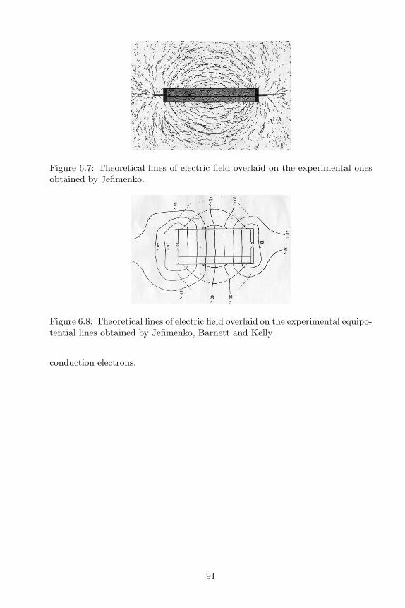
Figure 6.7: Theoretical lines of electric field overlaid on the experimental onesobtained by Jefimenko.

Figure 6.8: Theoretical lines of electric field overlaid on the experimental equipo-tential lines obtained by Jefimenko, Barnett and Kelly.

conduction electrons.

91

92

Chapter 7

Coaxial Cable

7.1 Introduction

Many authors studied the distribution of surface charges in resistive coaxialcables carrying steady currents, as well as the potential and electric field insideand outside the conductors [212, pp. 175-184] [170] [208, pp. 125-130] [213][214] [176, pp. 318 and 509-511] [12] [215] [16, pp. 336-337] [216] [217].

Here we present the main results in this configuration considering the generalcase of a return conductor of finite area and finite conductivity. In this casethere will be an electric field outside the external return conductor, althoughthe magnetic field goes to zero in this region.

The configuration of the problem is that of Figure 7.1.

Figure 7.1: Configuration of the problem.

A constant current I flows uniformly in the z direction along the innerconductor (radius a and conductivity g1), returning uniformly along the outerconductor (internal and external radii b and c, respectively, and conductivity g3).The conductors have uniform circular cross-sections and a length ℓ≫ c > b > acentered on z = 0. The medium outside the conductors is considered to be airor vacuum. The potentials at the extremities located at z = ℓ/2 of the inner andouter conductors are maintained at the constant values φA and φB, respectively.The potentials at the extremities located at z = −ℓ/2 of the outer and inner

93

conductors are maintained at the constant values φC and φD, respectively.

7.2 Potentials and Fields

We are interested in calculating the potentials and fields in a point ~r = (ρ, ϕ, z)such that ℓ ≫ ρ and ℓ ≫ |z|, so that we can neglect edge effects. All solutionspresented here were obtained with this approximation. With this approximationand configuration we then have the potential as a linear function of z. SeeSection 5.4. In order to have uniform currents flowing in the z direction alongthe inner and outer conductors, with a potential satisfying the given values atthe extremities, we have:

φ(ρ ≤ a, ϕ, z) =φA + φD

2+ (φA − φD)

z

ℓ, (7.1)

φ(b ≤ ρ ≤ c, ϕ, z) =φC + φB

2+ (φB − φC)

z

ℓ. (7.2)

By Ohm’s law (with R1 and R3 being the resistances of the inner and outerconductors, respectively) we obtain:

φD − φA = R1I =ℓI

πg1a2, (7.3)

φB − φC = R3I =ℓI

πg3(c2 − b2). (7.4)

In the four regions (ρ < a, a < ρ < b, b < ρ < c and c < ρ) the potential φsatisfies Laplace’s equation ∇2φ = 0. By Eqs. (7.1) and (7.2) we have the valueof φ in the first and third regions, which also supply the boundary conditionsat ρ = a and at ρ = b in order to find φ in the second region. To find φ in thefourth region we need another boundary condition, in addition to the value ofφ at ρ = c, which is given by Eq. (7.2). We then impose the following boundarycondition:

φ(ρ = ℓ, ϕ, z) = 0 V . (7.5)

This is the main non-trivial boundary condition for this problem. The samereasoning was utilized in Section 6.2 after Eq. (6.21). This equation says that thepotential goes to zero at a radial distance ρ = ℓ, so that the length ℓ of the cableappears in the solution. The usual condition φ(ρ → ∞, ϕ, z) = 0 V does notwork in the situation considered here. We first tried this last condition but couldnot obtain a correct solution for the potential, and only discovered Eq. (7.5)working backwards. That is, from the work of Russell we knew that in generalthe density of the surface charges on a system of long parallel homogeneousconductors in steady-state (as is the case of the coaxial cable being consideredhere) varies linearly with distance along the direction of their common axis [9].That is, if d represents a, b or c, the surface charge densities at these surfaces

94

must be given by σd(z) = Ad+Bdz, with the constants Ad and Bd characterizingeach surface. We then obtained the potential at all points in space by

φ(~r) =1

4πε0

3∑

j=1

∫ ∫

Sj

σ(~rj)daj|~r − ~rj |

. (7.6)

Here the sum goes over the three surfaces ρ = a, b and c, extending fromz = −ℓ/2 to z = ℓ/2. After solving these integrals we discovered that φ wentto zero not at infinity, but at ρ = ℓ. Although this difference is importantmathematically in order to arrive at a working solution, physically we can saythat the potential going to zero at ρ = ℓ is equivalent to it going to zero atinfinity. As we suppose ℓ ≫ c > b > a, we are essentially imposing that thepotential goes to zero at a large distance from the cable, which is reasonable.

Here we reverse the argument, as this is more straightforward. That is, webegin with the boundary conditions for φ, obtaining the solutions of Laplace’sequation, the electric field ~E = −∇φ and then σ by Gauss’s law.

The boundary conditions are then the values of φ at ρ = a, ρ = b, ρ = c andρ = ℓ. They are given by Eqs. (7.1), (7.2) and (7.5). The solutions of Laplace’sequation ∇2φ = 0 for a ≤ ρ ≤ b and for c ≤ ρ in cylindrical coordinatessatisfying these boundary conditions yield:

φ(a ≤ ρ ≤ b, ϕ, z) =φB + φC

2+ (φB − φC)

z

ℓ

+

[

φA + φD − φC − φB2

+ (φA − φD + φC − φB)z

ℓ

]

ln(b/ρ)

ln(b/a), (7.7)

φ(c ≤ ρ, ϕ, z) =

[

φC + φB2

+ (φB − φC)z

ℓ

]

ln(ℓ/ρ)

ln(ℓ/c). (7.8)

The lines of electric field are given by a function ξ(ρ, z) such that ∇ξ·∇φ = 0.By the procedure described in the previous Chapter we obtain

ξ(ρ < a, ϕ, z) = −(φA − φD)ρ

ℓ, (7.9)

ξ(a < ρ < b, ϕ, z) =φA + φD − φC − φB

2

z

ℓ+φB − φC

2

ρ2

ℓ2lnb

a

+φA − φD + φC − φB

2

(

z2

ℓ2+

ρ2

2ℓ2− ρ2

ℓ2lnρ

b

)

, (7.10)

ξ(b < ρ < c, ϕ, z) = −(φB − φC)ρ

ℓ, (7.11)

ξ(c < ρ, ϕ, z) =φB + φC

2

z

ℓ+φB − φC

2

(

z2

ℓ2+

ρ2

2ℓ2− ρ2

ℓ2lnρ

ℓ

)

. (7.12)

95

The electric field ~E = −∇φ is given by

~E(ρ < a, ϕ, z) =φD − φA

ℓz , (7.13)

~E(a < ρ < b, ϕ, z) =

[

φA + φD − φC − φB2

+ (φA − φD + φC − φB)z

ℓ

] 1

ln(b/a)

ρ

ρ

+

[

φC − φBℓ

+φD − φA + φB − φC

ℓ

ln(b/ρ)

ln(b/a)

]

z , (7.14)

~E(b < ρ < c, ϕ, z) =φC − φB

ℓz , (7.15)

~E(c < ρ, ϕ, z) =

[

φC + φB2

+ (φB − φC)z

ℓ

]

1

ln(ℓ/c)

ρ

ρ

+φC − φB

ℓ

ln(ℓ/ρ)

ln(ℓ/c)z . (7.16)

The main points to be emphasized here are the solutions (7.8) and (7.16).They show the existence of an electric field outside the resistive cable even whenit is carrying a constant current.

Here we do not consider the motional electric field proportional to secondorder in vd/c. Its order of magnitude is much smaller than the one consideredhere (proportional to the potential difference along the cable). For this reasonwe do not need to take it into account here.

The surface charge densities σ along the inner conductor (ρ = a, σa(z)) andalong the inner and outer surfaces of the return conductor (ρ = b, σb(z) andρ = c, σc(z)) can be obtained easily utilizing Gauss’s law:

∫

©∫

S

~E · d~a =Q

ε0, (7.17)

where d~a is the surface element pointing normally outwards the closed surfaceS and Q is the net charge inside S. This yields σa(z) = ε0E2ρ(ρ → a, z),σb(z) = −ε0E2ρ(ρ → b, z) and σc(z) = ε0E4ρ(ρ → c, z), where the subscripts

2ρ and 4ρ mean the radial component of ~E in the second and fourth regions,a < ρ < b and c < ρ, respectively. This means that:

σa(z) =ε0a

1

ln(b/a)

[

φA + φD − φC − φB2

+ (φA − φD + φC − φB)z

ℓ

]

, (7.18)

96

σb(z) = −abσa(z) , (7.19)

σc(z) =ε0c

1

ln(ℓ/c)

[

φC + φB2

+ (φB − φC)z

ℓ

]

. (7.20)

An alternative way of obtaining φ and ~E is to begin with the surface chargesas given by Eqs. (7.18) to (7.20). We then calculate the electric potential φ (and~E = −∇φ) through Eq. (7.6). We checked the calculations with this procedure.

7.3 The Symmetrical Case

In order to visualize the equipotentials and lines of electric field we considerℓ/c = 5, ℓ/b = 15/2 and ℓ/a = 15. There are two main cases of interest, thesymmetrical and asymmetrical cases. In the symmetrical case there are twoequal batteries located at both extremities of the cable, Figure 7.2.

Figure 7.2: The symmetrical case.

They generate potentials φB = φD = −φA = −φC ≡ φ0/2. In this case thesurface charge densities go to zero at the center of the cable (z = 0) in all threesurfaces (ρ = a, b and c). The equipotentials and lines of electric field for thissituation are shown in Figures 7.3 and 7.4, respectively.

Figure 7.3: Equipotential lines for the symmetrical case.

97

Figure 7.4: Lines of electric field for the symmetrical case.

In this case the potential is simply proportional to z without any additiveconstant. We can then write it in terms of the currents and conductivities asgiven by:

φ(ρ ≤ a) = − Iz

πg1a2, (7.21)

φ(a ≤ ρ ≤ b) = − I

π

z

ln(b/a)

[

ln(b/ρ)

g1a2− ln(ρ/a)

g3(c2 − b2)

]

, (7.22)

φ(b ≤ ρ ≤ c) =Iz

πg3(c2 − b2), (7.23)

φ(c ≤ ρ) =I

π

ln(ℓ/ρ)

ln(ℓ/c)

z

g3(c2 − b2). (7.24)

Particular cases include an equipotential outer conductor (φC = φB = 0)with an infinite area (c → ∞) or with an infinite conductivity (g3 → ∞).These solutions are recovered taking g3(c

2 − b2) → ∞, such that σc(z) → 0,~E(ρ > b) → 0 and φ(ρ ≥ b) → 0 for any z. The opposite solution when thecurrent flows in an inner conductor of infinite conductivity, returning in an outerconductor of finite area and finite conductivity, is also easily obtained from theprevious result, yielding ~E(ρ < a) → 0 and φ(ρ ≤ a) → 0 for any z.

7.4 The Asymmetrical Case

In the asymmetrical case there is a battery at the left extremity and a loadresistance RL at the right extremity, Figure 7.5.

We can represent the potentials generated by the battery producing a voltageφ0 between its terminals as φD = −φC ≡ φ0/2. By Ohm’s law the total current

98

Figure 7.5: The asymmetrical case.

I is related to the total resistanceRt ≡ R1+RL+R2 by I = φ0/Rt. Analogously:φD−φA = φ0(R1/Rt), φA−φB = φ0(RL/Rt) and φB−φC = φ0(R2/Rt). Theseresults in Eqs. (7.1) to (7.12) yield:

φ(ρ ≤ a, ϕ, z) = φ0

(

R2 +RL2Rt

− R1

Rt

z

ℓ

)

, (7.25)

φ(a ≤ ρ ≤ b, ϕ, z) = −φ0

[(

R1 +RL2Rt

− R1 +R2 + 2RL2Rt

ln(b/ρ)

ln(b/a)

)

−(

R2

Rt− R1 +R2

Rt

ln(b/ρ)

ln(b/a)

)

z

ℓ

]

, (7.26)

φ(b ≤ ρ ≤ c, ϕ, z) = −φ0

(

R1 +RL2Rt

− R2

Rt

z

ℓ

)

, (7.27)

φ(c ≤ ρ, ϕ, z) = −φ0

(

R1 +RL2Rt

− R2

Rt

z

ℓ

)

ln(ℓ/ρ)

ln(ℓ/c). (7.28)

ξ(ρ < a, ϕ, z) = φ0R1

Rt

ρ

ℓ, (7.29)

ξ(a < ρ < b, ϕ, z) = φ0

[

R1 +R2 + 2RL2Rt

z

ℓ+

R2

2Rt

ρ2

ℓ2lnb

a

− 1

2

(

z2

ℓ2+

ρ2

2ℓ2− ρ2

ℓ2lnρ

b

)]

, (7.30)

ξ(b < ρ < c, ϕ, z) = −φ0R2

Rt

ρ

ℓ, (7.31)

ξ(c < ρ, ϕ, z) = −φ0

[

R1 +RL2Rt

z

ℓ− R2

2Rt

(

z2

ℓ2+

ρ2

2ℓ2− ρ2

ℓ2lnρ

ℓ

)]

. (7.32)

These Equations are plotted in Figures 7.6 and 7.7 when ℓ/c = 5, ℓ/b = 15/2,ℓ/a = 15 and R1 = R2 = RL.

As we obtained algebraic solutions for the fields, potentials and surfacecharges, it is easy to apply them for commercial cables. In this way we canknow the orders of magnitude of these quantities for several standard cables.

99

Figure 7.6: Equipotential lines for the asymmetrical case.

Figure 7.7: Lines of electric field for the asymmetrical case.

7.5 Discussion

The distribution of charges given by Eqs. (7.18) to (7.20) is equivalent to equaland opposite charges in the facing surfaces. That is, the charge at the positionρ = a, z, in a length dz, dqa(z) = 2πaσa(z)dz, is equal and opposite to the chargeat the position ρ = b, z, in the same length dz: dqb(z) = 2πbσb(z)dz = −dqa(z).

The electric field outside the coaxial cable then depends only on the surfacecharges at the external wall of the return conductor, σc(z):

φ(c ≤ ρ, ϕ, z) =c

ε0σc(z) ln

ℓ

ρ=

[

φB + φC2

+ (φB − φC)z

ℓ

]

ln(ρ/ℓ)

ln(c/ℓ). (7.33)

The main nontrivial conclusions of this analysis are Eqs. (7.16) and (7.33).They show that although there is no vector potential or magnetic field outside

100

a coaxial cable, the electric field will be different from zero when there is a finiteresistivity in the outer conductor. To our knowledge the first to mention thisexternal electric field outside a resistive coaxial cable was Russell in his impor-tant paper of 1983 [213]. The solution of this Chapter presents an analyticalcalculation of this field.

This external electric field indicates that there is no shielding in a coaxialcable with a resistive outer conductor (sheath). It is important to realize thisspecially when dealing with interferences in telecommunication systems. Evenwith a long cable there will be this external electric field, as can be seen fromEq. (7.33). For this reason this resistive cable will influence other electricalsystems nearby. This field will be present even for variable current. This is arelevant aspect neglected by most authors.

101

102

Chapter 8

Transmission Line

8.1 Introduction

One of the most important electrical systems is that of a two-wire transmissionline, usually called twin-leads. We consider here homogeneous resistive wiresfixed in the laboratory and carrying steady currents. The goal here is to calculatethe electric field outside the wires.

The case of twin-leads was first considered by Stratton [218, p. 262]. Al-though he called attention to the electric field outside the transmission line, thishas been forgotten by most authors, as we have seen. We treated this case inmore detail in 1999 [219] and here we follow this latter approach. These are theonly theoretical works dealing with this configuration known to us.

8.2 Two-Wire Transmission Line

The configuration of the system is given in Figure 8.1.We have two equal straight wires of circular cross-sections of radii a and

length ℓ, surrounded by air. Their axes are separated by a distance b and areparallel to the z axis, symmetrically located relative to the z and x axes. That is,the centers of the wires are located at (x, y, z) = (−b/2, 0, 0) and (+b/2, 0, 0).The conductivity of the wires is g and their extremities are located at z = −ℓ/2and z = +ℓ/2. Here we calculate the electric potential φ and the electric field~E at a point (x, y, z) such that ℓ ≫ r =

√

x2 + y2 + z2. Moreover, we alsoassume that ℓ≫ b/2 > a, so that we can neglect edge effects.

We want to find the potential and electric field when a current I flows uni-formly through one of the wires along the direction +z and returns uniformlythrough the other wire along the direction −z. The current densities in bothwires are then given by ~J = (I/πa2)z and ~J = −(I/πa2)z, respectively. As weare considering homogeneous wires with a constant conductivity g, Ohm’s lawyields the internal electric field in the wires as ~E = ±(I/gπa2)z. We do not

need to consider in ~E the influence of the time variation of the vector potential

103

Figure 8.1: Two homogeneously resistive parallel wires of radii a separated by adistance b. The first wire carries a steady current I along the positive z directionwhile the second wire carries the return current I along the negative z direction.

as we are dealing with a steady current in stationary wires, so that ∂ ~A/∂t = ~0

everywhere. We can then write ~E = −∇φ. As we have a constant electric fieldin each wire, this implies that the potential is constant over each cross-sectionand a linear function of z. In this work we consider a symmetrical situation forthe potentials so that in the first wire the current flows from the potential φL atz = −ℓ/2 to φR at z = ℓ/2 and returns in the second wire from −φR at z = ℓ/2to −φL at z = −ℓ/2, Figure 8.1. We can then write:

φF (z) =φR + φL

2+ (φR − φL)

z

ℓ=φR + φL

2+

I

gπa2z , (8.1)

φS(z) = −φF (z) . (8.2)

In these equations φF (z) and φS(z) are the potentials as a function of z overthe cross-section of the first and second conductors, respectively.

In this Chapter we neglect the small Hall effect due to the azimuthal mag-netic field generated by these currents. See Section 6.4. This effect creates aredistribution of the charge density within the wires, and modifies the surfacecharges also. As these are usually small effects, they will not be considered here.

We now find the potential in space supposing there is air outside the conduc-tors. As the conductors are straight and the boundary conditions (the potentialsover the surface of the conductors) are linear functions of z, the same must bevalid everywhere, as we saw in Section 5.4. That is, φ = (A+Bz)f(x, y), whereA and B are constants and f(x, y) is a function of x and y. This function canbe found by the method of images, imposing a constant potential φ0 over thefirst wire and −φ0 over the second one [13, Section 2.1]. The final solution for

φ and ~E satisfying the given boundary conditions, valid for the region outsidethe wires, is given by:

104

φ(x, y, z) = −(

φR + φL2

+ (φR − φL)z

ℓ

)

1

2 ln b−√b2−4a2

2a

× ln(x−

√b2 − 4a2/2)2 + y2

(x+√b2 − 4a2/2)2 + y2

, (8.3)

~E = −(

φR + φL2

+ (φR − φL)z

ℓ

)√b2 − 4a2

ln b+√b2−4a2

2a

× (x2 − y2 + a2 − b2/4)x+ 2xyy

D41

+φR − φL

ℓ

1

2 ln b−√b2−4a2

2a

[

ln(x −

√b2 − 4a2/2)2 + y2

(x +√b2 − 4a2/2)2 + y2

]

z , (8.4)

where:

D41 ≡ x4 + y4 + b4/16 + a4 + 2x2y2 − b2x2/2

+ 2a2x2 + b2y2/2 − 2a2y2 − b2a2/2 . (8.5)

The equipotentials at z = 0 are plotted in Figure 8.2.

Figure 8.2: Equipotentials in the plane z = 0.

It is also relevant to express these results in cylindrical coordinates (ρ, ϕ, z)centered on the first and second wires. See Figure 8.3.

105

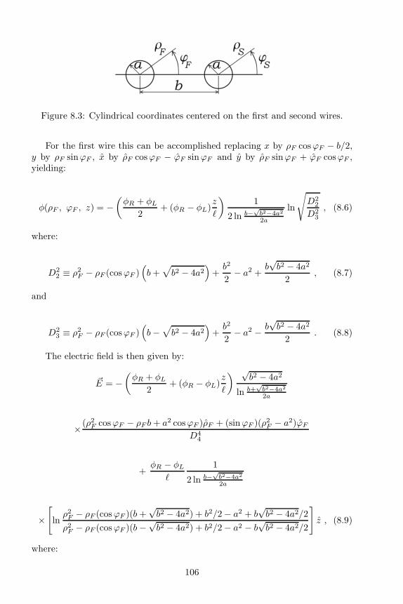
Figure 8.3: Cylindrical coordinates centered on the first and second wires.

For the first wire this can be accomplished replacing x by ρF cosϕF − b/2,y by ρF sinϕF , x by ρF cosϕF − ϕF sinϕF and y by ρF sinϕF + ϕF cosϕF ,yielding:

φ(ρF , ϕF , z) = −(

φR + φL2

+ (φR − φL)z

ℓ

)

1

2 ln b−√b2−4a2

2a

ln

√

D22

D23

, (8.6)

where:

D22 ≡ ρ2

F − ρF (cosϕF )(

b+√

b2 − 4a2)

+b2

2− a2 +

b√b2 − 4a2

2, (8.7)

and

D23 ≡ ρ2

F − ρF (cosϕF )(

b−√

b2 − 4a2)

+b2

2− a2 − b

√b2 − 4a2

2. (8.8)

The electric field is then given by:

~E = −(

φR + φL2

+ (φR − φL)z

ℓ

)√b2 − 4a2

ln b+√b2−4a2

2a

× (ρ2F cosϕF − ρF b+ a2 cosϕF )ρF + (sinϕF )(ρ2

F − a2)ϕFD4

4

+φR − φL

ℓ

1

2 ln b−√b2−4a2

2a

×[

lnρ2F − ρF (cosϕF )(b +

√b2 − 4a2) + b2/2 − a2 + b

√b2 − 4a2/2

ρ2F − ρF (cosϕF )(b −

√b2 − 4a2) + b2/2 − a2 − b

√b2 − 4a2/2

]

z , (8.9)

where:

106

D44 ≡ ρ4

F − 2ρ3F b cosϕF + ρ2

F b2 + a4

+ 2ρ2Fa

2(cos2 ϕF − sin2 ϕF ) − 2ρF ba2 cosϕF . (8.10)

The density of surface charges over the first and second wires, σF and σS ,can then be found by ε0 times the radial component of the electric field overthe surface of each cylinder, yielding:

σF =

(

φR + φL2

+ (φR − φL)z

ℓ

)

ε0

2a ln b+√b2−4a2

2a

√b2 − 4a2

b/2 − a cosϕF, (8.11)

σS = −(

φR + φL2

+ (φR − φL)z

ℓ

)

ε0

2a ln b+√b2−4a2

2a

√b2 − 4a2

b/2 + a cosϕS. (8.12)

In order to check these results we calculated the potential φ inside each wireand in space, beginning with these surface charge densities and utilizing:

φ(x, y, z) =1

4πε0

[

∫ ℓ/2

z′=−ℓ/2

∫ 2π

ϕ′

F=0

σF (ϕ′F )adϕ′

Fdz′

|~r − ~r ′|

+

∫ ℓ/2

z′=−ℓ/2

∫ 2π

ϕ′

S=0

σS(ϕ′S)adϕ′

Sdz′

|~r − ~r ′|

]

. (8.13)

Here we integrate over the surfaces of the first and second cylinders, SL andSR, respectively. We can then check these results assuming the correctness of themethod of images for the electrostatic problem and utilizing the approximationsℓ≫ |~r| and ℓ≫ b/2 > a.

With b≫ a and b≫ ρF , Eqs. (8.11) and (8.6) yield:

σF ≈ ε0a ln(b/a)

(

φR + φL2

+ (φR − φL)z

ℓ

)

, (8.14)

and

φ(a < ρF ≪ b, ϕF , z) ≈aσF (z)

ε0ln

b

ρF. (8.15)

These results are analogous to Eqs. (6.2) and (6.9).

107

8.3 Discussion

The first aspect to be discussed here is the qualitative interpretation of theseresults. In all this Section we will assume φR = 0 in order to simplify theanalysis. The distribution of surface charges for a given z is similar to thedistribution of charges in the electrostatic problem given the potentials φ0 and−φ0 at the first and second wires, without current. That is, σF (ϕF ) > 0 for anyϕF and its maximum value is at ϕF = 0 rad. The density of surface chargesat the second wire, σS , has the same behaviour of σF with an overall change ofsign, with its maximum magnitude occurring at ϕS = π rad. A qualitative plotof the surface charges at z = 0 is given in Figure 8.4.

Figure 8.4: Qualitative distribution of surface charges for two parallel wires inthe plane z = 0.

A quantitative plot of σF is given in Figure 8.5 supposing b/2a = 10/3 andnormalizing the surface charge density by the value of σF at ϕF = π rad.

Figure 8.5: Quantitative normalized distribution of the density of surfacecharges in the first wire in the plane z = 0 as a function of the azimuthalangle.

It should also be remarked that for a fixed ϕF the surface density decreaseslinearly from z = −ℓ/2 to z = ℓ/2, the opposite happening with σS for a fixedϕS .

We can integrate the surface charges over the circumference of each wire,obtaining the integrated charge per unit length λ(z) as:

108

λF (z) =

∫ 2π

ϕF =0

aσF (ϕF )dϕF

= − 2πε0

ln [(b−√b2 − 4a2)/2a]

[

φR + φL2

+ (φR − φL)z

ℓ

]

. (8.16)

λS(z) = −∫ 2π

ϕS=0

aσS(ϕS)dϕS = −λF (z) . (8.17)

One important aspect to discuss is the experimental relevance of these sur-face charges in terms of forces. That is, as the wires have a net charge in eachsection, there will be an electrostatic force acting on them. We can then com-pare this force with the magnetic force. The latter is given essentially by (forceper unit length):

dFMdz

=µ0I

2

2πb, (8.18)

where we are supposing b/2 ≫ a.We now calculate the electric force per unit length on the first wire, integrat-

ing the force over its circumference. We consider a typical region in the middleof the wire, around z = 0, and once more suppose b/2 ≫ a:

d~FEdz

=

∫ 2π

ϕF =0

aσF (ϕF ) ~E(ρF = a, ϕF , z = 0)dϕF ≈ πε0φ2L

ln2 b/a

(

x

b+z

ℓ

)

. (8.19)

From Eqs. (8.18) and (8.19) the ratio of the magnetic to the radial elec-tric force is given by (with Ohm’s law φ2

L/I2 = R2 = (ℓ/gπa2)2, R being the

resistance of each wire):

FMFE

≈ µ0/ε02R2

ln2 b

a. (8.20)

As µ0/ε0 = 1.4 × 105 Ω2 this ratio will be usually many orders of magnitudegreater than 1. This would be of the order of 1 when R ≈ 370 Ω (supposingln(b/a) ≈ 1). This is a very large resistance for homogeneous wires.

In order to compare this force with the magnetic force we suppose typicalcopper wires of conductivities g = 5.7×107 m−1Ω−1, lengths ℓ = 1 m, separatedby a distance b = 6 mm and diameters 2a = 1 mm. This means that by Ohm’slaw φ2

L/I2 = R2 ≈ 5× 10−4 Ω2. With these values the ratio of the longitudinal

electric force to the magnetic force is of the order of 7×10−11, while the ratio ofthe radial electric force to the magnetic force is of the order of 1 × 10−8. Thatis, the electric force between the wires due to these surface charges is typically10−8 times smaller than the magnetic force. This shows that we can usuallyneglect these electric forces.

109

Despite this fact it should be remarked that while the magnetic force is re-pulsive in this situation (parallel wires carrying currents in opposite directions),the radial electric force is attractive, as we can see from the charges in Figure 8.4.

The situation described in this Chapter is very similar to the experimentsperformed by Bergmann, Schaefer and Jefimenko, whose results are presentedin Figures 3.2 and 3.5. We can compare these experiments with the theoreticalcalculations by plotting the equipotentials obtained here. We need essentiallythe values of ℓ/b, b/2a and ℓ/2a. From Fig. 3.2 we obtain ℓ/b ≈ 2.8, b/2a ≈ 7.4and ℓ/2a ≈ 20.7. From Fig. 3.5 we have ℓ/b ≈ 1.9, b/2a ≈ 3.0 and ℓ/2a ≈ 5.7.These values together with φA = 0 V and φB = 1 V yielded the equipotentialsgiven by Eq. (8.3) at y = 0, Figures 8.6 and 8.7.

Figure 8.6: Theoretical equipotential lines overlaid on the experimental lines ofelectric field obtained by Bergmann and Schaefer.

The lines of electric field orthogonal to the equipotentials can be obtained bythe procedure described in Sommerfeld’s book, discussed in Section 6.5. Thisyields the following solutions in the plane y = 0 outside the wires:

ξout(x, 0, z) = −(φR + φL)z

ℓ+ (φR − φL)

[

x(x2 − 3x2o)

6xoℓ2ln

(x− xo)2

(x+ xo)2

+x2o

3ℓ2ln

(x− xo)2(x+ xo)

2

x4o

− x2

3ℓ2− z2

ℓ2

]

, (8.21)

where xo ≡√b2 − 4a2/2.

The lines of electric field inside the first and second wires can be written as,respectively:

ξF (x, 0, z) = −(φR − φL)|x+ b/2|

ℓ, (8.22)

110

Figure 8.7: Theoretical equipotential lines overlaid on the experimental lines ofelectric field obtained by Jefimenko.

ξS(x, 0, z) = (φR − φL)|x− b/2|

ℓ. (8.23)

With the previous values of ℓ/b, b/2a and ℓ/2a for the two experimentsalready mentioned we obtain the lines of electric field by these equations asgiven in Figures 8.8 and 8.9 (with Figure 3.2 and the left side of Figure 3.5overlaid on them).

Figure 8.8: Theoretical lines of electric field overlaid on the experimental linesobtained by Bergmann and Schaefer.

These numerical plots are very similar to the experiments, especially in theregion between the wires. Although this calculation is strictly valid only forr ≪ ℓ, the numerical plots go from z = −ℓ/2 to ℓ/2. As the result is in rea-

111

Figure 8.9: Theoretical lines of electric field overlaid on the experimental linesobtained by Jefimenko.

sonable agreement with the experiments, we conclude that the exact boundaryconditions at z = ±ℓ/2 are not very relevant in these particular configurations.

We can also estimate the ratio of the radial component of the electric fieldto the axial component just outside the wire. We consider the first wire at threedifferent values of z: z = −ℓ/2, z = 0 and z = ℓ/2. The axial component Ez isconstant over the cross-section and does not depend on z. On the other hand,the radial component Ex is a linear function of z and also depends on ϕF . Inthis comparison we consider ϕF = 0. With these values and Jefimenko’s data inEq. (8.4) we obtain Ex/Ez ≈ 12 at z = −ℓ/2, 6 at z = 0 and 0 at z = ℓ/2. Thatis, the radial component of the electric field just outside the wire is typicallyone order of magnitude larger than the axial electric field responsible for thecurrent. Jefimenko’s experiment gives a clear confirmation of this fact.

112

Chapter 9

Resistive Plates

9.1 Introduction

In this Chapter we consider one or more resistive plates carrying steady currents.We consider an ideal case of an infinite resistive bidimensional plate (like aninfinite plane). The current is supposed to flow uniformly over the plate alonga straight direction.

When there is no current flowing in the conducting plate and we approximatea test charge, waiting until electrostatic equilibrium is reached, with the testcharge at a distance z from the plate, there will be an attraction between theplate and the charge given by Eq. (4.1).

What happens when we now pass a constant current through the stationaryresistive plate connected to a battery? The electric field that maintains thecurrent against Ohmic resistance is generated by a surface charge distributionon the plate. Our goal is to calculate the potential and electric field over theplate and in the space surrounding it when the plate carries a steady current.

The subject of this Chapter was first discussed by Jefimenko [176, pp. 303-304], and later by other authors [220, 221].

9.2 Single Plate

We consider the case of conducting plates from the point of view of surfacecharge distributions generating the electric fields.

The configuration we are considering is that of a rectangular plate of lengthℓy in the y direction and ℓz in the z direction. The plate is located in the x = 0plane with its center at (x, y, z) = (0, 0, 0). We assume that the current I flows

uniformly from −ℓz/2 to +ℓz/2 with a surface current density ~K = (I/ℓy)z,Figure 9.1. We also assume that the surface charge density is linear along z, aswe saw in Section 5.4:

σ(z) = σA + σBz

ℓz. (9.1)

113

Figure 9.1: A resistive plate in the plane x = 0 with a steady and uniformsurface current density ~K along the positive z direction.

Note that the surface charge should in general be a function of the y and zcoordinates, σ = σ(y, z). We neglect the dependence on y as an approximation

for ℓy ≫ |~r|, where |~r| =√

x2 + y2 + z2 is the distance from the observationpoint to the center of the plate. Moreover, we consider that the test charge isfar from the battery. The case in which the test charge or the observation pointis close to the battery, in analogy with the case of a test charge close to themiddle point of side AD of Figure 6.2, was considered in 2005 [222].

In order to generate such steady and uniform (that is, independent of thevariable y) longitudinal current along an infinite plate, the ideal battery drivingthis current can be thought as an infinite straight line along the plate andorthogonal to the direction of the current.

The electric potential is readily given from the surface charge σ(z) by:

φ(~r) =1

4πε0

∫ ∫

σ(z′)da′

|~r − ~r′|. (9.2)

This integral should be evaluated over the whole charge distribution. We areinterested in the potential at the symmetric plane y = 0:

φ(x, 0, z) =1

4πε0

∫ ℓy/2

−ℓy/2

∫ ℓz/2

−ℓz/2

σA + σBz′/ℓz

√

x2 + y′2 + (z − z′)2dy′dz′ . (9.3)

We solve these integrals utilizing three different approximations:

(A) ℓy ≫ ℓz ≫√

x2 + z2 , (9.4)

(B) ℓ ≡ ℓy = ℓz ≫√

x2 + z2 , (9.5)

(C) ℓz ≫ ℓy ≫√

x2 + z2 . (9.6)

For each case the potential is given by, respectively:

φ(ℓy ≫ ℓz) ≈σ(z)

2ε0

(

ℓzπ

− |x|)

+σA2ε0

ℓzπ

ln2ℓyℓz

, (9.7)

114

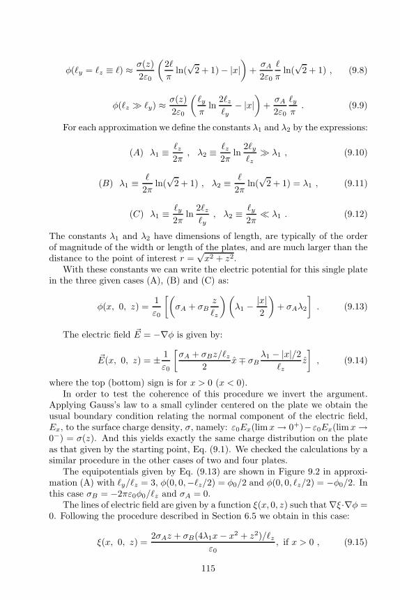
φ(ℓy = ℓz ≡ ℓ) ≈ σ(z)

2ε0

(

2ℓ

πln(

√2 + 1) − |x|

)

+σA2ε0

ℓ

πln(

√2 + 1) , (9.8)

φ(ℓz ≫ ℓy) ≈σ(z)

2ε0

(

ℓyπ

ln2ℓzℓy

− |x|)

+σA2ε0

ℓyπ. (9.9)

For each approximation we define the constants λ1 and λ2 by the expressions:

(A) λ1 ≡ ℓz2π

, λ2 ≡ ℓz2π

ln2ℓyℓz

≫ λ1 , (9.10)

(B) λ1 ≡ ℓ

2πln(

√2 + 1) , λ2 ≡ ℓ

2πln(

√2 + 1) = λ1 , (9.11)

(C) λ1 ≡ ℓy2π

ln2ℓzℓy

, λ2 ≡ ℓy2π

≪ λ1 . (9.12)

The constants λ1 and λ2 have dimensions of length, are typically of the orderof magnitude of the width or length of the plates, and are much larger than thedistance to the point of interest r =

√x2 + z2.

With these constants we can write the electric potential for this single platein the three given cases (A), (B) and (C) as:

φ(x, 0, z) =1

ε0

[(

σA + σBz

ℓz

)(

λ1 −|x|2

)

+ σAλ2

]

. (9.13)

The electric field ~E = −∇φ is given by:

~E(x, 0, z) = ± 1

ε0

[

σA + σBz/ℓz2

x∓ σBλ1 − |x|/2

ℓzz

]

, (9.14)

where the top (bottom) sign is for x > 0 (x < 0).In order to test the coherence of this procedure we invert the argument.

Applying Gauss’s law to a small cylinder centered on the plate we obtain theusual boundary condition relating the normal component of the electric field,Ex, to the surface charge density, σ, namely: ε0Ex(limx→ 0+)−ε0Ex(limx→0−) = σ(z). And this yields exactly the same charge distribution on the plateas that given by the starting point, Eq. (9.1). We checked the calculations by asimilar procedure in the other cases of two and four plates.

The equipotentials given by Eq. (9.13) are shown in Figure 9.2 in approxi-mation (A) with ℓy/ℓz = 3, φ(0, 0,−ℓz/2) = φ0/2 and φ(0, 0, ℓz/2) = −φ0/2. Inthis case σB = −2πε0φ0/ℓz and σA = 0.

The lines of electric field are given by a function ξ(x, 0, z) such that ∇ξ·∇φ =0. Following the procedure described in Section 6.5 we obtain in this case:

ξ(x, 0, z) =2σAz + σB(4λ1x− x2 + z2)/ℓz

ε0, if x > 0 , (9.15)

115

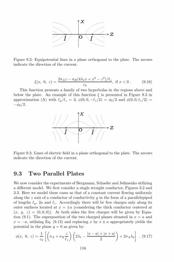
Figure 9.2: Equipotential lines in a plane orthogonal to the plate. The arrowsindicate the direction of the current.

ξ(x, 0, z) =2σAz − σB(4λ1x+ x2 − z2)/ℓz

ε0, if x < 0 . (9.16)

This function presents a family of two hyperbolas in the regions above andbelow the plate. An example of this function ξ is presented in Figure 9.3 inapproximation (A) with ℓy/ℓz = 3, φ(0, 0,−ℓz/2) = φ0/2 and φ(0, 0, ℓz/2) =−φ0/2.

Figure 9.3: Lines of electric field in a plane orthogonal to the plate. The arrowsindicate the direction of the current.

9.3 Two Parallel Plates

We now consider the experiments of Bergmann, Schaefer and Jefimenko utilizinga different model. We first consider a single straight conductor, Figures 3.2 and3.3. Here we model these cases as that of a constant current flowing uniformlyalong the z axis of a conductor of conductivity g in the form of a parallelepipedof lengths ℓy, 2a and ℓz. Accordingly there will be free charges only along itsouter surfaces located at x = ±a (considering the thick conductor centered at(x, y, z) = (0, 0, 0)). At both sides the free charges will be given by Equa-tion (9.1). The superposition of the two charged planes situated in x = a andx = −a, utilizing Eq. (9.13) and replacing x by x ± a appropriately yields thepotential in the plane y = 0 as given by:

φ(x, 0, z) =1

ε0

[(

σA + σBz

ℓz

)(

2λ1 −|x− a| + |x+ a|

2

)

+ 2σAλ2

]

. (9.17)

116

This potential can be seen in Figure 9.4 in approximation (A) with ℓy/ℓz =ℓz/2a = 6.5. With the boundary conditions φ(±a, 0, −ℓz/2) = φ0/2 andφ(±a, 0, ℓz/2) = −φ0/2 we have σB = −φ0ε0/(4λ1 − 2a) and σA = 0.

Figure 9.4: Equipotential lines in a plane orthogonal to two parallel platescarrying steady currents along the positive z direction.

The electric field is readily given by ~E = −∇φ:

~E(x > a, 0, z) =1

ε0

[(

σA + σBz

ℓz

)

x− σB2λ1 − x

ℓzz

]

, (9.18)

~E(−a < x < a, 0, z) = − 1

ε0σB

2λ1 − a

ℓzz , (9.19)

~E(x < −a, 0, z) = − 1

ε0

[(

σA + σBz

ℓz

)

x− σB2λ1 + x

ℓzz

]

. (9.20)

As expected, the electric field is constant in the region between the twoplates. This fact allows us to utilize the situation of two plates to model alsothe parallelepiped of sides ℓy and 2a carrying a steady current along the zdirection. The two plates already mentioned would be equivalent to the topand bottom plates of the parallelepiped located in the planes x = ±a.

The lines of electric field ξ(x, 0, z) such that ∇ξ · ∇φ = 0 can be obtainedby the method described before. They are given by the following equation:

ξ(x, 0, z) =

(2σAz + σB(4λ1x− x2 + z2)/ℓz)/ε0, x > a ,−σBax/ℓzε0, −a < x < a ,(2σAz − σB(4λ1x+ x2 − z2)/ℓz)/ε0, x < −a .

(9.21)

In Figure 9.5 we plot this function with the approximation ℓy/ℓz = ℓz/2a =6.5, in order to have similar dimensions as in Jefimenko’s experiment. Thistheoretical Figure is similar to Jefimenko’s experimental one, Figure 3.3.

9.4 Four Parallel Plates

We now wish to obtain plots similar to Figures 3.5 and 3.2 utilizing the paral-lelepiped model of this Chapter. We have essentially a transmission line in which

117

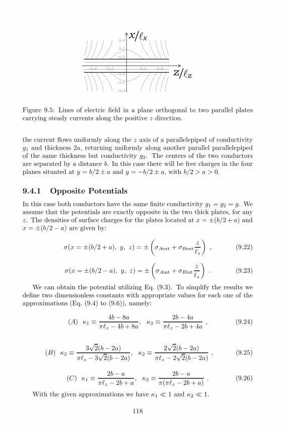
Figure 9.5: Lines of electric field in a plane orthogonal to two parallel platescarrying steady currents along the positive z direction.

the current flows uniformly along the z axis of a parallelepiped of conductivityg1 and thickness 2a, returning uniformly along another parallel parallelepipedof the same thickness but conductivity g2. The centers of the two conductorsare separated by a distance b. In this case there will be free charges in the fourplanes situated at y = b/2 ± a and y = −b/2 ± a, with b/2 > a > 0.

9.4.1 Opposite Potentials

In this case both conductors have the same finite conductivity g1 = g2 = g. Weassume that the potentials are exactly opposite in the two thick plates, for anyz. The densities of surface charges for the plates located at x = ±(b/2 + a) andx = ±(b/2 − a) are given by:

σ(x = ±(b/2 + a), y, z) = ±(

σAext + σBextz

ℓz

)

, (9.22)

σ(x = ±(b/2 − a), y, z) = ±(

σAint + σBintz

ℓz

)

. (9.23)

We can obtain the potential utilizing Eq. (9.3). To simplify the results wedefine two dimensionless constants with appropriate values for each one of theapproximations (Eq. (9.4) to (9.6)), namely:

(A) κ1 ≡ 4b− 8a

πℓz − 4b+ 8a, κ2 ≡ 2b− 4a

πℓz − 2b+ 4a, (9.24)

(B) κ2 ≡ 3√

2(b− 2a)

πℓz − 3√

2(b− 2a), κ2 ≡ 2

√2(b − 2a)

πℓz − 2√

2(b− 2a), (9.25)

(C) κ1 ≡ 2b− a

πℓz − 2b+ a, κ2 ≡ 2b− a

π(πℓz − 2b+ a). (9.26)

With the given approximations we have κ1 ≪ 1 and κ2 ≪ 1.

118

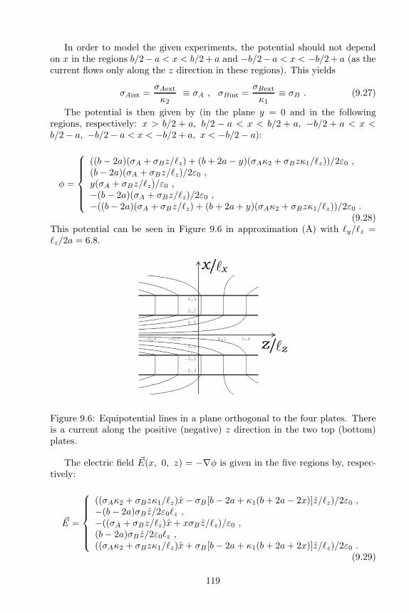
In order to model the given experiments, the potential should not dependon x in the regions b/2− a < x < b/2 + a and −b/2− a < x < −b/2 + a (as thecurrent flows only along the z direction in these regions). This yields

σAint =σAext

κ2≡ σA , σBint =

σBext

κ1≡ σB . (9.27)

The potential is then given by (in the plane y = 0 and in the followingregions, respectively: x > b/2 + a, b/2 − a < x < b/2 + a, −b/2 + a < x <b/2 − a, −b/2 − a < x < −b/2 + a, x < −b/2 − a):

φ =

((b − 2a)(σA + σBz/ℓz) + (b+ 2a− y)(σAκ2 + σBzκ1/ℓz))/2ε0 ,(b− 2a)(σA + σBz/ℓz)/2ε0 ,y(σA + σBz/ℓz)/ε0 ,−(b− 2a)(σA + σBz/ℓz)/2ε0 ,−((b− 2a)(σA + σBz/ℓz) + (b + 2a+ y)(σAκ2 + σBzκ1/ℓz))/2ε0 .

(9.28)This potential can be seen in Figure 9.6 in approximation (A) with ℓy/ℓz =ℓz/2a = 6.8.

Figure 9.6: Equipotential lines in a plane orthogonal to the four plates. Thereis a current along the positive (negative) z direction in the two top (bottom)plates.

The electric field ~E(x, 0, z) = −∇φ is given in the five regions by, respec-tively:

~E =

((σAκ2 + σBzκ1/ℓz)x− σB [b− 2a+ κ1(b+ 2a− 2x)]z/ℓz)/2ε0 ,−(b− 2a)σB z/2ε0ℓz ,−((σA + σBz/ℓz)x + xσB z/ℓz)/ε0 ,(b− 2a)σB z/2ε0ℓz ,((σAκ2 + σBzκ1/ℓz)x+ σB [b− 2a+ κ1(b+ 2a+ 2x)]z/ℓz)/2ε0 .

(9.29)

119

The lines of electric field, ξ(x, 0, z), are given for each region in Eq. (9.30):

ξ =

(2σAzκ2/κ1 + σB[[b+ 2a+ (b − 2a)/κ1]x− x2 + z2]/ℓz)/ε0 ,−σB(b− 2a)x/2ℓzε0 ,(2σAz − σB(x2 − z2)/ℓz)/ε0 ,σB(b− 2a)x/2ℓzε0 ,(2σAzκ2/κ1 − σB[[b+ 2a+ (b − 2a)/κ1]x− x2 + z2]/ℓz)/ε0 .

(9.30)

In Figure 9.7 we plot this function in the approximation (A) with ℓy/ℓz =ℓz/2a = 6.8. The upper plate has the potential at its boundaries given byφ(b/2 − a < x < b/2 + a, 0, −ℓz/2) = φ0/2 and φ(b/2 − a < x < b/2 +a, 0, ℓz/2) = 0, while the lower plate has the potential at its boundaries givenby φ(−b/2 − a < x < −b/2 + a, 0, −ℓz/2) = −φ0/2 and φ(−b/2 − a < x <−b/2 + a, 0, ℓz/2) = 0.

The relation between φ0 and the surface charges for this case is given byσA = ε0φ0/2(b− 2a) and σB = −ε0φ0/(b− 2a).

Figure 9.7: Lines of electric field in a plane orthogonal to the four plates. Thereis a current along the positive (negative) z direction in the two top (bottom)plates.

9.4.2 Perfect Conductor Plate

Now, suppose that the two lower plates (or the lower parallelepiped) are aperfect conductor, with zero resistivity. That is, suppose they are subjected tothe same constant potential φ(−b/2 − a < x < −b/2 + a, 0, z) = Φ in thewhole extension along the z axis, but still conducting a steady current. Thisexperimental result is shown at the right side of Figure 3.5 with g1 ≪ g2. Tomodel this case we consider four plates located at x = b/2 + a, x = b/2 − a,x = −b/2+a and x = −b/2−a. Their surface charges are given by, respectively,σ(x = b/2 + a, y, z) = σAb + σBbz/ℓz, σ(x = b/2 − a, y, z) = σAa + σBaz/ℓz,

120

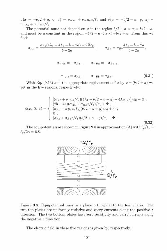
σ(x = −b/2 + a, y, z) = σ−Aa + σ−Baz/ℓz and σ(x = −b/2 − a, y, z) =σ−Ab + σ−Bbz/ℓz.

The potential must not depend on x in the region b/2 − a < x < b/2 + a,and must be a constant in the region −b/2 − a < x < −b/2 + a. From this wefind:

σAa =σAb(4λ1 + 4λ2 − b− 2a) − 2Φε0

b− 2a, σBa = σBb

4λ1 − b− 2a

b− 2a,

σ−Aa = −σAa , σ−Ba = −σBa ,

σ−Ab = σAb , σ−Bb = σBb . (9.31)

With Eq. (9.13) and the appropriate replacements of x by x± (b/2 ± a) weget in the five regions, respectively:

φ(x, 0, z) =

[(σAb + σBbz/ℓz)(4λ1 − b/2 − a− y) + 4λ2σAb]/ε0 − Φ ,(2b− 4a)(σAa + σBaz/ℓz)/ε0 + Φ ,(σAa + σBaz/ℓz)(b/2 − a+ y)/ε0 + Φ ,Φ ,(σAb + σBbz/ℓz)(b/2 + a+ y)/ε0 + Φ .

(9.32)The equipotentials are shown in Figure 9.8 in approximation (A) with ℓy/ℓz =

ℓz/2a = 6.8.

Figure 9.8: Equipotential lines in a plane orthogonal to the four plates. Thetwo top plates are uniformly resistive and carry currents along the positive zdirection. The two bottom plates have zero resistivity and carry currents alongthe negative z direction.

The electric field in these five regions is given by, respectively:

121

~E =

[(σAb + σBbz/ℓz)x− σBb(4λ1 − b/2 − a− x)z/ℓz]/ε0 ,−(b− 2a)σBaz/ℓzε0 ,−[(σAa + σBaz/ℓz)x+ σBa(b/2 − a+ x)z/ℓz]/ε0 ,~0 ,−[(σAb + σBbz/ℓz)x+ σBb(b/2 + a+ x)z/ℓz]/ε0 .

(9.33)

The lines of electric field are given by:

ξ(x, 0, z) =

(2σAbz + σBb((8λ1 − b− 2a)x− x2 + z2)/ℓz)/ε0 ,−σBb(b − 2a)x/2ℓzε0 ,(2σAaz − σBa((b− 2a)x+ x2 − z2)/ℓz)/ε0 ,−σBa(b− 2a)2/4ℓzε0 ,(2σAbz − σBb((b + 2a)x+ x2 − z2)/ℓz)/ε0 .

(9.34)

They are shown in Figure 9.9 with the given approximation and the samedimensions as in Figure 9.7. The constant potential in the lower plate isΦ = −φ0/2. Once more there is a reasonable match with Jefimenko’s experi-mental result, the right side of Figure 3.5, especially in the region between theparallelepipeds.

Figure 9.9: Lines of electric field in a plane orthogonal to the four plates. Thetwo top plates are uniformly resistive and carry currents along the positive zdirection. The two bottom plates have zero resistivity and carry currents alongthe negative z direction.

122

Chapter 10

Resistive Strip

10.1 The Problem

Here we consider a constant current flowing uniformly through the surface ofa stationary and resistive straight strip. Our goal is to calculate the potentialφ and electric field ~E everywhere in space and the surface charge distributionσ along the strip that creates this electric field. We follow essentially the workpublished in 2003 [223].

We consider a strip in the x = 0 plane localized in the region −a < y < a and−ℓ/2 < z < ℓ/2, such that ℓ≫ a > 0. The medium around the strip is taken tobe air or vacuum. The constant current I flows uniformly along the positive zdirection with a surface current density given by ~K = Iz/2a (see Fig. 10.1). ByOhm’s law this uniform current distribution is related to a spatially constantelectric field along the surface of the strip. In the steady state this electric fieldcan be related to the potential by ~E = −∇φ. This relation means that along thestrip the potential is a linear function of z and independent of y. The problemcan then be solved by finding the solution of Laplace’s equation ∇2φ = 0 inempty space and applying the boundary conditions.

Figure 10.1: A resistive strip of width 2a and length ℓ with a steady and uniformsurface current density ~K along the positive z direction.

123

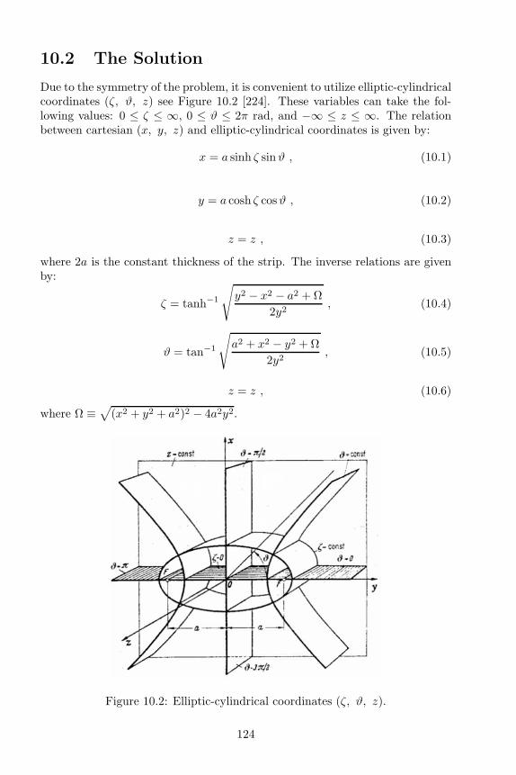
10.2 The Solution

Due to the symmetry of the problem, it is convenient to utilize elliptic-cylindricalcoordinates (ζ, ϑ, z) see Figure 10.2 [224]. These variables can take the fol-lowing values: 0 ≤ ζ ≤ ∞, 0 ≤ ϑ ≤ 2π rad, and −∞ ≤ z ≤ ∞. The relationbetween cartesian (x, y, z) and elliptic-cylindrical coordinates is given by:

x = a sinh ζ sinϑ , (10.1)

y = a cosh ζ cosϑ , (10.2)

z = z , (10.3)

where 2a is the constant thickness of the strip. The inverse relations are givenby:

ζ = tanh−1

√

y2 − x2 − a2 + Ω

2y2, (10.4)

ϑ = tan−1

√

a2 + x2 − y2 + Ω

2y2, (10.5)

z = z , (10.6)

where Ω ≡√

(x2 + y2 + a2)2 − 4a2y2.

Figure 10.2: Elliptic-cylindrical coordinates (ζ, ϑ, z).

124

Laplace’s equation in this coordinate system is given by:

∇2φ =1

a2(cosh2 ζ − cos2 ϑ)

(

∂2φ

∂ζ2+∂2φ

∂ϑ2

)

+∂2φ

∂z2= 0 . (10.7)

A solution of Eq. (10.7) can be obtained by separation of variables in the formφ(ζ, ϑ, z) = H(ζ)Φ(ϑ)Z(z):

H ′′ − (α2 + α3a2 cosh2 ζ)H = 0 , (10.8)

Φ′′ + (α2 + α3a2 cos2 ϑ)Φ = 0 , (10.9)

Z ′′ + α3Z = 0 , (10.10)

where α2 and α3 are constants.For the long strip being considered here, it is possible to neglect boundary

effects near z = ±ℓ/2. It has already been proved that in this case the potentialmust be a linear function of z, not only over the strip, but also over all space.See Section 5.4. This condition means that α3 = 0. There are then two possiblesolutions for Φ(ϑ). If α2 = 0, then Φ = C1 + C2ϑ; if α2 6= 0, then Φ =C3 sin(

√α2ϑ) + C4 cos(

√α2ϑ), where C1 to C4 are constants. Along the strip

we have x = 0, and y2 ≤ a2, which means that Ω = a2 − y2, ζ = 0 andϑ = tan−1

√

(a2 − y2)/y2. We are assuming that the potential does not dependon y along the strip. This independence and the relation between y and ϑ meansthat the potential will not depend on ϑ as well. Thus a non-trivial solution forΦ can only exist if α2 = 0, C2 = 0, and Φ = constant for all ϑ. The solution forH with α2 = α3 = 0 will be then a linear function of ζ. The general solution ofthe problem is then given by:

φ = (A1ζ −A2)(

φA + φBz

ℓ

)

=

(

A1 tanh−1

√

y2 − x2 − a2 + Ω

2y2− A2

)

(

φA + φBz

ℓ

)

. (10.11)

The electric field ~E = −∇φ takes the form:

~E = −A1

( |y|x√

2

Ω√

y2 − x2 − a2 + Ωx

+|y|√

y2 − x2 − a2 + Ω

y√

2Ωy

)

(

φA + φBz

ℓ

)

− φBℓ

(

A1 tanh−1

√

y2 − x2 − a2 + Ω

2y2−A2

)

z , (10.12)

125

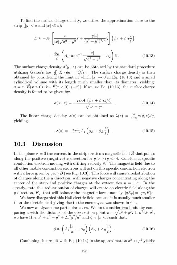
To find the surface charge density, we utilize the approximation close to thestrip (|y| < a and |x| ≪ a):

~E ≈ −A1

[

x

|x|√

a2 − y2x+

y|x|(a2 − y2)3/2

y

]

(

φA + φBz

ℓ

)

− φBℓ

(

A1 tanh−1 |x|√

a2 − y2−A2

)

z . (10.13)

The surface charge density σ(y, z) can be obtained by the standard procedure

utilizing Gauss’s law∫

∫

S~E · d~a = Q/ε0. The surface charge density is then

obtained by considering the limit in which |x| → 0 in Eq. (10.13) and a smallcylindrical volume with its length much smaller than its diameter, yielding:σ = ε0[ ~E(x > 0) · x− ~E(x < 0) · (−x)]. If we use Eq. (10.13), the surface chargedensity is found to be given by:

σ(x, z) = −2ε0A1(φA + φBz/ℓ)√

a2 − y2. (10.14)

The linear charge density λ(z) can be obtained as λ(z) =∫ a

−a σ(y, z)dy,yielding

λ(z) = −2πε0A1

(

φA + φBz

ℓ

)

. (10.15)

10.3 Discussion

In the plane x = 0 the current in the strip creates a magnetic field ~B that pointsalong the positive (negative) x direction for y > 0 (y < 0). Consider a specificconduction electron moving with drifting velocity ~vd. The magnetic field due toall other mobile conduction electrons will act on this specific conduction electronwith a force given by q~vd× ~B (see Fig. 10.3). This force will cause a redistributionof charges along the y direction, with negative charges concentrating along thecenter of the strip and positive charges at the extremities y = ±a. In thesteady-state this redistribution of charges will create an electric field along they direction, Ey , that will balance the magnetic force, namely, |qEy | = |qvdB|.

We have disregarded this Hall electric field because it is usually much smallerthan the electric field giving rise to the current, as was shown in 6.4.

We now analyze some particular cases. We first consider two limits by com-paring a with the distance of the observation point ρ =

√

x2 + y2. If a2 ≫ ρ2,we have Ω ≈ a2 + x2 − y2 + 2x2y2/a2 and ζ ≈ |x|/a, such that:

φ ≈(

A1|x|a

−A2

)

(

φA + φBz

ℓ

)

. (10.16)

Combining this result with Eq. (10.14) in the approximation a2 ≫ ρ2 yields:

126

Figure 10.3: Magnetic field ~B along the strip due to the current along thepositive z direction. There is a magnetic force pointing toward the axis actingupon the conduction electrons.

φ ≈ σ(z)

2ε0

(

aA2

A1− |x|

)

. (10.17)

This result coincides with Eq. (9.9) considering aA2/A1 = (ℓy/π) ln(2ℓz/ℓy) andσA = 0. This was expected because a strip with ℓ2 ≫ a2 ≫ ρ2 is equivalent toa large plate.

This Equation is also equivalent to Eq. (6.26) with A2/A1 = ln(ℓ/a) exceptby an overall factor of 2. This was once more to be expected. The electrostaticpotential at a distance d from a charged plate is given by φ = φ0 − σd/2ε0,where φ0 is an arbitrary constant and σ is the total density of surface charge,half of it in each side of the charged plane. On the other hand, the electrostaticpotential just outside a closed charged conductor (at a distance d from it) isgiven φ = φ1 − σd/ε0, where φ1 is an arbitrary constant and σ here is thesurface charge density at the point in which the potential is being estimated,while the internal potential has the constant value φ1. That is, when we close anopen charged conducting surface, the charges in the internal side migrate to theexternal side. The magnitude of the electric field just outside the closed surfaceis twice the electric field close to a large charged plane, supposing the same localcharge density in both cases. As we have seen here, the same happens with thesurface charges when a current flows along the resistive surface.

On the other hand, if a2 ≪ ρ2, we have Ω ≈ ρ2 + a2 − 2a2y2/ρ2 andζ ≈ ln(ρ/a). Utilizing these results in Eq. (10.11) combined with Eq. (10.15)yields:

φ ≈ λ(z)

2πε0

(

A2

A1− ln

ρ

a

)

. (10.18)

This result coincides with Eq. (6.11) with A2/A1 = ln(ℓ/a), where ℓ is the typ-ical length of the wire or strip being considered, with ℓ≫ a. This is reasonablebecause Eq. (6.11) corresponds to the potential outside a long straight cylindri-cal wire carrying a constant current. At a point far from the axis of the stripboth results coincide as they must.

127

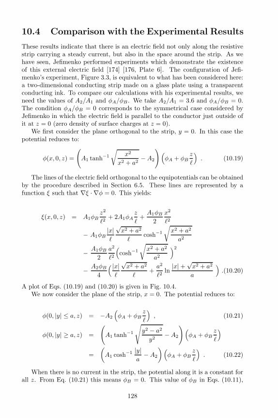
10.4 Comparison with the Experimental Results

These results indicate that there is an electric field not only along the resistivestrip carrying a steady current, but also in the space around the strip. As wehave seen, Jefimenko performed experiments which demonstrate the existenceof this external electric field [174] [176, Plate 6]. The configuration of Jefi-menko’s experiment, Figure 3.3, is equivalent to what has been considered here:a two-dimensional conducting strip made on a glass plate using a transparentconducting ink. To compare our calculations with his experimental results, weneed the values of A2/A1 and φA/φB . We take A2/A1 = 3.6 and φA/φB = 0.The condition φA/φB = 0 corresponds to the symmetrical case considered byJefimenko in which the electric field is parallel to the conductor just outside ofit at z = 0 (zero density of surface charges at z = 0).

We first consider the plane orthogonal to the strip, y = 0. In this case thepotential reduces to:

φ(x, 0, z) =

(

A1 tanh−1

√

x2

x2 + a2−A2

)

(

φA + φBz

ℓ

)

. (10.19)

The lines of the electric field orthogonal to the equipotentials can be obtainedby the procedure described in Section 6.5. These lines are represented by afunction ξ such that ∇ξ · ∇φ = 0. This yields:

ξ(x, 0, z) = A1φBz2

ℓ2+ 2A1φA

z

ℓ+A1φB

2

x2

ℓ2

− A1φB|x|ℓ

√x2 + a2

ℓcosh−1

√

x2 + a2

a2

− A1φB2

a2

ℓ2

(

cosh−1

√

x2 + a2

a2

)2

− A2φB4

( |x|ℓ

√x2 + a2

ℓ+a2

ℓ2ln

|x| +√x2 + a2

a

)

.(10.20)

A plot of Eqs. (10.19) and (10.20) is given in Fig. 10.4.We now consider the plane of the strip, x = 0. The potential reduces to:

φ(0, |y| ≤ a, z) = −A2

(

φA + φBz

ℓ

)

, (10.21)

φ(0, |y| ≥ a, z) =

(

A1 tanh−1

√

y2 − a2

y2−A2

)

(

φA + φBz

ℓ

)

=

(

A1 cosh−1 |y|a

−A2

)

(

φA + φBz

ℓ

)

. (10.22)

When there is no current in the strip, the potential along it is a constant forall z. From Eq. (10.21) this means φB = 0. This value of φB in Eqs. (10.11),

128

Figure 10.4: Equipotentials (dashed lines) and lines of electric field (continuouslines) in a plane orthogonal to the plane of the strip.

(10.12) and (10.14) reduces these equations to the known electrostatic solutionof a strip charged to a constant potential [225].

By a similar procedure, the lines of electric field for the plane x = 0 aregiven by:

ξ(0, |y| ≤ a, z) = A2φBay

ℓ2, (10.23)

ξ(0, |y| ≥ a, z) = A1φBz2

ℓ2+ 2A1φA

z

ℓ+A1φB

2

y2

ℓ2

− A1φB|y|ℓ

√

y2 − a2

ℓcosh−1 |y|

a

+A1φB

2

a2

ℓ2

(

cosh−1 |y|a

)

− A2φB4

( |y|ℓ

√

y2 − a2

ℓ

− a2

ℓ2ln

|y| +√

y2 − a2

a

)

. (10.24)

A plot of Eqs. (10.21) to (10.24) is presented in Fig. 10.5.Figure 10.6 presents the theoretical electric field lines overlaid on the exper-

imental result of Jefimenko, Figure 3.3.In Fig. 10.7 the experimental result of Jefimenko, Barnett and Kelly, Fig-

ure 3.10, is overlaid on the equipotential lines calculated utilizing Eqs. (10.23)and (10.24) with A2/A1 = 3.0 and φA/φB = 0. The agreement is not as good

129

Figure 10.5: Equipotentials (dashed lines) and lines of electric field (continuouslines) in the plane of the strip.

Figure 10.6: Theoretical lines of electric field overlaid on the experimental linesobtained by Jefimenko.

as in our previous figure for two reasons: One reason is that our calculationsare for a two-dimensional configuration, while the experiment of Jefimenko, Bar-nett and Kelly [177] was performed in a three-dimensional rectangular chamber.The second reason is that in the grass seed experiment [174], the ratio of thelength to the width of the conductor was 7, but in the second experiment [177],this ratio was only 2, which means that boundary effects near z = ℓ/2 andz = −ℓ/2 are more important. These boundary effects were not considered inour calculations.

130

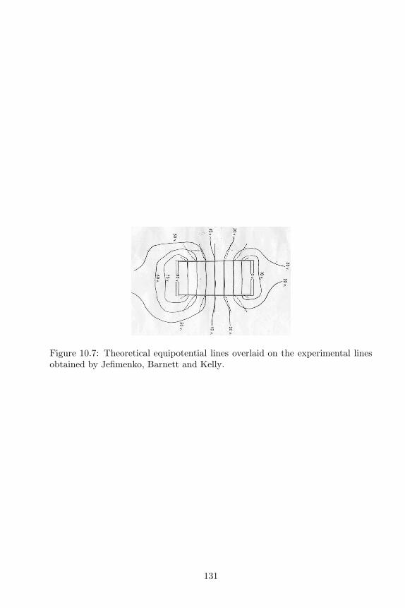
Figure 10.7: Theoretical equipotential lines overlaid on the experimental linesobtained by Jefimenko, Barnett and Kelly.

131

132

Part III

Curved Conductors

133

In this third Part of the book we consider resistive conductors carryingsteady currents along curved paths. Russell’s theorem, discussed in Section 5.4,is no longer valid due to the curvature of the wire. Three cases in particularwill be discussed here, the azimuthal current in an infinite cylindrical shell,the azimuthal current over the surface of a spherical shell, and the azimuthalcurrent in a toroidal conductor. These cases can still be solved analytically, andtheir solutions clarify some important aspects of surface charges in conductorscarrying steady currents.

135

136

Chapter 11

Resistive Cylindrical Shell

with Azimuthal Current

11.1 Configuration of the Problem

The subject of this Chapter has been discussed mainly by Jefimenko [175, Prob-lem 9.33 and Figure 14.7] [176, p. 318], Heald [226] and Griffiths [16, p. 279].We follow these approaches here.

An infinite homogeneous resistive cylindrical shell of radius a has its axiscoinciding with the z direction. We utilize cylindrical coordinates (ρ, ϕ, z)

with origin at the center of the shell, with ρ =√

x2 + y2 being the distance tothe z axis. There is a narrow slot along its entire length located at (ρ, ϕ, z) =(a, π, z). An idealized line battery in the slot maintains its terminals locatedat ϕ = ±π rad with the constant potentials φ = ±φB/2, respectively. SeeFigure 11.1.

Figure 11.1: Configuration of the problem.

In accordance with Ohm’s law the potential along the surface of the cylin-drical shell is then given by

137

φ(a, ϕ, z) = φBϕ

2π. (11.1)

11.2 Potential and Electric Field

The potential inside and outside the cylindrical shell satisfies Laplace’s equation∇2φ = 0:

1

ρ

∂

∂ρ

(

ρ∂φ

∂ρ

)

+1

ρ2

∂2φ

∂ϕ2+∂2φ

∂z2= 0 . (11.2)

The solution should be independent of z. Trying a solution in terms ofseparation of variables φ(ρ, ϕ, z) = R(ρ)Φ(ϕ) yields

Φ′′ +m2Φ = 0 , (11.3)

ρd

dρ

(

ρdR

dρ

)

−m2R = 0 , (11.4)

where m is a constant. The solutions of these equations if m = 0 are Φ(ϕ) =A0 + B0ϕ and R(ρ) = C0 ln ρ +D0. If m 6= 0 we have φ(ϕ) = Am cos(mϕ) +Bm sin(mϕ) and R(ρ) = Cmρ

−m + Dmρm. The solutions must be periodic in

ϕ, i.e., Φ(ϕ+ 2π) = Φ(ϕ). This means that B0 = 0 and m = 1, 2, 3, ...The internal and external solutions, with appropriate coefficients, are then

given by

φ(ρ ≤ a, ϕ, z) = A0i (C0i ln ρ+D0i)

+

∞∑

m=1

[Ami cos(mϕ) +Bmi sin(mϕ)][

Cmiρ−m +Dmiρ

m]

, (11.5)

φ(ρ ≥ a, ϕ, z) = A0e (C0e ln ρ+D0e)

+

∞∑

m=1

[Ame cos(mϕ) +Bme sin(mϕ)][

Cmeρ−m +Dmeρ

m]

, (11.6)

We specify finite solutions when ρ→ 0. This means that C0i = C1i = C2i =... = 0. We also specify solutions in which the potential goes to zero whenρ → ∞. This means that C0e = D0e = D1e = D2e = ... = 0. Our solutions inthese two regions reduce to

φ(ρ ≤ a, ϕ, z) = A0iD0i +

∞∑

m=1

[AmiDmi cos(mϕ) +BmiDmi sin(mϕ)] ρm ,

(11.7)

138

φ(ρ ≥ a, ϕ, z) =∞∑

m=1

[AmeCme cos(mϕ) +BmeCme sin(mϕ)]1

ρm. (11.8)

The potential must be continuous in ρ = a. This means that A0iD0i = 0,AmiDmia

m = AmeCmea−m andBmiDmia

m = BmeCmea−m. Defining AmiDmi ≡

Gm and BmiDmi ≡ Hm yields

φ(ρ ≤ a, ϕ, z) =

∞∑

m=1

[Gm cos(mϕ) +Hm sin(mϕ)] ρm , (11.9)

φ(ρ ≥ a, ϕ, z) =∞∑

m=1

[Gm cos(mϕ) +Hm sin(mϕ)]a2m

ρm. (11.10)

Now we need to apply the boundary condition at ρ = a, Eq. (11.1). To thisend we employ the Fourier expansion of ϕ, which is valid for −π rad < ϕ < π rad:

ϕ = 2

[ ∞∑

m=1

(−1)m−1 sin(mϕ)

m

]

. (11.11)

Comparing Eqs. (11.9) and (11.10) at ρ = a with Eqs. (11.1) and (11.11)yields Gm = 0 and Hma

m = φB(−1)m+1/πm:

φ(ρ ≤ a, ϕ, z) = −φBπ

[ ∞∑

m=1

(−1)m(ρ

a

)m sin(mϕ)

m

]

, (11.12)

φ(ρ ≥ a, ϕ, z) = −φBπ

[ ∞∑

m=1

(−1)m(

a

ρ

)msin(mϕ)

m

]

. (11.13)

These two series can be put in closed form [226]:

φ(ρ ≤ a, ϕ, z) =φBπ

tan−1 ρ sinϕ

a+ ρ cosϕ=φBπ

tan−1 y

a+ x=φBπψ , (11.14)

φ(ρ ≥ a, ϕ, z) =φBπ

tan−1 a sinϕ

ρ+ a cosϕ=φBπ

tan−1 ay

x2 + ax+ y2, (11.15)

where ψ is the polar angle about the slot as the axis.The equipotentials given by these equations are represented in Figure 11.2.The lines of electric field given by the function ξ(x, y) such that ∇ξ ·∇φ = 0

can be obtained by the method described in Section 6.5. For the region ρ < athis function is given by

ξ(x, y) = φB2ax+ x2 + y2

a2. (11.16)

These are circular arcs centered on the battery given by the following equation(for a particular ξo):

139

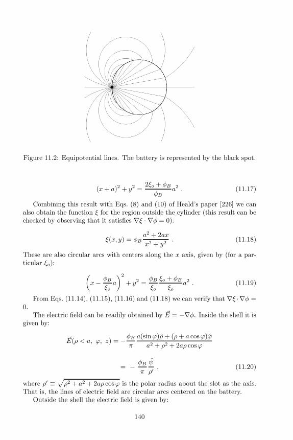
Figure 11.2: Equipotential lines. The battery is represented by the black spot.

(x+ a)2 + y2 =2ξo + φBφB

a2 . (11.17)

Combining this result with Eqs. (8) and (10) of Heald’s paper [226] we canalso obtain the function ξ for the region outside the cylinder (this result can bechecked by observing that it satisfies ∇ξ · ∇φ = 0):

ξ(x, y) = φBa2 + 2ax

x2 + y2. (11.18)

These are also circular arcs with centers along the x axis, given by (for a par-ticular ξo):

(

x− φBξoa

)2

+ y2 =φBξo

ξo + φBξo

a2 . (11.19)

From Eqs. (11.14), (11.15), (11.16) and (11.18) we can verify that ∇ξ ·∇φ =0.

The electric field can be readily obtained by ~E = −∇φ. Inside the shell it isgiven by:

~E(ρ < a, ϕ, z) = −φBπ

a(sinϕ)ρ+ (ρ+ a cosϕ)ϕ

a2 + ρ2 + 2aρ cosϕ

= − φBπ

ψ

ρ′, (11.20)

where ρ′ ≡√

ρ2 + a2 + 2aρ cosϕ is the polar radius about the slot as the axis.That is, the lines of electric field are circular arcs centered on the battery.

Outside the shell the electric field is given by:

140

~E(ρ > a, ϕ, z) =φBπ

a

ρ

ρ(sinϕ)ρ− (a+ ρ cosϕ)ϕ

a2 + ρ2 + 2aρ cosϕ, (11.21)

with magnitude | ~E| = φBa/πρρ′.

At the surface of the shell, ρ = a, Eqs. (11.20) and (11.21) yield the sametangential component:

Eϕ(a, ϕ, z) = − φB2πa

. (11.22)

This is the correct result arising from Eq. (11.1), namely, E = ∆φ/L, where∆φ ≡ φB is the potential difference generated by the battery and L ≡ 2πa isthe length described by the electrons around the circuit.

The lines of electric field are represented in Figure 11.3.

Figure 11.3: Lines of electric field. The battery is represented by the black spot.

11.3 Surface Charge Densities

The surface charge densities inside and outside the hollow shell (that is, alongthe internal and external surfaces), σi and σo, are obtained utilizing Gauss’slaw. They have the same value and are given by

σi = σo =ε0φB2πa

tanϕ

2=ε0φB2πa

tanψ . (11.23)

A plot of this surface charge density as a function of ϕ is shown in Figure 11.4.The total charge density σt is given by

σt = σi + σo =ε0φBπa

tanϕ

2=ε0φBπa

tanψ . (11.24)

141

Figure 11.4: Surface charge densities σ ≡ σi = σo inside and outside the hollowshell as a function of the azimuthal angle ϕ, according to Eq. (11.23) [226].

Expanding Eq. (11.23) for ϕ ≪ 1 rad and utilizing Eqs. (11.1) and (11.11)yields:

σi(ϕ≪ 1 rad) = σo(ϕ≪ 1 rad) ≈ ε0φBϕ

4πa=ε0φ

2a. (11.25)

This result coincides with Eq. (9.7) when we are over the plate (x = 0) andσA = 0, if we equate the circumference of the cylindrical shell here (2πa) withthe longitudinal length ℓz of the plate of Section 9.2, as expected. The surfacecharge density which appears in Eq. (9.7) is the total charge density due to thecharges in both sides of the plate, analogous to σi + σo of Eq. (11.25).

On the other hand, for ϕ = (π ± δ) rad, with 0 < δ ≪ 1 (that is, close toϕ = π rad) we have:

σi = σo ≈ ∓ε0φBπaδ

= ∓ε0φBπs

. (11.26)

Here s ≡ aδ is the distance along the surface of the cylindrical shell to theline battery. This is an important result which shows that the surface chargedensity diverges inversely proportional to the distance from the line battery inthis idealized case.

Eq. (11.23) indicates that in regions close to the battery the surface chargedensity is no longer a linear function of the longitudinal coordinate (in this casethe arc aϕ) of the resistive conductor. It is linear only close to ϕ = 0 rad butincreases nonlinearly (that is, it is not proportional to aϕ) toward the battery.See Figure 11.4. This nonlinearity should also occur in straight conductors whenwe are close to the battery. This has been confirmed in 2004 and 2005 [205, 222].

Eqs. (11.14) to (11.26) indicate that several functions are proportional tothe emf of the battery, namely: the internal and external potential and electricfield, as well as the surface charge densities in the internal and external walls.That is, they are proportional to the voltage φ(π) − φ(−π) = φB between theterminals of the battery. Suppose we have two cylindrical shells 1 and 2 ofthe same radius but with different resistivities. If we connect only shell 1 withbattery B and later on if we connect only shell 2 with the same battery B(assuming the battery has not lost its power), different steady currents will flow

142

in each shell, as they have different resistivities. But the internal and externalpotentials, electric fields and surface charge densities will be the same in bothcases. This again illustrates that the electric field outside a resistive conductorcarrying a steady current is proportional to the voltage to which it is subjected.The importance of the present case is that this has been shown in a situation inwhich we were able to find an exact analytical solution of all magnitudes. Thatis, this external electric field does not depend directly upon the current flowingin the circuit. After all, the electric field was found to be the same even whendifferent currents flow in two circuits connected by the same emf. In order toobserve the effects of the external electric field, it is most important to workwith circuits connected to high voltage sources, as this field is proportional tothe applied emf.

11.4 Representation in Fourier Series

Our solution of the potential in terms of Fourier series was presented in Eqs. (11.12)and (11.13). These series can be put in closed form. See Eqs. (11.14) and(11.15). If this were not possible, we could continue to utilize the Fourier series

representation obtaining the electric field ~E = −∇φ in the form

~E(ρ < a, ϕ, z) =φBπρ

∞∑

m=1

(−ρa

)m

[sin(mϕ)ρ+ cos(mϕ)ϕ]

, (11.27)

~E(ρ > a, ϕ, z) = −φBπρ

∞∑

m=1

(−aρ

)m

[sin(mϕ)ρ− cos(mϕ)ϕ]

. (11.28)

From these two equations the tangential component of the electric field atρ = a is given by:

Eϕ(a, ϕ, z) =φBπa

[ ∞∑

m=1

(−1)m cos(mϕ)

]

. (11.29)

This is a divergent series. This happens with the differentiation of some Fourierseries [202, Section 14.4]. By differentiating both sides of Eq. (11.11) we obtain

1 = 2

[ ∞∑

m=1

(−1)m−1 cos(nϕ)

]

. (11.30)

While Eq. (11.11) is convergent, the latter series is divergent. But if we disre-gard this and apply Eq. (11.30) into Eq. (11.29) we obtain the same result asEq. (11.22). And this is a reasonable result.

Figure 11.5 is a plot of

143

f(ϕ) ≡∞∑

m=1

(−1)m−1 cos(nϕ) , (11.31)

including 100 terms in the summation. The oscillations are due to the divergentcharacter of this series representation, although we can see that the curve oscil-lates around the constant value of f(ϕ) = 1/2, which was expected accordingto Eq. (11.30).

Figure 11.5: Plot of Eq. (11.31) including 100 terms in the summation. Theoscillations are due to the divergent character of this series. The bold line is aplot of the constant 1/2 as expected by Eq. (11.30).

In order to deal with a divergent Fourier series, we thought of applying anaverage approach. In particular, at each angle ϕi we consider the average valueof a generic function g(ϕ), g(ϕi), namely:

g(ϕi) ≡1

∆ϕ

∫ ϕi+∆ϕ/2

ϕi−∆ϕ/2

g(ϕ)dϕ . (11.32)

The value of ∆ϕ is typically taken as the whole interval in which we are plottingg(ϕ) divided by the number of terms we are including in the summation. Forinstance, if we are plotting a function g(ϕ) in the interval ϕ = −π rad to ϕ = πrad and we include 100 terms in the Fourier series expansion of g(ϕ), then∆ϕ = (2π/100) rad.

Figure 11.6 is a plot of f(ϕ) obtained from this averaging approach utilizingEq. (11.31). From this Figure we can see that f(ϕ) coincides with the expectedvalue of 1/2, indicating the correctness of this averaging procedure.

The surface charge densities inside and outside the shell can be obtainedfrom Gauss’s law. From Eqs. (11.27) and (11.28) this yields:

144

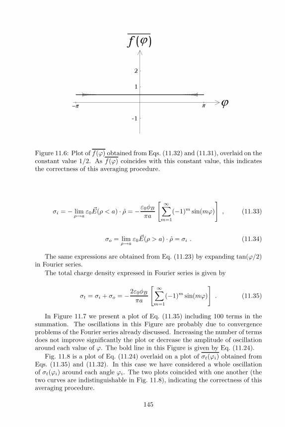
Figure 11.6: Plot of f(ϕ) obtained from Eqs. (11.32) and (11.31), overlaid on theconstant value 1/2. As f(ϕ) coincides with this constant value, this indicatesthe correctness of this averaging procedure.

σi = − limρ→a

ε0 ~E(ρ < a) · ρ = −ε0φBπa

[ ∞∑

m=1

(−1)m sin(mϕ)

]

, (11.33)

σo = limρ→a

ε0 ~E(ρ > a) · ρ = σi . (11.34)

The same expressions are obtained from Eq. (11.23) by expanding tan(ϕ/2)in Fourier series.

The total charge density expressed in Fourier series is given by

σt = σi + σo = −2ε0φBπa

[ ∞∑

m=1

(−1)m sin(mϕ)

]

. (11.35)

In Figure 11.7 we present a plot of Eq. (11.35) including 100 terms in thesummation. The oscillations in this Figure are probably due to convergenceproblems of the Fourier series already discussed. Increasing the number of termsdoes not improve significantly the plot or decrease the amplitude of oscillationaround each value of ϕ. The bold line in this Figure is given by Eq. (11.24).

Fig. 11.8 is a plot of Eq. (11.24) overlaid on a plot of σt(ϕi) obtained fromEqs. (11.35) and (11.32). In this case we have considered a whole oscillationof σt(ϕi) around each angle ϕi. The two plots coincided with one another (thetwo curves are indistinguishable in Fig. 11.8), indicating the correctness of thisaveraging procedure.

145

Figure 11.7: Total surface charge density σt = σi + σo of an infinite resistivecylindrical shell carrying a steady azimuthal current as a function of the angleϕ. The bold line is a plot of the closed form solution of σt(ϕ), Eq. (11.24), whilethe oscillatory line is a plot of σt(ϕ) expressed in a Fourier series, Eq. (11.35).

Figure 11.8: Total surface charge density σt. The summation that appears as anoscillation in Fig. 11.7, given by Eq. (11.35), is smoothed out by taking the meanvalue for each point of its surroundings (in this case, a whole oscillation aroundeach point), utilizing Eq. (11.32). The closed analytical form, Eq. (11.24), isoverlaid on it. Both plots coincide with one another, indicating the correctnessof this averaging procedure.

11.5 Lumped Resistor

Heald also considered a lumped resistor, i.e., a cylindrical shell of finite resistiv-ity for −α < ϕ < α and zero resistivity outside this region [226]. The potentialat the shell was given by

146

φ(a, ϕ, z) =∞∑

k=1

Ak sin(kϕ) . (11.36)

Here the coefficients Ak are given by:

Ak =φBπ

[∫ α

0

ϕ

αsin(kϕ)dϕ +

∫ π

α

sin(kϕ)dϕ

]

=φBπ

[

(−1)k−1

k+

sin(kϕ)

k2α

]

. (11.37)

The potential inside and outside the shell is given by, respectively:

φ(ρ ≤ a, ϕ, z) =φBπ

[

tan−1 ρ sinϕ

a+ ρ cosϕ

+∞∑

k=1

ρ

a

k sin(kα)

k2αsin(kϕ)

]

, (11.38)

φ(ρ ≥ a, ϕ, z) =φBπ

[

tan−1 a sinϕ

ρ+ a cosϕ

+

∞∑

k=1

a

ρ

k sin(kα)

k2αsin(kϕ)

]

. (11.39)

The equipotentials for this case of lumped resistor are represented in Fig-ure 11.9.

Figure 11.9: Equipotential lines for the lumped resistor.

147

Figure 11.10: Lines of electric field for the lumped resistor.

The electric field lines are represented in Figure 11.10.

The internal and external surface charge densities are again equal. In thiscase they are given by:

σi = σo =ε0φB2πa

[

tanϕ

2+

∞∑

k=1

2sin(kα)

kαsin(kϕ)

]

=ε0φB2πa

[

tanϕ

2+

1

αln | sin[(ϕ+ α)/2]

sin[(ϕ− α)/2]|]

. (11.40)

In this case the surface charge densities diverge not only at the battery butalso at the discontinuity in the resistivity of the shell, as in Figure 11.11.

Figure 11.11: Densities of surface charge σ ≡ σi = σo along the internal andexternal surfaces of the hollow lumped resistor (continuous line) as a functionof the azimuthal angle, as given by Eq. (11.40). The dashed line represents theprevious case of a uniformly resistive conductor.

148

Another qualitative discussion of lumped resistors can be found in the bookof Chabay and Sherwood [166, Section 18.6]. Their analysis is extremely didacticand helpful.

149

150

Chapter 12

Resistive Spherical Shell

with Azimuthal Current

12.1 Introduction

Our goal in this chapter is to consider a steady azimuthal current flowing in aresistive spherical shell [227]. The mathematical difficulty is intermediate be-tween the infinite cylindrical shell which we considered in the previous Chapterand the toroidal conductor which is the subject of the next Chapter. The im-portance of the present case is that we can obtain exact analytical solutions forthe external and internal distribution of surface charges, potential and electricfield which are not as complex as in the toroidal conductor. Despite this factthey show clearly the existence of an electric field outside a resistive conductorbounded in a finite volume of space. To the best of our knowledge this case hasnever been treated before by other authors.

12.2 Description of the Problem

Consider a resistive spherical shell of radius a, centered at the origin. Wesuppose an idealized linear battery located along a meridian of the shell (likeGreenwich Meridian) and maintaining a constant potential difference betweenits left and right sides. See Figure 12.1.

That is, the battery is a semi-circumference in the plane y = 0 with its ex-tremities at (x, y, z) = (0, 0,±a) and central point along the semi-circumferenceat (x, y, z) = (−a, 0, 0). Utilizing spherical coordinates (r, θ, ϕ) the linear bat-tery is then located at (a, θ, π). We suppose that the potential difference gen-erated by the battery does not depend upon the polar angle θ. The batterygenerates a steady current flowing along the shell in the azimuthal direction−ϕ. See Figs. 12.1 and 12.2. The medium inside and outside the spherical shellis supposed to be air or vacuum.

151

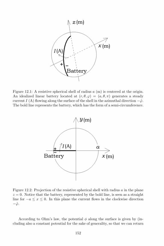
Figure 12.1: A resistive spherical shell of radius a (m) is centered at the origin.An idealized linear battery located at (r, θ, ϕ) = (a, θ, π) generates a steadycurrent I (A) flowing along the surface of the shell in the azimuthal direction −ϕ.The bold line represents the battery, which has the form of a semi-circumference.

Figure 12.2: Projection of the resistive spherical shell with radius a in the planez = 0. Notice that the battery, represented by the bold line, is seen as a straightline for −a ≤ x ≤ 0. In this plane the current flows in the clockwise direction−ϕ.

According to Ohm’s law, the potential φ along the surface is given by (in-cluding also a constant potential for the sake of generality, so that we can return

152

to the situation of a charged shell without current as a special case):

φ(a, θ, ϕ) = φA + φBϕ

2π. (12.1)

The goal is to find solutions of Laplace’s equation ∇2φ = 0 outside andinside the spherical shell utilizing Eq. (12.1) as a boundary condition, togetherwith finite values of the potential at the center of the shell and at infinity. Theelectric field is then found by ~E = −∇φ. Lastly the surface charge density σis obtained by the standard procedure of taking the radial components of theexternal and internal electric fields when r → a.

12.3 General Solution

Laplace’s equation in spherical coordinates can be written as:

∇2φ =∂2φ

∂r2+

2

r

∂φ

∂r+

1

r2∂2φ

∂θ2+

cot θ

r2∂φ

∂θ+

1

r2 sin2 θ

∂2φ

∂ϕ2= 0 . (12.2)

The electric potential φ can be solved utilizing the method of separation ofvariables, φ(r, θ, ϕ) = R(r)Θ(θ)Φ(ϕ). This yields the following equations forthe functions R, Θ and Φ [224, pp. 24–27]:

R′′ +2

rR′ − α2

r2R = 0 , (12.3)

Θ′′ + Θ′ cot θ +

(

α2 −α1

sin2 θ

)

Θ = 0 , (12.4)

Φ′′ + α1Φ = 0 , (12.5)

where α1 and α2 are constants. The function Φ(ϕ) must be periodic in ϕ,i.e., Φ(0) = Φ(2π). This implies α1 = q2, where q = 0, 1, 2, . . . The solutions

of Eq. (12.5) are then Φ(1)q = sin(qϕ) and Φ

(2)q = cos(qϕ). Eq. (12.4) is the

associated Legendre equation [202, Sec. 12.5]. In order to have finite solutionsat θ = 0 rad and at θ = π rad the constant α2 must have the form α2 =p(p+ 1), with p = 0, 1, 2, . . . The solutions of Eq. (12.4) are then the associated

Legendre functions of first and second kind, namely, Θ(1)pq = P qp (cos θ) and Θ

(2)pq =

Qqp(cos θ). When q = 0 they reduce to Legendre polynomial, Pp(cos θ), and toLegendre function of the second kind, Qp(cos θ), respectively. The solutions of

Eq. (12.3) with α2 = p(p+ 1) are given by R(1)p = rp and R

(2)p = r−p−1.

The potential must remain finite at every point in space. The solution

R(1)p = rp diverges when r → ∞ and p ≥ 1. For this reason we eliminate this

solution outside the shell. By specifying that the potential goes to zero whenr → ∞ we can also eliminate the solution with p = 0. Analogously we eliminate

the solution R(2)p = r−p−1 inside the shell as it diverges when r → 0. The

function P qp (cos θ) is finite for 0 rad ≤ θ ≤ π rad. On the other hand, Qqp(cos θ)diverges at θ = 0 rad and at θ = π rad. We then eliminate this solution both

153

inside and outside the shell. The finite solutions for the potential outside andinside the shell are then given by the combination of all possible values of Rp(r),Θpq(θ) and Φq(ϕ), respectively:

φo(r ≥ a, θ, ϕ) =∞∑

p=0

r−(p+1)

ApPp(cos θ)

+

∞∑

q=1

[Bpq sin(qϕ) + Cpq cos(qϕ)]P qp (cos θ)

, (12.6)

φi(r ≤ a, θ, ϕ) =

∞∑

p=0

rp

DpPp(cos θ)

+

∞∑

q=1

[Epq sin(qϕ) + Fpq cos(qϕ)]P qp (cos θ)

. (12.7)

In order to obtain the coefficients Ap, Bpq, Cpq, Dp, Epq and Fpq we must applythe boundary condition at the surface of the shell, r = a. Expanding Eq. (12.1)in Fourier series [226]:

φ(a, θ, ϕ) = φA + φBϕ

2π= φA +

φBπ

[ ∞∑

q=1

(−1)q−1

qsin(qϕ)

]

. (12.8)

As there are no terms in cos(qϕ) in Eq. (12.8) we obtain immediately Cpq =Fpq = 0.

First we find the coefficients Ap and Bpq for the region outside the shell(r ≥ a). Eq. (12.6) calculated at r = a combined with Eq. (12.8) yields thefollowing equations:

φA =

∞∑

p=0

a−(p+1)ApPp(cos θ) , (12.9)

φBπ

(−1)q−1

q=

∞∑

p=0

a−(p+1)BpqPqp (cos θ) . (12.10)

To find the coefficients Ap and Bpq we multiply both sides of Eq. (12.9) byPℓ(cos θ) sin θ dθ, both sides of Eq. (12.10) by P qℓ (cos θ) sin θ dθ, and integratefrom 0 rad to π rad. We then utilize the orthogonality relation of Legendrepolynomials [202, Eq. (12.104)]:

∫ π

0

P qp (cos θ)P qℓ (cos θ) sin θ dθ =2

2p+ 1

(p+ q)!

(p− q)!δpℓ , (12.11)

where δpℓ is Kronecker’s delta function, which is 1 for p = q and 0 for p 6= q.This yields:

Ap = aφAδp0 , (12.12)

154

and

Bpq =φBπap+1 (−1)q−1

q

2p+ 1

2

(p− q)!

(p+ q)!Ipq , (12.13)

where we defined:

Ipq ≡∫ π

0

P qp (cos θ) sin θ dθ . (12.14)

Notice that Ipq = 0 for p + q odd due to the parity property of the associatedLegendre functions [202, p. 725].

We can change the upper limit of the summation over q in Eq. (12.6) from∞ to p, because P qp (ξ) = 0 for q > p. The final solution for the potential outsidea spherical shell conducting a steady azimuthal current is given by:

φo(r ≥ a, θ, ϕ) = φAa

r+φB2π

[ ∞∑

p=1

p∑

q=1

ap+1

rp+1

(−1)q−1

q(2p+ 1)

(p− q)!

(p+ q)!×

× IpqPqp (cos θ) sin(qϕ)

]

. (12.15)

It is useful to keep in mind that the summation order can be inverted, from∑∞p=1

∑pq=1 to

∑∞q=1

∑∞p=q.

For the region far from the origin, r ≫ a, the two most relevant terms ofEq. (12.15) are:

φo(r ≫ a, θ, ϕ) ≈ φAa

r+ φB

3a2

8r2sin θ sinϕ . (12.16)

This can be understood as the potential of a point charge qsphere = 4πε0φAaat the center of the shell plus the potential of an electric dipole of moment~psphere located at the origin with ~psphere = (3πε0φBa

2/2)y, namely:

φo(r ≫ a, θ, ϕ) =qsphere

4πε0r+~psphere · ~r

4πε0r3. (12.17)

The solution for the potential inside the sphere (r ≤ a), φi, can be found bychanging (a/r)p+1 → (r/a)p, as discussed by Jackson [13, p. 101]:

φi(r ≤ a, θ, ϕ) = φA +φB2π

[ ∞∑

p=1

p∑

q=1

rp

ap(−1)q−1

q(2p+ 1)

(p− q)!

(p+ q)!×

× IpqPqp (cos θ) sin(qϕ)

]

, (12.18)

where Ipq is given by Eq. (12.14).

155

Utilizing that (as can be seen multiplying both sides of Eq. (12.19) byP qℓ (cos θ) sin θ dθ, integrating from θ = 0 rad to θ = π rad and finally apply-ing Eqs. (12.14), (12.13) and (12.8)):

∞∑

p=1

p∑

q=1

(−1)q−1

q(2p+ 1)

(p− q)!

(p+ q)!IpqP

qp (cos θ) sin(qϕ) = ϕ , (12.19)

we obtain from Eqs. (12.15) and (12.18) in the limit r → a that φo(a, θ, ϕ) =φi(a, θ, ϕ) = φA + φBϕ/2π, as expected.

12.4 Electric Field and Surface Charges

The electric field in spherical coordinates is given by:

~E = −∇φ = −∂φ∂rr − 1

r

∂φ

∂θθ − 1

r sin θ

∂φ

∂ϕϕ . (12.20)

This yields the following components outside and inside the shell, respectively:

Er,o = φAa

r2+φB2π

[ ∞∑

p=1

p∑

q=1

ap+1

rp+2

(−1)q−1

q(p+ 1)(2p+ 1)

(p− q)!

(p+ q)!×

×IpqP qp (cos θ) sin(qϕ)

]

, (12.21)

Eθ,o =φB2π

[ ∞∑

p=1

p∑

q=1

ap+1

rp+2

(−1)q−1

q(2p+ 1)

(p− q)!

(p+ q)!IpqP

qp′(cos θ) sin θ sin(qϕ)

]

,

(12.22)

Eϕ,o = −φB2π

[ ∞∑

p=1

p∑

q=1

ap+1

rp+2(−1)q−1(2p+ 1)

(p− q)!

(p+ q)!Ipq

P qp (cos θ)

sin θcos(qϕ)

]

,

(12.23)

Er,i = −φB2π

[ ∞∑

p=1

p∑

q=1

rp−1

ap(−1)q−1

qp(2p+ 1)

(p− q)!

(p+ q)!IpqP

qp (cos θ) sin(qϕ)

]

,

(12.24)

Eθ,i =φB2π

[ ∞∑

p=1

p∑

q=1

rp−1

ap(−1)q−1

q(2p+ 1)

(p− q)!

(p+ q)!IpqP

qp′(cos θ) sin θ sin(qϕ)

]

,

(12.25)

Eϕ,i = −φB2π

[ ∞∑

p=1

p∑

q=1

rp−1

ap(−1)q−1(2p+ 1)

(p− q)!

(p+ q)!Ipq

P qp (cos θ)

sin θcos(qϕ)

]

.

(12.26)In Eqs. (12.22) and (12.25) P qp

′(ξ) is the derivative of the associated Legendrefunction P qp (ξ) relative to its argument ξ.

156

From Eqs. (12.22), (12.25) and (12.19) we obtain in the limit r → a that:

Eθ,o(a, θ, ϕ) = Eθ,i(a, θ, ϕ)

=φB2πa

[ ∞∑

p=1

p∑

q=1

(−1)q−1

q(2p+ 1)

(p− q)!

(p+ q)!IpqP

qp′(cos θ) sin θ sin(qϕ)

]

=φB2πa

d

dθ

[ ∞∑

p=1

p∑

q=1

(−1)q−1

q(2p+ 1)

(p− q)!

(p+ q)!IpqP

qp (cos θ) sin(qϕ)

]

=φB2πa

d

dθϕ = 0 . (12.27)

From Eqs. (12.23), (12.26) and (12.19) we obtain in the limit r = a that:

Eϕ,o(a, θ, ϕ) = Eϕ,i(a, θ, ϕ)

= − φB2πa sin θ

[ ∞∑

p=1

p∑

q=1

(−1)q−1(2p+ 1)(p− q)!

(p+ q)!IpqP

qp (cos θ) cos(qϕ)

]

= − φB2πa sin θ

d

dϕ

[ ∞∑

p=1

p∑

q=1

(−1)q−1

q(2p+ 1)

(p− q)!

(p+ q)!IpqP

qp (cos θ) sin(qϕ)

]

= − φB2πa sin θ

d

dϕϕ = − φB

2πa sin θ. (12.28)

Eq. (12.27) indicates that the non-radial electric field at the surface of theshell is only in the azimuthal direction, as expected from Eq. (12.1). The lengthof an azimuthal circumference at the polar angle θ along the surface of the shellis given by 2πa sin θ. Eq. (12.28) indicates that Eϕ(a, θ, ϕ) at each polar angleθ is given by the total electromotive force, ∆φ = φB , over the length of thecorresponding circuit at the polar angle θ, as expected. By Ohm’s law the sameinverse proportionality with sin θ will be valid for the surface current density.That is, ~K should be proportional to φB/ sin θ. According to this model thecurrent density should diverge at the poles (in θ = 0 rad and in θ = π rad).This indicates a limitation for the theoretical model which we are utilizing. Thisdivergence arises due to the fact that we are utilizing a conducting sphericalshell with an idealized linear battery along a meridian. In a real experimentthis divergence should not occur. This means that our analytical theoreticalsolution obtained in this Section should not be valid close to these two poleswhen compared with a real experiment. The reason for utilizing our theoreticalmodel is that it yields an analytical solution for the important problem of aclosed current flowing in a finite volume of space.

The surface charge distributions outside and inside the shell are related tothe electric field through Gauss’s law:

σo(a, θ, ϕ) = limr→a

ε0 ~Eo(r, θ, ϕ) · r = ε0

φAa

+φB2πa

∞∑

p=1

[

p∑

q=1

(−1)q−1

q×

157

×(p+ 1)(2p+ 1)(p− q)!

(p+ q)!IpqP

qp (cos θ) sin(qϕ)

]

, (12.29)

σi(a, θ, ϕ) = − limr→a

ε0 ~Ei(r, θ, ϕ) · r

= ε0φB2πa

[ ∞∑

p=1

p∑

q=1

(−1)q−1

qp(2p+ 1)

(p− q)!

(p+ q)!IpqP

qp (cos θ) sin(qϕ)

]

. (12.30)

In this case of a spherical shell we have σo(a, θ, ϕ) 6= σi(a, θ, ϕ). In the cylindricalcase, on the other hand, we obtained the same surface charge densities bothinside and outside the shell. The total surface charge density is the sum ofthese two expressions, namely, σt = σo + σi.

In Fig. 12.3 we plot the equipotentials in the plane z = 0 of the sphericalshell with φA = 0 (no net charge in the shell). The current is in the clockwisedirection, the bold circumference represents the shell. The electric field lineswhich are perpendicular to these equipotentials are also contained in the planez = 0. This can be seen noting that for θ = π/2 rad we have P qp

′(cos θ) = 0 forp+ q even (see page 733 of the book by Arfken and Weber [202] combined withthe recurrence relation (12.87) of the same work). Using the property that Ipqis null for p+ q odd, we have that Eθ = 0 for both r < a and r > a.

Figure 12.3: Equipotentials in the plane z = 0. The resistive spherical shellcarries a clockwise steady current. The bold circumference represents the shell.The projection of the battery is represented by the bold straight line going fromx = −a to x = 0. The electric field has no z component, so the electric fieldlines are orthogonal to the equipotentials in this plane.

In Fig. 12.4 we plot the equipotentials in the plane x = 0. The current entersthe plane of the paper on the left side of the bold circumference and leaves the

158

plane of the paper on the right side. We utilized φA = 0. In this case the electricfield lines are not contained in this plane (Eϕ or Ex are not null in the entireplane).

Figure 12.4: Equipotentials in the plane x = 0 of the spherical shell with φA = 0.The bold circumference represents the shell. The current enters the plane of thepaper on the left side of the circumference and leaves the paper on the rightside.

In Fig. 12.5 we plot the total surface charge density σt in the equatorialplane as a function of the azimuthal angle ϕ, normalized by the value of σtat ϕ = π/4 rad. The presence of the term (−1)q sin(qϕ) in Eqs. (12.29) and(12.30) causes a rapid variation in the calculation of σt. This can be seen in theoscillation of Fig. 12.5.

The oscillations on the plot of σt(ϕ) shown in Figs. 12.5 and 11.7 probablyoccur because σt is proportional to the radial component of the electric fieldthat comes from differentiating a Fourier series. And sometimes there are con-vergence problems with the differentiation of Fourier series, as we saw in Section11.4. By raising the number of terms in the Fourier series of σt we increase onlythe number of oscillations in the curves.

We did not succeed in putting the series solutions given by Eqs. (12.29) and(12.30) in closed analytical form. But utilizing the averaging procedure pre-sented in Section 11.4, we obtained Fig. 12.6. The wiggles around ϕ = ±π/2 radshould be due to numerical approximations without physical significance. Thereal curve should be smooth like Fig. 11.8. Fig. 12.6 indicates that σt(ϕ) islinear with ϕ far from the battery (i.e., around ϕ = 0 rad), diverging close to it(when ϕ→ ±π rad). This is the important physical result.

159

Figure 12.5: Total surface charge density σt(ϕ) as a function of the azimuthalangle ϕ in the equatorial plane z = 0 of a resistive spherical shell carrying asteady azimuthal current, normalized by its value at ϕ = π/4 rad. We haveutilized Eqs. (12.29) and (12.30) with the summation in p going from p = 1 top = 100.

Figure 12.6: Smoothed out plot of Fig. 12.5.

12.5 Conclusion

We have obtained the surface charge density, σ, potential, φ, and electric field,~E, outside and inside a resistive spherical shell carrying a steady azimuthalcurrent. We have plotted the total surface charge density σt as a function of theazimuthal angle ϕ. We have found that σt is linear with ϕ far from the battery,diverging to infinity close to it. At great distances from the spherical shell thepotential is that of a point charge plus that of an electric dipole, Eq. (12.17). Thetotal charge q and dipole moment ~p of this system are given by Eq. (12.17) and

160

in the paragraph before it. Alternatively, they can also be found by q =∫ ∫

σ daand ~p =

∫ ∫

σ ~r da, where da is an area element and the integration is over thesurface of the system. The two approaches agree with one another, as expected.

161

162

Chapter 13

Resistive Toroidal

Conductor with Azimuthal

Current

13.1 Introduction

The calculations of this Chapter were presented in 2003 and 2004 [228, 229]. Theonly other attempt known to us to calculate the electric field inside a resistivering carrying a steady current due to charges distributed along the surface ofthe ring is that due to Weber in 1852 [32]. See the Appendix.

Our goal is to find a solution for the potential due to a current distributedin a finite volume of space, which creates an electric field outside the Ohmicconductor. The only author who has fully solved a problem with the currentbounded in a finite volume (beyond the case presented in the previous Chapter)is Jackson [12], who considered a coaxial cable of finite length. But as heconsidered a return conductor of zero resistivity, he obtained an electric fieldonly inside the cable, with no electric field outside it.

13.2 Description of the Problem

Consider a stationary toroidal Ohmic conductor (greater radius R0 and smallerradius r0) with a steady current I, constant over the length 2πR0 of the conduc-tor. We assume that the conductor has uniform resistivity, and the current is inthe azimuthal direction, flowing along the circular loop. The toroid is centeredon the plane z = 0, z being its axis of symmetry. There is a battery locatedat ϕ = π rad maintaining constant potentials at its extremities. See Fig. 13.1.We initially idealize the battery as of negligible thickness. Later on we considerthe battery occupying a finite volume. The medium outside the conductor issupposed to be air or vacuum.

163

Figure 13.1: A toroidal Ohmic conductor with axis of symmetry along the zaxis, smaller radius r0 and greater radius R0. A thin battery is located atϕ = π rad maintaining constant potentials (represented by the + and - signs)in its extremities. A steady current flows azimuthally in this circuit loop in theclockwise direction, from ϕ = π rad to ϕ = −π rad.

The goal here is to find the electic potential φ everywhere in space, using thepotential at the surface of the conductor as a boundary condition. The problemtreated here can be applied to two cases: (a) the toroid is a full homogeneoussolid and the battery is a disc. See Fig. 13.2a. And (b) the toroid is hollowand the battery is a circumference. See Fig. 13.2b. The symmetry of thisproblem suggests the approach of toroidal coordinates (η, χ, ϕ) see Figure 13.3[224, p. 112]. These coordinates were introduced by C. Neumann [230], whostudied the distribution of surface charges in a metallic ring kept at a constantpotential [231, p. 516].

Figure 13.2: The two cases being considered here: (a) a full solid resistive

toroidal conductor, with an azimuthal volume current density ~J through thecross-section; (b) a hollow resistive toroidal conductor, with an azimuthal sur-

face current density ~K through the circumference 2πr0 of the hollow toroidalshell.

164

Figure 13.3: Toroidal coordinates (η, χ, ϕ).

These coordinates are defined by:

x ≡ asinh η cosϕ

cosh η − cosχ, y ≡ a

sinh η sinϕ

cosh η − cosχ, z ≡ a

sinχ

cosh η − cosχ.

(13.1)Here a is a constant that gives the radius of a circumference in the z = 0 planedescribed by η → ∞ (that is, when η → ∞ we have x = a cosϕ, y = a sinϕand z = 0). The values assumed by the toroidal coordinates are: 0 ≤ η < ∞,−π rad ≤ χ ≤ π rad and −π rad ≤ ϕ ≤ π rad. The inverse transformations aregiven by:

η = arctanh2a√

x2 + y2

x2 + y2 + z2 + a2, χ = arctan

2za

x2 + y2 + z2 − a2,

ϕ = arctany

x. (13.2)

It is also convenient to present here the expressions for sinh η, cosh η andcosχ:

sinh η =2a√

x2 + y2

√

(x2 + y2 + z2 − a2)2 + 4a2z2, (13.3)

cosh η =x2 + y2 + z2 + a2

√

(x2 + y2 + z2 − a2)2 + 4a2z2, (13.4)

cosχ =x2 + y2 + z2 − a2

√

(x2 + y2 + z2 − a2)2 + 4a2z2. (13.5)

165

The surface of the toroid is described by a constant η0. The internal (exter-nal) region of the toroid is characterized by η > η0 (η < η0). The greater radiusR0 and the smaller radius r0 are related to η0 and to a by R0 = a cosh η0/ sinh η0and r0 = a/ sinh η0. See Figs. 13.1 and 13.3. That is, R0/r0 = cosh η0 andη0 = cosh−1(R0/r0).

Laplace’s equation for the electric potential φ, ∇2φ = 0, has the followingform in toroidal coordinates:

∇2φ =(cosh η − cosχ)2

a2 sinh η

[

∂

∂η

(

sinh η

cosh η − cosχ

∂φ

∂η

)

+ sinh η∂

∂χ

(

1

cosh η − cosχ

∂φ

∂χ

)]

+(cosh η − cosχ)2

a2 sinh2 η

∂2φ

∂ϕ2= 0 . (13.6)

It can be solved in toroidal coordinates with the method of separation ofvariables (by a procedure known as R-separation), leading to a solution of theform [224, p. 112]:

φ(η, χ, ϕ) =√

cosh η − cosχH(η)X(χ)Φ(ϕ) . (13.7)

The functions H , X , and Φ which appear here satisfy, respectively, the ordinaryequations (with Υ ≡ cosh η, and where p and q are constants):

(Υ2 − 1)H ′′ + 2ΥH ′ − [(p2 − 1/4) + q2/(Υ2 − 1)]H = 0 , (13.8)

X ′′ + p2X = 0 , (13.9)

Φ′′ + q2Φ = 0 . (13.10)

13.3 General Solution

The solutions of Eqs. (13.9) and (13.10) for p 6= 0 and q 6= 0 are linearcombinations of the general forms Xp(χ) = Cpχ cos(pχ) + Dpχ sin(pχ) andΦq(ϕ) = Cqϕ cos(qϕ) + Dqϕ sin(qϕ), respectively, where Cpχ, Dpχ, Cqϕ andDqϕ are constants. When p = q = 0 the solutions reduce to, respectively,X0(χ) = C0χ + D0χχ and Φo(ϕ) = C0ϕ + D0ϕϕ. Eq. (13.8) is the associ-ated Legendre equation, whose solutions are the associated Legendre functionsP qp− 1

2

(cosh η) and Qqp− 1

2

(cosh η), known as toroidal Legendre polynomials [232,

p. 173].

The solution must be periodic in ϕ, i.e., φ(η, χ, ϕ + 2π) = φ(η, χ, ϕ), andin χ, i.e., φ(η, χ + 2π, ϕ) = φ(η, χ, ϕ). This condition implies that D0ϕ = 0,D0χ = 0, q = 1, 2, 3, . . ., and p = 1, 2, 3, . . .

The functions Qqp− 1

2

(cosh η) are irregular in η = 0 (which corresponds to the

z axis, or to great distances from the toroid). For this reason we eliminate themas physical solutions for this problem in the region outside the toroid (that is,η < η0). The general solution consists of linear combinations of all possible

166

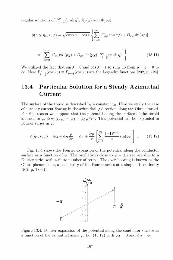
regular solutions of P qp− 1

2

(cosh η), Xp(χ) and Φq(ϕ):

φ(η ≤ η0, χ, ϕ) =√

cosh η − cosχ

∞∑

q=0

[Cqϕ cos(qϕ) +Dqϕ sin(qϕ)]

×[ ∞∑

p=0

[Cpχ cos(pχ) +Dpχ sin(pχ)]P qp− 1

2

(cosh η)

]

. (13.11)

We utilized the fact that sin 0 = 0 and cos 0 = 1 to sum up from p = q = 0 to∞. Here P 0

p− 1

2

(cosh η) ≡ Pp− 1

2

(cosh η) are the Legendre functions [202, p. 724].

13.4 Particular Solution for a Steady Azimuthal

Current

The surface of the toroid is described by a constant η0. Here we study the caseof a steady current flowing in the azimuthal ϕ direction along the Ohmic toroid.For this reason we suppose that the potential along the surface of the toroidis linear in ϕ, φ(η0, χ, ϕ) = φA + φBϕ/2π. This potential can be expanded inFourier series in ϕ:

φ(η0, χ, ϕ) = φA + φBϕ

2π= φA +

φBπ

[ ∞∑

q=1

(−1)q−1

qsin(qϕ)

]

. (13.12)

Fig. 13.4 shows the Fourier expansion of the potential along the conductorsurface as a function of ϕ. The oscillations close to ϕ = ±π rad are due to aFourier series with a finite number of terms. The overshooting is known as theGibbs phenomenon, a peculiarity of the Fourier series at a simple discontinuity[202, p. 783–7].

Figure 13.4: Fourier expansion of the potential along the conductor surface asa function of the azimuthal angle ϕ, Eq. (13.12) with φA = 0 and φB = φ0.

167

We assume that the potential inside the full solid toroidal Ohmic conductor(that is, for η > η0), Fig. 13.2a, is also given by Eq. (13.12), namely:

φ(η > η0, χ, ϕ) = φA + φBϕ

2π. (13.13)

The electric field inside the solid toroid can be expressed in cylindrical coordi-nates (ρ, ϕ, z) simply as:

~E = −∇φ = − φB2πρ

ϕ . (13.14)

This electric field does not lead to any accumulation of charges inside a full solidconductor because ∇ · ~E = 0.

These are reasonable results. The potential satisfies Laplace’s equation∇2φ = 0, as expected. The electric field is inversely proportional to the distanceρ =

√

x2 + y2 from the z axis. This was to be expected as we are assuminga conductor of uniform resistivity. The difference of potential ∆φ created bythe battery at ϕ = π rad can be related to the azimuthal electric field by a lineintegral:

∆φ = −∫ −π

ϕ=π

~E · d~ℓ = −Eϕ2πρ . (13.15)

Here ρ is the radius of a circular path centered on the z axis and located insideor along the surface of the toroid. This shows that Eϕ should be inverselyproportional to ρ, as found in Eq. (13.14). Comparing Eqs. (13.14) and (13.15)yields:

∆φ = φB . (13.16)

By Ohm’s law ~J = g ~E (where g is the uniform conductivity of the wire) we

can see that ~J is also inversely proportional to the distance ρ from the z axisinside a full solid homogeneous toroidal conductor.

We now consider the solution outside the conductor, valid for the cases of asolid and a hollow toroid.

We calculate Eq. (13.11) with η = η0 and utilize Eq. (13.12) as a boundarycondition of this problem. As we do not have terms with cos(qϕ) in Eq. (13.12),this means that Cqϕ = 0 for q = 1, 2, 3, . . . Comparing Eq. (13.11) at η = η0with Eq. (13.12) yields two equations connecting φA and φB to the C’s and D’s,namely:

φA = C0ϕ

√

cosh η0 − cosχ

∞∑

p=0

[Cpχ cos(pχ)

+ Dpχ sin(pχ)]Pp− 1

2

(cosh η0)

, (13.17)

φB =πqDqϕ

(−1)q−1

√

cosh η0 − cosχ

∞∑

p=0

[Cpχ cos(pχ)

168

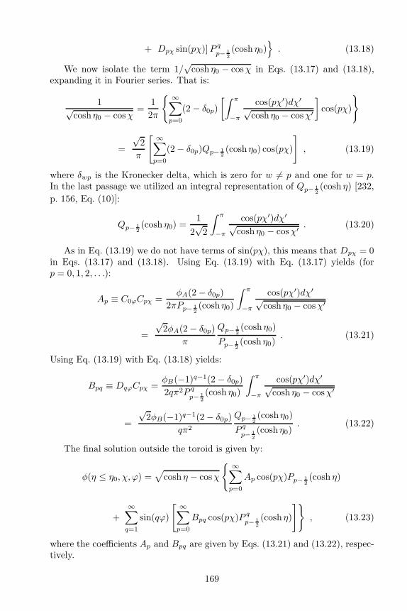
+ Dpχ sin(pχ)]P qp− 1

2

(cosh η0)

. (13.18)

We now isolate the term 1/√

cosh η0 − cosχ in Eqs. (13.17) and (13.18),expanding it in Fourier series. That is:

1√cosh η0 − cosχ

=1

2π

∞∑

p=0

(2 − δ0p)

[∫ π

−π

cos(pχ′)dχ′√

cosh η0 − cosχ′

]

cos(pχ)

=

√2

π

[ ∞∑

p=0

(2 − δ0p)Qp− 1

2

(cosh η0) cos(pχ)

]

, (13.19)

where δwp is the Kronecker delta, which is zero for w 6= p and one for w = p.In the last passage we utilized an integral representation of Qp− 1

2

(cosh η) [232,

p. 156, Eq. (10)]:

Qp− 1

2

(cosh η0) =1

2√

2

∫ π

−π

cos(pχ′)dχ′√

cosh η0 − cosχ′ . (13.20)

As in Eq. (13.19) we do not have terms of sin(pχ), this means that Dpχ = 0in Eqs. (13.17) and (13.18). Using Eq. (13.19) with Eq. (13.17) yields (forp = 0, 1, 2, . . .):

Ap ≡ C0ϕCpχ =φA(2 − δ0p)

2πPp− 1

2

(cosh η0)

∫ π

−π

cos(pχ′)dχ′√

cosh η0 − cosχ′

=

√2φA(2 − δ0p)

π

Qp− 1

2

(cosh η0)

Pp− 1

2

(cosh η0). (13.21)

Using Eq. (13.19) with Eq. (13.18) yields:

Bpq ≡ DqϕCpχ =φB(−1)q−1(2 − δ0p)

2qπ2P qp− 1

2

(cosh η0)

∫ π

−π

cos(pχ′)dχ′√

cosh η0 − cosχ′

=

√2φB(−1)q−1(2 − δ0p)

qπ2

Qp− 1

2

(cosh η0)

P qp− 1

2

(cosh η0). (13.22)

The final solution outside the toroid is given by:

φ(η ≤ η0, χ, ϕ) =√

cosh η − cosχ

∞∑

p=0

Ap cos(pχ)Pp− 1

2

(cosh η)

+

∞∑

q=1

sin(qϕ)

[ ∞∑

p=0

Bpq cos(pχ)P qp− 1

2

(cosh η)

]

, (13.23)

where the coefficients Ap and Bpq are given by Eqs. (13.21) and (13.22), respec-tively.

169

For the region inside the hollow toroid (that is, η > η0), Fig. 13.2b, wehave P q

p− 1

2

(cosh η → ∞) → ∞, while Qqp− 1

2

(cosh η → ∞) → 0. For this reason

we eliminate P qp− 1

2

(cosh η) as physical solutions for the region inside the hollow

toroid. The potential is then given by:

φ(η > η0, χ, ϕ) = φA +√

cosh η − cosχ

× ∞∑

q=1

sin(qϕ)

[ ∞∑

p=0

B′pq cos(pχ)Qq

p− 1

2

(cosh η)

]

, (13.24)

where the coefficients B′pq are defined by:

B′pq ≡

φB(−1)q−1(2 − δ0p)

2qπ2Qqp− 1

2

(cosh η0)

∫ π

−π

cos(pχ′)dχ′√

cosh η0 − cosχ′

=

√2φB(−1)q−1(2 − δ0p)

qπ2

Qp− 1

2

(cosh η0)

Qqp− 1

2

(cosh η0). (13.25)

Note that the potential inside the solid toroid, Eq. (13.13), and the potentialinside the hollow toroid, Eq. (13.24), are different. This happens because thediscontinuous boundary condition, Eq. (13.12), applies for any η > η0 insidethe solid toroid, particularly for ϕ→ π rad (φ→ φA + φB/2) and ϕ→ −π rad(φ → φA − φB/2), where the disc battery is located. See Fig. 13.2a. This doesnot happen to the hollow toroid, where the battery is a circumference, and thepotential must be continuous inside the hollow toroid. See Fig. 13.2b.

We plotted the equipotentials of a full solid toroid on the plane z = 0 inFig. 13.5 with φA = 0 and φB = φ0. We utilized a toroidal surface described byη0 = 2.187.

Figure 13.6 shows a plot of the equipotentials of the full solid toroid in theplane x = 0 (perpendicular to the current), also with φA = 0, φB = φ0, R0 = 1and η0 = 2.187.

13.5 Potential in Particular Cases

We now analyze the potential outside the toroid, Eq. (13.23), in four regions:(A) far away from the toroid, (B) close to the origin, (C) along the z axis, and(D) along the circumference described by x2 + y2 = a2 in the plane z = 0.

(A) For great distances from the toroid (that is, r =√

x2 + y2 + z2 ≫ a),Eqs. (13.2) to (13.5) yield:

η ≈ 2a√

x2 + y2

r2≪ 1 , (13.26)

cosh η ≈ 1 +2a2(x2 + y2)

r4→ 1 , (13.27)

170

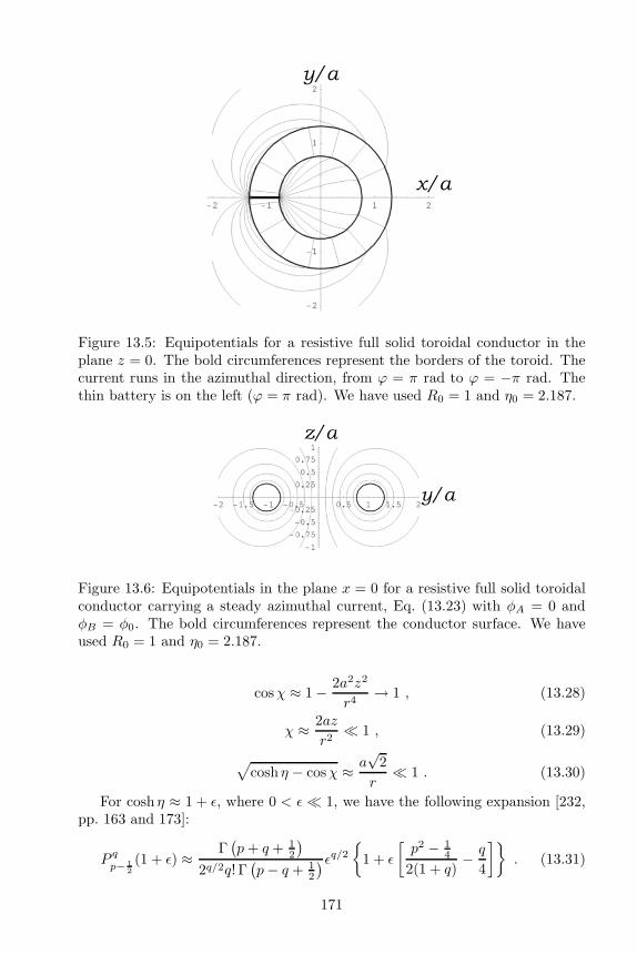
Figure 13.5: Equipotentials for a resistive full solid toroidal conductor in theplane z = 0. The bold circumferences represent the borders of the toroid. Thecurrent runs in the azimuthal direction, from ϕ = π rad to ϕ = −π rad. Thethin battery is on the left (ϕ = π rad). We have used R0 = 1 and η0 = 2.187.

Figure 13.6: Equipotentials in the plane x = 0 for a resistive full solid toroidalconductor carrying a steady azimuthal current, Eq. (13.23) with φA = 0 andφB = φ0. The bold circumferences represent the conductor surface. We haveused R0 = 1 and η0 = 2.187.

cosχ ≈ 1 − 2a2z2

r4→ 1 , (13.28)

χ ≈ 2az

r2≪ 1 , (13.29)

√

cosh η − cosχ ≈ a√

2

r≪ 1 . (13.30)

For cosh η ≈ 1 + ǫ, where 0 < ǫ ≪ 1, we have the following expansion [232,pp. 163 and 173]:

P qp− 1

2

(1 + ǫ) ≈ Γ(

p+ q + 12

)

2q/2q! Γ(

p− q + 12

)ǫq/2

1 + ǫ

[

p2 − 14

2(1 + q)− q

4

]

. (13.31)

171

That is, for q = 0 and for q = 1, 2, 3, ... we have, respectively:

Pp− 1

2

(1 + ǫ) ≈ 1 + ǫ

(

p2

2− 1

8

)

→ 1 , (13.32)

P qp− 1

2

(1 + ǫ) ≈ 2−q/2Γ(p+ q + 12 )

q!Γ(p− q + 12 )

ǫq/2 ≪ 1 . (13.33)

This means that the terms which appear in the potential for η ≪ 1, up tothe order ǫ1/2, are those which have the polynomials with q = 0 and with q = 1.That is, Pp− 1

2

(cosh η ≈ 1 + ǫ) ≈ 1 and P 1p− 1

2

(cosh η ≈ 1 + ǫ) ≈ (p2 − 1/4)√

ǫ/2.

The potential φ, Eq. (13.23), at great distances from the origin, is given inspherical coordinates (r, θ, ϕ) by (where ǫ = 2a2 sin2 θ/r2):

φ(r ≫ a, θ, ϕ) ≈ a√

2

r

∞∑

p=0

cos

(

p2a cos θ

r

)

×[

Ap +Bp1

(

p2 − 1

4

)

a

rsinϕ sin θ

]

, (13.34)

so that φ(r → ∞) → 0, as expected.(B) The potential close to the origin (that is, r ≪ a) can be calculated in

the same manner. In this approximation:

η ≈ 2√

x2 + y2

a≪ 1 , (13.35)

cosh η ≈ 1 +2(x2 + y2)

a2→ 1 , (13.36)

cosχ ≈ −1 +2z2

a2→ −1 , (13.37)

χ ≈ π − 2z

a→ π , (13.38)

√

cosh η − cosχ ≈√

2 +x2 + y2 − z2

√2a2

→√

2 . (13.39)

The potential (13.23) can be expressed as (with ǫ = 2r2 sin2 θ/a2):

φ(r ≪ a, θ, ϕ) ≈√

2

∞∑

p=0

(−1)p cos

(

p2r cos θ

a

)

×[

Ap +Bp1

(

p2 − 1

4

)

r

asinϕ sin θ

]

. (13.40)

(C) Along the z axis we have√

x2 + y2 = 0. From Eqs. (13.2) to (13.5) wehave:

η = 0 , (13.41)

172

cosh η = 1 , (13.42)

cosχ =z2 − a2

z2 + a2, (13.43)

√

cosh η − cosχ = a

√

2

z2 + a2. (13.44)

The potential (13.23) along the z axis can be written as:

φ(

r =√

x2 + y2 + z2 = |z|, θ, ϕ)

= a

√

2

z2 + a2

[ ∞∑

p=0

Ap cos

(

p arccosz2 − a2

z2 + a2

)

]

. (13.45)

(D) In the circumference described by x2 + y2 = a2, along the plane z =0, we have η → ∞. The associated Legengre functions P q

p− 1

2

(cosh η) and

Qqp− 1

2

(cosh η), for η ≫ 1 (and, therefore, for cosh η ≫ 1), can be approximated

utilizing [232, p. 164]:

Qqp− 1

2

(cosh η ≫ 1) ≈ (−1)q√πΓ(

p+ q + 12

)

2p+1

2 p! coshp+1

2 η, for any p , (13.46)

P qp− 1

2

(cosh η ≫ 1) ≈ 2p−1

2 (p− 1)! coshp−1

2 η√πΓ(

p− q + 12

) , for p > 0 , (13.47)

where Γ is the gamma function [202, p. 591]. The potential inside the hollowtoroid, Eq. (13.24), assumes the following form along this circumference:

φ(η → ∞, χ, ϕ) = φA − φBπ3/2

Q− 1

2

(cosh η0)

[ ∞∑

q=1

sin(qϕ)Γ(

q + 12

)

qQq− 1

2

(cosh η0)

]

. (13.48)

13.6 Electric Field and Surface Charges

In toroidal coordinates the gradient is written as:

∇φ =1

a(cosh η − cosχ)

(

η∂φ

∂η+ χ

∂φ

∂χ+

ϕ

sinh η

∂φ

∂ϕ

)

. (13.49)

The electric field can then be calculated by ~E = −∇φ, whose componentsfor the region outside the toroid (η < η0) are given by:

Eη = − sinh η√

cosh η − cosχ

a

∞∑

p=0

cos(pχ)

Ap

[

1

2Pp− 1

2

(cosh η)

173

+ (cosh η − cosχ)Pp− 1

2

′(cosh η)]

+

∞∑

q=1

sin(qϕ)Bpq

[

1

2P qp− 1

2

(cosh η) + (cosh η − cosχ)P qp− 1

2

′(cosh η)

]

,

(13.50)

Eχ = −√

cosh η − cosχ

a

∞∑

p=0

[

sinχ cos(pχ)

2− p(cosh η − cosχ) sin(pχ)

]

×[

ApPp− 1

2

(cosh η) +∞∑

q=1

sin(qϕ)BpqPq

p− 1

2

(cosh η)

]

, (13.51)

Eϕ = − (cosh η − cosχ)3/2

a sinh η

∞∑

q=1

q cos(qϕ)

[ ∞∑

p=0

Bpq cos(pχ)P qp− 1

2

(cosh η)

]

,

(13.52)where P q

p− 1

2

′(cosh η) are the derivatives of the P qp− 1

2

(cosh η) relative to cosh η.

The electric field inside the full solid toroid (η > η0) is given simply by:

Eη = 0 , Eχ = 0 , Eϕ = −coshη − cosχ

a sinh η

φB2π

= − φB

2π√

x2 + y2.

(13.53)The total surface charge distribution σt that creates the electric field inside

(and outside of) the conductor, keeping the current flowing, can be obtainedwith Gauss’s law (by choosing a Gaussian surface involving a small portion ofthe conductor surface) for the full solid toroid, Fig. 13.2a:

σt(η0, χ, ϕ) = ε0

[

~E(η < η0) · (−η) + ~E(η > η0) · η]

η0

=ε0 sinh η0

a

φA + φBϕ/2π

2+ (cosh η0 − cosχ)3/2

× ∞∑

p=0

cos(pχ)[

ApPp− 1

2

′(cosh η0) +

∞∑

q=1

sin(qϕ)BpqPq

p− 1

2

′(cosh η0)]

.

(13.54)

13.7 Thin Toroid Approximation

Suppose that the toroid is very thin, with its radii described by a greater radiusR0 = a cosh η0/ sinh η0 ≈ a and smaller radius r0 = a/ sinh η0, such that r0 ≪

174

R0. See Fig. 13.1. The surface of the toroid is described by η0 ≫ 1 and,consequently, cosh η0 ≫ 1.

In this approximation, the potential inside the hollow toroid and inside thefull solid toroid is given by the same expression, Eq. (13.13). The electric fieldis given by Eqs. (13.14) and (13.53). This means that there is no distributionof surface charges in the internal surface of a hollow thin toroid.

The Legendre functions of the second kind calculated at η = η0, given byQp− 1

2

(cosh η0), appear in the coefficients Ap and Bpq of the potential outside

the toroid, Eqs. (13.21) and (13.22), respectively. As Eq. (13.46), calculated in

η = η0 and for q = 0, has a factor of cosh−p−1/2 η0 ≪ 1, we can neglect allterms in Eq. (13.23) having p > 0 compared with the term having p = 0. Thepotential outside the thin toroid (η0 ≫ 1) can then be written as:

φ(η ≤ η0, χ, ϕ) =

√

cosh η − cosχ

cosh η0

φAP− 1

2

(cosh η)

P− 1

2

(cosh η0)

+φBπ

[ ∞∑

q=1

(−1)q−1

qsin(qϕ)

P q− 1

2

(cosh η)

P q− 1

2

(cosh η0)

]

. (13.55)

It is interesting to find the expressions for the potential and electric fieldoutside but in the vicinity of the conductor (that is, η0 > η ≫ 1). A seriesexpansion of the functions P q− 1

2

(Υ) and P q− 1

2

′(Υ) around Υ → ∞ gives as the

most relevant terms [232, p. 173]:

P q− 1

2

(Υ) ≈√

2/π

Γ(1/2 − q)

ln(2Υ) − ψ(1/2 − q) − γ√Υ

, (13.56)

P q− 1

2

′(Υ) ≈√

2/π

Γ(1/2 − q)

1

Υ3/2

[

1 − ln(2Υ) − ψ(1/2 − q) − γ

2

]

, (13.57)

where ψ(z) = Γ′(z)/Γ(z) is the digamma function, and γ ≈ 0.577216 is theEuler gamma.

The potential just outside the thin toroid, Eq. (13.55), can then be writtenin this approximation as (utilizing that ψ(1/2) + γ = − ln 4):

φ(η0 ≥ η ≫ 1, χ, ϕ) = φAln(8 cosh η)

ln(8 coshη0)

+φBπ

[ ∞∑

q=1

(−1)q−1

qsin(qϕ)

ln(2 cosh η) − ψ(

12 − q

)

− γ

ln(2 cosh η0) − ψ(

12 − q

)

− γ

]

. (13.58)

This equation is valid for −π rad ≤ ϕ ≤ π rad, even close to the battery.

175

The electric field close to the surface of the thin toroid, just outside it,obtained from Eq. (13.58), is given by:

Eη = − sinh η

a

φAln(8 cosh η0)

+φBπ

[ ∞∑

q=1

(−1)q−1

q

sin(qϕ)

ln(2 cosh η0) − ψ(

12 − q

)

− γ

]

, (13.59)

Eχ = 0 , (13.60)

Eϕ = −φBπa

[ ∞∑

q=1

(−1)q−1 cos(qϕ)ln(2 cosh η) − ψ

(

12 − q

)

− γ

ln(2 cosh η0) − ψ(

12 − q

)

− γ

]

.(13.61)

Note that

Eϕ(η0) = −φBπa

[ ∞∑

q=1

(−1)q−1 cos(qϕ)

]

= − φB2πa

. (13.62)

That is, it coincides exactly with the electric field inside the solid toroid, Eq. (13.14).This is a divergent series presented in Eq. (11.30) which arises from differenti-ation of a convergent Fourier series, as we discussed in Section 11.4. It can behandled by the average procedure presented in Eq. (11.32).

The surface charge distribution in this thin toroid approximation is givenby, from Eq. (13.59):

σ(η0 ≫ 1, χ, ϕ) = −ε0Eη(η0) =ε0 sinh η0

a

[

φAln(8 cosh η0)

+φBπ

( ∞∑

q=1

(−1)q−1

q

sin(qϕ)

ln(2 coshη0) − ψ(

12 − q

)

− γ

)]

, (13.63)

which is also valid for −π rad ≤ ϕ ≤ π rad. As there is no surface chargedistribution in the internal surface of a hollow thin toroid, this expression meansthe total surface charge distribution which exists only in the external surface ofthe (hollow or solid) thin toroid.

In Fig. 13.7 we plotted the density of surface charges σ as a function of theazimuthal angle ϕ obtained from Eq. (13.63). We can see that σ is linear withϕ close to ϕ = 0 rad. Close to the battery σ diverges to infinity (that is, σ → ∞when ϕ → ±π rad). To our knowledge the first to conclude correctly that thesurface charge density in a resistive ring carrying a steady current grows towardthe battery as a function of the azimuthal angle ϕ in a pace faster than linearlywas Weber in 1852. See the Appendix A.

From Figure 13.7 and Eq. (11.11) we can then write the summation ofEq. (13.63) for a thin toroid and far from the battery (that is, for η0 ≫ 1and ϕ≪ π rad) as

176

Figure 13.7: Density of surface charges as a function of the azimuthal angle ϕobtained from Eq. (13.63) with φA = 0 and η0 = 10 (R0/r0 = 1.1 × 104). It islinear with ϕ when ϕ ≈ 0 rad but then diverges to infinity close to the battery.

∞∑

q=1

(−1)q−1

q

sin(qϕ)

ln(2 cosh η0) − ψ(

12 − q

)

− γ≡ g(η0)

ϕ

2. (13.64)

Here g(η0) is a dimensionless function of η0 defined by this equation.With this definition Eq. (13.63) can be written as

σ(η0 ≫ 1, χ, ϕ≪ π) ≈ ε0 sinh η0a

φAln(8 cosh η0)

+ε0 sinh η0

ag(η0)φB

ϕ

2π

≡ σA + σBϕ

2π. (13.65)

The constants σA and σB are defined by this equation, namely

σA ≡ ε0 sinh η0a

φAln(8 cosh η0)

, (13.66)

σB ≡ ε0 sinh η0a

g(η0)φB . (13.67)

Combining Eq. (13.67) with Eq. (13.62) we can write the tangential compo-nent of the electric field Eϕ at the surface of the thin toroid as

Eϕ(η0 ≫ 1) = − φB2πa

= − σB2πε0 sinh η0g(η0)

. (13.68)

As we will see in Appendix A, Weber was the first to obtain an analogousto this result. His approach of dealing with this problem leads to a tangentialcomponent of the electric field for a very thin toroid as given by Eq. (A.20),namely:

Eϕ(η0 ≫ 1) ≈ − r0σB2πε0R0

(

ln8R0

r0− π

2

)

. (13.69)

By comparing Eqs. (13.68) and (13.69) for a very thin toroid (η0 ≫ 1,a ≈ R0, sinh η0 = a/r0 ≈ R0/r0) we can then try to fit g(η0) as

177

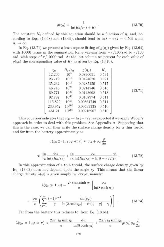
g(η0) ≡1

ln(R0/r0) +K0. (13.70)

The constant K0 defined by this equation should be a function of η0 and, ac-cording to Eqs. (13.68) and (13.69), should tend to ln 8 − π/2 = 0.509 whenη0 → ∞.

In Eq. (13.71) we present a least-square fitting of g(η0) given by Eq. (13.64)with 10000 terms in the summation, for ϕ varying from −π/100 rad to π/100rad, with steps of π/10000 rad. At the last column we present for each value ofg(η0) the corresponding value of K0 as given by Eq. (13.70).

η0 R0/r0 g(η0) K0

12.206 105 0.0830051 0.53423.719 1010 0.0424678 0.52135.232 1015 0.0285259 0.51746.745 1020 0.0214746 0.51569.771 1030 0.0143698 0.51392.797 1040 0.0107974 0.511115.822 1050 0.00864749 0.511230.952 10100 0.00433335 0.510461.21 10200 0.00216907 0.510

(13.71)

This equation indicates thatK0 → ln 8−π/2, as expected if we apply Weber’sapproach in order to deal with this problem. See Appendix A. Supposing thatthis is the case, we can then write the surface charge density for a thin toroidand far from the battery approximately as

σ(η0 ≫ 1, χ, ϕ≪ π) ≈ σA + σBϕ

2π

≈ ε0r0

φAln(8R0/r0)

+ε0r0

φBln(R0/r0) + ln 8 − π/2

ϕ

2π. (13.72)

In this approximation of a thin toroid, the surface charge density given byEq. (13.63) does not depend upon the angle χ. This means that the linearcharge density λ(ϕ) is given simply by 2πr0σ, namely:

λ(η0 ≫ 1, ϕ) =2πr0ε0 sinh η0

a

[

φAln(8 cosh η0)

+φBπ

( ∞∑

q=1

(−1)q−1

q

sin(qϕ)

ln(2 coshη0) − ψ(

12 − q

)

− γ

)]

. (13.73)

Far from the battery this reduces to, from Eq. (13.64):

λ(η0 ≫ 1, ϕ≪ π) ≈ 2πr0ε0 sinh η0a

φAln(8 cosh η0)

+2πr0ε0 sinh η0

ag(η0)φB

ϕ

2π

178

≡ λA + λBϕ

2π. (13.74)

The constants λA and λB were defined by this equation.We can calculate the total charge qA of the thin toroid as a function of the

constant electric potential φA. For this end, we integrate the surface chargedensity σ in χ and ϕ (in the approximation cosh η0 ≫ 1):

qA =

∫ π

−πhχdχ

∫ π

−πhϕdϕσ(χ, ϕ) =

4π2ε0φAR0

ln(8 coshη0)≈ 4π2ε0φAR0

ln(8R0/r0), (13.75)

where hη = hχ = a/(cosh η − cosχ) and hϕ = a sinh η/(cosh η − cosχ) are thescale factors in toroidal coordinates [233]. Notice that from Eq. (13.75) we canobtain the capacitance of the thin toroid [234, p. 127]:

C =qAφA

=4π2ε0R0

ln(8 cosh η0)=

4π2ε0R0

ln(8R0/r0). (13.76)

The potential along the z axis is given by, from Eq. (13.45) in the thin toroidapproximation:

φ(

r =√

x2 + y2 + z2 = |z|, θ, ϕ)

=qA

4πε0

1√z2 + a2

. (13.77)

Eq. (13.77) coincides with the coulombian result of a charged thin toroid ofradius a in the z = 0 plane and total charge qA.

As we have seen, in the case of a thin toroid the term in the potential withp = 0 is much larger than the terms with p > 0. This means that Eq. (13.34)reduces to

φ(r ≫ a, θ, ϕ) ≈ a√

2

r

[

A0 −B01

4

a

rsinϕ sin θ

]

. (13.78)

With Eqs. (13.21) and (13.22) we obtain

φ(r ≫ a, θ, ϕ) ≈ a√

2

r

[√2φAπ

Q− 1

2

(cosh η0)

P− 1

2

(cosh η0)

−√

2φBπ2

Q− 1

2

(cosh η0)

P 1− 1

2

(cosh η0)

a

4rsinϕ sin θ

]

. (13.79)

We now simplify the last two equations utilizing Eqs. (13.46), (13.56) andthe relations

Γ(1/2) =√π , Γ(−1/2) = −2

√π , (13.80)

ψ(1/2) + γ = − ln 4 , ψ(−1/2) + γ = 2 − ln 4 . (13.81)

179

This yields:

φ(r ≫ a, θ, ϕ) ≈ aπ

r

φAln(8 cosh η0)

+φB

2π[ln(8 cosh η0) − 2]

a

rsinϕ sin θ

.

(13.82)

Utilizing a similar procedure beginning with Eq. (13.40) yields:

φ(r ≪ a, θ, ϕ) ≈ π

φAln(8 cosh η0)

+φB

2π[ln(8 cosh η0) − 2]

r

asinϕ sin θ

.

(13.83)

13.8 Comparison of the Thin Toroid Carrying a

Steady Current with the Case of a Straight

Cylindrical Wire Carrying a Steady Cur-

rent

It is useful to define a new coordinate system:

s′ = aϕ , ρ′ =

√

(

√

x2 + y2 − a)2

+ z2 . (13.84)

We can interpret s′ as a distance along the toroid surface in the ϕ direction,and ρ′ as the shortest distance from the circumference x2 + y2 = a2 located inthe plane z = 0. When η0 > η ≫ 1 (that is, r0 < ρ′ ≪ a), Eqs. (13.84) and(13.4) result in cosh η ≈ a/ρ′ ≫ 1 and cosh η0 ≈ a/r0 ≫ 1. For η0 ≥ η ≫ 1 wecan approximate the term inside square brackets of Eq. (13.58) by (taking intoaccount Eq. (11.11)):

∞∑

q=1

(−1)q−1

qsin(qϕ)

ln(2 cosh η) − ψ(

12 − q

)

− γ

ln(2 cosh η0) − ψ(

12 − q

)

− γ

≈( ∞∑

q=1

(−1)q−1

qsin(qϕ)

)

ln(cosh η)

ln(cosh η0)=ϕ

2

ln(cosh η)

ln(cosh η0). (13.85)

Utilizing Eqs. (13.85) and (13.84) into Eq. (13.58) yields:

φ(η0 ≥ η ≫ 1, χ, ϕ) = φAln(8a/ρ′)

ln(8a/r0)+ φB

s′

2πa

ln(a/ρ′)

ln(a/r0). (13.86)

Eq. (13.86) can be written in a slightly different form. Consider a certainpiece of the toroid between the angles ϕ0 and −ϕ0, with potentials in these

180

extremities given by φR = φA+φBϕ0/2π and φL = φA−φBϕ0/2π, respectively.This piece has a length of ℓ = 2aϕ0. The potential can then be written as:

φ = φAln(ℓ/ρ′) − ln(ℓ/8a)

ln(ℓ/r0) − ln(ℓ/8a)+ φB

ϕ0s′

πℓ

ln(ℓ/ρ′) − ln(ℓ/a)

ln(ℓ/r0) − ln(ℓ/a)

≈[

φR + φL2

+ (φR − φL)s′

ℓ

]

ln(ℓ/ρ′)

ln(ℓ/r0). (13.87)

In the last approximation we neglected the terms ln(ℓ/8a) and ln(ℓ/a) in com-parison with the terms ln(ℓ/ρ′) and ln(ℓ/r0) utilizing the approximation r0 <ρ′ ≪ a (so that ℓ/r0 > ℓ/ρ′ ≫ ℓ/a). The electric field can be expressed in thisapproximation as:

~E = −[

φR + φL2

+ (φR − φL)s′

ℓ

]

η

ρ′ ln(ℓ/r0)− φR − φL

ℓ

ln(ℓ/ρ′)

ln(ℓ/r0)ϕ . (13.88)

Eqs. (13.87) and (13.88) can be compared to Eqs. (6.17) and (6.18), re-produced as Eqs. (13.89) and (13.90), respectively. These equations refer toa long straight cylindrical conductor of radius r0 carrying a constant current,in cylindrical coordinates (ρ′, ϕ, z) (note that the conversions from toroidal tocylindrical coordinates in this approximation are η ≈ −ρ′ and ϕ ≈ z). In thiscase, the cylinder has a length ℓ and radius r0 ≪ ℓ, with potentials φL and φRin the extremities of the conductor, and RI = φL − φR:

φ(r ≥ a) =

[

φR + φL2

+ (φR − φL)z

ℓ

]

ln(ℓ/ρ′)

ln(ℓ/r0), (13.89)

~E(ρ′ ≥ a) =

[

φR + φL2

+ (φR − φL)z

ℓ

]

ρ′

ρ′ ln(ℓ/r0)− φR − φL

ℓ

ln(ℓ/ρ′)

ln(ℓ/r0)z .

(13.90)The potential in the region close to the thin toroid coincides with the cylin-

drical solution, as expected.

13.9 Charged Toroid without Current

Consider a toroid described by η0, without current but charged to a constantpotential φA. Using φB = 0 in Eqs. (13.23), (13.13) and (13.24) we have thepotential inside and outside the toroid, respectively:

φ(η ≥ η0, χ, ϕ) = φA , (13.91)

φ(η ≤ η0, χ, ϕ) =√

cosh η − cosχ

[ ∞∑

p=0

Ap cos(pχ)Pp− 1

2

(cosh η)

]

, (13.92)

181

where Pp− 1

2

(cosh η0) are the Legendre functions, and the coefficients Ap are

given by Eq. (13.21). This solution is already known in the literature [235,p. 239] [236, p. 1304].

It is also possible to obtain the capacitance of the toroid. To this end we com-pare the electrostatic potential at a distance r far from the origin, Eq. (13.34),with the potential given by a point charge q, φ(r ≫ a) ≈ q/4πε0r:

φ(r ≫ a, θ, ϕ) ≈ a√

2

r

[ ∞∑

p=0

√2φA(2 − δ0p)

π

Qp− 1

2

(cosh η0)

Pp− 1

2

(cosh η0)

]

=q

4πε0r. (13.93)

The capacitance of the toroid with its surface at a constant potential φA canbe written as C = q/φA. From Eq. (13.93) this yields [235, p. 239] [237, p. 5-13][238, p. 9] [239, p. 375]:

C = 8ε0a

[ ∞∑

p=0

(2 − δ0p)Qp− 1

2

(cosh η0)

Pp− 1

2

(cosh η0)

]

. (13.94)

Utilizing the thin toroid approximation, η0 ≫ 1, one can obtain the capacitanceof a circular ring, Eq. (13.76).

Another case of interest is that of a charged circular wire already discussed,which is the particular case of a toroid with r0 → 0. In this case the chargedtoroid reduces to an uniformly charged circumference of radius R0 = a. Withη0 ≫ 1 and cosh η0 ≫ 1 we have R0 ≈ a. Keeping only the term with p = 0 inEqs. (13.21) and (13.92) yields (with Eq. (13.75)):

φ(η ≤ η0, χ, ϕ) = φA

√

cosh η − cosχ

cosh η0

P− 1

2

(cosh η)

P− 1

2

(cosh η0)

=qA

4π√

2ε0a

√

cosh η − cosχP− 1

2

(cosh η) . (13.95)

Expressed in spherical coordinates (r, θ, ϕ), the potential for the thin toroidbecomes:

φ(r, θ, ϕ) =qA

4πε0

1

[(r2 − a2)2 + 4a2r2 cos2 θ]1/4

×P− 1

2

(

r2 + a2

√

(r2 − a2)2 + 4a2r2 cos2 θ

)

. (13.96)

From Eqs. (13.91) and (13.75) we can see that the constant electrostaticpotential along the thin toroid expressed in terms of its total charge qA is givenby:

φ(r0 ≪ R0, θ, ϕ) =qA/2πa

2πε0ln

8a

r0. (13.97)

Even when the linear charge density qA/2πa remains constant, we can see fromthis expression that the potential diverges logarithmically when a/r0 → ∞.

182

We can expand Eq. (13.96) in powers of r</r>, where r< (r>) is the lesser

(greater) of a and r =√

x2 + y2 + z2. We present the first three terms:

φ(r, θ, ϕ) ≈ qA4πε0

1

r>− 1 + 3 cos(2θ)

8

r2<r3>

+3

512

[

9 + 20 cos(2θ) + 35 cos(4θ)]r4<r5>

. (13.98)

Eqs. (13.95) to (13.98) can be compared with the solution given by Jackson[13, p. 104]. Jackson gives the exact electrostatic solution of the problem ofa charged circular wire (that is, a toroid with radius r0 = 0), in sphericalcoordinates (r, θ, ϕ):

φ(r, θ, ϕ) =qA

4πε0

[ ∞∑

n=0

r2n<r2n+1>

(−1)n(2n− 1)!!

2nn!P2n(cos θ)

]

, (13.99)

where qA is the total charge of the wire. Eq. (13.99) expanded to n = 2 yieldsexactly Eq. (13.98). We have checked that Eqs. (13.96) and (13.99) are the samefor at least n = 30.

We plotted both Eqs. (13.95) and (13.99), in Fig. 13.8. They yield the sameresult, as expected. It is worthwhile to note that in spherical coordinates wehave an infinite sum, Eq. (13.99), while in toroidal coordinates the solution isgiven by a single term, Eq. (13.95). The agreement shows that Eqs. (13.95) and(13.99) are the same solution only expressed in different forms.

Figure 13.8: Equipotential lines on the plane x = 0 (perpendicular to the toroid)for the charged thin wire without current. Both Eqs. (13.95) and (13.99) coincidewith one another. We utilized η0 = 38 (cosh η0 = 1.6× 1016) and a = 1. Noticethe difference between this Figure and Figure 13.6: the left and right sides ofthe conductor here possess the same charge signs, while in Figure 13.6 they haveopposite signs.

Fig. 13.9 shows the potential as function of ρ (in cylindrical coordinates) inthe plane z = 0. Eqs. (13.95) and (13.99) give the same result.

183

Figure 13.9: Normalized potential as a function of ρ (distance to the z axis)on the plane z = 0. Eqs. (13.95) and (13.99) give the same result. We utilizedη0 = 38 (cosh η0 = 1.6 × 1016) and a = 1.

Along the z axis, i.e., for√

x2 + y2 = 0, the potential represented byEq. (13.96) is given by:

φ(r, θ, ϕ) =qA

4πε0

1√z2 + a2

. (13.100)

This is the same result which arises from a direct integration of the electro-static potential. That is, a charge qA uniformly distributed along a filiformring of radius a, located at the plane z = 0 and centered along the z axis [202,Example 12.3.3].

13.10 Comparison with Experimental Results

Figure 13.5 can be compared with the experimental result found by Jefimenko[174, Fig. 3], reproduced here in Fig. 13.10 with Fig. 13.5 overlaid on it. Theequipotential lines obtained here are orthogonal to the electric field lines. Thereis a very reasonable agreement between the theoretical result and the experi-ment.

In order to have a better fit to his data we should consider an extendedbattery. As we can see from his account of the experiment, Jefimenko paintedtwo sections of his strip with a conducting ink of much smaller resistivity thanthe remainder of the strip. These sections located at −ϕj < ϕ < −ϕi andϕi < ϕ < ϕj were charged to opposite potentials. Considering these sections asof zero resistivity we can model analytically the potential inside and along thesurface of the toroid as:

φ(η ≥ η0, χ, ϕ) =

−φB ϕi

2ππ+ϕπ−ϕj

, −π < ϕ < −ϕj ,−φBϕi/2π, −ϕj < ϕ < −ϕi ,φBϕ/2π, −ϕi < ϕ < ϕi ,φBϕi/2π, ϕi < ϕ < ϕj ,φB

ϕi

2ππ−ϕπ−ϕj

, ϕj < ϕ < π .

(13.101)

184

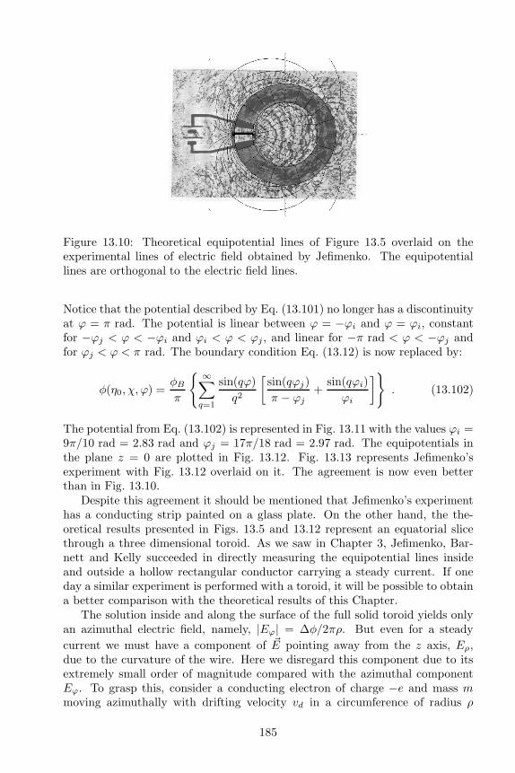
Figure 13.10: Theoretical equipotential lines of Figure 13.5 overlaid on theexperimental lines of electric field obtained by Jefimenko. The equipotentiallines are orthogonal to the electric field lines.

Notice that the potential described by Eq. (13.101) no longer has a discontinuityat ϕ = π rad. The potential is linear between ϕ = −ϕi and ϕ = ϕi, constantfor −ϕj < ϕ < −ϕi and ϕi < ϕ < ϕj , and linear for −π rad < ϕ < −ϕj andfor ϕj < ϕ < π rad. The boundary condition Eq. (13.12) is now replaced by:

φ(η0, χ, ϕ) =φBπ

∞∑

q=1

sin(qϕ)

q2

[

sin(qϕj)

π − ϕj+

sin(qϕi)

ϕi

]

. (13.102)

The potential from Eq. (13.102) is represented in Fig. 13.11 with the values ϕi =9π/10 rad = 2.83 rad and ϕj = 17π/18 rad = 2.97 rad. The equipotentials inthe plane z = 0 are plotted in Fig. 13.12. Fig. 13.13 represents Jefimenko’sexperiment with Fig. 13.12 overlaid on it. The agreement is now even betterthan in Fig. 13.10.

Despite this agreement it should be mentioned that Jefimenko’s experimenthas a conducting strip painted on a glass plate. On the other hand, the the-oretical results presented in Figs. 13.5 and 13.12 represent an equatorial slicethrough a three dimensional toroid. As we saw in Chapter 3, Jefimenko, Bar-nett and Kelly succeeded in directly measuring the equipotential lines insideand outside a hollow rectangular conductor carrying a steady current. If oneday a similar experiment is performed with a toroid, it will be possible to obtaina better comparison with the theoretical results of this Chapter.

The solution inside and along the surface of the full solid toroid yields onlyan azimuthal electric field, namely, |Eϕ| = ∆φ/2πρ. But even for a steady

current we must have a component of ~E pointing away from the z axis, Eρ,due to the curvature of the wire. Here we disregard this component due to itsextremely small order of magnitude compared with the azimuthal componentEϕ. To grasp this, consider a conducting electron of charge −e and mass mmoving azimuthally with drifting velocity vd in a circumference of radius ρ

185

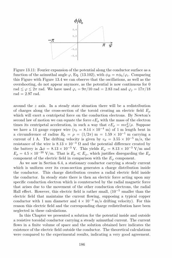
Figure 13.11: Fourier expansion of the potential along the conductor surface as afunction of the azimuthal angle ϕ, Eq. (13.102), with φB = πφ0/ϕi. Comparingthis Figure with Figure 13.4 we can observe that the oscillations, as well as theovershooting, do not appear anymore, as the potential is now continuous for 0rad ≤ ϕ ≤ 2π rad. We have used ϕi = 9π/10 rad = 2.83 rad and ϕj = 17π/18rad = 2.97 rad.

around the z axis. In a steady state situation there will be a redistributionof charges along the cross-section of the toroid creating an electric field Eρwhich will exert a centripetal force on the conduction electrons. By Newton’ssecond law of motion we can equate the force eEρ with the mass of the electrontimes its centripetal acceleration, in such a way that eEρ = mv2

d/ρ. Supposewe have a 14 gauge copper wire (r0 = 8.14 × 10−4 m) of 1 m length bent ina circumference of radius R0 = ρ = (1/2π) m = 1.59 × 10−1 m carrying acurrent of 1 A. The drifting velocity is given by vd = 3.55 × 10−5 m/s, theresistance of the wire is 8.13 × 10−3 Ω and the potential difference created bythe battery is ∆φ = 8.13 × 10−3 V. This yields Eϕ = 8.13 × 10−3 V/m andEρ = 4.5 × 10−20 V/m. That is Eρ ≪ Eϕ, which justifies disregarding the Eρcomponent of the electric field in comparison with the Eϕ component.

As we saw in Section 6.4, a stationary conductor carrying a steady currentwhich is uniform over its cross-section generates a charge distribution insidethe conductor. This charge distribution creates a radial electric field insidethe conductor. In steady state there is then an electric force acting upon anyspecific conduction electron which is counteracted by the radial magnetic forcethat arises due to the movement of the other conduction electrons, the radialHall effect. However, this electric field is rather small, (10−5 smaller than theelectric field that maintains the current flowing, supposing a typical copperconductor with 1 mm diameter and 4 × 10−3 m/s drifting velocity). For thisreason this electric field and the corresponding charge redistribution have beenneglected in these calculations.

In this Chapter we presented a solution for the potential inside and outsidea resistive toroidal conductor carrying a steady azimuthal current. The currentflows in a finite volume of space and the solution obtained here indicates theexistence of the electric field outside the conductor. The theoretical calculationswere compared to the experimental results, indicating a very good agreement.

186

Figure 13.12: Equipotentials in the plane z = 0 for a resistive toroidal conductorcarrying a steady azimuthal current, using Eq. (13.102) as boundary conditionand φB = πφ0/ϕi. The bold circumferences represent the conductor surfaceand the bold straight lines represent the angles ϕ = ±ϕi = ±9π/10 rad = 2.83rad and ϕ = ±ϕj = ±17π/18 rad = 2.97 rad. We have used η0 = 2.187.

Figure 13.13: Jefimenko’s experiment with Figure 13.12 overlaid on it – theequipotential lines are orthogonal to the electric field lines.

187

We also obtained the distribution of charges along the surface of the resistivering carrying a steady current, a subject which was first considered by WilhelmWeber 150 years ago, as we see in the Appendix. Weber made the first pre-liminary quantitative calculations related to this problem, and this specific casehas essentially been forgotten these many years. This Chapter can be seen as afulfillment of one of Weber’s goals. That is, to derive the distribution of surfacecharges in a ring which, together with the battery, creates a constant tangentialelectric field for all azimuthal angles inside the ring. We have also succeeded inderiving the force exerted upon a stationary and external point charge by thisstationary ring carrying a steady current.

188

Part IV

Open Questions

189

Chapter 14

Future Prospects

In this book we presented the main simple cases which can be treated analyt-ically. The goal now might be to consider theoretically other situations whichhave already been analyzed experimentally. Examples include the current flow-ing in a disc, Figure 3.7; current-carrying wedges with the two halves connectedin parallel and in series, Figure 3.6; etc. The latter situation is interesting inorder to know quantitatively the correct distribution of charges allowing thecurrent to bend around a corner. Studies along these lines include Rosser [167],Jefimenko [240] [176, pp. 302-303] and the book by Chabay and Sherwood [165,Chapter 6].

Other interesting aspects are connected with the distribution of surfacecharges close to the battery and inside it. In Chapters 11 to 13 we discussed thisin the cases of a cylindrical shell, a spherical shell and a ring with azimuthalcurrents. Another important discussion for the case of a coaxial cable of fi-nite size has been given by Jackson [12]. Saslow considered a spherical batterysurrounded by a conducting medium and analyzed the distribution of chargesupon the surface of the battery [241]. The distribution of surface charges closeto a battery in the case of straight conductors carrying steady currents hasbeen treated for two different configurations in 2004 [205] and 2005 [222]. Othercases should also be studied quantitatively in different configurations. Althoughit might be difficult to obtain detailed information analytically about the distri-bution of surface charges in a battery of finite size, this might be accomplishedwith computer calculations and numerical plots.

It would also be important to analyze cases in which the current is notgenerated by a chemical battery, but by the relative motion between a closedconducting circuit and a magnet, as in the first case considered qualitativelyby Weber and described in the Appendix. Calculations have been performedrelative to the surface charges in the case of a square circuit in the presence of avariable magnetic flux [242], and also the case of a ring rotating in the presenceof a magnetic field [243]. It would be important to extend the calculations toother spatial configurations and analogous situations.

Another situation which has received little attention up to now is the dis-

191

tribution of charges in resistive conductors carrying steady currents when theseconductors are composed of two or more different materials. That is, the chargesthat accumulate on the interface between a conductor and a resistor, or on theinterface of two conductors with different resistivities. Some authors who haveconsidered this problem include Jefimenko [240], Heald [226], Hartel [244, 245],Chabay and Sherwood [165, 166], and Jackson [12]. Jackson’s work has an in-teresting comparison of the distribution of surface charges in a circuit with alarge resistance and in an equivalent open circuit, i.e., with the resistor removedfrom the circuit.

Another relevant topic is to consider in detail the behavior of surface chargesand the corresponding external electric field in the transition from steady-currents to low and high frequency circuits with alternating currents. Importantdiscussions of this subject have been given by Jackson [12] and Preyer [246]. We-ber and Kirchhoff’s works related with the telegraphy equation discussed in theAppendices should also be reconsidered and extended to different cases andconfigurations [30, 31].

Beyond these future extensions, there are a number of topics which stillneed to be clarified. Consider a stationary point charge close to a stationarypermanent magnet. Is there a net force between them beyond the force due toelectrostatic origin? That is, is there a force depending upon the magnetizationof the magnet, or depending upon the magnetic field it produces? As we haveseen in this book, there is a force between a stationary point charge and astationary resistive circuit carrying a steady current. This force is proportionalto the electromotive force of the battery. Is there a similar force between astationary magnet and a stationary external charge? In this question we arenot including the force due to electrostatic induction which must exist betweena conducting magnet and the external charge, which is of electrostatic origin(due to image charges, etc.) The magnet we are considering here has permanentmagnetization. Its magnetic field is due to permanent microscopic or molecularcurrents in its interior. The magnet is not connected to a chemical battery andfor this reason it should not have a distribution of surface charges as in the caseof a resistive wire carrying a steady current. In any event this subject shouldbe better analyzed and careful experiments should be performed to answer thisquestion.

Analogously, there should not exist an electric field outside a wire made ofa superconducting material if it carries a steady current without any externalsource of electromotive force, i.e., if there is no battery connected to the wire.As this wire has no resistance and is not connected to any battery, there shouldbe no electric field outside the wire (except for the zeroth order electric field ifwe approach a test charge to the wire). But it should be emphasized once morethat only experiments can decide this question.

A possible connection between the external electric field around a resistivecylindrical conductor carrying a steady current and the Aharonov-Bohm effectwas discussed in 2001 [247]. Although this idealized infinite conductor willnot produce any external magnetic field, it will produce an external electricfield if the solenoid is connected to a chemical battery. This electric field is

192

not considered by most authors, as they are unaware of its existence. For thisreason none of them considered the influence of this steady electric field in theAharonov-Bohm effect, taking into account only the magnetic vector potential.The goal of our paper was to call attention to this external electric field for theanalysis of the Aharonov-Bohm effect.

In this book we have shown that a force must exist between a point chargeand a resistive wire carrying a steady current when they are at rest relative toone another. It has been shown theoretically that this force (or the electric fieldoutside the wire) is proportional to the emf of the battery. But it is still necessaryto show experimentally the proportionality between this force and the voltageof the battery. This proportionality should appear according to the calculationspresented here. They have yielded qualitative agreement with the experimentsof Bergmann, Schaefer, Jefimenko, Barnett and Kelly relating to equipotentialsand electric field lines. But we are not not aware of any experiment showingdirectly the proportionality between this force and the voltage generated by thebattery.

Another crucial question which still needs to be settled empirically is relatedto the second order electric field (proportional to the square of the current, orto the square of the drifting velocity of the mobile electrons). Alternatively wemight ask if there is a second order force between a stationary charge and a sta-tionary wire carrying a steady current. This electric field and the correspondingforce produced by it upon stationary charges are usually much smaller than theelectric field and forces discussed in this book (proportional to the voltage ofthe battery). For this reason it is difficult to decide unambiguously whetherthis effect exists. Experiments to decide this question should be performed sep-arately, considering three cases: (1) resistive wires connected to batteries andcarrying steady currents, (2) superconductors carrying steady currents withoutany external source of electromotive force, and (3) permanent magnets. It mayhappen that this second order electric field exists (or does not exist) for all threecases. It may also be that it exists for one or more of these cases, but not forthe other case(s). These three cases must be considered independently from oneanother. The theoretical analysis of the experiments must take into accountthe force due to electrostatic induction (zeroth order electric field) and also thecomponent of the electric field discussed in this book proportional to the emfof the battery (for the case of resistive conductors). This is not a simple taskin complicated configurations. It is essential to be extremely careful with allpossible influences in order to avoid misleading conclusions.

Another topic which has not been treated in this book is the convenienceand importance of the surface charges and of microscopic aspects of currentconduction for the understanding of the macroscopic phenomena associated withcircuits carrying steady currents. This subject has great conceptual and didacticrelevance. Several studies relating to the teaching of electromagnetism have beendeveloped through an exploration of this topic, as applied to high school and touniversity courses [164, 244, 245, 248, 211, 165, 171, 249, 250, 166].

This book has shown how a very simple question of basic electromagnetismhas been answered incorrectly by many important authors along several decades.

193

This has had a negative influence on the development of the subject for morethan a century, and created many prejudices which are very difficult to eliminate.We should try to avoid the same mistake in the future. This was one of ourreasons for writing this book.

Another goal was to obtain the densities of charges spread upon the surfacesof resistive conductors carrying steady currents in several configurations. Forlong, straight conductors it was shown that these surface densities are a linearfunction of the longitudinal coordinate. For curved conductors, on the otherhand, they grow faster than linearly along the length of the conductor, increasingtheir magnitude toward both extremities of the battery. All of this can indeedbe understood in terms of electrodynamical principles. Following French in thelast page of his didactic book Newtonian Mechanics [251, p. 700], the best wayto close this work is with a simple and fair statement, namely: “But Weber gotthere first!”

194

Appendix A

Wilhelm Weber and Surface

Charges

Wilhelm Eduard Weber (1804-1891) was one of the first to mention and ana-lyze quantitatively the surface charges in resistive conductors carrying steadycurrents. Here we discuss some parts of his papers dealing with this topic. InSection 1.4 we presented some important aspects of his life and work, quotingthe publication of his collected papers and all of his works which have beentranslated into English.

Weber wrote eight major memoirs between 1846 and 1878 under the gen-eral title Electrodynamic Measurements, or Determination of ElectrodynamicMeasures (the eighth memoir was published only posthumously in his collectedpapers).

The work which we discuss here is the second memoir of this series, publishedin 1852: Electrodynamic Measurements Relating Specially to Resistance Mea-surements [32]. To the best of our knowledge this work has never been translatedinto English or any other language. What we quote here is our translation. Thepaper is divided into six parts and has five extra appendices. What interests ushere is the fifth part, which extends from Section 28 to Section 36 (pp. 368 to405 of Vol. 3 of Weber’s Werke [38]): On the Connection of the Theory of theGalvanic Circuit with the Electrical Fundamental Laws. Between square brack-ets we offer our interpretation of expressions or sentences from Weber. We haveproduced the figures presented in this Appendix in order to illustrate Weber’sreasoning. The footnotes presented here are also ours.

Section 28 begins with the statement that until then there was no devel-opment of the relation between the theory of the galvanic current [Ohm’s law]and the electrical fundamental laws [Coulomb’s force], as these two subjectswere treated independently from one another. He says that the main reason forthis separate treatment lies in the mathematical difficulty of connecting the twosubjects in a complete manner.1 His goal is to discuss some aspects which can

1An example of this mathematical difficulty can be seen in Chapter 13 of this book, a

195

lead to a connection between both subjects. He mentions Ohm’s law, valid forsteady currents, relating the current intensity, the resistance and the electro-motive force (or electro-motor force) [due to a chemical battery, for instance].2

He remarks that Ohm tried to base his law on the variable volume density ofcharges in the conductor, in analogy with Fourier’s treatment of the propaga-tion of heat based on the variable distribution of the temperature inside a body.That is, in a region of the wire carrying a steady current where there is no elec-tromotive force (no point of contact between two different metals, for instance),the force moving the charges against resistance would be due to a gradient inthe volume density of charges.3 Weber states that Ohm found the key to explainthe law of the galvanic circuit based upon the distribution of electric chargesin the conductor. On the other hand, he mentions that Ohm’s approach is incontradiction with the fundamental laws of electrostatics, according to whichfree electricity can exist only along the surface of a conductor. Weber mentionsthat the same must be true in the case of a galvanic circuit with steady current,even disregarding the relative motion between the interacting charges. Whilethe local temperature gradient is a necessary condition for the local propagationof heat, the same does not need to be true for charges, as they act at a distance.

Weber then considers an interesting example of a stationary homogeneousclosed copper ring with overall equal cross-section. He imagines a magnet mov-ing along the axis of the ring, perpendicular to its plane. See Figure A.1. Weberhad already considered briefly this situation in his first major Memoir of 1846,[137, p. 203 of the Werke]. According to Weber the magnet will exert the sameelectromotive force in all elements of the ring. As all elements have the sameresistance, the electromotive force will produce the same current in all of them.In this case there will not appear any accumulation of charges in any place ofthe ring.4 According to Weber, only when there is a difference of the actionof the electromotive force in different parts of the circuit there will appear ac-cumulation of charges.5 The effect of the distribution of free electricity alongthe surface of the wire will be to equalize [in all parts of the wire] the actionof the electromotive force [due to the contact of two different metals or due to

situation which Weber also considered quantitatively in his memoir, as we will see.2In some examples it is possible to understand Weber’s elektromotorische Kraft as poten-

tial difference or as electromotive force (emf) around a complete circuit carrying a steadycurrent. On the other hand, in other situations it seems that Weber refers to the longitudinalcomponent of the electric field driving the conduction charges along a wire carrying a steadycurrent. The electric force associated with this electric field acts in the opposite direction ofthe resistive frictional force exerted upon the conduction electrons by the crystaline lattice ofthe metal.

3This can be seen in pp. 402 and 418 of Ohm’s work [252].4For an experimental proof of this fact, see the interesting paper of Moreau and collabora-

tors [184]. The relative motion between the magnet and the circuit drives the current aroundthe ring due to a non Coulomb force. In this case there is no potential difference between anytwo points on the ring [204].

5This will be the case, for instance, when there is steady current in a resistive wire connectedto a chemical battery. The electromotive force of the battery acts mainly inside itself and inthe region close to its surface, so that along the other parts of the wire there must be forcesof another origin moving the mobile charges against resistive forces.

196

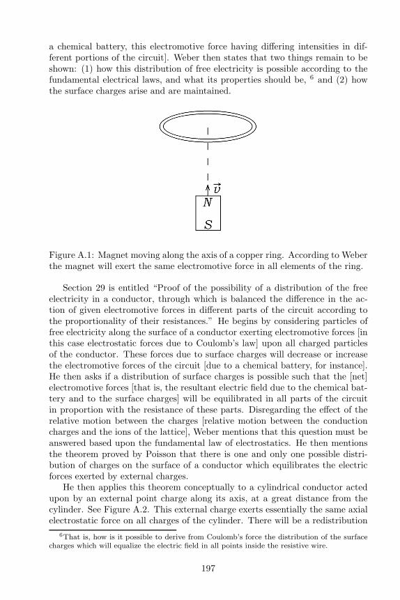
a chemical battery, this electromotive force having differing intensities in dif-ferent portions of the circuit]. Weber then states that two things remain to beshown: (1) how this distribution of free electricity is possible according to thefundamental electrical laws, and what its properties should be, 6 and (2) howthe surface charges arise and are maintained.

Figure A.1: Magnet moving along the axis of a copper ring. According to Weberthe magnet will exert the same electromotive force in all elements of the ring.

Section 29 is entitled “Proof of the possibility of a distribution of the freeelectricity in a conductor, through which is balanced the difference in the ac-tion of given electromotive forces in different parts of the circuit according tothe proportionality of their resistances.” He begins by considering particles offree electricity along the surface of a conductor exerting electromotive forces [inthis case electrostatic forces due to Coulomb’s law] upon all charged particlesof the conductor. These forces due to surface charges will decrease or increasethe electromotive forces of the circuit [due to a chemical battery, for instance].He then asks if a distribution of surface charges is possible such that the [net]electromotive forces [that is, the resultant electric field due to the chemical bat-tery and to the surface charges] will be equilibrated in all parts of the circuitin proportion with the resistance of these parts. Disregarding the effect of therelative motion between the charges [relative motion between the conductioncharges and the ions of the lattice], Weber mentions that this question must beanswered based upon the fundamental law of electrostatics. He then mentionsthe theorem proved by Poisson that there is one and only one possible distri-bution of charges on the surface of a conductor which equilibrates the electricforces exerted by external charges.

He then applies this theorem conceptually to a cylindrical conductor actedupon by an external point charge along its axis, at a great distance from thecylinder. See Figure A.2. This external charge exerts essentially the same axialelectrostatic force on all charges of the cylinder. There will be a redistribution

6That is, how is it possible to derive from Coulomb’s force the distribution of the surfacecharges which will equalize the electric field in all points inside the resistive wire.

197

of charges along the surface of the cylinder, creating an opposite electric fieldand canceling this external force at all internal points of the cylinder. If we nowconsider the presence of this fixed distribution of surface charges, without thepresence of the external point charge [that is, as if the surface charges had beenglued upon the surface of the cylinder and later on the external point chargewere removed], there will be an axial electromotive force acting on all points ofthe cylinder.7

Next he considers a curved cylinder [like a piece of a ring in the form ofan arc of a circle] and a point charge at a great distance from it, along thetangent to one element of the arc. This external point charge exerts a uniformforce along the tangent of the arc, which is equilibrated by the force due to thedistribution of surface charges in the curved cylinder. When this distribution ofsurface charges is kept fixed at their places [by the application of other externalforces to them] and the external point charge is removed, only the longitudinalelectromotive force [acting upon all charges of the cylinder] due to the surfacecharges will remain. He then generalizes this to all elements of the curvedcylinder such that the surface charges on any specific element will be a functionof the surface charges on all other elements of the arc.

Figure A.2: Point charge q along the axis of a finite cylindrical conductor,at a great distance from it. This external charge exerts essentially the sameelectrostatic axial force upon all charges of the cylinder. In equilibrium therewill be an electrical polarization of the cylinder, with the charges along itssurface canceling exactly, at all internal points of the cylinder, the electric fielddue to the external charge.

He then imagines this curved cylinder making a circle, like a ring, with asmall separation between the initial and final cross-sections of the ring. Webershows that these two surfaces should not touch one another; otherwise therewill be an infinite amount of opposite charges on these surfaces (supposing auniform tangential electromotive force acting on all points of the ring). He callsδ the distance between the extremities of the open ring and ±e the charges oftwo elements of these opposite faces. Utilizing Coulomb’s law he shows that theforce on a test charge inside the ring due to the two opposite faces is proportionalto δe. As he wants this electromotive force [or electric field, as we would saytoday] to remain constant as δ → 0, it is necessary that simultaneously e→ ∞,which was what he wanted to prove. The electromotive force along the ring is

7He has proved in this first simple case that there is a distribution of surface charges whichexerts an equal longitudinal force on all points of a cylinder, although he did not explicitlyattempt to calculate the distribution of surface charges in this specific example.

198

then also proportional to δe. In the open region between the two extremities theelectromotive force due to the charges in the end surfaces points in a directionopposite to the direction of the electromotive force acting on a test charge insidethe ring and close to the extremities. He concludes that if we want the sameelectromotive force [net electric field] at all points of the closed ring, then inthe region between the extremities it is necessary for an electromotive forceto act, independent of the distribution of surface charges [that is, a force ofnon-electrostatic origin]. As an example of such a force he mentions the caseof copper and zinc touching one another [we might also mention the case of achemical battery].

He draws three conclusions from these considerations:1. It is not possible to have [steady] current in a closed ring due only to a

distribution of surface charges on the ring. It is necessary to have an electro-motive force of different origin in at least one cross-section of the ring (like thecontact of copper and zinc).8

2. The current in a circuit is proportional to the density of surface chargesalong the circuit.9 The electromotive force is proportional to δe and to thecurrent in the circuit.

3. When we double all dimensions of a circuit but keep the same electro-motive force, then the density of surface charges should remain constant, eventhough the surface area is four times the previous one.10 At the same time itfollows that when we double all dimensions of a circuit, the distance δ shouldalso double, but when the charge e remains constant, the electromotive forceproportional to δe should also double. This double electromotive force requiresthe same motion [velocity] of the charges in a circuit with doubled dimensions,as [the velocity] in a circuit of simple length and cross-section. But this samemotion [velocity] generates four times the current in a circuit with doubled di-mensions (and four times the [area of the] cross-section). That is, a doubledelectromotive force generates, in a circuit of doubled length and four times thecross-section [in comparison with the simple original circuit], a current fourtimes larger, which is in agreement with the laws of the galvanic circuit.

Section 30 is entitled “On the law of the distribution of the free electricity

8This is similar to the theorem that∮

~E · d~ℓ = 0, where ~E is the electrostatic field of

Coulomb’s law, d~ℓ is an element of length and the line integral is over a closed circuit ofarbitrary form. That is, in order to have an electromotive force driving a current around aclosed resistive circuit it is necessary to have a source of non-electrostatic origin. See Section5.1.

9An example of this general conclusion can be seen in Eq. (6.17) for the case of a straightwire. Combining it with Eq. (6.2), σ(z) = σA+σBz/ℓ, yields: I = −(aσB/Rε0) ln(ℓ/a). Thatis, I is directly proportional to σB , as Weber concluded.

10From Eqs. (6.2), (6.14) and with the electric field (Weber’s electromotive force in thiscase) given by E1 = ∆φ/ℓ = RI/ℓ we obtain:

σB =ε0E1

ln(ℓ/a)

ℓ

a. (A.1)

That is, σB is proportional to E1 and to (ℓ/a)/ ln(ℓ/a). If at the same time we double ℓand a, keeping a constant E1, then σB will remain constant. This is an example of Weber’sconclusion.

199

over the surface of a conductor carrying a constant and uniform current.” For alinear conductor he says that we can consider the surface charges as distributedalong its axis.11 He shows this considering a cylindrical conductor of length 2λwith a circular cross-section of radius α≪ λ. See Figure A.3.

Figure A.3: Cylindrical conductor of length 2λ and radius α ≪ λ. In the caseof steady currents, the surface charge density is linear with the longitudinal xcomponent, i.e., proportional to a+ bx.

He considers initially that in the case of a steady current the density ofsurface charges is linear with the longitudinal x component, i.e., proportionalto a+ bx.12 He integrates the longitudinal electromotive force [our electric fieldalong the direction of the axis] due to these surface charges acting on a pointlocated at the origin (the center of the cylinder), obtaining the result (supposingλ≫ α):

∫ λ

x=−λ

2πα(a+ bx)xdx

(α2 + x2)3/2≈ 4παb

(

logλ− logeα

2

)

, (A.2)

where e = 2.7183 is the natural logarithm base.13

He then shows that the same result is obtained when we consider all thesurface charges distributed along the axis of the cylinder, integrating from x =−λ to x = λ, with the exception of the region between x = −eα/2 and x = eα/2.See Figure A.4.

That is, he was able to derive Eq. (A.2) by assuming all surface chargesconcentrated along the axis of the wire and calculating the longitudinal electricfield at the origin integrating from x = −λ to x = −eα/2 and from x = eα/2to x = λ.14

11That is, the actual force exerted by the free charges distributed along the surface of acylindrical conductor carrying a steady current upon a test charge can be replaced by theforce upon this test charge due to an appropriate distribution of charges along the axis of thecylinder.

12Weber’s 2λ and α are equivalent, respectively, to our ℓ and a of Figure 6.1. Weber’s a+bxis equivalent to our σ(z) = σA + σBz/ℓ, Eq. (6.2).

13This result is equivalent to Eq. (6.12), namely, E1 = (aσB/ℓε0) ln(ℓ/ea). All resultsobtained by Weber in this Section can be put in the international system of units by dividingthem by 4πε0. Weber’s log has base e, which means that his log can be written as our ln.In Chapter 6 we first calculated the potential by integration, and then the electric field by~E = −∇φ. Here Weber has integrated the electric field directly. The final result was thesame, as expected.

14 In other words, he considers the line having a linear charge density given by 2πα(a+ bx).He considered the test charge at the origin. This is a very interesting technique which greatlysimplifies the integrations. We have checked his integration and it is correct.

We now generalize his calculation to obtain the longitudinal electric field at an arbitrary

200

Figure A.4: Weber considered now all surface charges distributed along theaxis of the cylinder of length 2λ. According to Weber, the linear integrationthat yields the same electric field at the origin as that given by Figure A.3and Eq. (A.2), now runs from x = −λ to x = λ, except in the region betweenx = −eα/2 and x = eα/2.

point x′, Ex′(x′):

Ex′(x′) =

(

∫ x′−eα/2

x=−λ

+

∫ λ

x=x′+eα/2

)

2πα(a + bx)(x′ − x)dx

[(x′ − x)2]3/2

= −2πα

[

b ln4(λ2 − x′2)

e2α2−

2(a + bx′)x′

λ2 − x′2

]

. (A.3)

At x′ = 0 this yields Weber’s result, namely

Ex′(0) = −4παb ln2λ

eα. (A.4)

We now present an alternative way of obtaining the electric field. This alternative procedurewill be followed by Weber in the calculation of the ring, as we will see shortly.

If he had wished to obtain the electric field from the potential, he would have had tocalculate the potential at a generic point x′ (and not only at the origin x′ = 0). The integralswould need to go from x = −λ to x = x′ − eα/2 and from x = x′ + eα/2 to x = λ. Let uswrite as Φ(x′) the function which would represent the potential at x′ calculated in this way(later on we show that it is different from the real potential φ(x′)). With a charge elementdq = 2πα(a + bx)dx we would obtain:

Φ(x′) =

(

∫ x′−eα/2

x=−λ

+

∫ λ

x=x′+eα/2

)

2πα(a + bx)dx√

(x′ − x)2

= 2πα

[

(a + bx′) ln4(λ2 − x′2)

e2α2− 2bx′

]

. (A.5)

From this expression we obtain

−∂Φ(x′)

∂x′= −2πα

[

b ln4(λ2 − x′2)

e2α2−

2(a + bx′)x′

λ2 − x′2− 2b

]

. (A.6)

And this is different from the electric field given by Eq. (A.3)! For instance, in the limitwhen x′ → 0 Eq. (A.6) yields −4παb ln(2λ/e2α). And there is a difference of 1/e inside thelogarithm as compared with the previous result which Weber obtained by direct integrationof the electric field.

That is, although in general ~E = −∇φ, in this particular case we did not obtain Ex′(x′) =

−∂Φ(x′)/∂x′, as might be expected. The origin of this difference is not easy to locate butwe need to clarify it before proceeding. Everything is due to Weber’s peculiar approximationmethod when we calculate Ex′(x

′) or Φ(x′). In this method the location of the point ofobservation, x′, appears not only in the integrand, but also in the limits of the integrals.The problem arises from the following mathematical result, valid for arbitrary functions andvariables [253, p. 44]:

∂

∂α

∫ x=g(α)

x=f(α)

F (α, x)dx =

∫ x=g(α)

x=f(α)

∂F (α, x)

∂αdx

201

Next he goes to his main calculation. He replaces the straight cylindricalconductor with a toroidal one, like a ring conducting an azimuthal current. Hecalls the greater radius of the ring r and its smaller radius α, supposing α≪ r.He considers the electrostatic potential null at the azimuth angle ψ = π rad anddiscontinuous at ψ = 0 rad. See Figure A.5.

Figure A.5: Conducting ring with greater radius r and smaller radius α, withα ≪ r. The potential is discontinuous at ψ = 0 rad and null at ψ = π rad.Weber wants to calculate the tangential electric field, Eψ, at the angle ψ, Eψ(ψ).The angle ϕ is the variable angle of integration.

That is, the potential F (ψ) [represented by Weber as Fψ] is such that F (0) =−F (2π).15 It is then given by F (ψ) = c(ψ−π), where [F (2π)−F (0)]/2πr = c/ris the value of the tangential electromotive force [our electric field] assumedconstant along the ring. He utilizes his linear approach in order to calculate, in

+

∂g(α)

∂αF [α, g(α)] −

∂f(α)

∂αF [α, f(α)]

. (A.7)

In order to arrive at Eq. (A.3) beginning with Eq. (A.5) we would need to utilize thefollowing expression (obtained from Eq. (A.7)):

Ex′(x′) = −

∂Φ(x′)

∂x′+∂(x′ − eα/2)

∂x′2πα[a + b(x′ − eα/2)]√

[x′ − (x′ − eα/2)]2

−∂(x′ + eα/2)

∂x′2πα[a + b(x′ + eα/2)]√

[x′ − (x′ + eα/2)]2

= −∂Φ(x′)

∂x′− 4παb . (A.8)

And this equation coincides with Eq. (A.3) if we utilize Eq. (A.6). This is the correctapproach if we wish to obtain the electric field E(x′) utilizing Weber’s approximate methodand beginning with an equivalent to a potential function. That is, we need to follow thisapproach if we begin with the function Φ(x′) and wish to obtain E(x′) by differentiation. Wewill return to this point when considering Weber’s next calculation.

15At ψ = 0 rad there should be the point of contact between copper and zinc, or a chemicalbattery, or another non-electrostatic source of electromotive force. Weber’s α, r and F areequivalent to our r0, R0 and φ, respectively. See Fig. 13.1.

202

a general way, the electrostatic potential at the angle ψ along the ring due to allsurface charges, integrating from from ϕ = ψ+ eα/2r to ϕ = 2π+ψ− eα/2r.16

He calls fϕdϕ the amount of free electricity in the arc element rdϕ, wherefϕ is the angular density of free charge (it is not yet specified whether thischarge density is a linear function of the angle ϕ). That is, fϕ is the angulardensity of free electricity along the ring as a function of the azimuth angle ϕ.[From now on we will call it f(ϕ). That is, f(ϕ) has units of charge per angle, orCoulomb per radian in the SI.] He mentions that according to Ohm’s hypothesis,the density of charges along a uniformly resistive conductor should be a linearfunction of the length along the circuit.17 As we have a ring this would imply,according to Weber, that the angular density of charges should be given byf(ϕ) = a(ϕ− π).18 Weber then decides to test if this linear hypothesis is validfor a ring.

Instead of calculating the electric field directly, as he had done in the case ofa linear conductor, he decided to calculate the electrostatic potential.19 To thisend he divides the circumference of radius r into two parts, ABD and DCA.See Figure A.6.

The points A, B, D and C are located at ϕ = 0 rad, ϕ = ψ (where he wants

16That is, instead of performing an integration over the surface of the ring, he performs onlya linear integration replacing the ring by a circumference with an appropriate linear chargedensity. He calculates the potential at the angle ψ, where the test charge will be located. Hisintegration can be thought of as going from ϕ = 0 rad to ϕ = π rad, except for the regionbetween ψ − eα/2r and ψ + eα/2r.

17This can be seen in p. 456 of Ohm’s work [252].18 It should be observed that the a here has no relation with the a of the previous surface

charge density of a cylinder given by a+bx. Weber’s approach is analogous to the one utilizedin Chapter 6. That is, he supposes a distribution of source charges and from them calculatethe potential and electric field. The approach utilized in Chapter 13 was the opposite. InChapter 13 it was given the potential along the surface of the conductor, Laplace’s equationwas solved, yielding the potential everywhere in space. Then the electric field was obtained asminus the gradient of the potential. And finally the surface charges were obtained by applyingGauss’s law at the interface between the conductor and the external medium. For the ringwe obtained a density of surface charges given by Eq. (13.63). Far from the battery this isreduced to Eq. (13.65), namely, σ(ϕ) = σA+ σBϕ/2π. Far from the battery the linear chargedensity which we obtained was given by Eq. (13.74). Weber’s angular density of charges, f(ϕ),is given by R0 times the linear charge density. That is (far from the battery and utilizingη0 ≫ 1, a ≈ R0, a/ sinh η0 = r0 and cosh η0 = R0/r0):

f(ϕ) = R0

(

λA + λBϕ

2π

)

= 2πr0R0

(

σA + σBϕ

2π

)

= 2πR0ε0

[

φA

ln(8R0/r0)+ g(η0)φB

ϕ

2π

]

. (A.9)

Comparing this expression with Weber’s expression, f(ϕ) = a(ϕ−π), we find that Weber’sa is equivalent to our r0R0σB = R0ε0g(η0)φB .

19In principle he would need to integrate

Φ(ψ) ≡[∫ ψ−eα/2r

ϕ=0

+

∫ 2π

ϕ=ψ+eα/2r

]

a(ϕ− π)dϕ

r√

2√

1 − cos(ψ − ϕ). (A.10)

However, if he tried to perform this direct integration he would end up needing to evaluate∫

xdx/ sinx. The solution of this indefinite integral yields an infinite series, namely [203, p.

233]:

203

Figure A.6: Weber’s configuration to integrate the potential.

to know the value of the potential), ϕ = 2ψ and ϕ = ψ + π, respectively. Inorder to calculate the potential at B due to the charges spread along the arcABD, with the exception of the small arc eα/r around B, he considers twocharge elements symmetrically located around B, at angles ±χ from B. Thecharge elements located at ϕ = ψ ± χ, in elementary arcs of length rdχ, aregiven by a(ψ±χ− π)dχ. Each of these charge elements is at the same distance2r sin(χ/2) from B. By adding the contributions of these two charge elementshe obtains the differential potential at B as given by a(ψ − π)dχ/r sin(χ/2).This was a very good idea in order to avoid the integral of xdx/ sinx. Afterintegration he obtains the potential

a(ψ − π)

r

∫ ψ

χ= eα2r

dχ

sin χ2

=2a(ψ − π)

r

(

log tanψ

4− log tan

eα

8r

)

. (A.12)

To obtain the potential at B due to the charges located around the arcDCA he proceeds in a similar way. He considers two charge elements locatedsymmetrically around C, at angles ±χ from C. Relative to A these two chargeelements are located at ϕ = ψ+π±χ. Both are at the same distance 2r sin[(π−ψ)/2)] from B. The potential due to the sum of these two charge elementscalculated at B is then given by aψdχ/r cos(χ/2). After integration he obtains

aψ

r

∫ π−ψ

χ=0

dχ

cos χ2= −2aψ

rlog tan

ψ

4. (A.13)

∫

xdx

sinx= x+

∞∑

k=1

(−1)k+1 2(22k−1 − 1)

(2k + 1)!B2kx

2k+1 . (A.11)

It is difficult to put this infinite series in closed form.Instead of solving this integral directly, Weber utilizes an ingenious approach by taking

advantage of the symmetrical distribution of charges along the circumference, as we will showbelow. In this way he avoids this integral.

204

By adding Eqs. (A.12) and (A.13) he obtains the total potential at ϕ = ψas given by20

−2aψ

rlog tan

eα

8r− 2aπ

r

(

log tanψ

4− log tan

eα

8r

)

. (A.15)

By making the derivative of this expression with respect to the arc rψ,namely, d/rdψ, Weber obtains the following expression for the magnitude ofthe tangential component of the electromotive force [the absolute value of ourelectric field] at the angle ψ due to all surface charges along the ring, except forthe charges in the arc eα/r around ψ:

−2a

r2log tan

eα

8r− aπ

r2 sin(ψ/2). (A.16)

That is, Weber initially calculated the potential at the angle ψ as given byEq. (A.14). He then obtained absolute value of the tangential component of the

20 This final value obtained by Weber can be written as

Φ(ψ) ≡[∫ ψ−eα/2r

ϕ=0

+

∫ 2π

ϕ=ψ+eα/2r

]

a(ϕ − π)dϕ

r√

2√

1 − cos(ψ − ϕ)

= −2aψ

rlog tan

eα

8r−

2aπ

r

(

log tanψ

4− log tan

eα

8r

)

. (A.14)

205

electric field at ψ as given by Eψ(ψ) = dΨψ(ψ)/rdψ, obtaining Eq. (A.16).21

He then mentions that this value is approximately constant only for ψ ≈π rad, i.e., far from the point of discontinuity in the potential [far from thebattery]. When we are close to ψ = 0 rad or to ψ = π rad, the magnitudeof this longitudinal electromotive force is smaller than its magnitude at ψ = πrad. He concludes that Ohm’s hypothesis is only valid for the middle part ofthe circuit (that is, for ψ ≈ π rad).

He mentions that it is then also necessary to consider the charges which arelocated in the cross-sections of the ring where there is a discontinuity in thepotential, charges which had not been considered by Ohm. He calls ±ε theamount of these opposite surface charges (which he considers in his simplifiedmodel as concentrated at points) and δ the small distance separating them. SeeFigure A.7.

After calculating the absolute value of the longitudinal electromotive force[that is, the tangential electric field along the ring] acting at the angle ψ due tothis dipole, Weber obtains the result22

21Weber could have obtained the tangential component of the electric field by direct inte-gration. That is,

Eψ(ψ) =

(∫ ψ−eα/2r

ϕ=0

+

∫ 2π

ϕ=ψ+eα/2r

)

a(ϕ− π) sin(ψ − ϕ)dϕ√

8r2[1 − cos(ψ − ϕ)]3/2

=2a

r2ln tan

eα

8r+

aπ

r2 sin(ψ/2)−eαa

2r31

sin eα4r

. (A.17)

The last term on the right hand side does not appear in Weber’s expression, Eq. (A.16).This is due to the same problem discussed in footnote 14.

In order to arrive at Eq. (A.17) beginning with Eq. (A.14) and taking into account Eq. (A.7),Weber should have utilized:

Eψ(ψ) = −1

r

∂Φ

∂ψ+

∂(ψ − eα/2r)

∂ψ

a(ψ − eα/2r − π)

r2√

2√

1 − cos(ψ − (ψ − eα/2r))

−∂(ψ + eα/2r)

∂ψ

a(ψ + eα/2r − π)

r2√

2√

1 − cos(ψ − (ψ + eα/2r))

= −1

r

∂Φ

∂ψ−

eαa

2r3 sin eα4r

. (A.18)

And this coincides with Eq. (A.17) based on Eq. (A.14).At ψ = π rad and with α≪ r we obtain from Eq. (A.17):

Eψ(ψ = π rad) ≈2a

r2

(

lnα

8r+π

2

)

. (A.19)

Utilizing Weber’s a as our r0R0σB (as we saw in footnote 18) and also his α and r as ourr0 and R0, respectively, the latter equation can be written as (dividing the right hand side by4πε0 in order to obtain the electric field in the international system of units):

Eψ(ψ = π rad) ≈ −r0σB

2πε0R0

(

ln8R0

r0−π

2

)

. (A.20)

22 We have checked this result and it is correct. There should be an overall minus sign infront of this expression if we wish to express the algebraic value of the tangential electric fielddue to this dipole.

206

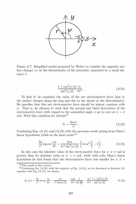
Figure A.7: Simplified model proposed by Weber to consider the opposite sur-face charges ±ε in the discontinuity of the potential, separated by a small dis-tance δ.

1 + cos2(ψ/2)

sin3(ψ/2)

δε

8r3. (A.21)

To find δε he considers the value of the net electromotive force [due tothe surface charges along the ring and due to the dipole at the discontinuity].He specifies that this net electromotive force should be almost constant withψ. That is, he chooses δε such that the second and third derivatives of theelectromotive force with regard to the azimuthal angle ψ go to zero at ψ = πrad. With this condition he obtains23

δε =8aπr

5. (A.22)

Combining Eqs. (A.21) and (A.22) with the previous result arising from Ohm’slinear hypothesis yields as the final result:24

2a

r2log cot

eα

8r+

2aπ

5r2 sin3(ψ/2)

(

3 cos2ψ

2− 2

)

. (A.24)

In this case the absolute value of the electromotive force for ψ 6= π rad isgreater than its absolute value at ψ = π rad, while with only Ohm’s linearhypothesis he had found that the electromotive force was smaller for ψ 6= π

23This result is also correct.24Combining Eq. (A.22) with the negative of Eq. (A.21), as we discussed in footnote 22,

together with Eq. (A.17), we obtain:

Eψ(ψ) =2a

r2ln tan

eα

8r+

aπ

r2 sin(ψ/2)−eαa

2r31

sin eα4r

−aπ

5r21 + cos2(ψ/2)

sin3(ψ/2). (A.23)

207

rad than at ψ = π rad. He then concluded [32] [38, p. 382] (our words insquare brackets): “The correct hypothesis about the distribution of the freeelectricity, from which should result an equal electromotive force [tangential orlongitudinal electric field] in all parts [along the ring] is then contained betweenboth hypotheses above, which means the same as: the [surface] electric charge ofthe circuit increases from the neutral point [ψ = π rad, opposite to the battery]to the contact point [ψ = 0 rad, where there is contact between copper and zinc,or the chemical battery, or another non-electrostatic source of electromotiveforce] not uniformly, but accelerates gradually.”25 He goes on to write: “Theeverywhere equal electromotive force which follows from this [analysis] will besituated presumably between the two limiting values given by the hypothesesabove, namely

2a

r2

(

log coteα

8r− π

2

)

(A.25)

and

2a

r2

(

log coteα

8r− 2π

5

)

. (A.26)

The factor a is related to the slope of the [surface] electric charge in themiddle of the circuit [ψ = π rad], when slope is understood, according to Ohm,as the differential quotient of the charge fϕ [that is, charge per angle f(ϕ)] inrelation to the arc ϕ [in other words, a = df/dϕ].”

In Section 31 Weber presents a mathematical method to estimate the dis-tribution of surface charges in a linear conductor (that is, a filiform conductorwhich can be straight or curved) carrying a steady current, in different cases.His method can also yield an estimation of the magnitude of the correspond-ing electric field inside the conductor produced by this distribution of surfacecharges.

Section 32 is called “Proof of how a necessary distribution of free electricityon the surface of a closed conductor arises when it carries a steady and uniformcurrent.” He considers a closed circuit with only one point acted upon by anelectromotive force [like the contact of copper and zinc]. Only the charges in thispoint will begin to move, but according to Weber, this will cause a distribution offree charges along the whole conductor. And there will be a specific distributionof free charges which will create an electromotive force [electric field] at allother points of the circuit, allowing it to carry a steady current. He goes on tomention that this distribution of surface charges does not produce electrostatic

25That is, he concluded that the surface charge density along the resistive ring carryinga steady current grows linearly with the azimuthal angle ψ only close to ψ = π rad, i.e.,opposite to the battery. When we approach the battery the density of surface charges mustgrow faster than linearly with the azimuthal angle ψ, in order to produce a uniform tangentialelectric field at all points along the ring. That is, the surface charge density cannot increaseas a function of ψ simply as σ = C1 + C2ψ. If it did increase linearly with ψ, the magnitudeof the tangential electric field would not be constant at all points along the ring. This is aremarkable prediction confirmed by our calculations in Chapter 13. See specially Figure 13.7.

208

equilibrium, otherwise the net electric force at any point along the surface of theconductor would be orthogonal to the conductor. He says that this distributionof surface charges will create both a normal component of the electric force atthe surface [of the conductor], and a tangential component. This means, inWeber’s view, that the free charges along the surface of the conductor carryinga steady current cannot be stationary, but must participate in the motion of theinternal current. But he also shows that the motion does not imply a temporalvariation of this distribution of surface charges. That is, this distribution willnot change with time for steady currents, as at any section along the surfacethere will be an equal amount of charges entering and leaving the section. [Thedensity of surface charges will then be a function of the longitudinal coordinateonly, and not a function of time.]

In Section 33 he mentions that during the printing of his work, Kirchhoff’spaper dealing with the same subject was published [24] (this paper has beentranslated into English [27]). We discuss this paper in the next Appendix.Weber quotes the final section of Kirchhoff’s paper. This Section of Weber’swork is important to indicate that Weber and Kirchhoff arrived at essentiallythe same ideas independently of one another, both trying to improve uponOhm’s work and hypotheses. But Weber was the only one who attempted tocalculate explicitly the distribution of surface charges in specific configurations.

Section 34 is called “To determine, through a comparison of electromotiveand galvanometric observations of a galvanic circuit, the relative velocity be-tween two electrical masses in which no attraction nor repulsion arises.” Weberderives here a theoretical relation of the fundamental constant which appears inhis law of force (1846), with the current, resistance and electromotive force ina circuit carrying a steady current. According to Weber’s force law, Eq. (1.1),when two charges approach or separate from from one another with a constantrelative velocity r =

√2c (with the modern nomenclature that c = 3×108 m/s),

they will not affect one another, regardless of the signs of the charges. That is,the Coulombian component of the force will be balanced by the velocity com-ponent, yielding zero net force between them. Only in 1855-56 did Weber andKohlrasch succeed in obtaining experimentally the value of this fundamentalconstant. See Section 1.4 for references.

Section 35 is called “On the ratio of the velocity of the flow to the velocityof the propagation of the current.” Here Weber presents a first theoreticalcomparison of the drifting velocity of charges in a conductor carrying a constantcurrent, with the velocity for the propagation of a variable current along thisconductor. The numerical values of these two velocities were not yet known atthat time, as no experiments had given their orders of magnitude.

Section 36 is called “On the origin of the resistance of conductors.” Hebegins by mentioning that for a complete understanding of the resistance it isnot enough to define it by its effect (as the ratio between electromotive force andcurrent given by Ohm’s law). That is, it is also necessary to define resistanceby its origin. In particular we need to know if it comes through the ponderablepart of the current or from its electric fluid. Weber asks: What is the originof the force that creates resistance to the motion of the charges against the

209

electromotive force accelerating them? He wants to know if this force is purelyelectric, or if it acts upon the ponderable particles of the current (due to forceshaving another origin, like molecular forces). In his reasoning, he considersinitially Fechner’s hypothesis, i.e., he assumes a double current with an equalamount of positive and negative charges moving relative to the wire with equaland opposite velocities. He analyzes whether the encounter of these oppositecharges might give rise to the resistive force, due only to electromagnetic forcesbetween these charges. To this end he considers a simplified model in which onlythe negative charges move relative to the wire, while the positive charges remainfixed in the lattice. He is here departing from Fecher’s hypothesis and comingclose to the modern model of a current in metallic conductors in which onlythe electrons move relative to the lattice. But at that time no one knew aboutthe existence of electrons and they also did not know the order of magnitudeof the drift velocity of the mobile charges. Weber here imagines a negativecharge making a Keplerian elliptical orbit around a positive charge due to acentral force which falls as 1/r2, disregarding the components of his fundamentalforce law (1.1) which depend on the relative velocity and relative accelerationbetween the charges (by considering that these components have a small value incomparison to the greater value of the Coulombian component). When there isan electromotive force [like an external electric field] acting along the wire, it willperturb this orbit into a spiral form. The loops of this spiral will increase untilthe negative charges come into the sphere of action of another positive chargealong the wire. It will orbit this second positive charge until it comes into thesphere of action of the third positive charge along the line composing the wire.This transference of the negative charge to the following positive charges willcontinue as long as the electromotive force acts upon the conductor. In the eventthis electromotive force stops acting, the negative charge will no longer moveforward, but will continue to circle the specific positive charge around whichit was moving when the electromotive force was interrupted. He concludes theSection by mentioning that it would be important to calculate the time intervalneeded by the negative charge to move in its spiral orbit from one positivecharge to the next, but that this calculation should be difficult, as is shown bythe perturbation theory of astronomy.26.

This fifth part of Weber’s paper is extremely important. Here we can see thathe is one of the pioneers who pointed out the surface charges in resistive con-ductors carrying steady currents. The chemical battery or contact between twodifferent metals, like copper and zinc, creates a difference of potential betweentwo points. But what creates the uniform electric field tangential to the circuitat every point inside a resistive wire is the distribution of free charges along

26Weber’s idea that the resistive force might be due to a newtonian central force fallingas 1/r2 does not seem feasible to us for two main reasons. (1) The newtonian forces areconservative and (2) do not depend on the velocities of the interacting bodies. The resistiveforce responsible for Ohm’s law, on the other hand, is non-conservative and proportional tothe drifting velocities of the mobile charges, acting against the motion of these charges. Theorigin of this force must be sought somewhere else. The origin of these resistive forces is avery difficult topic in physics, and even today there is no clear answer to this question.

210

the surface of this wire. He correctly pointed out that these surface chargesmust be in motion together with the current, as the tangential electric field willact not only inside it, but also along the surface of the conductor. Moreover,he was probably the first to try to calculate this distribution of surface chargesexplicitly in a specific example. In particular he considered a ring of finite cross-section, much smaller than the length of the ring, with a small gap at one pointwhere a non-electrostatic electromotive force acts. With an ingenious calcula-tion he showed that the distribution of surface charges increases linearly withthe azimuthal angle only in the region opposite to the battery. He showed thatas we approach the gap the surface charge density must increase faster thanlinearly with the azimuthal angle, a remarkable result confirmed 150 years laterwhen this problem was completely solved analytically, as described in Chapter13 of this book. Weber goes even further, trying to understand the origin of theresistive force in terms of microscopic forces of electromagnetic origin betweenthe interacting charges composing the current. This is a remarkable piece ofwork which deserves to be more widely known.

Weber produced another very important study in 1864 which continues thestudy of surface charges: “Electrodynamic measurements relating specially toelectric oscillations” [254]. This is the fifth work in the series of “Electrodynamicmeasurements.” To the best of our knowledge, it has also never been translatedinto English. The main theoretical derivations of this paper were obtained in1857 or prior to that, but were not published at this time. A similar treatmentwas first published by Kirchhoff in 1857. As we discuss Kirchhoff’s papersin the next Appendix, we will not enter into details here of Weber’s similarfindings which were delayed in publication. Kirchhoff’s paper was published inPoggendorff’s Annalen, now known as Annalen der Physik. Poggendorff wrote anote after Kirchhoff’s paper relating that after seeing it he had occasion to meetWeber in Berlin. Weber showed him the paper he intended to publish, withessentially the same results as Kirchhoff’s. But Weber had not yet sent it toprint, as he was waiting for results of experiments on this topic to be performedtogether with R. Kohlrasch [255]. This paper by Weber was published in 1864.It deals with the propagation of electromagnetic signals along wires, taking intoconsideration variable currents and the effects of all surface charges upon thecurrent. As we will see, Weber and Kirchhoff arrived at the telegraphy equation.

211

212

Appendix B

Gustav Kirchhoff and

Surface Charges

Here we discuss three papers by Kirchhoff, one from 1849 and two from 1857[24, 25, 26]. All of these papers have been translated into English [27, 28, 29].For this reason we present only brief summaries of them.

In the first paper he pointed out a mistake in Ohm’s hypothesis accordingto which a uniform volume density of electricity could remain at rest inside aconductor. Ohm assumed also that the electroscopic or electromotive forces act-ing along a resistive conductor carrying a steady current would be proportionalto the variation of this volume density of charges as regards the longitudinalcoordinate (in the case of a linear conductor). According to Kirchhoff, on theother hand, what is constant inside a conductor in electrostatic equilibrium isits electric potential, but not its volume charge density. The electromotive forceinside a resistive conductor carrying a steady current is proportional to the vari-ation of this potential with the longitudinal coordinate. And the potential itselforiginates from free charges spread along the surface of the conductor. Kirchhoffshows that even in the case of steady currents the potential will satisfy Laplace’sequation inside the conductor. He does not try to calculate the distribution ofthese surface charges in any specific example. At the end of this first paper heshows that Weber’s law of force between point charges is also compatible withOhm’s law, and with his reasoning of free charges along the surface of resistiveconductors.

In his first paper of 1857 Kirchhoff derives the telegraphy equation for a sig-nal propagating along a thin conducting wire. We present here his main resultsin vectorial notation and in the International System of Units SI, following apaper of 1999 [256]. Weber’s simultaneous and more thorough work was delayedin publication, and was published only in 1864. Both worked independently ofone another and predicted the existence of periodic modes of oscillation of theelectric current propagating at light velocity in a conducting circuit of negligibleresistance.

213

In his first paper of 1857, Kirchhoff considered a conducting circuit of circularcross-section which might be open or closed. Kirchhoff’s wire could be straightor curved, provided the following assumption was satisfied: “that the form ofthe central line of the wire is such, that the distance between two of its points,between which a finite portion of the wire lies, is never infinitely small. Bythis supposition the case is excluded, that induction spirals are contained in thecircuit.” He wrote Ohm’s law taking into account the free electricity along thesurface of the wire and the induction due to the alteration of the strength ofthe current in all parts of the wire:

~J = −g(

∇φ+∂ ~A

∂t

)

. (B.1)

Here ~J is the current density, g is the conductivity of the wire, φ is the electricpotential and ~A is a function analogous to the modern magnetic vector poten-tial (which Kirchhoff will calculate from Weber’s force). He calculates φ byintegrating the effect of all free surface charges:

φ(x, y, z, t) =1

4πε0

∫ ∫

σ(x′, y′, z′, t)da′

|~r − ~r ′| . (B.2)

Here ~r = xx + yy + zz is the point where the potential is being calculated,t is the time, and σ is the free surface charge. Kirchhoff then performed aremarkable calculation, integrating this equation over the whole surface of thewire of length ℓ and radius α without specifying the behaviour of σ with regardto the variables x′, y′, z′ or t, but only the requirement that α≪ ℓ. Moreover,he supposed that the current density was the same at all points of the peripheryof a cross-section in the wire (that is, he neglected the effects of curvatures inthe wire) and that it was never infinitely large. With only these assumptionshe arrived finally at:

φ(s, t) =ασ(s, t)

ε0lnℓ

α. (B.3)

Here s is a variable distance along the wire from a fixed origin. See Figure B.1.This is equivalent to our Eq. (6.8). While our equation was derived for a straightwire carrying a steady current, Kirchhoff obtained it for a wire which might bestraight or slightly curved. Moreover, in his calculation the potential, currentand surface charge density could also be a function of time. This was a remark-able result, also obtained by Weber and published in 1864 [254].

He obtains the vector potential ~A from Weber’s force, Eq. (1.1). That is,the component of this force which depends upon the acceleration of the chargescan be written as −q∂ ~A/∂t, with a vector potential given by

~A(x, y, z, t) =µ0

4π

∫ ∫ ∫

[

~J(x′, y′, z′, t) · (~r − ~r ′)]

(~r − ~r ′)dx′dy′dz′

|~r − ~r ′|3 . (B.4)

Here the integration is through the volume of the wire.

214

Figure B.1: A long curved conductor of length ℓ and radius α. The variable srepresents a distance along the wire from a fixed origin O.

After integrating this expression he arrived at

~A(s, t) =µ0

2πI(s, t)

(

lnℓ

α

)

s , (B.5)

where I(s, t) is the variable current.Given that I = Jπα2 and that R = ℓ/(πgα2) is the resistance of the wire,

the longitudinal component of Ohm’s law could then be written as

∂σ

∂s+

1

2πα

1

c2∂I

∂t= − ε0R

αℓ ln(ℓ/α)I . (B.6)

In order to relate the two unknowns, σ and I, Kirchhoff utilized the equationfor the conservation of charges, which he wrote as

∂I

∂s= −2πα

∂σ

∂t. (B.7)

To the best of our knowledge this was the first time that this fundamentalequation for the conservation of charges was published in the literature.

When these two relations are equated, they yield the equation of telegraphy,namely:

∂2ξ

∂s2− 1

c2∂2ξ

∂t2=

2πε0R

ℓ ln(ℓ/α)

∂ξ

∂t, (B.8)

where ξ can represent I, σ, φ or the longitudinal component of ~A.If the resistance is negligible, this equation predicts the propagation of sig-

nals along the wire with light velocity. As Kirchhoff put it, the velocity ofpropagation of an electric wave “is independent of the cross-section, of the con-ductivity of the wire, also, finally, of the density of the electricity: its value is41950 German miles in a second, hence very nearly equal to the velocity of lightin vacuo.”

Equations similar to Eq. (B.8) can be found in pages 123 and 125 of thesecond part of Volume 4 of Weber’s Collected Papers (original paper of 1864)[254, 39].

In his second paper of 1857 Kirchhoff generalizes this first work in orderto consider three-dimensional conductors of arbitrary shape. We discussed this

215

briefly in 1994 [29]. The results are essentially the same as before, but nowhe shows that it is possible to have free electricity distributed throughout thesubstance of the conductor, in the case of a current varying in time and in space.

Recently we developed Kirchhoff’s ideas in the international system of unitsand applied them to the propagation of electromagnetic signals in a coaxialcable, a situation which was not considered by Kirchhoff [30, 31, 257, 258].

It should be stressed that the works of Kirchhoff of 1857 were publishedbefore Maxwell wrote down his equations in 1861-64, establishing the electro-magnetic theory of light. When Maxwell introduced the displacement current(1/c2)∂ ~E/∂t he was utilizing Weber’s constant c. He was also aware of Weberand Kohlrasch’s measurement of 1854-56 that c had the same value as light ve-locity in vacuum. He also knew Kirchhoff’s derivation of the telegraphy equationyielding the propagation of electromagnetic signals at light velocity. Kirchhoff’swork of 1857 was quoted only once by Maxwell in the note to paragraph 805, p.450 of his Treatise [158]. It should be remarked that this specific citation doesnot appear in the Index at the end of Maxwell’s Treatise. For this reason it maynot have been noted by some authors. In note 26 of Schaffer’s paper we find thefollowing important remark regarding Maxwell’s knowledge of Kirchhoff’s firstpaper of 1857: “In the early 1870s Maxwell made detailed notes on Kirchhoff’spaper on electricity in wires: see Cambridge University Library MSS ADD 7655Vn/1, p. 44 ff” [259].

As mentioned above, Kirchhoff’s paper of 1857 was published earlier thanWeber’s paper of 1864, although both of them arrived at essentially the sameresults independently of one another and at the same time, as pointed out byPoggendorff, the editor of the Annalen der Physik (at that time called Poggen-dorff’s Annalen) in 1857 [255].

216

Bibliography

[1] A. K. T. Assis, W. A. Rodrigues Jr., and A. J. Mania. The electric fieldoutside a stationary resistive wire carrying a constant current. Founda-tions of Physics, 29:729–753, 1999.

[2] R. Clausius. Ableitung eines neuen elektrodynamischen Grundgesetzes.Journal fur reine und angewandte Mathematik, 82:85–130, 1877.

[3] A. O’Rahilly. Electromagnetic Theory — A Critical Examination of Fun-damentals. Dover, New York, 1965.

[4] U. Bartocci and M. M. Capria. Some remarks on classical electromag-netism and the principle of relativity. American Journal of Physics,59:1030–1032, 1991.

[5] U. Bartocci and M. M. Capria. Symmetries and asymmetries in classi-cal and relativistic electrodynamics. Foundations of Physics, 21:787–801,1991.

[6] F. Cardone and R. Mignani. Observation of a DC voltage induced by asteady magnetic field: A possible electromagnetic breakdown of Lorentzinvariance? Physics Essays, 13:645–656, 2000.

[7] U. Bartocci, F. Cardone, and R. Mignani. Looking for a possible break-down of local Lorentz invariance for electromagnetic phenomena: theoryand first experimental results. Foundations of Physics Letters, 14:51–64,2001.

[8] J. R. Reitz, F. J. Milford, and R. W. Christy. Foundations of Electromag-netic Theory. Addison-Wesley, Reading, 4th edition, 1993.

[9] B. R. Russell. Surface charges on conductors carrying steady currents.American Journal of Physics, 36:527–529, 1968.

[10] J. D. Jackson. Classical Electrodynamics. John Wiley & Sons, New York,1962.

[11] J. D. Jackson. Classical Electrodynamics. John Wiley & Sons, New York,second edition, 1975.

217

[12] J. D. Jackson. Surface charges on circuit wires and resistors play threeroles. American Journal of Physics, 64:855–870, 1996.

[13] J. D. Jackson. Classical Electrodynamics. John Wiley & Sons, New York,third edition, 1999.

[14] W. F. Edwards. Inertia and an alternative approach to the theory of inter-actions. Proceedings of the Utah Academy of Science, Arts, and Letters,51, Part 2:1–7, 1974.

[15] W. F. Edwards, C. S. Kenyon, and D. K. Lemon. Continuing investiga-tion into possible electric fields arising from steady conduction currents.Physical Review D, 14:922–938, 1976.

[16] D. J. Griffiths. Introduction to Electrodynamics. Prentice Hall, EnglewoodCliffs, second edition, 1989.

[17] C. A. Coombes and H. Laue. Electric fields and charge distributionsassociated with steady currents. American Journal of Physics, 49:450–451, 1981.

[18] P. Lorrain, D. R. Corson, and F. Lorrain. Electromagnetic Fields andWaves. W. H. Freeman and Co., New York, 3rd edition, 1988.

[19] S. Seely. Introduction to Electromagnetic Fields. McGraw-Hill, New York,1958.

[20] B. D. Popovic. Introductory Engineering Electromagnetics. Addison-Wesley, Reading, 1971.

[21] A. K. T. Assis. Deriving Ampere’s law from Weber’s law. HadronicJournal, 13:441–451, 1990.

[22] A. K. T. Assis. Can a steady current generate an electric field? PhysicsEssays, 4:109–114, 1991.

[23] A. K. T. Assis. Weber’s Electrodynamics. Kluwer Academic Publishers,Dordrecht, 1994. ISBN: 0-7923-3137-0.

[24] G. Kirchhoff. Ueber eine Ableitung der Ohm’schen Gesetze, welche sichan die Theorie der Elektrostatik anschliesst. Annalen der Physik, 78:506–513, 1849. Reprinted in G. Kirchhoff’s Gesammelte Abhandlungen (Barth,Leipzig, 1882), pp. 49-55.

[25] G. Kirchhoff. Ueber die Bewegung der Elektricitat in Drahten. Annalender Physik, 100:193–217, 1857. Reprinted in G. Kirchhoff’s GesammelteAbhandlungen (Barth, Leipzig, 1882), pp. 131-154.

[26] G. Kirchhoff. Ueber die Bewegung der Elektricitat in Leitern. Annalender Physik, 102:529–544, 1857. Reprinted in G. Kirchhoff’s GesammelteAbhandlungen (Barth, Leipzig, 1882), pp. 154-168.

218

[27] G. Kirchhoff. On a deduction of Ohm’s law in connexion with the theoryof electrostatics. Philosophical Magazine, 37:463–468, 1850.

[28] G. Kirchhoff. On the motion of electricity in wires. Philosophical Maga-zine, 13:393–412, 1857.

[29] P. Graneau and A. K. T. Assis. Kirchhoff on the motion of electricity inconductors. Apeiron, 19:19–25, 1994.

[30] A. K. T. Assis. On the propagation of electromagnetic signals in wiresand coaxial cables according to Weber’s electrodynamics. Foundations ofPhysics, 30:1107–1121, 2000.

[31] A. K. T. Assis and J. A. Hernandes. Telegraphy equation from Weber’selectrodynamics. IEEE Transactions on Systems and Circuits II, 52:289–292, 2005.

[32] W. Weber. Elektrodynamische Maassbestimmungen insbesondere Wider-standsmessungen. Abhandlungen der Konigl. Sachs. Gesellschaft der Wis-senschaften, mathematisch-physische Klasse, 1:199–381, 1852. Reprintedin Wilhelm Weber’s Werke, Vol. 3, H. Weber (ed.), (Springer, Berlin,1893), pp. 301-471.

[33] R. P. Feynman, R. B. Leighton, and M. Sands. The Feynman Lectures onPhysics. Addison-Wesley, Reading, 1964. Volume 2: Mainly Electromag-netism and Matter.

[34] E. M. Purcell. Electricity and Magnetism, volume 2 of Berkeley PhysicsCourse. McGraw-Hill, New York, 1965.

[35] O. D. Jefimenko. Is magnetic field due to an electric current a relativisticeffect? European Journal of Physics, 17:180–182, 1996.

[36] W. Weber. Wilhelm Weber’s Werke, W. Voigt, (Ed.), volume 1, Akustik,Mechanik, Optik und Warmelehre. Springer, Berlin, 1892.

[37] W. Weber. Wilhelm Weber’s Werke, E. Riecke (Ed.), volume 2, Mag-netismus. Springer, Berlin, 1892.

[38] W. Weber. Wilhelm Weber’s Werke, H. Weber (Ed.), volume 3, Galvanis-mus und Elektrodynamik, first part. Springer, Berlin, 1893.

[39] W. Weber. Wilhelm Weber’s Werke, H. Weber, (Ed.), volume 4, Gal-vanismus und Elektrodynamik, second part. Springer, Berlin, 1894.

[40] W. Weber and E. H. Weber. Wilhelm Weber’s Werke, E. Riecke (Ed.),volume 5, Wellenlehre auf Experimente gegrundet oder uber die Wellentropfbarer Flussigkeiten mit Anwendung auf die Schall- und Lichtwellen.Springer, Berlin, 1893.

219

[41] W. Weber. Wilhelm Weber’s Werke, F. Merkel and O. Fischer (Eds.),volume 6, Mechanik der Menschlichen Gehwerkzeuge. Springer, Berlin,1894.

[42] W. Weber. On the theory of diamagnetism - Letter from Professor Weberto Prof. Tyndall. Philosophical Magazine, 10:407–410, 1855.

[43] W. Weber. On the measurement of electric resistance according to anabsolute standard. Philosophical Magazine, 22:226–240 and 261–269, 1861.

[44] W. Weber. Electrodynamic measurements — Sixth memoir, relating spe-cially to the principle of the conservation of energy. Philosophical Maga-zine, 43:1–20 and 119–149, 1872.

[45] C. F. Gauss and W. Weber. Results of the observations made by theMagnetic Association in the year 1836. In R. Taylor, editor, ScientificMemoirs, Vol. 2, pages 20–97, New York, 1966. Johnson Reprint Corpo-ration.

[46] W. Weber. On the measurement of electro-dynamic forces. In R. Tay-lor, editor, Scientific Memoirs, Vol. 5, pages 489–529, New York, 1966.Johnson Reprint Corporation.

[47] W. Weber. On the excitation and action of diamagnetism according tothe laws of induced currents. In R. Taylor, editor, Scientific Memoirs,Vol. 5, pages 477–488, New York, 1966. Johnson Reprint Corporation.

[48] W. Weber. On the connexion of diamagnetism with magnetism and elec-tricity. In J. Tyndall and W. Francis, editors, Scientific Memoirs, Vol. 7,pages 163–199, New York, 1966. Johnson Reprint Corporation.

[49] W. Weber. Observations on the arrangment and use of the bifilar magne-tometer. In R. Taylor, editor, Scientific Memoirs, Vol. 2, pages 268–280,New York, 1966. Johnson Reprint Corporation.

[50] W. Weber. On a transportable magnetometer. In R. Taylor, editor, Sci-entific Memoirs, Vol. 2, pages 565–586, New York, 1966. Johnson ReprintCorporation.

[51] W. Weber. An extract from remarks on the term-observations for 1839, ofthe German Magnetic Association. In R. Taylor, editor, Scientific Mem-oirs, Vol. 2, pages 587–588, New York, 1966. Johnson Reprint Corpora-tion.

[52] W. Weber. Determinations of electrodynamic measure: particularly inrespect to the connection of the fundamental laws of electricity with thelaw of gravitation. English translation by G. Gregory, unpublished, 21stCentury Science and Technology, 1996.

220

[53] C. F. Gauss and W. E. Weber. Text of the Gauss-Weber correspondence.21st Century, 9(3):41–43, 1996. English translation by Susan P. Johnson.

[54] W. Weber. Aphorisms. 21st Century, 10(2):50–53, 1997. English transla-tion by J. Tennenbaum.

[55] W. Weber and R. Kohlrausch. On the amount of electricity which flowsthrough the cross-section of the circuit in galvanic currents. In F. Bevilac-qua and E. A. Giannetto, editors, Volta and the History of Electricity,pages 287–297. Universita degli Studi di Pavia and Editore Ulrico Hoepli,Milano, 2003.

[56] K. H. Wiederkehr. Wilhelm Webers Stellung in der Entwicklung der Elek-trizitatslehre. Dissertation, Hamburg, 1960.

[57] K. H. Wiederkehr. Wilhelm Eduard Weber — Erforscher der Wellenbewe-gung und der Elektrizitat (1804-1891), volume 32 of Grosse Naturforscher,H. Degen (ed.). Wissenschaftliche Verlagsgesellschaft, Stuttgart, 1967.

[58] K. H. Wiederkehr. Carl Friedrich Gauss (1777-1855) und Wilhelm Weber(1804-1891). In K. v. Meyenn, editor, Die Grossen Physiker, Vol. 1, pages357–370 and 522–524. Verlag C. H. Beck, Munchen, 1997.

[59] F. Kirchner. Determination of the velocity of light from electromagne-tic measurements according to W. Weber and R. Kohlrausch. AmericanJournal of Physics, 25:623–629, 1957.

[60] L. Rosenfeld. The velocity of light and the evolution of electrodynamics.Il Nuovo Cimento, Supplement to vol. 4:1630–1669, 1957.

[61] A. E. Woodruff. The contributions of Hermann von Helmholtz to electro-dynamics. Isis, 59:300–311, 1968.

[62] W. Weber and R. Kohlrausch. Uber die Einfuhrung absoluter elektrischerMaße. In S. Balke, H. Gericke, W. Hartner, G. Kerstein, F. Klemm,A. Portmann, H. Schimank, and K. Vogel, editors, Ostwalds Klassikerder exakten Wissenschaften, new series, Vol. 5. Friedrich-Vieweg & Sohn,Braunschweig, 1968. Commented by F. Kohlrausch and K. H. Wiederkehr.

[63] E. T. Whittaker. A History of the Theories of Aether and Electricity,volume 1: The Classical Theories. Humanities Press, New York, 1973.

[64] L. Rosenfeld. Kirchhoff, Gustav Robert. In C. C. Gillispie, editor, Dic-tionary of Scientific Biography, Vol. 7, pages 379–383, New York, 1981.Charles Scribner’s Sons.

[65] A. E. Woodruff. Weber, Wilhelm Eduard. In C. C. Gillispie, editor,Dictionary of Scientific Biography, Vol. 14, pages 203–209, New York,1981. Charles Scribner’s Sons.

221

[66] K. Reich. Carl Friedrich Gauß — 1777/1977. Heinz Moos Verlag,Munchen, 1977.

[67] M. N. Wise. German concepts of force, energy, and the electromagneticether: 1845–1880. In G. N. Cantor and M. J. S. Hodge, editors, Con-ceptions of Ether — Studies in the History of Ether Theories 1740–1900,pages 269–307, Cambridge, 1981. Cambridge University Press.

[68] P. M. Harman. Energy, Force, and Matter – The Conceptual Developmentof Nineteenth-Century Physics. Cambridge University Press, Cambridge,1982.

[69] C. Jungnickel and R. McCormmach. Intellectual Mastery of Nature —Theoretical Physics from Ohm to Einstein, volume 1-2. University ofChicago Press, Chicago, 1986.

[70] W. A. Atherton. Gauss and Weber: An unlikely partnership. Electronicsand Wireless World, 95:521–522, 1989.

[71] T. Archibald. Energy and the mathematization of electrodynamics inGermany, 1845-1875. Archives Internationales d’Histoire des Sciences,39:276–308, 1989.

[72] K. H. Wiederkehr. Wilhelm Weber und die Entwicklung in der Geomag-netik und Elektrodynamik. In G. Berg, W. Eisenberg, W. Hergert, andH. Thieme, editors, I. Weber - Symposium anlaßlich des 100. TodestagesW. Webers in Halle und Wittenberg am 20. und 21. Juni 1991, pages 1–14. Fachbereich Physik der Martin-Luther-Universitat Halle-Wittenbergund Wilhelm-Weber-Gesellschaft e. V., 1993.

[73] K. H. Wiederkehr. W. Weber und die Entwicklung der Elektrodynamik. InG. Berg, W. Eisenberg, W. Hergert, and W. Schreier, editors, II. Weber- Symposium Die Gebruder Weber - Wegbereiter interdisziplinarer For-shcung in Halle und Leipzig am 16. Oktober und 18. November 1993,pages 39–54. Fachbereich Physik der Martin-Luther-Universitat Halle-Wittenberg und Wilhelm-Weber-Gesellschaft e. V., 1993.

[74] K. H. Wiederkehr. Das Experiment von Wilhelm Weber und RudolfKohlrausch 1855 und Maxwells elektromagnetische Lichttheorie. InW. Schroder, editor, The Earth and the Universe (A Festschrift in hon-our of Hans-Jurgen Treder), pages 452–463. Interdivisional Commissionon History of the International Association of Geomagnetism and Aeron-omy, Bremen-Ronnebeck, 1993.

[75] K. H. Wiederkehr. Wilhelm Weber und Maxwells elektromagnetischeLichttheorie. Gesnerus, Part. 3/4, 51:256–267, 1994.

[76] L. Hecht. Wilhelm Weber: giant of 19th century physics. 21st Century,10(2):53–54, 1997.

222

[77] O. Darrigol. Electrodynamics from Ampere to Einstein. Oxford UniversityPress, Oxford, 2000.

[78] J. P. Wesley. Weber electrodynamics, Part I. General theory, steady cur-rent effects. Foundations of Physics Letters, 3:443–469, 1990.

[79] T. E. Phipps Jr. Toward modernization of Weber’s force law. PhysicsEssays, 3:414–420, 1990.

[80] T. E. Phipps Jr. Weber-type laws of action-at-a-distance in modernphysics. Apeiron, 8:8–14, 1990.

[81] J. P. Wesley. Weber electrodynamics, Part II. Unipolar induction, Z-antenna. Foundations of Physics Letters, 3:471–490, 1990.

[82] J. P. Wesley. Weber electrodynamics, Part III. Mechanics, gravitation.Foundations of Physics Letters, 3:581–605, 1990.

[83] J. P. Wesley. Selected Topics in Advanced Fundamental Physics. BenjaminWesley Publisher, Blumberg, 1991.

[84] R. A. Clemente and A. K. T. Assis. Two-body problem for Weber-likeinteractions. International Journal of Theoretical Physics, 30:537–545,1991.

[85] A. K. T. Assis. Curso de Eletrodinamica de Weber. Setor de Publicacoesdo Instituto de Fısica da Universidade Estadual de Campinas - Unicamp,Campinas, 1992. Notas de Fısica IFGW Numero 5. Available online inPDF format at: http://www.ifi.unicamp.br/˜assis/.

[86] T. E. Phipps Jr. Derivation of a modernized Weber force law. PhysicsEssays, 5:425–428, 1992.

[87] A. K. T. Assis and R. A. Clemente. The ultimate speed implied by theoriesof Weber’s type. International Journal of Theoretical Physics, 31:1063–1073, 1992.

[88] S. Ragusa. Gravitation with a modified Weber force. Foundations ofPhysics Letters, 5:585–589, 1992.

[89] J. Guala-Valverde. Gravitational redshift revisited. Galilean Electrody-namics, 3:58, 1992.

[90] A. K. T. Assis and R. A. Clemente. The influence of temperature ongravitation. Il Nuovo Cimento B, 108:713–716, 1993.

[91] G. Galeczki. The ultimate speed and Weber’s potential. Physics Essays,6:448–450, 1993.

[92] A. K. T. Assis. Eletrodinamica de Weber - Teoria, Aplicacoes e Exercıcios.Editora da Universidade Estadual de Campinas - UNICAMP, Campinas,1995. ISBN: 85-268-0358-1.

223

[93] G. Galeczki and P. Marquardt. Uber die longitudinalen AmpereschenKrafte und Webers Elektrodynamik. Fusion, 16:15–17, 1995.

[94] J. Tennenbaum. An introduction to ‘The significance of the 1845 Gauss-Weber correspondence’. 21st Century, 9(3):2–5, 1996.

[95] L. Hecht. The significance of the 1845 Gauss-Weber correspondence. 21stCentury, 9(3):22–34, 1996.

[96] S. D’Agostino. Absolute systems of units and dimensions of physical quan-tities: a link between Weber’s electrodynamics and Maxwell’s electromag-netic theory of light. Physis, 33:5–51, 1996.

[97] L. Hecht. Experimental apparatus and instrumentation. 21st Century,9(3):35–40, 1996.

[98] T. E. Phipps, Jr. Clock rates in a machian universe. Toth-Maatian Review,13:5910–5917, 1996.

[99] E. T. Kinzer and J. Fukai. Weber’s force and Maxwell’s equations. Foun-dations of Physics Letters, 9:457–461, 1996.

[100] F. Bunchaft and S. Carneiro. Weber-like interactions and energy conser-vation. Foundations of Physics Letters, 10:393–401, 1997.

[101] J. Fukai and E. T. Kinzer. Compatibility of Weber’s force with Maxwell’sequations. Galilean Electrodynamics, 8:53–55, 1997.

[102] A. K. T. Assis. Mecanica Relacional. Editora do Centro de Logica, Episte-mologia e Historia da Ciencia da UNICAMP/FAPESP, Campinas, 1998.ISBN: 85-86497-01-0.

[103] Marcelo Bueno and A. K. T. Assis. Calculo de Indutancia e de For-ca em Circuitos Eletricos. Editora da UFSC/Editora da UEM, Flo-rianopolis/Maringa, 1998. ISBN: 85-328-0119-6.

[104] J. Guala-Valverde. Gravitational mutual energy in Weber-type mechanics.Physics Essays, 11:164–165, 1998.

[105] A. K. T. Assis. Uma Nova Fısica. Editora Perspectiva, Sao Paulo, 1999.ISBN: 85-273-0199-7.

[106] V. F. Mikhailov. The action of an electrostatic potential on the electronmass. Annales de la Fondation Louis de Broglie, 24:161–169, 1999.

[107] A. K. T. Assis. Relational Mechanics. Apeiron, Montreal, 1999. ISBN:0-9683689-2-1.

[108] A. G. Gluckman. On W. E. Weber’s “Grundprincip der Elektrodynamik”and related earlier and contemporary studies. Physics Essays, 12:682–698,1999.

224

[109] J. Guala-Valverde. Inercia y Gravitacion. FundacionJulio Palacios, Neuquen, Argentina, 1999. In collabora-tion with J. Tramaglia and R. Rapacioli. Available at (ac-cessed in 2007): http://www.educ.ar/educar/servlet/Downloads/-S BD LIBROSI/INERCIAYGRAVITACION.PDF.

[110] A. K. T. Assis and H. Torres Silva. Comparison between Weber’s elec-trodynamics and classical electrodynamics. Pramana Journal of Physics,55:393–404, 2000.

[111] A. K. T. Assis and J. Guala-Valverde. Mass in relational mechanics.Apeiron, 7:131–132, 2000.

[112] S. D’Agostino. A History of the Ideas of Theoretical Physics. Kluwer,Dordrecht, 2000.

[113] J. Guala-Valverde. A new theorem in relational mechanics. Apeiron,8:132–138, 2001.

[114] M. d. A. Bueno and A. K. T. Assis. Inductance and Force Calculationsin Electrical Circuits. Nova Science Publishers, Huntington, New York,2001. ISBN: 1-56072-917-1.

[115] V. F. Mikhailov. Influence of an electrostatic potential on the inertialelectron mass. Annales de la Fondation Louis de Broglie, 26:33–38, 2001.

[116] J. Guala-Valverde and P. Mazzoni. The unipolar dynamotor: a genuinerelational engine. Apeiron, 8:41–52, 2001.

[117] R. A. Rapacioli. More about the claimed identity between inertial andgravitational mass. Apeiron, 8:1–9, 2001.

[118] J. P. Wesley. Selected Topics in Scientific Physics. Benjamin WesleyPublisher, Blumberg, 2002.

[119] A. K. T. Assis, K. Reich, and K. H. Wiederkehr. Gauss and Weber’screation of the absolute system of units in physics. 21st Century, 15, No.3:40–48, 2002.

[120] A. K. T. Assis and J. Guala-Valverde. On absolute and relative motionsin physics. Journal of New Energy, 6:8–12, 2002.

[121] J. Guala-Valverde, P. Mazzoni, and R. Achilles. The homopolar motor:A true relativistic engine. American Journal of Physics, 70:1052–1055,2002.

[122] A. K. T. Assis and J. Guala-Valverde. Frequency in relational mechanics.Annales de la Fondation Louis de Broglie, 28:83–97, 2003.

225

[123] V. F. Mikhailov. Influence of a field-less electrostatic potential on theinertial electron mass. Annales de la Fondation Louis de Broglie, 28:231–236, 2003.

[124] A. K. T. Assis and K. H. Wiederkehr. Weber quoting Maxwell. Mitteilun-gen der Gauss-Gesellschaft, 40:53–74, 2003.

[125] J. Fukai. A Promenade Along Electrodynamics. Vales Lake Publishing,Pueblo West, 2003.

[126] J. E. Junginger and Z. D. Popovic. An experimental investigation of theinfluence of an electrostatic potential on electron mass as predicted byWeber’s force law. Canadian Journal of Physics, 82:731–735, 2004.

[127] K. H. Wiederkehr. Ein bisher unveroffentlichter Brief von RudolfKohlrausch an Andreas v. Ettingshausen von 1854, das Kohlrausch-Weber-Experiment von 1854/55 und die Lichtgeschwindigkeit in Wil-helm Webers Elektrodynamik. NTM International Journal of History andEthics of Natural Sciences, Technology and Medicine, 12:129–145, 2004.

[128] D. F. Bartlett. Analogies between electricity and gravity. Metrologia,41:S115–S124, 2004.

[129] A. K. T. Assis, K. Reich, and K. H. Wiederkehr. On the electromagneticand electrostatic units of current and the meaning of the absolute systemof units - For the 200th anniversary of Wilhelm Weber’s birth. SudhoffsArchiv, 88:10–31, 2004.

[130] J. Guala-Valverde. Distant matter in physics. Annales de la FondationLouis de Broglie, 29:635–640, 2004.

[131] J. Guala-Valverde, R. Achilles, and R. Blas. Inertial mass: a changingentity? — Weber vs. Einstein, Weber plus Einstein or none? Apeiron,12:351–352, 2005.

[132] J. P. Wesley and P. Marquardt. Light a Photon Flux and Other Topics.Benjamin Wesley Publisher, Blumberg, 2006.

[133] T. E. Phipps Jr. Old Physics for New - a worldview alternative to Ein-stein’s relativity theory. Apeiron, Montreal, 2006.

[134] W. Weber. Vorwort bei der Ubergabe der Abhandlung: ElektrodynamischeMaassbestimmungen, insbesondere Zuruckfuhrung der Stromintensitats-Messungen auf mechanisches Maass. Berichte uber die Verhandlungen derKonigl. Sachs. Gesellschaft der Wissenschaften zu Leipzig, mathematisch-physische Klasse, 17:55–61, 1855. Reprinted in Wilhelm Weber’s Werke,Vol. 3, H. Weber (ed.), (Springer, Berlin, 1893), pp. 591-596.

226

[135] W. Weber and R. Kohlrausch. Uber die Elektricitatsmenge, welche beigalvanischen Stromen durch den Querschnitt der Kette fliesst. Annalender Physik und Chemie, J. C. Poggendoff (ed.), 99:10–25, 1856. Reprintedin Wilhelm Weber’s Werke, Vol. 3, H. Weber (ed.), (Springer, Berlin,1893), pp. 597-608.

[136] R. Kohlrausch and W. Weber. Elektrodynamische Maassbestimmungeninsbesondere Zuruckfuhrung der Stromintensitats-Messungen auf mecha-nisches Maass. Abhandlungen der Konigl. Sachs. Gesellschaft der Wis-senschaften, mathematisch-physische Klasse, 3:221–290, 1857. Reprintedin Wilhelm Weber’s Werke, Vol. 3, H. Weber (ed.), (Springer, Berlin,1893), pp. 609-676.

[137] W. Weber. Elektrodynamische Maassbestimmungen - uber ein allgemei-nes Grundgesetz der elektrischen Wirkung. Abhandlungen bei Begrundungder Konigl. Sachs. Gesellschaft der Wissenschaften am Tage der zweihun-dertjahrigen Geburtstagfeier Leibnizen’s herausgegeben von der Furstl. Ja-blonowskischen Gesellschaft (Leipzig), pages 211–378, 1846. Reprinted inWilhelm Weber’s Werke, Vol. 3, H. Weber (ed.), (Springer, Berlin, 1893)pp. 25-214.

[138] G. T. Fechner. Ueber die verknupfung der Faraday’schen inductions-erscheinungen mit den Ampereschen elektro-dynamischen erscheinungen.Annalen der Physik, 64:337–345, 1845.

[139] H. C. Oersted. Experiments on the effect of a current of electricity on themagnetic needle. Annals of Philosophy, 16:273–277, 1820.

[140] H. C. Oersted. Experiments on the effect of a current of electricity on themagnetic needle. In R. A. R. Tricker, Early Electrodynamics — The FirstLaw of Circulation, pages 113–117, New York, 1965. Pergamon.

[141] A. M. Ampere. Sur les effets des courans electriques. Annales de Chimie etde Physique, 15:59–76, 1820. Available at: http://www.ampere.cnrs.fr/.

[142] A. M. Ampere. The effects of electric currents. In R. A. R. Tricker, EarlyElectrodynamics - The First Law of Circulation, pages 140–154, New York,1965. Pergamon. Translated by O. M. Blunn.

[143] C. Blondel. A.-M. Ampere el la Creation de l’Electrodynamique (1820-1827). Bibliotheque Nationale, Paris, 1982.

[144] L. P. Williams. What were Ampere’s earliest discoveries in electrodynam-ics? Isis, 74:492–508, 1983.

[145] P. Graneau. Ampere-Neumann Electrodynamics of Metals. HadronicPress, Nonantum, 1985.

[146] J. R. Hofmann. Ampere, electrodynamics, and experimental evidence.Osiris, 3 (2nd Series):45–76, 1987.

227

[147] J. R. Hofmann. Ampere’s invention of equilibrium apparatus: a responseto experimental anomaly. The British Journal for the History of Science,20:309–341, 1987.

[148] J. R. Hofmann. Ampere’s electrodynamics and the acceptability of guidingassumptions. In A. Donovan et al., editor, Scrutinizing Science, pages201–217. Kluwer Academic Publishers, Dordrecht, 1988.

[149] L. P. Williams. Andre-Marie Ampere. Scientific American, January:72–79, 1989.

[150] C. Blondel. Vision physique “etherienne”, mathematisation “laplacienne”:l’electrodynamique d’Ampere. Revue d’Histoire des Sciences, 42:123–137,1989.

[151] P. Graneau and N. Graneau. Newton Versus Einstein – How Matter In-teracts with Matter. Carlton Press, New York, 1993.

[152] P. Graneau. Ampere-Neumann Electrodynamics of Metals. HadronicPress, Palm Harbor, 2nd edition, 1994.

[153] J. R. Hofmann. Andre-Marie Ampere, Enlightenment and Electrodynam-ics. Cambridge University Press, Cambridge, 1996.

[154] P. Graneau and N. Graneau. Newtonian Electrodynamics. World Scien-tific, Singapore, 1996.

[155] T. E. Phipps, Jr. and J. Guala Valverde. Simulation of Amperian currentelements by magnetic toroids. 21st Century, 11:55–65, 1998.

[156] J. Luhr. Die Entstehung eines Demonstrationsexperiments: ZurGeschichte der Ampere’schen Stromwaage. In P. Heering, F. Rieß, andC. Sichau, editors, Im Labor der Physikgeschichte — Zur Untersuchunghistorischer Experimentalpraxis, pages 135–156. BIS der Carl von Ossiet-zky, Oldenburg, 2000.

[157] N. Graneau, T. Phipps Jr., and D. Roscoe. An experimental confirmationof longitudinal electrodynamic forces. European Journal of Physics D,15:87–97, 2001.

[158] J. C. Maxwell. A Treatise on Electricity and Magnetism. Dover, NewYork, 1954.

[159] R. Clausius. Ueber die Vergleichung der elektrodynamische Grundgesetzemit der Erfahrung. Annalen der Physik, 10:608–618, 1880.

[160] F. Rohrlich. Classical Charged Particles — Foundations of Their Theory.Addison-Wesley, Reading, 1965.

[161] R. Skinner. Mechanics. Blaisdell, Waltham, 1969.

228

[162] J. M. Pearson and A. Kilambi. Velocity-dependent nuclear forces andWeber’s electrodynamics. American Journal of Physics, 42:971–975, 1974.

[163] V. Bush. The force between moving charges. Journal of MathematicalPhysics, 5:129–157, 1926.

[164] S. Parker. Electrostatics and current flow. American Journal of Physics,38:720–723, 1970.

[165] R. W. Chabay and B. A. Sherwood. Electric and Magnetic Interactions.Wiley, New York, 1995.

[166] R. W. Chabay and B. A. Sherwood. Matter & Interactions, volume 2:Electric and Magnetic Interactions. Wiley, New York, 2002.

[167] W. G. V. Rosser. Magnitudes of surface charge distributions associatedwith electric current flow. American Journal of Physics, 38:265–266, 1970.

[168] W. K. H. Panofsky and M. Phillips. Classical Electricity and Magnetism.Addison-Wesley, Reading, 2nd edition, 1962.

[169] J. H. Poynting. On the connexion between electric current and the electricand magnetic inductions in the surrounding field. Transactions of theRoyal Society of London A, 176:277–306, 1885.

[170] A. Marcus. The electric field associated with a steady current in longcylindrical conductor. American Journal of Physics, 9:225–226, 1941.

[171] R. W. Chabay and B. A. Sherwood. A unified treatment of electrostaticsand circuits. Unpublished manuscript. Available at (accessed in 2007):http://www4.ncsu.edu/˜rwchabay/mi/circuit.pdf.

[172] L. Bergmann and C. Schaefer. Lehrbuch der Experimentalphysik, volume2: Elektrizitatslehre. Walter de Gruyter, Berlin, 1950.

[173] L. Bergmann and C. Schaefer. Lehrbuch der Experimentalphysik, volume2: Elektrizitat und Magnetismus. Walter de Gruyter, Berlin, seventhedition, 1987.

[174] O. Jefimenko. Demonstration of the electric fields of current-carryingconductors. American Journal of Physics, 30:19–21, 1962.

[175] O. D. Jefimenko. Electricity and Magnetism. Appleton-Century-Crofts,New York, 1966.

[176] O. D. Jefimenko. Electricity and Magnetism. Electret Scientific Company,Star City, 2nd edition, 1989.

[177] O. Jefimenko, T. L. Barnett, and W. H. Kelly. Confinement and shapingof electric fields by current-carrying conductors. Proceedings of the WestVirginia Academy of Science, 34:163–167, 1962.

229

[178] R. Sansbury. Detection of a force between a charged metal foil and acurrent-carrying conductor. Review of Scientific Instruments, 56:415–417,1985.

[179] D. F. Bartlett and S. Maglic. Test of an anomalous electromagnetic effect.Review of Scientific Instruments, 61:2637–2639, 1990.

[180] C. K. Whitney. Current elements in relativistic field theory. PhysicsLetters A, 128:232–234, 1988.

[181] H. Hayden. Possible explanation for the Edwards effect. Galilean Electro-dynamics, 1:33–35, 1990.

[182] T. Ivezic. Electric fields from steady currents and unexplained electro-magnetic experiments. Physical Review A, 44:2682–2685, 1991.

[183] R. C. Ritter and G. T. Gillies. Torsion balances, torsion pendulums, andrelated devices. Review of Scientific Instruments, 64:283–309, 1993.

[184] W. R. Moreau et al. Charge density in circuits. American Journal ofPhysics, 53:552–553, 1985.

[185] R. W. Chabay and B. A. Sherwood. Video demonstrating surfacecharge on a high-voltage circuit. Available at (accessed in 2007):http://www4.ncsu.edu/˜rwchabay/mi/.

[186] D. F. Bartlett and B. F. L. Ward. Is an electron’s charge independent ofits velocity? Physical Review D, 16:3453–3458, 1977.

[187] C. S. Kenyon and W. F. Edwards. Test of current-dependent electricfields. Physics Letters A, 156:391–394, 1991.

[188] G. Bonnet. Electric field arising from a steady current passing through asuperconductor. Physics Letters A, 82:465–467, 1981.

[189] J. C. Cure. A modified version of the Millikan oil drop experiment to testthe probable existence of a new electrodynamic field. Physics Letters B,116:158–160, 1982.

[190] J. P. Wesley. Weber electrodynamics extended to include radiation. Spec-ulations in Science and Technology, 10:47–61, 1987.

[191] R. I. Gray. Unified Physics. Dahlgren, Virginia, 1988.

[192] D. F. Bartlett and W. F. Edwards. Invariance of charge to Lorentz trans-formation. Physics Letters A, 151:259–262, 1990.

[193] T. Ivesic. The relativistic electric fields arising from steady conductioncurrents. Physics Letters A, 144:427–431, 1990.

[194] N. Bilic. Comment on Lorentz invariance/noninvariance of the electriccharge. Physics Letters A, 162:87–90, 1992.

230

[195] D. K. Lemon, W. F. Edwards, and C. S. Kenyon. Electric potentials asso-ciated with steady conduction currents in superconducting coils. PhysicsLetters A, 162:105–114, 1992.

[196] A. K. Singal. On the charge invariance and relativistic electric fields froma steady conduction current. Physics Letters A, 162:91–95, 1992.

[197] V. N. Strel’tsov. The electric field of a current-carrying conductor.Hadronic Journal, 15:457–461, 1992.

[198] G. G. Shishkin et al. Investigation of possible electric potential arisingfrom a constant current through a superconductor coil. Journal of PhysicsD, 35:497–502, 2002.

[199] J. A. Hernandes and A. K. T. Assis. Electric potential due to an infiniteconducting cylinder with internal or external point charge. Journal ofElectrostatics, 63:1115–1131, 2005.

[200] J. C. Maxwell. An Elementary Treatise on Electricity. Clarendon Press,Oxford, 1881.

[201] M. A. Melehy. Thermal momentum in thermodynamics, part 2. interfacialelectrification: a new consequence of the first and second laws. PhysicsEssays, 11:430–433, 1998.

[202] G. B. Arfken and H. J. Weber. Mathematical Methods for Physicists.Academic Press, San Diego, fourth edition, 1995.

[203] I. S. Gradshteyn and I. M. Ryzhik. Table of Integrals, Series, and Products.Academic Press, New York, 5th edition, 1994.

[204] R. N. Varney and L. H. Fisher. Electromotive force: Volta’s forgottenconcept. American Journal of Physics, 48:405–408, 1980.

[205] J. A. Hernandes, E. Capelas de Oliveira, and A. K. T. Assis. Potential,electric field and surface charges close to the battery for a resistive cylin-drical shell carrying a steady longitudinal current. Revista de la Facultadde Ingenierıa (Chile), 12:13–20, 2004.

[206] M. A. Matzek and B. R. Russell. On the transverse electric field withina conductor carrying a steady current. American Journal of Physics,36:905–907, 1968.

[207] W. R. Smythe. Static and Dynamic Electricity. McGraw-Hill, New York,3rd edition, 1968.

[208] A. Sommerfeld. Electrodynamics. Academic Press, New York, 1964.

[209] W. G. V. Rosser. What makes an electric current “flow”. AmericanJournal of Physics, 31:884–885, 1963.

231

[210] W. R. Moreau. Charge distributions on DC circuits and Kirchhoff’s laws.European Journal of Physics, 10:286–290, 1989.

[211] B.-S. Eylon and U. Ganiel. Macro-micro relationships: the missing linkbetween electrostatics and electrodynamics in students’ reasoning. Inter-national Journal of Science Education, 12:79–94, 1990.

[212] C. Schaefer. Einfuhrung in die theoretische Physik, volume 3, part 1.Walter de Gruyter, Berlin, 1932.

[213] B. R. Russell. Surface charges and leaky shields. American Journal ofPhysics, 51:269–270, 1983.

[214] R. N. Varney and L. H. Fisher. Electric field associated with stationarycurrents. American Journal of Physics, 52:1097–1099, 1984.

[215] A. K. T. Assis and J. I. Cisneros. The problem of surface charges and fieldsin coaxial cables and its importance for relativistic physics. In F. Selleri,editor, Open Questions in Relativistic Physics, pages 177–185, Montreal,1998. Apeiron.

[216] A. K. T. Assis and J. I. Cisneros. Surface charges and fields in a resistivecoaxial cable carrying a constant current. IEEE Transactions on Circuitsand Systems I, 47:63–66, 2000.

[217] G. F. Leal Ferreira and Mariangela T. de Figueiredo. A eletrostatica nacorrente eletrica em fios. Revista Brasileira de Ensino de Fısica, 25:374–377, 2003.

[218] J. A. Stratton. Electromagnetic Theory. McGraw-Hill, New York, 1941.

[219] A. K. T. Assis and A. J. Mania. Surface charges and electric field in a two-wire resistive transmission line. Revista Brasileira de Ensino de Fısica,21:469–475, 1999.

[220] A. K. T. Assis, J. A. Hernandes, and J. E. Lamesa. Surface chargesin conductor plates carrying constant currents. Foundations of Physics,31:1501–1511, 2001.

[221] R. Welti. Las cargas superficiales y el flujo de energıa en un circuitosimple. Revista Brasileira de Ensino de Fısica, 27:577–582, 2005.

[222] J. A. Hernandes, E. Capelas de Oliveira, and A. K. T. Assis. Resistiveplates carrying a steady current: electric potential and surface chargesclose to the battery. Foundations of Physics Letters, 18:275–289, 2005.

[223] J. A. Hernandes and A. K. T. Assis. The potential, electric field andsurface charges for a resistive long straight strip carrying a steady current.American Journal of Physics, 71:938–942, 2003.

232

[224] P. Moon and D. E. Spencer. Field Theory Handbook. Springer, Berlin,2nd edition, 1988.

[225] D. J. Griffiths and Y. Li. Charge density on a conducting needle. AmericanJournal of Physics, 64:706–714, 1996.

[226] M. A. Heald. Electric fields and charges in elementary circuits. AmericanJournal of Physics, 52:522–526, 1984.

[227] J. A. Hernandes and A. K. T. Assis. The electric field outside and insidea resistive spherical shell carrying a steady azimuthal current. PhysicaScripta, 72:212–217, 2005.

[228] J. A. Hernandes and A. K. T. Assis. Electric potential for a resistivetoroidal conductor carrying a steady azimuthal current. Physical ReviewE, Vol. 68, 046611, 2003.

[229] J. A. Hernandes and A. K. T. Assis. Surface charges and external electricfield in a toroid carrying a steady current. Brazilian Journal of Physics,34:1738–1744, 2004.

[230] C. Neumann. Theorie der Elektricitats- und Warme-Vertheilung in einemRinge. Verlag der Buchhandlung des Waisenhauses, Halle, 1864.

[231] E. Weber. Electromagnetic Theory – Static Fields and Their Mapping.Dover, New York, 1965. Formerly titled: Electromagnetic Fields, Theoryand Applications.

[232] H. Bateman. Higher Transcendental Functions, volume 1. McGraw-Hill,New York, 1953.

[233] E. Ley-Koo and A. Gongora T. Desarrollo armonico del potencial deCoulomb en coordenadas toroidales. Revista Mexicana de Fısica, 40:805–813, 1994.

[234] E. Weber. Electromagnetic Fields: Theory and Applications, volume 1.Wiley, New York, 1950.

[235] W. R. Smythe. Static and Dynamic Electricity. Hemisphere, New York,3rd edition, 1989.

[236] P. M. Morse and H. Feshbach. Methods of Theoretical Physics, volume 2.McGraw-Hill, New York, 1953.

[237] D. E. Gray (editor). American Institute of Physics Handbook. McGraw-Hill, New York, third edition, 1972.

[238] C. Snow. Formulas for computing capacitance and inductance. NationalBureau of Standards Circular, 544:1–69, 1954.

233

[239] P. Moon and D. E. Spencer. Field Theory for Engineers. Van Nostrand,Princeton, 1961.

[240] O. Jefimenko. Electric fields in conductors. Physics Teacher, 15:52–53,1977.

[241] W. M. Saslow. Consider a spherical batery... American Journal of Physics,62:495–501, 1994.

[242] J. M. Aguirregabiria, A. Hernandez, and M. Rivas. An example of surface-charge distribution on conductors carrying steady currents. AmericanJournal of Physics, 60:138–141, 1992.

[243] J. M. Aguirregabiria, A. Hernandez, and M. Rivas. Surface charges andenergy flow in a ring rotating in a magnetic field. American Journal ofPhysics, 64:892–895, 1996.

[244] H. Hartel. The electric voltage: What do students understand? Whatcan be done to help for a better understanding? In W. JungR. Duit and C. v. Rhoneck, editors, Aspects of Understanding Elec-tricity. Proceedings of an International Workshop, pages 353–362,Kiel, 1985. IPN-Arbeitsberichte 59. Available at (accessed in 2007):http://www.astrophysik.uni-kiel.de/˜hhaertel/PUB/voltage IPN.pdf.

[245] H. Hartel. A qualitative approach to electricity. Institute for Research onLearning, Palo Alto, CA, Report No. IRL87-0001. A revised part of thefull paper is available at (accessed in 2007): http://www.astrophysik.uni-kiel.de/˜hhaertel/PUB/voltage IRL.pdf, 1987.

[246] N. W. Preyer. Transient behavior of simple RC circuits. American Journalof Physics, 70:1187–1193, 2002.

[247] H. Torres S. and A. K. T. Assis. The influence of the electric field outsidea resistive solenoid on the Aharonov-Bohm effect. Revista de la Facultadde Ingenieria de la Universidad de Tarapaca (Chile), 9:29–34, 2001.

[248] D. Psillos, P. Koumaras, and A. Tiberghien. Voltage presented as a pri-mary concept in an introductory teaching sequence on DC circuits. Inter-national Journal of Science Education, 10:29–43, 1988.

[249] A. Benseghir and J.-L. Closset. The electrostatics-electrokinetics tran-sition: historical and educational difficulties. International Journal ofScience Education, 18:179–191, 1996.

[250] B. A. Thacker, U. Ganiel, and D. Boys. Macroscopic phenomena andmicroscopic processes: Students understanding of transients in direct cur-rent electric circuits. American Journal of Physics, 67, Suppl. 1:S25–S31,1999.

234

[251] A. P. French. Newtonian Mechanics. W. W. Norton & Company, NewYork, 1971.

[252] G. S. Ohm. The galvanic circuit investigated mathematically. In R. Tay-lor, editor, Scientific Memoirs, Vol. 2, pages 401–506, New York, 1966.Johnson Reprint Corporation. English translation by W. Francis.

[253] R. K. Pathria. Statistical Mechanics. Pergamon Press, Oxford, 1977.

[254] W. Weber. Elektrodynamische Maassbestimmungen insbesondere uberelektrische Schwingungen. Abh. sachs. Ges. Wiss., 6:105–241, 1864.Reprinted in Wilhelm Weber’s Werke, Vol. 4, H. Weber (ed.), (Springer,Berlin, 1894), pp. 105-241.

[255] J. C. Poggendorff. Bermerkung zu dem Aufsatz des Herrn Prof. Kirchhoff.Annalen der Physik, 100:351–352, 1857. Reprinted in W. Weber’s Werke,Vol. 4, p. 242, H. Weber (ed.), (Springer, Berlin, 1894).

[256] A. K. T. Assis. Arguments in favour of action at a distance. In A. E.Chubykalo, V. Pope, and R. Smirnov-Rueda, editors, Instantaneous Ac-tion at a Distance in Modern Physics - “Pro” and “Contra”, pages 45–56,Commack, 1999. Nova Science Publishers.

[257] J. A. Hernandes and A. K. T. Assis. Propagacao de sinais em condutorescom a eletrodinamica de Weber e comparacao com o eletromagnetismoclassico. In SBF, editor, Anais do XXI Encontro Nacional de Fısica dePartıculas e Campos, Sao Lourenco, 23 a 27/10/00, page 1, Sao Paulo,2000. Sociedade Brasileira de Fısica. Published at (accessed in 2007):http://www.sbf1.if.usp.br/eventos/enfpc/xxi/procs/res89/.

[258] J. A. Hernandes and A. K. T. Assis. Propagacao de sinais em condutoressegundo a eletrodinamica de Weber. Ciencia e Natura, 23:7–26, 2001.

[259] S. Schaffer. Accurate measurement is an english science. In M. NortonWise, editor, The Values of Precision, chapter 6, pages 137–172. PrincetonUniversity Press, Princeton, 1995.

235

Index

Aharonov-Bohm effect, 192, 193Ampere’s

force between current elements,15, 16

law, 16, 19Ampere, A. M., 12, 16Anomalous electromagnetic effect, 36,

37Arfken, G. B., 158Assis, A. K. T., 8, 12, 34, 62

Barnett, T. L., 34, 42, 88, 90, 91,129–131, 185, 193

Bartlett, D. F., 36–40, 43, 87Becquerel, 66Bergmann, L., 30, 31, 34, 36, 42,

88–90, 110, 111, 116, 193Bessel

equation, 53function, 48, 56

Beuzenberg, 40, 42Biot-Savart’s law, 19

Capacitance, 81, 179, 182Cavendish, H., 66Chabay, R. W., 25, 31, 41, 42, 66,

81, 149, 191, 192Charge density

angular, 203linear, 56, 57, 59, 79, 126, 178,

182, 200, 203surface, 8, 11, 21, 24, 26, 27,

40–42, 59, 68, 77, 79–82,85, 86, 89, 94, 107, 108,113, 115, 126–128, 141, 142,145, 146, 153, 158–160, 176–179, 199, 200, 203, 208, 209,

211, 214, 215volume, 8–13, 30, 85, 86, 104,

196, 203, 213Christy, R. W., 9Classical electrodynamics, 3, 20, 22,

26, 84Clausius’s

force, 22, 82postulate, 9

Clausius, R., 9, 10, 17–19Closed circuit, 4, 9, 10, 17–20, 31,

41, 68, 76, 82–84, 157, 191,196, 199, 208, 214

Conservation of charge, 215Coombes, C. A., 11, 81Corson, D. R., 11Coulomb’s

force, 15, 30, 66–68, 195, 197,209, 210

law, 14, 198, 199Current element, 9, 12, 15, 16

Davy, H., 66Dirac delta function, 48Dirichlet boundary condition, 47Displacement current, 216Du Mont power supply, 32

Edwards, W. F., 10, 43Electromagnetic signal, 211, 216Electromotive force, 3, 10, 18, 23,

42, 43, 67, 68, 157, 192,193, 196–200, 202, 205–211,213

Elliptic-cylindrical coordinates, 124Emf, 23, 29, 30, 36, 42, 45, 67, 68,

76, 82, 83, 87, 142, 143,

236

193, 196English translation, 12, 14, 15, 17,

24, 195, 209, 211, 213Equipotential lines, 30, 34, 35, 88–

91, 97, 100, 105, 110, 111,115–117, 119, 121, 128–131,139, 140, 147, 158, 159, 170,171, 183–185, 187, 193

Euler gamma, 175Euler-Mascheroni constant, 57

Faraday cage, 38, 39, 43Faraday’s law of induction, 15Fechner’s hypothesis, 15, 16, 210Fechner, G. T., 15, 19Feynman, R. P., 13, 14, 27Field

electric, 3–5, 8–14, 17, 18, 20–32, 34–36, 40–43, 46, 47,51, 54, 55, 59, 65–67, 69,75–77, 79–91, 93–97, 99–101, 103, 104, 106, 107, 110–113, 115, 117–123, 125–130,139–143, 148, 151, 153, 156–160, 163, 168, 173–177, 181,184–188, 192, 193, 196–203,205, 206, 208, 210, 211

electromagnetic, 26electrostatic, 21, 67, 199Lienard-Wiechert, 10magnetic, 4, 8–10, 12–14, 26,

27, 31, 77, 82, 84, 85, 93,100, 104, 126, 191, 192

Flux of energy, 26Force

electromagnetic, 210, 211Lienard-Schwarzschild, 82magnetic, 12, 84, 85, 109, 110,

126, 127, 186Fourier

series, 50, 139, 143–146, 154,159, 167, 169, 176, 186

transform, 50Fourier, J. B. J., 196French, A. P., 194

Galvaniccircuit, 195, 196, 199, 209current, 17, 18, 195

Ganiel, U., 41, 42Gauss’s

force, 22law, 15, 51, 55, 69, 85, 89, 95,

96, 115, 126, 141, 144, 157,174, 203

Gibbs phenomenon, 167Green function, 47–50, 52, 53Greenwich Meridian, 151Griffiths, D. J., 11, 137

Hartel, H., vi, 192Hall

effect, 16, 67, 77, 82, 84, 85,104, 186

electric field, 126voltage, 84

Hamburg University, iiiHeald, M. A., 137, 140, 146, 192Hernandes, J. A., 37Humboldt Foundation, iii

Inertial frame of reference, 4, 20, 45,65

International System of Units SI, 4,203, 213

Jackson, J. D., 9, 10, 14, 46, 50, 56,155, 163, 183, 191, 192

Jefimenko, O., 13, 14, 31, 32, 34,36, 42, 67, 88–91, 110–113,116, 117, 122, 128–131, 137,184, 185, 187, 191–193

Kelly, W. H., 34, 42, 88, 90, 91, 129–131, 185, 193

Kenyon, C. S., 10, 43Keplerian elliptical orbit, 210Kilambi, A., 19Kirchhoff, G., 4, 12, 24, 77, 90, 192,

209, 211, 213–216Kohlrausch, R., 15, 209, 211, 216Kronecker’s delta funcion, 154, 169

237

Laplace’s equation, 39, 69, 80, 94,95, 123, 125, 138, 153, 166,168, 203, 213

Laue, H., 11, 81Legendre

equation, 153, 166function, 153, 155, 156, 166, 167,

175, 182polynomial, 153, 154, 166

Leighton, R. B., 14, 27Lemon, D. K., 10, 43Lienard-Schwarzschild’s force, 82Lienard-Wiechert

field, 10Light velocity, 10, 29, 66, 213, 215,

216Lines of electric field, 30, 31, 34,

35, 87–91, 95, 97, 110–112,115, 117, 120, 122, 128–130,139–141, 148, 158, 159, 184,185, 187, 193

Lorentz’sforce, 22, 82–84transformation, 14

Lorrain, F., 11Lorrain, P., 11

Maglic, S., 36–40, 87Magnetic

flux, 191vector potential, 193, 214

Magnetic circuital law, 84Matzek, M. A., 84Maxwell, J. C., 17–19, 46, 216Melehy, M. A., 46Method of images, 3, 36, 38, 39, 43,

45, 46, 104, 107, 192Milford, F. J., 9Moreau, W. R., 40, 42, 196Motional electric field, 22, 83, 85, 96

Neumann, C., 164Newton’s second law of motion, 186Newtonian

force, 68, 210Mechanics, 194

Non-Coulomb force, 67, 68, 196

Ohm’s law, 8, 9, 24, 26, 66, 79, 89,94, 98, 103, 109, 123, 137,152, 157, 168, 195, 196, 209,210, 213–215

Ohm, G. S., 196, 203, 206–209, 213Ohmic

conductor, 163, 164, 168resistance, 81, 113toroid, 167

Parker, S., 25, 35, 36, 40, 42, 67Pearson, J. M., 19Poggendorff, J. C., 211, 216Poisson’s equation, 15, 47Poisson, S. D., 197Popovic, B. D., 11, 12Potential difference, 3, 9, 10, 23, 29,

30, 43, 45, 65, 67, 68, 76,81–83, 86, 90, 96, 141, 151,186, 196, 210

Poynting’s vector, 26, 27Poynting, J. H., 26Preyer, N. W., 192Principle of superposition, 65Purcell, E. M., 13, 14

Ratio of electromagnetic and elec-trostatic units of charge, 15

Reitz, J. R., 9Relativistic effect, 13, 14Riecke, 18Riemann, B., 10, 22Ritz, W., 10, 16, 22Rohrlich, F., 19Rosser, W. G. V., 26, 84, 191Russell’s theorem, 68, 135Russell, B. R., 9, 68, 84, 94, 101Ryan, 40, 42

Sands, M., 14, 27Sansbury, R., 30, 36, 37, 39, 40, 42,

86, 88, 89Saslow, W. M., 191Schaefer, C., 30, 31, 34, 36, 42, 67,

88–90, 110, 111, 116, 193

238

Second ordercomponents of Weber’s force, 15correction, 66effect, 10, 21, 87electric field, 10, 12, 20–22, 29,

42, 43, 83, 96, 193force, 20–22, 83, 84, 86, 193

Seely, S., 11Sherwood, B. A., 25, 31, 41, 42, 66,

81, 149, 191, 192Skinner, R., 19Smythe, W. R., 84Sommerfeld, A., 87, 110State University of Campinas - UNI-

CAMP, iiiStratton, J. A., 103Superconductor, 43, 193Syme, 40, 42

Telegraphy equation, 4, 12, 192, 211,213, 215, 216

Toroidal coordinates, 164–166, 173,179, 183

Van de Graaff generator, 32, 67Volta, A. G. A. A., 67Voltage, 3, 7, 8, 10, 12, 17, 18, 20–

23, 25, 30, 32, 36, 40–43,45, 63, 68, 76, 86, 87, 89,98, 142, 143, 193

Ward, B. F. L., 43Weber’s

constant, 216electrodynamics, 10, 12, 14, 16–

20, 22, 82, 83force, 14–17, 19, 82, 83, 209,

213, 214law, iii, 14–17, 19, 20, 43

Weber, H. J., 158Weber, W. E., i, 4, 13–17, 19, 24,

68, 75, 77, 79, 90, 163, 176–178, 188, 191, 192, 194–211,213–216

Weizmann Institute, 41Whittaker, E. T., 18, 19

Wiederkehr, K. H., 14Wronskian, 49, 58

Zeroth ordereffect, 21electric field, 20–22, 29, 43, 46,

51, 59, 87, 192, 193force, 10, 21, 22, 29, 36, 42, 51,

52, 55, 57, 59, 61, 63, 86

239

A. K. T. Assis and J. A. Hernandes, The Electric Force of a Current –

Weber and the Surface Charges of Resistive Conductors Carrying

Steady Currents (Apeiron, Montreal, 2007), ISBN: 978-0-9732911-5-5

Errata

- Page 166, the first line of Eq. (13.6) should read:

coscosh

sinh

sinh

coscosh2

3

2

a

- Page 206, the fourth line should read:

Battery]. When we are close to 0 rad or to 2 rad, the

magnitude

Andre Koch Torres Assis and

Julio Akashi Hernandes

The Electric Force of a Current

Th

e Electric Fo

rce of a C

urren

t

Assis/H

ernan

des

Ap

eiron

About the Authors

Andre Koch Torres Assis was born in Brazil (1962) and educated at the State University of Campinas – UNICAMP, BS (1983), PhD (1987). He spent the academic year of 1988 in England with a post-doctoral position at the Culham Laboratory (United Kingdom Atomic Energy Authority). He spent one year in 1991-92 as a Visiting Scholar at the Center for Electromagnetics Research of Northeastern University (Boston, USA). From August 2001 to November 2002 he worked at the Institute for the History of Natural Sciences, Hamburg University (Hamburg, Germany) with a research fellowship awarded by the Alexander von Humboldt Foundation of Germany. He is the author of Weber’s Electrodynamics (1994), Relational Mechanics (1999); and (with M. A. Bueno) Inductance and Force Calculations in Electrical Circuits (2001). He has been Professor of physics at UNICAMP since 1989, working on the foundations of electromagnetism, gravitation, and cosmology. Julio Akashi Hernandes was born in Brazil (1977) and educated at the State University of Campinas – UNICAMP, BS (1998), MS (2001), PhD (2005). He has always been keenly interested in basic physics, especially electromagnetism. He has published many papers on the electric field outside resistive wires carrying steady currents in major international journals of physics. He is Professor of physics at Universidade Bandeirante de São Paulo, Brazil.

The Electric Force of a Current analyzes the electric force between a charge and a circuit carrying a steady current when they are at rest relative to one another. It presents experiments and analytical calcu-lations showing the existence of this force, contrary to the statements of many scientists. The force is proportional to the voltage of the bat-tery connected to the resistive circuit. It also includes calculations of the potential and electric field inside and outside resistive conductors carrying steady currents, and the distribution of charges along the sur-face of the conductors that generate this field. It contains two appen-dices that discuss the pioneering and revolutionary works of Wilhelm Weber and Gustav Kirchhoff, and a substantial bibliography of mod-ern literature on the topic.

0-9732911-5-X

Weber and the surface charges of resistive conductors carrying steady currents

,!7IA9H3-cjbbff!