ISSN 0956-8549-707

Asset Pricing with Heterogeneous Investors and Portfolio Constraints

By

Georgy Chabakauri

THE PAUL WOOLLEY CENTRE WORKING PAPER SERIES NO 30

FINANCIAL MARKETS GROUP

DISCUSSION PAPER NO 707

July 2012

Georgy Chabakauri is a Lecturer (Assistant Professor) in the Department of Finance at the London School of Economics and Political Science. He received his PhD in Mathematics from Moscow State University in 2004 and his PhD in Finance from London Business School in 2009. His research interests include, asset pricing, portfolio choice, risk management. Any opinions expressed here are those of the author and not necessarily those of the FMG. The research findings reported in this paper are the result of the independent research of the author and do not necessarily reflect the views of the LSE.

Asset Pricing with Heterogeneous Investors andPortfolio Constraints∗

Georgy ChabakauriLondon School of Economics

Houghton StreetLondon WC2A 2AE

United KingdomTel: +44 (0)20 7107 5374Fax: +44 (0)20 7849 4647G.Chabakauri@lse.ac.uk

June 2012

∗I am especially grateful to Suleyman Basak and Anna Pavlova for extensive discussions and comments. I amalso grateful to Pietro Veronesi (the editor) and an anonymous referee, and to Gurdip Bakshi, Harjoat Bhamra,Sudipto Bhattacharya, Andrea Buraschi, Mikhail Chernov, Jaksa Cvitanic, Jerome Detemple (discussant), BernardDumas, Wayne Ferson, Vito Gala, Nicolae Garleanu (discussant), Francisco Gomes, Christopher Hennessy, StevenHeston, Julien Hugonnier, Pete Kyle, Mark Loewenstein, Igor Makarov, Antonio Mele, Antonio Mello, AnthonyNeuberger, Anna Obizhaeva, Stavros Panageas, Marcel Rindisbacher, Raman Uppal, Dimitri Vayanos, MungoWilson, Fernando Zapatero and seminar participants at Econometric Society World Congress, European FinanceAssociation Meetings, Society of Economic Dynamics Meeting, Western Finance Association Meeting, BostonUniversity, Cornell University, Imperial College London, Duisenberg School of Finance, London Business School,London School of Economics, Oxford-Man Institute, University of Lausanne, University of Maryland, University ofSouthern California, University of Toronto, University of Warwick, and University of Zurich for helpful comments.I also thank the Paul Woolley Centre at LSE for financial support. All errors are my responsibility. The previousversion of this paper was circulated under the title “Asset Pricing in General Equilibrium with Constraints.”

Asset Pricing with Heterogeneous Investors andPortfolio Constraints

Abstract

We study dynamic general equilibrium in one-tree and two-trees Lucas economies with oneconsumption good and two CRRA investors with heterogeneous risk aversions and portfolioconstraints. We provide a tractable characterization of equilibrium without relying on the as-sumption of logarithmic constrained investors, popular in the literature, under which wealth-consumption ratios of these investors are unaffected by constraints. In one-tree economy wefocus on the impact of limited stock market participation and margin constraints on marketprices of risk, interest rates, stock return volatilities and price-dividend ratios. We demonstrateconditions under which constraints increase or decrease these equilibrium processes, and gener-ate dynamic patterns consistent with empirical findings. In a two-trees economy we demonstratethat investor heterogeneity gives rise to large countercyclical excess stock return correlations, butmargin constraints significantly reduce them by restricting the leverage in the economy, and giverise to rich saddle-type patterns. We also derive a new closed-form consumption CAPM thatcaptures the impact of constraints on stock risk premia.

Journal of Economic Literature Classification Numbers: D52, G12.Keywords: asset pricing, dynamic equilibrium, heterogeneous investors, portfolio constraints,stochastic correlations, stock return volatility, consumption CAPM with constraints.

Portfolio constraints have long been considered among key market frictions that affect invest-ment decisions and asset prices. Consequently, equilibrium models with investors facing restrictedparticipation, short-sale, leverage, and margin constraints have been widely employed by financialeconomists to explain a wide range of phenomena, such as the equity premium puzzle, mispric-ing of redundant assets, role of arbitrageurs, and comovement of asset returns [e.g., Detempleand Murthy (1997); Basak and Cuoco (1998); Basak and Croitoru (2000, 2006); Gallmeyer andHollifield (2008); Pavlova and Rigobon (2008); Garleanu and Pedersen (2011); among others].Despite recent developments in portfolio optimization, tractable characterizations of equilibriumhave only been obtained at the cost of assuming logarithmic constrained investors, which behavemyopically due to the absence of hedging demands.

The myopia of logarithmic investors allows to study the implications of constraints for marketprices of risk and interest rates, but impedes the evaluation of the impact of constraints on stockprices. As a result, the effects of constraints on stock price-dividend ratios, return volatilities, andcorrelations remain relatively unexplored. The reason is that wealth-consumption ratios of suchinvestors remain constant, and hence unaffected by constraints, since income and substitutioneffects perfectly offset each other. Therefore, these ratios play no role in determining the impactof constraints on stock price-dividend ratios, which in equilibrium are given by the weightedaverage of wealth-consumption ratios of all investors in the economy. For example, in one-stockeconomies populated only by logarithmic investors, stock prices are unaffected by constraints[e.g., Detemple and Murthy (1997); Basak and Cuoco (1998); Basak and Croitoru (2000, 2006)].

In this paper we study the impact of portfolio constraints in both one-tree and two-treesdynamic general equilibrium Lucas (1978) economies with one consumption good, populatedby one unconstrained and one constrained investors that have general constant relative riskaversion (CRRA) preferences. Our model provides a comprehensive analysis of the effects ofconstraints on market prices of risk, interest rates, stock price-dividend ratios, return volatilitiesand correlations. In particular, we demonstrate which constraints generate empirically observeddynamics of equilibrium processes, increase or decrease stock return volatilities and price-dividendratios, and generate excess volatility. In a two-trees economy we derive new consumption CAPMwith constraints, and study stock return correlations.

To provide the intuition for all involved economic forces, we start with a simple one-treeeconomy where both investors have identical risk aversions and one of them faces a limited par-ticipation constraint. This constraint restricts the investment in stocks only to a certain fractionof wealth, and is typical for pension funds.1 Switching off the heterogeneity in risk aversions

1Srinivas, Whitehouse and Yermo (2000) show that limits on both domestic and foreign equity holdings ofpension funds are in place in a number of OECD countries such as Germany (30% on EU and 6% on non-EUequities), Switzerland (30% on domestic and 25% on foreign equities) and Japan (30% on domestic and 30% onforeign equities), among others. Similar constraint arises in models with passive investors that hold up to a fixedfraction of wealth in stocks [e.g., Chien, Cole, and Lustig (2011)], e.g., due to a “status quo bias,” documented inSamuelson and Zeckhouser (1988), or due to the lack of investment skills, as argued in Campbell (2006). Specialcase is restricted participation, when some investors do not participate in the stock market, which in year 2002accounted for 50% of U.S. households [e.g., Basak and Cuoco (1998), Guvenen (2006, 2009)].

1

isolates the pure effect of portfolio constraints, not confounded by investor heterogeneity, whichis not feasible in models with logarithmic investors. We derive all equilibrium processes as func-tions of constrained investor’s share in the aggregate consumption and demonstrate that whenthe substitution effect dominates, the model can generate countercyclical market prices of riskand stock return volatilities, procyclical interest rates and price-dividend ratios, excess volatility,and negative correlation between risk premia and price-dividend ratios, consistently with theliterature [e.g., Shiller (1981); Campbell and Shiller (1988); Schwert (1989); Ferson and Harvey(1991); Campbell and Cochrane (1999)]. We show that tighter constraints always increase marketprices of risk and decrease interest rates, consistently with the previous studies [e.g., Basak andCuoco (1998)]. Furthermore, they increase volatilities and decrease price-dividend ratios whenthe substitution effect dominates, and vice versa when the income effect is stronger.

Intuitively, tighter limited participation constraints increase market prices of risk to inducethe unconstrained investors to hold more stocks in equilibrium, and decrease interest rates sinceconstrained investors allocate more wealth to bonds. As a result, the investment opportunities ofthe constrained investor deteriorate because of falling interest rates, and because the benefits ofhigher market prices of risk are limited due to constraints. If the substitution effect dominates, thewealth-consumption ratio of this investor decreases due to low opportunity cost of consumption,pushing down the price-dividend ratio. The effect of constraints is stronger when the constrainedinvestor accounts for larger fraction of the aggregate consumption. This happens in bad times,when the aggregate dividend is low, since the constrained investor is less exposed to negativedividend shocks. Consequently, the price-dividend ratio becomes procyclical. Moreover, sincestock price is the product of the dividend and the price-dividend ratio, the procyclicality of thelatter amplifies the dividend volatility, making stocks more volatile than dividends.

Next, we consider a richer setting where investors have heterogeneous risk aversions, and theless risk averse investor faces a margin constraint, i.e., is able to borrow only up to a certainfraction of wealth, using stocks as collateral. In this setting the constraint binds intermittently,depending on the amount of liquidity available for borrowing, which is provided by the morerisk averse investor. Tighter constraints lead to deleveraging of the economy, which results inhigher market prices of risk and lower interest rates, similarly to settings with limited participa-tion. Furthermore, we demonstrate that tighter constraints decrease stock return volatilities byreducing the heterogeneity in portfolio strategies of the investors, consistently with the empiricalevidence [e.g., Hardouvelis and Theodossiou (2002)]. We also find that stock return volatilitiesbecome less countercyclical, and spike around the point where constraints start to bind.

Then, we extend the analysis to the case of two-trees Lucas economy with heterogeneousinvestors, where the less risk averse investor faces portfolio constraints. We derive equilibriumprocesses as functions of the shares of the constrained investor and the first Lucas tree in theaggregate consumption. First, we show that heterogeneity in risk aversions significantly increasescorrelations relative to models with homogeneous investors [e.g., Cochrane, Longstaff, and Santa-Clara (2008); Martin (2011)]. In particular, the less risk averse investor scales the portfolio

2

weights up or down, depending on the amount of liquidity supplied by the more risk averseinvestor for borrowing, which increases the correlations. Consistently with the role of liquidity,we show that tighter constraints significantly decrease the correlations by reducing the ability ofthe less risk averse investor to lever up.

We also uncover rich saddle-type patterns in conditional stock return correlations under mar-gin and leverage constraints. Specifically, in a calibration where two trees have the same meanand volatility of dividend growth rates, which are uncorrelated, the constraints lead to a largerfall in correlations when both trees have the same weight in the aggregate dividend. Intuitively,in the latter case, the stocks look symmetric, and hence investors invest equal amount of wealthin each stock. At the same time, the leverage constraint prohibits borrowing, and as a resultinduces investors to invest 50% of their wealth in each stock. Consequently, the heterogeneity intrading strategies is perfectly eliminated, which decreases the correlations towards the homoge-nous investor benchmark. In contrast, when one tree accounts for a large share of aggregatedividend, the stocks have different risk and return characteristics, which generates considerableheterogeneity in trading strategies due to differences in risk aversions, and increases correlations.

In the two-trees economy we provide closed-form expressions for price-dividend ratios in theunconstrained benchmark, and when the investors face leverage constraints, and hence cannotborrow. Therefore, some of the effects of constraints, in particular the time-variation in cor-relations, can be studied using closed-form expressions. In contrast with one-tree economieswith leverage constraint where market prices of risk and stock return volatilities are constant[e.g., Kogan, Makarov, and Uppal (2007)], in our two-trees economy all equilibrium processesare time-varying. We also derive a consumption CAPM with margin constraints in terms ofobservable parameters, which extends Breeden’s (1979) consumption CAPM and Black’s (1972)static mean-variance CAPM with leverage constraint. In the case of a leverage constraint, weobtain a closed-form expression for the deviation from Breeden’s C-CAPM, which captures theinteraction between the heterogeneity in preferences and constraints.

The methodological contribution of the paper is the tractable solution method that provides alaboratory for evaluating the interaction between investor heterogeneity and portfolio constraintswithout relying on investor myopia. The tractability comes from combining the duality approachof Cvitanic and Karatzas (1992) with dynamic programming. First, using the duality approachwe derive equilibrium processes in terms of shadow costs of constraints from the market clearingconditions, as in the literature. Then, we depart from the literature, and instead of finding theshadow costs by solving a dual problem, which is tractable only for logarithmic preferences, wederive them from the complementary slackness conditions in Karatzas and Shreve (1998) in termsof price-dividend and wealth-consumption ratios of investors. Using the dynamic programmingwe then derive a system of differential equations for these ratios, which completely characterizethe equilibrium. The equations are then solved via an iterative procedure with fast convergence.

There is a growing literature that studies dynamic equilibria with constraints. In particu-lar, Detemple and Murthy (1997), Basak and Cuoco (1998), Basak and Croitoru (2000, 2006),

3

Kogan, Makarov, and Uppal (2007), Gallmeyer and Hollifield (2008), Prieto (2010), Garleanuand Pedersen (2011), He and Krishnamurthy (2011), and Hugonnier (2012) consider models withheterogeneous investors where the constrained investor is logarithmic. These works provide atractable settings to study the effect of constraints on market prices of risk and interest rates.However, since wealth-consumption ratios of logarithmic constrained investors are constant, theyplay only a limited role in determining stock prices. For example, in economies where all investorsare logarithmic constraints do not affect stock prices [e.g., Detemple and Murthy (1997); Basakand Cuoco (1998); Basak and Croitoru (2000, 2006)]. In contrast to the previous literature,the constrained investors in this paper have general CRRA utility and significantly affect theformation of stock prices. The generality of our framework also allows us to evaluate the pureeffect of constraints when both investors have identical risk aversions, as well as the interactionbetween investor heterogeneity and portfolio constraints.

This paper is also related to the literature that studies the equilibrium in economies withmultiple stocks. In particular, Pavlova and Rigobon (2008), and Schornick (2009) study modelswith constrained logarithmic investors in international finance model with two Lucas trees. Incontrast to their models, our model does not rely on heterogeneous home bias and logarithmicpreferences. Ribeiro and Veronesi (2002), Menzly, Santos, and Veronesi (2004), Santos andVeronesi (2006), Cochrane, Longstaff, and Santa-Clara (2008), Buraschi, Trojani, and Vedolin(2010), Ehling and Heyerdahl-Larsen (2010), Chen and Joslin (2011) and Martin (2011) studythe unconstrained equilibrium with multiple assets. We contribute to this literature by evaluatingthe impact of constraints, and by providing closed-form expressions for price-dividend ratios inthe case of heterogeneity in risk aversions.

Related works also include Gromb and Vayanos (2002, 2009), Brunnermeier and Pedersen(2009), Fostel and Geanakoplos (2008), and Geanakoplos (2009), which study various implica-tions of margin constraints in different settings. Gromb and Vayanos (2010) survey the relatedliterature on limits to arbitrage. Heaton and Lucas (1996), Cuoco and He (2001), Coen-Pirani(2005), Guvenen (2006, 2009), Gomes and Michaelides (2008), Chien, Cole, and Lustig (2011),Buss and Dumas (2012), Dumas and Lyasoff (2012) solve for equilibrium in various discrete-time incomplete market settings. Other related works include Dumas and Maenhout (2002),Wu (2008), Danielson, Shin, and Zigrand (2009), and Rytchkov (2009) which study the implica-tions of certain types of constraints, such as restricted participation, buy-and-hold, and variousrisk management constraints. Our paper also contributes to growing literature that studies theequilibrium in one-stock economies with heterogeneous unconstrained investors, such as Dumas(1989), Chan and Kogan (2002), Longstaff and Wang (2008), Bhamra and Uppal (2009, 2010),Garleanu and Panageas (2010), Cvitanic and Malamud (2011). Relative to this literature, wedemonstrate how the equilibria are affected by constraints, and provide new closed-form solutionsin unconstrained equilibrium with heterogeneous investors.

The remainder of the paper is organized as follows. Section 1 discusses the economic setupand defines the equilibrium in one-stock economy. In Section 2, we provide the characterization of

4

equilibrium processes, discuss their properties, and describe the solution approach. In Section 3we provide the analysis of equilibrium with limited participation and margin constraints, discussthe economic intuition and implications. Section 4 studies two-stock economies with constraints,derives a consumption CAPM, and evaluates the impact of constraints on stock return correla-tions. Section 5 concludes, Appendix A provides the proofs, Appendix B provides further detailsof our numerical method, and Appendix C discusses the sufficient conditions of optimality.

1. Economic Setup

We consider a continuous-time infinite horizon Lucas (1978) economy with one tree and one con-sumption good. The economy is populated by two heterogeneous investors that, in general, differin risk aversions and portfolio constraints. In this Section we discuss the information structureof the economy, the investors’ optimization, introduce notation, and define the equilibrium.

1.1. Information Structure and Securities Market

The uncertainty is represented by a filtered probability space (Ω, Ft,P), on which is defineda Brownian motion w. The stochastic processes are adapted to the filtration Ft, t ∈ [0,∞)generated by w. The economy is populated by two investors with constant relative risk aversion(CRRA) preferences, indexed by i = A,B, with risk aversions γA and γB, such that γA ≥ γB.There is one tree in the economy that produces Dt units of consumption good at time t, and Dt

follows a geometric Brownian motion (GBM)

dDt = Dt[µDdt+ σDdwt], (1)

where µD ≥ 0 and σD ≥ 0 are constants.

The investors continuously trade in two securities: a riskless bond in zero net supply withinstantaneous interest rate rt and a stock in positive net supply, normalized to one unit, whichis a claim to the stream of output Dt, which we call dividends. We look for Markovian equilibriain which bond prices Bt and stock prices S follow dynamics:

dBt = Btrtdt, (2)dSt +Dtdt = St[µtdt+ σtdwt], (3)

where interest rate r, stock mean return µ, and volatility σ are stochastic processes determinedin equilibrium, and bond price at time 0 is normalized to B0 = 1.

1.2. Investors’ Optimization and Portfolio Constraints

Each investor maximizes expected discounted utility of consumption with time discount ρ > 0:

E[∫ ∞

0e−ρt

c1−γiit

1− γi dt], i = A,B, (4)

5

subject to a self-financing budget constraint, and for investor B subject to a portfolio constraint,given below. For γi = 1 the utility function in (4) is replaced by logarithmic utility ln(cit).

The investors maximize their utility by choosing optimal consumption cit, and an investmentpolicy αit, θit, where αit and θit denote the fractions of wealth invested in bonds and stocks,respectively. Investor i’s wealth process Wit satisfies a dynamic self-financing budget constraint:

dWit =[Wit

(rt + θit(µt − rt)

)− cit

]dt+Witθitσtdwt, i = A,B. (5)

The initial wealth is determined by investors’ endowments at time t = 0: A is endowed with 1−sunits of stock and b units of bond, while B with s units of stock and −b units of bond. Theseendowments are assumed to be consistent with portfolio constraints that the investors may face.

Investor A is unconstrained, while investor B faces the following constraint:

θB ∈ ΘB = θ : θBm ≤ 1, (6)

where m ≥ 0 is the margin parameter. For the simplicity of exposition we assume that marginm isconstant, and discuss the case of stochastic margins in Remark 2 below. The special case of m = 0corresponds to the unconstrained case, while 0 < m ≤ 1 to margin requirements for collateralizedborrowing, when the investor can borrow only up to proportion 1 − m of the stock’s value inthe portfolio [e.g., Brunnermeier and Pedersen (2009); Gromb and Vayanos (2009)]. Special casem = 1 corresponds to a leverage constraint, when investor B is unable to borrow. We note, thatimposing margin constraint with m ≤ 1 also on investor A leaves the equilibrium unchanged sincethis constraint does not bind due to the fact that investor A is more risk averse than investor B.

Furthermore, for 1 < m < +∞ the constraint (6) is interpreted as limited participationconstraint, when investor B is restricted to invest only a small fraction of wealth in stocks. Thelimiting case m = +∞ corresponds to the restricted participation, when investor B does notinvest in the stock market, while m < 0 to a short-sale constraint, discussed in Remark 3 below.

1.3. Equilibrium

In this paper we derive and study the equilibrium market price of risk κ = (µ − r)/σ, interestrate r, volatility σ, price-dividend Ψ = S/D and wealth-consumption Φi = Wi/ci ratios, wherei = A,B. Stock mean return is then given by µ = σκ+ r. We derive all equilibrium processes asfunctions of constrained investor B’s consumption share in the aggregate consumption, y = c∗B/D,which endogenously emerges as a state varaible. We conjecture that y follows an Ito’s process

dyt = −yt[µytdt+ σytdwt], (7)

where the drift µy and volatility σy are endogenously determined in equilibrium.

Definition 1. An equilibrium is a set of processes rt, µt, σt and of consumption and investmentpolicies c∗it, α∗it, θ∗iti∈A,B that maximize expected utility (4) for each investor, given processes

6

rt, µt, σt, and consumption and financial markets clear, i.e.,

c∗At + c∗Bt = Dt,

θ∗AtWAt + θ∗BtWBt = St,

α∗AtWAt + α∗BtWBt = 0,(8)

where WAt and WBt denote time-t wealths of investors A and B, respectively.

2. General Equilibrium with Constraints

In this Section we provide a characterization of equilibrium processes. First, in Section 2.1 weobtain optimal consumptions of investors in a partial equilibrium setting by employing the du-ality approach of Cvitanic and Karatzas (1992). Next, in Section 2.2, from the consumptionclearing condition we obtain equilibrium processes for market prices of risk, interest rates, andstock return volatilities in terms of shadow costs of constraints. These shadow costs are thenfound from complementary slackness conditions in terms of wealth-consumption ratios and theirderivatives. Finally, we derive differential equations for wealth-consumption ratios, which com-pletes the characterization of equilibrium. We also provide the economic intuition for the impactof constraints, and in Section 2.3 discuss the computation of equilibrium.

2.1. Optimal Consumptions in Partial Equilibrium

We start by characterizing optimal consumptions of investors in a partial equilibrium setting,where stock and bond prices are taken as given. Solving the optimization with constraints is achallenging task even at a partial equilibrium level. Here, we follow the approach of Cvitanic andKaratzas (1992), and characterize constrained investors’ optimal consumptions by embedding thepartial equilibrium economy into an equivalent complete-market fictitious economy. We providethe economic intuition for the fictitious economy, and in Remark 1 demonstrate how it can beconstructed via dynamic programming with constrained optimization. Then, we also show howthe complementary slackness conditions emerge from Kuhn-Tucker conditions of optimality.

As demonstrated in Cvitanic and Karatzas (1992), the utility maximization subject to budgetconstraint (5) and portfolio constraint (6) can be solved as an unconstrained optimization in aneconomy with bond and stock prices following dynamics with adjustments:

dBt = Bt[rt + f(νt)]dt, (9)dSt +Dtdt = St[(µt + νt + f(νt))dt+ σtdwt], (10)

where adjustment ν can be interpreted as the shadow cost of portfolio constraint, and f(ν) is the

7

support function for the set of portfolio constraints ΘB, defined as:

f(ν) = supθ∈ΘB

(−νθ). (11)

The adjustments ν can be obtained either by solving a dual optimization problem or from com-plementary slackness conditions, and lie in the effective domain of function f(ν), defined asΥ = ν ∈ R : f(ν) <∞ [e.g., Cvitanic and Karatzas (1992); Karatzas and Shreve (1998)].

In the context of portfolio constraint (6) the intuition behind the fictitious economy is asfollows. When portfolio constraint (6) binds, it reduces the share of wealth that investor Ballocates to stocks, relative to the unconstrained case. This reduction in stock holding can bemimicked in an unconstrained economy with higher interest rates and lower risk premia than inthe original economy. In such a fictitious economy the investor allocates less wealth to stocksthan in the real unconstrained economy, consistently with the policy of the constrained investor.This intuition suggests that for constraint (6) adjustment ν is negative, while f(ν) is positive,which can be confirmed by deriving the support function f(ν) and its effective domain Υ:

f(ν) = −ν∗, ν = ν∗m, Υ = ν∗ : ν∗ ≤ 0. (12)

In complete markets, the drift and volatility of the process for the state price density aregiven by −r and −κ, respectively [e.g. Duffie (2001)], where κ denotes the market price of risk(µ − r)/σ. Therefore, the state price densities in the unconstrained complete-market real andfictitious economies, ξ and ξν∗t, evolve as follows:

dξt = −ξt[rtdt+ κtdwt], dξν∗t = −ξν∗t[(rt − ν∗t )dt+ (κt + ν∗tm/σt)dwt]. (13)

Next, we obtain optimal consumptions of investors from the first order conditions that equatetheir marginal utilities and state price densities [e.g., Huang and Pages (1992); Cuoco (1997)]:

c∗At =(ψAe

ρtξt)− 1

γA , c∗Bt =

(ψBe

ρtξν∗t)− 1

γB , (14)

where ψi denote Lagrange multiplies for static budget constraints in the martingale approach.

Remark 1 (Fictitious Economy and Complementary Slackness Condition). The con-struction of the fictitious economy can be conveniently illustrated via dynamic programming. Inparticular, let JBt denote investor B’s time-t value function, which we conjecture to depend onwealth W , some state variable y, and time t. Let `t denote time-t Lagrange multiplier for port-folio constraint (6), and ν∗t be the rescaled Lagrange multiplier, given by ν∗t = `t/(Wt∂JBt/∂Wt).Then, the value function satisfies the following Hamilton-Jacobi-Bellman (HJB) equation:

0 = maxcBt,θBt

e−ρt

c1−γBBt

1− γBdt+ Et[dJBt] + ν∗t (θBtm− 1)Wt

∂JBt∂Wt

dt,

8

which can be further expanded as follows:

0 = maxcBt, θBt

e−ρt

c1−γBBt

1− γB+ ∂JBt

∂t+[Wt

(rt − ν∗t + θBt(µt − rt + ν∗tm)

)− cBt

]∂JBt∂Wt

−ytµyt∂JBt∂yt

+ 12[W 2t θ

2Btσ

2t

∂2JBt∂W 2

t

− 2WtθBtσtytσyt∂2JBt∂Wt∂yt

+ y2t σ

2yt

∂2JBt∂y2

t

],

(15)

subject to transversality condition Et[JBT ]→ 0, as T →∞. We observe, that equation (15) cor-responds to an HJB equation in the unconstrained fictitious economy with bond and stock pricesfollowing processes (9)–(10), and adjustments ν and f(ν) given by expressions (12). Further-more, Kuhn-Tucker optimality conditions imply that ν∗t ≤ 0, and the complementary slacknesscondition ν∗t (θ∗Btm− 1) = 0 is satisfied.

2.2. Characterization of General Equilibrium

In this subsection we characterize the Markovian equilibrium and discuss its properties. Oursolution approach does not rely on a widely used assumption of a logarithmic constrained investor[e.g., Detemple and Murthy (1997); Basak and Cuoco (1998); Basak and Croitoru (2000, 2006);Kogan, Makarov and Uppal (2003); Gallmeyer and Hollifield (2008); Pavlova and Rigobon (2008);Garleanu and Pedersen (2011); among others] which allows for tractability at the cost of investor’smyopia inherent in logarithmic preferences. We also explain the challenges arising in settingswith non-logarithmic investors, and how these challenges are tackled in this paper. We proceedin three steps, outlined below, while further details are discussed in the proof of Proposition 1.

First, we derive the equilibrium market price of risk κ, interest rate r, volatility σy and driftµy as functions of investor B’s consumption share y and adjustment ν∗ by substituting optimalconsumptions (14) into the consumption clearing condition in (8), applying Ito’s Lemma to bothsides, and matching dt and dw terms. Then, we obtain stock return volatility σ in terms ofvolatility σy, stock price-dividend ratio Ψ, and its derivative Ψ′ by applying Ito’s Lemma toboth sides of equality S = ΨD and matching dw terms. The first step also verifies that κ, r,σy and µy are Markovian in y and ν∗, which endogenously emerge as state variables since thefictitious economy in Section 2.1 can be constructed without assuming specific state variables.Furthermore, adjustment ν∗ is not an independent variable since it can be determined as afunction of consumption share y from Kuhn-Tucker optimality condition for portfolio weight θ∗B ,as discussed below. Therefore, our equilibrium turns out to be Markovian in y.

Next, in the second step, we derive differential equations for wealth-consumption ratios ΦAand ΦB, with coefficients dependant on adjustments ν∗. As demonstrated in Liu (2007), thewealth-consumption ratios satisfy linear PDEs in complete financial markets. Consequently,conditional on knowing the adjustment ν∗, ratios ΦA and ΦB satisfy linear differential equations,since the constrained investor’s optimization is solved in the fictitious complete-market economy.Specifically, following Liu (2007) we conjecture the value functions in the form Ji = W 1−γi

i Φγii /(1−

γi), where i = A,B, substitute them into HJB equations and after some algebra obtain equations

9

for ΦA(y) and ΦB(y). In Appendix C we discuss the sufficient conditions for optimality, andfurther justify the conjectured structure of value functions. The price-dividend ratio Ψ is thenfound from market clearing conditions.

In the third step, most challenging, we complete the characterization of equilibrium by findingadjustment ν∗ from the complementary slackness condition ν∗(θ∗Bm− 1) = 0 [e.g., Karatzas andShreve (1998); Remark 1 in Section 2.1], where portfolio policy θ∗B is given by [e.g., Liu (2007)]:

θ∗Bt = µt − rt + ν∗tmγBσ2

t

− ytσytσt

Φ′B(yt)ΦB(yt)

. (16)

When the constraint does not bind, the complementary slackness condition implies that ν∗ = 0.When the constraint binds, ν∗ is found from equation θ∗Bm = 1, taking into account the expres-sions for volatilities σy and σ identified in the first step in terms of adjustment ν∗. Eventually,we obtain adjustment ν∗ in terms of wealth-consumption ratios ΦA and ΦB, and their derivatives.

The tractability of logarithmic preferences, popular in the literature, is due to the fact thatlogarithmic investor’s wealth-consumption ratio is given by ΦB = 1/ρ, and hence the hedgingdemand (second term) in expression (16) vanishes. The absence of the hedging demand facilitatesfinding adjustment ν∗ from the complementary slackness condition. In particular, when bothinvestors A and B are logarithmic, all equilibrium processes can be identified in closed form.However, in such a setting stock prices are unaffected by constraints, and volatility σ equalsdividend volatility σD [e.g., Detemple and Murthy (1997); Basak and Cuoco (1998)]. The modelis less tractable with non-logarithmic unconstrained investor A, even when investor B remainslogarithmic. In such a setting, κ and r can be found in closed form only in a handful of specialcases, such as restricted participation [e.g., Basak and Cuoco (1998)], short-sale constraint [e.g.,Gallmeyer and Hollifield (2008)], and risk constraint [e.g., Prieto (2010)], while price-dividendratios are obtained numerically by solving linear ODEs.

As demonstrated in Proposition 1 below, price-dividend ratio Ψ is a weighted average ofwealth-consumption ratios of investors, and is given by Ψ = (1− y)ΦA + yΦB. Consequently, theassumption of a logarithmic constrained investor may distort the equilibrium by eliminating theeffects of constraints on wealth-consumption ratio of investor B, who is the one most affected byconstraints. In contrast to the literature, this paper provides a tractable unifying framework forstudying interactions between the heterogeneity in preferences and portfolio constraints withoutrelying on investor myopia. Relaxing the assumption of logarithmic preferences brings neweconomic insights via income and substitution effects that play no role for a logarithmic investor,as elaborated in Section 3. Proposition 1 below summarizes the structure of equilibrium.

Proposition 1. The equilibrium market price of risk κ = (µ− r)/σ, interest rate r, volatility σyand mean growth µy of consumption share y, and stock return volatility σ are given by:

κt = ΓtσD − ΓtytγB

ν∗tmσt

, (17)

10

rt = ρ+ ΓtµD − ΓtΠt

2 σ2D + Γtytν∗t

γB+ ν∗tm

σt

(a1(yt)σD + a2(yt)

ν∗tmσt

), (18)

σyt = Γt(1− yt)γAγB

((γB − γA)σD − ν∗tm

σt

), (19)

µyt = µD − σDσyt − 1 + γB2 (σD − σyt)2 − rt − ν∗t − ρ

γB, (20)

σt = σD − ytσytΨ′(yt)

Ψ(yt), (21)

where a1(y) and a2(y) are functions given by equations (A2) in the Appendix, Γ and Π denotethe risk aversion and prudence parameters of a representative investor,2 and are given by

Γ = γAγBγAy + γB(1− y) , Π = Γ2

(1 + γAγ2A

(1− y) + 1 + γBγ2B

y), (22)

ν∗ is the adjustment given by equation (A4) in the Appendix as a function of price-dividendratio Ψ, wealth-consumption ratio of constrained investor ΦB, and their derivatives. The wealth-consumption ratios ΦA(y) and ΦB(y) satisfy ODEs:

y2σ2y

2 Φ′′A − y(µy + 1− γA

γAκσy

)Φ′A +

(1− γA2γA

κ2 + (1− γA)r − ρ)ΦAγA

+ 1 = 0, (23)

y2σ2y

2 Φ′′B − y(µy + 1− γB

γB

(κ+ ν∗m

σ

)σy)Φ′B

+(1− γB

2γB

(κ+ ν∗m

σ

)2+ (1− γB)(r − ν∗)− ρ

)ΦBγB

+ 1 = 0, (24)

and the price-dividend ratio is given by Ψ(y) = (1− y)ΦA(y) + yΦB(y).

Proposition 1 provides equilibrium processes (17)–(21) in terms of adjustment parameter ν∗,given by expression (A4) in the Appendix in terms of wealth-consumption and price-dividendratios, ΦB and Ψ, respectively. Substituting adjustment ν∗ into equations (23)–(24) we obtaina system of quasilinear ODEs which are solved numerically, as discussed in Section 2.3. Here,we provide the intuition for expressions (17)–(21) by noting that even though ν∗ is not availablein closed form, Kuhn-Tucker conditions imply that ν∗ ≤ 0, and hence its sign is known [e.g.,Cvitanic and Karatzas (1992); Karatzas and Shreve (1998); Remark 1 in Section 2.1].

Since the adjustment is such that ν∗ ≤ 0, expression (17) implies that portfolio constraint(6) increases the market price of risk, if volatility σ is positive (which is confirmed by numericalcomputations). Intuitively, constrained investor B cannot invest in stocks as much as in theunconstrained economy. Consequently, the market price of risk increases to compensate the

2Similarly to Basak (2000, 2005) it can be demonstrated that the equilibrium in this economy is equivalent tothe equilibrium in an economy with a representative investor with a utility function given by:

u(c;λ) = maxcA + cB = c

c1−γAA

1− γA+ λ

c1−γBB

1− γB,

where λ = ξν∗/ξ. The expressions for the relative risk aversion Γ and prudence Π of the representative investor,given by (22), are special cases of those in Basak (2000, 2005), derived for general utility functions.

11

unconstrained investor A for holding more stocks to clear the market. Next, we observe thatinterest rate (18) is a quadratic function of ν∗, and hence the effect of constraint on r is ambiguous.Intuitively, on one hand, the interest rates tend to decrease since the constrained investors havehigher demand for bonds, being unable to invest in stocks. On the other hand, due to the increasein the market price of risk, the unconstrained investors invest more in stocks and less in bonds,which tends to increase the interest rate. In our numerical analysis the former effect dominatesbecause the unconstrained investors are risk averse, and hence the interest rate decreases.

We note that when the horizon is finite the equilibrium can be alternatively characterizedin terms of forward and backward stochastic differential equations (FBSDE), following the samesteps as in the partial equilibrium setting of Detemple and Rindisbacher (2005). In particular,from the expressions for optimal consumptions (14) and the fact that wealth can be representedas the present value of the optimal consumption [e.g., Huang and Pages (1992); Cuoco (1997)],we observe that wealth-consumption ratios are given by:

ΦA(yt) = Et[∫ T

te− ργA

(τ−t)(ξτξt

)1− 1γAdτ], ΦB(yt) = Et

[∫ T

te− ργB

(τ−t)(ξν∗τξν∗t

)1− 1γBdτ], (25)

where ξ and ξν∗ follow processes (13). Derivatives Φ′i(y) can be evaluated via Malliavin calculus[e.g., Detemple, Garcia, and Rindisbacher (2003); Detemple and Rindisbacher (2005)]. Sub-stituting Φ′i(y) into portfolio weights θ∗A and θ∗B, and then using Kuhn-Tucker conditions [e.g.,Karatzas and Shreve (1998); Remark 1 in Section 2.1], leads to a BSDE for adjustment ν∗,similar to equation (3.11) in Detemple and Rindisbacher (2005). Budget constraint (5) gives anadditional forward equation. However, the resulting BSDE is difficult to solve numerically since,in contrast to a partial equilibrium, processes κ, r, σ, and σy also depend on ΦA, ΦB via ν∗.

The unconstrained economy is a convenient benchmark against which we compare our mainresults. We here provide an analytic solution in terms of familiar hypergeometric functions com-monly employed in the literature [e.g., Cochrane, Longstaff, and Santa-Clara (2008); Longstaffand Wang (2008); Longstaff (2009); Martin (2011)]. Our closed-form expressions for equilib-rium quantities generalize the results in Longstaff and Wang (2008), derived under a restrictiveassumption that γA = 2γB. Proposition 2 reports our result.

Proposition 2. In the unconstrained economy market price of risk κ, interest rate r, consump-tion share mean growth µy and volatility σy, and stock return volatility σ are given in closed form

12

by expressions (17)–(21) in which ν∗ = 0, and the price-dividend ratio Ψ is given by:

Ψ(y) = 1p

[− 1γA + ϕ−

2F1

((1− γB

γA

)ϕ− − γB, 1, 1− γB −

γBγAϕ−; y

)

+(1− γB

γA

) y

1− γB − γBγAϕ−

2F1

((1− γB

γA

)ϕ− + 1− γB, 1, 2− γB − γB

γAϕ−; y

)

+ γBγA

1ϕ+

2F1

((1− γB

γA

)ϕ+ − γB, 1, 1 + ϕ+; 1− y

)

+(1− γB

γA

) y

ϕ+2F1

((1− γB

γA

)ϕ+ + 1− γB, 1, 1 + ϕ+; 1− y

)],

(26)

where constants p, ϕ+ and ϕ− are given in closed form by expressions (A22) in Appendix A, and2F1(x1, x2, x3; y) denotes a hypergeometric function, given in Appendix A.

Remark 2 (Time-varying Margins). Propositions 1 and Lemma A.1 in the Appendix remainvalid without any changes for time-varying margins that depend on equilibrium processes, e.g.,m = m(yt, σt). Such margins may arise in the case of constraints on portfolio volatility, or whenmargins tighten in periods of high volatility. In this work, for expositional simplicity, we assumethat margins are constant, and focus on exploring the implications of the tightness of constraintson equilibrium. At the end of the proof of Lemma A.1 in Appendix A we elaborate on howadjustment ν∗ can be computed when margin m is a function of volatility.

Remark 3 (Short-sale Constraints). We note that short-sale constraint θB ≥ θ, where θ < 0,is a special case of constraint (6) when m < 0. However, to make the constraint binding, themodel requires the heterogeneity in beliefs about mean dividend growth µD arising, e.g., dueto differences in time-0 priors [e.g., Basak (2000, 2005)]. The model can be easily solved wheninvestors A and B believe that the mean dividend growth is constant, and equals µA,D andµB,D, respectively, and do not update their beliefs. As argued in Abel (2002) and Colacito andCroce (2012), dogmatic beliefs and persistent disagreement can be rationalized when investorsfear model misspecification and solve their optimisation using robust control [e.g., Hansen andSargent (2007)]. Incorporating learning into this model is an interesting but challenging problem,which increases the dimensionality of equations by introducing extra state and time variables.

2.3. Boundary Conditions and Computation of Equilibrium

In this subsection we briefly discuss the computation of equilibrium, while further detailsare presented in Appendix B. First, we discuss the boundary conditions for ODEs (23)–(24).These conditions provide further insights on the dependence of wealth-consumption ratios on thetightness of constraints, and conditions for the constraint to be binding in the economy. Then,we describe the numerical method, based on finite differences approach. Here, we only considerthe case of margin constraints with m < 1, while the case m ≥ 1 is addressed in Appendix B.

13

Following the literature [e.g., Duffy (2006); Garleanu and Pedersen (2011)] we obtain bound-ary conditions by passing to limits in ODEs (23)–(24) as y → 0 and y → 1 [see Appendix B].Intuitively, these conditions coincide with wealth-consumption ratios in the limiting economiesdominated by investor A (as y → 0) and B (as y → 1), respectively. We note, that the marginconstraint does not bind when constrained investor B dominates (i.e, y ≈ 1). The reason is thatbinding constraint θB = 1/m > 1 would violate the market clearing in stocks in such an economy.Consequently, the market price of risk κ and the interest rate r in the limiting economies coincidewith those in respective homogeneous-investor unconstrained economies.

The analysis of investor optimization in the limiting economies gives boundary conditions:

ΦA(0) = γA

ρ− 1− γA2γA

κ2A − (1− γA)rA

, ΦA(1) = γA

ρ− 1− γA2γA

κ2B − (1− γA)rB

,

ΦB(0) = γB

ρ− 1− γB2γB

(κA + ν∗m

σD

)2− (1− γB)(rA − ν∗), ΦB(1) = γB

ρ− 1− γB2γB

κ2B − (1− γB)rB

,(27)

where κi and ri denote the market price of risk and interest rate in the unconstrained homogeneous-agent economy populated by investor i, ν∗ = ν∗(0), and these quantities are given by:

κi = γiσD, ri = ρ+ γiµD − γi(1 + γi)2 σ2

D , i = A,B, (28)

ν∗ =(σDm

)2min(0, γB − γAm). (29)

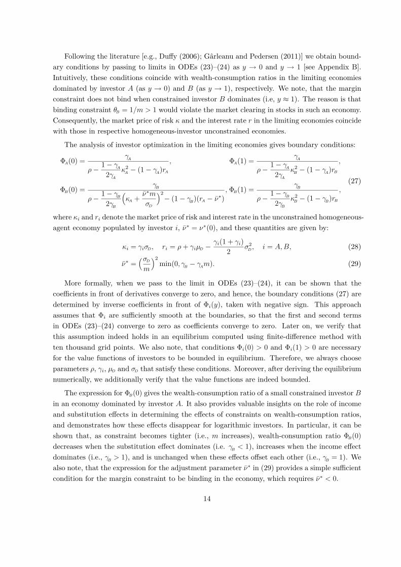
More formally, when we pass to the limit in ODEs (23)–(24), it can be shown that thecoefficients in front of derivatives converge to zero, and hence, the boundary conditions (27) aredetermined by inverse coefficients in front of Φi(y), taken with negative sign. This approachassumes that Φi are sufficiently smooth at the boundaries, so that the first and second termsin ODEs (23)–(24) converge to zero as coefficients converge to zero. Later on, we verify thatthis assumption indeed holds in an equilibrium computed using finite-difference method withten thousand grid points. We also note, that conditions Φi(0) > 0 and Φi(1) > 0 are necessaryfor the value functions of investors to be bounded in equilibrium. Therefore, we always chooseparameters ρ, γi, µD and σD that satisfy these conditions. Moreover, after deriving the equilibriumnumerically, we additionally verify that the value functions are indeed bounded.

The expression for ΦB(0) gives the wealth-consumption ratio of a small constrained investor Bin an economy dominated by investor A. It also provides valuable insights on the role of incomeand substitution effects in determining the effects of constraints on wealth-consumption ratios,and demonstrates how these effects disappear for logarithmic investors. In particular, it can beshown that, as constraint becomes tighter (i.e., m increases), wealth-consumption ratio ΦB(0)decreases when the substitution effect dominates (i.e. γB < 1), increases when the income effectdominates (i.e., γB > 1), and is unchanged when these effects offset each other (i.e., γB = 1). Wealso note, that the expression for the adjustment parameter ν∗ in (29) provides a simple sufficientcondition for the margin constraint to be binding in the economy, which requires ν∗ < 0.

14

Next, we solve for equilibrium using finite difference method. The solution method is com-plicated by the quasilinearity of ODEs (23)–(24), since the adjustment ν∗ is itself a function ofΦi, Ψ, and their derivatives. We circumvent this difficulty by using two approaches suggestedin the literature. The first one is the fixed point iteration method [e.g., Gomes and Michaelides(2008); Guvenen (2009); Chien, Cole and Lustig (2011); among others], in which we use can-didate wealth-consumption ratios Φi,k(y) at step k to compute all the equilibrium processes,including the adjustment ν∗. Then, we note, that ODEs (23)–(24) become linear conditional onknowing the equilibrium processes and the adjustment. Accordingly, we obtain next-step wealthconsumption ratios by solving these linear ODEs numerically. Then, we calculate the impliedequilibrium processes again, and iterate until convergence. This method typically gives very fastconvergence if the conjectured wealth-consumption ratios at step 0 are not very far from theequilibrium ones.

We note that this convergence is reminiscent of well-known tatonnement dynamics [e.g.,Mas-Colell, Whinston, and Green (1995)], which describes the transition of the economy fromdisequilibrium to equilibrium. In particular, similarly to tatonnement dynamics, we start withdisequilibrium processes, observe how they get incorporated into wealth-consumption ratios,which via the market clearing conditions translate into equilibrium processes at the next step.Consequently, the convergence of the numerical algorithm is an intuitive property of equilibria,which are resilient to perturbations in the equilibrium processes.

The second approach is inspired by the method of successive iterations for solving the equa-tions of dynamic programming [e.g., Ljungqvist and Sargent (2004)], when the value functionis set equal to a certain function at a distant horizon T and then the value functions at earlierdates are obtained by solving equations backwards. This approach is just a version of the firstone, and in Appendix B we argue that it adds stability to the solution method. More specifi-cally, we consider a finite-horizon problem with a large horizon parameter T , choose a terminalvalue for Φi(y, T ) and then solve the equations backwards in time using a modification of Euler’sfinite-difference method until the solutions converge to time-independent functions Φi(y).

To solve the differential equations we replace derivatives by their finite-difference analogues,then sitting at time t we compute the coefficients of finite-difference equations using the solutionsobtained from the previous step t+ ∆t. As a result, at step t the coefficients of the equations forwealth-consumption ratios are known, and hence Φi can be found by solving a system of linearfinite-difference equations with a three-diagonal matrix. In most of the cases studied in thispaper we use fixed point iterations while in certain cases we use a combination of two methodsto facilitate the convergence. Appendix B provides further details.

In Appendix C we also discuss some sufficient conditions for the optimality of investors’consumption and portfolio strategies, which are easy to verify once the equilibrium processesare computed numerically. We show that these sufficient conditions are satisfied in economieswith margin constraints, where all equilibrium processes are continuous and uniformly bounded[e.g., Figure 3 in Section 3.2]. However, the case of limited participation is not covered by our

15

verification result since the processes have a singularity at y = 1 [e.g., Figures 1 and 2 in Section3.1], and may require more subtle sufficient conditions, which are not available in the literature.

3. Analysis of Equilibrium

In Sections 3.1 and 3.2 below, we explore the asset pricing implications of limited participationand margin constraints, respectively. The earlier literature primarily focused on the impact ofvarious special cases of portfolio constraint (6) on market prices of risk κ and interest rates r insettings with a logarithmic constrained investor [e.g., Detemple and Murthy (1997); Basak andCuoco (1998); Basak and Croitoru (2000, 2006); Garleanu and Pedersen (2011); among others].However, despite the importance of portfolio constraints, their impact on stock return volatilitiesand price-dividend ratios remained relatively unexplored.

Using the methodology of Section 2, we provide the full picture of the dependence of volatilityσ and price-dividend ratio Ψ on margin m for general CRRA preferences. We establish condi-tions under which portfolio constraints increase or decrease volatility σ and ratio Ψ, make themprocyclical or countercyclical, and generate excess volatility relative to the volatility of dividends.We also discuss the crucial role of classical income and substitution effects, absent for logarith-mic investors, in determining the impact of constraints on equilibrium. We demonstrate how thesubstitution effect and the limited participation constraint can generate countercyclical marketprices of risk, procyclical price-dividend ratios, countercyclical stock-return volatilities and riskpremia, as well as excess volatility, consistently with empirical findings.

Our model provides a parsimonious framework for the qualitative exploration of the impactof constraints on return volatilities and price-dividend ratios, and matching their dynamic prop-erties. While market price of risk κ and interest rate r are relatively easy to reconcile withempirically observed ones, volatility σ remains significantly lower than in the data. The diffi-culty of matching both first and second moments of asset returns in a single model has long beenrecognized in the literature, and is a feature shared by many asset pricing models, as argued inHeaton and Lucas (1996).

In the analysis of dynamic properties of equilibrium processes, following the literature, wecall a stochastic Ito’s process Xt procyclical if correlation corr(dXt, dDt) is positive, and henceXt increases (decreases) when dividend innovation dwt is positive (negative) [e.g., Chan andKogan (2002); Longstaff and Wang (2008); Garleanu and Panageas (2010)]. Similarly, we willcall process Xt countercyclical if corr(dXt, dDt) is negative. In our calibrations we set µD = 1.8%and σD = 3.6%, which is within the ranges considered in the literature [e.g., Basak and Cuoco(1998); Mehra and Prescott (1985); Campbell (2003); Dumas and Lyasoff (2012); among others],and set the time discount parameter to ρ = 0.01.

16

0 0.1 0.2 0.3 0.4 0.5 0.6 0.7 0.8 0.9 10

0.05

0.1

0.15

0.2

0.25

y

κ

Market Prices of Risk (a)

m = 1

m = 1.5

m = 3

m = +∞

0 0.1 0.2 0.3 0.4 0.5 0.6 0.7 0.8 0.9 10

0.01

0.02

0.03

0.04

y

r

Interest rates (b)

m = 1

m = 1.5

m = 3

m = +∞

0 0.1 0.2 0.3 0.4 0.5 0.6 0.7 0.8 0.9 10.8

0.9

1

1.1

1.2

1.3

1.4

1.5

1.6

y

σ/σ

D

Stock Return Volatilities (c)

m = 1

m = 1.5

m = 3

m = +∞

0 0.1 0.2 0.3 0.4 0.5 0.6 0.7 0.8 0.9 1

170

180

190

200

210

220

230

240

y

Ψ

Price-Dividend Ratios (d)

m = 1

m = 1.5

m = 3

m = +∞

Figure 1: Equilibrium with Limited Participation, γ < 1.

Figure 1 presents the equilibrium processes for different margins m, where m ≥ 1, when the substitutioneffect dominates. Consumption share y = c∗B/D is countercyclical, and model parameters are: γA = 0.7,γB = 0.7, ρ = 0.01, µD = 1.8%, and σD = 3.6%.

3.1. Equilibrium with Limited Stock Market Participation

We start with an economy where both investors have the same risk aversion γ (i.e., γA = γB =γ), and investor B faces a limited participation constraint θBm ≤ 1, where m > 1. In this modelto explore the role of income and substitution effects in transmitting the effects of constraintsfrom market prices of risk and riskless rates into stock return volatilities and price-dividend ratios.Furthermore, this model allows us to evaluate the pure effects of constraints, not confounded byinvestor heterogeneity. We also note, that for the case m = 1 the equilibrium coincides with theequilibrium in the unconstrained economy, since in such an economy θ∗B = θ∗A = 1.

As discussed in the introduction, limited participation constraints are typical for pensionfunds [e.g., Srinivas, Whitehouse, and Yermo (2000)], and include the restricted participation, asa special case when m = +∞ [e.g., Basak and Cuoco (1998); Guvenen (2006, 2009)]. We note,that absent the heterogeneity in preferences this constraint is identically binding at all times.

17

Intuitively, if investor B does not find the asset attractive enough to bind on the constraint, bothinvestors would hold θ∗A < 1/m and θ∗B < 1/m, since they have identical preferences. However,given that m > 1 the latter inequalities violate the market clearing in stocks, and hence theequilibrium processes will adjust to make the constraint binding.

Figures 1 and 2 present equilibrium processes as functions of investor B’s consumption share yfor different levels of margin m for γ = 0.7 and γ = 3, respectively, and for calibrated parameters.Considering both γ < 1 and γ > 1 allows us to explore the role of income and substitutioneffects. We also note that in the limited participation case investor B’s consumption share ytis countercyclical, and it can be shown that corr(dyt, dDt) = −1. Intuitively, the constrainedinvestor is less exposed to stock market fluctuations, and hence negative (positive) dividendinnovations shift relative consumption to investor B (investor A).

Figure 1 presents the results for the case γ = 0.7. Panels (a) and (b) show the market priceof risk κ and interest rate r, respectively. As margin m increases and the constraint tightens,market price of risk increases while interest rate decreases, consistently with the intuition inSection 2.2. Furthermore, κ is an increasing function of consumption share y, and hence becomescountercyclical, consistently with the empirical evidence [e.g., Ferson and Harvey (1991)]. Theintuition is that in states where investor B dominates, and hence her share y is high, uncon-strained investor A possesses less wealth and requires higher κ to clear the market. In contrastto κ, the interest rate r is a decreasing function of y, and hence is procyclical, since in bad timesinvestor B possesses more wealth, and is more willing to lend at low interest rates.

Panels (c) and (d) show the ratio of volatilities σ/σD and price-dividend ratio Ψ, respectively.It turns out that tighter constraints translate into higher volatility σ and lower price-dividendratio Ψ. Moreover, volatility σ is countercyclical, and exceeds the volatility of dividends, sothat σ/σD > 1, consistently with the empirical literature [e.g., Shiller (1981); Schwert (1989);Campbell and Cochrane (1999)]. The countercyclicality of κ and σ imply the countercyclicalityof risk premia µ − r = σκ. Furthermore, price-dividend ratios turn out to be procyclical, andhence negatively correlated with risk premia, as in the historical data [e.g., Campbell and Shiller(1988); Schwert (1989); Campbell and Cochrane (1999)].

Next, we discuss the intuition for the effects of constraints on stock return volatility and theprice-dividend ratio. We argue that these effects are driven by the relative strength of incomeand substitution effects. When the investment opportunities worsen, the income effect inducesinvestors to decrease consumption and save more, while the substitution effect induces them todo the opposite, due to lower opportunity costs of current consumption. It is well known that fora CRRA investor the substitution effect dominates when γ < 1, income effect dominates whenγ > 1, and the two effects cancel each other when γ = 1.

To understand the procyclicality of Ψ, we recall from Proposition 1 that Ψ = (1−y)ΦA +yΦB,where ΦA and ΦB are wealth-consumption ratios. Consequently, Ψ ≈ ΦB in bad times when y

is close to 1. The investment opportunities for investor B worsen with tighter constraints andhigher y since the interest rates decline and the investor is unable to benefit from the increase in

18

0 0.1 0.2 0.3 0.4 0.5 0.6 0.7 0.8 0.9 10.1

0.15

0.2

0.25

0.3

0.35

0.4

0.45

0.5

y

κ

Market Prices of Risk (a)

m = 1

m = 1.5

m = 3

m = +∞

0 0.1 0.2 0.3 0.4 0.5 0.6 0.7 0.8 0.9 10

0.02

0.04

0.06

0.08

0.1

y

r

Interest rates (b)

m = 1

m = 1.5

m = 3

m = +∞

0 0.1 0.2 0.3 0.4 0.5 0.6 0.7 0.8 0.9 10

0.2

0.4

0.6

0.8

1

1.2

1.4

1.6

y

σ/σ

D

Stock Return Volatilities (c)

m = 1

m = 1.5

m = 3

m = +∞

0 0.1 0.2 0.3 0.4 0.5 0.6 0.7 0.8 0.9 122

24

26

28

30

32

34

36

y

Ψ

Price-Dividend Ratios (d)

m = 1

m = 1.5

m = 3

m = +∞

Figure 2: Equilibrium with Limited Participation, γ > 1.

Figure 2 presents the equilibrium processes for different margins m, where m ≥ 1, when the income effectdominates. Consumption share y = c∗B/D is countercyclical, and model parameters are: γA = 3, γB = 3,ρ = 0.01, µD = 1.8%, and σD = 3.6%.

market prices of risk, because of the portfolio constraint. Therefore, ΦB, and hence Ψ, decreasevia the substitution effect.3 Ψ decreases less when y is low, because the effects of constraints areweaker when the unconstrained investor dominates, which makes Ψ procyclical. The intuitionfor the excess volatility (i.e., σ/σD > 1) follows form the fact that stock price is given by S = ΨD.Consequently, since Ψ is procyclical, the innovations to dividends change both Ψ and D in thesame direction. As a result, the volatility of Ψ amplifies the volatility of dividends, and hencemakes stocks more volatile than dividends. Furthermore, the concavity of Ψ illustrated on panel(d), gives rise to the countercyclicality of σ. Overall, the results on Figure 1 demonstrate thatthe model qualitatively replicates the dynamic patterns in equilibrium processes.

3The relation between wealth-consumption ratios and the attractiveness of investment opportunities can beconveniently illustrated by boundary conditions ΦA(0) and ΦB(0) in (27). These conditions give the wealth-consumption ratios of investors A and B in an economy where investor A dominates, and hence the impact ofinvestor B is negligible. Consistently with our intuition, as m increases and constraint becomes tighter, ΦB(0)decreases when the γ < 1, increases when γ > 1, and is unaffected when γ = 1.

19

Quantitatively, for the restricted participation case (i.e., m = +∞) and the estimated level ofconsumption share y = 0.7 [e.g., Mankiw and Zeldes (1991); Basak and Cuoco (1998); Guvenen(2006)], the model generates 380% increase in market prices of risk κ, and 20% increase involatilities σ, and low risk aversion r, relative to the unconstrained benchmark. Despite such asignificant improvement, model implied κ = 10% and σ = 4.2% remain significantly lower thanin the data because of the assumed low risk aversion γ = 0.7. Besides that, low volatility σ is afeature common to many general equilibrium asset pricing models, that has long been recognizedin the literature [e.g., Heaton and Lucas (1996); among others].

Increasing the risk aversion to γ = 3 produces κ and r consistent with the data, as discussedbelow. The equilibrium processes for the case γ = 3 are shown on Figure 2. Qualitatively, theeffects of constraints on market price of risk κ and the interest rate r remain the same as inthe case of γ = 0.7. However, in contrast to the previous case, the stock return volatilities σdecrease, while the price-dividend ratios increase with tighter constraints. Moreover, the latterbecome countercyclical while the former become procyclical. The intuition for these results canbe traced to the dominance of income effect when γ > 1, similarly to the previous case.

Under plausible parameters, γ = 3 and y = 0.7 [e.g., Mankiw and Zeldes (1991); Guve-nen (2006)], for the restricted participation constraint (i.e., m = +∞) we obtain κ = 30% andr = 4.5%, which is close to the estimates in Campbell (2003): κ = 36% and r = 2%. However,volatility σ decreases below the volatility of dividends σD, in contrast to the case of γ = 0.7. Con-sequently, our model requires γ < 1 to replicate the dynamic patterns in equilibrium processes,and γ > 1 to match the data quantitatively. The reason is that for CRRA preferences the riskaversion γ cannot be disentangled from the intertemporal elasticity of substitution IES = 1/γ,and hence it is not feasible to have the substitution effect (i.e., IES > 1) to match dynamicpatterns, and the income effect (i.e., IES < 1) to match κ and r quantitatively in a single model.

3.2. Equilibrium with Margin and Leverage Constraints

We now turn to a setting where investors have heterogeneous risk aversions, and investor Bfaces margin constraint θBtm ≤ 1, where m < 1. In this setting, we characterize the equilibriumfor arbitrary margins m, which allows searching for m that achieves better fit with empiricalfindings. We assume, that γB < γA, since the heterogeneity in preferences is required to makethe constraints binding. We also note, that constrained investor B’s consumption share y isnow procyclical, in contrast to the case of limited participation. This is because the constrainedinvestor is less risk averse and the constraint allows her to hold θB > 1 in stocks. Consequently,investor B is more exposed to the stock market, and hence corr(dyt, dDt) > 0 since positive(negative) dividend innovations shift relative consumption to investor B (investor A).

In contrast with the case of limited participation, margin constraints are no longer identicallybinding. Whether the constraint is binding or not is determined by the amount of liquidityavailable for borrowing, which is supplied by the more risk averse investor A. In particular, when

20

0 0.1 0.2 0.3 0.4 0.5 0.6 0.7 0.8 0.9 10.05

0.1

0.15

0.2

0.25

0.3

0.35

0.4

y

κ

Market Prices of Risk (a)

m = 1

m = 0.9

m = 0.7

m = 0

0 0.1 0.2 0.3 0.4 0.5 0.6 0.7 0.8 0.9 10.03

0.05

0.07

0.09

0.11

0.12

y

r

Interest rates (b)

m = 1

m = 0.9

m = 0.7

m = 0

0 0.1 0.2 0.3 0.4 0.5 0.6 0.7 0.8 0.9 10.9

1

1.1

1.2

1.3

1.4

1.5

1.6

1.7

1.8

y

σ/σ

D

Stock Return Volatilities (c)

m = 1

m = 0.9

m = 0.7

m = 0

0 0.1 0.2 0.3 0.4 0.5 0.6 0.7 0.8 0.9 15

10

15

20

25

30

35

40

y

Ψ

Price-Dividend Ratios (d)

m = 1

m = 0.9

m = 0.7

m = 0

Figure 3: Equilibrium with Margin Constraints.

Figure 3 presents the equilibrium processes for different margins m, where m ≤ 1. Consumption shareyt = c∗B/D is procyclical, and model parameters are: γA = 10, γB = 2, ρ = 0.01, µD = 1.8%, and σD = 3.6%.

the economy is dominated by investor B (i.e., y is close to 1), and hence liquidity is scarce, thisinvestor’s leverage ratio declines, and the constraint does not bind. On the contrary, when theeconomy is dominated by investor A, investor B can easily lever up until the constraint binds.

Figure 3 shows the equilibrium processes as functions of consumption share y for differentmargins m for calibrated parameters. In our economy we set γA = 10 and γB = 2. While we needinvestor A to have high risk aversion, we note that the risk aversion of the representative agent,Γ, given in (22), remains low for a plausible range of consumption shares y. In our model, weinterpret investor B as a representative constrained investor, which subsumes investors facinghigh margins, low margins, and leverage constraints. Accordingly, in the calibrations we setm = 0.7 and m = 0.9, which might be higher than the margins of some institutional investors.

Panels (a) and (b) of Figure 3 illustrate the impact of constraints on market prices of riskκ and interest rates r. Tighter constraints increase κ and decrease r in the region where theconstraint is binding, consistently with the intuition in Section 2.2. Panel (b) also demonstrates

21

the non-monotonicity of interest rates when 0 < m < 1, which has not been pointed out in theprevious literature. Intuitively, interest rates go down around y ≈ 0 because investor B’s demandfor borrowing decreases due to the binding portfolio constraint. However, as noted above, theconstraint does not bind for sufficiently high share y, and hence the interest rate reverts to theunconstrained case, giving rise a non-monotone pattern.

Panels (c) and (d) show stock return and dividend volatility ratios σ/σD, and price-dividendratios Ψ, respectively. Previous literature has primarily studied volatilities σ only in the specialcases of an unconstrained economy (i.e., m = 0) and an economy with the leverage constraint (i.e,m = 1). Consistently with the literature, in m = 0 case σ is countercyclical over large interval[0.2, 1], and exceeds the volatility of dividends [e.g., Longstaff and Wang (2008); Bhamra andUppal (2009, 2010)]. In m = 1 case, previously studied in a model with logarithmic investor B[e.g., Kogan, Makarov, and Uppal (2007)], the volatility σ equals the volatility of dividend σD. Incontrast to the case with m < 1, the latter special case of m = 1 does not generate time-variationin volatilities, and hence leaves unanswered whether constraints decrease volatility in a way thatpreserves or destroys the countercyclicality observed in the unconstrained case.

Our general case with m ∈ [0, 1] provides new insights relative to the special cases consideredin the literature. In particular, Panel (c) demonstrates that constraints decrease volatility σ,reduce the countercyclicality region, and volatility spikes around the value of consumption sharey at which constraint becomes binding. The decrease in σ is consistent with the empirical evidencein Hardouvelis and Theodossiou (2002) who study 22 episodes of changes in margin requirementsby the Federal Reserve between 1934 and 1974 and demonstrate that tighter margins lead to lowerstock market volatilities. Additionally, Panel (c) illustrates the sensitivity of σ with respect tochanges in margin m and describes the tradeoff between achieving higher σ on one hand, andhigher κ and low r on the other.

To provide the intuition for the effect of constraints on volatilities, from expressions (A3) forportfolio weights θ∗A and θ∗B in Appendix A, and expression (17) for the market price of risk κ,after simple algebra we obtain the following expression for consumption share volatility σy:

σyt = (θ∗At − θ∗Bt)σt1

1− yt − ytΦ′A(yt)ΦA(yt)

+ ytΦ′B(yt)ΦB(yt)

. (30)

Intuitively, equation (30) demonstrates that the fluctuations in consumption share y arise dueto the difference in portfolio strategies, θ∗A and θ∗B , which is driven by the ability of investor B toborrow from investor A. Tighter margin constraints limit the ability to borrow, make portfolioweights more homogeneous across investors, and hence decrease the magnitude of volatility σy.Expression (21) for volatility σ demonstrates that smaller σy translates into smaller differencebetween σ and σD. In the case of leverage constraint, σy = 0 since portfolio weights becomehomogeneous, θ∗A = θ∗B = 1, and hence σ = σD, as discussed above.

For m = 0.9 and y = 0.7 the model generates κ = 24%, and r = 4%, while the estimates inCampbell (2003) are κ = 36% and r = 2%. We note, that the aggregate risk aversion required

22

to match κ and r is equal to Γ(0.7) = 2.6, and is reasonably low despite the fact that we haveto assume that investor A has risk aversion γA = 10. The volatility σ remains stochastic in thiscalibration and is 7% higher than the volatility of dividends, in contrast to the case of leverageconstraint. The level of volatility remains low relative to the data, which is a common feature ofmany equilibrium models, as pointed out above.

4. General Equilibrium with Two Trees and Constraints

In this Section we provide a characterization of equilibrium in a two-trees heterogeneous agentseconomy. Then, we apply the results to study the formation of stochastic stock return correlationsin the presence of portfolio constraints. Specifically, we identify and disentangle different sourcesof the time-variation in asset return correlations, which is well documented in the empiricalliterature (e.g., Bekaert and Harvey, 1995; Moskowitz, 2003; Driessen, Maenhout, and Vilkov,2009), and has long been argued to be an important source of risk, which increases the uncertaintyabout asset payoffs and lowers the diversification benefits. In particular, Driessen, Maenhout, andVilkov (2009) document the economic significance of correlation risk premia, whereas Buraschi,Porchia and Trojani (2010) demonstrate that correlation risk generates large hedging demands.

The existing literature has explored the origin of correlation risk within multi-stock uncon-strained Lucas economy [e.g., Ribeiro and Veronesi (2002); Menzly, Santos, and Veronesi (2004);Santos and Veronesi (2006); Cochrane, Longstaff, and Santa-Clara (2008); Buraschi, Trojani,and Vedolin (2010); Ehling and Heyerdahl-Larsen (2010); Martin (2011); among others]. In par-ticular, Ribeiro and Veronesi (2002) study the impact of the uncertainty about the economy onthe comovement of international market returns. Cochrane, Longstaff, and Santa-Clara (2008)and Martin (2011) demonstrate how the market clearing effects make stocks more correlatedthan fundamentals, thus explaining the excess correlation documented in Shiller (1989). Ehlingand Heyerdahl-Larsen (2010) show the countercyclicality of correlations in a heterogeneous-agenteconomy by employing Monte Carlo simulations. Despite much work on the time-variation of cor-relations, the impact of portfolio constraints on them remains relatively unexplored. Pavlova andRigobon (2008) study the comovement of stocks in a three-country model with multiple goodsand portfolio constraints, logarithmic preferences, and heterogeneous home biases for domesticgoods. In contrast to Pavlova and Rigobon (2008), our model does not require the heterogeneoushome bias and logarithmic preferences, and hence can be used to study the correlations even ina one-country model.

In this Section, we focus on the impact of margin and leverage constraints on correlationsand stock return volatilities in a setting where investors have heterogeneous CRRA utilities. Inour model the less risk averse investor levers up by borrowing from the more risk averse one.The time-variation in the amount of liquidity available for borrowing causes the less risk averseinvestor to scale the portfolio weights up or down, depending on economic conditions, and hencegenerates an additional source of comovement in stock returns. This new source of correlation,which we label as the leverage effect, is absent in models with homogeneous investors [e.g., Ribeiro

23

and Veronesi (2002); Longstaff, Cochrane, and Santa-Clara (2008); Martin (2011)].

Given the prevalence of portfolio constraints in financial markets, studying their impact onequilibrium processes is important in its own right. However, our model yields an additionalvaluable insight by isolating and quantifying the impact of the leverage effect on asset prices,discussed above. In particular, by imposing the leverage constraint we completely eliminatethe leverage effect, and hence separate it from the common discount rate effect, explored in theprevious literature [e.g., Cochrane, Longstaff, and Santa-Clara (2008); Martin (2011)]. We findthat the leverage effect accounts for a significant fraction of the total correlation. Furthermore,we demonstrate that margin and leverage constraints decrease correlations while preserving theirempirically documented countercyclicality [e.g., Ribeiro and Veronesi (2002)]. Intuitively, theconstraints reduce borrowing and make asset trading more homogeneous across investors, whichreduces the correlations consistently with the role of the leverage channel, discussed above.

We derive closed-form equilibrium processes and price-dividend ratios in the unconstrainedeconomy and the economy with leverage constraints when investors have heterogeneous generalCRRA preferences. These closed-form expressions generalize those in Cochrane, Longstaff, andSanta-Clara (2008) and Martin (2011), derived for homogeneous agents. In contrast to single treemodels with leverage constraint [e.g., Kogan, Makarov and Uppal (2007); Chabakauri (2009)],where stock return volatilities remain constant, our two-trees model generates time-variation in allequilibrium parameters, including stock return volatilities and correlations. The case of generalmargins we solve numerically, using the approach of Section 2. Finally, we derive consumptionCAPM and extend Black’s (1972) static mean-variance CAPM with leverage constraint to thedynamic economy with consumption. For the leverage constraint, we characterize the adjustmentto Breeden’s consumption CAPM in closed form.

4.1. Economic Setup

We consider an infinite horizon economy with two stocks and one consumption good, which isgenerated by two Lucas trees. The economy is populated by two CRRA investors, i = A andi = B, with risk aversions γA and γB, where γA ≥ γB. The uncertainty is generated by a two-dimensional Brownian motion w = (w1, w2)>. The Lucas trees produce streams of dividends Djt

that follow GBMs:

dDjt = Djt[µDjdt+ σDjdwjt], j = 1, 2, (31)

where Brownian motions w1 and w2 are uncorrelated, and µDj and σDj are constants. Theaggregate dividend D = D1 +D2 then, by Ito’s Lemma, follows a process:

dDt = Dt[µDtdt+ σ>Dtdwt], (32)

where µD = xµD1 + (1 − x)µD2 , σD = (xσD1 , (1 − x)σD2)>, and x = D1/D is the share of the firsttree in the aggregate dividend.

24

The investors continuously trade in three securities: a riskless bond in zero net supply withinstantaneous interest rate r, and two stocks, each in net supply of one unit, which are claimsto the output generated by Lucas trees (31). We consider Markovian equilibria in which bondprices, B, and stock prices, S = (S1, S2)>, follow dynamics:

dBt = Btrtdt, (33)dSjt +Djtdt = Sjt[µjtdt+ σ>jtdwt], j = 1, 2, (34)

where σj = (σj1, σj2)>, and we let µ = (µ1, µ2)> and σ = (σ1, σ2)> denote the vector of meanreturns and the volatility matrix of stock returns, respectively.

The investors maximize expected utility (4) subject to the self-financing budget constraint

dWit =[Wit

(rt + θ>it(µt − rt)

)− cit

]dt+Witθ

>itσtdwt, i = A,B, (35)

where θi = (θi1, θi2)> denotes the vector of portfolio weights, and subject to portfolio constraints.The fractions of wealth invested in bonds are given by αi = 1 − θi1 − θi2. Investor A is uncon-strained, while investor B faces the following margin constraint [e.g., Brunnermeier and Pedersen(2009), Gromb and Vayanos (2009), Garleanu and Pedersen (2011); among others]:

θB1m1 + θB2m2 ≤ 1, (36)

where 0 ≤ m1 ≤ 1, and 0 ≤ m2 ≤ 1, and we let m = (m1,m2)> denote the vector of margins.

Similarly to Garleanu and Pedersen (2011), we note that inequality (36) can be rewritten asθB1 + θB2 ≤ 1 + θB1(1−m1) + θB2(1−m2), where θB1(1−m1) + θB2(1−m2) is the fraction of wealththat can be borrowed using stocks as collateral. Consequently, margin mj is interpreted as theproportion of asset j’s value against which the investor cannot borrow. The leverage constraintis a special case of constraint (36) when m = (1, 1)>. We do not consider the case of limitedparticipation (i.e., mi ≥ 1), which is more difficult to analyze since the equilibrium processeshave a singularity at the boundary y = 1, when the constrained investor dominates. Therefore,we leave this case for future research. The equilibrium is defined analogously to Section 1.3.

Definition 2. An equilibrium is a set of processes rt, µjt, σjtj∈1,2 and of consumption andinvestment policies c∗it, α∗it, θ∗iti∈A,B that maximize expected utility (4) for each investor, givenprocesses rt, µjt, σjtj∈1,2, and market clearing conditions (8) are satisfied.

The equilibrium processes are derived as functions of the first tree’s and investor B’s con-sumption shares, x=D1/D and y = c∗B/D, respectively, which follow the processes:

dxt = xt[µxt + σ>xtdwt], dyt = −yt[µyt + σ>ytdwt], (37)

where µx = (1− x)(µD1 − µD2)− σ2D1x(1− x) + σ2

D2(1− x)2, σx = ((1− x)σD1 ,−(1− x)σD2)>, whileµy and σy = (σy1, σy2)> are conjectured to be Markovian and are determined in equilibrium.

25

4.2. Characterization of Equilibrium and Consumption CAPM

We now apply the methodology of Section 2 to study the impact of portfolio constraints onstock return correlations and volatilities in a two-trees economy. Similarly to Section 2, wecharacterize the equilibrium in three steps. First, from the consumption clearing conditions werecover market prices of risk κ = σ−1(µ− r), interest rates r, mean growth µy and volatility σy ofconsumption share y in terms of adjustment parameter ν∗, and the volatility matrix σ. Second,we characterize the adjustment parameter ν∗ in terms of price-dividend and wealth-consumptionratios of investors from the complementary slackness conditions. Finally, we derive PDEs forprice-dividend and wealth-consumption ratios. Proposition 3 below summarizes our results.

Proposition 3. The equilibrium market price of risk κ = σ−1(µ − r), interest rate r, volatilityand mean growth of consumption share y, µy and σy, and stock return volatilities σj = (σj1, σj2)>

are given by:

κt = ΓtσDt − ΓtytγB

ν∗t σ−1t m, (38)

rt = ρ+ ΓtµDt − ΓtΠt

2 σ>DtσDt + Γtytν∗tγB

+ (ν∗t σ−1t m)>(a1(yt)σDt + a2(yt)ν∗t σ−1

t m), (39)

σyt = Γt(1− yt)γAγB

((γB − γA)σDt − ν∗t σ−1

t m), (40)

µyt = µDt − σ>Dtσyt −1 + γB

2 (σDt − σyt)>(σDt − σyt)− rt − ν∗t − ργB

, (41)

σjt = ejσDj + σxt∂Ψjt

∂xt

xtΨjt

− σyt ∂Ψjt

∂yt

ytΨjt

, j = 1, 2, (42)

where Γt and Πt are the representative agent’s risk aversion and prudence parameters givenby (22), a1(y) and a2(y) are functions given by equations (A2) in the Appendix, e1 = (1, 0)>,e2 = (0, 1)>, ν∗t is the adjustment parameter given by equation (A31) in the Appendix as afunction of price-dividend ratios Ψ1, Ψ2, wealth-consumption ratio ΦB, and their derivatives.

The price-dividend ratios Ψj(x, y) and wealth-consumption ratio ΦB(x, y) satisfy PDEs:

DΨj + x(µx − (κ− σDjej)>σx)∂Ψj

∂x− y(µy − (κ− σDjej)>σy)

∂Ψj

∂y

+ (µDj − r − σDje>j κ)Ψj + e>j (x, 1− x) = 0, j = 1, 2, (43)

DΦB + x(µx + 1− γB

γB(κ+ ν∗σ−1m)>σx

)∂ΦB∂x− y

(µy + 1− γB

γB(κ+ ν∗σ−1m)>σy

)∂ΦB∂y

+(1− γB

2γB2 (κ+ ν∗σ−1m)>(κ+ ν∗σ−1m) + 1− γBγB

(r − ν∗)− ρ

γB

)ΦB + 1 = 0, (44)

where D is a zero-drift Dynkin’s operator.4 The wealth-consumption ratio ΦA(x, y) is given by4The zero-drift Dynkin operator D is defined as follows:

DF = 12

(x2σ>x σx

∂2F

∂x2 − 2xyσ>x σy∂2F

∂x∂y+ y2σ>y σy

∂2F

∂y2

).

26

ΦA = (xΨ1 + (1− x)Ψ2 − yΦB)/(1− y).

The equilibrium processes in (38)–(42) capture new asset pricing effect stemming from theheterogeneity in preferences and portfolio constraints, which have not been explored in the liter-ature. In particular, these new effects on stock return volatilities and correlations enter via thethird term in the expressions for stock return volatilities in (42). Furthermore, the closed-formsolutions are available in two important special cases, when investor B is unconstrained (i.e.,m = (0, 0)>) or faces the leverage constraint (i.e., m = (1, 1)>). To the best of our knowledge,these solutions, which are reported in Proposition 4 below, are new to the literature.

Proposition 4.

(i) In the unconstrained economy equilibrium κ, r, µy, σy, σj are given in closed form byexpressions (38)–(42) in which ν∗ = 0, and price-dividend ratios Ψj(x, y) are given by:

Ψ1(x, y) = Ψ(x, y; µD1 , σD1, µD2 , σD2), (45)Ψ2(x, y) = Ψ(1− x, y; µD2 , σD2, µD1 , σD1), (46)

where

Ψ(x, y; µD1 , σD1, µD2 , σD2) =

∫ 1

0

∫ 1

0

( sx

y

z

)γB γB(1− z) + γAz

s(1− s)z(1− z)eq>Σ−1u(s,z;x,y)K0(p

√u(s, z;x, y)>Σ−1u(s, z;x, y))

πγA√

det(Σ)ds dz,

(47)u(s, z;x, y) =

(ln(1− z

1− y)− γBγA

ln(zy

)+ γB − γA

γAln( sx

), ln( 1− s

1− xx

s

))>, (48)

K0(·) is a McDonald’s function,5 while parameters p ∈ R, q ∈ R2, and Σ ∈ R2×2 aregiven by equations (A46)–(A47) in the Appendix as functions of dividend mean growthsand volatilities, µD1, µD2, σD1, and σD2.

(ii) In the case of leverage constraint, with m = (1, 1)>, the equilibrium κ, r, µy and σy aregiven in closed form by expressions (38)–(41), where ν∗ and ν∗σ−1m are given by:

ν∗t = γB − γA1/σ2

D1 + 1/σ2D2

, ν∗t σ−1t m = γB − γA

1/σ2D1 + 1/σ2

D2

( 1σD1

,1σD2

)>. (49)

Price-dividend ratios Ψj(x, y) are given by equation (A58) in the Appendix in closed form.5This function is available in Matlab and is given by (integral 8.432.1 in Gradshteyn and Ryzhik (2007)):

K0(z) =∫ ∞

0e−z cosh(s)ds.

27

Proposition 4 provides tractable closed-form solutions, which allow to study the economiceffects of investor heterogeneity, which are absent in homogeneous-investor two-trees economiesstudied in Cochrane, Longstaff, and Santa-Clara (2008) and Martin (2011). They are also usefulfor cross-checking with numerical solutions. In the case of leverage constraint Proposition 4provides closed-form adjustment parameters (49), which, as we argue below, provide furtherinsights on the effects of portfolio constraints. While the leverage constraint is less general thanthe margin constraint (36), Black (1972) and Heaton and Lucas (1996) advocate its economicimportance based on the evidence that many investors face severe borrowing restrictions. Theprice-dividend ratios then can be obtained by solving two linear PDEs (43)–(44) or using closed-form solutions in the Appendix. The tractability of the leverage constraint is due to the factthat it restricts both investors to invest all their wealth in stocks, and hence the share of theiraggregate stock investment is equal to 1, in contrast to models with margin constraints.

Propositions 3 and 4 allow us to obtain a tractable consumption CAPM with portfolio con-straints in terms of empirically observable processes. In multiple-stocks economies consumptionCAPMs with constraints have been primarily studied for the case of logarithmic constrainedinvestors [e.g., Shapiro (2002); Pavlova and Rigobon (2008); Garleanu and Pedersen (2011)].Cuoco (1997) provides a constrained consumption CAPM for general preferences, but in terms ofunobservable adjustments ν∗. First, by multiplying the expression for market price of risk (38)by σ we obtain the following C-CAPM in terms of adjustment ν∗:

µt − rt = ΓtσtσD − ΓtytγB

ν∗tm, (50)

where µ− r = (µ1 − r, µ2 − r)>, and m = (m1,m2)>.

Then, we note that multiplier (Γy/γB)ν∗ is the same for all stock risk premia in (50), andhence it can be obtained by looking at the cross-section of stocks. In particular, we obtain ν∗

in terms of the risk premium of the market portfolio, µMt − rt, and substituting ν∗ into (50)obtain the consumption CAPM. For the case of the leverage constraint, ν∗ is available in closedform in Proposition 4 and gives another consumption CAPM, which conveniently illustrates theinteraction between constraints and investor heterogeneity. Corollary 1 reports the results.

Corollary 1 (Capital Asset Pricing Model).

(i) In the economy with a margin constraint, stock risk premia µ− r are given by:6

µt − rt =(I − mθ>Mt

θ>Mtm

)βCt + m

θ>Mtm(µMt − rt), (51)

where I is an identity matrix, θM = S/(S1 + S2) is the vector of market portfolio weights,µM is the market portfolio’s mean return, and βCt are consumption betas, given by:

βCt = Γt(cov(dS1t/S1t, dDt)

dt,

cov(dS2t/S2t, dDt)dt

)>. (52)

6We note, that consumption CAPM (51) also holds for more general preferences, multiple assets, and time-varying margins.

28

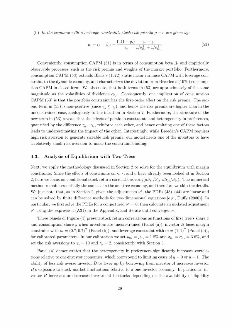
(ii) In the economy with a leverage constraint, stock risk premia µ− r are given by:

µt − rt = βCt − Γt(1− yt)γB

γB − γA1/σ2

D1 + 1/σ2D2

. (53)

Conveniently, consumption CAPM (51) is in terms of consumption beta βC and empiricallyobservable processes, such as the risk premia and weights of the market portfolio. Furthermore,consumption CAPM (53) extends Black’s (1972) static mean-variance CAPM with leverage con-straint to the dynamic economy, and characterizes the deviation from Breeden’s (1979) consump-tion CAPM in closed form. We also note, that both terms in (53) are approximately of the samemagnitude as the volatilities of dividends σDj . Consequently, one implication of consumptionCAPM (53) is that the portfolio constraint has the first-order effect on the risk premia. The sec-ond term in (53) is non-positive (since γA ≤ γB), and hence the risk premia are higher than in theunconstrained case, analogously to the intuition in Section 2. Furthermore, the structure of thenew term in (53) reveals that the effects of portfolio constraints and heterogeneity in preferences,quantified by the difference γB − γA, reinforce each other, and hence omitting one of these factorsleads to underestimating the impact of the other. Interestingly, while Breeden’s CAPM requireshigh risk aversion to generate sizeable risk premia, our model needs one of the investors to havea relatively small risk aversion to make the constraint binding.

4.3. Analysis of Equilibrium with Two Tress

Next, we apply the methodology discussed in Section 2 to solve for the equilibrium with marginconstraints. Since the effects of constraints on κ, r, and σ have already been looked at in Section2, here we focus on conditional stock return correlations corrt(dS1t/S1t, dS2t/S2t). The numericalmethod remains essentially the same as in the one-tree economy, and therefore we skip the details.We just note that, as in Section 2, given the adjustments ν∗, the PDEs (43)–(44) are linear andcan be solved by finite difference methods for two-dimensional equations [e.g., Duffy (2006)]. Inparticular, we first solve the PDEs for a conjectured ν∗ = 0, then calculate an updated adjustmentν∗ using the expression (A31) in the Appendix, and iterate until convergence.

Three panels of Figure (4) present stock return correlations as functions of first tree’s share xand consumption share y when investors are unconstrained (Panel (a)), investor B faces marginconstraint with m = (0.7, 0.7)> (Panel (b)), and leverage constraint with m = (1, 1)> (Panel (c)),for calibrated parameters. In our calibration we set µD1 = µD2 = 1.8% and σD1 = σD2 = 3.6%, andset the risk aversions to γA = 10 and γB = 2, consistently with Section 3.

Panel (a) demonstrates that the heterogeneity in preferences significantly increases correla-tions relative to one-investor economies, which correspond to limiting cases of y = 0 or y = 1. Theability of less risk averse investor B to lever up by borrowing from investor A increases investorB’s exposure to stock market fluctuations relative to a one-investor economy. In particular, in-vestor B increases or decreases investment in stocks depending on the availability of liquidity

29

00.1

0.20.3

0.40.5

0.60.7

0.80.9

1

00.10.20.30.40.50.60.70.8

x

(a) Stock Return Correlations, m = (0, 0)>

y

00.1

0.20.3

0.40.5

0.60.7

0.80.9

1

00.1

0.20.3

0.40.5

0.60.7

0.8

x

(b) Stock Return Correlations, m = (0.7, 0.7)>

y

00.1

0.20.3

0.40.5

0.60.7

0.80.9

1

00.1

0.20.3

0.40.5

0.60.7

0.8

x

(c) Stock Return Correlations, m = (1, 1)>

y

Figure 4: Conditional Stock Return Correlations.

Figure 4 presents the equilibrium stock return correlations when the investor is unconstrained (Panel(a)), faces margin constraint with m = (0.7, 0.7)> (Panel (b)), and leverage constraint with m = (1, 1)>(Panel (c)). Consumption share y = c∗B/D is countercyclical, and x = D1/D. The parameters are:µD1 = µD2 = 1.8%, σD1 = σD2 = 3.6%, ρ = 0.01, γA = 10, and γB = 2.

for borrowing. Moreover, the portfolio positions in both stocks tend to be adjusted in the samedirection in order to keep the portfolio diversified, which translates into higher correlations.

The increase in consumption share y of investor B has two opposing effects on the leverageeffect, which gives rise to a hump-shaped pattern on Panel (a). On one hand, this increase makesthe leverage effect more conspicuous by increasing the impact of the leveraged investor B on theeconomy, which pushes the correlations up. On the other hand, it reduces the consumption share1 − y of the lender A, and hence the availability of the liquidity for borrowing, which pushesthe correlations down. We further note that in the unconstrained case consumption share y ofinvestor B is procyclical in the sense that corrt(dyt, dDt) = 1. The procyclicality can be formallydemonstrated by noting that corrt(dyt, dDt) = −σ>ytσDt/(|σyt||σDt|), substituting volatility σyt

30

from (40), and setting ν∗ = 0. The intuition is the same as in Section 3.2.

Panel (a) demonstrates that, consistently with the empirical evidence [e.g., Ribeiro andVeronesi (2002)], stock return correlation is decreasing in y, and hence countercyclical, overa large interval. Panels (b) and (c) demonstrate that tighter constraints decrease correlations.Higher margins m1 and m2 reduce the ability of the less risk averse investor B to borrow, whichdecreases correlations, consistently with the intuition on the role of leverage.

Imposing the leverage constraint helps isolate and quantify the impact of leverage on corre-lations. The comparison of Panels (a) and (c), i.e., with and without borrowing, reveals that theleverage effect accounts for a significant fraction of the magnitude of correlations. Panel (c) thendemonstrates the impact of remaining effects on correlation, e.g. common discount factor effect,disentangled from the leverage effect. Panel (c) demonstrates that tight constraints give rise toa saddle-type pattern in correlations. In this case, the correlations appear to be higher when theeconomy is dominated by one tree, i.e. when share x is close to 0 or 1. Therefore, under portfolioconstraints the correlations crucially depend on the relative size x of a tree in the economy.

The two humps shown on Panel (c) are due to a combination of two effects that reinforceeach other. The first one is the common discount factor effect, which generates small humpseven in the unconstrained case on Panel (a). When x is close to 0 or 1, the state price densityξ is mainly driven by one tree. Consequently, irrespective of whether the dividend innovationsdD1 and dD2 move in the same or opposite directions, there will be extra comovement in stocks.When x is close to 0.5, ξ is less volatile since it is equally affected by both trees, and innovationsdD1 and dD2 may partially offset each other, which decreases the discount-driven comovement.

The second effect is specific to constraints, and plays no role in the unconstrained case. Weargue, that the leverage constraint homogenizes investors’ asset holdings more strongly aroundx = 0.5 than around x = 0 and x = 1, which leads to stronger decline in correlations aroundx = 0.5. When x = 0.5 both trees and stocks are “symmetric” since the trees have the samedrift and volatility parameters in the calibration. Therefore, in this case both stocks are equallyattractive to investors, and hence they invest equal fractions of wealth in stocks, i.e., θi1 = θi2. Inthe unconstrained case their asset holdings are still heterogeneous, since investor B can lever up.However, with leverage constraint, at x = 0.5 the shares of wealth invested in stocks have to bethe same: θ11 = θ12 = 0.5, and θ21 = θ22 = 0.5. Therefore, the constraint perfectly homogenizesasset holdings at x = 0.5. This is no longer the case when x is around 0 or 1, where stocks havedifferent riskiness and hence the portfolios remain different due to heterogeneity in risk aversions.

The intuition for the homogenization effect is similar to that in Section 3.2, where it wascaptured by equation (30). This intuition can be further verified by substituting ν∗σ−1m from(49) into the expression for σy in (40). Then, for the case σD1 = σD2 we obtain the followingexpression for σy, which quantifies the heterogeneity:

σyt = Γt(1− yt)(γB − γA)σD1

γAγB(x− 0.5, 0.5− x)>. (54)

Consistently with the intuition above, σy in equation (54) vanishes when x = 0.5. Hence, the

31

third term in volatilities σj , given by equation (42), which captures the impact of heterogeneityon volatilities, also vanishes, leading to the reduction in correlations.

5. Conclusion

We study the effects of portfolio constraints in one-tree and two-trees Lucas economies withheterogeneous CRRA investors. The previous literature widely employed the assumption ofmyopic logarithmic investors, which makes the characterization of equilibrium incomplete byeliminating the effects of constraints on wealth-consumption ratios of investors. Our modeldoes not rely on investor myopia, and hence provides a comprehensive analysis of the effects ofconstraints. In particular, we demonstrate under what conditions constraints increase or decreasestock return volatilities and price-dividend ratios, make them countercyclical or procyclical, andhelp quantitatively match market prices of risk and interest rates.

In one-tree economy we demonstrate that the limited participation constraint can generateequilibrium processes with dynamic characteristics consistent with empirical findings, and thatmargin constraints decrease stock return volatilities. In the economy with two trees we derivea generalization of Breeden’s (1979) consumption CAPM, which in the special case of lever-age constraints also generalizes Black’s (1972) static mean-variance CAPM. We also derive andstudy conditional stock return correlations in unconstrained and constrained economies. Wedemonstrate how the availability of liquidity in heterogeneous investor economy generates excesscorrelations, relative to homogeneous investor economies. We further demonstrate that tightermargin constraints decrease correlations by restricting investors’ ability to lever up.

Our model can be extended in various directions. In an ongoing work we study the impact ofconstraints in an economy with heterogeneous beliefs, where investors disagree on the aggregateconsumption growth in the economy. This setting allows to explore the impact of short-sale con-straints. Interesting direction for future research is the equilibrium with constrains in economieswhere investors are guided by Epstein-Zin recursive preferences, which help disentangle the effectsof risk aversion and the intertemporal elasticity of substitution.

32

Appendix A: Proofs

Proof of Proposition 1. To derive market price of risk κ and interest rate r we substituteoptimal consumptions (14) into consumption clearing condition in (8). Then, using dynamics(13) for state price densities in real and fictitious unconstrained economies, we apply Ito’s Lemmato both sides of consumption clearing condition, and by matching dt and dw terms obtain:

rt − ρΓt

− ytν∗t

γB+ 1

2(1 + γA

γ2A

(1− yt)κ2t + 1 + γB

γ2B

yt(κt + ν∗tm

σt

)2)= µD,

1− ytγA

κt + ytγB

(κt + ν∗tm

σt

)= σD.

(A1)

Solving equations (A1), we obtain κ and r in (17)–(18), where a1(y) and a2(y) are given by:

a1(yt) = Γ3tyt(1− yt)(γB − γA)

γ2Aγ

2B

, a2(yt) = −Γ3tyt(1− yt)

2γ2Aγ

2B

(1 + γAγB

Γt

). (A2)

The expressions (19)–(20) for the volatility σy and drift µy of consumption share y, which isconjectured to follow process (7), are obtained by applying Ito’s Lemma to yt = c∗B/Dt andmatching dt and dw terms. Stock return volatility σ is obtained by applying Ito’s Lemma toboth sides of S = ΨD, and matching dw terms.

To obtain ODEs (23)–(24), we first derive the HJB equations for investors’ value functionsJA and JB. The HJB equation for investor B in fictitious unconstrained economy is given byequation (15) in Remark 1, while the HJB equation for investor A is similar, but with ν∗ = 0, sinceinvestor A is unconstrained. Following Liu (2007) we conjecture that Ji = exp(−ρt)W 1−γiΦγi

i /(1−γi), where i = A,B. Then, the first order condition (F.O.C.) with respect to consumption,exp(−ρt)c−γii = ∂Ji/∂W , implies that Φi = ci/W , and hence Φi is the wealth-consumption ratio.The F.O.C. for portfolio weights gives the following expressions:

θ∗At = µt − rtγAσ2

t

− ytσytσt

Φ′A(yt)ΦA(yt)

, θ∗Bt = µt − rt + ν∗tmγBσ2

t

− ytσytσt

Φ′B(yt)ΦB(yt)

. (A3)

Next, as standard in the portfolio choice literature [e.g., Liu (2007)], substituting (A3) backinto HJB equations we obtain a PDE for the value function. Substituting conjectured Ji into thisPDE and cancelling like terms we obtain ODEs (23)–(24). Since the optimization problems aresolved in complete real and fictitious economies, the ODEs turn out to be linear, conditional onknowing the adjustment ν∗, consistently with Liu (2007). The adjustment ν∗ is derived in LemmaA.1 below. Finally, to derive Ψ, by summing up bond and stock market clearing conditions in (8)we obtain: W ∗A +W ∗B = S. The latter equation can be rewritten in terms of wealth-consumptionand price-dividend ratios as (1− y)ΦA + yΦB = Ψ. ¤

Lemma A.1. In a Markovian equilibrium the adjustment ν∗ and ratio m/σ are given by:

ν∗t =

1− b2tvtb1tv2

t

, if θ∗Btm = 1, ν∗t < 0,

0 , if θ∗Btm < 1,(A4)

33

m

σt=

vt , if θ∗Btm = 1, ν∗t < 0,m

σD

(1− Γtyt(1− yt)(γB − γA)

γAγB

Ψ′(yt)Ψ(yt)

) , if θ∗Btm < 1, (A5)

where b1, b2, v, and θ∗Bm are given by:

b1t = Γt(1− yt)γAγB

(1 + yt

Φ′B(yt)ΦB(yt)

), b2t = σD − (γB − γA)σDb1t, (A6)

vt = 1σD

+1 + yt

Φ′B(yt)ΦB(yt)

1 + ytΦ′B(yt)ΦB(yt)

− ytΨ′(yt)

Ψ(yt)

m− 1σD

, (A7)

θ∗Bm = b2tm

σt+ b1t

(mσt

)2ν∗t , (A8)

and wealth-consumption ratio is given by Ψ(y) = (1− y)ΦA(y) + yΦB(y).

Proof of Lemma A.1. The idea of the proof is to find adjustment ν∗ and ratio m/σ from asystem of two equations: the complementary slackness condition ν∗(θ∗Bm− 1) = 0 [e.g., Karatzasand Shreve (1998); Remark 1 in Section 2.1], and the equation form/σ derived from the expressionfor stock return volatility (21). Consider investor B who takes equilibrium processes as given.From portfolio constraint θ∗Bm ≤ 1, where θ∗B is given in (A3), we obtain an upper bound on ν∗:

ν∗t ≤(1− κt

γB

m

σt+ ytσyt

m

σt

Φ′B(yt)ΦB(yt)

) 11γB

(mσt

)2 . (A9)

Inequality (A9) is satisfied as an equality when the constraint is binding. Furthermore, Kuhn-Tucker condition implies ν∗ ≤ 0 [e.g., Karatzas and Shreve (1998); Remark 1 in Section 2.1].Moreover, since either the latter or the former inequalities should be satisfied as an equality,depending on whether the constraint is binding or not, we obtain:

ν∗t = min(

0; 1− κtγB

m

σt+ ytσyt

m

σt

Φ′B(yt)ΦB(yt)

) 11γB

(mσt

)2 . (A10)

Multiplying both sides of equation (21) for σ by m/σ, we obtain that m/σ satisfies equation:

m = m

σt

(σD − ytσytΨ

′(yt)Ψ(yt)

). (A11)

We observe that processes κ and σy depend on ν∗ in equilibrium. Substituting κ and σy from(17) and (19) into equations (A10) and (A11) we obtain two equations for ν∗ and m/σ, whichwe solve next. Also, substituting κ and σy from (17) and (19) into θ∗B in (A3) after some algebrawe obtain that θ∗Bm is given by (A8). When the constraint is binding, from equation (A10) or,equivalently, from equation θ∗Bm = 1, where θ∗Bm is given by (A8), after some algebra we obtain:

ν∗ = 1− b2t(m/σt)b1t(m/σt)2 , (A12)

34

where b1 and b2 are given by expressions (A6). When the constraint does not bind, i.e. θ∗Bm < 1,Kuhn-Tucker condition ν∗(θ∗Bm− 1) = 0 implies that ν∗ = 0. Consequently, we obtain:

ν∗t =

1− b2t(m/σt)b1t(m/σt)2 , if constraint binds,

0 , if constraint does not bind.(A13)

Next, we obtain an equation for m/σ, which together with equation (A13) gives a system ofequations for ν∗ and m/σ. Substituting σy from (19) into the equation for volatility σ in (21),and then multiplying both sides of the resulting equation by m/σ we obtain:

m = σD

(1− Γtyt(1− yt)(γB − γA)

γAγB

Ψ′(yt)Ψ(yt)

)m

σt+ Γt(1− yt)

γAγB

Ψ′(yt)Ψ(yt)

(mσt

)2ν∗t . (A14)

If the constraint does not bind, and hence ν∗ = 0, the second term in (A14) vanishes, and m/σ canbe easily found. If the constraint binds, substituting ν∗ from (A13) into equation (A14) yieldsa simple linear equation for m/σ from which we obtain expression (A5) for m/σ. Therefore,m/σ = v if the constraint binds, and hence from (A13) we obtain expression (A4) for ν∗.

We note, that the expressions in Lemma A.1 remain valid for the case of time-varying margins,e.g., m = m(yt, σt). If margin depends on volatility σ, the right-hand side of equation (A4) forν∗ depends on volatility σ via process v, given by (A7). To obtain ν∗ and σ in terms of Ψ, ΦBand their derivatives we note that ν∗ and σ solve the following system of two equations. Thefirst equation is the equation (A4) for ν∗, and the second equation is obtained by substitutingσy given by (19) into expression (21) for σ. This system can be solved in closed form in specialcases, e.g., when m(y, σ) is linear, and numerically when m(y, σ) is nonlinear. ¤

Proof of Proposition 2. In the unconstrained economy both investors have the same stateprice density, i.e., ξ = ξν∗ . Hence, from the expressions for optimal consumptions (14) we obtain:c−γAAt /c

−γBBt = λ, where λ is a constant. Consumption clearing implies: cAt + cBt = Dt. The latter

two equations imply that consumption share y = c∗B/D is given by

yt = f(λ− 1γAD

γB−γA

γA

t

), (A15)

where f(·) is an implicit function satisfying equation:

Zf(Z)γBγA + f(Z) = 1. (A16)

The s.p.d. in terms of consumption share is then given by:

ξt = λe−ρt(c∗Bt)−γB = λe−ρtf(λ− 1γAD

γB−γA

γA

t

)−γBD−γBt , (A17)

35

where λ is a constant. Consequently, the price-dividend ratio is given by:

Ψt = 1ξtEt[∫ +∞

t

ξτDτ

Dt

dτ]

=(Dt

c∗Bt

)−γBEt[∫ +∞

te−ρ(τ−t)

(Dτ

Dt

)1−γBf(Zt(Dτ

Dt

)γB−γAγA

)−γBdτ]

= yγBt Et

[∫ +∞

te−ρ(τ−t)

ητηtf(Zt(Dτ

Dt

)γB−γAγA

)−γBdτ],

(A18)

where Zt = λ−1/γAD(γB−γA)/γAt , ρ = ρ− (1− γB)µD + 0.5(1− γB)γBσ2

D, and ηt is a GBM martingale:

dηt = ηt(1− γB)σDdwt. (A19)

The third equality in (A18) uses the fact that Dt is a GBM, and hence it can be easily verified thatexp(−ρt)D1−γB

t = exp(−ρt)ηt. To facilitate tractability, we switch to new probability measureP with Radon-Nikodym derivative given by ητ/ηt, where η follows GBM process (A19). ByGirsanov’s Theorem, wt = wt − (1− γB)σDt is a Brownian motion under measure P.

We let E[·] denote the expectation under the new measure, rewrite expression (A18) underthe new measure, and then rewrite E[·] as an integral:

Ψt = yγBt Et

[∫ +∞

te−ρ(τ−t)f

(Zt(Dτ

Dt

)γB−γAγA

)−γBdτ]

= yγBt Et

[∫ +∞

te−ρ(τ−t)f

(Zte

q(τ−t)+√

Σ(wτ−wt))−γB

dτ]

= yγBt

∫ +∞

−∞

[∫ +∞

0

1√2πΣτ

e−(u−qτ)2

2Στ e−ρτf(Zte

u)−γB

dτ]du

= yγBt

∫ +∞

−∞

[∫ +∞

0

1√2πΣτ

e−(ρ+ q2

2Σ

)τ− u2

2Στ dτ]equΣ f(Zte

u)−γB

du

= yγBt√

2ρΣ + q2

∫ +∞

−∞eqΣu−√

2ρΣ+q2

Σ |u|f(Zte

u)−γB

du,

(A20)

where q = (γB − γA)(µD + 0.5(1 − 2γB)σ2D)/γA, Σ = (γB − γA)2σ2

D/γ2A , and similarly to Cochrane,

Longstaff, and Santa-Clara (2008) the inner integral in the fourth equality is computed usingformulas 3.471.9 and 8.469.3 in Gradshteyn and Ryzhik (2007).7

Next, we split the last integral in (A20) into two parts:

Ψt = yγBt

p

[ ∫ +∞

0eϕ−uf

(Zte

u)−γB

du+∫ 0

−∞eϕ+uf

(Zte

u)−γB

du], (A21)

7We use the following formula, implied by formulas 3.471.9 and 8.469.3 in Gradshteyn and Ryzhik (2007):∫ +∞

0

1√τe−aτ−

bτ dτ =

√π

ae−2√ab.

36

where constants p, ϕ− and ϕ+ are given by:

p =√

2ρΣ + q2, ϕ± = q ±√2ρΣ + q2

Σ , (A22)

and ρ = ρ−(1−γB)µD+0.5(1−γB)γBσ2D , q = (γB−γA)(µD+0.5(1−2γB)σ2

D)/γA, Σ = (γB−γA)2σ2D/γ

2A .

Our methodological contribution is to calculate the two integrals in (A21) using the changes ofvariable s = f(Zteu)/yt and s = (1− f(Zteu))/(1− yt), respectively, by observing from equation(A16) for f(Z) that inverse function f−1(y) is given by f−1(y) = (1− y)y−γB/γA .

To perform the change of variable s = f(Zteu)/yt in the first integral, we note that Zteu =f−1(yts) = (1 − yts)(yts)−γB/γA . Differentiating the last expression, and dividing both sides byZte

u we obtain:du = −

(γBγA

+(

1− γBγA

)yts

) 1s(1− yts)ds. (A23)

Next, we perform the change of variable. We also note, that since Zt = λ−1/γAD(γB−γA)/γAt ,

equations (A15)–(A16) imply that Zt = (1− yt)y−γB/γAt . After some algebra we obtain:8

I1 = yγBt

∫ +∞

0eϕ−uf

(Zte

u)−γB

du

=∫ 1

0

(1− yts)ϕ−−1

(1− yt)ϕ− s−γB−

γBγAϕ−−1

(γBγA

+(

1− γBγA

)yts

)ds

= −(1− yt)−ϕ−γA + ϕ−

2F1

(1− ϕ−,−γB −

γBγAϕ−, 1− γB −

γBγAϕ−; yt

)

+(

1− γBγA

)yt(1− yt)−ϕ−1− γB −

γBγAϕ−

2F1

(1− ϕ−, 1− γB −

γBγAϕ−, 2− γB −

γBγAϕ−; yt

),

(A24)

where 2F1(a, b, c; y) is a hypergeometric function [e.g., Gradshteyn and Ryzhik (2007)], given by:

2F1(a, b, c; y) = Γ(c)Γ(b)Γ(c− b)

∫ 1

0

sb−1(1− s)c−b−1

(1− ys)a ds.

Finally, we further simplify expression (A24) for integral I1 by using the following formula 9.131.1in Gradshteyn and Ryzhik (2007): 2F1(a, b, c; y)(1− y)a+b−c = 2F1(c− a, c− b, c; y). Then, alongthe same lines, we compute the second integral in (A21), and after some algebra we obtainexpression (26) for price-dividend ratio Ψ. ¤

Proof of Proposition 3. Similarly to Section 2, we embed the optimization of constrainedinvestor B into a fictitious complete-market economy, in which bonds and stocks follow dynamics:

dBt = Bt(rt + f(νt))dt, (A25)dSjt +Djtdt = = Sjt[(µjt + νjt + f(ν))dt+ σ>jtdwt], (A26)

8Bhamra and Uppal (2010) demonstrate how similar integrals can be evaluated using infinite series, and provideclosed-form expansions for price-dividend ratios and other equilibrium processes.

37

where ν = (ν1, ν2) ∈ R2, and f(ν) is the support function, given by:

f(ν) = supθ1m1+θ2m2≤1

(−ν1θ1 − ν2θ2), (A27)

where ν = (ν1, ν2)> are adjustments, proportional to Lagrange multipliers for constraints. Asdemonstrated in Karatzas and Shreve (1998), ν = (ν1, ν2)> ∈ Υ, where Υ is the effective domainfor f(ν), defined as Υ = ν ∈ R2 : f(ν) < +∞. Solving the optimization in (A27) we find thatΥ = ν = (m1,m2)>ν : ν ∈ R, ν ≤ 0. Noting the structure of effective domain Υ, we obtain:

νt = (m1,m2)>ν∗t , f(ν) = −ν∗t , (A28)

where ν∗ is such that ν∗ ≤ 0, and is derived in Lemma A.2 below. Similarly to Section 2.1, s.p.d.in the unconstrained real and fictitious economies, ξ and ξν∗ , follow dynamics:

dξt = −ξt[rtdt+ κ>t dwt], dξν∗t = −ξν∗t[(rt − ν∗t )dt+ (κt + ν∗t σ−1t m)>dwt]. (A29)

Similarly to Section 2.1, the optimal consumptions of investors A and B are given by equations(14). Substituting these consumptions into consumption clearing condition in (8), applying Ito’sLemma to both sides of (8), after matching the dt and dw terms we obtain that κ and r are givenby expressions (38)–(39), where a1(y) and a2(y) are given by (A2). We next derive expressions(40)–(41) for the volatility σy and drift µy of consumption share y by applying Ito’s Lemma toy = c∗B/D and matching dt and dw terms. The expressions (42) for volatilities σj are obtainedby applying Ito’s Lemma to both sides of Sj = ΨjDj and matching dw terms.

To obtain the PDEs for the price-dividend ratios Ψj(x, y) we apply Ito’s Lemma to both sidesof equation Ψj = Sj/Dj , and by matching dt terms we obtain:

12(x2σ>x σx

∂2Ψj

∂x2 − 2xyσ>y σx∂2Ψj

∂y∂x+ y2σ>y σy

∂2Ψj

∂x2

)+ xµx

∂Ψj

∂x− yµy ∂Ψj

∂y=

(−µDj + σ2Dj

+ µj − σDje>j σj)Ψj − e>j (x, 1− x), j = 1, 2,(A30)

where e1 = (1, 0)>, e2 = (0, 1)>. From the definition of the market price of risk κ = σ−1(µ− r),where µ− r = (µ1 − r, µ2 − r)>, we observe that µj = r + e>j σκ = r + σ>j κ. Next, we substituteµj = r + σ>j κ into the right-hand side of (A30), and then we replace σj by its expression (42) interms of derivatives of Ψj . After some algebra we then obtain PDEs (43).

The PDE for wealth-consumption ratio ΦB is obtained similarly to that in Section 2. Wefirst set up the HJB equation in the fictitious unconstrained economy. Following the portfoliochoice literature, e.g. Liu (2007), we conjecture that the value function takes the form JB =exp(−ρt)W 1−γBΦγB

B /(1−γB). Substituting this conjectured value function into the HJB after somealgebra, similarly to Liu (2007), we obtain PDE (44) which is linear in the fictitious complete-market economy if the adjustment ν∗ is known. To derive ΦA, by summing up bond and stockmarket clearing conditions in (8) we first obtain: W ∗A +W ∗B = S1 +S2. Then, we observe that thelatter equality after some algebra can be rewritten as (1− y)ΦA + yΦB = xΨ1 + (1− x)Ψ2, fromwhich we obtain ΦA. The adjustment parameter ν∗ is derived in the following Lemma A.2. ¤

38

Lemma A.2. In a Markovian equilibrium the adjustment ν∗ and vector σ−1m are given by:

ν∗t =

1− b>2tvtb1tv>t vt

, if m>θ∗Bt = 1, ν∗t < 0,

0 , if m>θ∗Bt < 1,(A31)

σ−1t m =

vt , if m>θ∗Bt = 1, ν∗t < 0,

(σt − (γB − γA)b3tσ>Dt)−1m , if m>θ∗Bt < 1,(A32)

where b1, b2, b3, σ, v, and m>θ∗B are given by:

b1t = Γt(1− yt)γAγB

(1 + ∂ΦBt

∂yt

ytΦBt

), b2t = σDt + σxt

∂ΦBt∂xt

xtΦBt− (γB − γA)σDtb1t, (A33)

b3t = Γt(1− yt)γAγB

(∂Ψ1t

∂yt

ytΨ1t

,∂Ψ2t

∂yt

ytΨ2t

)>, (A34)

σt =

σD1 0

0 σD2

+

(∂Ψ1t

∂xt

xtΨ1t

,∂Ψ2t

∂xt

xtΨ2t

)>σ>xt, (A35)

vt =( 1σD1

,1σD2

)>+Q−1(m1 − 1,m2 − 1)>, (A36)

m>θ∗Bt = b>2t(σ−1t m) + ν∗t b1t(σ−1

t m)>(σ−1t m), (A37)

and Q ∈ R2×2 is a matrix with elements Qjk given by:

(Qj1, Qj2)> = ejσDj + σxt∂Ψjt

∂xt

xtΨjt

− Γt(1− yt)γAγB

1b1t

(σDt + σxt

∂ΦBt∂xt

xtΦBt

)∂Ψjt

∂yt

ytΨjt

, (A38)

where j = 1, 2, e1 = (1, 0)> and e2 = (0, 1)>.

Proof of Lemma A.2. The idea of the proof is to demonstrate that ν∗ and σ−1m satisfy asystem of equations that can be solved in closed form in terms of ΦB, Ψj , and their derivatives.The first equation is the the complementary slackness condition ν∗(m>θ∗B −1) = 0 [e.g., Karatzasand Shreve (1998)], while the second is the equation for σ−1m which is derived from the expressionfor stock return volatilities in (42). First, we derive ν∗ as a function of σ−1m. It follows from thecomplementary slackness condition that ν∗ = 0, if the constraint does not bind. If the constraintbinds, ν∗ can be found from the condition m>θ∗B = 1, similarly to the proof of Lemma A.1.

In the fictitious complete-market economy with s.p.d. following (A29) the optimal θ∗B can befound in terms of wealth-consumption ratio ΦB in the same way as in complete-market portfoliochoice literature [e.g., Liu (2007)], and is given by:

θ∗Bt = (σ>t )−1(κt + ν∗t σ

−1t m

γB+ σxt

∂ΦBt∂xt

xtΦBt− σyt ∂ΦBt

∂yt

ytΦBt

), (A39)

where κ+ν∗σ−1m is the market price of risk in the fictitious unconstrained economy. Substitutingκ from (38) and σy from (40) into θ∗B in (A39), after some algebra we obtain expression for m>θ∗B

39

in (A37). Then, proceeding exactly as in the proof of Lemma A.1, we obtain:

ν∗t =

1− b>2t(σ−1t m)

b1t(σ−1t m)>σ−1

t m, if constraint binds,

0 , if constraint does not bind.(A40)

Next, we derive an equation for σ−1m in terms of ν∗. First, we substitute volatility σy from(40) into volatility σj in (42), which yields volatility matrix σ in terms of adjustment ν∗:

σt = σt − (γB − γA)b3tσ>Dt + ν∗t b3t(σ−1t m)>, (A41)

where vector b3 ∈ R2 and matrix σ ∈ R2×2 are given by (A34) and (A35), respectively. Multi-plying both sides of equation (A41) by σ−1

t m from the left, we obtain:

m = σtσ−1t m− (γB − γA)b3tσ>Dtσ−1

t m+ ν∗t b3t(σ−1t m)>σ−1

t m. (A42)

The adjustment ν∗ and vector σ−1m satisfy the system of equations (A40) and (A42), whichwe next solve in closed form. When the constraint is binding, ν∗ is given by the expression in thefirst line of (A40). Substituting this expression into equation (A42) we obtain a linear equationfor σ−1m, which has the following solution:

σ−1t m = Q−1(m− b3t/b1t), (A43)

where Q ∈ R2×2 is a matrix with elements given by (A38). To simplify the solution in (A43)we note that vector v∗ = (1/σD1 , 1/σD2)> solves equation Qv∗ = 1 − b3/b1. This result can beverified by multiplying matrix Q and vector v∗, and using an easily verifiable fact that σ>D v∗ = 1and σ>x v

∗ = 0, where σD = (xσD1 , (1 − x)σD2)> and σx = ((1 − x)σD1 ,−(1 − x)σD2)> are definedin (32) and (37). Substituting b3/b1 = 1 − Qv∗ into (A43) we obtain σ−1m = (1/σD1 , 1/σD2)> +Q−1(m1 − 1,m2 − 1)>. Similarly, when the constraint does not bind, and hence ν∗ = 0, (A42)becomes a linear equation for σ−1m, which can be solved in closed form. Consequently, we obtainexpression (A32) for vector σ−1m. Then, denoting v = σ−1m for the case when the constraintbinds, we obtain expression (A32) for vector σ−1m. ¤

40

Proof of Proposition 4.

(i) We now prove the first part of the Proposition. Similarly to the proof of Proposition 2,consumption share y and s.p.d. ξ are given by (A15) and (A17), respectively, where f(·) isan implicit function satisfying equation (A16). Analogously to the proof of Proposition 2, theprice-dividend ratio for the first stock is given by:

Ψ1t = 1D1t(c∗Bt)−γB

Et[∫ +∞

te−ρ(τ−t)D1τD

−γBτ f

(λ− 1γAD

γB−γA

γA

τ

)−γBdτ]

= 1D1t(c∗Bt)−γB

Et[∫ +∞

te−ρ(τ−t)D1−γB

1τ

(1 + D2τ

D1τ

)−γBf(λ− 1γAD

γB−γA

γA

1τ

(1 + D2τ

D1τ

)γB−γAγA

)−γBdτ]

=( ytxt

)γBEt[∫ +∞

te−ρ(τ−t)

ητηt

(1 + D2τ

D1τ

)−γBf(λ− 1γAD

γB−γA

γA

1τ

(1 + D2τ

D1τ

)γB−γAγA

)−γBdτ]

=( ytxt

)γBEt[∫ +∞

te−ρ(τ−t)

(1 + D2τ

D1τ

)−γBf(λ− 1γAD

γB−γA

γA

1τ

(1 + D2τ

D1τ

)γB−γAγA

)−γBdτ],

(A44)where ρ = ρ− (1− γB)µD1 + 0.5(1− γB)γBσ2

D1 , ηt is a GBM martingale:

dηt = ηt(1− γB)σD1dw1t,

and E[·] is the expectation under a new measure P that has ητ/ηt as its Radon-Nikodym derivative.

Next, rewriting the processes for D1 and D2 in (32) under the new measure, we obtain:

λ− 1γAD

γB−γA

γA

1τ = λ− 1γAD

γB−γA

γA

1t eu1 ,D2τ

D1τ= D1t

D2teu2 , (A45)

where u = (u1, u2)> has distribution N(q(τ − t),Σ(τ − t)), q and Σ are given by:

q =(γB − γA

γA(µD1 + 0.5(1− 2γB)σ2

D1), µD2 − µD1 + 0.5(2γB − 1)σ2D1 − 0.5σ2

D2

)>,

Σ =

(γB−γAγA

)2σ2D1 −

γB−γAγA

σ2D1

−γB−γAγA

σ2D1 σ2

D1 + σ2D2

(A46)

Next, we also define parameter p as follows:

p =√

2(ρ− (1− γB)µD1 + 0.5(1− γB)γBσ2

D1

)+ q>Σ−1q. (A47)

Rewriting the expectation in (A44) as a double integral involving p.d.f. of the joint normal

41

distribution N(q(τ − t),Σ(τ − t)), we obtain:

Ψ1t =( ytxt

)γB ∫ +∞

−∞

∫ +∞

−∞

(1 + D2t

D1teu2)−γB

f(λ− 1γAD

γB−γA

γA

1t eu1(1 + D2t

D1teu2)γB−γA

γA

)−γB×

12π√

det(Σ)

[∫ +∞

0

1τe−ρτ−

12τ (u−qτ)>Σ−1(u−qτ)dτ

]du1 du2,

=( ytxt

)γB ∫ +∞

−∞

∫ +∞

−∞

(1 + D2t

D1teu2)−γB

f(λ− 1γAD

γB−γA

γA

1t eu1(1 + D2t

D1teu2)γB−γA

γA

)−γB×

eq>Σ−1uK0(p

√u>Σ−1u)

π√

det(Σ)du1 du2,

(A48)

where the last equality is computed using integral 3.471.9 in Gradshteyn and Ryzhik (2007), andK0(·) is McDonald’s function, given in closed form by integral 8.432.1 in Gradshteyn and Ryzhik(2007) and also implemented in Matlab.9

To eliminate function f(·) from equation (A48) we perform the following change of variables:

z = f(λ− 1γAD

γB−γA

γA

1t eu1(1 + D2t

D1teu2)γB−γA

γA

), s =

(1 + D2t

D1teu2)−1

(A49)

From equation (A16) we observe that f−1(z) = (1− z)z−γB/γA . Furthermore, from the definitionof share x = D1/D we note that D2/D1 = (1− x)/x, and from equation for share y in (A15) weobtain λ−1/γAD

(γB−γA)/γA1 = f−1(y)/x(γA−γB)/γA = (1 − y)y−γB/γA/x(γA−γB)/γA . Using these expres-

sions, we solve equations (A49), and obtain u1 and u2 as functions of s, z, x, and y given by (48).Finally, computing the partial derivatives of u1 and u2 in (48) w.r.t. s and z we obtain:

du1 du2 =

∣∣∣∣∣∣∂u1/∂z ∂u1/∂s

∂u2/∂z ∂u2/∂s

∣∣∣∣∣∣ds dz = γB(1− z) + γAz

γAs(1− s)z(1− z) ds dz. (A50)

Using the expression for du1du2 in (A50), after performing the change of variables, we obtainprice-dividend ratio Ψ1(x, y) in (47). The expression for Ψ2(x, y) can be derived analogously.

(ii) We now prove the second part of Proposition 4. When the leverage constraint is binding,substituting m1 = 1 and m2 = 1 into expression (A32) we find that σ−1m = (1/σD1 , 1/σD2)>.Next, we observe that the following easily verifiable equalities hold:

σ>Dt(1/σD1 , 1/σD2)> = 1, σ>xt(1/σD1 , 1/σD2)> = 0, (A51)

where σDt =(xtσD1 , (1− xt)σD1

)>and σxt =

((1− xt)σD1 ,−(1− xt)σD2

)are defined in (32) and

(37). Substituting σ−1m into the expression for ν∗ in (A40), using equalities (A51) we obtain the9Integrals 3.471.9 and 8.432.1 in Gradshteyn and Ryzhik (2007) imply that

∫ +∞

0

1τe−aτ−

bτ dτ = 2K0(2

√ab), K0(z) =

∫ +∞

0e−z cosh(s)ds.

42

expression for ν∗ in (49). Using equalities (A51) one more time, we find that portfolio constraintis satisfied as an equality for all x and y, i.e., (1, 1)>θ∗B = 1. Intuitively, the constraint is identicallybinding since B always wants to borrow, but is prevented by constraints.

Then, we derive closed-form expressions for Ψj , j = 1, 2. Consider the ratio of marginalutilities: λt = (c∗At)−γA/(c∗Bt)−γB . From the F.O.C. in (14) we obtain that λt = λξt/ξν∗t, where λis a constant, and ξt and ξν∗t follow processes (A29). Applying Ito’s Lemma to λt we obtain:

dλt = −λt[ν∗t(1−m>(σ>t )−1(κt + ν∗t σ

−1t m)

)dt− (ν∗t σ−1

t m)> dwt]. (A52)

Substituting κt from (38), σ−1m = (1/σD1 , 1/σD2)>, and ν∗ from (49) into process (A52), we findthat λt follows a GBM:

dλt = λtγB − γA

1/σ2D1 + 1/σ2

D2

[(γB − 1)dt+

( 1σD1

,1σD2

)>dwt

]. (A53)

Similarly to the proof of the first part of Proposition 4, the consumption share of constrainedinvestor B is given by yt = f(λ−1/γA

t D(γB−γA)/γAt ), where f(·) solves equation (A16). The dividends

should be priced using s.p.d. ξt, where from F.O.C. (14) for unconstrained investor A ξt =(1/ψA)e−ρt((1− yt)Dt)−γA . Then, proceeding similarly as in the unconstrained case, we obtain:10

Ψ1t =(1− yt

xt

)γAEt[∫ ∞t

e−ρ(τ−t)(1 + D2τ

D1τ

)−γA(1− f(λ− 1γA

τ D

γB−γA

γA

1τ

(1 + D2τ

D1τ

)γB−γAγA

))−γAdτ],

(A54)where ρ = ρ − (1 − γA)µD1 + 0.5(1 − γA)γAσ2

D1 , and E[·] is an expectation under new measure P,such that wt = wt − (1− γA)σD1t is a Brownian motion under P. From the fact that λt, D1t andD2t follow GBMs (A53) and (32), respectively, we obtain:

λ− 1γA

τ D

γB−γA

γA

1τ = λ− 1γA

t D

γB−γA

γA

1t ed11(τ−t)+d12εt√τ−t,

D2τ

D1τ= D2t

D1ted21(τ−t)+d22εt

√τ−t, (A55)

where εt =(−σD1(w1τ − w1t) + σD2(w2τ − w2t)

)/√

(σ2D1 + σ2

D2)(τ − t) ∼ N(0, 1), and

d11 = γB − γAγA

(µD1 + 1− 2γA

2 σ2D1

)− (γB − γA)2

2γA1

1/σ2D1 + 1/σ2

D2

, d12 = −γB − γAγA

σ2D1√

σ2D1 + σ2

D2

,

d21 = µD2 − µD1 − 0.5σ2D2 −

1− 2γA2 σ2

D1 , d22 =√σ2D1 + σ2

D2 .

(A56)

Finally, similarly to the unconstrained case, we rewrite the expectation operator in equation(A54) as an integral w.r.t. εt, and change variables ε and τ − t to the following ones:

z = f(λ− 1γA

t D

γB−γA

γA

1t ed11(τ−t)+d12εt√τ−t(1 + D2t

D1ted21(τ−t)+d22εt

√τ−t)γB−γA

γA

),

s =(1 + D2t

D1ted21(τ−t)+d22εt

√τ−t)−1

.

(A57)

10Since the equilibrium processes are given in closed form, are uniformly bounded and continuous, and theprocess for λt follows a GBM, it can be verified that ξtS1t +

∫ t0 ξτD1τdτ is a martingale, there are no endogenous

bubbles in the economy, and the price-dividend ratio is given by “present value” formula (A54).

43

After the change of variables in equation (A57), similarly to the unconstrained case, we obtain:

Ψ1t =∫ 1

0

∫ 1

0

( sx

1− y1− z

)γA γB(1− z) + γAz

z(1− z)s(1− s)F (s, z;x, y) ds dz, (A58)

where

F (s, z;x, y) =

e−ρτ(s,z;x,y)−0.5ε(x,y)2/τ(s,z;x,y)

γA|d11d22 − d12d21|√

2πτ(s, z;x, y), τ(s, z;x, y) > 0,

0, τ(s, z;x, y) ≤ 0,(A59)

ρ = ρ− (1− γA)µD1 + 0.5(1− γA)γAσ2D1 , ε(x, y) and τ(x, y) are given by:

ε(s, z;x, y) = 1d12d21 − d11d22

[d21

(ln(1− z

1− y)− γBγA

ln(zy

)+ γB − γA

γAln( sx

))− d11 ln

( 1− s1− x

x

s

)],

τ(s, z;x, y) = 1d11d22 − d12d21

[d22

(ln(1− z

1− y)− γBγA

ln(zy

)+ γB − γA

γAln( sx

))− d12 ln

( 1− s1− x

x

s

)],

and dij are given by expressions (A56). Price-dividend ratio Ψ2t is found analogously. ¤

Proof of Corollary 1.

(i) The risk premium of the market portfolio is given by µM − r = θ>M (µ− r). Multiplying bothsides of the equation for excess returns (50) by θM we obtain:

µM − r = θMβC − ΓtytγB

ν∗θ>Mm. (A60)

Next, from equation (A60) we find multiplier (Γy/γB)ν∗ in terms of µM−r, and after substitutingthis multiplier back into equation (50) we obtain consumption CAPM (51).

(ii) Consumption CAPM (53) is derived by substituting ν∗ given by (49) into equation (50). ¤

44

Appendix B: Numerical Method

In this Appendix we first discuss in greater details how to obtain boundary conditions for ODEs(23)–(24). In particular, we derive the boundary conditions for the case of limited participation(i.e., m > 1), which is less tractable than the case of margin constraints (i.e., m < 1) discussedin Section 2.3. We also present an alternative way of dealing with boundary conditions. Then,we discuss the finite difference method, its numerical accuracy, and the speed of convergence.Finally, we discuss how our numerical approach is modified in the case of two trees.

B.1. Boundary Conditions

In this subsection we provide detailed derivations of boundary conditions at y = 1 for the case oflimited participation, while the case of margin constraints is analogous. At y = 0 the conditionsare the same as in Section 2.3. We remark here, that an alternative way of dealing with boundaryconditions is to derive ODEs for functions Φi(y) = y(1− y)Φi, which have boundary conditionsΦi(0) = Φi(1) = 0, provided that Φi is sufficiently smooth at the boundaries (see discussionbelow). We check that this approach works equally well with proper boundary conditions. Theonly disadvantage of this approach is that it does not provide insights on the boundary behaviorof solutions, which motivates us to look for proper boundary conditions.

In contrast to the case of margin constraints, in the case of limited participation the limity → 1 does not correspond to a homogeneous-investor economy populated by investor B only.The reason is that in such an economy investor B is constrained to hold θ∗B = 1/m < 1, whichviolates market clearing in stocks. Consequently, the state y = 1 is repulsive in a sense that it isnever reached, and consumption share y is repulsed back after approaching 1 too closely. As aresult, the boundary condition at y = 1 is not given by a wealth-consumption ratio in a limitingeconomy. Instead, as demonstrated below, this condition captures the admissible rate of changein wealth-consumption ratio ΦB when the economy approaches y = 1.

We assume that Φi(y) ∈ C1[0, 1] and are smooth enough at the boundaries, so that

limy→1

(1− y)Φ′′A (y) = 0, limy→1

(1− y)Φ′′B (y) = 0. (B1)

After computing the equilibrium via finite difference method with a very fine grid of ten thousandpoints we check conditions (B1) numerically. We find that they are satisfied for the case of marginrequirements when m < 1, and for the case of restricted participation when m > 1 and γi > 1.When m > 1 and γi < 1 the numerical analysis shows that assumptions (B1) are violated, inwhich case, to deal with boundary conditions we solve for smoother functions Φi(y) = y(1−y)Φi,and then infer Φi. Lemma B.1 summarizes our result.

Lemma B.1. If conditions (B1) are satisfied, the boundary conditions at y = 1 in the case oflimited participation with m > 1 are given by:

(γA − 1)ΦA(1) = 0, (γB − 1)ΦB(1) = Φ′B(1), (B2)

45

while boundary conditions at y = 0 are the same as in equations (27).

Proof of Lemma B.1. First, we derive boundary conditions assuming that

limy→1

ν∗(y) = l1, limy→1

(1− y)ν∗(y)v(y) = l2, (B3)

where l1 and l2 are non-zero constants, and then show that assumptions (B3) are indeed satisfied.The adjustment ν∗ and v are given by equations (A4) and (A7), respectively, and we recall thatby definition v = m/σ when the constraint is binding. We also note that the constraint has tobe binding around y = 1, since investor B is less risk averse. Below we provide the analysis forΦB, while the derivation for ΦA is analogous.

We write down ODE (24) for ΦB around y = 1, substitute κ from (17) and v = m/σ, andafter multiplying this ODE by 1− y we obtain:

y2σ2y

2 (1 − y)Φ′′B − y(1− y)(µy + 1− γB

γBγA

(ΓγAσD + (1− y)ν∗vΓ

)σy)Φ′B

+ (1− y)(1− γB

2γBγ2A

(ΓγAσD + (1− y)ν∗vΓ

)2+ (1− γB)(r − ν∗)− ρ

)ΦBγB

+ 1− y = 0,(B4)

Expression (19) for σy, assumptions (B1) and (B3) imply that the first term in (B4) converges tozero in the limit. Similarly, using expressions (17)–(20) for equilibrium parameters we eliminateother terms that converge to zero, and obtain:

(limy→1

(1− y)rγB

)Φ′B(1) +

(limy→1

(1− y)rγB

)(1− γB)ΦB(1) = 0, (B5)

where (1 − y)r/γB comes from µy in equation (B4), which is given by (20). It turns out that(1 − y)r does not converge to zero due to term a2(y)(ν∗m/σ)2 in the expression for r in (18),where function a2(y) is given by (A2). Indeed, from the expression for a2(y) we obtain that(1 − y)a2(y)ν∗(m/σ)2 ∼ (1 − y)2(ν∗v)2, which converges to a non-zero limit in accordance withassumption (B3). Canceling like terms in (B5) we obtain the boundary condition for ΦB.

Now it remains to prove assumptions (B3). Substituting ν∗ and v from (A4) and (A7) into(B3), after taking the limit we obtain:

limy→1

(1− y)ν∗(y)v(y) = limy→1

(1− y)1− b2(y)v(y)b1(y)v(y) = −γAσD,

limy→1

(1− y)v(y) =1 + Φ′B(1)

ΦB(1)[1 + yt

Φ′B(yt)ΦB(yt)

− ytΨ′(yt)

Ψ(yt)

]′

y=1

m− 1σD

,

(B6)

where the last limit uses the fact that 1+yΦ′B(y)/ΦB(y)−yΨ′(y)/Ψ(y)→ 0, which can be verifiedby substituting Ψ = (1 − y)ΦA + yΦB. It can be shown that the derivative of the expression insquare brackets in (B6), evaluated at y = 1, is non-zero. The limits in (B6) imply (B3). ¤

46

B.2. Finite Difference Method

Now, we turn to the computation of equilibrium. One way of computing the equilibrium is byfixed-point iterations. Namely, we conjecture ODE (23)–(24) solutions, and calculate ν∗, andequilibrium processes κ, r, σy, µy, σ. Then, we solve the ODEs again, with updated coefficients,find new solutions, and iterate the process until convergence. The second way is to fix largehorizon T , find the differential equations for a model with finite horizon and then solve the modelbackwards until reaching a time-independent solution [e.g., Ljungqvist and Sargent (2004)].

Below, we argue that the second approach adds stability to the numerical algorithm but haslower speed of convergence. We use the fixed point iterations method to solve for the equilibriawith margin constraints when m < 1, and use the combination of the two methods for the limitedparticipation m ≥ 1 where the performance of fixed point method deteriorates unless the initialconjecture is close enough to the actual equilibrium. Each step of our algorithms reduces tosolving a system of linear equations.

For simplicity, we omit subscript i. Next, we fix horizon T , denote the time and state variableincrements by ∆t ≡ T/M and ∆y ≡ 1/N , respectively, where M and N are integer numbers,and index time and state variables by t = 0,∆t, 2∆t, ..., T and y = 0,∆y, 2∆y, ..., 1, respectively.Then, we derive the following discrete-time analogues of ODEs (23)–(24) and boundary conditionsby replacing derivatives with their finite-difference analogues:

dΦn,k+1 − Φn,k

∆t + an,k+1Φn+1,k − 2Φn,k + Φn−1,k

∆y2 + bn,k+1Φn+1,k − Φn−1,k

2∆y+ cn,k+1Φn,k + 1 = 0,

(B7)

Φn,M = hn, Φ0,k = e0,k, ΦN,k = eN,kΦN−1,k + eN,k, (B8)

where n = 1, 2, ..., N − 1, k = 1, 2, ...,M − 1, Φn,k = Φ(n∆y, k∆t). The coefficients in (B7)correspond to coefficients in ODEs (23)–(24) and are computed using the solution Φn,k+1 froma preceding step, while coefficients in (B8) are obtained by replacing terminal and boundaryconditions at y = 0 and y = 1 by their finite-difference analogues. Parameter d in (B7) specifiesthe solution method. The cases d = 0 and d = 1 correspond to pure fixed point and backwardsin time iterations, respectively, while 0 < d < 1 describes a method in between. The system ofequations in (B7)–(B8) is solved backwards, starting at k = M − 1. Step-k coefficients in (B7)are computed using step-(k + 1) solution Φn,k+1, and hence step-k function Φn,k solves a systemof linear algebraic equations for fixed k. We then iterate until convergence.

When d = 0, the first term in (B7) vanishes, and the resulting numerical scheme becomes animplicit finite-differences scheme for ODEs (23)–(24), where k indexes the iteration. If d = 1, thefirst term in equation (B7) corresponds to ∂Φ(y, t)/∂t, which is a standard term in finite-horizonHJB equations. The algorithms with and without the first term in (B7) converge to the sameresult. However, sometimes methods with 0 < d ≤ 1 improve performance for the followingreason. For a fixed k system of linear equations (B7) is a system with a three-diagonal matrix.Numerical methods with such matrices are known to be more stable when the absolute values of

47

the elements on the main diagonal exceed the sum of the absolute values of elements on upperand lower diagonals. It can be shown that the first term in (B7) increases the absolute value ofthe elements on the main diagonal, and hence increases the computational stability.

The convergence is assessed by computing the maximum weighted difference between wealth-consumption ratios 10 years (or iterations, when d = 0) apart: ε1 = 0.5 max

y|ΦB(y, t)− ΦB(y, t+

10)|+0.5 maxy|ΦA(y, t)−ΦA(y, t+10)|. In the backwards iterations case we also looked at another

measure given by ε2 = 0.5 maxy|(ΦB(y, t)−ΦB(y, t+∆t))/∆t|+0.5 max

y|(ΦA(y, t)−ΦA(y, t+∆t))/∆t|.

We solve the model setting N = 1000 and for both convergence measures get typical precisionsaround ε ∼ 10−9 after a couple of seconds of Matlab calculations on a PC. We also cross-checkthe numerical and closed-form solutions, where possible.

Our methodology remains the same for solving the model with two trees. We use the methodof iterations, described above, and at each point in time solve a system of linear algebraic equa-tions. However, the problem becomes more computationally intensive since PDEs for wealth-consumption and price-dividend ratios are two-dimensional. We solve PDEs using fine-differencesmethod, which involves solving a system of linear algebraic equations with matrix Ω given by:

Ω =

Ωc,1 Ωu,1 0 0 . . . 0 0 0Ωl,2 Ωc,2 Ωu,2 0 . . . 0 0 0

0 Ωl,3 Ωc,3 Ωu,3 . . . 0 0 0. . . . . . . . . . . . . . . . . . . . . . . .

0 0 0 0 0 Ωl,N−2 Ωc,N−2 Ωu,N−2

0 0 0 0 0 0 Ωl,N−1 Ωc,N−1

,

where elements Ωl,n, Ωc,n, and Ωu,n are (N − 1)× (N − 1) three-diagonal matrices, and N is thenumber of grid points. The number of grid points is the same for x ∈ [0, 1] and y ∈ [0, 1]. Forsimplicity of dealing with boundary conditions we solve for functions Φ = x(1 − x)y(1 − y)Φ,which have zero boundary conditions, and then recover function Φ. Other computational aspectsof the algorithm remain the same as for the one-dimensional case.

48

Appendix C: Verification of Optimality

In this Appendix we derive easily verifiable sufficient conditions of optimality. The investorssolve their optimization problem taking equilibrium processes as given. Consequently, the verifi-cation of optimality is studied holding these processes fixed. Our dynamic programming solutionapproach allows us to provide the verification results by employing the techniques available inthe literature [e.g., Fleming and Soner (2005)], modified to take into account Kuhn-Tucker con-ditions. Our results also justify the conjectured functional form of the value function, that weused to derive ODEs (23)–(24) for wealth-consumption ratios.

For brevity, we consider only the optimization of constrained investor B, and hence restrictourselves to considering portfolio weights that satisfy investor’s portfolio constraint. We considerself-financing admissible consumption and portfolio strategies ct and θt, such that

∣∣∣Et[∫ +∞

t

c1−γBτ

1− γBdτ]∣∣∣ < +∞, |θt|m ≤ 1. (C1)

We also note, that in the economy with margin constraints (i.e., m < 1), these constraints neverbind for investor A in equilibrium. Hence, margin constraints, and conditions (C1), can beimposed on investor A without loss of generality. Lemma C.1 below summarizes our results.

Lemma C.1 (Verification of Optimality). Let ΦB(yt) be a twice continuously differentiablesolution of ODE (24). Suppose, that |σt| < C1, |(µt + ν∗t − rt)/σt| < C1, where C1 is a constant,and consider function JB(Wt, yt, t), given by:

JB(Wt, yt, t) = W1−γBt ΦB(yt)γB

1− γB. (C2)

(i) Let strategies ct and θt be such that conditions (C1) are satisfied, and

Et[∫ T

0JB(Wτ , yτ , τ)2dτ

]< +∞, for all T > 0, (C3)

lim supT→+∞

Et[JB(WT , yT , T )] ≥ 0, (C4)

where Wτ is wealth, generated by strategies ct and θt. Then, the following inequality holds:

JB(Wt, yt, t) ≥ Et[∫ +∞

0

c1−γBτ

1− γBdτ]. (C5)

(ii) Suppose, that 0 < ΦB(y) ≤ C1. Then, c∗t = Wt/ΦB(yt) and θ∗Bt in (A3) are optimal, and

JB(Wt, yt, t) = Et[∫ +∞

0

(c∗τ )1−γB

1− γBdτ]. (C6)

49

The proof of Lemma C.1 is given below, and is similar to the proofs of verification theoremsin the literature [e.g., Fleming and Soner (2005)]. We also note that condition (C4) is triviallysatisfied when 0 < γB < 1, since in this case value function (C2) is positive. This condition is ananalogue of terminal conditions in finite-horizon models, and is widely employed in the literature[e.g., Fleming and Soner (2005)]. We also require volatility σ and adjusted market price ofrisk (µ + ν∗ − r)/σ to be bounded, and wealth-consumption ratio ΦB to be twice continuouslydifferentiable, which can be verified numerically.

In particular, in the case of margin constraints, studied in Section 3.2, it can be shownthat price-dividend ratio ΦA(y), volatility σ, market price of risk κ, and adjustment ν∗ are allcontinuous and bounded functions. Similarly, using very fine grid, we check that derivativesΦ′B(y) and Φ′′B (y) also appear to be continuous. Consequently, Lemma C.1 applies to the caseof margin constraints. In the case of limited participation in Section 3.1, market price of risk κis unbounded, and hence this case requires a more subtle verification theorem, which is beyondour scope. We only note that one potential way of obtaining a more powerful verification resultmight be to determine the asymptotic rate of growth of equilibrium processes near y = 1, and todemonstrate that the singularity at this point is integrable.

Proof of Lemma C.1.

(i) First, we construct the following process:

Ut =t∫

0

c1−γBτ

1− γBdτ + JB(Wt, yt, t). (C7)

Next, we derive a stochastic differential equation (SDE) for Ut in the following form:

dUt = Ut[µUtdt+ σUtdwt]. (C8)

By applying Ito’s Lemma to process (C7), adding and subtracting ν∗(θtm − 1)W∂JB/∂W fromthe drift, we find that µU and σU are given by:

µUt = 1Ut

(e−ρt

c1−γBt

1− γB+ ∂JBt

∂t+[Wt

(rt − ν∗t + θt(µt − rt + ν∗tm)

)− ct

]∂JBt∂Wt

−ytµyt∂JBt∂yt

+ 12[W 2t θ

2tσ

2t

∂2JBt∂W 2

t

− 2Wtθtσtytσyt∂2JBt∂Wt∂yt

+ y2t σ

2yt

∂2JBt∂y2

t

])

−ν∗(θtm− 1)

UtWt

∂JBt∂Wt

.

(C9)

σUt = JtUt

((1− γB)θtσt − γBytσyt

Φ′B(y)ΦB(y)

)

= JtUt

((1− γB)θtσt + γBθ

∗Btσt −

µt − rt + ν∗tσt

),

(C10)

50

where the second equality in (C10) is derived by expressing yσyΦ′B(y)/ΦB(y) in terms of θ∗B and(µ−r+ν∗)/σ from the expression for portfolio weight θ∗B in (A3). We note that the first componentof µU is non-positive because JBt satisfies HJB equation (15) with “max” operator, while the firstterm in (C9) is evaluated at a sub-optimal strategy (c, θ). The second term in (C9) is non-positivebecause ν∗ ≤ 0, θtm− 1 ≤ 0 by assumption (C1), and ∂JB/∂Wt ≥ 0. Consequently, µU ≤ 0.

From conditions (C1) and (C3) it follows that Et[∫ T

0 (UτσUτ )2dτ ] < +∞, and hence we obtainthat Et[

∫ T0 UτσUτdwτ ]=0, for all T . Consequently, integrating SDE (C8) from t to T , and taking

expectations on both sides, we find that Ut ≥ Et[UT ], which can be rewritten as follows:

JB(Wt, yt, t) ≥ Et[∫ T

t

c1−γBτ

1− γBdτ]

+ Et[JB(WT , yT , T )

]. (C11)

From condition (C4) it follows that there exists a subsequence Tn such that limEt[J(WTn , yTn , Tn)] ≥0, as n→∞. We also note that

∫ Tnt c

1−γBτ /(1− γB)dτ is a monotone sequence of random variables,

and hence its limit can be calculated using monotone convergence theorem [Shiryaev (1996)].Consequently, taking the limit in (C11) we obtain inequality (C5).

(ii) First, we demonstrate that transversality condition Et[JB(WT , yT , T )]→ 0 is satisfied as T → 0,where wealth WT is under strategies c∗ and θ∗. To this end, we apply Ito’s Lemma to JB(Wt, yt, t).Then, we add and subtract e−ρt(c∗Bt)1−γB/(1− γB) and ν∗(θ∗Btm− 1)Wt∂JBt/∂Wt in the drift termof the process, taking into account condition ν∗(θ∗Btm− 1) = 0. Noting that JB(Wt, yt, t) satisfiesHJB equation (15) we obtain:

dJBt = JBt[µJtdt+ σJtdtwt], (C12)

where drift µJ and volatility σJ are given by:

µJt = −e−ρt (c∗Bt)1−γB

1− γB1JBt

, σJt = (1− γB)θ∗Btσt − γBytσytΦ′B(y)ΦB(y) . (C13)

From the F.O.C. for consumption we obtain that e−ρt(c∗B)1−γB/(1− γB) = JB/ΦB(y), and fromthe expression for the optimal portfolio weight (A3) we obtain that yσyΦ′B(y)/ΦB(y) = (µ − r +ν∗)/σ − γBθ∗Bσ. Substituting these expressions back into expressions (C13), we obtain:

µJt = − 1ΦB(y) , σJt = θ∗Bt −

µt − rt + ν∗tσt

. (C14)

By assumptions of Lemma 4 σJ satisfies Novikov’s condition, and hence process dηt = ηtσJtdwt isan exponential martingale. Using the martingality of ηt from (C12) and (C14) we obtain:

|Et[J(WT , yT , T )]| = Et[ 1|1− γB|

exp(−∫ T

t

1ΦB(yτ )dτ

)ηTηt

]

≤ e−(T−t)/C1

|1− γB|Et[ηTηt

]= e−(T−t)/C1

|1− γB|.

(C15)

From inequality (C15) it easily follows that Et[J(WT , yT , T )]→ 0, as T →∞.

51

Next, we consider the following process:

U∗t =t∫

0

c∗τ1−γB

1− γBdτ + JB(Wt, yt, t). (C16)

Applying Ito’s Lemma to process U∗t we find its drift and volatility. We note, that the drift isgiven by expression (C9) evaluated at ct = c∗t , and θt = θ∗Bt. Substituting c∗t and θ∗Bt into thisexpression, from the fact that JBt satisfies HJB equation (15) and the complementary slacknesscondition ν∗(θ∗Btm− 1)=0 we observe that drift (C9) is zero. Consequently, U∗t follows a process:

dU∗t = U∗tJBtU∗t

(θ∗Bt −

µt − rt + ν∗tσt

)dwt. (C17)

Since 0 < JBt/U∗t < 1, and given the assumptions of Lemma 4, the volatility of process U∗t satisfies

Novikov’s condition, and hence U∗t is an exponential martingale. Consequently, integrating (C17)from t to T and taking the expectations on both sides, after some algebra we obtain:

JB(Wt, yt, t) = Et[∫ T

t

(c∗τ )1−γB

1− γBdτ]

+ Et[JB(WT , yT , T )

]. (C18)

Next, we pass to the limit T → +∞ in (C18). In the limit, the last term in (C18) vanishes dueto inequality (C15), while the first term converges to (C6) by monotone convergence theorem. ¤

52

ReferencesAbel, A., 2002, “An Exploration of the Effects of Pessimism and Doubt on Asset Returns,”

Journal of Economic Dynamics and Control, 26, 1075-1092.Basak, S., 2000, “A Model of Dynamic Equilibrium Asset Pricing with Heterogeneous Beliefs

and Extraneous Risk,” Journal of Economic Dynamics and Control, 24, 63-95.Basak, S., 2005, “Asset Pricing with Heterogeneous Beliefs,” Journal of Banking and Finance,

29, 2849-2881.Basak, S., and B. Croitoru, 2000, “Equilibrium Mispricing in a Capital Market with Portfolio

Constraints,” Review of Financial Studies, 13, 715-748.Basak, S., and B. Croitoru, 2006, “On the Role of Arbitrageurs in Rational Markets,” Journal

of Financial Economics, 81, 143-173.Basak, S., and D. Cuoco, 1998, “An Equilibrium Model with Restricted Stock Market Partici-

pation,” Review of Financial Studies, 11, 309-341.Bhamra, H.S., and R. Uppal, 2009, “The Effect of Introducing a Non-Redundant Derivative on

the Volatility of Stock-Market Returns When Agents Differ in Risk Aversion,” Review ofFinancial Studies, 22, 2303-2330.

Bhamra, H.S., and R. Uppal, 2010, “Asset Prices with Heterogeneity in Preferences and Beliefs,”Working Paper, University of British Columbia.

Black, F., 1972, “Capital Market Equilibrium with Restricted Borrowing,” Journal of Business,45, 444-455.

Breeden, D.T., 1979, “An Intertemporal Asset Pricing Model with Stochastic Consumption andInvestment Opportunities,” Journal of Financial Economics, 7, 265-296.

Brunnermeier, M.K., and L.H. Pedersen, 2008, “Market Liquidity and Funding Liquidity,” Re-view of Financial Studies, 22, 2201-2238.

Buraschi, A., P. Porchia, and F. Trojani, 2010, “Correlation Risk and Optimal Portfolio Choice,”Journal of Finance, 65, 393-420.

Buraschi, A., F. Trojani, and A. Vedolin, 2010, “When Uncertainty Blows in the Orchard:Comovement and Equilibrium Volatility Risk Premia,” Working Paper, Imperial CollegeLondon.

Buss, A., and B. Dumas, 2012, “The Equilibrium Dynamics of Liquidity and Illiquid AssetPrices,” Working Paper, INSEAD.

Campbell, J.Y., 2003, “Consumption-Based Asset Pricing,” Handbook of Economics and Fi-nance, G. Constantinides, M. Harris, and R. Stulz (eds.), Amsterdam: North Holland.

Campbell, J.Y., 2006, “Household Finance,” Journal of Finance, 61, 1553-1604.Campbell, J.Y., and J.H. Cochrane, 1999, “By Force of Habit: A Consumption-Based Expla-

nation of Aggregate Stock Market Behavior,” Journal of Political Economy, 107, 205-251.Campbell, J.Y., and R.J. Shiller, 1988, “The Dividend-Price Ratio and Expectations of Future

Dividends and Discount Factors,” Review of Financial Studies, 3, 195-227.Chabakauri, G., 2009, “Asset Pricing in General Equilibrium with Constraints,” Working Paper,

London School of Economics.Chan, Y.L., and L. Kogan, 2002, “Catching Up with the Joneses: Heterogeneous Preferences

and the Dynamics of Asset Prices,” Journal of Political Economy, 110, 1255-1285.

53

Chen, H., and S. Joslin, 2011, “Generalized Transform Analysis of Affine Processes and Appli-cations in finance,” Review of Financial Studies, forthcoming.

Chien, Y., H. Cole, and H. Lustig, 2011, “A Multiplier Approach to Understanding the MacroImplications of Household Finance,” Review of Economic Studies, 78, 199-234.

Cochrane, J.H., F.A. Longstaff, and P. Santa-Clara, 2008, “Two Trees,” Review of FinancialStudies, 21, 347-385.

Coen-Pirani, D., 2005, “Margin Requirements and Equilibrium Asset Prices,” Journal of Mon-etary Economics, 52, 449-475.

Colacito, R., and M.M. Croce, 2012, “International Robust Disagreement,” American EconomicReview, 102, 152-155.

Cuoco, D., 1997, “Optimal Consumption and Equilibrium Prices with Portfolio Constraints andStochastic Income,” Journal of Economic Theory, 72, 33-73.

Cuoco, D., and H. He, 2001, “Dynamic Aggregation and Computation of Equilibria in Finite-Dimensional Economies with Incomplete Markets,” Annals of Economics and Finance, 2,265-296.

Cvitanic, J., and I. Karatzas, 1992, “Convex Duality in Constrained Portfolio Optimization,”Annals of Applied Probability, 2, 767-818.

Cvitanic, J., and S. Malamud, 2011, “Price Impact and Portfolio Impact,” Journal of FinancialEconomics, 100, 201-225.

Danielsson, J., H. Shin, and J.P. Zigrand, 2009, “Risk Appetite and Endogenous Risk,” WorkingPaper, London School of Economics.

Detemple, J.B., and S. Murthy, 1997, “Equilibrium Asset Prices and No-Arbitrage with PortfolioConstraints,” Review of Financial Studies, 10, 1133-1174.

Detemple, J.B., R. Garcia, and M. Rindisbacher, 2003, “A Monte-Carlo Method for OptimalPortfolios,” Journal of Finance, 58, 401-446.

Detemple, J.B., and M. Rindisbacher, 2005, “Closed-Form Solutions for Optimal Portfolio Se-lection with Stochastic Interest Rate and Investment Constraints,” Mathematical Finance,15, 539-568.

Driessen, J., P. Maenhout, and G. Vilkov, 2009, “The Price of Correlation Risk: Evidence fromEquity Options,” Journal of Finance, 64, 1377-1406.

Duffie, D., 2001, Dynamic Asset Pricing Theory, Princeton, NJ: Princeton University Press.Duffy, 2006, Finite Difference Methods in Financial Engineering, Chichester, England: John

Wiley and Sons.Dumas, B., 1989, “Two-Person Dynamic Equilibrium in the Capital Market,” Review of Finan-

cial Studies, 2, 157-188.Dumas, B., and A. Lyasoff, 2012, “Incomplete-Market Equilibria Solved Recursively on an Event

Tree,” Journal of Finance, forthcoming.Dumas, B., and P. Maenhout, 2002, “A Central-Planning Approach to Dynamic Incomplete-

Market Equilibrium,” Working Paper, INSEAD.Ehling, P., and C. Heyerdahl-Larsen, 2012, “Correlations,” Working Paper, London business

School.Ferson, W.E, and C.R. Harvey, 1991, “The Variation of Economic Risk Premiums,” Journal of

Political Economy, 99, 385-415.

54

Fleming, W.H., and H.M. Soner, 2005, Controlled Markov Processes and Viscosity Solutions,New York: Springer.

Fostel, A., and J. Geanakoplos, 2008, “Leverage Cycles and Anxious Economy”, AmericanEconomic Review, 98, 1211-1244.

Gallmeyer, M., and B. Hollifield, 2008, “An Examination of Heterogeneous Beliefs with a Short-Sale Constraint in a Dynamic Equilibrium,” Review of Finance, 12, 323-364.

Garleanu, N., and S. Panageas, 2010, “Young, Old, Conservative, and Bold: The Implications ofHeterogeneity and Finite Lives for Asset Pricing,” Working Paper, University of California,Berkeley.

Garleanu, N., and L.H. Pedersen, 2011, “Margin Based Asset Pricing and the Deviations fromthe Law of One Price,” Review of Financial Studies, 1980-2022.

Geanakoplos, J., 2009, “The Leverage Cycle,” NBER Macroeconomic Annual.Gomes, F., and A. Michaelides, 2008, “Asset Pricing with Limited Risk Sharing and Heteroge-

neous Agents,” Review of Financial Studies, 21, 416-448.Gradshteyn, I.S., and I.M. Ryzhik, 2000, Table of Integrals, Series, and Products (6th ed.), New

York: Academic Press.Gromb, D., and D. Vayanos, 2002, “Equilibrium and Welfare in Markets with Financially Con-

strained Arbitrageurs,” Journal of Financial Economics, 66, 361-407.Gromb, D., and D. Vayanos, 2009, “Financially Constrained Arbitrage and Cross-Market Con-

tagion,” Working Paper, INSEAD.Gromb, D., and D. Vayanos, 2010, “Limits of Arbitrage: The State of the Theory,” Annual

Review of Financial Economics, 2, 251-275.Guvenen, F., 2006, “Reconciling Conflicting Evidence on the Elasticity of Intertemporal Sub-

stitution: A Macroeconomic Perspective,” Journal of Monetary Economics, 53, 1451-1472.Guvenen, F., 2009, “A Parsimonious Macroeconomic Model for Asset Pricing,” Econometrica,

77, 1711-1750.Hardouvelis, G.A., and P. Theodossiou, 2002, “The Asymmetric Relation Between Initial Mar-

gin Requirements and Stock Market Volatility Across Bull and Bear Markets,” Review ofFinancial Studies, 15, 1525-1559.

Hansen, L., and T. Sargent, 2007, Robustness, Princeton, NJ: Princeton University Press.He, Z., and A. Krishnamurthy, 2011, “A Model of Capital and Crises,” Review of Economic

Studies, forthcoming.Heaton, J., and D.J. Lucas, 1996, “Evaluating the Effects of incomplete Markets on Risk Sharing

and Asset Pricing,” Journal of Political Economy, 104, 443-487.Huang, C.-F., and H. Pages, 1992, “Optimal Consumption and Portfolio Policies with an Infinite

Horizon: Existence and Convergence,” Annals of Applied Probability, 2, 36-64.Hugonnier, J., 2012, “Rational Asset Pricing Bubbles and Portfolio Constraints,” Journal of

Economic Theory, forthcoming.Karatzas, I., and S.E. Shreve, 1998, Methods of Mathematical Finance, New York: Springer-

Verlag.Kogan, L., I. Makarov, and R. Uppal, 2007, “The Equity Premium and the Riskfree Rate in an

Economy with Borrowing Constraints,” Mathematics and Financial Economics, 1, 1-19.

55

Liu, J., 2007, “Portfolio Selection in Stochastic Environments,” Review of Financial Studies,20, 1-39.

Ljungqvist, L., and T.J. Sargent, 2004, Recursive Macroeconomic Theory, Cambridge: MITPress.

Longstaff, F.A., 2009, “Portfolio Claustrophobia: Asset Pricing in Markets with Illiquid Assets,”American Economic Review, 99, 1119-1144.

Longstaff, F.A., and J. Wang, 2008, “Asset Pricing and Credit Markets,” Working Paper, UCLA.Lucas, R.E., 1978, “Asset Prices in an Exchange Economy”, Econometrica, 46, 1429-1445.Mankiw, N.G., and S.P. Zeldes, 1991, “The Consumption of Stockholders and Non-stockholders,”

Journal of Financial Economics, 29, 97-112.Martin, I., 2011, “The Lucas Orchard,” Working Paper, Stanford University.Mas-Colell, A., M. Whinston, and J.R. Green, 1995, Microeconomic Theory, Oxford, UK: Ox-

ford University Press.Mehra, R., and E.C. Prescott, 1985, “The Equity Premium: A Puzzle,” Journal of Monetary

Economics, 15, 145-161.Menzly, L., T. Santos, and P. Veronesi, 2004, “Understanding Predictability,” Journal of Polit-

ical Economy, 112, 1-47.Pavlova, A., and R. Rigobon, 2008, “The Role of Portfolio Constraints in the International

Propagation of Shocks,” Review of Economic Studies, 75, 1215-1256.Prieto, R., 2010, “Dynamic Equilibrium with Heterogeneous Agents and Risk Constraints,”

Working Paper, Boston University.Ribeiro, R., and P. Veronesi, 2002, “The Excess Comovement of International Stock Markets in

bad Times: A Rational Expectations Equilibrium Model,” Working Paper, University ofChicago.

Rytchkov, O., 2009. “Dynamic Margin Constraints,” Working Paper, Temple University.Samuelson, W., and R. Zeckhouser, 1988, “Status Quo Bias in Decision Making,” Journal of

Risk and Uncertainty, 1, 7-59.Santos, T., and P. Veronesi, 2006, “Labor Income and Predictable Stock Returns,” Review of

Financial Studies, 19, 1-44.Schornick, A.V., 2009, “Competing Capital Constraints,” Working Paper, INSEAD.Schwert, W., 1989, “Why Does Stock Market Volatility Change Over Time?” Journal of Fi-

nance, 44, 1115-1153.Shapiro, A., 2002, “The Investor Recognition Hypothesis in a Dynamic General Equilibrium:

Theory and Evidence,” Review of Financial Studies, 15, 97-141.Shiller, R.J., 1981, “Do Stock Prices Move Too Much to be Justified by Subsequent Changes in

Dividends?” American Economic Review, 71, 421-436.Shiryaev, A.N., 1996, Probability, New York: Springer.Srinivas, P.S., E. Whitehouse, and J. Yermo, 2000, “Regulating Private Pension Funds’ Struc-

ture, Performance and Investments: Cross-Country Evidence,” Working Paper, WorldBank.

Wu, T., 2008, “An Equilibrium Model with Buy and Hold Investors”, Working Paper, IllinoisInstitute of Technology.

56