Asset price booms and monetary policy

This version 26 January

Carsten Detken and Frank Smets*

AbstractThe paper aims at deriving some stylised facts for financial, real, and monetary policy developments

during asset price booms by means of aggregating information contained in 38 boom periods since the

1970s for 18 OECD countries. We observe 26 macroeconomic variables in a pre-boom, boom and

post-boom phase. Not all booms lead to large output losses. We divide our sample in high-cost and

low-cost booms and analyse the differences. High-cost booms are clearly those in which real estate

prices and investment crash in the post-boom periods. In general it is difficult to distinguish a high-

cost from a low-cost boom at an early stage. However, high-cost booms seem to follow very rapid

growth in the real money and real credit stocks just before the boom and at the early stages of a boom.

During high-cost booms, rates of change of real estate prices and consumption growth are significantly

higher and the investment (especially housing) GDP ratio deviation from trend rises faster over the

whole boom period. There is also evidence that high-cost booms are associated with significantly

looser monetary policy conditions over the boom period, especially towards the late stage of a boom.

We finally discuss the results with regard to the theoretical literature. The looser monetary policy at

the later stage of high-cost booms could be interpreted in different ways. It could be that excessively

loose monetary policy contributes to extending the boom and exacerbating the real and financial

imbalances. Alternatively, observed monetary policy could reflect a desirable, pre-emptive loosening

in anticipation of an asset price crash to come.

JEL classification system: E44, E52, E58

Keywords: asset price booms, asset price bubbles, optimal monetary policy, over-investment, real

estate prices

* European Central Bank. E-mail: Carsten.Detken@ecb.int and Frank.Smets@ecb.int. The views expressed are

solely our own and do not necessarily reflect those of the European Central Bank. We thank our discussants

Gerhard Illing and Peter Sellin and Kiel Week, 23-24 June 2003 conference participants and ECB Workshop,

11-12 December 2003 participants for valuable comments. We particularly thank Ramon Adalid for excellent

research assistance.

2

Non-technical summary

We characterise financial, real and monetary policy developments during asset price booms

aggregating information contained in 38 boom periods since the 1970s for 18 OECD countries. We

observe 26 variables in a pre-boom, boom and post-boom phase. An asset price boom is defined as a

positive deviation of an aggregate asset price indicator from its recursively estimated trend by at least

10 percent. The asset price indicator aggregates equity, private and commercial real estate prices

according to the respective weights in the economy. It turns out that both equity and real estate prices

rise strongly during the boom and crash in the post boom period. Real GDP growth is particularly

strong during the boom, which is mainly driven by total private investment and is also reflected in

housing investment, in both cases both in terms of growth rates as well as gaps (i.e. the deviation of

the ratio to GDP from trend). Monetary policy is looser during boom periods than in normal times as

is revealed by deviations from the Taylor rule, as well as money and credit conditions.

Not all asset price booms lead to a bust and not all busts to a financial crisis. Therefore we divide our

sample of boom episodes into high- and low-cost booms, depending on the relative post-boom growth

performance. This classification criterium thus focuses on the volatility of real GDP growth over the

whole boom and post-boom phase. We test which variables allow discriminating between high- and

low-cost booms. The clearest and most significant differences between high- and low-cost booms can

be found for the post-boom period. Real estate prices, and gaps, investment growth, housing

investment growth and gaps, just to name a few, drop significantly more in post-high-cost boom

periods. At the same time inflation gaps are significantly higher, monetary policy significantly looser

(as measured by deviations from a Taylor rule) and reductions in real money growth and gaps and real

credit growth and gaps significantly larger in post-high-cost boom periods.

There are fewer significant differences during boom periods. During high-cost booms, for example,

real estate prices rise stronger, the output gap improves more, real monetary and real credit growth is

larger and there is some evidence that monetary policy is loosened more. The stronger loosening of

monetary policy rather seems to be a passive monetary policy choice, as interest rates simply do not

rise sufficiently to neutralise the rising output and inflation gaps. A possible explanation is that

monetary policy authorities are uncertain about the cause of the asset price boom - productivity

induced or non-fundamental - and are therefore reluctant to act in a determined way. Another

explanation would be that towards late stages of the boom, central banks perceive to be trapped

between price stability and asset price (or rather investment-) stability and are reluctant to actively

trade-off one against the other. A third possibility is that the loosening of monetary policy with respect

to the Taylor rule towards the end of high-cost booms is a deliberate and desirable policy. It could be

that, depending on the stochastic properties of the asset price bubble, the optimal policy corresponds

exactly to the observed initial tightening and later relaxation of the monetary policy stance as the

boom proceeds. The loosening is supposed to be desirable due to lags in the transmission mechanism

3

of monetary policy, so that a pre-emptive accommodation of the anticipated asset price crash becomes

optimal.

High cost booms also last on average one half to one year longer than low-cost booms and lead to an

about 3.5 percentage points larger deviation from the aggregate asset price trend. Unfortunately we

find only few significant differences in the pre-boom year, which would be most useful from a policy

maker’s perspective. What stands out is the higher real money growth in high-cost pre-boom periods

and higher real credit growth in the first year of booms. Neither of these two facts can be explained by

simple business cycle developments.

Our search for stylised facts with regard to asset price boom episodes, by construction, cannot say

much about the role of monetary policy in responding or even triggering asset price booms. Monetary

policy is clearly endogenous so that the issue of causality is not addressed. If anything, one would be

tempted to argue that low inflation is probably not related to high-cost booms, which instead rather

seem to be associated with too loose monetary policy.

We supplement the empirical analysis by a survey of the theoretical literature concerning optimal

monetary policy in times of asset price booms. To illustrate the difficulties involved in deriving clear-

cut conclusions, we finally present simulated optimal policy reactions to show how the monetary

policy response depends on the nature of the underlying shock responsible for the asset price increase.

4

1. Introduction

Following a long bull market and the exuberance associated with the new economy boom of the

1990s, stock market indices have fallen sharply and persistently over the past two to three years.

Historically, asset price crashes have often been associated with sharp declines in economic activity

and financial instability. Large falls in asset prices can not only have substantial wealth effects on

consumption. They also reduce collateral values, which may lead to cuts in bank lending, thereby

exacerbating the fall in spending and leading to further knock-on effects on asset prices, lending and

economic activity. While since the start of the new millennium many industrial countries have

experienced economic slowdowns as stock prices have fallen, the current downturns have not been

particularly severe and the financial sector has been quite resilient. One possible factor is that in many

countries house prices have continued to rise. Nevertheless, policy makers have come under pressure

for not having responded earlier to the build-up of the asset price boom, thereby possibly preventing or

alleviating the subsequent bust and its effects on economic activity and inflation.1

In this paper we address a number of monetary policy issues associated with the occurrence of large

asset price booms and busts. The paper has two objectives. First, we want to characterise the real and

financial developments surrounding asset price booms. Following the recent work by Borio and Lowe

(2001), Helbling and Terrones (2003), Bordo and Jeanne (2002a, 2002b) and Mishkin and White

(2003), we identify asset price booms since the early 1970s and characterise what happens during the

boom, just before and immediately following it. We define asset price booms as a period in which

aggregate (i.e. weighted equity, commercial and private real estate) real asset prices are more than 10

percent above their recursively estimated Hodrick Prescott trend2. In light of the discussion above, our

focus is on the behaviour of monetary policy during those booms as captured by changes in short-term

interest rates, money and credit aggregates and deviations from Taylor rules. We make a distinction

between those booms that were followed by a large recession and those that were not and compare the

characteristic features – including the monetary policy response.

We find that the average length of aggregate asset price booms in the eighteen industrial countries we

study has increased from 1.3 years in the 1970s to 3.5 years in the 1980s and 4.4 years in the 1990s.

Their occurrence is, however, not uniform across countries. Asset price booms are typically associated

with a substantial increase in the output gap and the investment and housing investment/GDP ratio

relative to the respective trends. Moreover, these booms are supported by relatively easy monetary

conditions, as captured by low interest rates relative to a Taylor rule benchmark, and abundant

monetary and credit conditions as indicated by rising money and credit gaps as well as high money

1 See, for example, Greenspan (2002).2 Our methodology is similar although not equal to Gourinchas et al. (2001) application to lending booms.

5

and credit growth rates. In contrast, considering all booms, inflation rates do not move very much

during the boom, although inflation deviations from trend rise during the boom. The booms that were

followed by a large recession, and in some cases financial instability, are typically longer, give rise to

significantly greater real and monetary imbalances, and, in particular, are characterised by a big boom

and bust in real estate markets. High-cost booms are also characterised by a more positive inflation

gap, i.e. a larger deviation from the inflation trend, following the boom, in spite of the large drop in

output and investment.

Second, in light of this historical experience, we then review the theoretical literature on how central

banks should respond to such asset price booms. Should central banks have responded earlier to the

boom in order to reduce the size of the bust and its effects? Should central banks be more aggressive

in responding to the downward phase than they normally would have done? Four different strands of

the literature can be distinguished. The early work of Bernanke and Gertler (1999, 2001) and Cechetti

et al (2000) focused on whether it was useful to include a response to asset prices in addition to the

response to an inflation forecast. Dupor (2001, 2002) analyses the trade-off that may arise between

price stability and asset price stabilisation when there are frictions in the credit market and non-

fundamental shocks in asset markets. Borio and Lowe (2002) and Bordo and Jeanne (2002b) focus on

the implications of the non-linearities that may arise as financial imbalances increase the probability of

a self-fulfilling bust in collateral values and credit, possibly leading to financial fragility. Finally, a

small number of papers have focused on the incentive and moral hasard effects that may arise when a

central bank responds too aggressively to an asset price collapse (e.g. Caballero and Krishnamurthy,

2003; Illing, 2001; Miller et al. 2000).

The literature review highlights that the optimal monetary policy response is not necessarily easy to

characterise. As shown in Smets (1997) and Dupor (2002), the optimal response very much depends

on the underlying source of the asset price increase. In particular, the direction of the policy response

may be different depending on whether asset prices are driven by improved productivity or over-

optimistic expectations. Given the uncertainty surrounding estimates of equilibrium values of asset

prices, such an assessment of the sources of the shocks will in general not be an easy task. As

discussed in Dupor (2001) and illustrated in this paper with the model of Smets and Wouters (2003),

non-fundamental asset price shocks may introduce a trade off between inflation stabilisation and asset

price stabilisation. However, compared to cost-push shocks, the time inconsistency problem would

appear to be much less as such shocks will typically tend to move the output gap and inflation in the

same direction. A characterisation of optimal monetary policy becomes even more complicated when

one allows for the probability that a rise in financial imbalances may results in a financial crisis with

large negative effects on economic activity and price stability. As shown in Bordo and Jeanne (2002b),

the optimality of a pre-emptive tightening of policy will then depend on a careful assessment of the

6

probability of a bubble emerging and an estimate of the costs of such pre-emptive action. Our

empirical results may be seen as consistent with recent findings that the build-up of large real,

financial and monetary imbalances may provide a good indicator of problems to come (e.g. Borio and

Lowe 2002). However, whether a more pre-emptive tightening than historically observed would have

been successful in preventing or alleviating the subsequent asset price collapse without imposing too

high a cost remains a question for research. Finally, we believe more research needs to be done on the

incentive and moral hasard effects of a reactive policy approach, whereby the central bank only

responds when the asset price collapse occurs. To the extent that such an approach provides implicit

insurance to the private agents against large asset price collapses, it may ex ante lead to larger run-up

in financial imbalances and increase the vulnerability of the private sector to asset market shocks.

2. Asset price booms and monetary policy: the stylised facts

In this section we describe the average development of financial, real and monetary policy indicators

around aggregate asset price boom episodes. In the following, we first lay out the methodology for

identifying asset price booms. Then we analyse how on average the economy evolved before, during

and following the asset price booms with a focus on monetary conditions. Finally, we distinguish

between those booms that were followed by a collapse in output growth and those that were not. We

attempt to identify the different characteristics between those two types of booms.

2.1 Methodology

In order to identify asset price booms we use the BIS data set on aggregate real asset prices. In this

data set an aggregate real asset price index is computed as a weighted average of real equity prices and

real residential and commercial real estate prices, where the weights are based on the relative share of

those assets in the private sector’s wealth.3 We define an asset price boom as a period in which the

aggregate real asset price index is continuously more than 10% above its trend.4 The trend is

calculated recursively using a one-sided Hodrick-Prescott filter with a smoothing parameter of 1000.5

Following Borio and Lowe (2002), we use the asset price gap rather than its growth rate to define a

boom. This allows to stress the concept of accumulated financial imbalances, e.g. reducing the weight

of periods of rapid asset price growth directly following an asset price collapse. It also allows for

sustained periods of asset price growth only slightly above trend to generate a boom as imbalances can

accumulate.

3 For a description of how the aggregate real asset price index is constructed, see Borio, Kennedy and Prowse

(1994) and Borio and Lowe (2002).4 Many thanks to Steve Arthur and Claudio Borio from the BIS for providing us their data set.5 The lambda parameter is the same as in Gourinchas et al. (2001). See the data annex for a short discussion.

7

We are aware of the fact that the HP filter on average is too close to the data towards the sample end.

By choosing a λ of 1000 we let the trend only adjust very smoothly and introduce a phase shift of the

trend. The advantage is that the resulting boom periods start later than with a traditional trough to peak

method but earlier than a gap deviation from an ex-post trend (due to the phase shift). Our booms

could theoretically end after the peak, as long as the deviation from trend is still high enough but

would finish typically before a boom identified by an ex-post trend gap. This method in combination

with the threshold value of 10% gives very reasonable results, see figure A in the annex. Furthermore

it has the advantage that it can be computed in “real” time, i.e. as soon as data for the current year are

available. The recursive HP filter is similar to a moving average characterisation of the trend and is

thus resembling chartist methods used in financial market. This has the additional advantage that our

method might capture booms the way they were perceived at the time. Correcting the problems of the

HP filter at the current end by using forecasts (see e.g. Kaiser and Maravall, 1999) would be counter-

productive as first of all, it is exactly the phase shift that allows for a very reasonable timing of the

boom and second, good forecasts for asset prices are impossible to obtain with simple univariate

forecasting models (or in fact any other model).

Borio and Lowe (2002) have shown that deviations from trend (in particular applied to credit) are

relatively good predictors of financial instability. One consequence of our boom definition is that

different asset price booms can be of different length. In order to be able to compare financial and

economic developments in different asset price booms, we therefore calculate the average annual

growth rate during the boom as well as the change over the whole boom period. The pre-boom period

is defined as the two years before the asset price boom, while the post-boom period is defined as the

two years following the boom.

Table A1 in the appendix lists each of the 38 aggregate asset price booms that we identify in this way.

Figure A in the appendix plots in the left graph the real aggregate asset price index, the recursively

estimated HP trend and indicates the asset price boom periods as shaded areas. It is also mentioned

whether the boom is classified as high (H) or low(L)-cost, as will be explained below. The right chart

repeats the real aggregate asset price index but also shows two of its three components, i.e. real

residential property prices and real equity prices. We find boom episodes in every country, although

they are not equally spread over each of the 18 countries considered. It is interesting to note that less

than five boom years each are found in the three largest countries of the euro area (Germany, France

and Italy) as well as in Belgium and Canada. In contrast 10 or more boom years spread over two or

three distinct periods are detected in Finland, Ireland, the Netherlands, and the United Kingdom. Over

the whole sample, the average length of the asset price booms is somewhat greater than three years.

This hides, however, a lot of variation across asset price booms. The longest successive boom period

identified in this data set lasts for nine years. It is the asset price boom in Finland from 1981 till 1989.

8

In addition, there are three additional successive boom periods lasting for 6 years or longer (Spain:

1986-1991; Ireland: 1995-2001; the Netherlands: 1994-2001). There is a tendency of the asset price

booms to become longer. The average length increases from 1.3 years in the 1970s to 3.5 years in the

1980s and 4.4 years in the 1990s. However, most of the boom episodes took place in the second half

of the 1980s and early 1990s (18 compared to 9 in the 1970s/early 1980s and 11 in the late 1990s/early

2000). In this context, it is worth noting that one factor which may have contributed to the larger

number of asset price booms in the 1980s is the financial deregulation that took place mostly around

that period.

Figure A in the appendix shows the aggregate asset price index together with two of its components

(equity prices and residential real estate prices)6. While in a number of countries real estate prices and

equity prices move very much in tandem (e.g. United States, Sweden, United Kingdom), in other

countries the correlation appears quite low (e.g. Germany). This partly explains why in the late 1990s

no aggregate asset price booms are detected in the latter countries in spite of large equity price booms.

Equity prices are typically much more volatile than real estate prices. Another stylised fact is that real

estate prices typically lag equity prices (Borio and Lowe, 2002). Both features are a reflection of the

fact that transaction costs in equity markets are much lower than in real estate markets, so that real

estate prices typically only respond sluggishly to changing economic conditions.7

2.2. Economic and financial developments during asset price booms

In order to characterise the typical behaviour of the economy around asset price booms, Table 1

computes summary statistics aggregating information across the boom episodes. Specifically, we

report the median (of all boom episodes) of average annual real growth rates over the period indicated

(i.e. the pre-boom period (2 years before the boom), the boom period (variable length: 1-9 years), the

post-boom period (the 2 years following the boom) and “normal” periods (excluding any of the

periods mentioned before)8. All growth rates shown are real growth rates, i.e. deflated by consumer

price inflation. Furthermore we depict percentage deviations from trend growth rates or deviations

from trend of a variable’s ratio to GDP. This becomes important as some variables trend up or

downward over the whole sample period, which could bias the comparison between pre-, boom and

6 The third component, commercial real estate prices, has not been disclosed by the BIS due to confidentiality

agreements.7 See, for example, Peersman and Smets (2003) who investigate the response of equity and real estate prices to a

monetary policy shock.8 We decided to focus on medians instead of means due to the small sample and the high likelihood of outliers.

The same tables using means are available on request. There are no qualitative differences.

9

post-boom periods. In order to detrend the variables we choose three different approaches. The first

approach is using the ex-post HP filter over the whole sample period to derive the trend (λ=100). The

second approach uses the simple recursive HP filter as used for the boom identification (λ=1000). The

third approach corrects for the HP filter’s problems at the current sample end, by using 3 years of

ARIMA forecasts before computing the HP trend for the current date. The estimated ARIMA model is

identified separately for each variable and re-optimised each period according to the information

criteria programmed in TRAMO9.

As opposed to the choice of the detrending method with regard to the identification of the boom, the

issue which method is to be preferred with respect to analysing behaviour around boom episodes is not

clear-cut. The ex-post detrending might be considered the cleanest way to correct for all structural

developments unrelated to the boom period, but in fact the ex-post trend using the standard λ considers

a lot of a variable’s longer swings as trend movement. Furthermore the whole future history

determines the gap from the trend at each point in time. The recursive methods have the advantage that

they can be used in “real” time. Only the recursive methods could thus be considered useful for policy

makers, who aim at discovering high-cost booms as soon as possible. The tramo-forecast procedure

corrects the phase shift, although only if the estimated ARIMA model has a decent forecast

performance, does the estimated gap gain in accuracy. In what follows below we will focus the

discussion on the results for the ex-post detrending method. But the tables in the annex show the

results for all three methods, which are used to check robustness of the findings.

The upper part of Table 1 shows that the median rise of real aggregate asset prices is 8.5 percent

during the boom while aggregate asset prices fall quite significantly in the two years following the

boom (on average -5.6 percent p.a.). The growth rate of aggregate asset prices is, however, already

high in the two years before the boom (on average 5.2 percent p.a.).

Our pre-boom years are anything else than “normal” years, which reflects the cumulative nature of the

boom definition. Equity prices rise already very strong just before the boom (by 9.1 percent p.a. in the

pre-boom period), while house prices mostly pick up during the boom (the median of average growth

per year during a boom is 7.8 percent). Tables A2a and A2b in the annex depict more details, both in

terms of variables and time periods considered. For example, Table A2a shows that equity prices are

already nearly flat in the last boom year while house prices still rise by 6.8%. Equity prices burst in the

first post-boom year while house prices fall more reluctantly in the first and stronger in the second

post-boom year.

9 Tramo stands for “Time series regression with Arima noise, missing observations and outliers”. The software is

from V. Gomez and A. Maravall and is included in the Eviews 4.1 package.

10

Table 1: Overall financial and real developments during aggregate asset price booms: Medians

Gaps are % deviations from ex-post trends. Rates of change are all in real terms. “Av.” stands for average. “Pre” depicts apre-boom period of two years, “Post” refers to the two years after the boom. “LastB-Pre2” is the change between the lastyear of the boom and the second year before the boom. “Post2-Last” is the change between the second year after the boomand the last boom year. “Normal” shows the median of all other periods in the sample period 1970-2002.

This confirms the behaviour discussed above that equity prices usually lead house prices by one or two

years. The average drop in both equity and house prices is quite considerable in the two years

following the boom (8.0% and 3.2% respectively; see column “Av. Post” in Table 1).

The second panel of Table 1 describes developments in output and its components around asset price

booms. The behaviour of real GDP growth mirrors the behaviour of the asset prices: growth is high

during and immediately before the boom (close to 3.5 percent per annum) and drops to 1.3 percent

after the boom. The output gap, modelled as the log deviation from the ex-post trend, increases by 3.9

percentage points between the first pre-boom and the last boom year (the gap calculated with the other

two detrending methods show a slightly weaker increase of 2.8 and 1.7 percentage points, see Table

A2a). This reveals that the asset price boom is accompanied by a business cycle upturn. The rate of

change in real consumption is much less volatile. Contrary to investment growth, consumption growth

does not become negative in the two years following the boom. Furthermore, as Table A3a10 in the

annex shows, consumption (rate of change and gaps) is the only real and financial variable, where

there is little significant change during the boom compared to the pre-boom period. This suggests that

consumption smoothing is taking place, as consumers might realise that asset prices are not

necessarily going to last. The relatively moderate investment and housing investment gaps of around

4% during the boom hide a bit the strong rise between the first pre-boom and the last boom year of 8.5

and 10.7 percentage points, respectively. As a result there appears to be a considerable overhang in the

10 Table A3a further distinguishes between high and low cost booms as will be explained below.

Asset Prices:∆ agg. asset prices 5.2 8.5 -5.6 -0.5 3.9 -11.5Agg. asset price gap -4.8 8.0 4.1 -3.8 19.6 -14.2∆ equity prices 9.1 12.8 -8.0 1.8 -0.8 -1.9Equity price gap -5.0 13.6 -7.7 -9.7 26.7 -28.2∆ real estate prices 3.1 7.8 -3.2 -1.2 5.5 -10.7Real estate price gap -5.3 4.5 7.3 -2.0 16.8 -8.9Real Variables:∆ GDP 3.4 3.5 1.3 2.3 0.3 -2.4Output gap -0.7 1.6 0.4 -0.5 3.9 -3.1∆ consumption 3.3 3.8 1.6 2.0 0.5 -1.9Consumption/GDP gap -0.4 -0.5 0.9 0.1 0.4 1.3∆ investment 6.8 7.2 -3.2 2.1 -1.9 -9.1Investment/GDP gap -1.7 4.2 2.0 -2.0 8.5 -10.2∆ housing investment 5.2 4.3 -5.3 0.1 -1.2 -4.8Housing inv./GDP gap -1.6 4.4 0.1 -2.2 10.7 -8.3

Av. Pre Av. Boom Av. Post "Normal" LastB-Pre2 Post2-Last

11

investment and housing investment ratio accumulating the longer the boom lasts. The drop in those

ratios two years following the boom is even more remarkable (-10.2 and –8.3 percentage points

respectively), suggesting an asymmetric behaviour of investment around asset price booms and busts.

This provides some back-up for the financial accelerator theories as discussed in Kocherlakota (2000).

Table 2: Overall monetary developments during aggregate asset price booms: Medians

Gaps are % deviations from ex-post trends. Money and credit growth are real growth rates. A negative sign in the Taylorgaps depicts to low an interest rate compared to the Taylor rule. “Av.” stands for average. “Pre” depicts a pre-boom periodof two years, “Post” refers to the two years after the boom. “LastB-Pre2” is the change between the last year of the boomand the second year before the boom. “Post2-Last” is the change between the second year after the boom and the last boomyear. “Normal” shows the median of all other periods in the sample period 1970-2002.

Table 2 describes the behaviour of monetary developments around boom episodes. Turning to the

behaviour of inflation and interest rates, one sees that inflation does not change much over the three

periods we focus on. It remains roughly constant between 4 and 5 percent. This level is though lower

than for the “normal” reference period (6%). This seems to confirm the observation by Borio and

Lowe (2002) that inflation by itself is not a very good indicator of financial imbalances. Tables A5a

and A5b reveal that everything mentioned so far with regard to booms over the whole sample period

1970-2002 is robust when the booms of the 90s are excluded. Still, the inflation gap rises slightly,

which illustrates the usefulness to also look at deviations from trend in cases where a clear slope of the

trend (here disinflation) would otherwise bias a systematic comparison of pre- and post-boom

developments. Table A3b in the annex shows that the rise of nominal and real interest rates (of 1.3 and

0.6 percentage points respectively, as depicted in Table 2) is not significant. But in terms of deviations

from trend nominal interest rates do rise significantly (by 2.5 percentage points). Interestingly the rise

in the real interest rate gap is not significant according to Table A3b. This is consistent with the Taylor

Monetary Variables:∆ credit 4.5 7.1 1.2 3.6 2.1 -2.9Credit/GDP gap -2.8 0.8 1.8 -0.6 5.9 -3.1∆ money 4.4 5.5 1.9 2.5 1.9 -1.3Money/GDP gap -1.7 -0.6 0.3 -0.3 2.4 -1.2Taylor gap 0.8 -0.4 -0.1 0.1 -2.2 2.2F-Taylor gap (tramo) 0.4 -0.3 0.1 0.4 -1.3 0.3∆ CPI 4.5 4.0 5.2 6.0 0.8 -1.3Inflation gap -0.9 0.1 1.1 -0.1 1.6 -0.6Nominal interest rate 7.6 8.6 10.0 8.6 1.3 -0.8Nom. int. rate gap -1.2 0.1 1.4 -0.4 2.5 -0.1Real interest rate 3.7 3.7 4.8 2.4 0.6 -0.4Real int.rate gap -0.2 0.3 0.5 -0.3 0.8 0.0

Av. Pre Av. Boom Av. Post "Normal" LastB-Pre2 Post2-Last

12

rule calculations11. The modest rise in nominal interest rates and the quasi constant real rates are not

enough to keep the monetary policy stance in line with the rising output gap. The monetary policy

stance loosens (on average over 5 different Taylor gap calculations, see previous footnote) by 2

percentage points over the whole boom period. In the last year of a boom, the mean of the 5 Taylor

gaps is –1.85 % (see Table A2b). The relatively loose monetary policy stance is confirmed by the

behaviour of money and credit aggregates around asset price booms. In line with the growth in asset

prices and economic activity, real credit and real money growth are quite strong before and during the

boom, and growth rates fall considerably in the two years following the boom. In order to measure the

degree of credit and money overhang we report the deviation of the credit/GDP ratio and the

money/GDP ratio from their respective trends (money and credit gaps). Between the last year of the

boom and two years before the boom the money gap widens by 2.4 percentage points while the credit

gap rises by 5.9 percentage points. Together with the evidence on interest rates, this suggests that

monetary conditions are on average relatively loose during asset price booms and are considerably

tightened in the post-boom phase.

2.3 Recessions and asset price collapses

Overall, the stylised facts described in Section 2.2 are consistent with a credit/collateral driven asset

price boom and bust cycle. In such a cycle loose monetary conditions contribute to high money and

credit growth, which stimulates spending, leads to an increase in asset prices and collateral values,

which in turn results in even looser financing conditions, higher lending, growth, etc. This virtuous

cycle is then reversed when asset prices drop. The sharpness of the resulting contraction in asset prices

and economic activity suggests that the financial accelerator mechanism is indeed at work. Consistent

with observations by Borio, English and Filardo (2003), on average inflation does not increase during

the boom, suggesting that by itself it is a poor indicator of the asset price boom reversal to come. In

contrast, various recursively estimated gap measures that attempt to estimate the degree of real and

financial imbalances, such as the money, credit and investment overhang, do increase quite

substantially during the boom. Of course, the evidence is only suggestive. In particular, there has been

no attempt to distinguish this story from one in which those patterns are the outcome of underlying

business cycle shocks.

11 The Taylor benchmark is calculated using fixed coefficients of 0.5 on the deviation of inflation from the

inflation objective and on the output gap. The inflation objective, the equilibrium real interest rate and potential

output are all calculated using the Hodrick-Prescott filter in the very same three ways as mentioned before.

Furthermore we derive two forward-looking Taylor gaps, where next periods inflation and output are predicted

by a one-period ahead, optimised ARIMA forecast derived from TRAMO. The data annex shows the exact

equation how the Taylor gaps are derived.

13

In order to sharpen the picture somewhat, in this section we proceed as follows. We compare the asset

price booms that were followed by a sharp drop in real GDP growth rates (high-cost booms) with

those that were succeeded by a relatively mild slowdown in real growth (low-cost booms). We try to

find variables, which characterise high- and low-cost booms in pre-boom periods, during the boom as

well as shortly after the boom.

From a policy perspective, it is important to know what are the characteristics of asset price booms

that eventually are likely to result in a severe collapse in output. From an academic perspective, it is

important to see whether high-cost booms are characterised by features that suggest the working of a

collateral/balance sheet channel. High cost booms are those booms that were followed by a drop of

more than 3 percentage points in average real growth (comparing the three years following the boom

with the average growth during the boom), as long as the average post-boom growth is below 2.5%.

The cut-off point was chosen close to the average post-boom reduction in GDP (to divide the sample

of booms into two groups of sufficient size each). Eventually the chosen cut-off point of 3% is slightly

higher than the average fall so that those asset price booms of the 1980s that did not result in a banking

crisis are classified as low-cost booms and vice versa.12 Choosing the GDP drop cut-off point in this

way was successful in achieving this aim. The only exception is New Zealand 84-87, which we

classify as low-cost, although it led to a banking crisis in 1987.13 Table A1 in the appendix shows that

there are 14 high-cost and 24 low-cost asset price booms. The average length of the high-cost booms is

0.5 to 1 year longer (3.7) than that of the low-cost booms (3.1). This suggests that the longer the asset

price boom lasts, the more financial imbalances build up and the more severe the following collapse.

Tables 3a and 3b compare the economic developments in high (H) and low-cost (L) asset price booms.

Table 3a focuses on developments for the average pre-boom, boom and post-boom periods as well as

the first two years of the boom separately. Table 3b depicts developments in the last year of the boom

as well as the medians of average changes between the average boom and pre-boom, the last year and

the second year before the boom period and the second year of the post-boom and the last year of the

boom periods. The column labelled ST stands for significance status with regard to the Wilcoxon-

Mann-Whitney test, testing for differences in populations between high- and low-cost booms.14 Three

12 The index of banking crises is taken from Bordo, Eichengreen, Klingebiel and Martinez-Peria (2001). The

banking crises included are Australia (1989), Denmark (1987), Finland (1991), Japan (1992), Norway (1987),

New Zealand (1987), Sweden (1991). There are also a number of episodes with banking problems identified in

Bordo et al (2001) which were not preceded by asset price booms as we have defined them: Germany (1977),

France (1994), United States (1984).13 See data annex on New Zealand.14 See annex for a description of the test.

14

Table 3a: Financial, real and monetary developments: Medians of high- (H) and low-cost (L)

booms (significance levels of Wilcoxon-Mann-Whitney test for differences between high- and

low-cost episodes)

Stars (***, **, *) denote significance of the Wilcoxon-Mann-Whitney test, testing for the differences in populations between

high- and low-cost booms at the 5%, 10% and 15% level, respectively. For those variables where detrending has been used

significance levels of all three methods are reported.. “Rev.”means that a significant difference has been found for a

detrending method where the relative size of the medians is reversed compared to the ex-post method depicted in the table.

# The credit gaps (see Table A4c) for the simple recursive and the Tramo recursive trends both show a significantly larger

gap for high-cost booms at the 15% level .

(two, one) stars denote significance at the 5% (10%, 15%) level, respectively. For those variables

where detrending has been used, the significance status of all three detrending methods is reported

(ordered from most to least significant level). The figures reported always refer to the ex-post

detrending only. In case a significant difference is found for a detrending method where the relative

size of the medians is opposite to the one reported in the table for the ex-post trends, it is indicated by

a “rev”for reversed. The full results for the particular detrending methods and further time periods and

variables are shown in the annex in Tables A4a-A4d for the whole sample 1970-2002 and in Tables

A6a-A6d for a sub-sample excluding the more recent booms of the mid 90s.

Concerning asset prices, it is clear that the average growth rate of real aggregate asset prices and real

equity prices during the boom is not significantly different in high-cost and in low-cost booms,

although the total increase is larger in high-cost booms because they last longer on average, as is

H L ST H L ST H L ST H L ST H L STAsset Prices:∆ agg. asset prices 6.3 5.1 10.4 8.0 -9.1 -5.3 *** 8.8 10.0 12.1 3.6 ***Agg. asset price gap -8.0 -4.3 10.4 6.9 *** * 5.1 1.5 -0.8 6.2 4.5 5.7 *** Rev∆ equity prices 12.7 8.1 11.2 13.7 -10.8 -6.6 14.9 25.1 16.9 -3.2 ***Equity price gap -1.1 -5.5 * 15.7 11.2 -9.2 -5.4 * 11.4 16.8 14.6 7.1 *** **∆ real estate prices 0.7 3.8 9.3 6.2 *** -7.3 -1.3 *** 7.2 5.6 9.3 5.4 ***Real estate price gap -12.1 -4.6 *** ** 6.8 3.2 * * 8.9 3.2 * * -2.7 1.5 3.2 1.6Real Variables:∆ GDP 3.3 3.5 4.2 3.3 *** 0.1 1.6 *** 4.1 3.6 4.3 2.8 **Output gap -2.0 -0.5 *** ** * 1.9 1.2 *** 0.6 0.2 0.4 0.9 1.4 1.4∆ consumption 3.2 3.5 4.1 3.3 *** -0.2 2.3 *** 3.7 3.3 5.0 3.1 ***Consumption/GDP gap -0.7 -0.3 * * -0.5 -0.4 1.0 0.5 -1.1 -0.9 -0.1 -0.3∆ investment 6.1 7.2 7.6 6.3 -6.2 -2.2 *** 8.7 8.7 5.2 4.0Investment/GDP gap -2.9 -1.6 ** 4.7 3.8 2.4 0.3 ** 0.1 4.3 ** 0.0 4.8 *** **∆ housing investment 2.7 5.7 4.7 3.5 -6.9 -0.1 *** 5.7 7.4 5.5 1.5Housing inv./GDP gap -3.9 0.9 *** 6.7 2.3 -1.3 0.9 0.4 3.9 *** ** * 2.7 3.5 *Monetary Variables:∆ credit 3.5 4.7 9.7 6.2 * -0.9 1.6 ** 8.4 4.0 ** 9.5 7.6 *Credit/GDP gap -5.2 -1.8 *** 2.5 0.1 1.1 2.1 -0.1 -1.3 2.1 2.1 * * #∆ money 5.6 4.3 ** 8.5 5.0 *** 1.2 2.7 *** 7.4 5.3 9.3 3.7Money/GDP gap -2.1 -1.2 -0.5 -0.6 * -0.3 0.3 -1.1 -0.6 -1.3 1.1Taylor-gap 1.0 0.6 *** -0.3 -0.5 -1.3 0.4 ** 0.6 -0.6 0.5 0.0 *** ***F-Taylor gap (tramo) 1.1 -0.8 *** ** -0.1 -0.7 0.3 0.1 0.9 -0.3 0.9 -0.8 ** **∆ CPI 6.2 2.9 * 6.5 3.0 5.2 4.2 6.3 3.3 * 5.2 2.3Inflation gap -1.0 -0.6 0.0 0.1 1.3 0.4 * -0.6 0.2 -1.6 -0.2 *** *

Av. Pre Av. Boom Av. Post Boom1 Boom2

15

Table 3b: Financial, real and monetary developments: Medians of high- (H) and low-cost (L)

booms (significance levels of Wilcoxon-Mann-Whitney test for differences between high- and

low-cost episodes)

Stars (***, **, *) denote significance of the Wilcoxon-Mann-Whitney test, testing for the differences in populations between

high- and low-cost booms at the 5%, 10% and 15% level, respectively. For those variables where detrending has been used

significance levels of all three methods are reported.. “Rev.”means that a significant difference has been found for a

detrending method where the relative size of the medians is reversed compared to the ex-post method depicted in the table.

revealed by the significant difference in the average aggregate asset price gap during the boom. Real

estate prices during high cost booms grow faster than in low-cost booms (9.3% versus 6.2%), and

decline faster in the post-boom period (-7.3% versus –1.3%).

The high cost of the asset price collapse appears in the first place to be associated with the

significantly greater collapse in house prices. Looking at Table 3b the most robust finding in the whole

paper is that the real estate price gap in high-cost booms is significantly higher in the last period of the

boom (but not in the first or second year of the boom), and increases significantly more over the whole

boom period (30 p.p. compared to 11.8 p.p. rise) as well as it drops much stronger after the boom

(-14.5 p.p. versus –4.7 p.p.). Equity prices also drop more for high-cost booms in the post-boom

period but not significantly so. Tables A3a and A3b test for significant changes over time and confirm

the more dynamic development of aggregate asset prices during high-cost booms. For example only in

low-cost episodes is the real aggregate asset price growth rate in the last period of the boom lower than

H L ST H L ST H L ST H L STAsset Prices:∆ agg. asset prices 9.0 4.1 4.1 2.3 3.9 3.9 -15.6 -7.8 **Agg. asset price gap 17.5 9.8 *** *** 21.9 13.0 *** ** 28.7 18.3 *** *** -20.1 -13.3 *** **∆ equity prices 2.0 -3.2 -3.8 6.4 -7.1 1.1 -4.8 -0.5Equity price gap 14.4 11.6 28.9 19.0 30.9 24.5 * -32.7 -27.5∆ real estate prices 9.8 5.4 * 8.5 3.1 *** 10.1 4.5 ** -16.3 -8.6 ***Real estate price gap 18.8 7.1 *** *** *** 18.4 7.2 *** *** *** 30.0 11.8 *** *** *** -14.5 -4.7 *** *** ***Real Variables:∆ GDP 4.1 3.1 1.0 -0.3 *** 1.1 -0.1 * -4.1 -1.3 ***Output gap 3.9 1.7 *** * 3.5 1.5 *** ** ** 5.9 2.8 *** ** ** -5.5 -1.5 *** *** ***∆ consumption 3.8 3.0 1.4 0.6 0.6 0.5 -4.8 -1.3 ***Consumption/GDP gap -0.4 0.2 0.6 0.0 1.0 0.4 1.3 1.0∆ investment 5.4 3.1 1.5 0.8 2.0 -3.1 ** -14.6 -6.3 ***Investment/GDP gap 10.5 3.7 *** * 8.7 6.9 15.9 7.2 ** -12.3 -9.4 **∆ housing investment 4.2 1.0 * 1.5 -1.9 * 5.7 -4.6 *** -14.3 -2.0 ***Housing inv./GDP gap 11.4 2.4 *** 9.4 5.1 16.0 6.3 *** ** ** -10.2 -1.9 ** ** *Monetary Variables:∆ credit 6.7 6.2 4.1 0.4 * 1.8 2.2 -6.1 -1.9 ***Credit/GDP gap 3.9 2.1 * 5.8 2.6 ** * 8.8 4.6 * * -4.6 -2.2 ***∆ money 6.2 3.1 ** 2.5 1.0 2.5 0.9 -5.2 0.6 ***Money/GDP gap 2.6 0.2 *** *** * 1.6 1.7 * Rev 4.0 0.3 *** ** -2.0 0.9 *Taylor-gap -2.3 -0.8 ** -1.4 -1.0 -3.0 -1.8 3.3 0.9F-Taylor gap (tramo) -1.3 -1.4 -2.0 -0.4 ** * -3.3 -0.9 *** *** 1.2 0.2∆ CPI 7.1 3.6 * 0.4 0.6 1.1 0.7 -1.4 -1.0Inflation gap 1.7 0.4 *** 1.0 0.8 2.1 1.5 -1.2 -0.5

Last Av.B-Av.Pre LastB-Pre2 Post2-Last

16

in the first year of the boom. Only for high-cost booms is the asset price gap in the last period of the

boom in a robust way significantly higher than in the first period of the boom, which shows that the

dynamic development of asset prices is such that growth is persistently higher than trend growth all

over the boom period.

Turning to real developments, given our definition of high-cost booms, it is not surprising that the real

GDP growth rates during the high-cost asset price booms are greater than those in the low-cost booms

and smaller in the post-boom period. More interesting is the fact that only consumption growth is

significantly higher during a high-cost compared to a low-cost boom. Table A3a also shows that only

for high-cost booms does one find that consumption is significantly increased (at 15% level) during

the boom compared to the pre-boom period. This might suggest that there is less consumption

smoothing during high-cost booms, and that the asset price increase is perhaps partly, and wrongly,

considered to be permanent. During low-cost episodes housing investment seems to be spread out

much more over time, as can be seen by the high housing investment growth already in the pre-boom

period. Actually, for low-cost booms housing investment is on average lower over the boom period

than in the pre-boom period. The opposite is the case for high-cost episodes. The differences in the

housing investment gap in the last period of the boom as well as the changes over the boom period and

after the boom are much more robust than for total investment, as is shown by table 3b. Only the

average post-boom period sees significant differences in consumption, investment and housing

investment growth. The reason for the few significant differences during the boom become clear when

analysing the time pattern of responses. There are few variables, which are useful to distinguish

between high- and low-cost booms in the real economy during the first two years of the boom.

Investment imbalances accumulate late in the boom, as can be seen by the large differences in the

investment and housing investment gaps in the last year of the boom, which is also confirmed when

looking at the changes between the last year and the first year of the pre-boom period (see column

LastB-Pre2 in Table 3b). The last column of Table 3b again confirms the many significant differences

with regard to the changes between the second year after the boom and the last year of the boom with

regard to consumption, investment and housing investment growth rates, as well as the housing

investment gap and (although less robust) the total investment gap.

Looking at monetary developments in Table 3a, it appears as if money and credit growth could be

useful to distinguish high- from low-cost booms, relatively early on. Real money growth is

significantly higher for the high-cost booms already during the pre-boom period. Both real credit

(9.7% vs 6.2%) and money growth (8.5% vs 5.0%) are significantly higher for high-cost than in low-

cost episodes during the boom. More importantly the differences for credit growth are significant for

each of the first two years of the boom (8.4% vs 4.0% in the first year of the boom). Inflation is

17

significantly higher in high-cost booms in the pre-boom period as well as in the first year of the boom,

but this pattern cannot be confirmed with evidence from inflation gaps. Actually the difference in

inflation is due to the fact that 10 out of 11 booms from the late 90s are low-cost booms, where

inflation has been very low. The difference in inflation rates vanishes if one looks at results for the 70s

and 80s booms alone (see Table A6c). Most importantly, the inflation gap for the whole sample is

significantly higher for high-cost booms in the last boom period and during the post-boom period. This

fact remains robust when the mid 90s booms are excluded (see Table A6d). Eye inspection of the time

pattern shows that there is an even steeper increase in the inflation gap for high-cost booms between

the second boom year and the first post-boom year. This is compatible with theoretically derived

stylised facts (see Figures 1 and 2 below), in which non-fundamental asset price booms, i.e. those not

related to productivity increases, will be accompanied by higher inflation. Furthermore, Table A3b

shows that the rising inflation gap during booms (i.e between the first year of the boom and the last

year of the boom) is more significant for high-cost booms. These observations are at least not

incompatible with a statement that price stability is positively related to financial stability. This seems

to contradict the claim by Borio and Lowe (2002) that low inflation itself is one of the factors

conducive to costly boom/bust episodes. The combination of a smaller rise in the output gap and a

relatively more stable inflation may suggest that positive supply factors are more dominant behind the

asset price developments in low-cost booms.

According to the deviations from the Taylor rules15, Table 3a shows that if anything, monetary policy

is tighter during the high-cost pre-boom years and this remains so until at least the second boom year.

The longer the boom lasts the more significant becomes the difference in loosening the monetary

policy stance during high-cost booms as compared to low-cost booms. The policy stance is finally

significantly looser for the last year of the high-cost boom, according to the standard Taylor gap

calculation. Using the forward-looking Taylor rule we observe a -3 percentage points loosening in the

Taylor gap during the high- versus a -1 percentage point change during the low-cost boom (see

column LastB-Pre2 in Table 3b). These differences are significant at the 5% level for both our

forward-looking rules, though not significant according to the three standard Taylor gaps.16 Table A3b

strongly supports this argument by revealing that a significant loosening in time between the last and

the first year of the boom only occurs for high-cost booms. The loosening is significant for all 5

Taylor-gap measures for high-cost booms and not significant for any measure for the low-cost booms.

Looking at the nominal interest rate gaps in Table A3b also suggests that interest rates are increased

earlier in low-cost booms. Significant differences in the interest rate gaps compared to the second year

before the boom are already found for the first boom year for the simple recursive gap and for the

15 The deviation from the Taylor rule is measured as nominal interest rate minus the Taylor rule interest rate.16 These results are qualitativelt the same for the 70s/80s booms, but less significant (see Table A6d).

18

average boom years for all three gap measures for low-cost booms. Furthermore, credit and money

gaps rise more significantly over the high-cost boom periods (see LastB-Pre2 column in Table 3b).

Table A3b shows that the increase in the money gaps between the average boom period and the second

year before the boom is only significant for high-cost booms, not for low-cost booms. This again is

valid for all three gap measures. Table 3a also shows significantly larger reductions in credit and

money growth rates (with real credit growth actually becoming negative) for post-high-cost boom

periods. Overall there is some evidence that high-cost booms are associated with looser monetary

conditions towards the end of the booms, which could possibly have contributed in extending the

length of the booms.

One general objection to the interpretation of our tests is that significant differences might only reflect

differences in business cycle situations. We checked for this possibility by regressing each variable

(consisting of all 38 boom observations) on a constant and a dummy for high-cost booms while

correcting for heteroscedastic errors. We then tested the significance of the dummy variable by means

of a standard t-test. We then controlled for the business cycle situation by including the output gap

(here: HP-trend over the whole sample) and again tested the significance of the dummy variable. In

only 4 out of 60 tests did the qualitative result (i.e. significant or not at least at the 15% level) differ

between the two tests. Thus at this stage we are confident that the observed differences between high-

and low-cost booms are not only due to the fact that during high-cost episodes the business cycle

experiences a stronger upswing and a stronger decline following the high-cost boom. Still this issue

requires further research in order to identify a standard business cycle effect from a separate asset

price boom/bust effect possibly involving financial instability due to excessive leverage.

Overall, the picture is consistent with the stories that assign a large role to the interaction between

asset prices, collateral values, credit and economic activity (e.g. Kiyotaki and Moore, 1997). Those

asset price booms that lead to larger financial imbalances as captured by money and credit gaps and

larger asset price increases, contain the seeds of a subsequent collapse. As financial imbalances

increase, the risk of a collapse also increases. As real estate is the primary asset used for collateral, it is

mainly the rise and fall in real estate prices and the associated investment that contributes to the rise

and fall in output gaps. While the inflation gap does not respond much during the boom, there is a

difference between high- and low-cost booms in the last year and in the year following the boom. This

suggests that there would not necessarily have been a conflict between a more pronounced pre-

emptive tightening during high-cost booms and the maintenance of price stability over the medium

term. Although, simply reacting to inflation deviations from target in the current year or the

projections for the next year does not seem to be a winning strategy, which could avoid high-cost

booms to develop, as inflation gaps typically occur late in the boom. A broader based assessment of

monetary and financial stability seems to be advisable. The results give some support to the view that

19

credit and monetary growth rates together with a close eye on real estate price developments could be

used as indicators to detect a high-cost boom early on. The evidence presented, clearly supports the

view that distinguishing between high- and low-cost booms at an early stage in real time will certainly

remain a very difficult task and further research would be needed to advertise one or the other variable

as a suitable indicator. But looking at Tables A4a and A4c and in particular at the columns for the two

pre-boom years and the two first years of the boom, it seems that the real money and credit growth

rates seem to be the most promising candidate variables17. In particular, one of the few robust and

significant differences between high- and low-cost booms seems to be the higher average pre-boom

real money growth for high-cost episodes (see also Table 3a). The same is true for the higher real

credit growth in the first and second year of high-cost booms as compared to low-cost booms (8.4% vs

4.0% in the first year). One important aspect to stress is that neither of the latter two findings seem to

be pure business cycle phenomena. Significantly stronger GDP growth during high-cost episodes,

which could possibly itself trigger higher money and credit demand, can only be observed since the

second boom year, but not before. Differences in (real) real estate price changes, as well as real

consumption growth in the second boom year also seem to be suited in identifying high- versus low-

cost booms at a relatively early stage. In our view the stylised facts identified in this paper could form

a useful starting base to further explore the issue of early indicators.

2.4. Are the 1990s different from the 1970s and 1980s?

As discussed in Section 2.2, we identified eleven aggregate asset price booms in the mid to late

1990s/early 2000s. Ten of these booms are identified as low-cost booms. In order to classify the most

recent booms by comparing real GDP growth for three post-boom periods, we used OECD forecasts

for the years 2003 and 2004. Accordingly, only Finland 1997-2000 is a high-cost boom. One could

argue that due to macroeconomic convergence and financial market integration the 1990s were very

different from the previous booms and that it would not make sense to search for general patterns over

the whole sample period. Tables A6a-A6d in the annex show that most findings are robust when

comparing the whole sample with the results for the 1970s and 1980s only. The average length of the

asset price booms in the mid-90s is, however, considerably longer, as mentioned above. Regarding the

decomposition in equity and house prices, it appears that in the 1990s the strongest growth took place

in equity markets. One is tempted to argue that the 90s booms turned out to be relatively benign due to

the fact that real estate prices did not collapse (yet). Alternatively one could argue that as booms were

- so far - low-cost, real estate prices were not forced to decline, as a consequence of distress selling. In

our simple attempt to derive stylised facts, we cannot distinguish between these two interpretations.

17 This is especially the case if one focuses on results which are robust for excluding the mid-90s booms, as

shown in Tables A6a and A6c.

20

The lower average inflation and nominal interest rates in the 90s caution against interpreting (not

detrended) results of these variables, which are not robust over the two sample periods.

3. The optimal policy response to asset price booms and busts

The previous section has shown that historically interest rates do not appear to have responded very

strongly to asset price booms. In this section, we review some of the academic literature on the

optimal response to asset prices in the light of these stylised facts. In the first subsection we discuss

the role of non-fundamental asset price shocks in creating a trade-off between inflation and output gap

and asset price stabilisation. This follows work by Dupor (2001, 2002). In the second section, we

discuss the implications of the asymmetric effects of an asset price collapse as highlighted by Kiyotaki

and Moore (1997) and Kocherlakota (2000). The implications of such asymmetric effects have been

examined in a simple three-period model by Bordo and Jeanne (2002).18 Finally, in the last section we

briefly emphasise the moral hasard problems that may arise when central banks are perceived to

respond aggressively to an asset price collapse. As indicated by Miller et al (2000) and Illing (2001)

this may lead to a put option on asset prices and may exacerbate the development of financial

imbalances in the run-up.

3.1. Asset prices and the inflation/output gap stabilisation trade-off

A number of authors (e.g. Bernanke and Gertler, 1999, 2000; Cecchetti et al, 2001; Gilchrist and

Leahy, 2001) have examined to what extent central banks should respond to asset prices in addition to

their optimal response to an inflation forecast. Bernanke and Gertler (1999, 2000) and Gilchrist and

Leahy (2001) come to the conclusion that not much is to be gained from responding to asset prices in

addition to the implicit response that comes through the effect of asset prices on the inflation forecast.

In contrast, Cecchetti et al (2001) do find an additional positive effect on inflation and output gap

stabilisation and relate this to the fact that asset prices may have implications for price stability at a

different horizon from that in a typical inflation forecast. The notion that the relevant policy horizon

may be different for asset price and credit market shocks is also acknowledged in recent speeches by

monetary policy makers (e.g. Issing, 2003; Bean, 2003).19

Two additional remarks are worth making in this respect. First, as pointed out by Smets (1997), how

monetary policy makers respond to asset price movements with the aim of maintaining price stability

will very much depend on the source of the asset price movements. For example, when equity prices

rise because of a permanent rise in total factor productivity, then monetary policy may want to

18 An early discussion can be found in Kent and Lowe (1997).19 See also Brousseau and Detken (2001).

21

accommodate the boom by keeping the real interest rate unchanged. In contrast, when equity prices

rise because of non-fundamental shocks in the equity market (e.g. over-optimistic expectations about

future productivity), then the optimal policy will be to respond by raising interest rates.

Secondly, as emphasised by Dupor (2001, 2002), frictions in credit markets will generally create a

trade-off between stabilising inflation and stabilising asset prices. Stabilising inflation is optimal from

the perspective of reducing the misallocation of resources across various goods-producing sectors and

alleviating resulting distortions in the consumption–leisure trade-off. In the presence of non-

fundamental asset price shocks, stabilising asset prices is optimal because it reduces distortions on the

investment margin. However, with only one instrument, the short-term interest rate, the central bank

can not achieve both targets at the same time. Stabilising asset prices will lead to a rise in interest

rates, a fall in consumption, an increase in labour supply and a fall in inflation.

In order to illustrate both points, Figures 1 and 2 plot the impulse responses to respectively a

temporary positive productivity shock and a non-fundamental positive shock to equity prices in a

DSGE model with sticky prices and wages estimated on euro area data by Smets and Wouters (2003).

The estimated parameters are taken from Smets and Wouters (2003). In this model, investment is a

function of the value of capital (equity prices) due to the presence of investment adjustment costs.

Each figure plots three impulse responses corresponding to three alternative monetary policies. The

dotted lines correspond to the responses under the estimated reaction function, which takes the form of

a modified Taylor rule that includes the output gap and deviations of inflation from a target.20 The

solid line corresponds to the responses under an optimal simple first-difference Taylor rule. The

optimised coefficients on the output gap is 0.15, while the one on inflation is 0.5. Finally, the line with

triangles corresponds to the optimal policy reaction when the central bank is able to commit. In the

latter cases, the loss function of the central bank is assumed to be a weighted average of deviations of

inflation from an inflation target and the output gap, defined as the difference between actual output

and the efficient flexible price level of output with equal weights.

Figures 1 and 2 show that in response to both shocks output, investment and equity prices rise.

However, the optimal monetary policy response is quite different in both cases. In the presence of a

positive productivity shock, both nominal and real interest rates fall (monetary policy is eased) in

order to avoid an output gap opening up. It is clear that the more aggressive easing under the optimal

policies succeeds in significantly closing the output gap and reducing the degree of disinflation.

Compared to the actual historically estimated monetary policy response, the optimal policy response

under the assumed loss function would boost equity prices. In contrast, the optimal response to a non-

20 See Smets and Wouters (2003) for the parameter estimates.

22

fundamental shock to equity prices is quite different. In this case, both nominal and real interest rates

increase. Instead of a negative output gap, a positive output gap arises. Again, under the assumed loss

function the optimal policy under commitment is much more aggressive than the estimated reaction

function. The optimal policy succeeds in closing the incipient positive output gap by raising interest

rates aggressively and persistently. However, as pointed out by Dupor (2001), there is a cost in the

sense that the burden of adjustment falls mainly on consumption, and inflation actually falls under the

optimal policy. It is this trade-off which may make it costly to lean too aggressively against the non-

fundamental asset price boom and its stimulative effect on investment.

Finally, it is interesting to note that the simple first-difference Taylor rule is able to mimic the much

more complicated optimal reaction function under commitment. The differences are only minor.

Figure 1

Estimated and optimal response to a positive productivity shock

0 10 200

0.5

1Output

0 10 200

0.5

1Consumption

0 10 20-1

0

1

2Investment

0 10 20-1

-0.5

0

0.5Output gap

0 10 20-1.5

-1

-0.5

0

0.5Interest rate

0 10 20-1

0

1

2Equity prices

0 10 20-0.3

-0.2

-0.1

0

0.1Inflation

0 10 20-1.5

-1

-0.5

0

0.5Real rate

EstSimpCommit

Note: Impulse responses based on the DSGE model estimated on euro area data by Smets and Wouters (2003).

23

Figure 2

Estimated and optimal response to a non-fundamental equity price shock

0 10 20-0.2

0

0.2

0.4

0.6Output

0 10 20-0.6

-0.4

-0.2

0

0.2Consumption

0 10 20-1

0

1

2

3Investment

0 10 20-0.2

0

0.2

0.4

0.6Output gap

0 10 200

0.1

0.2

0.3

0.4Interest rate

0 10 20-1

0

1

2

3Equity prices

0 10 20-0.1

-0.05

0

0.05

0.1Inflation

0 10 200

0.1

0.2

0.3

0.4Real rate

EstSimpCommit

Note: Impulse responses based on the DSGE model estimated on euro area data by Smets and Wouters (2003).

This suggests that at least in this model without non-linearities or widely different lags in the various

transmission channels there is no need for an explicit response to asset prices. However, it is the case

that an increase in the variance of the equity price shocks will have an effect on the relative weight of

inflation and the output gap. Everything else equal a higher variance of equity price shocks will

increase the relative reaction coefficient to the output gap.

While non-fundamental equity price shocks may generally create an incentive to deviate from the sole

pursuit of price stability, there are a number of factors that should be taken into account before putting

this recommendation in practice. First, the central bank may not be able to commit to its future

policies. As in the presence of cost-push shocks, a conservative central banker who puts relatively

more weight on inflation stabilisation may in that case be able to obtain a better outcome. Second, in

the exercise pursued above, we have assumed that the central bank can perfectly distinguish between

both shocks in spite of the fact that they give rise to a similar positive response to output, investment

and equity prices. In practice, central banks have a difficult time distinguishing fundamental from non-

24

fundamental sources of asset price movements. Estimates of the equilibrium value of asset prices are

surrounded by a high degree of uncertainty. In such circumstances, the central bank will face a signal

extraction problem and may only gradually learn which shock has actually hit the economy. As in the

case of potential output uncertainty (e.g. Ehrmann and Smets, 2002), this may again limit the ability of

central banks to stabilise asset prices around the appropriate level and argue for a reduced weight on

asset price stabilisation.21 The example studied in the section also abstracts from the fact that most

asset price bubbles build on good fundamentals. As was clear in the asset price booms of the late

1990s, the rise in equity prices due to positive productivity developments was amplified by over-

optimistic expectations which led to a further rise in asset prices, easier financing conditions and more

buoyant investment and economic activity. As shown by Jermann and Quadrini (2003), such optimism

may also lead to higher measured productivity growth as smaller, but high-growth firms find it easier

to enter the market.

3.2 Asymmetric effects of asset price collapses and monetary policy

While a part of the literature on optimal monetary policy has focused on how to respond to asset prices

in linearised models, the more interesting question is how monetary policy should deal with the

possibility of a build-up of financial imbalances typical of asset price booms. Indeed, as argued in

Borio and Lowe (2000) and Borio, English and Filardo (2003) the question is not so much whether

central banks should prick asset price bubbles, but whether they should lean against the build-up of

financial imbalances which may later unwind at a much larger cost.

The basic mechanism of how asset price collapses may have disproportionate effects on lending and

economic activity when agents are highly leveraged is well understood and has recently been

formalised by Kiyotaki and Moore (1997) and Kocherlakota (2000) amongst others. The latter shows

that in the face of credit constraints that depend on the value of collateral, a shock to income may be

amplified, prolonged and have asymmetric effects in the sense that a negative shock has larger effects

than a positive one. Such effects presumably also take place in the non-linearised version of the

financial accelerator model of Bernanke, Gertler and Gilchrist (2000). An alternative mechanism is

through the resulting fragility of the banking sector. Indeed many of the largest asset price booms and

busts observed in the 1980s have been accompanied by a banking crisis. In such cases, a rise in non-

performing loans leads to a contraction of the supply of bank lending which may in turn exacerbate the

economic crisis and lead to failures of banks, further increasing the fragility of the banking sector.

21 Dupor (2002) analyses both the discretionary case and the case of imperfect information in a similar model to

the one used in this Section.

25

Bordo and Jeanne (2002) propose a stylised model to investigate the optimal response of monetary

policy to asset price booms when this risks leading to large collapses in lending and economic activity.

Bordo and Jeanne (2002) distinguish between two monetary policy approaches: a reactive and a pro-

active approach. Under the reactive approach, monetary authorities wait and see whether the asset

price collapse occurs and, if it does, respond accordingly. Under the pro-active approach, the monetary

authorities may attempt to contain the rise in asset prices and domestic credit in the boom phase in the

hope of mitigating the consequences of a bust, if it occurs. Central bankers appear to be divided

between both approaches. Defending his track record in the face of the recent collapse in stock prices,

Greenspan (2002) made a case for the first approach. He argued that, first, it would be very difficult to

identify a clear overvaluation of asset prices with the risk of a subsequent bust much in advance.

Second, when such risks are more clearly identified, policy action would often come too late and

would have to be so large that it would trigger the asset price bust. In contrast, Borio and Lowe (2002)

and Borio, English and Filardo (2003) have argued for a more pro-active and pre-emptive approach,

whereby central banks would pursue a tighter policy to reduce the build-up of debt and the associated

vulnerabilities, even if this implies lower inflation than would otherwise have been desirable.22

In a stylised model in which the likelihood and the severity of a possible financial crisis depends on

the build-up of debt, Bordo and Jeanne (2002) find that the optimal monetary policy depends on the

economic conditions, including the private sector’s beliefs, in a rather complex way. Basically, they

find that a proactive approach is optimal when the risk of a bust is large and the monetary authorities

can defuse it at a relatively low cost. However, they also find that there is tension between these two

conditions. As investors become more exuberant, the risks associated with a reversal in market

sentiment increase. At the same time, leaning against the wind of investors’ optimism requires more

radical and costly monetary actions. Overall, the various linkages between asset prices, financial

stability and monetary policy are complex because they are inherently non-linear and involve extreme

(tail probability) events. This implies that simple monetary policy rules may not be appropriate as a

guide for monetary policy in such circumstances. Instead, monetary authorities must take a stance on

the probability of such events and evaluate to what extent their actions may reduce this probability.

Recently Gruen, Plumb and Stone (2003) have argued that it is very difficult to derive the optimal

monetary policy when the bubble is building up, as long as the stochastic properties of the bubble are

unknown. Important determinants of whether the central bank should be tighter than according to a

standard Taylor rule depend negatively on the probability that the bubble will burst on its own accord,

and positively on the efficiency losses associated with bubbles and the strength of the impact of

monetary policy on the bubble process. Gruen, Plumb and Stone (2003) show that in many cases the

22 See also Crockett (2001).

26

optimal policy is initially tighter and later in the bubble looser than a standard Taylor rule would

suggest. Surprisingly, this pattern is exactly the one we observe with our Taylor rule gaps for high-cost

booms. At this stage we would nevertheless refrain from considering this pattern of monetary policy

optimal in general, as the model, which derives this result, unrealistically considers the standard

interest rate transmission channel as the only channel by which monetary policy can affect liquidity in

a post-boom crisis.

As emphasised by Borio and Lowe (2002) and Borio, English and Filardo (2002), one crucial factor in

coming to such an assessment is whether during asset price booms financial and real imbalances are

building up. Central bankers are often sceptic about whether they are able to identify asset price

bubbles that may lead to sudden reversals and financial instability.23 Large asset price booms may be

one indicator of the build-up of such imbalances, but as indicated in Section 2 above they are not

sufficient. However, those asset price booms that resulted in a costly subsequent adjustment usually

are accompanied by an increase in the money and credit overhang and a strong rise in real estate

investment and house prices. Indeed, Borio and Lowe (2002) find that a measure of credit overhang

works relatively well in predicting financial crises. As discussed in ECB (2003) and Issing (2002), the

evidence that money and credit indicators may, in certain circumstances, provide useful early

information for the development of financial instability, is one of the reasons for assigning a

prominent role to monetary analysis in the ECB’s monetary policy strategy.

A second important factor is whether monetary policy actions will be able to affect the ex-ante build-

up of such imbalances without creating disinflation and a costly recession. Here the evidence that was

presented is less informative, because we may not have identified those episodes in which a strong

response of monetary policy may have prevented large asset price booms and a subsequent costly

collapse. However, the evidence of Section 2.3 did suggest that high-cost asset price booms were

characterised by a relatively loose monetary policy stance. This suggests that a more pre-emptive

policy tightening may have been appropriate. To assess whether it would have been successful to

reduce the run-up of asset prices and debt and thereby to prevent or alleviate the subsequent collapse,

is beyond the scope of this paper.

3.3 The reactive approach and incentive effects

Finally, it is important to recall that the emergence of asset price booms and busts is partially

endogenous to the monetary policy regime. In the literature on how to respond to asset prices

23 See, for example, Greenspan (2002) and Goodfriend (1998). See also Bean (2003) for a discussion of the

recent experience at the Bank of England with how to respond to the rise in house prices.

27

discussed above, it is often forgotten that a strong response ex-post may have ex-ante consequences on

the likelihood and strength of the asset price boom and the build-up of financial imbalances. There are

a number of papers that have explicitly or implicitly addressed this issue. Miller et al (2001) discuss

the emergence of a so-called “Greenspan put”. They argue that the recent stock market bubbles could

have been less due to simple irrational exuberance but more due to an exaggerated faith in the share

price stabilising powers of the US Fed. Within the framework of Allen and Gale’s (2000) risk shifting

model Illing (2000) also assumes an asymmetric reaction function of the central bank in the sense that

it would supply liquidity in a crisis but be hesitant to withdraw it after the banking panic is

successfully avoided. Higher inflation is necessary to prevent the banking panic as inflation reduces

the real value of deposits. After a bad signal about the expected return of the risky asset has been

received, the central bank reduces the real value of deposits so that the latter equals the early

liquidation value of the risky asset, which obliterates the incentive for a bank run. It is shown how this

asymmetric behaviour of the central bank ex-ante creates a bubble in asset prices and thus increases

financial fragility, even without any of the standard “ingredients” like irrational exuberance, an agency

problem or uncertainty about the future supply of credit.24

Bean (2002) builds a model in which firms need to decide how much to invest one period in advance

taking into account the probability that there may be a financial crisis which will lead to a loss in

productivity of their investment. The paper shows that under commitment the central bank may want

to act more agressively against inflation compared to a situation where there is no credit crunch

possible, because this will reduce its ex-post response in mitigating the effects of the financial crisis

and thereby lead to less over-investment ex ante by firms. Considering the possibility of a credit

crunch leads to less gradualist policy when moving from discretion to commitment. Expectations of

future output gaps are still useful in returning inflation to target, but do also encourage overinvestment

and thus increase the costs of a financial crisis.25 Finally, in the context of a model of a currency crisis,

Caballero and Krishnamurthy (2002) discuss the optimal inflation targeting policy in a two-period

model. They show that given the possibility of sudden-stop events, in which foreign funds are not

anymore available to finance domestic investment, the optimal monetary policy would be

expansionary. It thus should not try to stabilise the exchange rate. The reason is incentive related. The

private sector would simply not take out sufficient insurance against exchange rate depreciations, in

case the central bank would be known to tighten monetary policy in times of exchange rate crises.

24 It should be noted that Illing (2000) argues that the asset price bubble created by moral hasard is small, so that

the optimal monetary policy would still be to stabilise the banking sector.25 One should add that Bean himself noted that this result is unlikely to be robust as he assumed that a change in

today’s interest rates has no direct effect on the level of borrowing in the economy.

28

The pictures of the development of asset prices shown in the appendix give the idea of a clear boom

and bust pattern that is reminiscent of the typical stop and go policies of the 1960s and 1970s. Clearly,

the emergence of such boom-bust patterns will be endogenous to the monetary policy regime. One of

the important policy issues that need to be resolved is whether a monetary policy focused on price

stability will be sufficient to reduce the boom and bust features of asset markets seen in many

industrial countries.

4. Conclusions

We characterise financial, real and monetary policy developments during asset price booms

aggregating information contained in 38 boom periods since the 1970s for 18 OECD countries. We

observe 26 variables in a pre-boom, boom and post-boom phase. It turns out that both equity and real

estate prices rise strongly during the boom and crash in the post boom period. Real GDP growth is

particularly strong during the boom, which is mainly driven by total private investment and is also

reflected in housing investment, in both cases both in terms of growth rates as well as gaps (i.e.

deviations of the investment ratios to GDP from estimated stochastic trends). Monetary policy is

looser during boom periods than in normal times as is revealed by deviations from the Taylor rule, as

well as money and credit conditions.

Not all asset price booms lead to a bust and not all busts to a financial crisis. Therefore we divide our

sample of boom episodes into high- and low-cost booms, depending on the relative post-boom growth

performance. We test which variables allow to distinguish high- from low-cost booms. The clearest

and most significant differences between high- and low-cost booms can be found for the post-boom

period. Real estate prices, and gaps, investment growth, housing investment growth and gaps, just to

name a few, drop significantly more in post-high-cost boom periods. At the same time inflation gaps

are significantly higher, monetary policy significantly looser (as measured by deviations from a Taylor

rule) and reductions in real money growth and gaps and real credit growth and gaps significantly

larger in post-high-cost boom periods.

There are fewer significant differences during boom periods. During high-cost booms, for example,

real estate prices rise stronger, the output gap improves more, real monetary and real credit growth is

larger and there is some evidence that monetary policy is loosened more. The stronger loosening of

monetary policy rather seems to be a passive monetary policy choice, as interest rates simply do not

rise sufficiently to neutralise the rising output and inflation gaps. A possible explanation is that

monetary policy authorities are uncertain about the cause of the asset price boom - productivity

induced or non-fundamental - and are therefore reluctant to act in a determined way. Another

explanation would be that towards late stages of the boom, central banks feel trapped between price

stability and asset price (or rather investment-) stability and are reluctant to actively trade-off one

against the other. A third possibility is that the loosening of monetary policy with respect to the Taylor

29

rule towards the end of high-cost booms is a deliberate and desirable policy. It could be that,

depending on the stochastic properties of the asset price bubble, the optimal policy corresponds

exactly to the observed initial tightening and later relaxation of the monetary policy stance as the

boom proceeds. The loosening is supposed to be desirable due to lags in the transmission mechanism

of monetary policy, so that a pre-emptive accommodation of the anticipated asset price crash becomes

optimal.

High cost booms also last on average one half to one year longer than low-cost booms and lead to an

about 3.5 percentage points larger deviation from the aggregate asset price trend. Unfortunately we

find only few significant differences in the pre-boom year, which would be most useful from a policy

maker’s perspective. What stands out is the higher real money growth in high-cost pre-boom periods

and higher real credit growth in the first year of booms. Neither of these two facts can be explained by

simple business cycle developments.

Our search for stylised facts with regard to asset price boom episodes, by construction, cannot say

much about the role of monetary policy in responding or even triggering asset price booms. Monetary

policy is clearly endogenous so that the issue of causality is not addressed. If anything, one would be

tempted to argue that low inflation is probably not related to high-cost booms, which instead rather

seem to be associated with too loose monetary policy.

We supplement the empirical analysis by a survey of the theoretical literature concerning optimal

monetary policy in times of asset price booms. To illustrate the difficulties involved in deriving clear-

cut conclusions, we finally present simulated optimal policy reactions to show how the monetary

policy response depends on the nature of the underlying shock responsible for the asset price increase.

References

Allen, F., and D. Gale (2000). Bubbles and Crises. The Economic Journal 110: 236-255.

Bean, C. (2003). Asset Prices, Financial Imbalances and Monetary Policy: Are Inflation Targets

Enough? Mimeo. Bank of England, London.

Bernanke, B., and M. Gertler (1989). Agency Costs, Net Worth, and Business Fluctuations, American

Economic Review 79: 14-31.

Bernanke, B., and M. Gertler (1999). Monetary Policy and Asset Market Volatility. Federal Reserve

Bank of Kansas City Economic Review 84: 17-52.

Bernanke, B., and M. Gertler (2001). Should Central Banks Respond to Movements in Asset Prices?

American Economic Review Papers and Proceedings 91: 253-257.

Bernanke, B., M. Gertler, and S. Gilchrist (1999). The Financial Accelerator in a Quantitative

Business Cycle Framework. In J. Taylor, and M. Woodford (ed.), Handbook of Macroeconomics.

North Holland. Amsterdam.

30

Bordo, M., B. Eichengreen, D. Klingebiel, and M. Soledad Martinez-Peria (2001). Is the Crisis

Problem Growing More Severe? Economic Policy 32. Spring 2001.

Bordo, M., and O. Jeanne (2002a). Monetary Policy and Asset Prices: Does “Benign Neglect” Make

Sense?. International Finance 5(2): 139-164.

Bordo, M, and O. Jeanne (2002b). Boom-Busts in Asset Prices, Economic Instability, and Monetary

Policy. NBER Working Paper 8966. National Bureau of Economic Research, Cambridge.

Borio, C., N. Kennedy, and S. Prowse (1994). Exploring Aggregate Asset Price Fluctuations Across

Countries: Measurement, Determinants and Monetary Policy Implications. BIS Economic Papers 40.

Bank for International Settlements, Basel.

Borio, C., and P. Lowe (2002). Asset Prices, Financial and Monetary Stability: Exploring the Nexus.

BIS Working Papers 114. Bank for International Settlements, Basel.

Borio, C., B. English, and A. Filardo (2003). A Tale of Two Perspectives: Old or New Challenges for

Monetary Policy? BIS Working Paper 127. Bank for International Settlements, Basel.

Brousseau, V., and C. Detken (2001). Monetary Policy and Fears of Financial Instability. ECB

Working Paper 89. European Central Bank, Frankfurt.

Caballero, R., and A. Krishnamurthy (2003). Inflation Targeting and Sudden Stops. NBER Working

Paper. 9599. National Bureau of Economic Research, Cambridge.

Cecchetti, S., H. Genberg, J. Lipsky, and S. Wadhwani (2000). Asset Prices and Central Bank Policy.

Center for Economic Policy Research, London.

Crockett, A. (2001). Monetary Policy and Financial Stability. BIS Speeches, 13 February. Bank for

International Settlements, Basel.

Dupor, W. (2002). Comment on “Monetary Policy and Asset Prices”. Journal of Monetary Economics

49: 99-106.

Dupor, W. (2001). Nominal Price versus Asset Price Stabilisation. Working Paper. The Wharton

School, Pennsylvania.

Dupor, W. (2002). Stabilising Non-Fundamental Asset Price Movements under Discretion and

Limited Information. Mimeo. University of Pennsylvania.

Ehrmann, M., and F. Smets (2003). Uncertain Potential Output: Implications for Monetary Policy.

Journal of Economic Dynamics and Control 27(9): 1611-38.

European Central Bank (2003). Overview of the Background Studies for the Reflections on the ECB’s

Monetary Policy Strategy. European Central Bank, Frankfurt.

Gilchrist, S., and J.V. Leahy (2002). Monetary Policy and Asset Prices. Journal of Monetary

Economics 49: 75-97.

Gourinchas, P., Valdés, R., and O. Landerretche (2001). Lending Booms: Latin America and the

World. Economia 1(2): 47-99.

Greenspan, A. (2002). Economic Volatility. Remarks at a symposium sponsored by the Fed of Kansas

City, Jackson Hole.

31

Gruen, D., M. Plumb, and A. Stone (2003). How Should Monetary Policy Respond to Asset-Price

Bubbles? Research Discussion Paper 2003-11, Reserve Bank of Australia.

Helbling, T., and M. Terrones (2002). When Bubbles Burst. World Economic Outlook 2002: chapter

II. International Monetary Fund, Whashington.

Illing, G. (2000). Financial Fragility, Bubbles and Monetary Policy. Mimeo. University of Frankfurt.

Issing, O. (2002). Why Stable Prices and Stable Markets are Important and How They Fit Together.

Panel discussion at First Conference of the Monetary Stability Foundation, 5 December 2002.

Frankfurt.

Issing, O. (2003). Monetary and Financial Stability: Is There a Trade-off? Speech at the Conference on

"Monetary Stability, Financial Stability and the Business Cycle”, 28-29 March 2003. Bank for

International Settlements, Basel.

Jermann, U., and V. Quadrini (2003). Stock Market Boom and the Productivity Gains of the 1990s.

Mimeo, University of Pennsylvania and New York University.

Kaiser, R., and A. Maravall (1999). Estimation of the Business Cycle: A Modified Hodrick-Prescott

filter. Spanish Economic Review 1, 175-206.

Kent, C., and P. Lowe (1997). Asset Price Bubbles and Monetary Policy. Research Discussion Paper

9709. Reserve Bank of Australia, Sydney.

Kocherlakota, N. (2000). Creating Business Cycles through Credit Constraints. Quarterly Review

24(3): 2-10. Federal Reserve Bank of Minneapolis, Minneapolis.

Kiyotaki, N., and J. Moore (1997). Credit Cycles. Journal of Political Economy 105: 211-248.

Miller, M., P. Weller, and L. Zhang (2001). Moral Hazard and the US Stock Market: The Idea of a

“Greenspan Put”. CEPR Discussion Paper 3041. Centre for Economic Policy Research, London.

Mishkin, F., and E. White (2003). U.S. Stock Market Crashes and their Aftermath: Implications for

Monetary Policy. In W. Hunter, G. Kaufmann, and M. Pomerleano (eds.), Asset price bubbles.

Cambridge: The MIT Press.

Newbold, P., Carlson, W.L., Thorne, B. (2003). Statistics for Business and Economics. Prentice Hall.

Peersman, G., and F. Smets (2003). The Monetary Transmission Mechanism in the Euro Area:

Evidence from a VAR Analysis. In I. Angeloni, A. Kashyap and B. Mojon (eds.), Monetary

Transmission in the Euro Area. Cambridge: Cambridge University Press.

Smets, F. (1997). Financial Asset Prices and Monetary Policy: Theory and Evidence. In Lowe,

P.(1997), Monetary Policy and Inflation Targeting: 212-237. Reserve Bank of Australia, Sydney.

Smets, F., and R. Wouters (2003). An Estimated DSGE Model for the Euro Area. Forthcoming in

Journal of European Economic Association.

32

Table A1

Aggregate asset price booms in selected industrial countries (1970-2002)

High-cost Low-cost Boom years

Australia* 85-89 80-81 7

Belgium 89-90 2

Canada 88-89 2

Switzerland 73 86-89 5

Germany 90 1

Denmark 84-86 73; 97-01 9

Spain 86-91 00-01 9

Finland 81-89; 97-00 13

France 89-90; 00-01 4

Ireland 78-79; 87-90; 95-01 13

Italy 81; 90-91 3

Japan 73; 86-90 6

Netherlands 77; 89-90; 94-01 11

New Zealand 84-87; 95-97 7

Norway 84-87 73; 97-00 9

Sweden 87-90 96-00 9

United Kingdom 72-73; 85-89 98-00 10

United States 86-87; 96-00 7

Number of booms 14 24

Number of boom years 52 75 127

Average length of boom 3.7 3.1

*Australia is the only country for which we identified 2002 as a boom year. As we do not know how long the

boom will last, we excluded this boom from all calculations.

Table A2a: Overall developments in boom episodes

X stands for ex-post trends, R for simple recursive trends and T for a recursive trend using optimisedTramo ARIMA forecasts. Furthermore we derive two forward-looking Taylor gaps (F), where next periodsinflation and output are predicted by a one-period ahead ARIMA forecast derived from Tramo

AvPre Av B AvPst Pre2 Pre1 B1 B2 B3 B4 B5 Last Post1 Post2 Av.B-Av.Pr Av.Ps-Av.B Last-Pre2 Ps2-Last Norm∆ agg. asset prices 5.2 8.5 -5.6 2.7 8.3 9.7 5.8 10.9 9.5 7.8 5.7 -5.7 -5.8 3.3 -14.9 3.9 -11.5 -0.5Agg. asset price gap X -4.8 8.0 4.1 -7.2 -2.8 5.8 5.7 6.8 11.1 13.1 14.8 3.9 0.2 13.5 -7.6 19.6 -14.2 -3.8Agg. asset price gap R 2.9 13.6 1.2 0.6 6.9 12.3 13.4 18.1 19.9 20.5 13.4 5.1 -2.8 11.5 -13.4 13.9 -16.4 -2.6Agg. asset price gap T 0.9 10.5 4.4 -1.4 2.9 6.8 8.9 9.6 10.5 10.5 11.3 6.7 1.0 8.6 -5.0 10.8 -7.8 -1.6∆ equity prices 9.1 12.8 -8.0 3.5 14.5 20.6 3.3 17.8 18.1 1.6 0.2 -17.1 -3.4 -1.5 -19.4 -0.8 -1.9 1.8Equity price gap X -5.0 13.6 -7.7 -14.5 0.8 16.4 11.9 8.6 15.7 12.4 12.7 -5.9 -13.6 20.6 -29.5 26.7 -28.2 -9.7Equity price gap R 20.3 25.8 -2.2 14.1 21.8 32.0 22.4 32.5 33.9 25.0 18.8 0.5 -4.3 7.5 -24.6 7.1 -19.6 7.8Equity price gap T 9.2 15.8 1.3 7.1 12.4 14.6 16.7 13.3 14.6 14.3 13.7 4.3 -1.2 5.5 -14.1 4.0 -17.9 2.1∆ real estate prices 3.1 7.8 -3.2 2.3 4.1 6.2 6.1 8.1 8.1 9.0 6.8 -2.8 -4.2 5.2 -12.7 5.5 -10.7 -1.2Real estate price gap X -5.3 4.5 7.3 -7.0 -4.2 -0.9 2.2 2.1 3.3 7.3 9.2 8.4 4.0 11.2 0.4 16.8 -8.9 -2.0Real estate price gap R -2.4 8.5 2.3 -4.2 -0.7 4.0 8.3 13.7 13.8 16.9 12.0 6.3 -1.2 11.4 -7.9 16.0 -11.9 -5.2Real estate price gap T -3.1 5.6 5.2 -4.9 -1.8 0.7 3.4 5.7 8.1 7.9 7.4 7.2 2.4 7.7 0.1 12.2 -5.2 -2.2∆ real exchange rate 6.5 7.0 6.1 6.2 6.6 7.3 6.9 3.8 1.9 5.6 8.2 7.0 5.9 0.3 -0.6 2.7 -3.0 6.9∆ GDP 3.4 3.5 1.3 3.1 3.9 3.7 3.1 3.5 4.3 4.1 3.1 1.1 1.2 0.0 -2.5 0.3 -2.4 2.3Output gap X -0.7 1.6 0.4 -1.3 -0.1 0.9 1.4 1.0 1.7 2.5 2.6 1.4 -0.7 2.2 -1.1 3.9 -3.1 -0.5Output gap R 0.7 2.7 0.7 0.0 1.0 2.0 2.5 2.9 3.8 4.6 3.2 1.5 0.1 2.0 -2.0 2.7 -2.9 -1.0Output gap T -1.0 0.5 0.1 -1.1 -0.6 -0.2 0.5 0.6 0.9 1.3 0.9 0.5 -0.4 1.1 -0.7 1.7 -1.0 -1.5∆ consumption 3.3 3.8 1.6 2.9 3.2 3.4 3.6 4.0 3.3 4.4 3.3 1.9 1.3 0.7 -1.9 0.5 -1.9 2.0Consumption/GDP gap X -0.4 -0.5 0.9 -0.2 -0.3 -1.0 -0.3 -0.3 -0.7 -0.7 -0.1 0.6 1.1 0.3 0.9 0.4 1.3 0.1Consumption/GDP gap R -0.3 0.1 0.7 -0.5 -0.6 -0.5 -0.1 -0.1 0.0 0.3 0.5 0.7 0.9 0.5 0.7 0.8 1.0 -0.1Consumption/GDP gap T -0.4 -0.1 0.4 -0.4 -0.4 -0.3 0.1 -0.3 -0.4 -0.2 0.1 0.2 0.5 0.3 0.4 0.3 0.5 -0.1∆ investment 6.8 7.2 -3.2 6.6 6.5 8.7 5.0 7.5 8.3 5.4 5.0 -2.8 -3.9 1.0 -12.3 -1.9 -9.1 2.1Investment/GDP gap X. -1.7 4.2 2.0 -2.8 -1.2 3.8 3.2 4.7 6.0 8.4 6.0 3.3 -0.7 7.6 -3.6 8.5 -10.2 -2.0Investment/GDP gap R 1.4 7.1 -1.1 0.2 2.5 6.6 7.2 7.9 8.5 9.6 7.1 2.3 -3.6 4.7 -6.8 3.6 -9.6 -2.4Investment/GDP gap T 0.8 4.9 0.4 -0.4 1.3 3.5 4.2 4.9 6.8 7.1 5.3 2.2 -0.4 4.2 -2.6 4.6 -5.7 -1.8∆ housing investment 5.2 4.3 -5.3 3.4 6.6 7.2 2.7 5.8 5.6 2.5 3.4 -3.7 -3.7 -0.8 -9.9 -1.2 -4.8 0.1Housing inv. /GDP gap X -1.6 4.4 0.1 -3.0 1.7 3.4 2.9 6.4 4.5 5.2 6.4 -0.1 0.1 5.7 -6.9 10.7 -8.3 -2.2Housing inv. /GDP gap R 1.4 5.5 -1.7 0.1 3.2 4.7 6.8 7.6 8.1 4.5 4.6 -2.2 -2.3 3.8 -5.4 6.3 -9.3 -3.4Housing inv. /GDP gap T -1.1 4.0 -1.8 -2.7 1.3 3.2 3.1 4.0 4.2 2.0 3.4 -0.9 -2.2 3.8 -2.2 6.2 -6.6 -3.0

Overall Financial and Real Developments during 1970-2002: Medians

Table A2b: Overall developments in boom episodes

X stands for ex-post trends, R for simple recursive trends and T for a recursive trend using optimisedTramo ARIMA forecasts. Furthermore we derive two forward-looking Taylor gaps (F), where next periodsinflation and output are predicted by a one-period ahead ARIMA forecast derived from Tramo

AvPre Av B AvPst Pre2 Pre1 B1 B2 B3 B4 B5 Last Post1 Post2 Av.B-Av.Pr Av.Ps-Av.B Last-Pre2 Ps2-Last Norm∆ credit 4.5 7.1 1.2 3.0 6.6 5.4 8.6 9.6 8.3 9.4 6.5 2.2 1.5 2.0 -5.6 2.1 -2.9 3.6Dom. credit/GDP gap X -2.8 0.8 1.8 -4.1 -2.9 -0.9 2.1 0.8 2.7 4.5 2.2 1.9 1.4 3.0 0.5 5.9 -3.1 -0.6Dom. credit/GDP gap R -1.6 2.9 0.5 -1.7 -1.0 0.9 3.4 4.7 5.4 9.6 3.9 1.9 0.4 4.2 -2.6 4.7 -2.6 -0.7Dom. credit/GDP gap T -0.5 1.6 1.0 -0.8 -0.7 0.1 2.2 3.1 3.3 4.9 2.6 1.5 1.2 1.9 -0.4 2.9 -1.2 -0.1∆ money 4.4 5.5 1.9 3.3 5.4 6.5 6.0 4.8 8.5 6.7 4.4 1.6 2.6 1.5 -4.5 1.9 -1.3 2.5Money/GDP gap X -1.7 -0.6 0.3 -1.1 -1.1 -1.0 0.7 -0.2 -1.6 0.3 0.8 0.0 1.3 1.6 0.7 2.4 -1.2 -0.3Money/GDP gap R 0.8 2.7 1.2 -0.1 1.0 1.5 4.0 3.6 4.7 3.7 3.3 0.7 2.2 2.2 0.2 1.8 0.1 -0.3Money/GDP gap T 0.2 1.7 1.0 0.4 0.0 0.9 2.3 2.4 2.9 3.2 2.3 0.5 0.4 0.8 0.0 0.8 -0.5 0.1Taylor gap X 0.8 -0.4 -0.1 0.9 0.5 -0.4 0.2 -0.7 -1.1 -0.5 -1.2 -0.7 0.1 -1.0 0.0 -2.2 2.2 0.1Taylor gap R 0.6 -1.5 -2.0 1.0 0.0 -0.2 -1.1 -2.3 -3.3 -3.5 -2.6 -2.5 -1.4 -1.7 -0.5 -3.0 0.9 1.2Taylor gap T 1.5 0.3 -0.3 2.0 0.9 0.8 0.4 -0.2 -0.8 -1.3 -0.7 -0.4 -0.2 -1.0 -0.5 -1.8 0.2 0.7F-Taylor gap R -0.4 -2.3 -2.1 0.2 -0.7 -0.9 -1.8 -3.2 -3.8 -4.6 -3.4 -2.6 -1.5 -1.9 0.2 -3.3 1.5 0.6F-Taylor gap T 0.4 -0.3 0.1 0.3 0.2 0.3 -0.1 -1.3 -1.5 -1.8 -1.4 -0.7 0.0 -0.6 -0.1 -1.3 0.3 0.4∆ CPI 4.5 4.0 5.2 4.5 3.9 3.9 3.4 2.7 3.2 3.2 4.5 4.4 4.5 0.5 -0.3 0.8 -1.3 6.0Inflation gap X -0.9 0.1 1.1 -0.9 -0.7 -0.3 -0.3 -0.3 0.1 0.4 0.8 1.0 0.5 0.8 1.3 1.6 -0.6 -0.1Inflation gap R -1.1 -0.3 0.4 -1.1 -0.8 -1.0 -0.6 -0.4 0.7 1.1 0.9 1.1 -0.1 1.5 0.8 2.2 -0.4 -0.6Inflation gap T -1.0 -0.6 -0.4 -1.2 -1.2 -0.9 -0.9 -0.8 0.0 0.3 0.2 0.5 -0.6 1.0 0.5 1.4 0.0 -0.8Nominal interest rate 7.6 8.6 10.0 8.1 7.2 8.4 9.3 7.1 7.3 7.1 8.6 9.8 9.5 0.5 0.5 1.3 -0.8 8.6Nominal. int. rate gap X -1.2 0.1 1.4 -1.0 -1.7 -0.5 -0.2 -0.4 1.0 1.6 1.1 1.3 1.0 1.4 1.2 2.5 -0.1 -0.4Nominal. int. rate gap R -2.0 -0.4 0.1 -1.7 -2.3 -1.0 0.0 -0.8 0.3 0.6 0.5 0.3 -0.7 1.7 0.5 2.8 -0.9 -1.1Nominal. int. rate gap T -1.7 -0.6 -0.2 -1.7 -1.5 -1.2 -0.7 -1.4 -0.5 0.3 0.1 -0.1 -0.6 1.1 0.3 1.8 -0.5 -1.2Real interest rate 3.7 3.7 4.8 3.6 3.6 3.6 4.0 4.7 3.7 3.9 3.6 3.7 4.4 0.4 -0.2 0.6 -0.4 2.4Real int. rate gap X -0.2 0.3 0.5 0.0 -0.2 0.3 0.6 -0.1 -0.2 1.1 0.3 0.3 0.2 0.7 0.2 0.8 0.0 -0.3Real int. rate gap R 0.0 -0.5 -0.6 -0.4 -0.4 -0.2 -0.7 -1.4 -1.1 -0.8 -0.6 -0.9 -0.7 0.1 -0.6 -0.1 -0.2 0.4Real int. rate gap T -0.1 0.0 -0.4 0.1 0.0 0.0 0.2 -0.6 -0.7 -0.5 -0.3 -0.1 -0.9 0.2 -0.4 0.2 -0.8 -0.4

Overall Monetary Developments during 1970-2002: Medians

Table A3a: Evolution over time

The table contains information on the significance level of the Wilcoxon-Mann-Whitney test, testing for differences in populations between the period underconsideration and the reference year (in italic). A grey cell depicts significant differences at the 5% level, bold figures at the 10% level and underlined figuresat the 15% level.X stands for ex-post trends, R for simple recursive trends and T for a recursive trend using optimised Tramo ARIMA forecasts.

Pre2 B1 Av. B Last Pre2 B1 Av. B Last B1 Last B1 Last∆ agg. asset prices 0.8 8.8 10.4 9.0 2.8 10.0 8.0 4.1 8.8 9.0 10.0 4.1Agg. asset price gap X -9.2 -0.8 10.4 17.5 -7.0 6.2 6.9 9.8 -0.8 17.5 6.2 9.8Agg. asset price gap R -2.0 11.7 16.6 18.1 1.4 12.8 13.1 12.6 11.7 18.1 12.8 12.6Agg. asset price gap T -2.5 6.7 11.0 12.3 -1.1 7.7 10.5 9.5 6.7 12.3 7.7 9.5∆ equity prices 7.0 14.9 11.2 2.0 2.6 25.1 13.7 -3.2 14.9 2.0 25.1 -3.2Equity price gap X -14.6 11.4 15.7 14.4 -13.6 16.8 11.2 11.6 11.4 14.4 16.8 11.6Equity price gap R 14.1 31.8 30.6 19.3 13.9 32.0 25.7 18.3 31.8 19.3 32.0 18.3Equity price gap T 9.7 14.3 15.5 14.2 4.4 15.0 15.8 13.7 14.3 14.2 15.0 13.7∆ real estate prices -2.0 7.2 9.3 9.8 2.5 5.6 6.2 5.4 7.2 9.8 5.6 5.4Real estate price gap X -10.2 -2.7 6.8 18.8 -5.2 1.5 3.2 7.1 -2.7 18.8 1.5 7.1Real estate price gap R -5.8 2.9 11.4 14.9 -2.7 6.2 7.4 9.1 2.9 14.9 6.2 9.1Real estate price gap T -6.1 0.4 5.7 12.5 -4.4 3.2 5.5 5.8 0.4 12.5 3.2 5.8∆ real exchange rate 7.8 7.0 7.7 10.1 5.7 8.0 6.4 6.7 7.0 10.1 8.0 6.7∆ GDP 3.4 4.1 4.2 4.1 3.1 3.6 3.3 3.1 4.1 4.1 3.6 3.1Output gap X -2.4 0.4 1.9 3.9 -1.1 0.9 1.2 1.7 0.4 3.9 0.9 1.7Output gap R -0.7 1.6 2.7 4.0 0.5 2.1 2.7 2.6 1.6 4.0 2.1 2.6Output gap T -1.7 -0.3 0.4 1.0 -1.1 -0.1 0.6 0.7 -0.3 1.0 -0.1 0.7∆ consumption 3.1 3.7 4.1 3.8 2.9 3.3 3.3 3.0 3.7 3.8 3.3 3.0Consumption/GDP gap X -0.2 -1.1 -0.5 -0.4 -0.1 -0.9 -0.4 0.2 -1.1 -0.4 -0.9 0.2Consumption/GDP gap R -0.4 -0.9 0.4 0.7 -0.6 -0.5 -0.1 0.4 -0.9 0.7 -0.5 0.4Consumption/GDP gap T -0.7 -0.8 -0.3 0.1 -0.2 -0.2 -0.1 0.1 -0.8 0.1 -0.2 0.1∆ investment 4.5 8.7 7.6 5.4 7.5 8.7 6.3 3.1 8.7 5.4 8.7 3.1Investment/GDP gap X. -4.7 0.1 4.7 10.5 -1.9 4.3 3.8 3.7 0.1 10.5 4.3 3.7Investment/GDP gap R -2.9 4.2 6.7 8.4 3.3 8.1 7.4 6.9 4.2 8.4 8.1 6.9Investment/GDP gap T -1.3 2.5 5.0 6.7 0.3 4.6 4.9 4.2 2.5 6.7 4.6 4.2∆ housing investment -1.7 5.7 4.7 4.2 5.4 7.4 3.5 1.0 5.7 4.2 7.4 1.0Housing inv. /GDP gap X -6.2 0.4 6.7 11.4 -1.2 3.9 2.3 2.4 0.4 11.4 3.9 2.4Housing inv. /GDP gap R -6.7 2.2 5.1 6.9 3.0 7.4 5.9 4.2 2.2 6.9 7.4 4.2Housing inv. /GDP gap T -4.4 0.9 3.8 3.5 -1.2 4.1 4.1 3.0 0.9 3.5 4.1 3.0

Evolution of Financial and Real Variables during 1970-2002: MediansReference year: Pre2 Reference year: B1

High-Cost Booms Low-Cost Booms High-Cost Low-Cost

Table A3b Evolution over time

The table contains information on the significance level of the Wilcoxon-Mann-Whitney test, testing for differences in populations between the period underconsideration and the reference year (in italic). A grey cell depicts significant differences at the 5% level, bold figures at the 10% level and underlined figuresat the 15% level.X stands for ex-post trends, R for simple recursive trends and T for a recursive trend using optimised Tramo ARIMA forecasts. Furthermorewe derive two forward-looking Taylor gaps (F), where next periods inflation and output are predicted by a one-period ahead ARIMA forecast derived fromTramo.

Pre2 B1 Av. B Last Pre2 B1 Av. B Last B1 Last B1 Last∆ credit 3.1 8.4 9.7 6.7 2.9 4.0 6.2 6.2 8.4 6.7 4.0 6.2Dom. credit/GDP gap X -5.0 -0.1 2.5 3.9 -2.9 -1.3 0.1 2.1 -0.1 3.9 -1.3 2.1Dom. credit/GDP gap R -1.3 2.6 4.8 3.3 -2.4 -0.4 2.5 4.0 2.6 3.3 -0.4 4.0Dom. credit/GDP gap T -0.3 1.8 3.6 3.3 -0.8 -0.7 1.5 2.4 1.8 3.3 -0.7 2.4∆ money 4.8 7.4 8.5 6.2 2.9 5.3 5.0 3.1 7.4 6.2 5.3 3.1Money/GDP gap X -1.8 -1.1 -0.5 2.6 -0.7 -0.6 -0.6 0.2 -1.1 2.6 -0.6 0.2Money/GDP gap R 1.1 3.4 4.4 4.8 -0.5 0.2 1.2 1.7 3.4 4.8 0.2 1.7Money/GDP gap T 0.8 2.0 3.1 3.7 0.2 -0.3 0.5 0.9 2.0 3.7 -0.3 0.9Taylor gap X 1.5 0.6 -0.3 -2.3 0.6 -0.6 -0.5 -0.8 0.6 -2.3 -0.6 -0.8Taylor gap R 1.7 0.6 -0.7 -3.2 0.3 -1.1 -1.7 -2.6 0.6 -3.2 -1.1 -2.6Taylor gap T 2.3 1.5 0.9 -0.8 0.3 0.6 0.1 -0.6 1.5 -0.8 0.6 -0.6F-Taylor gap R 2.1 -0.1 -1.7 -3.8 -0.5 -1.8 -2.9 -3.4 -0.1 -3.8 -1.8 -3.4F-Taylor gap T 1.7 0.9 -0.1 -1.3 -0.4 -0.3 -0.7 -1.4 0.9 -1.3 -0.3 -1.4∆ CPI 6.5 6.3 6.5 7.1 3.1 3.3 3.0 3.6 6.3 7.1 3.3 3.6Inflation gap X -0.9 -0.6 0.0 1.7 -0.9 0.2 0.1 0.4 -0.6 1.7 0.2 0.4Inflation gap R -1.9 -1.9 -0.9 1.0 -0.8 -0.2 0.0 0.9 -1.9 1.0 -0.2 0.9Inflation gap T -1.4 -1.8 -0.7 0.3 -1.0 -0.7 -0.5 0.1 -1.8 0.3 -0.7 0.1Nominal interest rate 8.3 9.4 10.5 11.9 7.4 7.4 7.3 7.5 9.4 11.9 7.4 7.5Nominal. int. rate gap X -1.3 -0.6 0.0 1.9 -1.0 -0.5 0.2 1.0 -0.6 1.9 -0.5 1.0Nominal. int. rate gap R -1.3 -1.1 -0.6 0.8 -1.7 -0.9 -0.2 0.4 -1.1 0.8 -0.9 0.4Nominal. int. rate gap T -1.4 -0.9 -0.3 1.3 -1.8 -1.4 -0.8 -0.4 -0.9 1.3 -1.4 -0.4Real interest rate 3.7 4.9 5.5 5.6 3.6 3.1 3.2 3.2 4.9 5.6 3.1 3.2Real int. rate gap X 0.2 0.4 0.5 0.0 -0.3 0.2 0.3 0.4 0.4 0.0 0.2 0.4Real int. rate gap R -0.2 0.2 -0.1 -0.7 -0.4 -0.6 -0.7 -0.4 0.2 -0.7 -0.6 -0.4Real int. rate gap T 0.6 0.5 0.2 -0.2 -0.3 -0.4 -0.4 -0.4 0.5 -0.2 -0.4 -0.4

Evolution of Monetary Variables during 1970-2002: MediansReference year: Pre2 Reference year: B1

High-Cost Booms Low-Cost Booms High-Cost Low-Cost

Table A4a: Differences between Low- and High-cost booms

The table contains information on the significance level of the Wilcoxon-Mann-Whitney test, testing for differences in populations between high-cost andlow-cost episodes. A grey cell depicts significant differences at the 5% level, bold figures at the 10% level and underlined figures at the 15% level.X stands for ex-post trends, R for simple recursive trends and T for a recursive trend using optimised Tramo ARIMA forecasts. Tests are conducted for allperiods except for Boom3, Boom4 and Boom5.

H L H L H L H L H L H L H L H L H L H L ∆ agg. asset prices 6.3 5.1 10.4 8.0 -9.1 -5.3 0.8 2.8 9.0 7.5 8.8 10.0 12.1 3.6 13.7 8.2 7.4 10.4 5.7 9.8Agg. asset price gap X -8.0 -4.3 10.4 6.9 5.1 1.5 -9.2 -7.0 -7.0 -1.4 -0.8 6.2 4.5 5.7 13.7 6.3 15.0 9.9 15.1 10.5Agg. asset price gap R 3.3 2.9 16.6 13.1 0.7 1.8 -2.0 1.4 8.1 6.5 11.7 12.8 18.3 12.4 22.5 13.7 20.3 16.1 19.3 23.2Agg. asset price gap T 1.3 0.6 11.0 10.5 5.1 4.0 -2.5 -1.1 4.0 2.3 6.7 7.7 8.9 8.8 11.9 7.1 12.6 8.8 8.3 15.2∆ equity prices 12.7 8.1 11.2 13.7 -10.8 -6.6 7.0 2.6 15.9 14.1 14.9 25.1 16.9 -3.2 22.7 14.3 5.7 20.3 -16.2 4.9Equity price gap X -1.1 -5.5 15.7 11.2 -9.2 -5.4 -14.6 -13.6 4.6 0.8 11.4 16.8 14.6 7.1 26.6 1.8 16.1 14.6 10.1 14.2Equity price gap R 21.5 17.6 30.6 25.7 -4.6 3.4 14.1 13.9 24.4 19.7 31.8 32.0 39.4 20.6 44.2 30.0 39.1 29.1 19.7 28.1Equity price gap T 11.3 7.4 15.5 15.8 0.7 3.6 9.7 4.4 14.7 9.6 14.3 15.0 18.4 15.5 17.5 11.6 14.0 15.1 12.1 16.1∆ real estate prices 0.7 3.8 9.3 6.2 -7.3 -1.3 -2.0 2.5 3.4 5.5 7.2 5.6 9.3 5.4 10.8 7.2 4.7 8.2 11.1 7.7Real estate price gap X -12.1 -4.6 6.8 3.2 8.9 3.2 -10.2 -5.2 -11.7 -2.7 -2.7 1.5 3.2 1.6 6.7 1.2 11.9 3.2 13.6 2.2Real estate price gap R -6.0 -2.1 11.4 7.4 3.0 2.1 -5.8 -2.7 -4.2 1.2 2.9 6.2 9.6 8.1 13.5 13.9 13.8 13.8 16.4 17.5Real estate price gap T -5.7 -2.8 5.7 5.5 6.1 3.8 -6.1 -4.4 -4.6 -1.4 0.4 3.2 3.4 3.3 6.8 5.5 8.5 4.9 8.2 7.5∆ real exchange rate 7.3 5.9 7.7 6.4 7.6 5.5 7.8 5.7 7.2 4.9 7.0 8.0 5.3 7.2 4.4 2.2 10.2 0.1 6.5 4.1∆ GDP 3.3 3.5 4.2 3.3 0.1 1.6 3.4 3.1 3.7 3.9 4.1 3.6 4.3 2.8 3.6 3.1 4.7 4.1 3.8 4.3Output gap X -2.0 -0.5 1.9 1.2 0.6 0.2 -2.4 -1.1 -1.1 0.1 0.4 0.9 1.4 1.4 1.6 0.8 2.9 1.2 3.6 1.7Output gap R -0.5 1.2 2.7 2.7 -0.5 1.3 -0.7 0.5 0.2 1.3 1.6 2.1 2.3 2.7 3.1 2.8 4.1 3.4 4.8 4.2Output gap T -1.3 -0.4 0.4 0.6 -0.7 0.2 -1.7 -1.1 -1.2 -0.2 -0.3 -0.1 0.1 0.8 0.1 1.0 0.7 1.2 1.2 1.6∆ consumption 3.2 3.5 4.1 3.3 -0.2 2.3 3.1 2.9 3.2 3.1 3.7 3.3 5.0 3.1 4.9 4.0 3.6 3.0 3.8 4.8Consumption/GDP gap X -0.7 -0.3 -0.5 -0.4 1.0 0.5 -0.2 -0.1 -0.7 -0.1 -1.1 -0.9 -0.1 -0.3 -0.2 -0.4 -0.9 -0.7 -0.8 -0.6Consumption/GDP gap R -0.4 -0.3 0.4 -0.1 1.3 0.0 -0.4 -0.6 -0.8 -0.4 -0.9 -0.5 -0.1 0.0 0.0 -0.2 0.2 -0.6 0.3 0.4Consumption/GDP gap T -0.8 -0.3 -0.3 -0.1 0.6 0.1 -0.7 -0.2 -0.6 -0.2 -0.8 -0.2 -0.2 0.1 -0.4 -0.3 -0.3 -0.7 -0.1 -0.4∆ investment 6.1 7.2 7.6 6.3 -6.2 -2.2 4.5 7.5 7.3 5.9 8.7 8.7 5.2 4.0 10.2 6.0 7.4 8.3 4.6 6.1Investment/GDP gap X. -2.9 -1.6 4.7 3.8 2.4 0.3 -4.7 -1.9 -1.1 -1.2 0.1 4.3 0.0 4.8 4.3 5.2 7.9 5.2 11.4 6.3Investment/GDP gap R -1.5 4.0 6.7 7.4 -2.4 0.4 -2.9 3.3 0.5 3.7 4.2 8.1 4.5 8.4 10.7 4.6 10.9 7.6 10.3 8.9Investment/GDP gap T -0.1 1.4 5.0 4.9 -0.9 1.0 -1.3 0.3 0.9 1.5 2.5 4.6 2.7 6.0 4.2 6.2 6.9 6.0 7.8 6.3∆ housing investment 2.7 5.7 4.7 3.5 -6.9 -0.1 -1.7 5.4 7.2 5.7 5.7 7.4 5.5 1.5 7.8 3.9 3.4 5.8 3.6 1.4Housing inv. /GDP gap X -3.9 0.9 6.7 2.3 -1.3 0.9 -6.2 -1.2 0.0 2.8 0.4 3.9 2.7 3.5 9.2 2.9 9.3 3.9 7.6 1.6Housing inv. /GDP gap R -3.8 4.5 5.1 5.9 -5.0 0.0 -6.7 3.0 0.4 5.0 2.2 7.4 4.7 7.8 12.2 6.7 11.0 7.1 2.7 4.8Housing inv. /GDP gap T -2.8 -0.3 3.8 4.1 -4.6 -1.7 -4.4 -1.2 -1.8 2.4 0.9 4.1 -0.6 3.3 5.0 2.9 4.8 4.2 2.0 2.1

Financial and Real Developments during 1970-2002: Medians

Av. Pre Av. Boom Av. Post Pre2 Pre1 Boom1 Boom4 Boom5 Boom2 High- vs. Low-cost Booms

Boom3

Table A4b: Differences between Low- and High-cost booms

The table contains information on the significance level of the Wilcoxon-Mann-Whitney test, testing for differences in populations between high-cost andlow-cost episodes. A grey cell depicts significant differences at the 5% level, bold figures at the 10% level and underlined figures at the 15% level.X stands for ex-post trends, R for simple recursive trends and T for a recursive trend using optimised Tramo ARIMA forecasts.

NormalH L H L H L H L H L H L H L

∆ agg. asset prices 9.0 4.1 -8.0 -5.2 -8.8 -4.6 4.1 2.3 -16.4 -12.9 3.9 3.9 -15.6 -7.8 -0.5Agg. asset price gap X 17.5 9.8 7.2 2.0 0.2 0.2 21.9 13.0 -5.3 -8.7 28.7 18.3 -20.1 -13.3 -3.8Agg. asset price gap R 18.1 12.6 5.7 5.0 -4.8 -2.4 14.9 11.0 -16.5 -10.8 15.9 11.8 -22.5 -14.2 -2.6Agg. asset price gap T 12.3 9.5 6.8 6.4 -0.3 1.4 9.9 7.7 -7.2 -4.5 17.2 10.0 -11.1 -7.8 -1.6∆ equity prices 2.0 -3.2 -17.4 -16.3 -4.9 -2.6 -3.8 6.4 -22.0 -17.4 -7.1 1.1 -4.8 -0.5 1.8Equity price gap X 14.4 11.6 -7.8 -5.9 -13.0 -14.2 28.9 19.0 -25.8 -29.7 30.9 24.5 -32.7 -27.5 -9.7Equity price gap R 19.3 18.3 -2.8 3.6 -7.2 0.9 6.7 8.1 -35.9 -24.0 3.9 7.1 -23.1 -19.2 7.8Equity price gap T 14.2 13.7 1.1 5.6 -3.2 1.3 5.4 6.1 -16.7 -12.8 3.2 5.8 -21.5 -10.9 2.1∆ real estate prices 9.8 5.4 -6.1 0.3 -8.9 -3.3 8.5 3.1 -17.1 -6.6 10.1 4.5 -16.3 -8.6 -1.2Real estate price gap X 18.8 7.1 11.1 6.0 5.4 3.4 18.4 7.2 2.1 -0.2 30.0 11.8 -14.5 -4.7 -2.0Real estate price gap R 14.9 9.1 7.3 5.9 -1.6 -0.7 16.3 9.1 -11.2 -5.1 23.4 10.6 -19.8 -7.8 -5.2Real estate price gap T 12.5 5.8 9.3 6.3 1.4 3.2 14.0 6.3 -1.9 0.2 19.5 7.5 -9.4 -1.1 -2.2∆ real exchange rate 10.1 6.7 9.0 5.2 6.5 5.9 2.0 0.2 0.4 -1.5 3.9 1.1 -2.3 -3.0 6.9∆ GDP 4.1 3.1 0.5 1.9 -0.7 1.7 1.0 -0.3 -4.1 -1.7 1.1 -0.1 -4.1 -1.3 2.3Output gap X 3.9 1.7 2.2 0.6 -1.1 -0.1 3.5 1.5 -1.4 -0.9 5.9 2.8 -5.5 -1.5 -0.5Output gap R 4.0 2.6 1.2 1.7 -1.6 1.1 3.2 1.5 -3.2 -1.6 4.1 2.0 -5.0 -2.0 -1.0Output gap T 1.0 0.7 0.4 0.5 -1.5 0.1 1.8 0.9 -1.4 -0.5 3.4 1.4 -2.3 -0.6 -1.5∆ consumption 3.8 3.0 1.0 2.1 -0.8 1.8 1.4 0.6 -4.3 -1.3 0.6 0.5 -4.8 -1.3 2.0Consumption/GDP gap X -0.4 0.2 0.6 0.7 1.2 0.7 0.6 0.0 1.4 0.8 1.0 0.4 1.3 1.0 0.1Consumption/GDP gap R 0.7 0.4 1.0 0.5 1.2 0.2 1.0 0.5 0.8 0.5 0.9 0.8 1.4 1.0 -0.1Consumption/GDP gap T 0.1 0.1 0.3 0.1 0.6 0.3 0.9 0.2 0.6 0.4 1.5 0.2 0.6 0.4 -0.1∆ investment 5.4 3.1 -4.6 -1.2 -8.2 -1.5 1.5 0.8 -15.2 -8.6 2.0 -3.1 -14.6 -6.3 2.1Investment/GDP gap X. 10.5 3.7 6.4 1.1 -0.4 -1.9 8.7 6.9 -1.3 -4.5 15.9 7.2 -12.3 -9.4 -2.0Investment/GDP gap R 8.4 6.9 1.5 2.3 -6.3 -2.4 5.0 4.7 -7.7 -6.8 8.7 3.1 -13.1 -8.4 -2.4Investment/GDP gap T 6.7 4.2 2.0 2.2 -1.9 -0.4 4.5 3.8 -2.1 -3.3 6.2 4.6 -5.9 -3.9 -1.8∆ housing investment 4.2 1.0 -8.6 -0.4 -7.6 3.9 1.5 -1.9 -14.5 -7.2 5.7 -4.6 -14.3 -2.0 0.1Housing inv. /GDP gap X 11.4 2.4 1.8 -0.6 -3.2 0.5 9.4 5.1 -7.3 -3.8 16.0 6.3 -10.2 -1.9 -2.2Housing inv. /GDP gap R 6.9 4.2 -1.9 -2.2 -6.4 0.9 3.8 4.2 -6.4 -4.0 8.5 5.4 -12.2 -2.7 -3.4Housing inv. /GDP gap T 3.5 3.0 -1.5 -0.9 -6.0 -1.8 4.9 3.7 -3.0 -1.7 11.2 5.0 -7.6 -0.6 -3.0

Last Post1High- vs. Low-cost Booms

Financial and Real Developments during 1970-2002: Medians

Post2 Av.B-Av.Pre Post2-LastAv.Post-Av.B LastB-Pre2

Table A4c: Differences between Low- and High-cost booms

The table contains information on the significance level of the Wilcoxon-Mann-Whitney test, testing for differences in populations between high-cost andlow-cost episodes. A grey cell depicts significant differences at the 5% level, bold figures at the 10% level and underlined figures at the 15% level.X stands for ex-post trends, R for simple recursive trends and T for a recursive trend using optimised Tramo ARIMA forecasts. Furthermore we derive twoforward-looking Taylor gaps (F), where next periods inflation and output are predicted by a one-period ahead ARIMA forecast derived from Tramo. Tests areconducted for all periods except for Boom3, Boom4 and Boom5.

H L H L H L H L H L H L H L H L H L H L ∆ credit 3.5 4.7 9.7 6.2 -0.9 1.6 3.1 2.9 6.3 6.6 8.4 4.0 9.5 7.6 9.9 8.5 8.7 8.3 6.6 13.4Dom. credit/GDP gap X -5.2 -1.8 2.5 0.1 1.1 2.1 -5.0 -2.9 -4.1 -1.4 -0.1 -1.3 2.1 2.1 3.2 -0.3 5.4 -0.1 5.0 4.0Dom. credit/GDP gap R -0.6 -2.0 4.8 2.5 1.3 0.5 -1.3 -2.4 -0.5 -1.2 2.6 -0.4 6.2 2.8 10.0 4.0 7.3 5.1 8.9 10.4Dom. credit/GDP gap T -0.1 -0.6 3.6 1.5 0.7 1.3 -0.3 -0.8 -0.3 -0.8 1.8 -0.7 3.9 1.5 7.7 0.9 5.9 2.8 6.1 3.6∆ money 5.6 4.3 8.5 5.0 1.2 2.7 4.8 2.9 6.4 5.1 7.4 5.3 9.3 3.7 7.1 3.7 8.7 6.1 11.1 4.3Money/GDP gap X -2.1 -0.8 -0.5 -0.6 -0.3 0.3 -1.8 -0.7 -1.3 -0.9 -1.1 -0.6 -1.3 1.1 -2.4 -0.1 -0.2 -1.6 3.6 -1.7Money/GDP gap R 1.4 0.0 4.4 1.2 1.8 1.1 1.1 -0.5 1.4 0.3 3.4 0.2 5.4 3.3 4.6 1.5 5.9 2.6 9.0 3.2Money/GDP gap T 0.7 0.1 3.1 0.5 2.6 0.6 0.8 0.2 0.0 -0.1 2.0 -0.3 2.6 1.7 3.7 1.4 3.7 0.6 5.2 0.7Taylor gap X 1.0 0.6 -0.3 -0.5 -1.3 0.4 1.5 0.6 1.1 0.0 0.6 -0.6 0.5 0.0 -0.8 -0.6 -2.5 -0.5 -1.0 -0.4Taylor gap R 1.7 0.6 -0.7 -1.7 -1.5 -2.3 1.7 0.3 1.3 -0.2 0.6 -1.1 0.5 -2.2 -1.3 -2.4 -3.2 -3.3 -3.3 -3.8Taylor gap T 2.3 0.0 0.9 0.1 -0.1 -0.3 2.3 0.3 1.4 0.2 1.5 0.6 1.5 -0.5 0.5 -1.1 -0.9 -0.8 -0.9 -2.0F-Taylor gap R 1.3 -0.8 -1.7 -2.9 -1.5 -2.4 2.1 -0.5 0.5 -1.1 -0.1 -1.8 -0.5 -3.2 -2.7 -4.1 -3.9 -3.8 -4.5 -5.0F-Taylor gap T 1.1 -0.8 -0.1 -0.7 0.3 0.1 1.7 -0.4 0.9 -0.8 0.9 -0.3 0.9 -0.8 -1.1 -1.6 -1.5 -1.5 -1.4 -2.9∆ CPI 6.2 2.9 6.5 3.0 5.2 4.2 6.5 3.1 4.9 3.0 6.3 3.3 5.2 2.3 4.8 2.0 6.9 2.9 6.7 2.0Inflation gap X -1.0 -0.6 0.0 0.1 1.3 0.4 -0.9 -0.9 -0.8 -0.7 -0.6 0.2 -1.6 -0.2 -0.4 -0.3 0.8 0.1 1.6 0.0Inflation gap R -2.3 -0.5 -0.9 0.0 0.3 0.4 -1.9 -0.8 -2.0 -0.6 -1.9 -0.2 -1.5 0.2 -1.7 0.1 -0.7 0.9 -1.0 1.2Inflation gap T -1.6 -0.7 -0.7 -0.5 0.0 -0.5 -1.4 -1.0 -2.0 -0.7 -1.8 -0.7 -1.3 -0.6 -1.2 -0.7 -0.5 0.0 -0.9 0.4Nominal interest rate 9.0 7.4 10.5 7.3 12.1 9.3 8.3 7.4 8.8 6.9 9.4 7.4 11.8 6.5 11.5 6.1 13.2 5.5 13.9 4.0Nominal. int. rate gap X -1.5 -1.1 0.0 0.2 1.6 1.0 -1.3 -1.0 -2.0 -1.4 -0.6 -0.5 -0.8 0.5 -0.9 0.3 1.2 0.8 2.8 0.0Nominal. int. rate gap R -1.9 -2.4 -0.6 -0.2 0.3 0.0 -1.3 -1.7 -2.5 -2.1 -1.1 -0.9 -1.5 0.0 -1.3 -0.8 0.3 0.5 1.3 -0.9Nominal. int. rate gap T -1.1 -1.8 -0.3 -0.8 0.2 -0.4 -1.4 -1.8 -1.2 -1.6 -0.9 -1.4 -0.7 -0.7 -1.4 -1.4 -0.3 -0.6 1.3 -1.7Real interest rate 3.8 3.3 5.5 3.2 5.2 3.9 3.7 3.6 3.9 3.6 4.9 3.1 5.3 3.6 5.4 4.0 5.5 3.2 8.3 2.3Real int. rate gap X -0.2 -0.2 0.5 0.3 0.5 0.6 0.2 -0.3 0.1 -0.3 0.4 0.2 0.9 0.4 -0.1 0.1 -0.4 0.3 1.3 0.0Real int. rate gap R 0.4 -0.4 -0.1 -0.7 -0.7 -0.6 -0.2 -0.4 0.2 -0.6 0.2 -0.6 1.1 -0.9 -0.9 -1.6 -1.5 -0.8 -0.6 -1.5Real int. rate gap T 0.7 -0.3 0.2 -0.4 -0.6 -0.1 0.6 -0.3 0.6 -0.3 0.5 -0.4 0.8 -0.2 -0.4 -0.9 -0.8 -0.4 0.1 -1.2

High- vs. Low-cost BoomsMonetary Developments during 1970-2002: Medians

Av. Pre Av. Boom Av. Post Pre2 Pre1 Boom1 Boom2 Boom3 Boom4 Boom5

Table A4d: Differences between Low- and High-cost booms

The table contains information on the significance level of the Wilcoxon-Mann-Whitney test, testing for differences in populations between high-cost andlow-cost episodes. A grey cell depicts significant differences at the 5% level, bold figures at the 10% level and underlined figures at the 15% level.X stands for ex-post trends, R for simple recursive trends and T for a recursive trend using optimised Tramo ARIMA forecasts. Furthermore we derive twoforward-looking Taylor gaps (F), where next periods inflation and output are predicted by a one-period ahead ARIMA forecast derived from Tramo.

NormalH L H L H L H L H L H L H L

∆ credit 6.7 6.2 0.5 2.7 1.2 2.8 4.1 0.4 -9.0 -2.7 1.8 2.2 -6.1 -1.9 3.6Dom. credit/GDP gap X 3.9 2.1 1.9 2.4 1.1 2.1 5.8 2.6 -2.1 0.7 8.8 4.6 -4.6 -2.2 -0.6Dom. credit/GDP gap R 3.3 4.0 -0.3 2.3 1.0 0.0 5.2 2.2 -4.1 0.0 7.5 3.9 -4.5 0.9 -0.7Dom. credit/GDP gap T 3.3 2.4 0.4 1.7 1.3 1.2 3.3 1.2 -1.9 0.9 3.1 2.1 -3.4 -0.1 -0.1∆ money 6.2 3.1 -0.5 2.1 0.2 3.1 2.5 1.0 -7.8 -2.4 2.5 0.9 -5.2 0.6 2.5Money/GDP gap X 2.6 0.2 -1.4 0.1 1.3 0.4 1.6 1.7 0.1 0.7 4.0 0.3 -1.9 0.9 -0.3Money/GDP gap R 4.8 1.7 1.8 0.7 2.7 2.1 2.8 1.2 -0.5 0.8 4.2 1.2 -3.1 0.8 -0.3Money/GDP gap T 3.7 0.9 2.8 -0.2 0.9 0.4 2.3 0.1 -0.9 0.5 3.9 -0.2 -2.1 0.7 0.1Taylor gap X -2.3 -0.8 -1.6 -0.3 -0.6 0.6 -1.4 -1.0 -0.2 0.0 -3.0 -1.8 3.3 0.9 0.1Taylor gap R -3.2 -2.6 -2.9 -2.5 -1.3 -2.0 -3.2 -1.0 -0.7 0.1 -3.6 -2.6 2.5 0.7 1.2Taylor gap T -0.8 -0.6 -0.7 -0.4 0.0 -0.3 -1.6 -0.6 -0.6 -0.2 -3.1 -1.0 0.8 0.0 0.7F-Taylor gap R -3.8 -3.4 -2.6 -2.6 -1.6 -1.1 -3.9 -1.1 -0.2 1.0 -6.7 -1.7 2.9 1.4 0.6F-Taylor gap T -1.3 -1.4 -0.9 -0.6 -0.3 0.2 -2.0 -0.4 -0.7 0.2 -3.3 -0.9 1.2 0.2 0.4∆ CPI 7.1 3.6 6.4 3.4 4.6 4.2 0.4 0.6 -0.1 -0.3 1.1 0.7 -1.4 -1.0 6.0Inflation gap X 1.7 0.4 2.0 0.6 0.6 0.1 1.0 0.8 1.4 0.2 2.1 1.5 -1.2 -0.5 -0.1Inflation gap R 1.0 0.9 1.9 0.9 -0.6 0.1 1.7 1.3 1.3 0.7 3.2 2.1 -1.5 0.2 -0.6Inflation gap T 0.3 0.1 1.0 0.4 -0.8 -0.6 0.9 1.0 1.0 0.4 1.5 1.2 -1.2 0.4 -0.8Nominal interest rate 11.9 7.5 13.0 8.4 10.1 9.4 1.5 0.4 0.4 0.9 2.1 0.9 -1.4 0.1 8.6Nominal. int. rate gap X 1.9 1.0 2.8 0.7 0.8 1.3 1.6 1.4 1.6 1.1 2.6 2.5 -0.8 0.1 -0.4Nominal. int. rate gap R 0.8 0.4 1.1 0.1 -1.5 -0.2 1.4 2.0 0.5 0.4 2.4 2.8 -1.8 -0.8 -1.1Nominal. int. rate gap T 1.3 -0.4 1.2 -0.4 -0.7 -0.6 1.0 1.2 0.5 0.2 2.3 1.8 -1.1 -0.2 -1.2Real interest rate 5.6 3.2 5.2 3.3 4.1 4.4 1.4 0.1 -0.4 0.1 0.7 0.6 -0.9 -0.1 2.4Real int. rate gap X 0.0 0.4 0.3 0.3 0.3 0.2 0.7 0.7 -0.4 0.2 0.3 0.8 -0.5 0.1 -0.3Real int. rate gap R -0.7 -0.4 -0.8 -0.9 -1.1 -0.7 -0.7 0.2 -1.2 -0.1 -0.7 0.4 -0.5 -0.1 0.4Real int. rate gap T -0.2 -0.4 -0.1 -0.1 -0.9 0.1 -0.3 0.4 -0.9 -0.3 -1.1 0.6 -0.9 -0.5 -0.4

Monetary Developments during 1970-2002: MediansHigh- vs. Low-cost Booms

Last Post1 Post2-Last Post2 Av.B-Av.Pre Av.Post-Av.B LastB-Pre2

Table A5a: Overall developments in boom episodes

X stands for ex-post trends, R for simple recursive trends and T for a recursive trend using optimisedTramo ARIMA forecasts. Furthermore we derive two forward-looking Taylor gaps (F), where next periodsinflation and output are predicted by a one-period ahead ARIMA forecast derived from Tramo

AvPre Av B AvPst Pre2 Pre1 B1 B2 B3 B4 B5 Last Post1 Post2 Av.B-Av.Pr Av.Ps-Av.B Last-Pre2 Ps2-Last Norm∆ agg. asset prices 4.9 8.0 -5.7 1.7 6.7 9.6 5.8 11.5 6.8 5.7 5.8 -6.2 -6.4 3.6 -14.6 5.8 -12.8 -0.7Agg. asset price gap X -4.5 11.0 5.2 -6.8 -1.2 7.3 6.4 10.3 13.3 15.1 15.1 7.3 1.0 13.5 -7.1 19.6 -14.1 -2.6Agg. asset price gap R 4.1 13.2 0.6 1.8 7.2 11.8 12.7 19.8 15.6 19.3 13.0 5.0 -2.7 9.6 -12.8 13.3 -16.0 -1.0Agg. asset price gap T -0.3 12.2 4.3 -1.5 2.5 6.8 8.2 10.9 11.3 8.3 12.1 6.8 1.2 9.6 -5.1 13.9 -8.6 -0.9∆ equity prices 7.7 11.9 -8.6 2.4 15.2 22.7 0.0 21.3 -2.2 -16.2 -1.8 -17.1 -3.6 -3.0 -21.2 2.0 -1.6 -3.4Equity price gap X -2.0 18.6 -9.2 -10.9 2.8 19.7 16.3 28.2 15.7 10.1 15.7 -5.8 -14.2 21.6 -29.7 27.4 -28.9 -7.8Equity price gap R 25.2 29.1 -3.0 20.1 25.0 34.4 26.7 41.7 29.0 19.7 20.5 3.6 -5.6 5.7 -25.0 -0.2 -20.0 8.4Equity price gap T 10.0 16.6 1.5 8.8 12.4 15.8 17.5 20.6 14.0 12.1 15.4 2.5 -1.0 5.5 -14.3 3.7 -19.5 -0.6∆ real estate prices 1.9 7.8 -3.4 2.4 3.4 5.5 6.1 10.8 6.9 11.1 7.5 -3.1 -4.4 5.4 -13.5 6.2 -11.3 -1.1Real estate price gap X -5.0 5.5 7.7 -6.2 -4.1 0.4 2.7 1.2 11.8 13.6 14.1 9.1 4.7 13.2 0.4 19.9 -10.2 -1.0Real estate price gap R -2.4 8.0 2.1 -4.5 -1.4 3.7 8.0 13.5 13.8 16.4 12.3 5.9 -1.5 11.3 -8.3 16.5 -12.7 -3.4Real estate price gap T -5.4 5.6 5.5 -5.7 -4.0 0.6 2.4 4.9 8.2 8.2 8.2 7.2 2.2 8.5 0.2 14.3 -5.6 -2.1∆ real exchange rate 6.7 8.1 7.1 6.9 7.5 8.5 7.2 4.4 11.3 6.5 10.8 7.9 7.2 2.2 -0.2 4.5 -3.4 8.9∆ GDP 3.4 3.8 0.9 3.0 3.8 3.6 3.3 3.6 4.4 3.8 3.4 1.0 0.9 0.0 -3.4 0.8 -3.5 2.4Output gap X -0.8 1.8 0.7 -1.6 0.3 0.9 1.9 1.3 2.6 3.6 3.2 1.9 -1.1 3.0 -1.3 4.1 -3.5 -0.1Output gap R -0.4 2.2 0.6 -0.6 0.6 1.5 2.2 2.8 3.6 4.8 3.1 1.3 -0.5 2.4 -2.1 3.1 -3.1 -1.4Output gap T -1.2 0.0 -0.1 -1.2 -0.9 -0.3 0.2 0.1 0.6 1.2 0.5 0.2 -0.4 1.1 -0.7 1.6 -1.0 -1.8∆ consumption 3.1 3.9 1.1 2.8 3.0 3.4 4.0 4.9 2.8 3.8 3.3 1.2 0.8 1.2 -2.2 1.2 -2.3 2.1Consumption/GDP gap X -0.5 -0.4 0.8 -0.2 -0.5 -0.8 0.0 -0.1 -0.8 -0.8 -0.3 0.6 0.9 0.6 0.8 0.4 1.0 0.1Consumption/GDP gap R -0.4 0.2 0.3 -0.5 -1.0 -0.3 -0.1 0.0 0.2 0.3 0.5 0.6 0.9 0.6 0.4 0.7 1.0 -0.1Consumption/GDP gap T -0.5 -0.1 0.4 -0.3 -0.5 -0.3 0.1 -0.4 -0.3 -0.1 0.1 0.2 0.3 0.4 0.3 0.1 0.4 0.0∆ investment 6.0 7.5 -4.0 5.8 5.3 8.0 4.9 10.2 8.3 4.6 7.0 -3.8 -3.9 1.5 -14.9 1.4 -12.1 1.9Investment/GDP gap X. -1.4 4.7 2.3 -1.3 -0.5 3.8 3.1 5.2 7.9 11.4 8.6 4.7 -0.1 7.7 -3.6 8.9 -10.2 -1.4Investment/GDP gap R 0.3 6.9 -1.2 -1.6 1.6 4.9 7.0 6.0 7.2 10.3 7.2 2.4 -3.6 4.4 -6.6 4.2 -10.9 -2.9Investment/GDP gap T 0.4 4.5 -0.5 -0.3 1.3 3.2 3.7 4.2 6.9 7.8 6.0 1.5 -0.6 4.3 -2.6 4.4 -5.7 -1.9∆ housing investment 4.9 4.4 -5.6 2.2 7.7 6.2 3.0 7.8 3.2 3.6 3.6 -5.4 -4.1 -0.2 -12.6 1.1 -9.5 -0.6Housing inv. /GDP gap X -2.2 5.4 -0.9 -4.0 2.3 3.5 3.5 6.8 5.0 7.6 7.6 0.1 -0.9 7.4 -7.0 12.5 -9.0 -2.2Housing inv. /GDP gap R -1.9 4.8 -2.7 -4.4 3.0 4.0 5.4 6.4 4.0 2.7 4.0 -3.5 -3.2 5.2 -5.9 7.3 -10.7 -5.9Housing inv. /GDP gap T -1.2 3.6 -2.7 -3.6 0.4 3.0 1.1 3.5 0.5 2.0 3.5 -1.6 -4.1 4.2 -3.7 6.4 -7.1 -3.7

Overall Financial and Real Developments during the 70's and the 80's: Medians

Table A5b: Overall developments in boom episodes

X stands for ex-post trends, R for simple recursive trends and T for a recursive trend using optimisedTramo ARIMA forecasts. Furthermore we derive two forward-looking Taylor gaps (F), where next periodsinflation and output are predicted by a one-period ahead ARIMA forecast derived from Tramo

AvPre Av B AvPst Pre2 Pre1 B1 B2 B3 B4 B5 Last Post1 Post2 Av.B-Av.Pr Av.Ps-Av.B Last-Pre2 Ps2-Last Norm∆ credit 4.5 7.1 1.2 3.0 6.6 5.4 8.6 9.6 8.3 9.4 6.5 2.2 1.5 2.0 -5.6 2.1 -2.9 3.6Dom. credit/GDP gap X -2.8 0.8 1.8 -4.1 -2.9 -0.9 2.1 0.8 2.7 4.5 2.2 1.9 1.4 3.0 0.5 5.9 -3.1 -0.6Dom. credit/GDP gap R -1.6 2.9 0.5 -1.7 -1.0 0.9 3.4 4.7 5.4 9.6 3.9 1.9 0.4 4.2 -2.6 4.7 -2.6 -0.7Dom. credit/GDP gap T -0.5 1.6 1.0 -0.8 -0.7 0.1 2.2 3.1 3.3 4.9 2.6 1.5 1.2 1.9 -0.4 2.9 -1.2 -0.1∆ money 4.4 5.5 1.9 3.3 5.4 6.5 6.0 4.8 8.5 6.7 4.4 1.6 2.6 1.5 -4.5 1.9 -1.3 2.5Money/GDP gap X -1.7 -0.6 0.3 -1.1 -1.1 -1.0 0.7 -0.2 -1.6 0.3 0.8 0.0 1.3 1.6 0.7 2.4 -1.2 -0.3Money/GDP gap R 0.8 2.7 1.2 -0.1 1.0 1.5 4.0 3.6 4.7 3.7 3.3 0.7 2.2 2.2 0.2 1.8 0.1 -0.3Money/GDP gap T 0.2 1.7 1.0 0.4 0.0 0.9 2.3 2.4 2.9 3.2 2.3 0.5 0.4 0.8 0.0 0.8 -0.5 0.1Taylor gap X 0.8 -0.4 -0.1 0.9 0.5 -0.4 0.2 -0.7 -1.1 -0.5 -1.2 -0.7 0.1 -1.0 0.0 -2.2 2.2 0.1Taylor gap R 0.6 -1.5 -2.0 1.0 0.0 -0.2 -1.1 -2.3 -3.3 -3.5 -2.6 -2.5 -1.4 -1.7 -0.5 -3.0 0.9 1.2Taylor gap T 1.5 0.3 -0.3 2.0 0.9 0.8 0.4 -0.2 -0.8 -1.3 -0.7 -0.4 -0.2 -1.0 -0.5 -1.8 0.2 0.7F-Taylor gap R -0.4 -2.3 -2.1 0.2 -0.7 -0.9 -1.8 -3.2 -3.8 -4.6 -3.4 -2.6 -1.5 -1.9 0.2 -3.3 1.5 0.6F-Taylor gap T 0.4 -0.3 0.1 0.3 0.2 0.3 -0.1 -1.3 -1.5 -1.8 -1.4 -0.7 0.0 -0.6 -0.1 -1.3 0.3 0.4∆ CPI 4.5 4.0 5.2 4.5 3.9 3.9 3.4 2.7 3.2 3.2 4.5 4.4 4.5 0.5 -0.3 0.8 -1.3 6.0Inflation gap X -0.9 0.1 1.1 -0.9 -0.7 -0.3 -0.3 -0.3 0.1 0.4 0.8 1.0 0.5 0.8 1.3 1.6 -0.6 -0.1Inflation gap R -1.1 -0.3 0.4 -1.1 -0.8 -1.0 -0.6 -0.4 0.7 1.1 0.9 1.1 -0.1 1.5 0.8 2.2 -0.4 -0.6Inflation gap T -1.0 -0.6 -0.4 -1.2 -1.2 -0.9 -0.9 -0.8 0.0 0.3 0.2 0.5 -0.6 1.0 0.5 1.4 0.0 -0.8Nominal interest rate 7.6 8.6 10.0 8.1 7.2 8.4 9.3 7.1 7.3 7.1 8.6 9.8 9.5 0.5 0.5 1.3 -0.8 8.6Nominal. int. rate gap X -1.2 0.1 1.4 -1.0 -1.7 -0.5 -0.2 -0.4 1.0 1.6 1.1 1.3 1.0 1.4 1.2 2.5 -0.1 -0.4Nominal. int. rate gap R -2.0 -0.4 0.1 -1.7 -2.3 -1.0 0.0 -0.8 0.3 0.6 0.5 0.3 -0.7 1.7 0.5 2.8 -0.9 -1.1Nominal. int. rate gap T -1.7 -0.6 -0.2 -1.7 -1.5 -1.2 -0.7 -1.4 -0.5 0.3 0.1 -0.1 -0.6 1.1 0.3 1.8 -0.5 -1.2Real interest rate 3.7 3.7 4.8 3.6 3.6 3.6 4.0 4.7 3.7 3.9 3.6 3.7 4.4 0.4 -0.2 0.6 -0.4 2.4Real int. rate gap X -0.2 0.3 0.5 0.0 -0.2 0.3 0.6 -0.1 -0.2 1.1 0.3 0.3 0.2 0.7 0.2 0.8 0.0 -0.3Real int. rate gap R 0.0 -0.5 -0.6 -0.4 -0.4 -0.2 -0.7 -1.4 -1.1 -0.8 -0.6 -0.9 -0.7 0.1 -0.6 -0.1 -0.2 0.4Real int. rate gap T -0.1 0.0 -0.4 0.1 0.0 0.0 0.2 -0.6 -0.7 -0.5 -0.3 -0.1 -0.9 0.2 -0.4 0.2 -0.8 -0.4

Overall Monetary Developments during 1970-2002: Medians

Table A6a: Differences between Low- and High-cost booms

The table contains information on the significance level of the Wilcoxon-Mann-Whitney test, testing for differences in populations between high-cost andlow-cost episodes. A grey cell depicts significant differences at the 5% level, bold figures at the 10% level and underlined figures at the 15% level.X stands for ex-post trends, R for simple recursive trends and T for a recursive trend using optimised Tramo ARIMA forecasts. Tests are conducted for allperiods except for Boom3, Boom4 and Boom5.

H L H L H L H L H L H L H L H L H L H L ∆ agg. asset prices 5.6 4.1 10.3 7.2 -7.2 -5.3 0.6 2.2 9.1 5.4 8.0 9.7 12.1 3.4 12.6 8.2 7.0 3.8 5.7Agg. asset price gap X -7.7 -1.4 11.0 10.9 5.5 4.6 -7.4 -4.1 -6.7 0.8 -0.8 9.3 6.3 6.4 12.1 10.3 13.1 13.5 15.1Agg. asset price gap R 4.3 3.4 16.4 12.3 -0.1 1.6 -1.5 1.9 8.2 6.5 11.4 12.0 18.1 11.6 21.9 12.7 20.1 13.1 19.3Agg. asset price gap T 1.7 -0.5 9.8 12.4 5.4 4.0 -1.5 -2.0 4.3 0.1 6.7 9.0 8.3 7.7 11.4 5.5 12.1 9.0 8.3∆ equity prices 14.8 4.3 10.5 14.7 -10.8 -7.1 9.6 -0.8 16.7 12.8 14.8 30.1 14.0 -5.3 15.4 21.3 1.9 -6.3 -16.2Equity price gap X -0.2 -3.8 17.5 20.4 -9.2 -8.3 -14.5 -6.6 8.9 2.7 13.3 25.0 16.5 15.0 27.4 30.4 15.7 15.7 10.1Equity price gap R 24.4 30.5 30.0 27.4 -4.6 3.7 15.3 25.7 27.0 24.5 30.6 34.7 32.4 25.2 43.0 41.0 33.9 23.3 19.7Equity price gap T 10.4 5.6 14.8 16.7 0.7 4.0 8.8 5.9 13.0 6.2 14.9 16.1 17.7 17.5 19.0 23.5 13.7 20.3 12.1∆ real estate prices 0.7 3.4 9.7 5.3 -7.3 -1.6 -0.7 2.7 2.7 3.5 6.9 5.2 10.0 5.0 10.9 6.7 4.8 9.1 11.1Real estate price gap X -11.2 -3.7 8.2 4.5 8.9 4.3 -9.6 -4.6 -10.9 -1.3 -2.1 4.1 0.1 2.8 3.9 1.2 15.0 8.6 13.6Real estate price gap R -3.8 -2.3 11.6 6.5 3.0 2.1 -5.5 -2.7 -1.4 -0.5 3.1 6.2 10.1 6.7 14.9 1.1 15.8 8.5 16.4Real estate price gap T -5.4 -4.7 5.9 3.3 6.1 3.5 -5.6 -5.8 -4.0 -3.4 0.6 1.2 2.5 2.2 5.9 -0.7 8.3 4.3 8.2∆ real exchange rate 7.8 6.4 8.1 8.2 7.8 5.9 7.6 5.7 7.5 6.9 7.2 8.9 6.1 8.7 6.4 3.4 10.8 12.0 6.5∆ GDP 3.3 3.5 4.1 3.4 -0.1 1.6 3.0 2.9 3.5 4.0 3.8 3.6 4.2 3.1 3.9 3.1 4.5 4.3 3.8Output gap X -1.7 -0.5 2.1 1.6 0.4 1.4 -2.3 -1.4 -1.1 0.6 0.6 1.3 1.2 1.9 1.6 1.0 2.8 2.5 3.6Output gap R -0.5 -0.4 2.6 1.9 -1.6 1.0 -0.3 -0.8 0.4 0.7 1.5 1.2 2.2 2.3 3.0 2.1 3.8 3.4 4.8Output gap T -1.2 -1.3 0.3 -0.1 -1.4 0.2 -1.4 -1.2 -0.9 -0.9 -0.3 -0.4 0.0 0.3 0.1 0.4 0.6 0.7 1.2∆ consumption 3.1 2.9 4.2 3.4 -0.2 1.8 2.9 2.8 3.2 2.7 3.9 3.3 5.1 3.2 4.9 4.0 3.9 2.3 3.8Consumption/GDP gap X -0.8 -0.4 -0.4 -0.2 1.2 0.3 -0.2 -0.1 -0.9 -0.3 -1.0 -0.4 0.0 0.2 -0.3 0.6 -0.7 -1.0 -0.8Consumption/GDP gap R -0.4 -0.3 0.5 -0.4 1.3 -0.2 -0.3 -0.7 -0.7 -1.1 -0.2 -0.5 0.3 -0.4 0.7 -0.2 0.3 -2.1 0.3Consumption/GDP gap T -0.6 -0.3 -0.2 0.0 0.7 0.0 -0.4 -0.1 -0.6 -0.3 -0.5 0.1 -0.1 0.1 0.1 -1.3 -0.1 -1.6 -0.1∆ investment 5.9 6.1 7.5 7.2 -6.3 -1.2 3.5 6.8 7.3 4.2 8.6 7.5 5.1 3.7 10.8 8.4 9.3 7.3 4.6Investment/GDP gap X. -2.6 -1.3 4.7 4.3 2.3 2.1 -3.6 0.0 -0.5 0.4 0.6 4.6 0.0 5.8 4.8 5.2 9.6 6.0 11.4Investment/GDP gap R -1.1 3.1 6.5 7.2 -2.9 0.7 -2.2 3.3 1.4 2.5 3.8 7.9 3.6 8.4 8.4 2.9 10.0 7.1 10.3Investment/GDP gap T -0.1 1.0 5.4 3.9 -1.2 0.7 -1.1 1.2 1.2 1.3 2.5 4.0 2.8 5.0 4.9 2.0 7.1 6.0 7.8∆ housing investment 2.7 5.0 4.4 3.5 -7.0 -1.6 -0.9 2.6 7.7 6.8 4.4 6.8 4.8 1.5 8.8 4.9 3.3 -0.6 3.6Housing inv. /GDP gap X -2.2 -1.0 6.2 3.3 -1.7 0.9 -3.6 -4.2 1.2 2.9 0.2 5.3 2.1 4.8 8.5 2.9 8.2 -2.6 7.6Housing inv. /GDP gap R -3.5 1.5 4.9 4.4 -8.3 -2.2 -5.3 -1.1 1.0 3.9 1.7 4.6 2.0 7.0 10.2 4.8 8.2 3.7 2.7Housing inv. /GDP gap T -1.6 -0.6 3.6 3.3 -5.6 -1.9 -3.8 -1.1 0.4 1.5 2.5 3.5 -0.7 2.6 4.2 -0.1 3.5 -3.7 2.0

Boom1 Boom4 Boom5 Boom2 Boom3

Financial and Real Developments during the 70's and the 80's: MediansHigh- vs. Low-cost Booms

Av. Pre Av. Boom Av. Post Pre2 Pre1

Table A6b: Differences between Low- and High-cost booms

The table contains information on the significance level of the Wilcoxon-Mann-Whitney test, testing for differences in populations between high-cost andlow-cost episodes. A grey cell depicts significant differences at the 5% level, bold figures at the 10% level and underlined figures at the 15% level.X stands for ex-post trends, R for simple recursive trends and T for a recursive trend using optimised Tramo ARIMA forecasts.

NormalH L H L H L H L H L H L H L

∆ agg. asset prices 8.9 5.0 -7.6 -4.9 -10.7 -4.7 3.9 3.2 -15.4 -12.7 3.5 6.1 -14.5 -6.1 -0.7Agg. asset price gap X 17.0 14.5 7.3 7.4 0.2 2.4 21.2 11.7 -4.1 -8.7 28.7 18.2 -19.8 -12.8 -2.6Agg. asset price gap R 17.0 12.4 5.3 4.6 -6.7 -2.4 14.5 8.6 -16.5 -10.3 15.6 10.6 -21.9 -14.2 -1.0Agg. asset price gap T 12.1 12.3 6.8 7.2 0.8 1.4 9.5 10.1 -7.0 -4.8 15.6 13.0 -6.6 -8.8 -0.9∆ equity prices 1.2 -5.1 -17.2 -15.5 -4.9 -3.0 -5.2 16.1 -22.0 -19.3 -8.3 5.1 -4.8 1.2 -3.4Equity price gap X 13.2 16.9 -5.8 -4.6 -13.0 -15.3 27.9 19.7 -25.8 -29.8 30.1 25.7 -32.7 -28.2 -7.8Equity price gap R 19.0 22.8 -3.2 7.1 -7.2 0.3 5.4 6.1 -35.9 -24.5 -3.9 3.4 -23.1 -19.6 8.4Equity price gap T 12.1 16.6 0.9 5.9 -3.2 1.5 5.5 6.0 -16.7 -13.5 3.3 7.1 -21.5 -13.6 -0.6∆ real estate prices 11.1 5.6 -6.8 -0.4 -8.9 -3.6 8.6 3.3 -17.1 -6.6 10.4 4.0 -16.3 -8.6 -1.1Real estate price gap X 19.3 7.6 11.8 4.9 5.4 4.0 16.3 7.2 2.1 0.1 29.7 11.8 -14.5 -4.7 -1.0Real estate price gap R 16.0 7.7 8.3 4.6 -1.6 -1.1 15.2 7.2 -11.2 -5.1 22.5 9.9 -19.8 -8.0 -3.4Real estate price gap T 14.3 5.0 11.1 4.5 1.4 3.4 13.9 5.6 -1.9 0.9 18.5 7.3 -9.4 -1.1 -2.1∆ real exchange rate 10.8 10.9 10.1 7.1 7.8 6.9 2.3 2.0 0.4 -0.4 5.4 4.5 -3.4 -3.5 8.9∆ GDP 3.6 3.2 0.3 2.1 -0.7 1.3 0.8 -0.3 -4.2 -1.8 0.8 0.8 -4.2 -1.5 2.4Output gap X 3.9 2.0 2.4 1.9 -1.2 0.9 3.5 1.3 -1.5 -0.7 5.7 3.0 -5.6 -1.3 -0.1Output gap R 4.0 1.9 1.1 1.5 -2.3 0.5 3.2 1.5 -3.5 -1.2 3.9 2.4 -5.0 -1.9 -1.4Output gap T 0.9 0.3 0.2 0.2 -2.2 0.0 1.4 0.8 -1.8 0.0 3.4 1.4 -2.5 -0.3 -1.8∆ consumption 4.1 3.0 1.0 2.3 -1.0 1.7 1.6 0.6 -4.4 -1.3 1.5 1.1 -4.9 -1.5 2.1Consumption/GDP gap X -0.3 -0.4 0.6 0.4 1.3 0.4 0.6 0.4 1.4 0.2 1.5 -0.6 1.3 0.6 0.1Consumption/GDP gap R 0.7 -0.4 1.3 -0.2 1.4 0.0 1.4 0.4 0.7 0.3 1.0 -0.2 1.0 0.7 -0.1Consumption/GDP gap T 0.2 0.1 0.3 0.0 0.6 -0.1 1.2 0.2 0.3 -0.2 1.6 -0.4 0.5 0.2 0.0∆ investment 5.2 7.2 -4.9 -1.7 -8.6 -0.6 1.8 1.1 -15.5 -8.5 2.2 -1.9 -15.0 -7.5 1.9Investment/GDP gap X. 11.0 6.0 6.3 2.4 -0.7 1.0 8.6 5.5 -2.3 -3.6 15.2 7.3 -13.2 -4.3 -1.4Investment/GDP gap R 7.7 7.1 0.7 2.7 -6.5 -1.7 4.4 3.9 -8.9 -5.7 6.7 2.7 -13.4 -6.9 -2.9Investment/GDP gap T 6.8 4.5 1.5 1.8 -2.6 -0.4 4.3 4.4 -2.6 -2.4 4.0 4.7 -6.2 -3.7 -1.9∆ housing investment 4.4 2.2 -6.9 -4.0 -9.4 -0.9 1.3 -1.9 -14.3 -8.3 5.3 -2.0 -14.5 -3.9 -0.6Housing inv. /GDP gap X 11.5 4.2 3.1 -0.6 -5.0 -0.2 9.3 5.7 -7.4 -7.0 14.7 6.9 -9.4 -5.4 -2.2Housing inv. /GDP gap R 6.8 3.9 -4.0 -3.2 -9.2 -2.8 3.5 5.7 -5.9 -5.1 6.2 7.7 -12.4 -4.1 -5.9Housing inv. /GDP gap T 3.5 3.7 -2.1 -1.4 -6.1 -2.3 4.9 4.1 -3.7 -4.7 9.8 5.7 -8.1 -5.1 -3.7

Financial and Real Developments during the 70's and the 80's: MediansHigh- vs. Low-cost Booms

Post1 Last Post2 Av.B-Av.Pre Av.Post-Av.B LastB-Pre2 Post2-Last

Table A6c: Differences between Low- and High-cost booms

The table contains information on the significance level of the Wilcoxon-Mann-Whitney test, testing for differences in populations between high-cost andlow-cost episodes. A grey cell depicts significant differences at the 5% level, bold figures at the 10% level and underlined figures at the 15% level.X stands for ex-post trends, R for simple recursive trends and T for a recursive trend using optimised Tramo ARIMA forecasts. Furthermore we derive twoforward-looking Taylor gaps (F), where next periods inflation and output are predicted by a one-period ahead ARIMA forecast derived from Tramo. Tests areconducted for all periods except for Boom3, Boom4 and Boom5.

H L H L H L H L H L H L H L H L H L H L ∆ credit 3.6 5.7 10.9 6.2 -1.0 1.4 3.2 3.1 6.8 6.5 8.5 4.7 9.6 6.1 10.6 7.8 9.2 8.3 6.6Dom. credit/GDP gap X -4.6 -0.1 2.6 0.5 1.0 1.8 -4.8 -0.7 -3.8 0.4 0.3 -0.4 2.9 2.2 3.8 1.5 5.5 4.5 5.0Dom. credit/GDP gap R 0.0 0.1 5.0 2.6 3.4 0.3 -1.0 -0.2 0.3 0.3 3.2 1.6 7.0 3.6 10.4 4.7 9.3 5.6 8.9Dom. credit/GDP gap T 0.3 0.0 3.9 1.7 0.7 1.0 0.2 -0.2 0.0 -0.2 2.0 0.8 4.1 2.2 8.0 3.7 8.4 3.4 6.1∆ money 5.8 4.4 8.6 5.0 1.2 2.0 5.2 3.4 6.7 4.8 7.6 6.5 9.7 4.3 7.3 3.7 8.8 2.9 11.1Money/GDP gap X -2.1 -0.4 -0.3 0.1 0.3 0.2 -1.8 -0.6 -1.5 -0.7 -1.3 0.3 -0.8 2.4 -1.2 5.4 1.6 3.8 3.6Money/GDP gap R 1.8 0.5 4.7 1.7 2.3 1.0 1.8 -0.1 1.6 1.8 3.4 1.2 5.9 3.7 5.3 8.4 6.1 4.7 9.0Money/GDP gap T 1.1 0.2 3.2 0.8 3.1 0.5 0.8 0.5 0.2 0.6 2.5 0.1 2.8 2.1 3.7 5.5 3.9 4.3 5.2Taylor gap X 0.8 1.2 -0.3 -0.2 -1.6 0.4 0.9 1.7 1.1 0.2 0.9 0.3 0.6 -0.5 -0.4 -1.7 -2.0 -1.1 -1.0Taylor gap R 2.1 0.8 -0.6 0.3 -1.0 -0.6 1.8 1.7 1.8 0.5 0.7 1.8 1.0 -0.5 -1.0 -2.2 -2.9 -2.7 -3.3Taylor gap T 2.6 1.9 1.1 1.5 0.6 0.6 2.5 2.5 1.8 1.2 1.5 2.0 1.8 1.0 0.6 0.1 -0.5 1.8 -0.9F-Taylor gap R 1.9 0.6 -1.5 -0.8 -1.4 -0.7 2.5 1.0 1.1 0.1 -0.1 2.0 -0.3 -0.4 -2.5 -2.7 -3.8 -3.4 -4.5F-Taylor gap T 1.3 0.9 0.1 0.5 0.3 0.3 1.8 1.4 1.0 0.5 0.9 0.7 0.9 0.6 -0.8 -1.4 -1.3 0.0 -1.4∆ CPI 6.6 5.9 6.7 6.4 5.2 5.3 6.6 5.7 5.0 6.4 6.3 6.3 5.4 3.6 5.7 4.0 7.1 3.3 6.7Inflation gap X -0.9 -1.5 -0.2 -0.1 1.5 0.9 -0.6 -1.6 -0.7 -1.4 -0.8 -0.6 -1.6 0.0 -0.4 0.1 0.8 0.1 1.6Inflation gap R -2.8 -2.4 -1.2 -1.3 0.1 -0.3 -2.2 -2.1 -2.4 -2.7 -1.9 -2.1 -2.0 -1.1 -2.3 -1.0 -1.3 0.9 -1.0Inflation gap T -2.0 -1.7 -0.9 -1.2 -0.4 -0.8 -1.4 -1.7 -2.0 -1.7 -1.8 -1.9 -1.4 -1.2 -1.4 -1.2 -1.2 -0.1 -0.9Nominal interest rate 10.1 9.6 10.8 9.6 12.2 10.1 8.5 9.8 9.8 8.1 9.5 9.4 11.8 10.0 11.6 9.8 13.7 11.4 13.9Nominal. int. rate gap X -1.5 -1.1 0.1 0.2 1.7 1.5 -1.5 -1.5 -2.0 -1.4 -0.4 -0.7 -0.8 1.3 -0.5 -1.1 1.4 1.6 2.8Nominal. int. rate gap R -1.9 -1.5 -0.4 0.1 0.3 0.0 -0.7 -1.6 -2.1 -2.0 -1.0 -0.9 -0.7 0.1 -1.4 -0.5 0.3 0.5 1.3Nominal. int. rate gap T -1.0 -1.7 -0.3 -0.5 0.2 -0.3 -1.4 -1.6 -0.9 -1.4 -0.6 -1.3 -0.2 0.2 -1.4 -1.4 -0.2 -0.6 1.3Real interest rate 3.7 3.3 5.8 3.9 5.5 4.0 3.6 1.9 4.3 2.8 5.2 4.1 6.1 5.9 5.5 5.8 5.5 5.4 8.3Real int. rate gap X -0.2 -0.1 0.6 0.4 0.5 1.0 0.3 0.0 0.1 -0.2 0.5 0.4 1.0 0.8 -0.1 -1.2 -0.4 1.0 1.3Real int. rate gap R 0.8 0.6 0.2 0.4 -0.6 -0.6 0.1 0.6 0.3 0.6 0.5 1.4 1.3 0.2 -0.8 -1.6 -1.1 -0.1 -0.6Real int. rate gap T 0.8 0.3 0.3 0.8 -0.6 0.4 0.6 0.7 0.7 0.1 0.7 1.1 1.0 0.6 -0.2 -0.8 -0.7 1.7 0.1

Monetary Developments during the 70's and the 80's MediansHigh- vs. Low-cost Booms

Av. Pre Av. Boom Av. Post Pre2 Pre1 Boom1 Boom2 Boom3 Boom4 Boom5

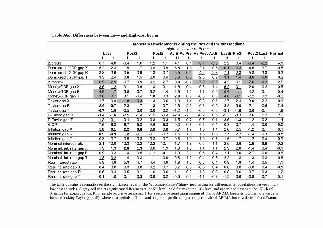
Table A6d: Differences between Low- and High-cost booms

The table contains information on the significance level of the Wilcoxon-Mann-Whitney test, testing for differences in populations between high-low-cost episodes. A grey cell depicts significant differences at the 5% level, bold figures at the 10% level and underlined figures at the 15% level.X stands for ex-post trends, R for simple recursive trends and T for a recursive trend using optimised Tramo ARIMA forecasts. Furthermore we derivforward-looking Taylor gaps (F), where next periods inflation and output are predicted by a one-period ahead ARIMA forecast derived from Tramo.

NormalH L H L H L H L H L H L H L

∆ credit 6.7 4.8 -0.4 1.6 1.2 1.1 4.1 0.1 -9.7 -3.8 2.2 0.4 -6.4 -2.2 4.1Dom. credit/GDP gap X 5.2 2.3 1.9 1.7 0.8 0.9 6.5 1.3 -2.1 0.5 10.1 3.3 -4.6 -3.7 -0.5Dom. credit/GDP gap R 3.8 3.6 0.5 0.9 1.3 -0.7 5.5 -0.5 -4.2 -2.3 7.1 2.3 -5.8 -3.3 -0.3Dom. credit/GDP gap T 3.3 2.4 0.8 1.5 2.0 0.4 3.6 0.0 -2.5 0.2 3.1 1.4 -3.6 -0.9 0.2∆ money 6.9 2.9 -0.7 0.9 -0.2 2.7 3.0 -0.1 -7.9 -2.8 4.2 -0.1 -7.6 -0.2 2.5Money/GDP gap X 3.6 1.2 0.1 -0.9 1.3 0.1 1.6 0.4 -0.6 -1.4 5.2 0.1 -2.0 -0.2 -0.5Money/GDP gap R 4.9 1.7 3.8 0.7 3.2 1.4 2.9 1.2 -1.1 0.6 5.4 1.1 -4.2 0.1 -0.4Money/GDP gap T 3.8 0.7 3.1 -0.4 1.8 0.3 2.8 0.3 -0.8 0.8 4.8 -0.1 -2.2 0.2 -0.2Taylor gap X -1.7 -0.9 -1.8 -0.3 -1.3 0.6 -1.3 -1.4 -0.8 0.5 -2.7 -2.4 3.0 2.2 -0.1Taylor gap R -2.4 -0.7 -2.3 -1.7 -1.3 -0.7 -2.8 -2.3 -0.8 -0.5 -3.2 -3.0 2.1 0.6 2.4Taylor gap T -0.7 1.0 -0.5 0.0 0.0 0.2 -1.2 -1.3 -0.8 -0.3 -3.1 -1.8 0.6 -0.1 1.9F-Taylor gap R -3.4 -1.6 -2.5 -1.4 -1.5 -0.4 -2.9 -2.1 -0.2 0.5 -5.3 -3.3 2.6 1.2 2.2F-Taylor gap T -1.3 0.1 -0.4 0.2 -0.3 0.3 -1.5 -0.7 -0.7 0.1 -2.6 -1.3 1.2 0.2 1.4∆ CPI 7.5 6.3 6.7 5.3 4.6 5.3 0.3 0.6 -0.5 0.4 0.8 0.7 -1.4 0.0 9.0Inflation gap X 1.8 0.1 2.2 0.8 0.8 0.8 0.7 1.7 1.5 1.4 2.0 2.5 -1.2 0.1 0.1Inflation gap R 0.9 -0.9 1.8 -0.7 -0.7 -0.2 1.6 1.9 1.3 0.8 2.7 2.2 -1.4 0.3 -0.8Inflation gap T 0.3 -0.7 0.9 -0.8 -0.8 -0.7 0.8 1.0 1.0 0.7 1.5 1.7 -1.2 0.4 -0.9Nominal interest rate 12.1 10.0 13.3 10.2 10.2 10.1 1.7 1.8 0.5 1.1 2.5 2.6 -1.5 0.5 10.2Nominal. int. rate gap X 1.9 1.3 2.8 1.3 0.6 1.9 1.9 1.8 1.4 1.1 2.9 2.8 -1.4 0.4 -0.1Nominal. int. rate gap R 0.9 0.3 1.4 0.5 -1.7 -0.1 1.0 2.1 0.5 0.4 2.1 3.0 -2.7 -0.6 -0.6Nominal. int. rate gap T 1.3 0.2 1.4 0.3 -1.1 0.0 0.8 1.2 0.4 0.3 2.2 1.8 -1.3 -0.3 -0.6Real interest rate 5.8 4.8 5.3 4.7 4.4 4.9 1.8 1.2 -0.5 0.4 0.8 1.8 -1.4 0.5 1.1Real int. rate gap X 0.4 0.8 0.3 0.8 0.2 0.7 0.7 0.6 -0.5 0.4 0.8 0.8 -0.8 0.4 -0.1Real int. rate gap R -0.6 0.4 -0.5 0.1 -1.6 -0.6 -1.1 0.0 -1.3 -0.3 -0.8 -0.6 -0.7 -0.3 1.2Real int. rate gap T -0.1 1.0 0.1 0.3 -0.9 0.2 -0.3 0.3 -1.1 -0.2 -1.3 0.6 -0.9 -0.7 0.1

Monetary Developments during the 70's and the 80's MediansHigh- vs. Low-cost Booms

Last Post1 Post2-Last Post2 Av.B-Av.Pre Av.Post-Av.B LastB-Pre2

Figure A

Australia

Belgium

C

Canada

1. Canada

4.4

4.5

4.6

4.7

4.8

4.9

5.0

5.1

5.2

1970 1975 1980 1985 1990 1995 2000

Aggregate Trend

HL

4.2

4.4

4.6

4.8

5.0

5.2

5.4

1970 1975 1980 1985 1990 1995 2000

Aggregate Equity Real estate

4.0

4.4

4.8

5.2

5.6

6.0

1970 1975 1980 1985 1990 1995 20004.5

4.6

4.7

4.8

4.9

5.0

5.1

5.2

5.3

1970 1975 1980 1985 1990 1995 2000

L

4.5

4.6

4.7

4.8

4.9

5.0

1970 1975 1980 1985 1990 1995 2000

H

4.2

4.4

4.6

4.8

5.0

5.2

5.4

5.6

1970 1975 1980 1985 1990 1995 2000

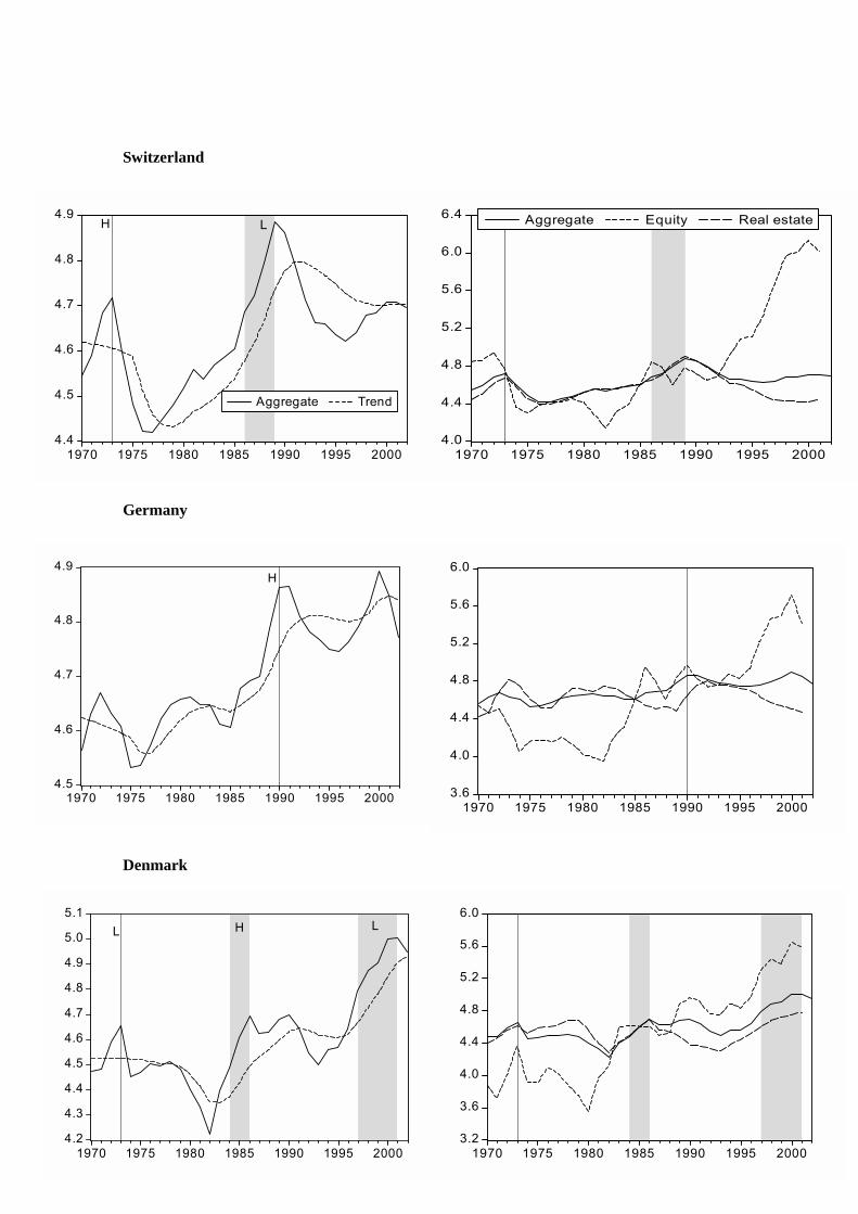
48

Switzerland

Germany

Denmark

4.4

4.5

4.6

4.7

4.8

4.9

1970 1975 1980 1985 1990 1995 2000

Aggregate Trend

H L

4.0

4.4

4.8

5.2

5.6

6.0

6.4

1970 1975 1980 1985 1990 1995 2000

Aggregate Equity Real estate

4.5

4.6

4.7

4.8

4.9

1970 1975 1980 1985 1990 1995 2000

H

3.6

4.0

4.4

4.8

5.2

5.6

6.0

1970 1975 1980 1985 1990 1995 2000

4.2

4.3

4.4

4.5

4.6

4.7

4.8

4.9

5.0

5.1

1970 1975 1980 1985 1990 1995 2000

HL L

3.2

3.6

4.0

4.4

4.8

5.2

5.6

6.0

1970 1975 1980 1985 1990 1995 2000

49

Spain

Finland

France

4.4

4.6

4.8

5.0

5.2

5.4

5.6

1970 1975 1980 1985 1990 1995 2000

Aggregate Trend H L

4.0

4.5

5.0

5.5

6.0

6.5

7.0

1970 1975 1980 1985 1990 1995 2000

Aggregate Equity Real estate

4.0

4.2

4.4

4.6

4.8

5.0

5.2

5.4

5.6

1970 1975 1980 1985 1990 1995 2000

H H

3.5

4.0

4.5

5.0

5.5

6.0

6.5

7.0

7.5

1970 1975 1980 1985 1990 1995 2000

4.5

4.6

4.7

4.8

4.9

5.0

5.1

1970 1975 1980 1985 1990 1995 2000

LL

4.0

4.4

4.8

5.2

5.6

6.0

6.4

1970 1975 1980 1985 1990 1995 2000

50

Ireland

Italy

Japan

4.0

4.4

4.8

5.2

5.6

6.0

6.4

6.8

1970 1975 1980 1985 1990 1995 2000

Aggregate Equity Real estate

4.4

4.6

4.8

5.0

5.2

5.4

5.6

5.8

6.0

1970 1975 1980 1985 1990 1995 2000

Aggregate Trend

L L L

4.4

4.5

4.6

4.7

4.8

4.9

5.0

5.1

1970 1975 1980 1985 1990 1995 2000

L L

3.6

4.0

4.4

4.8

5.2

5.6

6.0

1970 1975 1980 1985 1990 1995 2000

3.6

4.0

4.4

4.8

5.2

5.6

1970 1975 1980 1985 1990 1995 20004.2

4.3

4.4

4.5

4.6

4.7

4.8

4.9

5.0

5.1

1970 1975 1980 1985 1990 1995 2000

HH

51

Netherlands

2.

3.

4.

5.

6.

New Zealand

7.

8.

9.

10.

11.

Norway

12.

13.

14.

15.

16. 3.8

4.0

4.2

4.4

4.6

4.8

5.0

5.2

5.4

1970 1975 1980 1985 1990 1995 2000

3.8

4.0

4.2

4.4

4.6

4.8

5.0

5.2

1970 1975 1980 1985 1990 1995 2000

4.4

4.6

4.8

5.0

5.2

5.4

5.6

1970 1975 1980 1985 1990 1995 2000

Aggregate Trend

L L L

3.5

4.0

4.5

5.0

5.5

6.0

6.5

1970 1975 1980 1985 1990 1995 2000

Aggregate Equity Real estate

4.3

4.4

4.5

4.6

4.7

4.8

4.9

5.0

1970 1975 1980 1985 1990 1995 2000

L L

4.0

4.2

4.4

4.6

4.8

5.0

5.2

1970 1975 1980 1985 1990 1995 2000

HL L

52

Sweden

United Kingdom

United States

4.0

4.4

4.8

5.2

5.6

6.0

6.4

1970 1975 1980 1985 1990 1995 2000

4.0

4.4

4.8

5.2

5.6

6.0

1970 1975 1980 1985 1990 1995 2000

3.6

4.0

4.4

4.8

5.2

5.6

6.0

6.4

6.8

1970 1975 1980 1985 1990 1995 2000

Aggregate Equity Real estate

4.4

4.6

4.8

5.0

5.2

5.4

5.6

5.8

1970 1975 1980 1985 1990 1995 2000

Aggregate Trend

H L

4.2

4.4

4.6

4.8

5.0

5.2

5.4

1970 1975 1980 1985 1990 1995 2000

H H L

4.4

4.6

4.8

5.0

5.2

5.4

1970 1975 1980 1985 1990 1995 2000

L L

53

The Data

The data frequency is annual. The period covered is 1970 until 2002 for most series and most

countries. We consider 18 countries, which are Australia, Belgium, Canada, Switzerland, Germany,

Denmark, Spain, Finland, France, Ireland, Italy, Japan, Netherlands, Norway, New Zealand, Sweden,

US and UK. The asset price indices have been kindly supplied by Steve Arthur and Claudio Borio

from the BIS (See Borio, Kennedy and Prowse (1994) and Borio and Lowe (2001) on these indices).

The aggregate indices are weighted by the actual share of the asset components (equity, residential

property, commercial property) in the respective economy. We used the real asset price indices as

deflated by consumer prices by the BIS.

The following data are from the OECD Economic Outlook, with the series code in parenthesis:

Real private consumption (CPV), consumer prices (CPI), the nominal effective exchange rate

(EXCHEB), real housing investment (IHR), real private investment (IPV), a broad monetary aggregate

(MONEYS), the short term interest rate (IRS), nominal and real GDP (GDP and GDPV). We

corrected the German growth rates for GDP, investment, housing investment and consumption for the

unification effect in 1991, using the West German growth rate for 1991.

Domestic credit is from the IMF’s International Financial Statistics, code 32. For the euro area

countries domestic credit has been updated from 1999 until 2002 with growth rates obtained from the

ECB’s Monetary Transmission Network database. The credit series showed huge structural breaks.

Whenever the IFS codes signalled a structural break and simultaneously the TRAMO software

indicated a structural break (level shift) based on the time series characteristics, we let TRAMO

estimate the size of the structural break and used the (backward) corrected data. Credit data for

Belgium, France and the Netherlands are interpolated for the year 1998.

Monetary aggregates for the Euro Area countries are M3 data from the ECB’s Monetary Transmission

Network database.

For France, UK, Ireland, Italy and Denmark interest rates are form the AMECO database. In order to

use longer time series to improve the trend estimates for the early periods we used the IFS money

market rate, line 60b, assuming parallel shifts in the yield curve for the following countries:

Switzerland 1969-1973, Spain 1974-1976, Norway 1972-1978 and Sweden 1966-1981.

The rate of change of the real effective exchange rate is computed by simply adding the growth rates

of nominal effective exchange rate index and domestic inflation. It thus neglects price developments

of trading partners.

The real interest rate is simply the difference between the short term interest rate and current inflation.

The ratios to GDP for output components were computed by dividing the real variable by real GDP.

The ratios for the nominal variables, money and credit were computed as ratios to nominal GDP. The

54

recursive trends were derived by extending the window for the HP filter period by period. The starting

window for the first (non-recursive) trend estimates were the following, 1970-1975 for the real

aggregate asset price indices, interest rates as well as the monetary aggregate and from as early as data

were available (usually 1963) until 1970 for all other variables. The base periods differ slightly due to

missing data availability for some countries with regard to the respective variable: the base period for

interest rates for Spain and New Zealand is 1974-1979 and for Norway 1972-1977. The TRAMO

software needs a minimum of 12 observations to identify an ARIMA model. Thus the base window to

calculate the HP trend was extended accordingly.

There were three cases where we artificially overturned the automatic boom identification. For New

Zealand in 1985 the real aggregate asset price gap fell below 10% due to a massive hike in inflation

while nominal asset prices continued to rise. We chose to prolong rather than interrupt the boom so

that the whole period 84-87 can be considered as one instead of two (84 and 86-87) booms. Similar

argumentation applied to Ireland 1988 and Norway 1999. In both years real asset prices were still

rising although falling below the threshold due to the increase in the trend. In order to maintain a

continuous boom period we classified these two years also as boom years.

The equity price gap for Spain between 1983-1986 is the percent difference using the average of the

trend and the series as opposed to log differences as the trend turned out to be negative in this period.

The five different measures of the Taylor gaps (two of which forecast based) are defined as follows,

where i is the nominal interest rate, r the real interest rate, π the inflation rate, y real GDP and

variables with a star denote trend values:

Taylor gap X: it – [rt* + πt + 0.5(πt - πt*) + 0.5(yt – yt*)], where r*, π* and y* are the ex-post HP

trends derived with λ=100.

Taylor gap R: it – [rt* + πt + 0.5(πt - πt*) + 0.5(yt – yt*)], where r*, π* and y* are the recursive HP

trends derived with λ=1000.

Taylor gap T: it – [rt* + πt + 0.5(πt - πt*) + 0.5(yt – yt*)], where r*, π* and y* are the recursive HP

trends derived with λ=1000 where at each point in time the optimal ARIMA model for each of the

three variables is identified (by TRAMO) in order to produce a three period forecast. The recursive

HP trend for each period in time is then derived using the series including three forecast values,

extending the current sample edge.

F-Taylor gap R: it – [rt* + πt + 0.5(tπt+1 - tπt+1*) + 0.5(tyt+1 – tyt+1*)], where r* is the recursive HP

trend derived with λ=1000. tπt+1 and tyt+1 are the one period ahead forecasts derived by an optimised

ARIMA model, which is newly identified for each country at each point in time (by TRAMO). tπt+1*

and tyt+1* are one period ahead forecasts of the HP trend using again an optimised ARIMA model.

55

F-Taylor gap T: This is the same as F-Taylor gap R, except that three period optimised ARIMA model

forecasts are used to derive the HP trends π* and y* before the one period forecasts of tπt+1* and tyt+1*

are computed.

The Wilcoxon-Mann-Whitney Test

The Wilcoxon-Mann-Whitney test is a non-parametric test for differences in populations. The

assumptions are simply that each sample is a random sample from the population it represents, that the

two samples are independent from each other and that the measurement scale is at least ordinal.

To derive the test statistic one first combines the two series and then orders all observations by size.

Then one computes the sum of the ranks (in the combined series) for the two samples. The null

hypothesis that there is no difference between the two populations will be rejected when the sum of

the ranks of the two samples is relatively different. If the number of observations in at least one of the

two samples exceeds 10 (see e.g. Newbold et al., 2003), which is always true in our case, the test

statistic quickly approaches a normal distribution. The test statistic used for a two-sided test is

12/)1(2/)1(5.0

++−±

=Nmn

NmWz x , where Wx is the sum of the ranks of the smaller sample, m and n are

the number of observations in the smaller and larger sample, respectively and N=m+n.

Under the additional assumption that the only difference between the two populations is the mean, the

Wilcoxon-Mann-Whitney test can be interpreted as a test for equality of means. Even in this case it is

more powerful than a standard two sample t-test for small samples as it does not require the normality

assumption. The tests have been applied to all periods except the third, fourth and fifth boom years.

Table A7 shows that the sample for high- and low-cost booms gets too small to draw reasonable

conclusions.

Table A7

Sample size for different periods: overall, high and low cost booms

B1, Last, all others B2 B3 B4 B5 Norm

Overall 38 31 20 17 10 about 240

High cost 14 11 9 8 5 -

Low cost 24 20 11 9 5 -