asset allocation, time diversification and portfolio ...asset allocation, time diversification and...

Technology and Investment, 2011, 2, 92-104 doi:10.4236/ti.2011.22010 Published Online May 2011 (http://www.SciRP.org/journal/ti)

Copyright © 2011 SciRes. TI

Asset Allocation, Time Diversification and Portfolio Optimization for Retirement

Kamphol Panyagometh NIDA Business School, Bangkok, Thailand

E-mail: [email protected], [email protected] Received February 17, 2011; revised April 6, 2011; accepted April 10, 2011

Abstract Using the data of stock, commodity and bond indexes from 2002 to November 2010, this research was car-ried out by employing Bootstrapping Simulation technique to find an optimal portfolio (portfolio optimiza-tion) for retirement, and the effect of diversification based on increased length of investment period (time diversification) with respect to the lengths of retirement investment period and the amounts required for spending after retirement in various occasions. The study analyzed for an optimal allocation of common stock, commodity and government bond to achieve the target rate of return for retirement by minimizing the portfolio risk as measured from the standard deviation. Apart from the standard deviation of the rate of return of the investment portfolio, this study also viewed the risk based on the Value at Risk concept to study the downside risk of the investment portfolio for retirement. Keywords: Asset Allocation, Time Diversification, Portfolio Optimization, Bootstrapping Simulation

1. Introduction Nowadays the structure of Thai society is one with a growing proportion of the elderly. While medical tech-nology has experienced a rapid pace of advancement, the average age of the population is increasing; which means that Thai people need to be planning to save money for longer retirement life. Data available at the National Sta-tistical Office (NSO) showed that 73 percent of the over-all population was not a member of any retirement fund; where only 23.3 percent was. Therefore, the government devised a policy to push for saving fund establishment in the form of retirement saving fund on the grounds that, in the long run, the elderly with neither money nor security shall become a burden to family members while gov-ernmental welfare might not be thoroughly accessible. For this reason, the Thai society should place importance on the systematic, conventional, and consistent long term investment and saving system especially during its working years, where it should start to save and invest through funds or investment and saving systems under expert supervision in order to be able to manage its in-vestment for generating income stream during retirement efficiently.

This research was carried out to find an optimal in-vestment ratio between common stock, commodity and

bond in investment portfolio (portfolio optimization) for retirement, and the effect of diversification based on in-creased length of investment period (time diversification). The study employed Bootstrapping Simulation technique to generate long term rates of return with respect to the lengths of retirement investment period and the amounts required for spending after retirement in various occa-sions; and analyzed for an optimal investment ratio be-tween common stock and government bond to achieve the target rate of return for retirement by minimizing the portfolio risk as measured from the standard deviation. Apart from the standard deviation of the rate of return of the investment portfolio, this study also viewed the risk based on the Value at Risk concept to study the down-side risk of the investment portfolio for retirement.

The rest of the paper is organized as follows. Section 2 reviews related literature. Section 3 discusses the re-search data used. Section 4 explains research methodol-ogy and Bootstrapping simulation technique. Section 5 discusses the results of the study, and Section 6 con-cludes. 2. Literature Review

Levy [1] illustrated the time diversification phenomenon by studying the past performance of common stocks and

K. PANYAGOMETH 93 government bonds at different lengths of investment pe-riod, and found that common stocks offered better rate of return than government bonds did in all investments with 25 years period. This outcome held true during the in-vestment years 1926-1977. Reichenstein [2] employed the same techniques and research methodologies as Levy [1] did and proved that the risk of investment portfolio was dependent on the investment period. Leibowitz and Langetieg [3] developed a model under the hypothesis that common stocks had a risk premium of 4% higher than that of debentures. This risk premium value was less than the actual value obtained from the data since 1926, where common stocks had a risk premium of 7% higher than that of debentures. This study showed that while the risk premium became less, the benefits of common stocks as compared with debentures became lower for both short-term and long-term investments. Butler and Domian [4] studied a long-term rate of return of retire-ment portfolios of common stocks and debentures by attempting various asset allocation strategies. The out-come revealed that as the length of pre-retirement in-vestment period was increased, common stock invest-ment risk was greatly reduced as compared with that of debentures; and when the pre-retirement investment pe-riod reached or exceeded 30 years, the chance that com-mon stocks would yield less than debentures would be less than 4%. Bjorn and Persson [5] suggested that long-term investors should invest in a high proportion of risky assets. The study showed that efficient portfolios with long investment period would have a higher propor-tion of share investment as compared with efficient portfolios with only 1 year investment period. Strong and Taylor [6] examined the relationship between security returns and investment periods, and pointed out the time diversification phenomenon of optimal investment port-folio. Hickman, Hunter, Byrd, Beck, and Terpening [7] employed Bootstrapping technique in the monthly rate of return study during 1926-1997 and found that the chance for monthly investment in common stocks to yield less than government bonds dropped from 39% to 6% when the pre-retirement investment period increased from 1 year to 30 years. Gollier [8] proposed a theory of time diversification and absolute risk aversion for wealth. The research found that time diversification phenomenon would occur in the case where investors discriminated between wealth-related risk and consumption-related risk. Howe and Mistic [9] studied the impact of personal in-come tax on the return of various asset classes on the retirement date. Guo and Darnell [10] tried to prove the existence of time diversification by using past returns data of S&P500, T-bill, and T-Bond indices during 1802-2002. This study found that the benefits of time diversification depended on the risk of security index

return rate when compared with the risk of government bond return rate. Mukherji [11] published the study out-come which contributed to time diversification research efforts through the use of Block Bootstrap method to model long-term rate of returns and analyze the invest-ment diversification of 6 categories of financial assets to find an optimal investment portfolio by minimizing the downside risk based on a number of required rates of return. Alles [12] studied the effect of downside protec-tion development cost and time diversification among Stock Exchange investors in Bangladesh, Sri Lanka, In-dia, and Pakistan using Bootstrapping methodology where the investment period ranged from 1 to 20 years. It was found that the cost of downside protection varied from country to country, and was lessened with the in-crease in the length of investment period. This is consis-tent with the benefit of time diversification. Pan-yagometh [13] demonstrated the benefit of time diversi-fication by showing that an investor’s starting the retire-ment investment early in order to have a longer pre-re-tirement investment period not only reduced the monthly pre-retirement investment amount, but also mitigated the probability of ruin associated with the retirement invest-ment.

3. Research Data This study employed the 2002-November 2010 data comprising the Stock Exchange of Thailand total return index (SET TRI) calculated by the Stock Exchange of Thailand, representing investment in common stock asset class; the Rogers International Commodity Index (RICI®) calculated by Beeland Interests, Inc., representing in-vestment in commodity asset class; and the government bond total return index (TBMA total return index, BOND TRI) calculated by the Thai Bond Market Association, representing investment in government bond asset class.

SET TRI is an index calculated from all types of return on security investment so as to have all of them reflected; namely, returns based on capital gain/loss; rights to sub-scribe for shares, which is granted for existing sharehold-ers to buy new shares usually at the price lower than their market price at that moment; and dividends, which are the share of profits paid to shareholders, with supplemental assumption that the dividends received shall again be invested in securities (reinvest).

RICI® is a composite, USD based, total return index calculated from 37 commodities from 13 international exchanges. It represents the value of a basket of com-modities consumed in the global economy, ranging from agricultural to energy and metals products. The index is divided into three sub-indices, which reflect the three sub-segments of the RICI - RICI Agriculture, RICI En-


K. PANYAGOMETH


94

ergy and RICI Metals. The sub-indices’ contribution to main index from the beginning are Agriculture - 34.90%, Energy - 44.00%, Metals - 21.10% according to the RICI Handbook.

BOND TRI is an index obtained through the same cal-culation methodology as the index of European of Finan-cial Analysts Societies, or EFFAS; which is based on international principle. The calculation makes use of all government bonds which are registered bonds listed at the Thai Bond Dealing Centre; not including state owned enterprise bonds, Bank of Thailand bonds, Financial In-stitution Development Fund bonds, etc. in order for the index to exclusively reflect the market situation of gov-ernment bonds, which are deemed truly risk-free with regard to default in payment of interest and principal. The weighted average executed yield is used in the cal-culation, where each item of the executed yield is weighted by its value traded. After the weighted average executed yield is obtained, the clean price of each bond is then calculated. The resulting index shall therefore represent the movements of government bond market on a daily basis, where BOND TRI includes the interest due on the index calculation date within its calculation.

Table 1 presents SET TRI, RICI® and BOND TRI monthly data during 2002 - November 2010. Table 2 shows statistics information of the research data present-ing the average monthly (annual) return on investment in SET TRI, RICI® and BOND TRI of 1.57% (18.84%), 0.75% (9.00%) and 0.41% (4.92%) respectively; where the standard deviation of the monthly (annual) return on investment in SET TRI, RICI® and BOND TRI reads 6.76% (23.42%), 5.46% (18.91%) and 1.90% (6.58%). As foreseen, common stock is an asset which provides a higher return than bond, but it has a higher risk as well. With regard to the value −0.1160 of the correlation coef-ficient between common stock and bond, the value −0.2820 of the correlation coefficient between bond and commodity, and the value 0.3771 of the correlation coef-ficient between stock and commodity, investors who invest in common stock, commodity and bond in their investment portfolio shall be able to benefit from diver-sification since these asset classes have low or even negative correlation coefficients. 4. Research Methodology: Bootstrapping

Simulation Bootstrapping Simulation technique involves randomly and repeatedly sampling values of data in order to esti-mate the distributions of required statistics. Bootstrap-ping Simulation can reduce the risk of assessment error occurrence when the true parameters of the rate of return distribution are unknown. Singh [14] showed that the

distribution of data estimated by Non-parametric Boot-strap method has high degree of accuracy.

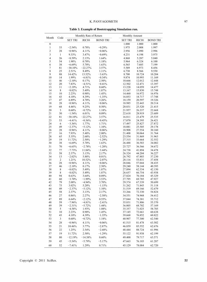
Steps to Performing Bootstrapping Simulation: Suppose we want to run Bootstrapping Simulation to

model a return on monthly investment of 1 Baht per month in SET TRI, RICI®, and BOND TRI for a period of 5 years or 60 months:

Step 1: Assign codes to the monthly rate of return data of SET TRI, RICI® and BOND TRI during 2002 - No-vember 2010 as shown in Table 1.

Step 2: Simulate the monthly return of SET TRI, RICI® and BOND TRI in each month for 60 months. The monthly return of each month is obtained through generating a random number between 1 and 106, and using the return rate of SET TRI, RICI® and BOND TRI in the month which matches the number generated as monthly return for that month. An example of a simu-lation run is shown in Table 3 in which a random number generated for month 1 is 33, which corre-sponds to a monthly rate of return of 29/10/2004, the value of which was −2.54%, 0.78% and −0.29% for SET TRI, RICI® and BOND TRI respectively; while a random number generated for month 20 is 3, which corresponds to a monthly rate of return of 30/4/2002, the value of which was 0.60%, −0.72% and 1.18% for SET TRI, RICI® and BOND TRI respectively. Through this method, the monthly rate of return of 60 months can be obtained, as shown in Table 3.

Step 3: Calculate the return amount from the investment in SET TRI, RICI® and BOND TRI for each month as shown in Table 3, starting from investing 1 Baht in month 0 (beginning of month 1). In month 1, SET TRI offers −2.54% rate of return, and RICI® offers 0.78%, while BOND TRI offers −0.29%; thus after a month has passed the money invested in SET TRI is equal to 1 × (1 − 0.0254) = 0.9746, and the money invested in RICI® is equal to 1 × (1 + 0.0075) = 1.0075 while the money in-vested in BOND TRI is equal to 1 × (1 − 0.0029) = 0.9971. Then add 1 Baht monthly amount being invested each month yielding the result at the end of month 1 (be-ginning of month 2) of 1.9746, 2.0075 and 1.9971 for SET TRI, RICI® and BOND TRI respectively. In month 2, SET TRI rate of return is −0.96%, and that of RICI® is 4.11% while that of BOND TRI is −0.06%; therefore, after another month has passed the investment in SET TRI is equal to 1.9746 × (1 − 0.0096) = 1.9556, and the in-vestment in RICI® is equal to 2.0075 × (1 + 0.0411) = 2.0900 the while the investment in BOND TRI is equal to 1.9971 × (1 − 0.0006) = 1.9959. Again add 1 Baht monthly amount being invested each month yielding the result at the end of month 2 (beginning of month 3) of 2.9556, 3.0900 and 2.9959 for SET TRI, RICI® and BOND TRI respectively. The calculation proceeds ac-

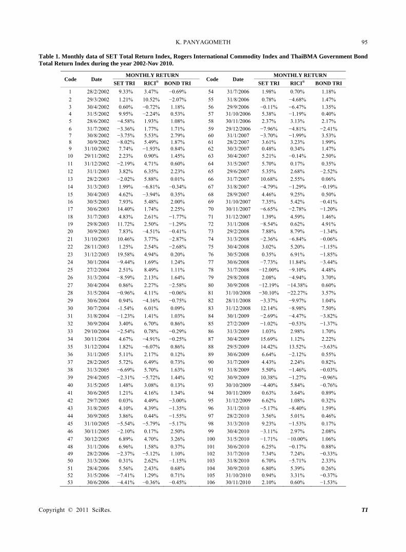
K. PANYAGOMETH 95 Table 1. Monthly data of SET Total Return Index, Rogers International Commodity Index and ThaiBMA Government Bond Total Return Index during the year 2002-Nov 2010.

MONTHLY RETURN MONTHLY RETURN Code Date

SET TRI RICI® BOND TRICode Date

SET TRI RICI® BOND TRI

1 28/2/2002 9.33% 3.47% −0.69% 54 31/7/2006 1.98% 0.70% 1.18%

2 29/3/2002 1.21% 10.52% −2.07% 55 31/8/2006 0.78% −4.68% 1.47% 3 30/4/2002 0.60% −0.72% 1.18% 56 29/9/2006 −0.11% −6.47% 1.35% 4 31/5/2002 9.95% −2.24% 0.53% 57 31/10/2006 5.38% −1.19% 0.40% 5 28/6/2002 −4.58% 1.93% 1.08% 58 30/11/2006 2.37% 3.13% 2.17%

6 31/7/2002 −3.36% 1.77% 1.71% 59 29/12/2006 −7.96% −4.81% −2.41% 7 30/8/2002 −3.75% 5.53% 2.79% 60 31/1/2007 −3.70% −1.99% 3.53% 8 30/9/2002 −8.02% 5.49% 1.87% 61 28/2/2007 3.61% 3.23% 1.99% 9 31/10/2002 7.74% −1.93% 0.84% 62 30/3/2007 0.48% 0.34% 1.47% 10 29/11/2002 2.23% 0.90% 1.45% 63 30/4/2007 5.21% −0.14% 2.50%

11 31/12/2002 −2.19% 4.71% 0.60% 64 31/5/2007 5.70% 0.17% 0.35%

12 31/1/2003 3.82% 6.35% 2.23% 65 29/6/2007 5.35% 2.68% −2.52%

13 28/2/2003 −2.02% 5.88% 0.01% 66 31/7/2007 10.68% 2.55% 0.06%

14 31/3/2003 1.99% −6.81% −0.34% 67 31/8/2007 −4.79% −1.29% −0.19%

15 30/4/2003 4.62% −3.94% 0.35% 68 28/9/2007 4.46% 9.25% 0.50% 16 30/5/2003 7.93% 5.48% 2.00% 69 31/10/2007 7.35% 5.42% −0.41% 17 30/6/2003 14.40% 1.74% 2.25% 70 30/11/2007 −6.65% −2.78% −1.20%

18 31/7/2003 4.83% 2.61% −1.77% 71 31/12/2007 1.39% 4.59% 1.46% 19 29/8/2003 11.72% 2.50% −1.29% 72 31/1/2008 −8.54% 0.62% 4.91% 20 30/9/2003 7.83% −4.51% −0.41% 73 29/2/2008 7.88% 8.79% −1.34%

21 31/10/2003 10.46% 3.77% −2.87% 74 31/3/2008 −2.36% −6.84% −0.06%

22 28/11/2003 1.25% 2.54% −2.68% 75 30/4/2008 3.02% 5.20% −1.15%

23 31/12/2003 19.58% 4.94% 0.20% 76 30/5/2008 0.35% 6.91% −1.85%

24 30/1/2004 −9.44% 1.69% 1.24% 77 30/6/2008 −7.73% 11.84% −3.44%

25 27/2/2004 2.51% 8.49% 1.11% 78 31/7/2008 −12.00% −9.10% 4.48%

26 31/3/2004 −8.59% 2.13% 1.64% 79 29/8/2008 2.08% −4.94% 3.70%

27 30/4/2004 0.86% 2.27% −2.58% 80 30/9/2008 −12.19% −14.38% 0.60%

28 31/5/2004 −0.96% 4.11% −0.06% 81 31/10/2008 −30.10% −22.27% 3.57%

29 30/6/2004 0.94% −4.16% −0.75% 82 28/11/2008 −3.37% −9.97% 1.04%

30 30/7/2004 -1.54% 6.01% 0.09% 83 31/12/2008 12.14% −8.98% 7.50%

31 31/8/2004 −1.23% 1.41% 1.03% 84 30/1/2009 −2.69% −4.47% −3.82%

32 30/9/2004 3.40% 6.70% 0.86% 85 27/2/2009 −1.02% −0.53% −1.37%

33 29/10/2004 −2.54% 0.78% −0.29% 86 31/3/2009 1.03% 2.98% 1.70%

34 30/11/2004 4.67% −4.91% −0.25% 87 30/4/2009 15.69% 1.12% 2.22%

35 31/12/2004 1.82% −6.07% 0.86% 88 29/5/2009 14.42% 13.52% −3.63%

36 31/1/2005 5.11% 2.17% 0.12% 89 30/6/2009 6.64% −2.12% 0.55%

37 28/2/2005 5.72% 6.49% 0.73% 90 31/7/2009 4.43% 2.24% 0.82%

38 31/3/2005 −6.69% 5.70% 1.63% 91 31/8/2009 5.50% −1.46% −0.03%

39 29/4/2005 −2.31% −5.72% 1.44% 92 30/9/2009 10.38% −1.27% −0.96%

40 31/5/2005 1.48% 3.08% 0.13% 93 30/10/2009 −4.40% 5.84% −0.76%

41 30/6/2005 1.21% 4.16% 1.34% 94 30/11/2009 0.63% 3.64% 0.89%

42 29/7/2005 0.03% 4.49% −3.00% 95 31/12/2009 6.62% 1.08% 0.32%

43 31/8/2005 4.10% 4.39% −1.35% 96 31/1/2010 −5.17% −8.40% 1.59%

44 30/9/2005 3.86% 0.44% −1.55% 97 28/2/2010 3.56% 5.01% 0.46%

45 31/10/2005 −5.54% −5.79% −5.17% 98 31/3/2010 9.23% −1.53% 0.17%

46 30/11/2005 −2.10% 0.17% 2.50% 99 30/4/2010 −3.11% 2.97% 2.08%

47 30/12/2005 6.89% 4.70% 3.26% 100 31/5/2010 −1.71% −10.00% 1.06%

48 31/1/2006 6.96% 1.58% 0.37% 101 30/6/2010 6.25% −0.17% 0.88% 49 28/2/2006 −2.37% −5.12% 1.10% 102 31/7/2010 7.34% 7.24% −0.33% 50 31/3/2006 0.31% 2.62% −1.15% 103 31/8/2010 6.70% −5.71% 2.33%

51 28/4/2006 5.56% 2.43% 0.68% 104 30/9/2010 6.80% 5.39% 0.26% 52 31/5/2006 −7.41% 1.29% 0.71% 105 31/10/2010 0.94% 3.31% −0.37% 53 30/6/2006 −4.41% −0.36% −0.45% 106 30/11/2010 2.10% 0.60% −1.53%


K. PANYAGOMETH96 Table 2. Statistics of SET Total Return Index, Rogers In-ternational Commodity Index and ThaiBMA Government Bond Total Return Index during the year 2002-Nov 2010.

MONTHLY RETURN


Mean 1.57% 0.75% 0.41%

Standard Deviation 6.76% 5.46% 1.90%

Max 19.58% 13.52% 7.50%

Min −30.10% −22.27% −5.17%

CORRELATION MATRIX


SET TRI 1.0000

RICI® 0.3771 1.0000

BOND TRI −0.1160 −0.2820 1.0000

cordingly until the amount of investment in SET TRI, RICI® and BOND TRI at the end of the month 60, which is equal to 45.129, 78.084 and 62.720 is ob-tained as shown in Table 3. For the reason that in ran-domization, the rate of return of SET TRI, RICI® and BOND TRI in the same month has been used, the outcome of Bootstrapping Simulation run therefore has already taken into account the rela-tionship among SET TRI, RICI® and BOND TRI rate of return, which is readily reflected in the correlation coefficients of this simulation run.

Step 4: Calculate the investment rate of return using the “Rate” function of Excel to determine the monthly rate of return. Given NPER = 60 (60 month invest-ment), PMT = −3 (investment of 3 Baht each month, comprising 1 Baht investment in SET TRI, another 1 Baht investment in RICI® and another 1 Baht in BOND TRI), PV = 0, FV = 185.933 (the total amount of investment in SET TRI, RICI® and BOND TRI at the end of month 60), and TYPE = 1 (as investment starts at the beginning of each month); the resulting return on investment of 0.106% per month or 1.272% per year is obtained.

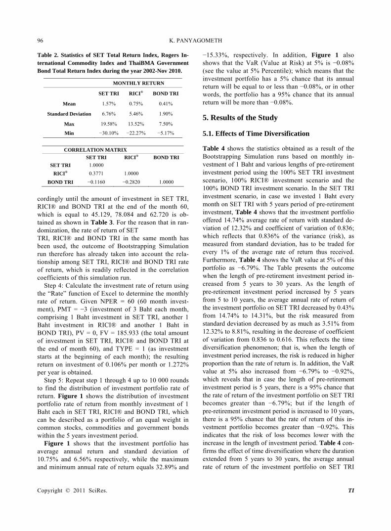
Step 5: Repeat step 1 through 4 up to 10 000 rounds to find the distribution of investment portfolio rate of return. Figure 1 shows the distribution of investment portfolio rate of return from monthly investment of 1 Baht each in SET TRI, RICI® and BOND TRI, which can be described as a portfolio of an equal weight in common stocks, commodities and government bonds within the 5 years investment period.

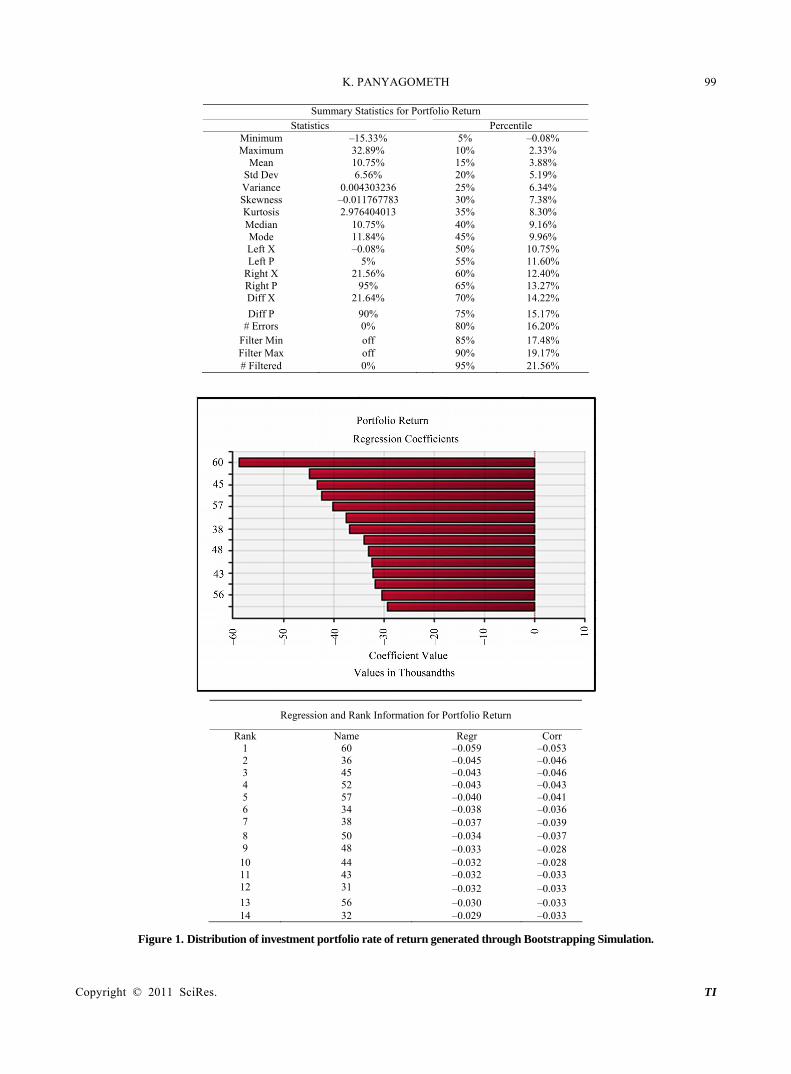
Figure 1 shows that the investment portfolio has average annual return and standard deviation of 10.75% and 6.56% respectively, while the maximum and minimum annual rate of return equals 32.89% and

−15.33%, respectively. In addition, Figure 1 also shows that the VaR (Value at Risk) at 5% is −0.08% (see the value at 5% Percentile); which means that the investment portfolio has a 5% chance that its annual return will be equal to or less than −0.08%, or in other words, the portfolio has a 95% chance that its annual return will be more than −0.08%.

5. Results of the Study 5.1. Effects of Time Diversification

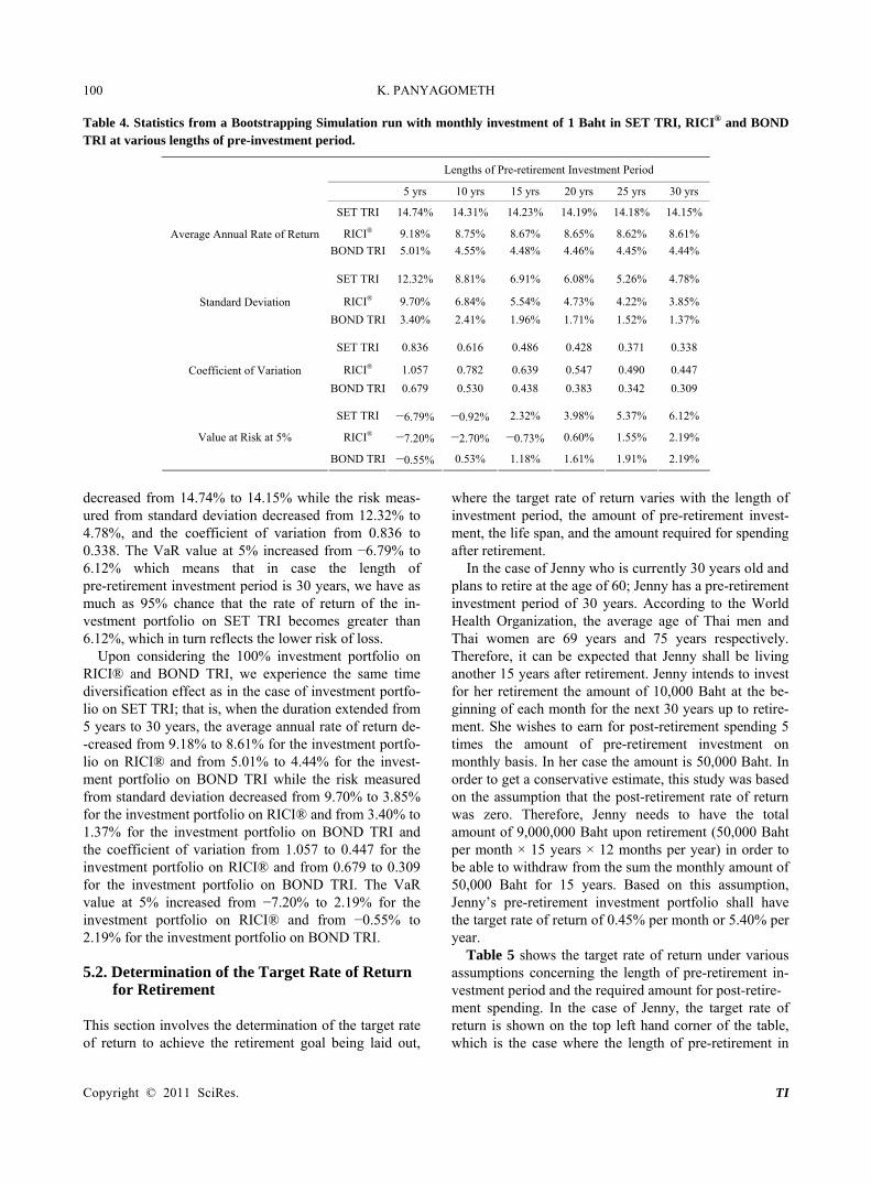
Table 4 shows the statistics obtained as a result of the Bootstrapping Simulation runs based on monthly in-vestment of 1 Baht and various lengths of pre-retirement investment period using the 100% SET TRI investment scenario, 100% RICI® investment scenario and the 100% BOND TRI investment scenario. In the SET TRI investment scenario, in case we invested 1 Baht every month on SET TRI with 5 years period of pre-retirement investment, Table 4 shows that the investment portfolio offered 14.74% average rate of return with standard de-viation of 12.32% and coefficient of variation of 0.836; which reflects that 0.836% of the variance (risk), as measured from standard deviation, has to be traded for every 1% of the average rate of return thus received. Furthermore, Table 4 shows the VaR value at 5% of this portfolio as −6.79%. The Table presents the outcome when the length of pre-retirement investment period in-creased from 5 years to 30 years. As the length of pre-retirement investment period increased by 5 years from 5 to 10 years, the average annual rate of return of the investment portfolio on SET TRI decreased by 0.43% from 14.74% to 14.31%, but the risk measured from standard deviation decreased by as much as 3.51% from 12.32% to 8.81%, resulting in the decrease of coefficient of variation from 0.836 to 0.616. This reflects the time diversification phenomenon; that is, when the length of investment period increases, the risk is reduced in higher proportion than the rate of return is. In addition, the VaR value at 5% also increased from −6.79% to −0.92%, which reveals that in case the length of pre-retirement investment period is 5 years, there is a 95% chance that the rate of return of the investment portfolio on SET TRI becomes greater than −6.79%; but if the length of pre-retirement investment period is increased to 10 years, there is a 95% chance that the rate of return of this in-vestment portfolio becomes greater than −0.92%. This indicates that the risk of loss becomes lower with the increase in the length of investment period. Table 4 con-firms the effect of time diversification where the duration extended from 5 years to 30 years, the average annual rate of return of the investment portfolio on SET TRI


K. PANYAGOMETH 97

Table 3. Example of Bootstrapping Simulation run.

Monthly Rate of Return Monthly Amount Month Code

SET TRI RICI® BOND TRI SET TRI RICI® BOND TRI 0 1.000 1.000 1.000 1 33 −2.54% 0.78% −0.29% 1.975 2.008 1.997 2 28 −0.96% 4.11% −0.06% 2.956 3.090 2.996 3 1 9.33% 3.47% −0.69% 4.231 4.198 3.975 4 26 −8.59% 2.13% 1.64% 4.868 5.287 5.040 5 54 1.98% 0.70% 1.18% 5.964 6.324 6.100 6 38 −6.69% 5.70% 1.63% 6.565 7.685 7.199 7 81 −30.10% −22.27% 3.57% 5.589 6.973 8.456 8 25 2.51% 8.49% 1.11% 6.730 8.566 9.550 9 88 14.42% 13.52% −3.63% 8.700 10.724 10.204 10 14 1.99% −6.81% −0.34% 9.874 10.993 11.169 11 46 −2.10% 0.17% 2.50% 10.666 12.012 12.448 12 20 7.83% −4.51% −0.41% 12.502 12.471 13.397 13 11 −2.19% 4.71% 0.60% 13.228 14.059 14.477 14 8 −8.02% 5.49% 1.87% 13.167 15.830 15.748 15 10 2.23% 0.90% 1.45% 14.460 16.972 16.976 16 43 4.10% 4.39% −1.35% 16.053 18.717 17.748 17 47 6.89% 4.70% 3.26% 18.159 20.597 19.326 18 28 −0.96% 4.11% −0.06% 18.985 22.443 20.314 19 68 4.46% 9.25% 0.50% 20.831 25.520 21.415 20 3 0.60% −0.72% 1.18% 21.957 26.337 22.668 21 30 −1.54% 6.01% 0.09% 22.618 28.919 23.689 22 81 −30.10% −22.27% 3.57% 16.811 23.479 25.535 23 53 −4.41% −0.36% −0.45% 17.070 24.395 26.421 24 6 −3.36% 1.77% 1.71% 17.497 25.827 27.872 25 49 −2.37% −5.12% 1.10% 18.081 25.505 29.178 26 28 −0.96% 4.11% −0.06% 18.908 27.554 30.160 27 16 7.93% 5.48% 2.00% 21.408 30.064 31.764 28 65 5.35% 2.68% −2.52% 23.554 31.869 31.963 29 19 11.72% 2.50% −1.29% 27.315 33.664 32.552 30 38 −6.69% 5.70% 1.63% 26.488 36.583 34.082 31 70 −6.65% −2.78% −1.20% 25.727 36.566 34.672 32 77 −7.73% 11.84% −3.44% 24.738 41.894 34.478 33 58 2.37% 3.13% 2.17% 26.324 44.204 36.227 34 13 −2.02% 5.88% 0.01% 26.792 47.803 37.230 35 2 1.21% 10.52% −2.07% 28.116 53.831 37.458 36 28 −0.96% 4.11% −0.06% 28.846 57.044 38.435 37 46 −2.10% 0.17% 2.50% 29.240 58.144 40.395 38 8 −8.02% 5.49% 1.87% 27.894 62.334 42.150 39 8 −8.02% 5.49% 1.87% 26.657 66.754 43.938 40 94 0.63% 3.64% 0.89% 27.824 70.184 45.329 41 60 −3.70% −1.99% 3.53% 27.795 69.785 47.927 42 79 2.08% −4.94% 3.70% 29.374 67.339 50.699 43 75 3.02% 5.20% −1.15% 31.262 71.843 51.118 44 49 −2.37% −5.12% 1.10% 31.519 69.166 52.679 45 58 2.37% 3.13% 2.17% 33.266 72.330 54.824 46 27 0.86% 2.27% −2.58% 34.551 74.968 54.412 47 89 6.64% −2.12% 0.55% 37.844 74.381 55.712 48 59 −7.96% −4.81% −2.41% 35.831 71.806 55.370 49 39 −2.31% −5.72% 1.44% 36.005 68.702 57.169 50 5 −4.58% 1.93% 1.08% 35.357 71.025 58.785 51 10 2.23% 0.90% 1.45% 37.145 72.661 60.638 52 43 4.10% 4.39% −1.35% 39.668 76.852 60.822 53 3 0.60% −0.72% 1.18% 40.907 77.300 62.540

54 28 −0.96% 4.11% −0.06% 41.515 81.478 63.502 55 21 10.46% 3.77% −2.87% 46.859 85.552 62.676 56 22 1.25% 2.54% −2.68% 48.444 88.724 61.996 57 19 11.72% 2.50% −1.29% 55.122 91.938 62.199 58 80 −12.19% −14.38% 0.60% 49.400 79.717 63.571

59 45 −5.54% −5.79% −5.17% 47.663 76.103 61.287

60 52 −7.41% 1.29% 0.71% 45.129 78.084 62.720


K. PANYAGOMETH 98

Simulation Summary Information

Workbook Name Portfolio Optimization Results new version.xls

Number of Simulations 1

Number of Tterations 10000

Number of Inputs 60

Number of outputs 1

Sampling Type Latin Hypercube

Simulation Start Time 1/28/11 18:46:53

Simulation Duration 00:00:20

Random # Generator Mersenne Twister

Random Seed 1654279895


K. PANYAGOMETH


99

Summary Statistics for Portfolio Return Statistics Percentile

Minimum –15.33% 5% –0.08% Maximum 32.89% 10% 2.33%

Mean 10.75% 15% 3.88% Std Dev 6.56% 20% 5.19% Variance 0.004303236 25% 6.34% Skewness –0.011767783 30% 7.38% Kurtosis 2.976404013 35% 8.30% Median 10.75% 40% 9.16% Mode 11.84% 45% 9.96% Left X –0.08% 50% 10.75% Left P 5% 55% 11.60%

Right X 21.56% 60% 12.40% Right P 95% 65% 13.27% Diff X 21.64% 70% 14.22%

Diff P 90% 75% 15.17% # Errors 0% 80% 16.20%

Filter Min off 85% 17.48% Filter Max off 90% 19.17% # Filtered 0% 95% 21.56%

Regression and Rank Information for Portfolio Return

Rank Name Regr Corr 1 60 –0.059 –0.053 2 36 –0.045 –0.046 3 45 –0.043 –0.046 4 52 –0.043 –0.043 5 57 –0.040 –0.041 6 34 –0.038 –0.036 7 38 –0.037 –0.039 8 50 –0.034 –0.037 9 48 –0.033 –0.028

10 44 –0.032 –0.028 11 43 –0.032 –0.033 12 31 –0.032 –0.033 13 56 –0.030 –0.033 14 32 –0.029 –0.033

Figure 1. Distribution of investment portfolio rate of return generated through Bootstrapping Simulation.

K. PANYAGOMETH100 Table 4. Statistics from a Bootstrapping Simulation run with monthly investment of 1 Baht in SET TRI, RICI® and BOND TRI at various lengths of pre-investment period.

Lengths of Pre-retirement Investment Period

5 yrs 10 yrs 15 yrs 20 yrs 25 yrs 30 yrs

SET TRI 14.74% 14.31% 14.23% 14.19% 14.18% 14.15%

RICI® 9.18% 8.75% 8.67% 8.65% 8.62% 8.61% Average Annual Rate of Return

BOND TRI 5.01% 4.55% 4.48% 4.46% 4.45% 4.44%

SET TRI 12.32% 8.81% 6.91% 6.08% 5.26% 4.78%

RICI® 9.70% 6.84% 5.54% 4.73% 4.22% 3.85% Standard Deviation

BOND TRI 3.40% 2.41% 1.96% 1.71% 1.52% 1.37%

SET TRI 0.836 0.616 0.486 0.428 0.371 0.338

RICI® 1.057 0.782 0.639 0.547 0.490 0.447 Coefficient of Variation

BOND TRI 0.679 0.530 0.438 0.383 0.342 0.309

SET TRI −6.79% −0.92% 2.32% 3.98% 5.37% 6.12%

RICI® −7.20% −2.70% −0.73% 0.60% 1.55% 2.19% Value at Risk at 5%

BOND TRI −0.55% 0.53% 1.18% 1.61% 1.91% 2.19%

decreased from 14.74% to 14.15% while the risk meas-ured from standard deviation decreased from 12.32% to 4.78%, and the coefficient of variation from 0.836 to 0.338. The VaR value at 5% increased from −6.79% to 6.12% which means that in case the length of pre-retirement investment period is 30 years, we have as much as 95% chance that the rate of return of the in-vestment portfolio on SET TRI becomes greater than 6.12%, which in turn reflects the lower risk of loss.

Upon considering the 100% investment portfolio on RICI® and BOND TRI, we experience the same time diversification effect as in the case of investment portfo-lio on SET TRI; that is, when the duration extended from 5 years to 30 years, the average annual rate of return de--creased from 9.18% to 8.61% for the investment portfo-lio on RICI® and from 5.01% to 4.44% for the invest-ment portfolio on BOND TRI while the risk measured from standard deviation decreased from 9.70% to 3.85% for the investment portfolio on RICI® and from 3.40% to 1.37% for the investment portfolio on BOND TRI and the coefficient of variation from 1.057 to 0.447 for the investment portfolio on RICI® and from 0.679 to 0.309 for the investment portfolio on BOND TRI. The VaR value at 5% increased from −7.20% to 2.19% for the investment portfolio on RICI® and from −0.55% to 2.19% for the investment portfolio on BOND TRI. 5.2. Determination of the Target Rate of Return

for Retirement This section involves the determination of the target rate of return to achieve the retirement goal being laid out,

where the target rate of return varies with the length of investment period, the amount of pre-retirement invest-ment, the life span, and the amount required for spending after retirement.

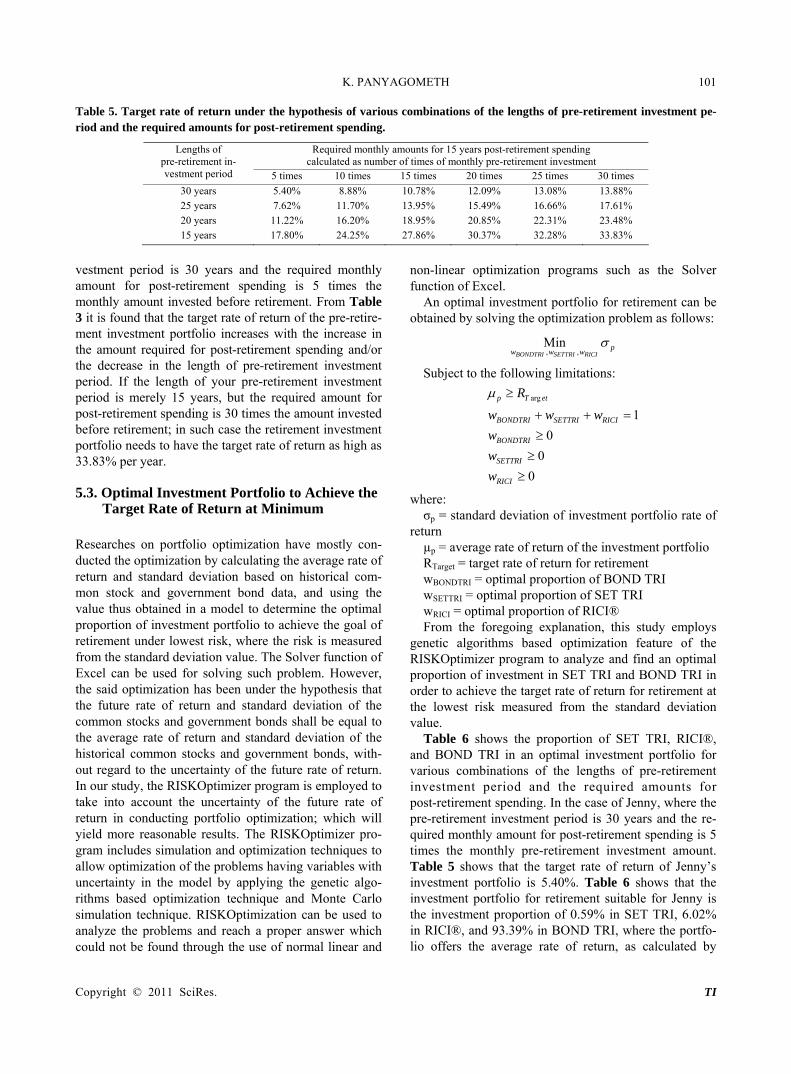
In the case of Jenny who is currently 30 years old and plans to retire at the age of 60; Jenny has a pre-retirement investment period of 30 years. According to the World Health Organization, the average age of Thai men and Thai women are 69 years and 75 years respectively. Therefore, it can be expected that Jenny shall be living another 15 years after retirement. Jenny intends to invest for her retirement the amount of 10,000 Baht at the be-ginning of each month for the next 30 years up to retire-ment. She wishes to earn for post-retirement spending 5 times the amount of pre-retirement investment on monthly basis. In her case the amount is 50,000 Baht. In order to get a conservative estimate, this study was based on the assumption that the post-retirement rate of return was zero. Therefore, Jenny needs to have the total amount of 9,000,000 Baht upon retirement (50,000 Baht per month × 15 years × 12 months per year) in order to be able to withdraw from the sum the monthly amount of 50,000 Baht for 15 years. Based on this assumption, Jenny’s pre-retirement investment portfolio shall have the target rate of return of 0.45% per month or 5.40% per year.

Table 5 shows the target rate of return under various assumptions concerning the length of pre-retirement investment period and the required amount for post-retirement spending. In the case of Jenny, the target rate of return is shown on the top left hand corner of the table, which is the case where the length of pre-retirement in


K. PANYAGOMETH 101 Table 5. Target rate of return under the hypothesis of various combinations of the lengths of pre-retirement investment pe-riod and the required amounts for post-retirement spending.

Required monthly amounts for 15 years post-retirement spending calculated as number of times of monthly pre-retirement investment

Lengths of pre-retirement in-vestment period 5 times 10 times 15 times 20 times 25 times 30 times

30 years 5.40% 8.88% 10.78% 12.09% 13.08% 13.88%

25 years 7.62% 11.70% 13.95% 15.49% 16.66% 17.61%

20 years 11.22% 16.20% 18.95% 20.85% 22.31% 23.48%

15 years 17.80% 24.25% 27.86% 30.37% 32.28% 33.83%

vestment period is 30 years and the required monthly amount for post-retirement spending is 5 times the monthly amount invested before retirement. From Table 3 it is found that the target rate of return of the pre-retirement investment portfolio increases with the increase in the amount required for post-retirement spending and/or the decrease in the length of pre-retirement investment period. If the length of your pre-retirement investment period is merely 15 years, but the required amount for post-retirement spending is 30 times the amount invested before retirement; in such case the retirement investment portfolio needs to have the target rate of return as high as 33.83% per year. 5.3. Optimal Investment Portfolio to Achieve the

Target Rate of Return at Minimum

Researches on portfolio optimization have mostly con-ducted the optimization by calculating the average rate of return and standard deviation based on historical com-mon stock and government bond data, and using the value thus obtained in a model to determine the optimal proportion of investment portfolio to achieve the goal of retirement under lowest risk, where the risk is measured from the standard deviation value. The Solver function of Excel can be used for solving such problem. However, the said optimization has been under the hypothesis that the future rate of return and standard deviation of the common stocks and government bonds shall be equal to the average rate of return and standard deviation of the historical common stocks and government bonds, with-out regard to the uncertainty of the future rate of return. In our study, the RISKOptimizer program is employed to take into account the uncertainty of the future rate of return in conducting portfolio optimization; which will yield more reasonable results. The RISKOptimizer pro-gram includes simulation and optimization techniques to allow optimization of the problems having variables with uncertainty in the model by applying the genetic algo-rithms based optimization technique and Monte Carlo simulation technique. RISKOptimization can be used to analyze the problems and reach a proper answer which could not be found through the use of normal linear and

non-linear optimization programs such as the Solver function of Excel.

An optimal investment portfolio for retirement can be obtained by solving the optimization problem as follows:

, ,Min

BONDTRI SETTRI RICIp

w w w

Subject to the following limitations:

arg

1

0

0

0

p T et

BONDTRI SETTRI RICI

BONDTRI

SETTRI

RICI

R

w w w

w

w

w

where: σp = standard deviation of investment portfolio rate of

return µp = average rate of return of the investment portfolio RTarget = target rate of return for retirement wBONDTRI = optimal proportion of BOND TRI wSETTRI = optimal proportion of SET TRI wRICI = optimal proportion of RICI® From the foregoing explanation, this study employs

genetic algorithms based optimization feature of the RISKOptimizer program to analyze and find an optimal proportion of investment in SET TRI and BOND TRI in order to achieve the target rate of return for retirement at the lowest risk measured from the standard deviation value.

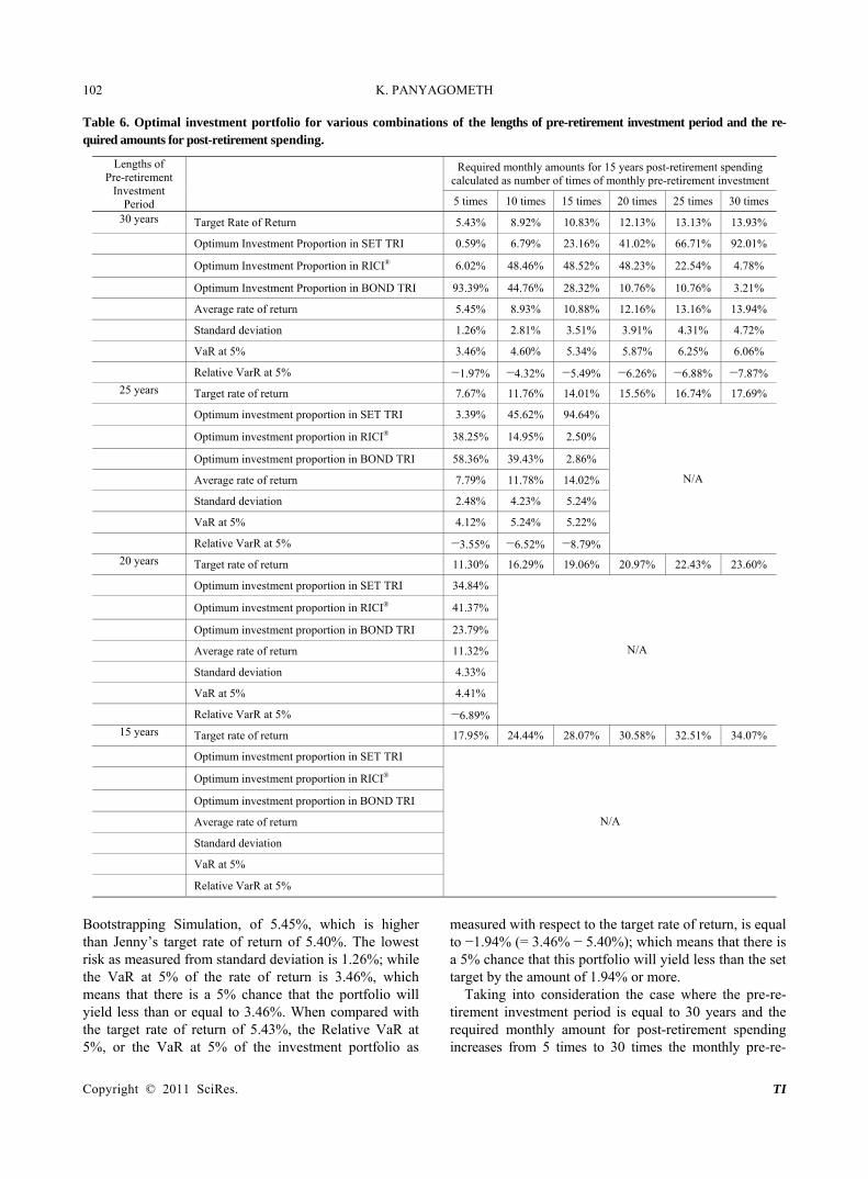
Table 6 shows the proportion of SET TRI, RICI®, and BOND TRI in an optimal investment portfolio for various combinations of the lengths of pre-retirement investment period and the required amounts for post-retirement spending. In the case of Jenny, where the pre-retirement investment period is 30 years and the re-quired monthly amount for post-retirement spending is 5 times the monthly pre-retirement investment amount. Table 5 shows that the target rate of return of Jenny’s investment portfolio is 5.40%. Table 6 shows that the investment portfolio for retirement suitable for Jenny is the investment proportion of 0.59% in SET TRI, 6.02% in RICI®, and 93.39% in BOND TRI, where the portfo-lio offers the average rate of return, as calculated by


K. PANYAGOMETH102 Table 6. Optimal investment portfolio for various combinations of the lengths of pre-retirement investment period and the re-quired amounts for post-retirement spending.

Required monthly amounts for 15 years post-retirement spending calculated as number of times of monthly pre-retirement investment

Lengths of Pre-retirement

Investment Period 5 times 10 times 15 times 20 times 25 times 30 times

30 years Target Rate of Return 5.43% 8.92% 10.83% 12.13% 13.13% 13.93%

Optimum Investment Proportion in SET TRI 0.59% 6.79% 23.16% 41.02% 66.71% 92.01%

Optimum Investment Proportion in RICI® 6.02% 48.46% 48.52% 48.23% 22.54% 4.78%

Optimum Investment Proportion in BOND TRI 93.39% 44.76% 28.32% 10.76% 10.76% 3.21%

Average rate of return 5.45% 8.93% 10.88% 12.16% 13.16% 13.94%

Standard deviation 1.26% 2.81% 3.51% 3.91% 4.31% 4.72%

VaR at 5% 3.46% 4.60% 5.34% 5.87% 6.25% 6.06%

Relative VarR at 5% −1.97% −4.32% −5.49% −6.26% −6.88% −7.87%

25 years Target rate of return 7.67% 11.76% 14.01% 15.56% 16.74% 17.69%

Optimum investment proportion in SET TRI 3.39% 45.62% 94.64%

Optimum investment proportion in RICI® 38.25% 14.95% 2.50%

Optimum investment proportion in BOND TRI 58.36% 39.43% 2.86%

Average rate of return 7.79% 11.78% 14.02%

Standard deviation 2.48% 4.23% 5.24%

VaR at 5% 4.12% 5.24% 5.22%

Relative VarR at 5% −3.55% −6.52% −8.79%

N/A


Optimum investment proportion in SET TRI 34.84%

Optimum investment proportion in RICI® 41.37%

Optimum investment proportion in BOND TRI 23.79%

Average rate of return 11.32%

Standard deviation 4.33%

VaR at 5% 4.41%

Relative VarR at 5% −6.89%

N/A


Optimum investment proportion in SET TRI

Optimum investment proportion in RICI®

Optimum investment proportion in BOND TRI

Average rate of return

Standard deviation

VaR at 5%

Relative VarR at 5%

N/A

Bootstrapping Simulation, of 5.45%, which is higher than Jenny’s target rate of return of 5.40%. The lowest risk as measured from standard deviation is 1.26%; while the VaR at 5% of the rate of return is 3.46%, which means that there is a 5% chance that the portfolio will yield less than or equal to 3.46%. When compared with the target rate of return of 5.43%, the Relative VaR at 5%, or the VaR at 5% of the investment portfolio as

measured with respect to the target rate of return, is equal to −1.94% (= 3.46% − 5.40%); which means that there is a 5% chance that this portfolio will yield less than the set target by the amount of 1.94% or more.

Taking into consideration the case where the pre-re-tirement investment period is equal to 30 years and the required monthly amount for post-retirement spending increases from 5 times to 30 times the monthly pre-re-


K. PANYAGOMETH 103 tirement investment amount, Table 6 shows that the op-timal investment proportion in SET TRI increases from 0.59% to 92.01%, and the optimal investment proportion in BOND TRI decreases from 93.39% to 3.21%. How-ever, the optimal investment proportion in RICI® in-creases from 6.02% to 48.52% when the required monthly amount for post-retirement spending increases from 5 times to 15 times the monthly pre-retirement in-vestment amount and decreases to 4.78% when the re-quired monthly amount for post-retirement spending increases to 30 times the monthly pre-retirement invest-ment amount. Regarding the risk measured from stan-dard deviation, it increases from 1.26% to 4.72% and the risk measured from the Relative VaR at 5% of the rate of return is reduced from −1.94% to −7.82%. For other lengths of pre-retirement investment period, the out-comes are similar to the case where the pre-retirement investment period is 30 years; that is, when the required monthly amount for post-retirement spending increases, the investment proportion in SET TRI in the optimal investment portfolio for retirement shall also increase, which results in higher risk of the investment portfolio.

In the case where the required monthly amount for post-retirement spending is equal to 5 times and the length of pre-retirement investment period is reduced from 30 years to 20 years, Table 6 shows that the opti-mal investment proportion in SET TRI increases from 0.59% to 34.84%, and the optimal investment proportion in RICI® increases from 6.02% to 41.37%, while the optimal investment proportion in BOND TRI decreases from 93.39% to 23.79%. When considering the risk, standard deviation increases from 1.26% to 4.33% and the risk measured from the Relative VaR at 5% of the rate of return is reduced from −1.94% to −6.81%. For other required monthly amounts for post-retirement spending, Table 6 demonstrates the benefit of time di-versification; that is, while the pre-retirement investment period is longer, the risk of the investment portfolio for retirement is reduced. In addition, Table 6 also shows that the goal of required amount for post-retirement spending might not be achieved if the pre-retirement investment period is not long enough. For example, if the pre-retirement investment period is 25 years, but the re-quired monthly amount for post-retirement spending is 20 times the monthly pre-retirement investment amount; in such case the portfolio is required to offer a target re-turn of 15.49%, which is not achievable even with 100% investment in SET TRI due to the fact that the average return of SET TRI is 14.18% as exhibited in Table 4. In case the pre-retirement investment period is 20 years, the goal of having the monthly amount for post-retirement spending as large as 10 times the monthly pre-retirement investment amount is not achievable. While our pre-re-

tirement investment period is reduced to only 15 years, we will not be able to reach the goal of having the monthly amount for post-retirement spending even as low as 5 times the monthly pre-retirement investment amount. 6. Summary Through the use of Bootstrapping Simulation technique in modeling long-term rate of returns based on various combinations of the lengths of retirement investment period and the required amounts for post-retirement spending, this research was conducted to find an optimal proportion of common stocks, commodities and govern-ment bonds to achieve the target rate of return for re-tirement by minimizing investment portfolio risk meas-ured from standard deviation value. Also included was risk analysis based on the Value at Risk concept for studying downside risk of the investment portfolio for retirement. The study has found that in an optimal port-folio for retirement, the proportion of investment in SET TRI becomes smaller, resulting in a corresponding de-crease of portfolio risk, as the length of pre-retirement investment period increases and/or the required amount for post-retirement spending decreases. Furthermore, this study reveals that the longer the period of pre-retirement investment, the lower is the risk of the retirement portfo-lio due to the effect of time diversification, and the larger is the receivable amount for post-retirement spending.

This research reflects that the government should con-duct a publicity campaign to make the Thai society per-ceive the importance of long-term investment, by en-couraging working-age citizens to invest for retirement early so as to have longer pre-retirement investment pe-riod, which shall in turn reduce the risk of retirement portfolio to acceptable level, and to make available the anticipated amount for post-retirement spending. If this could be realized, the government burden with regard to provision of welfare for retired citizens in the future shall be well relieved. 7. References

[1] R. A. Levy, “Stocks, Bonds, Bills, and Inflation over 52 Years,” The Journal of Portfolio Management, Vol. 4, No. 4, 1978, pp. 18-19. doi:10.3905/jpm.1978.408655

[2] W. Reichenstein, “When Stock is Less Risky than Treas-ury Bills,” Financial Analysts Journal, Vol. 42, No. 6, 1986, pp. 71-75. doi:10.2469/faj.v42.n6.71

[3] M. L. Leibowitz and T. C. Langetieg, “Shortfall Risk and the Asset Allocation Decision: A Simulation Analysis of Stock and Bond Risk Profiles,” The Journal of Portfolio Management, Vol. 16, No. 1, 1989, pp. 61-68. doi:10.3905/jpm.1989.409236


http://dx.doi.org/10.3905/jpm.1978.408655

http://dx.doi.org/10.2469/faj.v42.n6.71


K. PANYAGOMETH


104

[4] C. K. Butler and D. L. Domian, “Long-Run Returns on Stock and Bond Portfolios: Implications for Retirement Planning,” Financial Services Review, Vol. 2, No. 1, 1993, pp. 41-49. doi:10.1016/1057-0810(92)90014-4

[5] H. Bjorn and M. Persson, “Time Diversification and Es-timation Risk,” Financial Analysts Journal, Vol. 56, No. 5, 2000, pp. 55-62. doi:10.2469/faj.v56.n5.2390

[6] N. Strong and N. Taylor, “Time Diversification: Empiri-cal Tests,” Journal of Business Finance & Accounting, Vol. 28, No. 3-4, 2001, pp. 263-302. doi:10.1111/1468-5957.00374

[7] K. Hickman, H. Hunter, J. Byrd, J. Beck and W. Terpen-ing, “Life Cycle Investing Holding Periods and Risk,” The Journal of Portfolio Management, Vol. 27, No. 2, 2001, pp. 101-111. doi:10.3905/jpm.2001.319796

[8] C. Gollier, “Time Diversification, Liquidity Constraints, and Decreasing Aversion to Risk on Wealth,” Journal of Monetary Economics, Vol. 49, No. 7, 2002, pp. 1439- 1459.

[9] T. S. Howe and D. L. Mistic, “Taxes, Time Diversifica-tion, and Asset Choice at Retirement,” Journal of Eco-

nomics and Finance, Vol. 27, No. 3, 2003, pp. 404-421. doi:10.1007/BF02761574

[10] B. Guo and M. Darnell, “Time Diversification and Long-Term Asset Allocation,” The Journal of Wealth Management, Vol. 8, No. 3, 2005, pp. 65-76. doi:10.3905/jwm.2005.598423

[11] S. Mukherji, “A Study of Time Diversification with Block Bootstraps and Downside Risk,” The Business Re-view, Vol. 10, No. 1, 2008, pp. 55-60.

[12] L. Alles, “The Cost of Downside Protection and the Time Diversification Issue in South Asian Stock Markets,” Ap-plied Financial Economics, Vol. 18, No. 10, 2008, p. 835. doi:10.1080/09603100701222333

[13] K. Panyagometh, “The Earlier You Invest, the Lower Probability of Ruin You Will Get,” Competitiveness Re-view by NIDA Business School, in Thai, Vol. 1, No. 4, 2009, pp. 75-85.

[14] K. Singh, “On the Asymptotic Accuracy of Efron’s Boot-strap,” Annals of Statistics, Vol. 9, 1981, pp. 1187-1195. doi:10.1214/aos/1176345636

http://dx.doi.org/10.1016/1057-0810(92)90014-4

http://dx.doi.org/10.2469/faj.v56.n5.2390

http://dx.doi.org/10.1111/1468-5957.00374


http://dx.doi.org/10.1007/BF02761574

http://dx.doi.org/10.3905/jwm.2005.598423

http://dx.doi.org/10.1080/09603100701222333

http://dx.doi.org/10.1214/aos/1176345636

asset allocation, time diversification and portfolio ...asset allocation, time diversification and...

Documents