assessment of whiteness and tint of fluorescent...

Rolf Griesser Application Technology Ciba-Geigy Ltd. Basle, Switzerland

Assessment of whiteness and tint of fluorescent substrates with good inter-instrument correlation

Given in English Language at „1994 Williamsburg Conference on Colorimetry of Fluorescent Materials“; English first publication in Color Res. Appl. 19 (1994), 6, p. 446-460; German second publication in Wochenblatt für Papierfabrikation 123 (1995), 18, p. 814-819 und 19, p. 852-855. Abstract and introduction White is primarily a sensation like blue, green, or red and, as such, is not measurable directly. Only a physical property, the spectral reflectance of a sample, can be measured directly. But this is not a standard, fixed quan-tity; it depends on a number of individual properties of the measuring instrument used. The entire geometry of the illuminating chamber - generally speaking a sphere is used for samples with a structured surface - is incor-porated in the measuring results. The size of the aperture and the exclusion or inclusion of gloss also influence reflectance. High whiteness is obtainable only with the aid of fluorescent whitening agents (FWAs), and is hence a fluorescent color, which demands specific qualities of the illumination. The sample illumination must be identical with that for which the colorimetric values have been calculated. Nowadays, however, this is usually standard illuminant D65, which can be simulated only approximately in measuring instruments. In addition, all lamps used are subject to changes in spectral energy distribution. The problem is how to obtain constant, comparable results, namely whiteness, tint, and lightness for fluorescent materials using measuring instruments of different designs incorporating different means of simulating standard illuminant D65 or other D illuminants. This article presents a method that has been in use in industry for about 20 years. The method in question comprises two parts: first, on the hardware side, sample illumination that has to meet specific requirements, match the UV excitation required, and remain stable; second, on the software side, the two critical dimensions whiteness and tint are calculated only indirectly from the measuring results. Only in this way is it possible to achieve a large measure of comparability between different instruments. In principle, the method is also suitable for different illuminants and for any white preference. In all other methods of assessment the parameters are not matched to the instrument characteristics. If the results obtained with different measuring instruments are to be compared, difference values have to be used, entailing the need for standards and involving all the drawbacks associated with them. Key words: instrumental whiteness assessment, transfer standard, white scale, illumination check sample, UV calibrating device, stable illumination, whiteness, tint deviation, instrument-specific formula parameters, inter-instrument agreement, UV excitation, standard illuminant D65, fluorescence, computer programming. Problems with fluorescent whites All the older formulas like those of Hunter, Stensby, Berger, Taube, etc., are for purely one-dimensional evaluations (scalar) 1,2. As for all other colors, however, three dimensions are needed to characterize fluorescent whites unambiguously, e.g. - X, Y, Z or x, y, Y or λd, pe (Helmholtz), Y in the CIE 1964 color order system (DIN

5033),

Rolf Griesser/griesser_paper_williamsburg_1994.doc

2

- L*, a*, b* in the CIELab 1976 color order system (DIN 6174), - whiteness (Ganz), tint deviation (Ganz/Griesser), Y (CIE) in the Ganz/Griesser method, - whiteness, tint in the CIE method (Y not specified but feasible). In many cases, however, there is no need to specify lightness, for example when identical or closely similar substrates are being compared. - With all substrates different measuring instrument designs and - with fluorescent substrates different illumination systems usually lead to results that are not comparable. Apertures of different sizes, the inclusion or exclusion of gloss, illuminants that change over time, and the widely different lamps available impair the comparability of the results obtained with a given instrument.

Principle Problems

- Different designof the measuringinstruments

- Different aperturesizes with one andthe same instrument

- Exclusion orinclusion of gloss

differentinstruments

DCI SF500

Zeiss RFC3

TRF

Wavelength in nm

Eab* = 2.7

Zeiss RFC3

30

155

aperturein mm

TRF

Wavelength in nm

Eab* = 0.5

Eab* = 2.0

Zeiss RFC3specular :

excluded

included

TRF

Wavelength in nm

Eab* = 1.4

0.1

0.6

1.1

1.6

360 400 450 500 550 600 650 700

0.1

0.8

1.5

360 400 450 500 550 600 650 7000.10

0.75

1.40

360 400 450 500 550 600 650 700 FIG. 1. Principle problems.

UV adjustment of the sample illumination Fig. 2 shows the effect of too strong and too weak UV excitation on a fluorescent whitened substrate with a nominal whiteness of 215. The UV calibrator (Gaertner/Griesser) 3,4 influ-ences the ratio of the energy in the UV region to that in the visible region of the spectrum by means of a UV adjustment filter with a steep absorption slope at about 400 nm (Fig. 3). It decisively improves the agreement of the illumination between different measuring instru-


3

ments and performs a useful function in the evaluation of fluorescent substrates by all meth-ods. The lamps used must be similar to the CIE standard, e.g., xenon lamps (for continuous or intermittent illumination) for standard illuminant D65. When new they must emit excess UV radiation and, to avoid over-frequent lamp replacement, this excess must not decrease at too fast a rate. The UV calibrator is fitted as standard in various makes of spectrophotometer. With flash tubes the illumination intensity must not exceed a given magnitude. Otherwise, with a number of FWAs and a few dyes applied at very low concentrations, the triplet effect

TRF C too much UV

B UV according to daylight

A too little UV

Trist. value X

Trist. value Y

Trist. value Z

Whiteness (Ganz)referred to theHohenstein white scale

Meast. A

90.9

94.7

113.9

169

Meast. B

93.0

96.2

123.7

214

Meast. C

94.0

96.9

128.6

236

0.0

0.5

1.0

1.5

wavelength in nanometers350 400 450 500 550 600 650 700

FIG. 2. A substrate measured with too little, the right amount, and too much UV excitation.

Vmixed radiation

sample

integrating sphere

UV-free radiation

xenon lamp

UV-rich radiation

UV-absorbing

filter(400 nm)

FIG. 3. UV calibrating device (Gaertner/Griesser).


4

XENON lamps :continuous burning ____

andflash bulbs - - - -

W = 165 TV = 2.3 = G2( visually confirmed ! )

W = 179 TV = -3.7 = R4( wrong ! )

Uvitex EBF on polyester wavelength in nm0.0

0.1

0.2

0.3

0.4

0.5

0.6

0.7

0.8

0.9

1.0

1.1

1.2

360 380 400 420 440 460 480 500 520 540 560 580 600 620 640 660 680 700 FIG. 4. The flash bulb's triplet effect simulates a non-existent tinting dye.

can occur so markedly as to distort measurement. Studies along these lines have been carried out to date only empirically. We still lack unambiguous physical definition of flash tubes with reference to this effect. The difference between the two assessments of the tint deviation in Fig. 4 is 6 TV units. This is about ten times the distinguishing threshold. Cotton white scales as transfer standards Transfer standards, e.g., cotton white scales marked with nominal values for whiteness and tint value, are used as a rule as a means of transferring illumination conditions from an in-strument for absolute measurement (e.g., PTB, Braunschweig, for non-fluorescent and BAM, Berlin, for fluorescent reference standards) to a reference instrument (e.g., in Ciba or Ho-henstein) and from this to a working / industrial instrument (e.g., in a paper mill) (Table I). Direct measurement of the spectral energy distribution of the illumination at the substrate location would be very cumbersome. A white scale must consist of equal perceptual steps of white, i.e., the differences between the nominal whiteness values must match the visually perceived differences. It should represent a whiteness perceived as roughly neutral but with no implication of quality judgment. Also its spectral properties should resemble as closely as possible those of the samples to be measured, because the sample illumination in measuring instruments differs to a greater or lesser extent from the standard illuminants used for the cal-culations.


5

TABLE I. Cotton white scale as standard for transferring: illumination conditions and the two grids for assessing whiteness and tint deviation

from an instrument yielding absolute CIE tristimulus values

to a reference instrument, and from a reference instrument to a working instrument

The scale mentioned here is made with a widely used dianilino-dimorpholino-triazinyl-stilbene FWA (C.I. Flu Bri 339) on fully bleached cotton. Closely similar in spectral properties to modern textiles and paper, it can be obtained from the manufacturer, Hohenstein Institute, 74357 Boennigheim, Germany. If properly stored it remains effective and can be used for about 3 months. In principle it is intended for just a one-off procedure, namely to establish the method here described for a given measuring instrument. This starting procedure should be repeated only if a lamp with a different spectral energy distribution is fitted. Illumination Check samples Stable, white, fluorescent plastic samples are used to keep the set illumination conditions constant as lamps change (age) or are replaced. These samples, e.g., those available from the Hohenstein Institute, have defined measuring points and are both washable and long-lasting. Individual phases of the method The introduction and subsequent use of the instrumental method of evaluating fluorescent white substrates described here comprises the following individual phases: 1. Determining the preferences and scaling for the whiteness formula (Ganz) and the tint

deviation formula (Ganz/Griesser). Standard values are used as a rule. Determining the whiteness formula parameters for precisely the illuminant or observer desired, e.g., D65/10°.

2. Determination by, for example, BAM, Berlin of the absolute radiance factor of a 4-step

cotton white scale used as a fluorescent transfer standard. Calculation of true tristimulus values for the desired illuminant/observer. The standard is neutral by definition, i.e., the straight line through the scale steps indicates zero tint deviation.

3. Calculating the nominal whiteness (Ganz) of the scale steps from the absolute CIE tris-

timulus values and the above formula for precisely D65/10°. 4. Determining the nominal tint deviation (Ganz/Griesser) of the scale steps from the

straight line through the 4 steps and of the standard value for the scaling.


6

5. Absolute calibration and adjustment of a reference instrument by means of the certified transfer standards and by the UV calibrator (Gaertner/Griesser). Basic calibration is performed beforehand with a non-fluorescent reference standard, e.g., BaSO4 from PTB Braunschweig, Germany, with the perfect diffuser as reference standard. Determining the formula parameters and nominal values valid for the reference instrument from the relative tristimulus values, i.e., slightly different from the absolute values, for the scale measured with this instrument, from the previously calculated nominal value for white-ness and tint deviation, and from the standard value for the UV excitation intensity. The parameters and nominal values now valid for the reference instrument generally differ slightly from those for the ideal illuminant.

6. Determining the nominal values of a plastic sample used to check the optimized illumi-

nation conditions for the reference instrument when the lamp changes (ages) or is re-placed, and to keep them constant by means of the UV calibrator.

7. Determining the nominal values for whiteness and tint deviation of cotton white scales

used as standards to transfer the illumination conditions of the reference instrument to working instruments.

8. Adapting the illumination, calculating instrument-specific formula parameters, and de-

termining illumination check samples for the working instrument using a similar procedure to that for the reference instrument. This phase is to be performed by the industrial user or by the producer of the instrument.

9. Periodic checking of the illumination conditions for both reference and working instru-

ments. The representative numerical data used in the calculations below enable computer programs based on them to be checked for errors. Whiteness formula for precise illuminant/observer For an illumination exactly matching standard illuminant D65 the whiteness formula parame-ters can be calculated from general and whiteness-specific standard given values (all calculations in radians) 4,5,6,7,8,9,10 : RWL = 470 nm Reference dominant wavelength. xd = 0.1152 } Point of intersection of the RWL with the spectrum locus, yd = 0.1090 } dependent on the observer, but not on the illuminant. Xn = 94.81 } Tristimulus values for Yn = 100 } standard illuminant D65 and Zn = 107.33 } CIE 1964 standard observer. xn = Xn / ( Xn + Yn + Zn ) = 0.313795 } Coordinates of the yn = Yn / ( Xn + Yn + Zn ) = 0.330972 } achromatic point. η = atan [ ( yn - yd ) / ( xn - xd ) ] = 48.18154° = 0.84093 (radians) = angle between RWL and x-axis of chromaticity chart.


7

The formula's "white flavor" , that is the contributions of hue, saturation and lightness to the whiteness, is defined by the following values: ϕ = 15° = 0.26180 (radians) Hue preference, referred to the perpendicular to the RWL. δW / δY = 1 Contribution of lightness to whiteness. δW / δS = 4000 Contribution of saturation to whiteness. W0 = 100 Degree of whiteness of physical ideal white.

.0

.1

.2

.3

.4

.5

.6

.7

.8

.9

.0 .2 .4 .6 .8

y

xη

RWL 470 nm

White Scaleϕ

FIG. 5. Chromaticity chart D65/10° with RWL = 470 nm, its perpendicular and the angle ϕ = 15°.

From these standard values can be calculated the formula parameters D, P, Q, C: D = δW / δY = 1 (1) P = ( -δW / δS ) * ( cos ( ϕ + η ) / cos ( ϕ )) = -1868.322 (2) Q = ( -δW / δS ) * ( sin ( ϕ + η ) / cos ( ϕ )) = -3695.690 (3) C = [ W0 * ( 1 - δW / δY )] - ( P * xn ) - ( Q * yn ) = 1809.441 (4) W (Ganz) = ( D * Y ) + ( P * x ) + ( Q * y ) + C (5) Fig. 5 shows at bottom left the angle η, formed by the RWL and the x-axis. The 4 squares at the upper end of the RWL covering the achromatic point represent the 4 steps of a cotton white scale. Further equations in the context of the contributions of hue and saturation to whiteness are: δW / δH = -δW / δS * tan ( ϕ ) (6) S = ( tan ( ψ ) * (xn - x ) - ( yn - y )) / ( tan ( ψ ) * cos ( η ) - sin ( η )) (7) ψ = ϕ + η + π / 2 (8)


8

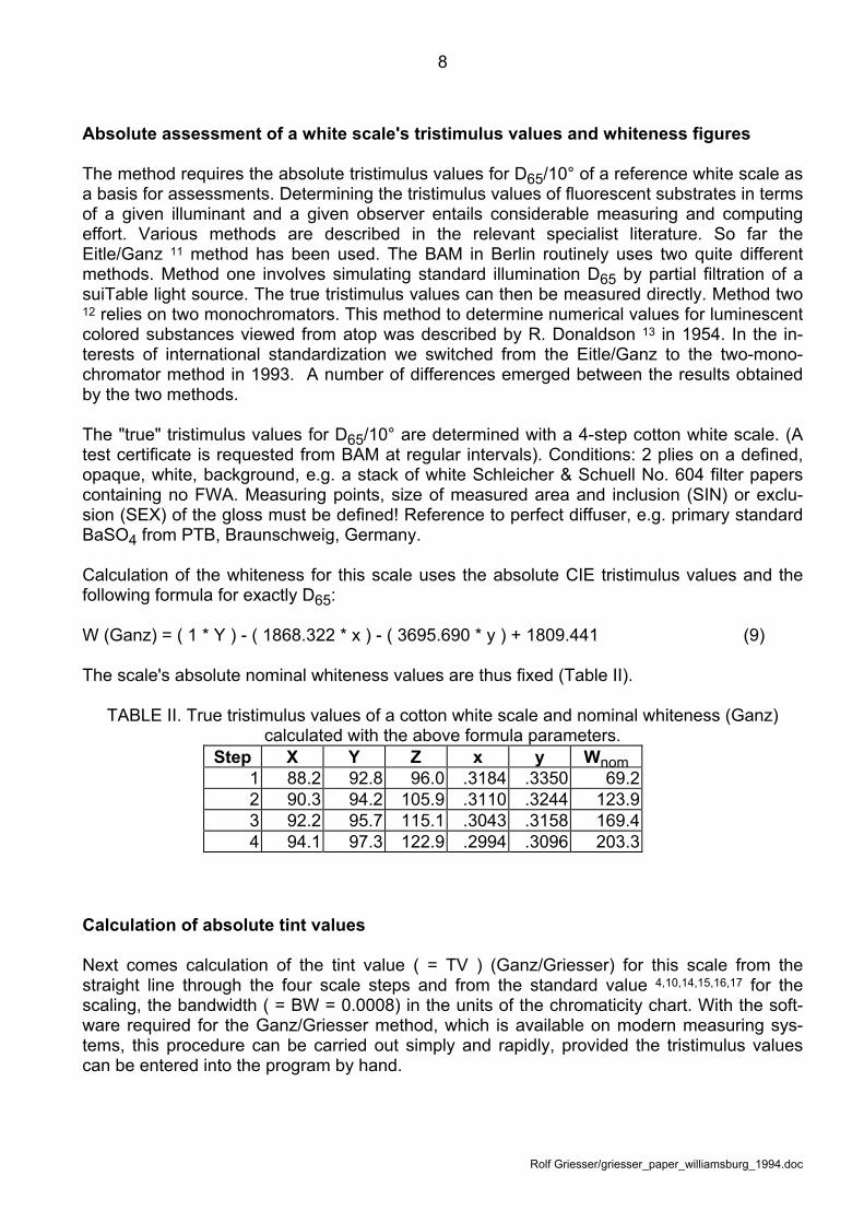
Absolute assessment of a white scale's tristimulus values and whiteness figures The method requires the absolute tristimulus values for D65/10° of a reference white scale as a basis for assessments. Determining the tristimulus values of fluorescent substrates in terms of a given illuminant and a given observer entails considerable measuring and computing effort. Various methods are described in the relevant specialist literature. So far the Eitle/Ganz 11 method has been used. The BAM in Berlin routinely uses two quite different methods. Method one involves simulating standard illumination D65 by partial filtration of a suiTable light source. The true tristimulus values can then be measured directly. Method two 12 relies on two monochromators. This method to determine numerical values for luminescent colored substances viewed from atop was described by R. Donaldson 13 in 1954. In the in-terests of international standardization we switched from the Eitle/Ganz to the two-mono-chromator method in 1993. A number of differences emerged between the results obtained by the two methods. The "true" tristimulus values for D65/10° are determined with a 4-step cotton white scale. (A test certificate is requested from BAM at regular intervals). Conditions: 2 plies on a defined, opaque, white, background, e.g. a stack of white Schleicher & Schuell No. 604 filter papers containing no FWA. Measuring points, size of measured area and inclusion (SIN) or exclu-sion (SEX) of the gloss must be defined! Reference to perfect diffuser, e.g. primary standard BaSO4 from PTB, Braunschweig, Germany. Calculation of the whiteness for this scale uses the absolute CIE tristimulus values and the following formula for exactly D65: W (Ganz) = ( 1 * Y ) - ( 1868.322 * x ) - ( 3695.690 * y ) + 1809.441 (9) The scale's absolute nominal whiteness values are thus fixed (Table II).

TABLE II. True tristimulus values of a cotton white scale and nominal whiteness (Ganz) calculated with the above formula parameters.

Step X Y Z x y Wnom 1 88.2 92.8 96.0 .3184 .3350 69.2 2 90.3 94.2 105.9 .3110 .3244 123.9 3 92.2 95.7 115.1 .3043 .3158 169.4 4 94.1 97.3 122.9 .2994 .3096 203.3

Calculation of absolute tint values Next comes calculation of the tint value ( = TV ) (Ganz/Griesser) for this scale from the straight line through the four scale steps and from the standard value 4,10,14,15,16,17 for the scaling, the bandwidth ( = BW = 0.0008) in the units of the chromaticity chart. With the soft-ware required for the Ganz/Griesser method, which is available on modern measuring sys-tems, this procedure can be carried out simply and rapidly, provided the tristimulus values can be entered into the program by hand.


9

TABLE III. Calculation of the parameters m, n, k from the chromaticity coordinates x, y of a cotton white scale, consisting of 4 steps:

step = i xi yi group x- y- TVnom 1 .3184 .3350 I .3184 .3350 0.18 2 .3110 .3244 II .3110 .3244 -0.31 3 .3043 .3158 .3043 .3158 -0.04 4 .2994 .3096 III .2994 .3096 0.18 average I - III .3083 .3212

Straight lines have been fitted using the Bartlett method 18, which does not need the as-sumption of no error in the x-values, as would be the case in the usual linear regression situation. Following the Bartlett method, here the data are divided into 3 groups. Group I = group III = int ( i / 3 ) = 1. In this example groups I and III consist only of single figures. b = slope of the line = ( y-III - y-I ) / ( x-III - x-I ) = ( 0.3096 - 0.3350 ) / ( 0.2994 - 0.3184 ) = 1.33788 (10) α = atan ( 1 / b ) = atan ( 1 / 1.33788 ) = 0.64187 (11) m = -cos ( α ) / BW = -cos ( 0.64187 ) / 0.0008 = -1001.223 (12) n = sin ( α ) / BW = sin ( 0.64187 ) / 0.0008 = 748.366 (13) k = -m * x- - n * y- = 1001.223 * 0.3083 - 748.366 * 0.3212 = 68.261 (14) TVnom (Ganz/Griesser) = m * x + n * y + k (for results see Table III.) (15)

TABLE IV. Corresponding Tint Values and Tint Deviations and their coloristic meanings. TV TD coloristic meaning

< -5.5 RR tinted in red direction -5.5 to -4.51 R5 very markedly } -4.5 to -3.51 R4 markedly } redder than -3.5 to -2.51 R3 appreciably } -2.5 to -1.51 R2 slightly } the white scale -1.5 to -0.51 R1 trace } -0.5 to 0.49 no appreciable

deviation in tint from the white scale

0.5 to 1.49 G1 trace } 1.5 to 2.49 G2 slightly } greener than 2.5 to 3.49 G3 appreciably } 3.5 to 4.49 G4 markedly } the white scale 4.5 to 5.49 G5 very markedly }

5.5 GG tinted in green direction The absolute nominal tint values of the scale, valid for exactly D65, are thus fixed. The TVs of the scale steps should vary by not more than ±0.5 from zero. For interpretation see Table IV. The type of graph in Fig. 6 is a very convenient way to show tint deviation and whiteness to-gether.


10

FIG. 6. Showing tint deviation = red/green axis and whiteness = yellow/blue axis.

For fundamental studies, e.g., for fixing production control tolerance limits, it can be expedi-ent to be able to calculate the colorimetric characteristics of theoretical substrates defined in terms of W, TV and Y. This of course calls for the formula parameters D, P, Q, C, m, n, k. The following equations show how the calculations are performed. A, B, R are only interme-diate values. A = W - D * Y - C (16) B = TV - k (17) R = P * n - Q * m (18) x = ( 1 / R ) * ( A * n - B * Q ) (19) y = ( 1 / R ) * ( B * P - A * m ) (20) X = x * Y / y (21) Z = ( 1 - x - y ) * Y / y (22) Fitting the lighting conditions of a reference instrument and calculation of instrument-specific formula parameters The white scale is measured on the reference instrument and the relative tristimulus values for D65/10° are calculated. The parameters D, P, Q, C and the characteristic ðW/ðS are de-termined for the whiteness formula. For the tint deviation formula the parameters m, n, k are calculated. In both cases the relative tristimulus values, the absolute nominal values for W, and the standard value for the bandwidth are used for the calculation. ðW/ðS must equal 4000±10. Too high a value for ðW/ðS means too low UV excitation and vice versa. To find the right value, the position of the UV calibrator (Gaertner/Griesser) 3 may have to be altered several times and the scale remeasured after each alteration. For large changes in the UV calibrator's position, the basic calibration versus black and white may have to be repeated, depending on the design of the measuring instrument. Aim of procedure: to achieve metameric D65 illumination. The degree of this metamerism depends on the type of illumina-tion in the reference instrument.


11

TABLE V. Data for the calculation of formula parameters for the reference instrument. step = i X Yi Z group xi yi Si* Wi* Wnom TVnom

1 88.052 92.725 95.877 I .3183 .3352 .4961 -23.502 68.1 0.172 90.381 94.132 106.241 II .3108 .3238 .4809 29.745 125.7 -0.233 92.515 95.646 115.256 .3049 .3152 .4694 73.731 169.8 -0.124 93.684 96.376 121.837 III .3004 .3090 .4608 106.898 202.1 0.17 average I - III .3086 .3208 .4768 46.718

Si* = xi * V + yi (23) Wi* = Wi - D * Yi (24) where V = 1 / tan ( ϕ + η ) (25) Wi = nominal whiteness from Table II The straight line is again calculated by Bartlett's method 18 : WI* = W1* WIII* = W3* SI* = S1* SIII* = S3* = average (26) b = Q = ( WIII* - WI* ) / ( SIII* - SI* ) = ( 106.898 - (-23.502) ) / ( 0.4608 - 0.4961 ) = -3702.499 (27) P = Q * V = -3702.499 * 0.50554 = -1871.764 (28) a = C = Wi* - Q * Si* = 46.718 - (-3702.499) * 0.4768 = 1812.058 (29) ðW/ðS = -P * cos ( ϕ ) / cos ( ϕ + η ) = 1871.764 * 0.9659 / 0.4512 = 4007.4 (30) where a and b are the axis section and slope of the line. The whiteness formula parameters last calculated (for which calculation the correct value for ðW/ðS (4007) was given) are now valid for the reference instrument and saved. The instrument-specific parameters m, n, k are then calculated: b = ( y-III - y-I ) / ( x-III - x-I ) = ( 0.3090 - 0.3352 ) / ( 0.3004 - 0.3183 ) = 1.46118 (31) α = atan ( 1 / b ) = atan ( 1 / 1.46118 ) = 0.60016 (32) m = -cos ( α ) / BW = -cos ( 0.60016 ) / 0.0008 = -1031.554 (33) n = sin ( α ) / BW = sin ( 0.60016 ) / 0.0008 = 705.973 (34) k = -m * x- - n * y- = 1031.554 * 0.3086 - 705.973 * 0.3208 = 91.871 (35) Recalculation of the scale's W(nom) and TV(nom) with the measured values and the refer-ence instrument's parameters yields the values listed in the two right-hand columns of Table V, which differ slightly from the original results in Tables II and III. The TVs of the scale steps should not differ from zero by more than ±0.5 unit. Fig. 7 shows an example of an assess-ment grid based on instrument-specific formula parameters using the data in Table V. Immediately afterwards the nominal whiteness values of a very stable, white, fluorescent il-lumination check sample 19, e.g., one of the plastic samples available from the Hohenstein Institute, are measured and determined. The sample is used to check the set illumination conditions after calibration versus black and white and to reinstate them by means of a UV calibrator after lamp changes such as aging have occurred or following lamp replacement.


12

There are two versions with 4 and 10 precisely defined measuring points, respectively, for different sized apertures. They will last for about 5 years if properly used. Separate instruc-tions for use are available.

FIG. 7. Example of a grid for assessing whiteness and tint deviation.

If a type of lamp with different spectral characteristics is fitted, the position of the UV calibra-tor and the instrument-specific formula parameters have to be redetermined, i.e., the afore-mentioned procedure has to be repeated. If the reference instrument is checked as described and its illumination conditions are kept constant, it can be used to determine the Ganz/Griesser nominal whiteness and TVs of fluorescent and non-fluorescent white substrates. The main purpose of such a reference instrument is to determine white scales that can be used to transfer the illumination condi-tions to working instruments. If a user wishes to correlate his results with a different white scale whose absorption and re-flectance characteristics differ markedly from those of the cotton white scale, e.g., the Ciba plastic white scale, the illumination in the working instrument must first be adjusted with a cotton white scale in the manner described earlier. The plastic white scale (Ciba: steps 5-11) is then measured without change to the illumination setting, and its formula parameters are determined. The instrument-specific formula parameters for whiteness and tint deviation of the absolute Ganz/Griesser method largely balance out the remaining differences in the measuring results


13

still left after adaptation of the sample illumination. These differences, which are chiefly design-related, can range fortuitously from insignificant to very marked. The use of instru-ment-specific parameters means that the assessment basis, which is predetermined by the transfer standards with their nominal values, is fixed together with its scaling for each in-strument separately.

Using non-neutral transfer standards If the TVs of the individual steps of a transfer standard determined on a reference instrument are close to zero, the tint deviation grid is transferred without appreciable change of its basis to a working instrument. But if some or all of the TVs differ markedly from zero, redeter-mination of the straight line on the working instrument can introduce distortion if the steps are simply assumed to be neutral. The same problem arises if for some reason a non-neutral transfer standard is deliberately used but the tint assessment basis is to be retained.

FIG. 8. Straight lines of uncorrected and corrected assessment basis.

The problem can be overcome by an additional calculation. It is a wise precaution to integrate this correction into the standard software and use it routinely, because the transfer standard TVs are always known. After measurement of the transfer standard on the working instrument, a theoretical white scale with TV = 0, which then forms the basis of the assess-ment grid for this instrument, is calculated using the TVs found with the reference instrument. The calculation can be demonstrated by an extreme example, a transfer standard comprising 4 steps of a plastic white scale, all considerably greener than the tint assessment basis of the reference instrument. Fig. 8 shows the straight line of the reference instrument (continuous line) and the 4 markedly greener steps of a plastic white scale (dots). If the scale is measured


14

on the working instrument, the results (circles) differ to varying degrees as a rule. If, on the assumption that the scale is neutral, a new straight line is determined for the working instrument, the dotted line is obtained. The circles lie very close to this line. On recalculation with the new formula parameters, the scale steps have TVs that are close to zero. The aim, therefore, is to determine a straight line from which the working instrument's measured values and those of the reference instrument are equidistant, indicating that the TVs are the same. The broken line was obtained by the calculations below. Fig. 9 is an enlargement of the small rectangular area in Fig. 8.

TABLE VI. Formula parameters from the reference instrument. D P Q C m n k 1 -1886.3 -3729.0 1832.6 -1006.1410 741.7408 71.8934

TABLE VII. Measuring results from the working instrument and nominal figures from the

reference instrument. step X Y Z x y Wnom TVnom Si* Wi* group

1 81.696 86.628 91.070 .3149 .3340 78.7 2.63 .49318 -7.928 I 2 83.316 87.769 97.183 .3106 .3272 113.2 2.30 .48417 25.431 II 3 83.880 87.595 103.045 .3056 .3191 151.4 1.78 .47355 63.805 II 4 86.025 89.214 113.358 .2981 .3091 202.4 2.47 .45982 113.186 III

First, the formula parameters for the working instrument are calculated from the nominal val-ues of the reference instrument (Table VII) as outlined in the foregoing chapter and again using the Bartlett method. This calculation yields the uncorrected parameters given in Table VIII.

TABLE VIII. Uncorrected formula parameters from the working instrument. D P Q C m n k 1 -1835.3096 -3630.3892 1782.7989 -1033.9869 702.4039 91.3210

Next, a theoretical white scale is calculated. Theoretical chromaticity coordinates are calcu-lated from the measured coordinates. The TVs are the nominal values of the reference in-strument, BW is the standard bandwidth, ϕ the standard hue preference, m and n are the uncorrected parameters from Table VIII.


15

Regression lines: Working instrument Reference instr. Working instr.(uncorrected) (corrected)

x

y

yt

x xt

d

cb

e

y

.3075

.3080

.3085

.3090

.3095

.3100

.2970 .2975 .2980 .2985 .2990 .2995 .3000 .3005 FIG. 9. Calculation of xt and yt.

x, y = step 4 (working instrument) with TV = 2.47 xt, yt = step 4 (theor. white scale) with TV = 0 α = atan ( n / -m ) (36) β = 90 - α (37) δ = 90 - β - ϕ (38) xt = x + d (39) d = c * cos ( δ ) (40) c = b / cos ( ϕ ) (41) b = TV * BW (42) yt = y - e (43) e = c * sin ( δ ) (44) xt = x - ( -TV * BW / cos ( ϕ )) * cos ( α - ϕ ) (45) yt = y + ( -TV * BW / cos ( ϕ )) * sin ( α - ϕ ) (46)

TABLE IX. Data to determine the corrected formula parameters. step Y xt yt Wnom TVnom Si* Wi* group

1 86.628 .3170 .3332 78.7 0.00 .49351 -7.928 I 2 87.769 .3124 .3265 113.2 0.00 .48446 25.431 II 3 87.595 .3069 .3186 151.4 0.00 .47377 63.805 II 4 89.214 .3000 .3085 202.4 0.00 .46013 113.186 III

The corrected formula parameters are calculated from these data, retaining the Y and W values but using TV = 0 (Table X).

TABLE X. Corrected formula parameters from the working instrument. D P Q C m n k 1 -1834.2257 -3628.2452 1782.8007 -1030.9861 706.8010 91.2739

All values are listed in Table XI for comparison. The whiteness values are affected only very slightly by the correction calculation. But the TVs, after correction, are almost identical with the values determined by the reference instrument whereas, uncorrected and distorted, they are almost neutral.


16

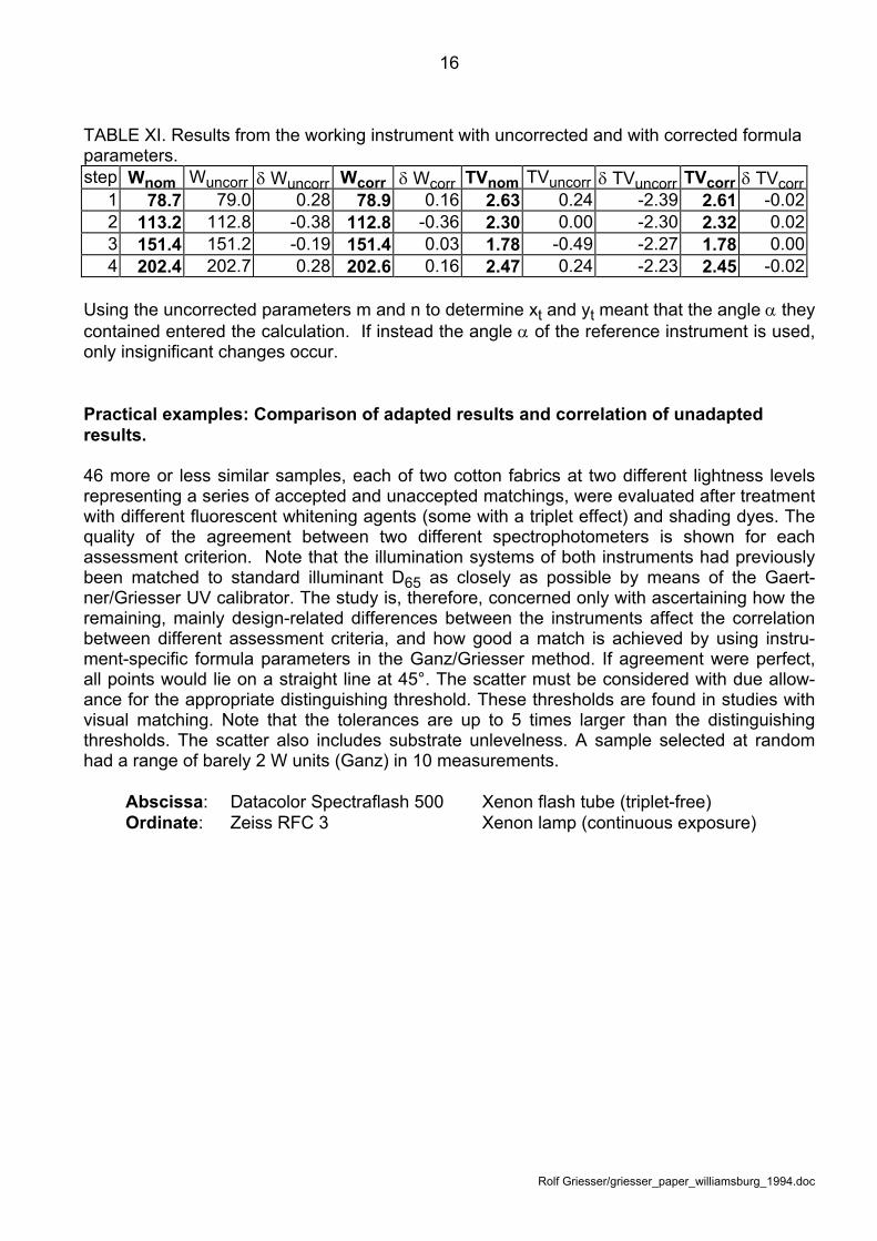
TABLE XI. Results from the working instrument with uncorrected and with corrected formula parameters. step Wnom Wuncorr δ Wuncorr Wcorr δ Wcorr TVnom TVuncorr δ TVuncorr TVcorr δ TVcorr

1 78.7 79.0 0.28 78.9 0.16 2.63 0.24 -2.39 2.61 -0.022 113.2 112.8 -0.38 112.8 -0.36 2.30 0.00 -2.30 2.32 0.023 151.4 151.2 -0.19 151.4 0.03 1.78 -0.49 -2.27 1.78 0.004 202.4 202.7 0.28 202.6 0.16 2.47 0.24 -2.23 2.45 -0.02

Using the uncorrected parameters m and n to determine xt and yt meant that the angle α they contained entered the calculation. If instead the angle α of the reference instrument is used, only insignificant changes occur. Practical examples: Comparison of adapted results and correlation of unadapted results. 46 more or less similar samples, each of two cotton fabrics at two different lightness levels representing a series of accepted and unaccepted matchings, were evaluated after treatment with different fluorescent whitening agents (some with a triplet effect) and shading dyes. The quality of the agreement between two different spectrophotometers is shown for each assessment criterion. Note that the illumination systems of both instruments had previously been matched to standard illuminant D65 as closely as possible by means of the Gaert-ner/Griesser UV calibrator. The study is, therefore, concerned only with ascertaining how the remaining, mainly design-related differences between the instruments affect the correlation between different assessment criteria, and how good a match is achieved by using instru-ment-specific formula parameters in the Ganz/Griesser method. If agreement were perfect, all points would lie on a straight line at 45°. The scatter must be considered with due allow-ance for the appropriate distinguishing threshold. These thresholds are found in studies with visual matching. Note that the tolerances are up to 5 times larger than the distinguishing thresholds. The scatter also includes substrate unlevelness. A sample selected at random had a range of barely 2 W units (Ganz) in 10 measurements. Abscissa: Datacolor Spectraflash 500 Xenon flash tube (triplet-free) Ordinate: Zeiss RFC 3 Xenon lamp (continuous exposure)


17

120

140

160

180

200

220

240

120 140 160 180 200 220 240W (Ganz) (Spectraflash 500)

W (Ganz) (Zeiss RFC3)

Distinguishing threshold: 5 units

FIG. 10. Matching the yellow-blue axis.

-2.00

-1.00

0.00

1.00

2.00

3.00

4.00

5.00

6.00

-2.00 0.00 2.00 4.00 6.00TV (Ganz/Griesser) (Spectraflash 500)

TV (Ganz/Griesser) (Zeiss RFC3)

Distinguishing threshold: 0.5 unit

FIG. 11. Matching the red-green axis.

Assessment with a whiteness formula can be compared approximately with an assessment on the yellow-blue axis in a color system in which chromaticity and lightness both contribute towards the whiteness. Tint assessment in the Ganz/Griesser and CIE 20,21,22,23 methods, however, takes place on the red-green axis. Figs. 10 and 11 show the match obtainable with the instrument-specific formula parameters for W = whiteness (Ganz) and TV = tint value (Ganz/Griesser). Fig. 12 shows the 3rd axis of the Ganz/Griesser method, lightness Y. As evidenced by the low scatter, however, there is no need for matching Y. In this case, the distinguishing threshold is given by δW/δY = D = 1 and the threshold of 5 units for W (Ganz).


18

82

84

86

88

90

92

94

96

82 84 86 88 90 92 94 96Lightness Y (Spectraflash 500)

Lightness Y (Zeiss RFC3)

Distinguishing threshold: 5 units

FIG. 12. Correlation of lightness axis.

90

100

110

120

130

140

150

160

90 100 110 120 130 140 150 160W (CIE) (Spectraflash 500)

W (CIE) (Zeiss RFC3)

Distinguishing threshold: 1.9 units

FIG. 13. Correlation of the yellow-blue axis.

Figs. 13 and 14 show the correlation for whiteness and tint (CIE). No matching is performed here. The formula parameters are the same for both instruments. The scatter for W (CIE) is considerably greater than for W (Ganz), but still satisfactory. Against that, there is a particu-larly marked systematic discrepancy in the CIE tint calculation. The distinguishing thresholds are lower here than in the Ganz/Griesser method, because the scalings differ.


19

-4.00

-3.00

-2.00

-1.00

0.00

1.00

2.00

3.00

4.00

-4.00 -3.00 -2.00 -1.00 0.00 1.00 2.00 3.00 4.00Tint (CIE) (Spectraflash 500)

Tint (CIE) (Zeiss RFC3)


FIG. 14. Correlation of the red-green axis.

The situation is very similar in the CIELab system DIN 6174 (figs. 15 and 16). The red-green axis is invariably the critical one. Only an assessment system that matches this axis can balance out instrument-related differences. This means uncoupling the final results from the measured values and the quantities derived directly from them. It necessitates instrument-specific formula parameters.

-1

0

1

2

3

4

5

-1 0 1 2 3 4 5a* (CIELab) (Spectraflash 500)

a* (CIELab) (Zeiss RFC3)


FIG. 15. Correlation of the red-green axis.


20

-15

-13

-11

-9

-7

-5

-3

-15 -13 -11 -9 -7 -5 -3b* (CIELab) (Spectraflash 500)

b* (CIELab) (Zeiss RFC3)



Finally, Fig. 17 shows evaluation with one of the classical whiteness formulas, with whiteness (Berger) 1,2. If anything, the scatter here is greater than for W (CIE).

90

100

110

120

130

140

150

160

170

90 100 110 120 130 140 150 160 170W (Berger) (Spectraflash 500)

W (Berger) (Zeiss RFC3)

Distinguishing threshold: 2.8 units


Conclusion

The yellow-blue axis (whiteness, b*) is generally less critical, provided the illumination conditions can be optimally matched to standard illumination D65 with the UV calibrator (Gaertner/Griesser). Instrument-specific formula parameters, however, markedly im-prove the correlation. They can also balance out larger differences than those observed with these two spectrophotometers.


21

The red-green axis (TV, tint, a*) shows the instrument differences most markedly. Without instrument-specific formula parameters, evaluation criteria will very rarely be comparable on this axis, at best with instruments of the same series.

The lightness axis is usually not critical. Matching by instrument-specific formula pa-

rameters is not necessary. Finally I would like to thank Mr. R. V. Bathe for his critical review of the statistical calculations and Mr. G. Cameron for his careful rendering of my text into English. REFERENCES 1. A. Berger, Weissgradformeln und ihre praktische Bedeutung, Die Farbe 8 (1959), Nr. 4/6, pp. 187-202. 2. P. Stensby, Optical brighteners as detergent additives, J. Amer. Oil Chem. Soc. 45 (1968), 7, pp. 497-504. 3. F. Gaertner and R. Griesser, A device for measuring fluorescent white samples with constant UV excita-

tion, Translation from Die Farbe 24 (1975) 1/6. pp. 199-207. 4. R. Griesser, Instrumental measurement of fluorescence and determination of whiteness: review and ad-

vances, Review of Progress in Coloration 11 (1981), pp. 25-36. 5. E. Ganz, Whiteness measurement, Journal of Color & Appearance 1 (1972), 5, pp. 33-41. 6. E. Ganz, Whiteness: Photometric specification and colorimetric evaluation, Appl. Opt. 15 (1976), 9, pp.

2039-2058. 7. E. Ganz, Whiteness formulas: a selection, Appl. Opt. 18 (1979), 4, pp. 1073-1078. 8. E. Ganz, Whiteness perception: individual differences and common trends, Appl. Opt. 18 (1979), 17, pp.

2963-2970. 9. E. Ganz, Individual differences in perceiving whiteness, Acta Chromatica 3 (1980), 5, pp. 190-193. 10. R. Griesser, Whiteness not Brightness: a new way of measuring and controlling production of paper, Appita

46 (1993), 6, pp. 439-444. 11. D. Eitle and E. Ganz, Eine Methode zur Bestimmung von Normfarbwerten fuer fluoreszierende Proben,

Textilveredlung 3 (1968), 8, pp. 389-392. 12. D. Gundlach, Die Zwei-Monochromatoren-Methode fuer die Farbmessung an lumineszierenden Proben,

Die Farbe 32/33 (1985/86), pp. 81-125. 13. R. Donaldson, Spectrophotometry of fluorescent pigments, Brit. J. Appl. Phys. 5 (1954), pp. 210-214. 14. E. Ganz and R. Griesser, Whiteness: assessment of tint, Appl. Opt. 20 (1981), 8, pp. 1395-1396. 15. R. Griesser, Status of instrumental whiteness assessment with particular reference to the illumination,

Translation from Textilveredlung 18 (1983), 5, pp. 157-162. 16. J. Rieker and D. Gerlinger, Die farbmetrische Weissbewertung nach Ganz/Griesser, Kongress-Schrift der

SEPAWA e.V. (1985), pp. 39-40. 17. R. Griesser and M. Luria, Valoración instrumental del blanco, Revista de química textil 92 (1988), Octubre-

Diciembre, pp. 74-92. 18. M. S. Bartlett, Fitting a straight line when both variables are subject to error, Biometrics 5 (1949), pp. 207-

212 and Corrigenda: Biometrics 6 (1950). 19. R. Griesser and J. Rieker, Weiss - eine schwierige Farbe!?, Textilveredlung 27 (1992), 10, pp. 339-340. 20. A. Brockes, The evaluation of whiteness, CIE Journal 1 (1982), 2, pp. 38-39. 21. The evaluation of whiteness, Colorimetry Second Edition, CIE Publication No. 15.2 (1986), pp. 36-38. 22. J. A. Bristow, What is ISO brightness? Tappi Journal 77 (1994), 5, pp. 174-178. 23. J. A. Bristow, The Calibration of Instruments for the Measurement of Paper Whiteness, Color Res. Appl. 19

(1994), 6, pp. 475-483.

assessment of whiteness and tint of fluorescent...

Documents