smJoz(30a-@5/74~, % ,Presented at the 23rd Annual Meeting of Adhesion Society, Myrtle Beach, SC, February 23,2000

Assessment of Surface Contamination with Contact MechanicsJohn A. Emerson, Gregory V. Miller, and Christopher R. Sorensen

Sandia National LaboratoriesDepartment of Organic MaterialsAlbuquerque, NM 87185-0958

andRaymond A. Pearson

Lehigh UniversityMaterials Science and Engineering Department

Bethlehem, PA 18015-3195

INTRODUCTION

We are particularly interested in the work of adhesionmeasurements as a means to facilitate our understandingof the adhesive failure mechanisms for systemscontaining encapsulated and bonded components. Of theseveral issues under investigation, one is the effect oforganic contamination on the adhesive strength for

several types of polymer/metal interface combinations.The specific question that we are trying to address is atwhat level of contamination does adhesive strengthdecrease. The use of contact mechanics, the JKRmethod, is a good approach for studying this question.Another approach being studied is the use of interracialfacture mechanics [1]. The model contaminant ishexadecane – non-polar, medium molecular weighthydrocarbon fluid. We choose hexadecane because itreplicates typical machining fluids, is nonreactive withAl surfaces, and should not dissolve readily into theadhesive systems of interest. The application of auniform, controllable and reproducible hexadecane layeron Al surfaces has proven to be dit%cult [2]. A primaryconcern is whether studies of model systems can beextended to systems of technological interest.

The JKR theory is a continuum mechanics model ofcontact between two solid spheres that was developedby Johnson, Kendall and Roberts [3]. The JKR theory isan extension of Hertzian contact theory [4] andattributes the additional increase in the contact areabetween a soft elastomeric hemisphere to adhesiveforces between the two surfaces. The JKR theory allowsa direct estimate of the surface free energy of interfaceas well as the work of adhesion (Wa) between solids.Early studies performed in this laboratory involved thedetermination of Wa between silicone (PDMS) and Alsurfaces in order to establish the potential adhesivefailure mechanisms. However, the JKR studies usingcommercial based PDMS was fraught with difficultythat were attributed to the additives used in commercial

PDMS systems. We could not discriminate hydrogen-bonding effects between A1203 and hydroxyl groups inthe PDMS, and other possible bonding mechanisms. Amodel PDMS elastomer and polymer treatments weredeveloped for studying solid surfaces by measuring thedegree of self-adhesion hysteresis [5] as indicator ofsurface properties.

The goal of this work is to measure the adhesion

between PDMS/Al surfaces – contaminated and twocleaning techniques. A custom-made JKR apparatus isused to determine the amount of hysteresis and Wa.

EXPERIMENTAL

Preparation of PDMS Lens

Model networks of poly(dimethylsiloxane) were

synthesized by reacting vinyl-capped

poly(dimethylsiloxane) with tetrakis (dimethylsiloxy)silane in the presence of a platinum catalyst. The use ofthe platinum – divinyltetramethy ldisiloxane complexallowed the polymerization to proceed at roomtemperature without the formation of by-products. Allreactants were used as received from Gelest Inc.

The procedure used to synthesize the PDMS networks is

fas follows. First, tetrakis ( imethylsiloxy) silane wasadded using an Eppendor volumetric dispenser. Withthe amount of cross-linker fixed, a 0.75 stoichiometric

amount of vinyl-capped PDMS (6000 g/mol) was addedwith a 3 ml syringe. The contents were then mixedthoroughly and stored in a freezer at –20 C. Once thetemperature was low enough to slow the reaction,approximately 150 ppm of platinum –divinyltetramethy ldisiloxane complex was worked intothe system. Hemispheres, which are used as the JKR[ens, were prepared using an oiler (medium, DL-32).

Drops of the mixture were placed on tridecaflro- 1,1,2,2-tetrahydroctyl trichlorosilane treated glass surface.

Issued by Sandia National Laboratories, operated for the United States Depart-merit ofEnergy by Sandia Corporation.

NOTICE: This report was prepared as an account of work sponsored by an agency of theUnited States Government. Neither the United States Govem-ment, nor any agencythereof, nor my of their employees, nor any of their contractors, subcontractors, or theiremployees, make any warranty, express or implied, or assume any legal liability orresponsibility for the accuracy, completeness, or usefulness of any information, apparatus,product, or process disclosed, or represent that its use would not infringe privately ownedrights. Reference herein to any specific commercial product, process, or service by tradename, trademark, manufacturer, or otherwise, does not necessarily constitute or imply itsendorsement, recommendation, or favoring by the United States Government, any agencythereof, or any of their contractors or subcontractors. The views and opinions expressedherein do not necessarily state or reflect those of the United States Government, any agencythereof, or any of their contractors.

Printed in the United States of America. This report has been reproduced directly from thebest available copy.

Available to DOE and DOE contractors fromOffice of Scientific and Technical InformationP.O. BOX 62OakRidge, TN 37831

Prices available from (703) 605-6000Web site http: //www.ntis.gov/ordering. htrn

Available to the public fromNational Technical Information ServiceU.S. Department of Commerce5285 Port Royal RdSpringfield, VA 22161

NTIS price codesPrinted copy A03Microfiche copy: AO1

DISCLAIMER

Portions of this document may be illegiblein electronic image products. Images areproduced from the best available originaldocument.

—

SAND99-0631Unlimited Release

Printed March 1999.

.

.

.

Modeling the Responses of TSNl Resonators under

Various Loading Conditions

Helen L. Bandey,” Stephen J. Martin and Richard W. CernosekMicrosensors Research and Development Department

Sandia National LaboratoriesP.O. BOX5800

Albuquerque, NM 87185-1425

A. Robert HillmanChemistry Department

Leicester UniversityLeicester, LEI 7RH, UK

ABSTRACT

We develop a general model that describes the electrical responses of thickness shear

mode resonators subject to a variety of surface condhions. The model incorporates a physically

diverse set of single component loadings, including rigid solids, viscoelastic media, and fluids

(Newtonian or Maxwellian). The model allows any number of these components to be combined

in any configuration. Such multiple loadings are representative of a variety of physical situations

encountered in electrochemical and other liquid phase applications, as well as gas phase

applications. In the general case, the response of the composite load is not a linear combination

of the indkidual component responses. We discuss application of the model in a qualitative

diagnostic fashion to gain insight into the nature of the interracial structure, and in a quantitative

fashion to extract appropriate physical parameters such as liquid viscosity and density, and/

polymer shear moduli.

KEYWORDS

Thickness-shear mode resonator; quartz crystal rnicrobalance; viscoelasticity polymers;

fluids; thin films.

*To whom correspondence should be addressed

1

INTRODUCTION

The thickness-shear mode (TSM) resonator, also known as the quartz crystal

microbalance (QCM), and its electrochemical vanant the EQCM are now mature techniques,

routinely used to provide a wealth of thermodynamic and kinetic information on interracial

processes, in the latter case occurring under electrochemical potential control. In the simplest

situation (that of a rigidly coupled film), the EQCM fimctions as a gravimetric probe of surface

populations. However, it is increasingly recognized that many systems of interest - notably

polymers - do not conform to this requirement. A number of publications (reviewed below) have

considered isolated examples of cases that fall outside the “rigidly coupled film” scenario, and the

topic has attracted considerable debate. 1 The purpose of this paper is to initiate a unified

treatment ultimately capable of handling all physical circumstances likely to be encountered. This

includes rigid and viscoelastic films, of finite or infinite extent, and fluids. Furthermore, we

address the practically important situation that the resonator is loaded with more than one type of

layer, as is almost invariably the case in an in situ electrochemical experiment. To our knowledge,

a general model with these capabilities has not previously been described.

Characterization of thin films, rigidly coupled to the surface of quartz thickness-shear

mode (TSMj resonators, is a well understood process. Frequency changes (Afl of the resonator

upon addition of mass can be dkectly related to the areal mass density (Am) via the Sauerbrey

equation:2

.

.

Af=- [)~ Amf~pqvq

(1)

where p~ and v~ are the quartz density and wave velocity, respectively, (Table 1) and f. is the

frequency of the unperturbed device. The Sauerbrey equation has been used very successfidly for

almost forty years to describe a wide range of “rigid film” situations. Initially, it was used to

interpret TSM resonator data in solid/gas phase situations, typified by “thickness monitors” for

metal deposition. This approach has subsequently formed the basis for the interpretation of TSM

resonator data associated with the deposition and subsequent manipulation of a wide variety of

films at the resonator surface.

Initially it was believed that the addhion of a liquid to one side of the quartz resonator

would result in excessive energy loss to the solution fi-om viscous effects, to the extent that the

.

.

2

crystal would cease to oscillate. In 1980 Nomura et al.q were first to prove this incorrect,

demonstrating that the TSM resonator had potential applications for chemical sensors in the liquid

phase. This capability opened up the door to a wide range of in situ studies, including measuring

properties of the contacting solution. Most notable among these developments was the

electrochemical quartz crystal microbalance (EQCM) where one of the resonator electrodes is

used as the working electrode in a conventional three-electrode electrochemical cell.4-6

Today, many of the materials studied on acoustic wave devices are not rigidly coupled to

the electrode surface. For example, polymers, whose range of usefil physical and chemical

properties promise many potential applications, may show viscoelastic behavior. In the

electrochemical context, materials are studied and applied in situ, i.e., exposed to solutio~ in

which case films on the EQCM may not exhibit rigid behavior. The Sauerbrey approximation was

not intended or envisaged to cover such situations, so its application requires appreciable care.

Crystal impedance is a technique that gives itiormation on the deviations from rigidity of

surface-bound films. It involves using an impedance analyzer to determine the spectrum over a

specified fi-equency range in the vicinity of crystal resonance. By comparing the shape of the

spectrum of the perturbed resonator to that of the unperturbed device, one can explore the

validhy of the Sauerbrey approximation. A translation towards lower frequency with no change

in the shape of the spectrum is characteristic of a rigidly coupled mass layer. However, damping

of the signal is characteristic of a lossy material, e.g., fluid or viscoelastic material.

Quantitatively, one can study crystal impedance data by using equivalent circuit analysis in

which the electrical output of the resonator is subsequently related to the mechanical properties of

the surface perturbation. Recently, use of equivalent circuit analysis to probe the resonator’s

electrical properties has opened up a new avenue of enqui~, yielding information on the physical

properties of not only rigid mass layers, but also viscoelastic layers and liquids.7-lG In this paper

we present a general model for describing the physical properties of a range of chemically and

physically distinct systems on the surface of a TSM resonator. Unlike previous treatments, we

extend the models to multi-layer systems, showing how physical parameters can be obtained for

each individual layer. This allows us to describe almost any system on the TSM resonator and

extract relevant physical parameters.

THEORY

The TSM resonator consists of a thin disk of AT-cut quartz with metal electrodes

deposited on both faces (Figure 1). Owing to the piezoelectric properties and crystalline

orientation of the quartz, the application of an external electrical potential between these

electrodes produces an internal mechanical stress and consequently a shear deformation of the

crystal. If an alternating electric field is induced perpendicular to the surface of the crystal, the

deformation will oscillate at the frequency of the applied field. The maximum amplitude of

vibration occurs at the mechanical resonant fi-equency of the crystal (this corresponds to a crystal

thickness that is an odd multiple of half the acoustic wavelength). If a medium contacts one or

both of the resonator surfaces, the oscillating surface(s) interact mechanically with that medium.

Owing to the electromechanical coupling that occurs in the quartz, the mechanical properties of

the contacting medium are reflected in the electrical properties of the resonator. The object of

this paper is to relate the electrical properties of the resonator to the mechanical properties of the

contacting medium in order that the latter may be extracted from measurements of the former.

Figure q. Electrode design for a typical TSM resonator.

A one-port electrical device is characterized by its input electrical impedance, Z, measured

over a range of excitation frequencies, ~ In practice, this is commonly accomplished using an

impedance analyzer that excites the TSM resonator with a controlled amplitude incident voltage

and measures the reflected signal over a range of frequencies around crystal resonance. The ratio

of reflected to incident voltages is denoted by the scattering parameter S1l; this is a complex

quantity, representing both the magnitude ratio and phase relation between the incident and

reflected signals. The input impedance is found from S1l by17

(2)

where 20 is the characteristic impedance of the measurement system (typically 50 Cl).

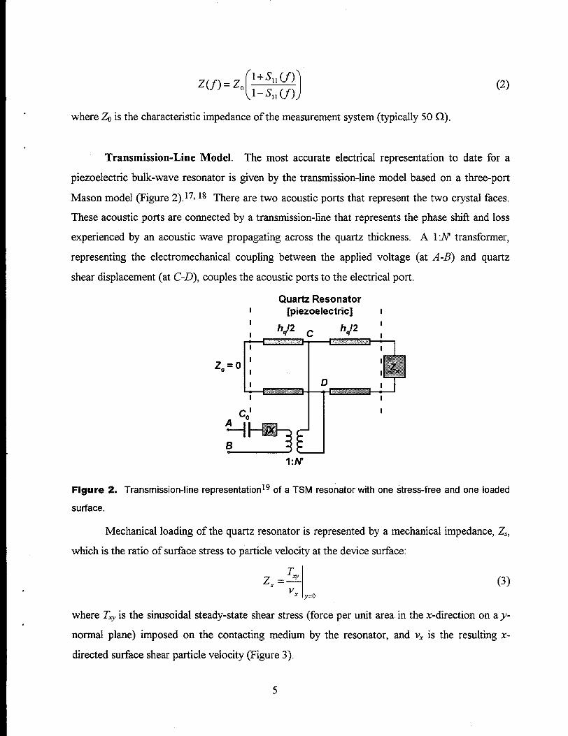
Transmission-Line Model.

piezoelectric bulk-wave resonator is

The most accurate electrical

given by the transmission-line

representation to date for a

model based on a three-port

Mason model (Figure 2). 17>18 There are two acoustic ports that represent the two crystal faces.

These acoustic ports are connected by a transmission-line that represents the phase shifl and loss

experienced by an acoustic wave propagating across the quartz thickness. A 1:N’ transformer,

representing the electromechanical coupling between the applied voltage (at A-B) and quartz

shear displacement (at C-D), couples the acoustic ports to the electrical port.

Quartz ResonatorI [piezoelectric] I1

h#2 ~ hJ2 ‘1 I:.,,,,>,,,,,,,,..,,*;;>y,.>,I 1

Z*=O ‘II D I~..x&*~+lkxx>,.,. :%x.-

~ ~ I

co’ I

‘3F--i

.>..:,,/..,,,:B

l:iv

Figure 2. Transmission-line representation19 of a TSM resonator with one stress-free and one loaded

surface.

Mechanical loading of the quartz resonator is represented by a mechanical impedance, 2$,

which is the ratio of surface stress to particle velocity at the device surface:

z. .L (3)vx y=o

where TV is the sinusoidal steady-state shear stress (force per unit area in the x-direction on a y-

normal plane) imposed on the contacting medium by the resonator, and v. is the resulting x-

directed sutiace shear particle velocity (Figure 3).

5

Y

Figure 3. Cross-sectional view of an unperturbed TSM resonator where T,y is the surface shear stress,

VXis the resulting particle velocity and w is the resulting particle displacement in the x-direction.

For the unperturbed quartz crystal, both of the sutiaces may be considered as stress-free

boundaries (neglecting electrode mass) which gives Z, = O, analogous to a short-circuit at both

acoustic ports. In most sensing applications, one of the ports is unloaded and acts as a short

circuit (2. = O), while the other is terminated by a non-zero surface mechanical impedance, Z,.

The complex electrical input impedance for the quartz resonator described by the transmission-

line model in Figure 2 iss

Z= ZAB=-J- “ ~zcDjdo ‘Jx+(N’)z

(4)

where ZCDis the complex mechanical impedance, m= 2# (f is the excitation frequency), X is the

reactance of the piezoelectric interactio~ N’ is the transformer turn ratio representing the quartz

electromechanical coupling, CO is the static capacitance of the resonator, and j = (-l)%.

Expressions for X and N’ are defined in the literature.20 Further development of transmission-line

components leads tog

[

K’ 2tan(4,/2)- j(.Z./Z,)zAB=~l-—

jdo b, 1- j(z, j-zq)cot(4qd (5)

where K2 is the complex electromechanical coupling factor for lossy quartz (Table 1), @qk the

complex acoustic phase shift across the lossy quartz, and Z~ is the quartz characteristic impedance

(Zq = (p~~)% where ~ is the quartz shear elastic constant (Table l)). The electrical impedance in

eq 5 can be represented as a motional impedance, Z~ (arising from mechanical motion), in parallel

with Co as ‘Y19

(6)

.

The first term in eq 6 represents the motional impedance for the unperturbed resonator (Z~O),

while the second term represents the motional impedance created by the sutiace load (Z~l).

Permittivity, Sq(A2 S4g-l cm-3) 3.982 X 10-13

Viscosity, q~ (g cm-l s-l) 3.5 x 10-3

I Shear elastic constant, ~~ (dyne cm-2) I 2.947 X 1011 II Density, p~ (g cm-3) I 2.651 I

Electro mechanical coupling factor, K2 7.74 x 10-3

Wave velocity, v~(cm S-l) I 3.34 x 105 ITable 1. Properties of AT-cut quartz.21

The Unperturbed Resonator. For an unperturbed resonator operating at frequencies

near the mechanical resonance (~ ~ iVZ), the transmission-line model can be simplified to get an

expression in terms of lumped-elements. By using the identity tan(@~/2) = 4@~/[(lVZ)2- #~2] and

q:= [(~@2 - 8K2]/(1 +.j~ where ~= UqJpq, and assuming that 8K2 <{(iVz)2 and co= ~, the first

term in eq 6 can be approximated as10

“=k[*-ll”R1+’mL]+k(7)

where q~ is the effective viscosity for quartz (Table 1), to. = 2zf~ where js is the series resonant

frequency for the unperturbed TSM resonator, and N is the resonator harmonic number. This

approximation describes the motional impedance for the ButterWorth-Van Dyke (BVD)

equivalent circuit of an unperturbed resonator (Figure 4a with Z~l = O). It has been shown

previously that this simpler lumped-element model can be used instead of the transmission-line

representation, and the deviation between the models is negligible for the unperturbed

resonator. 19

7

(a)1’

(b) T

Figure 4. Modified Buttetworth-Van Dyke equivalent circuit with (a) a complex surface impedance

element,Znl’,and (b) a motional inductance, L2, and resistance, R2.

The BVD model consists of a “static” and “motional” arm in parallel. The static arm consists of a

capacitance, CO*,where

Co”= co+c, (8)

CP is the parasitic or stray capacitance, external to the quartz, due to the geometry of the test

fixture and electrode pattern. The motional arm, containing Ll, Cl and RI, arises due to the

electromechanical coupling of piezoelectric quartz (i.e., due to the motion of the resonating

crystal). The capacitive component, Cl, represents the mechanical elasticity of the system; the

inductive component, Ll, represents inertial mass changes; and the resistive component, RI,

represents dissipation of energy due to viscous effects, internal friction, and damping from the

cxystal mounting. The static capacitance, CO*, dominates the admittance (reciprocal of

impedance) away from resonance, whale the motional contribution dominates near resonance.

The elements of the equivalent circuit for the unperturbed resonator are given by10

SAco =_&

9(9)

c, =SK*CO

(ivZ)’(lo)

L,=~ (11)Cf.fc,

8

R1=~ (12)Pqcl

where Sq is the permittivity for quartz (Table 1), A is the effective electrode area, and hq is the

quartz crystal thickness.

The Surface Loaded Resonator. A load on the surface of a resonator can be represented

by a surface mechanical impedance, Zs (eq 3). This is shown for the transmission-line model in

Figure 2. Similarly, the lumped-element model is modified with a motional impedance, Z~l, as

shown in Figure 4a. Z. is a complex quantity: the real part, Re(Z,), corresponds to the component

of surface stress in phase with the surface particle velocity and represents mechanical power

dissipation at the surface; the imaginary part, Im(Z,), corresponds to the stress component 90°

out-of-phase with particle velocity and represents mechanical energy storage at the surface.

The transmission-line model is the more accurate of the two models since it imposes no

restrictions on the sufiace mechanical load impedance. However, the lumped element approach is

easier to visualize and often requires less effort to extract parameters. It has been shownlg that, in

all cases, the relative deviations in the resonator parameters (Aj and AR) computed by the two

models does not exceed 3°/0 for most practical loading conditions operating at the resonator

fimdamental frequency. Theoretically, if the ratio of Z, to Z~ does not exceed 0.1, the lumped-

element model always predicts responses within 1°/0 of those for the transmission-line model.

Thus the motional impedance created by a surface load (described by the second term in eq 6) can

be approximated by

(13)

Furthermore, Z~l is complex and can be separated into real and imaginary components (see Figure

4b):

Z: = R2 + joL2 (14)

The equivalent circuit parameters, R2 and L2, can be related to Z, by

R2 = ‘zRe(Z, )

4K2(D,C0 Zq(15)

and

X2 = mL2 =NZ Inl(z$ )

4K 2m~Co Zq(16)

Eq 7 can be modified to give the total motional impedance, described by the lumped-element

model, for a surface-loaded resonator:

1Z.=(R1 +R2)+ju(L, +L2)+—

jci)C1(17)

There are three prima~ surface load types that can be applied to a quartz resonator: an

ideal mass layer, a fluid, and a viscoelastic medium. The first two are special cases of the latter.

Addition of these layers to the resonator surface will present different sutiace mechanical

impedances, and hence change the electrical characteristics of the system. This section relates Z.

to the physical parameters of the different surface loads, not only for single-layered, but also for

multi-layered and semi-infinite systems. The different systems studied are summarized in Table 2

at the end of the section. The list is not exhaustive, but the cases presented describe the majority

of single/multi-layered systems likely to be encountered on the TSM resonator.

Ideal Mass Layer. A film that is sufficiently thin and rigid so that there is negligible

acoustic phase shift, ~, across the layer thickness maybe approximated as an ideal mass layer, i.e.,

one that is infinitesimally thin, yet imposes a finite mass per unit area on the resonator surface. In

this case the entire layer moves synchronously with the quartz surface (Figure 5).

Y

Figure 5. Cross-sectional view of a TSM resonator with a layer behaving as an ideal mass layer on the

upper surface. The acoustic phase shift across the layer is negligible.

10

The sufiace stress,

where v.. is the surFace

TV, required to sinusoidally accelerate a mass layer is

Tw = p,tixo (18)

particle velocity and tiXO= dvXO\i3?. p, is the mass per unit area

contributed by the layer (p, = h,piml, where h, and Pinl are the thickness and density of the ideal

mass layer, respectively). For a sinusoidal oscillation

Vx= vWe’@’ (19)

and

TW= j~xop= (20)

The surface mechanical impedance, Z,, associated with an ideal mass layer is obtained by

combining eqs 3 and 20 to give

Z. = jup, (21)

Combining eq 21 with 15 and 16 gives the motional impedance elements arising from the ideal

mass layer:22

R2=0 (22)

and

X2= ‘z =4K2qC0 Zq

(23)

From eqs 22 and 23, it can be seen that there is no power dissipation (Rz), but only energy storage

(X2) arising from the kinetic energy of the mass layer. This energy storage is proportional to the

surface mass density.

The unperturbed series resonant frequency, J, is defined as the frequency at which the

motional reactance is zero, i.e.,

Solving eq 24 for ~, and noting that a, = 2@~, gives

(24)

(25)

For the perturbed resonator with mass loading:

11

(26)

This is equivalent to the Sauerbrey equation (eq 1) when iV=l.

Example. Figure 6 shows an example of the mass loadlng effect on the TSM resonator

electrical characteristics near resonance for a 6 MHz AT-cut quartz resonator. The curves are the

measured response for (a) the unperturbed device and (b) the TSM resonator loaded with 160 run

Si02 layer. The primary effect of the mass layer is to translate the admittance curves towards

lower frequency without affecting the admittance magnitude. This is consistent with eqs 22 and

23 where there is only an inductive component, Lz, added to the electrical equivalent circuit. This

element represents the increased kinetic energy contributed by the mass layer moving

synchronously with the resonator sutiace.

100

10

0.1

0.01

90

60

-60

-90

5.875 5.880 5.885 5.890

f (MHz)

Figure 6. Electrical admittance vs. frequency for a TSM resonator before and after deposition of a 160

nm Si02 layer.

12

Semi-infinite Fluid. When aTSMresonator isoperated in a fluid, theshear motion of

the crystal sufiace viscously entrains fluid close to the resonator sufiace (Figure 7). The velocity

field, VX,generated by this in-plane shear oscillation is determined by solving the Navier-Stokes

equation for one-dimensional plane-parallel flow:zs

d’vx

“7= “+x (27)

where ~ and qz are the liquid density and shear viscosity, respectively. The solution is

‘X~> ~)= VXOe-y~ej@t (28)

Eq 28 represents a damped shear wave radiated into the fluid by the oscillating device surface. y

is the distance from the surface and y is the complex propagation factor for the acoustic wave:

Y= (1y ‘(l+j)

Substituting eq 29 into eq 28 leads to

[ (J-3sin($)le’@tVx(j,t)=vxoe-’~ CCLSZ

where Jis the decay length of the shear wave:

We note that the decay length is related to the kinematic viscosity (ql/P) of the fluid

(29)

(30)

(31)

Figure 7. Cross-sectional view of a TSM resonator with a Newtonian fluid on the upper surface.

13

Newtonian Fluid Case. A Newtonian fluid is one in which the shear stress and the

gradient in fluid velocity are related by a constant, independent of amplitude or fi-equency. The

shear stress imposed by the resonator surface on the liquid to generate the velocity field of eq 30

is

i

&xTv = –ql

0 ,=,(32)

The surface mechanical impedance contributed by a semi-infinite Newtonian fluid is obtained by

combining eqs 3, 30 and 32:

(33)

Combining eqs 15, 16 and 33 gives the motional impedance elements arising from the semi-infinite

Newtonian fluid in contact with one surface of the resonator:

(34)

Newtonian liquid loading leads to an equal component of energy storage (X2) and power

dissipation (R2). The motional reactance, X2, represents the kinetic energy of the entrained liquid

layer and results in a decrease in the frequency of oscillation. The motional resistance, Rz,

represents power radiated into the contacting liquid by the oscillating device surface and results in

resonance damping.

Example. When liquid contacts one face of the TSM resonator, the electrical response

changes, as described by the elements R2 and X2. Figure 8 shows admittance vs. frequency data

(points) measured as the density-viscosity product @ql) of a solution contacting the resonator

varies. With increasing ~ql, the admittance magnitude shows both a translation of the series

resonant peak toward lower frequency and a diminution and broadening of the peak. The solid

lines in Figure 8 are admittances calculated from the equivalent circuit model when best-fit X2 and

& values are included. The model accurately produces the admittance vs. frequency curves

measured under liquid loading using fixed parameters determined from the unloaded resonator.

The translation of the admittance curves arises from the reactance contribution, X2, and the

broadening and diminution of the resonance peaks arises from the resistance contribution R2.

14

3.0

2.5

2.0E

, E- 1.5

~1.0

0.5

0.0

90

60

g 30~

>% 0

-30

-60

4.965 4.970 4.975 4.980

f (MHz)

Figure 8. Electrical admittance vs. frequency near the fundamental resonance with glycerol (in water)

solutions contacting one side of the TSM resonator. Numbers indicate percentage glycerol. The solid

curves are fits to the measured data points.22

Similarly, Figure 9 shows the equivalent circuit parameters, RZ and Xz, as a fl.umtion of

@ql~ obtained for various glycerol/water solutions. It can be seen that the plot is linear and Rz =

Xz, as predicted by eq 34. The best fit from the measured response is extremely close to the

, predicted response.

15

3.0

2.5

2.0

1.5

1.0

0.5

0.0---0.0 0.2

Figure 9. Equivalent circuit parameters

which exhibit Newtonian characteristics.

Maxwellian Fluid Case. A

0.4 0.6 0.8

(PF71)”2(9 cm-z S-”2)

(R2 and X2) as a function of (pql)ln for glycerol/water solutions

Maxwell fluid is one type of non-Newtonian fluid that

considers the finite reorientation time of molecules under shear stress. The fluid exhibits a first-

order relaxation process:zg

q(a))= ~;I+ Ju’r

(35)

where q. is the low frequency shear viscosity and r is the relaxation time (r= qo/G~ where G~ is

the high frequency rigidity modulus). When the strain rate is low, a<< 1, and the Maxwell fluid

behaves as a Newtonian fluid. However, when ur = 1, unhke Newtonian fluids, the elastic energy

cannot be totally dissipated in viscous flow and some is stored elastically. (Also it is interesting to

note that when aw>>1,juq = Go and the fluid behaves much like a solid.)

Eq 35 can be substituted into eq 32 to give an expression for the shear stress. Then, in a

fashion similar to that used for the Newtonian fluid, eqs 35 and 29 are combined to give an

expression for the complex propagation factor:

jwz(1+j*)Y2=—Vo

(36)

Eqs 32 and 3 then give an expression for the surface mechanical impedance for a Maxwell fluid:

16

(1z

~ = -iwl~os

(37).l+jwr

Combining eqs 15, 16 and 37 gives the motional impedance elements arising from the semi-infinite

Maxwell fluid:

Rz = ‘“ [f#[l+J*-4K2#,cozq

and

(39)

These statements agree with derivations by Mason in 1965.25

It can be seen that when a <{ 1, eqs 38 and 39 reduce to those of a semi-infinite

Newtonian fluid (eq 34). When u is not negligible, Rz > X2.

Example. Figure 10 shows the motional impedance parameters computed for fluids with

different viscosities showing the influence of molecular reorientation time.

r \\ aE I I 1 \ \]

0.01 0.1 1 10 100

Viscosity, q.(P)

Figure 10. Computed motionai impedance parameters (/?2, XJ for Newtonian and Maxwell fluids as a

function of static viscosity and high frequency rigidity modulus: G== (a) 3 x 107, (b) 1 x 108and, (c)3x

108dyne cm-2.

17

At low viscosity (qo ~ 0.1 P), the fluid response is characteristic

However, as ~0 increases, the response deviates from Newtonian

X2, and X2 eventually decreasing with increasing qo.

of a Newtonian fluid (R2 = X2).

behavior, characterized by Rz ~

For many materials the relaxation time, ~, and the low frequency viscosity, qo, area strong

fi.mction of temperature. This influences their theological properties. Figure 11 shows the

motional resistance, Rz, and reactance, X2, measured for a TSM resonator immersed in two

different synthetic lubricants. At high temperature, when m<{ 1, R2 s X2, and both lubricants

behave as Newtonian fluids. At low temperature, Rz > X2 and the lubricants exhibit Maxwell fluid

characteristics. The lubricant containing the polymeric additive used as a viscosity enhancer

shows significantly more non-New-tonian behavior than the base stock.

\ ~ R2 - oil base stock I

❑m:.:.

“n.“.

n. .

R2 B X2 R==X2Maxwellian Newtonian

Fluid Fluid1

-30 0 30 60

T (“C)

Figure 11. Experimental motional impedance parameters (Rz, X2) for two synthetic lubricants as a

function of temperature.24

Viscoelastic Layer: Finite Thickness Case. A finite viscoelastic layer is one with a film

thickness smaller than several decay lengths so that the shear acoustic wave generated at the

resonator/film interface is reflected at the film/air interface (Figure 12). Therefore, the surface

mechanical impedance is dependent upon the phase shift and attenuation of the wave propagating

18

across the film, i.e., it depends upon the nature of the intefierence between the waves generated at

the lower film surface and those reflected from the upper (film/air) sutiace.

(c)

,... ,.,:.-..

Figure 12. The dynamic film response generated by the oscillating resonator surface varies with the

acoustic phase shift, #, across the film: (a) for ++<<z/2, synchronous motion occurs; (b) for # s n/2,

overshoot of the upper film surface in-phase with the resonator surface occurs (film resonance occurs

when # = nf2); (c) for q$> 7d2, the upper film surface is 180° out-of-phase. The film is the thin region at

the top; the crystal is below. The magnitude of shear displacement in the quartz and the film are scaled

to illustrate the differing effects.

Shear displacement in a viscoelastic layer can be described by the equation of motionlT

(40)

where G is the complex shear modulus (G = G +jG”, where G is the storage modulus and G is

the loss modulus) and ~is the film density. This equation can be solved to give the displacement,

UX,in the film as a fimction of distance from the resonator surface and time. The solution is a

superposition of waves propagating in opposite directions due to reflection at the film/air

intefiace:

19

‘.6’> ~)=(Ae-yy + &yy )-ejot (41)

where A and 1? are constants and y is the complex wave propagation constant (determined by

substituting eq 41 into eq 40):

(42)

Two boundary conditions are applied to solve for xl and Bin eq 41:

(1) ZJX(0)= UXOi.e., continuity of particle displacement at the resonator/film intetiace; and

(2) TV(kf )= o i.e., the upper film surface is stress free.

ly is the film thickness. After solving for A and B, eq 41 can be written as

[ 1%(W)=%‘y(h:;:;:-y)e’d (43)

By substituting expressions for VXand TV into eq 3, an expression for the sutiace mechanical

impedance seen at the resonator/film interface is obtained: 11

(44)Z= = (Gpf)x tanh(y~f)

The hyperbolic tangent of the complex argument, yhfi in eq 44 makes it diflicult to separate the

load impedance, Z~l, into its real and imaginary components, R2 and X2, except in a few limiting

cases. Thus, it is customary to treat the finite viscoelastic layer as having a single lumped-element

complex electrical impedance.

When the phase shift, ~ [$ = Re(@f)], across the film is small, the film’s upper surface

moves synchronously with the resonator surface (Figure 12a). Since the shear displacement is

uniform across the film, no elastic energy is stored or dksipated due to inertial effects. In this

regime, the device response is insensitive to G, and only dependent upon the layer mass, p, as

described previously. When the phase shift across the film becomes appreciable, the upper film

sutiace lags behind the driven resonator/film intetiace (Figure 12b). Significant elastic energy is

stored and dissipated. In this case, the resonant frequency and damping depend upon film

thickness, density, and shear elastic properties.

When ~= z/2, i.e., the film thickness is one-quarter of the shear wavelength, a resonance

effect is created within the film causing maximum coupling of acoustic energy from the TSM

resonator to the film. At this point, the interaction between the resonator and film exhibits

20

characteristics of coupled resonators. 11 Dramatic changes in the motional impedance occur at =

film resonance due to the enhanced coupling ofacoustic energy into theillm. Film resonance

effects have been recently demonstrated during the electrodeposition of polymer films by varying

hfz6j 27 Film resonance can also be achieved by varying G or ~ (e.g., as they change with

temperature).s~ 11 As & surpasses z/2, the upper and lower surfaces go from an in-phase to an

out-of-phase condhion (Figure 12c).

Example. The change in film dynamics with ~ has a profound effect on device response

as exemplified by Figure 13. This shows the admittance magnitude data vs. frequency for a 3 pm

trans-polyisoprene film on a 5 MHz TSM resonator operating in the third harmonic as a finction

of temperature. The shear modulus, G, of the film is altered by varying the temperature, thus

allowing &to go through z42 and exhibit film resonance. Film resonance is indicated by a jump in

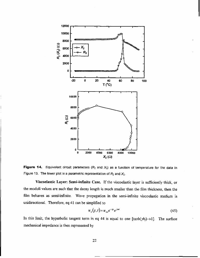
the admittance peak to higher frequency. Figure 14 shows the corresponding parametric plot (R2

vs. X2) for the data of Figure 13 fitted to the lumped element equivalent circuit of Figure 4.

Resonance is observed when the conductance reaches a minimum (resonant resistance, &,

reaches a maximum).

Figure 43. Admittance magnitude vs. frequency as a function of temperature

polyisoprenefilm on a 5 MHz AT-cut TSM resonator operating in the third harmonic.

21

for a 3 pm trans-

10000

8000

2000

0

11 1 I I I I I-20 0 20 40 60 80 100

T (“C)

10000

8000

~ 6000

z“

4000 -

2000 -

0 I Io 2000 4000 6000 8000 10000

x*(!2)

Figure 14. Equivalent circuit parameters (f?z and X2) as a function of temperature for the data in

Figure 13. The lower plot is a parametric representation of R2 and X2.

Viscoelastic Layer: Semi-infinite Case. If the viscoelastic layer is sufficiently thick, or

the moduli values are such that the decay length is much smaller than the film thickness, then the

film behaves as serni~infinite. Wave propagation in the semi-infinite viscoelastic medium is

unidirectional. Therefore, eq 41 can be simplified to

‘X~~t)=uXOe-wej& (45)

In this limit, the hyperbolic tangent term in eq 44 is equal to one [tanh(@J+l]. The surface

mechanical impedance is then represented by

22

Z. = (Gpf )x

By combining eqs 15, 16 and 46, the equivalent circuit elements can be obtained:

(46)

R, = ‘n

I

pf (IGI+ G’)”

4K2qCoZq 2

and

L, = ‘n

I

pf (IGI- G’)

4K 20:CoZq 2

(47)

where IGI = [(G’ )2 + (G’’)2]ln. It is possible to invert eqs 47 and 48 so that film storage and loss

moduli can be extracted directly from experimentally determined values ofllz and L*.

Example. Figure 15 shows the theoretical response for a 10 MHz resonator using the

lumped-element model of Figure 4 for a viscoelastic layer where G’ = G“ = 107 dyne cm-2 and ~=

1 g cm-3. It can be seen that for thicknesses above 4 pm,

parameters (R2 and X2)are not dependent upon hfi i.e., the film is

TSM resonator is not “seeing” anything beyond this thickness.

reflection at the fihn/air interface.

the electrical equivalent circuit

behaving as semi-infinite and the

In this case there would be no

3000 ] , I I I I 1

2500

2000

1500

1000

500

0

n El:R2—— X2

/II/1II

-1!II

-/ \ ~-.–––––––––––––:/ ,,/

+finite limit

1’ I I I 1 10 2 4 6 8

hf (~)

Figure 15. Theoretical equivalent circuit parameters (R2 and X2)

viscoelastic layer where G = G“ = 107 dyne cm”2 and ~ = 1 g cm-3. The

/?f>4,&Tn.

10

versus film thickness for a

film becomes semi-infinite for

23

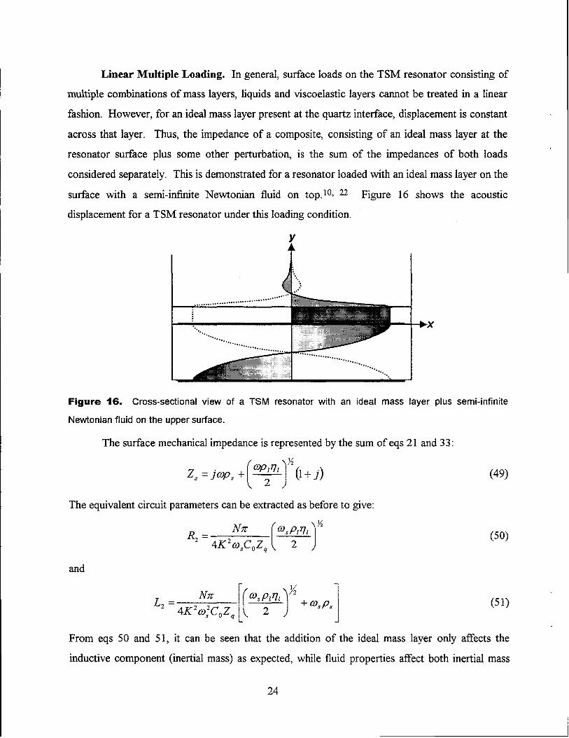
Linear Multiple Loading. In general, surface loads on the TSM resonator consisting of

multiple combinations of mass layers, liquids and viscoelastic layers cannot be treated in a linear

fashion. However, for an ideal mass layer present at the quartz intetiace, displacement is constant

across that layer. Thus, the impedance of a composite, consisting of an ideal mass layer at the

resonator surface plus some other perturbation, is the sum of the impedances of both loads

considered separately. This is demonstrated for a resonator loaded with an ideal mass layer on the

surface with a semi-infinite Newtonian fluid on top. 1°’ 22 Figure 16 shows the acoustic

displacement for a TSM resonator under this loading condition.

I

+x

Figure 16. Cross-sectional view of a TSM resonator with an ideal mass layer plus semi-infinite

Newtonian fluid on the upper surface.

The surface mechanical impedance is represented by the sum of eqs 21 and 33:

The equivalent circuit parameters can be extracted as before to give:

iV?r

(1

zR, = @sPI71

4K2m~COZq 2

and

‘2=,K&~ozq[(os;1q1~+oS~S]

From eqs 50 and 51, it can be seen that the addition

inductive component (inertial mass) as expected, while

(49)

(50)

(51)

of the ideal mass layer only affects the

fluid properties affect both inertial mass

24

and viscous darnping equally, as before. Z~l is dependent upon the surface mass density, p., of

the ideal mass layer and the density, p, and viscosity, VI,of the liquid. Similarly, solutions can be

obtained for resonators loaded with an ideal mass layer plus Maxwell fluid or viscoelastic material

(finite or semi-infinite). For simplicity, these solutions are summarized in Table 2.

Example. Figure 17 shows the theoretical responses using the lumped-element model of

Figure 4 for a 10 MHz device for (a) an unperturbed resonator, (b) fluid loading only, and (c) an

ideal mass layer plus fluid loading. As shown previously, the effect of adding a fluid onto the

resonator sufiace is to decrease the frequency and increase the damping of the spectrum. In

additio~ the ideal mass layer translates the spectrum towards lower fi-equency without damping

the resonator response. It is possible to separate the physical properties of the two layers due to

the linear relationship between the energy storage and power dissipation for a Newtonian fluid.

Any excess storage can be attributed to the ideal mass layer.

1e-2~ 1 I 1 , 1

; 1e-2

z~

u~

$ le-3 : te.3 ~sr

:

En

~5

1e..i~

1e-4

1e-51 I I 1 I

90

60

~

230

mgo~~n -30>

-60

-90 a

1 1 1 1 1

‘ 9.98 9.99 10.00 10.01 10.02

f (MHz)

Figure 17. Theoretical admittance response (magnitude and phase) using the lumped-element model

of Figure 4 for a 10 MHz TSM resonatofi (a) an unperturbed

mass layer plus fluid loading. P = 1 g cm-3 and VI= 1 cP.

resonator, (b) fluid loading only (c) an ideal

25

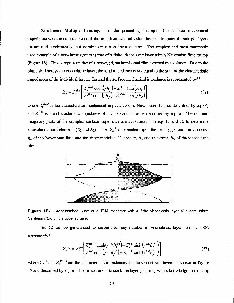
Non-liiear Multiple Loading. In the preceding example, the surface mechanical

impedance was the sum of the contributions from the individual layers. In general, multiple layers

do not add algebraically, but combine in a non-linear fashion. The simplest and most commonly

used example of a non-linear system is that of a finite viscoelastic layer with a Newtonian fluid on top

(Figure 18). This is representative of a non-rigid, surface-bound film exposed to a solution. Due to the

phase shifi across the viscoelastic layer, the total impedance is not equal to the sum of the characteristic

impedances of the individual layers. Instead the surface mechanical impedance is represented byla

z=. Zf”[

6’Z~ cosh hf )+ Z~ sinh (yhf )

Z? cosh(yhf )+ Z~ sinh (yhf J1(52)

where ZY~ is the characteristic mechanical impedance of a Newtonian fluid as described by eq 33;

and Z$lm is the characteristic impedance of a viscoelastic film as described by eq 46. The real and

imagirwy parts of the complex surface impedance are substituted into eqs 15 and 16 to determine

equivalent circuit elements (llz and X2). Then Z~l is dependent upon the density, p, and the viscosity,

ql, of the Newtonian fluid and the shear modulus, G, density, ~, and thickness, ?zfiof the viscoelastic

film.

Figure 18. Cross-sectional view of a TSM resonator with a finite viscoelastic layer plus semi-infinite

Newtonian fluid on the upper surface.

Eq 52 can be generalized to account for any number of viscoelastic layers on the TSM

resonators> 14

(53)

where ZC‘“)and ZY1) are the characteristic impedances for the viscoelastic layers as shown in Figure

19 and described by eq 46. The procedure is to stack the layers, starting with a knowledge that the top

26

(outermost) of the composite resonator is stress free (or in contact with a semi-infinite fluid), and work

towards crdculating the surface mechanical impedance at the resonator/film intenface. This makes it

possible to study the effects of many viscoelastic layers on the surface of the TSM resonator, although

characterizing or extracting the density, thickness, and shear moduli of the individual layers would be

@ = o k Figure 19,difficult due to the increasing number of parameters. It should be noted that if Z.

i.e., there is only one viscoelastic layer present, then eq 53 will reduce to eq 44 for a finite viscoelastic

layer (Zc(~+1)= Zcm = 0)

characteristic impedanceIgg

impedance of interface

f)+l Z=n+l Zcn+l

J z~n+l

1 I I

z~3 ‘

I

2 ZC2+ z~2

1

1 Zcl

.....--..........

~ Surface stress, Tv

0

Figure 49. Model for calculating tie mechanical impedance imposed on a TSM resonator by multiple

viscoeiastic layers.

The surface mechanical impedance model given by eq 53 and illustrated in Figure 19 also can

be used to represent viscoelastic films with non-homogeneous moduli or density. Such could exist for

a polymer film in which a solvent diffises slowly into the bulk over time; the outer portion of the film is

more plastic than polymer near the resonator. In this case, the polymer film can be divided into several

segments, each with a graded modulus and density. An effective swface mechanical impedance is then

computed. Any layered system of viscoelastic films

layers) can be treated with this non-linear model.

27

and fluids (or a system with interspersed mass

Combhations of Lkear and Non-1inear Loadings. Figure 20 shows the shear

displacement of a TSM resonator loaded with three different layers: an ideal mass layer next to the .

resonator, a viscoelastic layer, and a semi-infinite Newtonian liquid on top. The surface mechanical

impedance for this system is simply eq 52 for the viscoelastic layer with liquid overlayer plus the .

contribution from the ideal mass layer (eq 21). The final expression for Zs can be extracted from the

last entry in Table 2 using n = 1 and Zyl) from eq 33 for a Newtonian liquid. Note here that values of

n are assigned only to the layers that contribute to the non-linear loading, and the mass layer is treated

separately. Having an expression for 2s, eqs 15 and 16 are again used to describe the electrical

components for the equivalent circuit representation. Znl is dependent upon the surface mass density,

PS, of the ideal mass laye~ the shear modulus, G, density, ~, and thickness, hfi of the viscoelastic film;

and the density, P1, and viscosity, VI,of the Newtonian fluid.

$

Figure 20. Cross-sectional view of a QCM with an ideal mass layer plus finite viscoelastic layer plus semi-

infinite Newtonian fluid on the upper surface.

Example. For this example, we choose to look at the electrochemical deposition of poly(2,2’-

bithiophene) (PBT) conducting polymer films onto 10 MHz AT-cut quartz resonators with gold

electrodes. This system has been previously studied7 and by a stepwise process shear moduli values

for the polymer film were extracted. The ideal mass layer accounts for any trapped material in stiace

roughness features (entrapped material moves synchronously with the resonator surface and so can be

treated as an ideal mass layer); the fluid represents the deposition solution; and the viscoelastic layer

represents the polymer film. The solution used was 5 mmol drn-3 bithiophene, 0.1 mol din-3

tetraethylammonium tetra.fluoroborate in acetonitrile and the deposition potential, E, was 1.125 V.

28

Figure 21 shows the crystal impedance spectra acquired dynamically during the course of the

deposition process. Upon application of the potential step @ = Oto 1.125 V), the resonance moves to

lower iiequency and the peak admittance decreases. This is consistent with the deposition of a film in

which there is substantial energy loss, i.e., a viscoelastic PBT film.

I t I I I

uncoated crysta

r1.125 V 3 reins - in solution

3

Ov-1 ,minsdll

16 mins~

24 min+

#)32 reins!

40 reins

9.915 9.920 9.925 9.930 9.935 9.940

f (MHz)

Figure 21. Crystal impedance spectra acquired during the electrodeposition of poly(2,2-bithiophene).

Solution 5 mmol din-3 bithiophene, 0.1 mol din-3 tetraethylammonium tetrafiuoroborate, acetonitrde. E =

1.125 V. Numbers indicate time (rein) from application of potential step.7

This complex three-layer model is of significant value if the parameters of interest (in this case

the shear modulus of the film) can be extracted. As can be seen from Table 2, there are many

parameters that need to be predetermined in this model in order to extract unique values for the film

shear modulus. This can be accomplished in a stepwise manner. First, the deposition solution is

characterized so that Plql and p~ are determined as indicated previously for an ideal mass layer in

contact with a Newtonian fluid. The values obtained were plql = 0.00289 g2 cm~ S-l (theoretical =

0.00283 g2 cm_”S-1)28and p. = 1.03 ~g cm-2. Assuming a density of 1 g cm-3, this corresponds to an

effective roughness thickness of 10.3 nm. Taking ~ = 1 g cm-3 and calculating hf from the charge

29

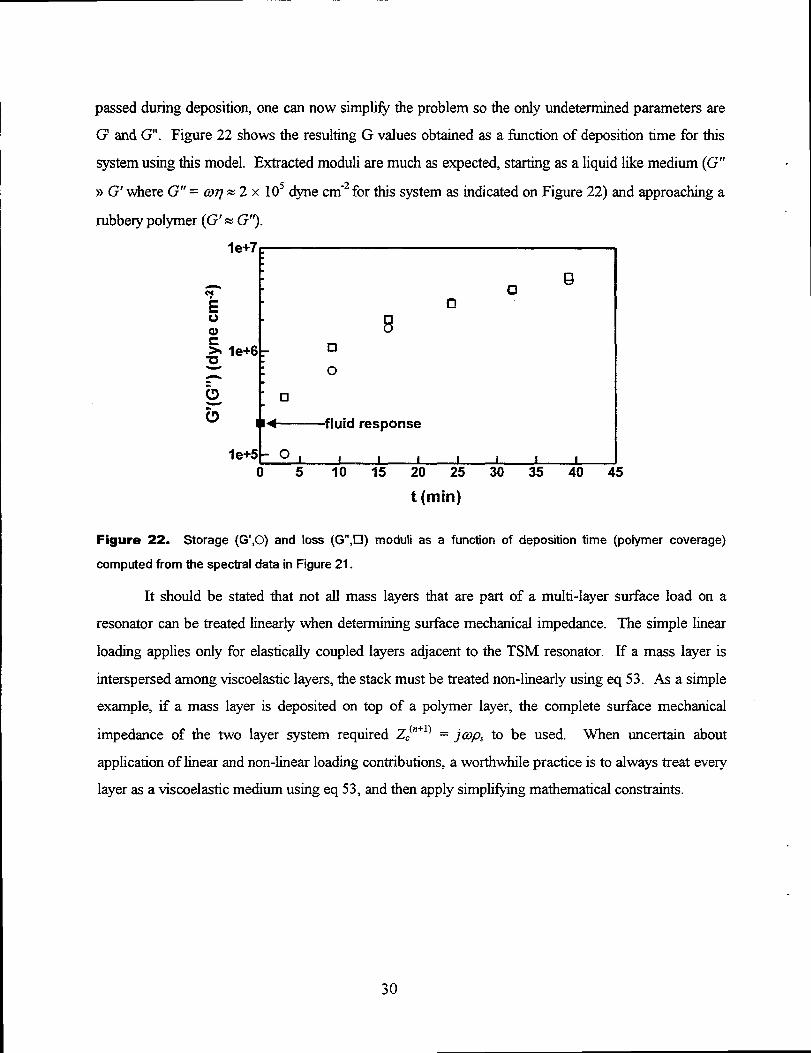
passed during deposition, one can now simplifj the problem so the only undetermined parameters are

G’ and G“. Figure 22 shows the resulting G values obtained as a fiction of deposition time for this

system using this model. Extracted moduli are much as expected, starting as a liquid like medium (G”

})G’ where G“ = tvq N 2 x 105 dyne cm”2for this system as indicated on Figure 22) and approaching a

rubbery polymer (G’= G“).

‘e+7~k

o

8

response

I I 1 1 I 1 iO 5 10 15 20 25 30 35 40 4

t (rein)

Figure 22. Storage (G,O) and loss (G,U) moduli as a function of deposition time (polymer coverage)

computed from the spectral data in Figure 21.

It should be stated that not all mass layers that are part of a multi-layer surface load on a

resonator can be treated linearly when determining surface mechanical impedance. The simple linear

loading applies only for elastically coupled layers adjacent to the TSM resonator. If a mass layer is

interspersed among viscoelastic layers, the stack must be treated non-linearly using eq 53. As a simple

example, if a mass layer is deposited on top of a polymer layer, the complete surface mechanical

impedance of the two Iayer system required ZC(n+l)= jap$ to be used. When uncertain about

application of linear and non-linear loading contributions, a worthwhile practice is to always treat eve~

layer as a viscoekistic medium using eq 53, and then apply simpli@ing mathematical constraints.

30

.

The models we have described offer several aspects of sophistication over and above those

previously available. First, they allow one to combine multiple loading elements. This is a

necessity for describing any in situ electrochemical experiment, biosensor syste~ or multi-phase

fluid/deposition monitor. Second, it allows smooth transition between finite and semi-infinite

iilms when. characterizing a system. This is frequently encountered during a deposition

experiment at fixed conditions as the film thickness increases, or during a temperature ramp

experiment at fixed film thickness. Third, the expressions for surface mechanical impedance

readily lend themselves to diagnostic use. For example, one can explore resonator responses

while varying such parameters as film thickness or surface finish, respectively, to distinguish finite

vs. semi-infinite behavior, or “surface entrapped” vs. bulk liquid behavior. Fourth, the model

provides a relatively transparent link between experimental observations (resonator electrical

response) and usefi.d physical parameters intrinsic to the materials used, notably shear moduli and

liquid viscosity. This allows study of direct chemical interactions as they relate to mechanical or

acoustic characteristics.

We recognize there are certain features and situations that are not covered by the

description we offer. First, we have not discussed the case of non-homogeneous layers that are,

in one way or another, composites of some sort, e.g., the case of microscopically porous

materials permeated by fluids of (necessarily) very different theological characteristics. Second,

we have not considered in detail the case of spatially inhomogeneous films, whether in terms of

structure, density, or viscoelasticity. Thkd, we have not explicitly described film resonance

effects, which have been observed in several polymer systems. g>26>27 Nevertheless, we believe

that the generality and simplicity of the model, coupled with the relatively simple diagnostic

characteristics associated with the various cases, make it applicable to a wide variety of systems

and circumstances encountered in interracial studies. Further, we envisage subsequent extension,

as guided by experiment, to incorporate these more complex situations.

31

CONCLUSIONS

We have developed an equivalent circuit model describing the surface mechanical

impedance of several TSM resonator loads. These include rigidly coupled films and non-rigidly

coupled loadings of finite or semi-infinite extent. Important examples of non-rigid loadings

include Newtonian or Maxwell fluids and viscoelastic solids, of which polymers are a very

important class. The model is capable of converting measured electrical impedance data through

surface mechanical impedance to materials properties, such as viscosity, density, and shear

modulus. In the case of finite loading elements, film thickness may also be determined.

The model is extended to a range of multi-element loadings, which may be linear or non-

linear dependent upon the materials involved and location of layers. Specifically, we develop

expressions for two-layer loadlngs, such as a rigid film with a liquid overlayer and a finite

viscoelastic film with liquid overiayer, and for three-layer loadings, such as a rigid layer with a

finite viscoelastic overlayer and a liquid above that. However, we also demonstrate the general

procedure for resonator loading with an arbitray number of theologically distinct overlayers.

For the cases explored, we provide many experimental examples from diverse intetiacial

structures and processes involving a wide range of materials. The success of the model in

handling these physically diverse cases suggests its general utility.

ACKNOWLEDGEMENTS

The authors thank Kent Pfeifer for his carefhl review of the paper. HLB thanks the

University of Leicester, UK for a University Research Studentship. Sandia is a multiprogram

laboratory operated by Sandla Corporation, a Lockheed Martin Company, for the United States

Department of Energy under Contract DE-AC04-94AL85000.

32

.

.

.

Surface Physical Example Surface Mechanical Impedance (Z,) VariablePerturbation Parameters

unperturbed air o

ideal mass layer Sol-gel film j~~. p,

semi-infinite water

[)

z@..Ivl~ (l+j)

p, VINewtonian fluid

semi-infinite High viscosity

[)

xj~~170 i?> 70>~

Maxwell fluid liquidsI+jam

semi-infinite thick polymer film(@fY G’, G“, ~

viscoelastic layer

finite viscoelastic thin polymer film(%Y@@%) G’, G“, ~, ~

film

ideal mass layer + electrochemical

[)jap$ + y ‘(l+j)

F%,p, v

semi-infinite deposition of AgNewtonian fluid

ideal mass layer + oil on an unpolished

[1

%j~~170 % p, 70>~

semi-infinite surface jap, +

Maxwell fluidl+jcor

ideal mass layer + thick polymer film()j~~, + GPf

% p., G’, G“, Fsemi-infinite on an unpolished

viscoelastic layer surface

ideal mass layer + thin polymer filmj~~. +(GPf~tanh@f) ps>G’, G“>

finite viscoelastic on an unpolished ~, h..layer surface

Multiple electrochemical

[

~(n) z (fJ+l)coshk(”)~:))+z!)s~k(n)~:)) G’ G“a

viscoelastic layers deposition of a thin c 2;.) ~~~ (“)~:) + .&+ Sfi (“)/ly)kd

hh ~, qlpolymer film

c

ideal mass layer + electrochemical

[ hi

Z(fl+l)~O&@@+ z(m)~fi$tfl)h~)) ~,, G’, G“cmultiple deposition of a thm ‘op’ +‘$) @ ~O~h (n)~~)+ 2(.:1)~fi (.)htfl)c f R, hfi D, il

viscoelastic layers polymer film on anunpolished surface

Table 2. Summary of surface mechanical impedance (ZJ for various loading conditions on the TSM

resonator

33

A

A, B

c: cl; co; Cp;CO*

“fjl;$

G: G’; G“; GA G(n)

h: hq;h~ hs; h~~

j

K2

L: Ll; Lz

Am

iv

N,

R: RI; R2

S1l

t

Tw

Ux:Uxo

v: Vq;Vx;v~.

x

X2Y

NOMENCLATURE

effective electrode area (cm*)

constants

capacitance (F): motional contribution from unperturbed resonatoq static;

parasitic; sum of static and parasitic

fi-equency (Hz): unperturbed fimdamental; series resonant

shear modulus (dyne cm-2): storage; loss; high frequency rigidity modulus;

shear modulus of nti layer

thickness (cm): quartz; film; ideal mass layeq nfi layer

J-1

electromechanical coupling coefficient

motional inductance (H): unperturbed resonator; surface perturbation

areal mass density (g cm-2)

harmonic number

transformer turn ratio representing the quartz electromechanical coupling

motional resistance (fl): unperturbed resonator; sutiace perturbation

reflection scattering parameter

time (s)

sinusoidal steady-state shear stress in the x-dh-ection on ay-normal plane

(Nm-2)

x-component of displacement (cm): at y=O

velocity (m s-l): acoustic velocity in quartz; x-directed shear particle

velocity; x-directed shear particle velocity at ~0

reactance of the quartz piezoelectric interaction (!2)

surface load reactance (Cl)

admittance (S)

2 ZO;Z~; Z~~; ZCD;Z,; impedance (Q): characteristic impedance of measurement system (typically

50 Q); quartz characteristic impedance; complex electrical input

impedance; complex mechanical impedance; sufiace mechanical impedance

Zm:Zmo;zml motional impedance (S2): unperturbed resonator; surface perturbation

34

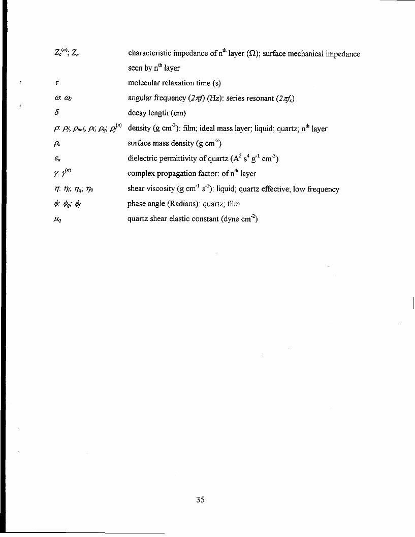
Zy;Zn

j%

&q

P9

characteristic impedance of nti layer (Q); surface mechanical impedance

seen by nfi layer

molecular relaxation time (s)

angular frequency (2x59 (Hz): series resonant (2z$)

decay length (cm)

density (g cm-3): film; ideal mass layer; liquid; quartz; nti layer

surface mass density (g cm-2)

dielectric permittivity of quartz (A2 S4g-l cm-3)

complex propagation factor: of nti layer

shear viscosity (g cm-l S-l): liquid; quartz effective; low frequency

phase angle (Radians): quartz; film

quartz shear elastic constant (dyne cm-2)

35

REFERENCESII

(1)I

~

(2)

I (3)

~(4)

I

I

(5)

(6)

(7)

(8)

(9)

(lo)

(11)

(12)

(13)

(14)

(15)

(16)

(17)

(18)

(19)

(20)

Interactions of Acoustic Wines with I’hin Films and Interfaces, The Royal Society of

Chemistry, London, Faraday Discuss. 1997,107 .

Sauerbrey, G. Z. Phys. 1959,155,206-222.

Nomur&T.; Minemura, A. Nippon Kagaku Kaishi 1980, 1261.

Kanazawa, K, K.; Melroy, O. R. IBMJ Research andDevelopment 1993,37, 157-171.

Buttry, D. A. In Electroanalyticai Chemisby, Ed Bard, A. J, Marcel Dekker: New York,

1991; vol. 17, pp. 1-85.

Oyama, N.; Ohsaka, T. Prog. Polymer Sci. 1995,20,761-818.

Bandey, H. L.; Hillman, A. R.; Brown, M. J.; Marti~ S. J. Farad@ Discuss. 1997, 107,

105-121.

Lucklum, R.; Behling, C.; Cemosek, R. W.; Martin, S. J. J l%ys. D-Appl. Phys. 1997,30,

346-356.

Lucklum, R.; Hauptmann, P. Farad@ Discuss. 1997,107, 123-140.

Mar&in, S. J.; Gransta& V. E.; Frye, G. C. Anal. C’hem. 1991,63, 2272-2281,

Martin, S. J,; Frye, G. C. UltraSon. SjmIp. 1991,393-398.

Martin, S. J,; Wessendofi, K. O.; Gebert, C. T.; Frye, G. C.; Cemosek, R. W.; Casaus, L.;

Mitchell, M. A. IEEE Freq. Cont. Symp. Salt Lake City, UT, USA. 1993, 603-608

Martin, S, J.; Frye, G. C.; Wessendofi, K. O. Sens. Actuators A 1994,44,209-218.

Gransta@ V. E.; Martin, S. J. J. Appl. Phys. 1994, 7.5, 1319-1329.

Martin, S. J.; Frye, G. C.; Sentuna, S. D. Anal. Chem. 1994,66,2201-2219.

Bandey, H. L.; Gonsalves, M.; HNman, A. R.; Glidle, A.; Bruckenstein, S. J. Electroanal.

Chem. 1996,410,219-227.

Rosenbau~ J. F. Bulk Acoustic Wave Theory and Devices; Artech House: Bosto~ 198S.

Christopoulos, C. I%e Transmission-Line Modeling Metho~ Otiord: University

Press,1995.

Cemosek, R. W.; Martin, S. J.; Hlllman, A. R.; Bandey, H. L. IEEE Trans. Ultrasonics,

Ferroelectrics andFreq. Cont. 1998,45, 1399-1407.

Krimholz, R.; Leedom, D. A.; Mathaei, G. L. Electrochem. Lett. 1970,6, 137-44.

36

I

(21) Ballato, A,; Bertoni, H. L.; Tamir, T. IEEE Trans. Microwave Theory Tech. 1974, MTT-

22, 14-25.

. (22) Martin, S. J.; Frye, G. C.; Ricco, A. J.; Senturia, S. D. Anal. Chem. 1993,65,2910-2922.

(23) White, F. M. Viscous FluidFlow; New York: McGraw Hill, 1991.~.

(24) Marti% S. J.; Cernosek, R. W.; Spates, J. J. Digest 8th Int’1. Con$ on Solid-State Sens.

andAct. and Eurosens. IX, Stockholm, Sweden 1995, 712-715.

(25) Mason, W.P. Physical Acoustics, Volume II-Part A; New York: Academic Press, 1965.

(26) Saraswathi, R.; Hillman, A. R.; Martin, S. J. L Electroana2. Chem. in press.

(27) Hillma~ A.R.; Brown M.J.; Martin, S.J. J An. Chem. Sot., in press.

(28) Z-heHandbook of Chemistry and Physics, 75th cd.; C.R.C. Press: Florida, 1994.

.

e

37