assessment of evapotranspiration and soil moisture content ... · pdf fileassessment of...
TRANSCRIPT
Sensors 2008, 8, 70-117
sensors ISSN 1424-8220 © 2008 by MDPI
www.mdpi.org/sensors
Review
Assessment of Evapotranspiration and Soil Moisture Content Across Different Scales of Observation
Willem W. Verstraeten 1,*, Frank Veroustraete 2 and Jan Feyen 3
1 Geomatics Engineering, Katholieke Universiteit Leuven (K.U.Leuven), Celestijnenlaan 200E, BE-
3001 Heverlee, Flanders. E-mail: [email protected].
2 Centre for Remote Sensing and Earth Observation Processes, Flemish Institute for Technological
Research (VITO), Boeretang 200, BE-2400 Mol, Flanders. E-mail: [email protected].
3 Division Soil and Water Management, Katholieke Universiteit Leuven (K.U.Leuven),
Celestijnenlaan 200E, BE-3001 Heverlee, Flanders. E-mail: [email protected].
* Author to whom correspondence should be addressed.
Received: 1 October 2007 / Accepted: 7 January 2008 / Published: 9 January 2008
Abstract: The proper assessment of evapotranspiration and soil moisture content are
fundamental in food security research, land management, pollution detection, nutrient flows,
(wild-) fire detection, (desert) locust, carbon balance as well as hydrological modelling; etc.
This paper takes an extensive, though not exhaustive sample of international scientific
literature to discuss different approaches to estimate land surface and ecosystem related
evapotranspiration and soil moisture content. This review presents:
(i) a summary of the generally accepted cohesion theory of plant water uptake and
transport including a shortlist of meteorological and plant factors influencing plant
transpiration;
(ii) a summary on evapotranspiration assessment at different scales of observation (sap-
flow, porometer, lysimeter, field and catchment water balance, Bowen ratio,
scintillometer, eddy correlation, Penman-Monteith and related approaches);
(iii) a summary on data assimilation schemes conceived to estimate evapotranspiration
using optical and thermal remote sensing; and
(iv) for soil moisture content, a summary on soil moisture retrieval techniques at
different spatial and temporal scales is presented.
Sensors 2008, 8
71
Concluding remarks on the best available approaches to assess evapotranspiration and soil
moisture content with and emphasis on remote sensing data assimilation, are provided.
Keywords: Evapotranspiration, soil moisture content, plant – field – landscape - regional
scales, remote sensing.
1. Introduction
1.1. The significance of evapotranspiration and soil moisture content
The monitoring and modelling of land surface and vegetation processes is an essential tool for the
assessment of water and carbon dynamics of terrestrial ecosystems. The proper estimation of
evapotranspiration (ET) and soil moisture content (SMC) is a fundamental issue as well in food
security research, land management systems, pollution detection, nutrient flows, (wild-)fire detection,
(desert) locust and carbon balance modelling. Knowledge on ET is fundamental when dealing with
water resources management issues such as the provision of drinking and irrigation water, industrial
water use or water reserve management. These issues go from questions of agricultural and life
sustainability to even direct human life support measures for large parts of the globe. They will even
shift closer to direct life support in the years to come [1]. Soil moisture content is a soil status
condition, directly connected with the process of ET since SMC is usually related to moisture
contained in the upper 1-2 m of a soil profile, moisture which can potentially evaporate. Evidently,
SMC is one of the prime environmental variables related to land surface climatology, hydrology and
ecology [2]. Variations in SMC entail a strong impact on land surface energy dynamics, regional run-
off dynamics and vegetation productivity (actual crop yield) [3]. More specifically, datasets of ET and
SMC are indispensable for accurate estimates of carbon fluxes used in carbon balance models such as
C-Fix [4] [5] [6] or CASA (Carnegie-Ames-Stanford Approach, [7]). This is especially true in water
limited areas, of which there are many distributed over the globe. Moreover in Europe, a direct link is
observed between soil water status, gross primary productivity of vegetation and soil respiration [8].
As such, soil moisture and ET affect terrestrial carbon uptake and release from and towards the
atmosphere. Hence, knowledge on ET and SMC dynamics has a strong impact on the interpretation of
global change effects [9] and hence, the implementation and impact of the Kyoto protocol on the global
society. Early detection of dry soil conditions or potential drought is important for crop yield
forecasting and hence, crop harvest optimization [10]. Yield forecasting, is an important early warning
tool for farmers, and is important for the preparation and logistics of humanitarian food aid missions in
famine struck areas. It also serves as an information base for commodity brokers. SMC can also be
applied as a predictor for flood conditions, when soils become completely saturated. Under saturated
conditions, soil cannot retain any surplus run-on or precipitation, hence a sharp rise in flooding risk.
SMC is an important parameter in watershed modelling [11] as well and provides information related
to hydro-electric or irrigation capacity. In areas with active deforestation or vegetation cover change,
SMC estimates help to predict run-off, evaporation rates, and soil erosion [12]. Last but not least, SMC
and ET are important status indicators in fire risk danger systems.
Sensors 2008, 8
72
Despite the importance of SMC, its accurate assessment is difficult. The standard procedure for soil
water determination against which all other SMC methods are calibrated is the gravimetric method.
This standard procedure is essentially a point measurement. Hence, local scale variations in soil
properties, terrain, and vegetation cover make the selection of representative field sites difficult if not
impossible. Moreover, field methods are complex, labour intensive and therefore expensive. In contrast
with the previous, remote sensing (RS) techniques are promising because of their spatially aggregated
measurements as well as their relatively low cost [13].
1.2. Descriptions of evapotranspiration and soil moisture content
ET is the process whereby water - originating from a wide range of sources - is transferred from the
soil compartment and/or vegetation layer to the atmosphere. ET includes evaporation from surface
water bodies, land surfaces, soil, sublimation of snow and ice, plant transpiration as well as intercepted
canopy water. ET represents both a mass and an energy flux. An allocation of ET into plant
transpiration, soil evaporation and intercepted water evaporation fluxes, is generally accepted [14]
[15]. Evaporation is the physically based process of transferring water - stored in the soil or on the
surface of canopies, stems, branches, soils and paved areas - to the atmosphere. Transpiration is the
evaporation of water in the vascular system of plants through leaf stomata. Opening and closure of
stomata is controlled by their guard cells. Hence, transpiration is a bio-physical process since it
involves a living organism and its tissues. The transpiration-pull explained by cohesion theory,
determines the dynamics of water transport from soils over plant systems towards the atmosphere.
Cohesion theory was first formulated in the 19th century by Dixon and Joly [16] and quantified by van
den Honert [17].
Apart from ET, potential, reference and actual evapotranspiration are important as well, as ET
related quantities. Thornthwaite [18] was the first to introduce the concept of potential
evapotranspiration (ETpot). He defined ETpot as the maximal water quantity transferred to the
atmosphere, from a vegetation cover in a state of full physiological activity and unlimited water and
nutrient availability. As published by Choisnel et al. [19], ETpot corresponds with water consumed by a
grass lawn cover during its active phase and without restriction of water and nutritional elements
uptake. This quantity is also referred to as potential or reference evapotranspiration (ETref or ET0). A
crop factor (Kc) is used to estimate ETpot for other vegetation than lawns. A widely used approach to
estimate ET is the FAO-24 [20] and by extension the FAO-56 procedure, based on ET0 and Kc [21].
Since most ET assessments are only indirectly based on plant physiological knowledge, it has to be
born in mind that plant water transport involves active (energy consuming) plant physiological
processes. Hence, a brief description is given of the mechanism of water transport in plants before an
overview of some ET assessment methods is given. The backbone to present this brief account is that
in general, modelling beyond plant and field scales can shift plant physiological mechanisms in the
background. This can be understood in the sense that basic plant processes may be of less importance
at larger spatial scales. It is however the physiological basis of the ET process that creates a better
framework to understand the application of remote sensing (RS) for ET estimation and its limiting
factors. It can also explain why some approaches to estimate ET were developed and even why other
possibilities were or should be chosen.

Sensors 2008, 8
73
Summarizing, the main focus of this paper is the provision of an overview of the international
scientific literature describing different methods to determine land surface ET and SMC with an
emphasis on ET. A wide range of literature sources has been consulted (reports, international journals,
PhD’s) in an attempt to provide optimal accessibility of the problem area for the reader. An important
focus is the identification of methods, optimally suited for specific applications as well. Whether it be
ET, estimated as a singular parameter or as a parameter assimilated in integrated agro-ecological
applications. The sub-objectives of this review have been identified as follows:
(i) A summary of the theory of plant water uptake and transport and the presentation of a shortlist
of environmental factors influencing plant transpiration;
(ii) A summary of ET assessment methods at different spatial scales, with a discussion on pro’s
and con’s in different applications;
(iii) A summary of SMC assessment methods at different spatial scales, with a discussion on pro’s
and con’s in different applications;
(iv) An account on the linkage of ET and SMC assessment approaches with existing remote
sensing techniques.
Evidently, this review paper does not attempt to exhaustively cover the broad application field of ET
and SMC. It should rather be perceived as an attempt to present the reader the broadly used as well as
accepted measuring and modelling concepts to assess ET and SMC without going into ultimate detail.
From this perspective, this paper can be seen as a guide to the application fields of ET and SMC
research and development from plant, patch, regional to continental scales.
2. Notions on crop water consumption
2.1. The water pathway in plants from the physiological point-of-view: Cohesion Theory
When considering terrestrial plant ecosystems, transpiration is a water flux from the vegetation layer
towards the atmosphere, originating from soil water uptake by the plant root system. The transpiration-
pull theory offers a cognitive framework explaining the water pathway from soils over plant systems
towards the atmosphere. Because of the critical role of the physical concept of cohesion, this theory is
also known as Cohesion Theory and was formulated in the 19th century by Dixon and Joly [16].
Quantification was attempted by van den Honert [17]. A review article about the current controversies
of this theory was written by Tyree [22].
The three basic elements of Cohesion Theory are:
(i) driving force;
(ii) hydration (adhesion) and;
(iii) cohesion of water.
The driving force is a gradient of decreasing (more negative) soil water potential, over the soil -
plant – atmosphere continuum. Water moves in this continuum from the soil, through the epidermis,
cortex, and endodermis, into the vascular tissue of roots, up through the xylem of vascular plant

Sensors 2008, 8
74
systems, into its leaves, and finally, by transpiration through the stomatal pores, into the atmosphere.
Fig. 1 depicts a schematic view of the water movement pathway from soil to xylem.
Soil water enters the root system through root hairs, protrusions into the soil matrix of the root
system epidermal cells. Apparently, water travels both in the living cytoplasm and the nonliving
vascular system of the root cells, respectively .denoted as the symplast and apoplast. Water crosses the
plasma membrane and then passes from cell to cell through plasmodesmata. The water in the apoplast
does not cross plasma membranes. The endodermis however is impervious to water because of the
casparian strips. Therefore, before passing by the plasmodesmata into the cells of the stele, apoplastic
water must enter the symplasm of the endodermal cells. Once inside the stele, water can freely move
between cells as well as through them. In young roots, water enters directly into the xylem vessels
and/or trachea (nonliving water conducting elements of the apoplast). Xylem tissue is the most
important water pathway in woody species and is composed of four cell types, i.e., trachea, vessel
elements, fibres, and the xylem parenchyma. After the active transport of water from the soil to the
roots, water reaches plant leaves under nominal conditions.
Xylem
Casparian strip
Epidermis Pericycle Cortex Endodermis
Apoplast Symplast
Plasma membrane Plasmodesmata Cell wall
Figure 1. Water pathway of vascular plants: From soil through the root tissue up to the xylem.
Adhesion and especially cohesion forces are the primary drivers for water transport in vascular
plants. Hydratation forces between water molecules and plant cell walls are based on the Van der
Waals bondage. In the specific environment of xylem tissues the pathway taken by water, implies
cohesive forces so strong that, when water is pulled from its holding points in the cell walls at the top
of a plant or tall tree, the pull extends all the way down through the stem or trunk and roots into the
soil. When the pull force is larger than tensile strength (the ability to resist stretching without breaking)
the phenomenon of cavitation occurs, usually when severe water stress impacts on a vascular plant. A
continuous water column can break when the water potential drops below a critical level. This results
in an embolism in the transporting elements of a vascular plant water transport structure. It is believed
that a reversal of embolism can take place, even after cavitation has occurred, because of the
containment of atmospheric and water vapour. Water vapour can convert into its liquid state and hence
refill the conducting tissue or vessels. Cavitated vessels can also be re-filled with atmosphere or by-

Sensors 2008, 8
75
passed. As water stress builds up during drought episodes, cavitation first occurs in leaves. These can
then wilt or even die, although the water transport system in the trunk remains relatively intact.
2.2. Quantification of evapotranspiration
Basically, the process of evaporation is the diffusion of water molecules into the atmosphere. In that
respect the general formulation of Fick’s First Law (introduced in the mid 1800’s) is an equation based
on a concentration gradient per unit area [m2]:
dz
dCK E = (1)
In Eq. (1):
K is a turbulence factor [m2 s-1];
E is the amount of water evaporated [m s-1];
dC dz-1 the concentration gradient [10-3 kg m-3 m-1].
In evaporation theory, Dalton first proposed the mass transfer formula in 1802:
)e-(e )f(v E asa= (2)
In Eq. (2):
f(va) is a function of wind speed [m s-1 millibar-1];
va is wind speed [m s-1];
es is the vapour pressure in the saturated region of a water surface [millibar];
ea is the vapour pressure in the atmospheric space above the saturated region [millibar].
Many functions of wind speed are a combination of wind velocity and some coefficient(s). If this
boundary condition is satisfied, evaporation only depends on wind speed and the difference in moisture
content of the water saturated atmospheric space above the water surface and the atmospheric space
above the saturated region. Clearly, measurements of wind speed, surface and atmospheric temperature
as well as the relative humidity above the water surface are required to enable the use of Eq. (2).
To enable the determination of leaf transpiration, mass transfer models of evaporation can be
modified to reflect the atmospheric conditions in the vicinity of the leaf. Since transpiration is
structurally linked with stomata, it is dependent on the number of stomata and their degree of opening.
Evidently, transpiration is limited by water availability as well.
Considering the energetic aspects of transpiration, i.e. that the latent heat of vaporization is linearly
related to the mass of evaporated water, one can write:
λEρ LE w= (3)
In Eq. (3):
Sensors 2008, 8
76
LE is the latent heat to vaporize a specific amount of water, usually expressed in [W m-2];
ρw is water density [kg m-3];
λ is the latent heat of vaporization (2,260 at 100 °C) needed to transfer water from its liquid to its
vapour phase [kJ kg-1];
E is the amount of evaporated water (flux) expressed in [m3 m-2 s-1] or [m s-1].
After substitution of Eq. (3) into the mass transfer Eq. (2), the expression for latent heat can be
written as:
)e-(evλKρ LE asaEw= (4)
The temperature difference between a water surface and the atmospheric space above it also induces
heat transfer (sensible heat flux).
Evaporation and transpiration are difficult to measure directly and separately. Hence, usually models
are applied for the estimation of cited water mass fluxes. Evaporation models are based on laws of
mass conservation such as those applied in water and energy balances, in mass transfer, or in a
combined approach.
More information on evapotranspiration quantification can be found in [23] and other sources.
2.3. Crop water relationships
Available water is defined as the difference between the amount of water in a soil at field capacity
and the amount of water in a soil at permanent wilting point. Permanent wilting point is (more or less
arbitrarily) set at a pF (force of soil water suction) of 4.2 (i.e. log10-15849 in [cm]). Field capacity
corresponds with water held in a soil against the forces of gravity (sometimes set at a pF value of 2.3).
Permanent wilting point is the percentage of soil moisture which induces wilting in a plant system.
This wilting is irreversible, i.e. the plant system does not recover, even when placed in an atmosphere
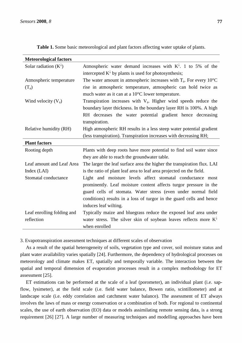
with a relative humidity of 100%. Some basic factors affecting water uptake of plants are summarized
in Table 1.
Water stress affects plant yield by a reduction of leaf area, a reduction of stomatal conductance, by a
reduction of CO2 uptake and hence photosynthesis and by a slow down of root elongation and
development. Water stress also affects proper seed development (starch filling). Yield and water stress
can be quantified with the concept of Water Use Efficiency (WUE). The physiological definition of
WUE is: “The amount of carbon in milligrams of assimilated carbon per gram of H2O transpired”. The
agronomist defines WUE as: “The ratio of dry matter produced (yield) to water consumed”.
Crassulacean Acid Metabolism (CAM) plants are metabolically optimized for the highest WUE
compared to C3 and C4 metabolism plants. CAM plants can close their stomata during daytime and
open them at night. This strategy ensures a significant reduction of water loss by reduced transpiration.
CAM plants have a low and variable productivity but a very high WUE.
In general C4 species elicit a higher WUE than C3 plants. Typically C4 plants can close their
stomata (less CO2 and less water loss) during daytime, while still carrying out a high level of
photosynthesis. Evidently this leads to a higher WUE than C3 plants, which do not have this capacity.
Sensors 2008, 8
77
Table 1. Some basic meteorological and plant factors affecting water uptake of plants.
Meteorological factors Solar radiation (K↓) Atmospheric water demand increases with K↓. 1 to 5% of the
intercepted K↓ by plants is used for photosynthesis;
Atmospheric temperature
(Ta)
The water amount in atmospheric increases with Ta. For every 10°C
rise in atmospheric temperature, atmospheric can hold twice as
much water as it can at a 10°C lower temperature.
Wind velocity (Va) Transpiration increases with Va. Higher wind speeds reduce the
boundary layer thickness. In the boundary layer RH is 100%. A high
RH decreases the water potential gradient hence decreasing
transpiration.
Relative humidity (RH) High atmospheric RH results in a less steep water potential gradient
(less transpiration). Transpiration increases with decreasing RH;
Plant factors
Rooting depth Plants with deep roots have more potential to find soil water since
they are able to reach the groundwater table.
Leaf amount and Leaf Area
Index (LAI)
The larger the leaf surface area the higher the transpiration flux. LAI
is the ratio of plant leaf area to leaf area projected on the field.
Stomatal conductance Light and moisture levels affect stomatal conductance most
prominently. Leaf moisture content affects turgor pressure in the
guard cells of stomata. Water stress (even under normal field
conditions) results in a loss of turgor in the guard cells and hence
induces leaf wilting.
Leaf enrolling folding and
reflection
Typically maize and bluegrass reduce the exposed leaf area under
water stress. The silver skin of soybean leaves reflects more K↓
when enrolled
3. Evapotranspiration assessment techniques at different scales of observation
As a result of the spatial heterogeneity of soils, vegetation type and cover, soil moisture status and
plant water availability varies spatially [24]. Furthermore, the dependency of hydrological processes on
meteorology and climate makes ET, spatially and temporally variable. The interaction between the
spatial and temporal dimension of evaporation processes result in a complex methodology for ET
assessment [25].
ET estimations can be performed at the scale of a leaf (porometer), an individual plant (i.e. sap-
flow, lysimeter), at the field scale (i.e. field water balance, Bowen ratio, scintillometer) and at
landscape scale (i.e. eddy correlation and catchment water balance). The assessment of ET always
involves the laws of mass or energy conservation or a combination of both. For regional to continental
scales, the use of earth observation (EO) data or models assimilating remote sensing data, is a strong
requirement [26] [27]. A large number of measuring techniques and modelling approaches have been
Sensors 2008, 8
78
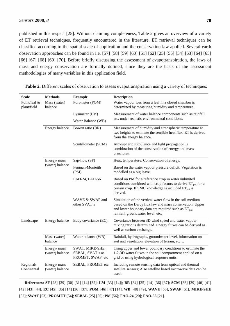
published in this respect [25]. Without claiming completeness, Table 2 gives an overview of a variety
of ET retrieval techniques, frequently encountered in the literature. ET retrieval techniques can be
classified according to the spatial scale of application and the conservation law applied. Several earth
observation approaches can be found in i.e. [57] [58] [59] [60] [61] [62] [25] [55] [54] [63] [64] [65]
[66] [67] [68] [69] [70]. Before briefly discussing the assessment of evapotranspiration, the laws of
mass and energy conservation are formally defined, since they are the basis of the assessment
methodologies of many variables in this application field.
Table 2. Different scales of observation to assess evapotranspiration using a variety of techniques.
Scale Methods Example Description
Point/leaf & plant/field
Mass (water) balance
Porometer (POM) Water vapour loss from a leaf in a closed chamber is determined by measuring humidity and temperature.
Lysimeter (LM)
Water Balance (WB)
Measurement of water balance components such as rainfall, etc. under realistic environmental conditions.
Energy balance Bowen ratio (BR) Measurement of humidity and atmospheric temperature at two heights to estimate the sensible heat flux. ET is derived from the energy balance.
Scintillometer (SCM) Atmospheric turbulence and light propagation, a combination of the conservation of energy and mass principles.
Energy/ mass (water) balance
Sap-flow (SF) Heat, temperature, Conservation of energy.
Penman-Monteith (PM)
Based on the water vapour pressure deficit. Vegetation is modelled as a big leave.
FAO-24, FAO-56 Based on PM for a reference crop in water unlimited conditions combined with crop factors to derive ETpot for a certain crop. If SMC knowledge is included ETact is derived.
WAVE & SWAP and other SVAT’s
Simulation of the vertical water flow in the soil medium based on the Darcy flux law and mass conservation. Upper and lower boundary data are required such as ETpot, rainfall, groundwater level, etc.
Landscape Energy balance Eddy covariance (EC) Covariance between 3D wind speed and water vapour mixing ratio is determined. Energy fluxes can be derived as well as carbon exchange.
Mass (water) balance
Water balance (WB) Rainfall, hydrographs, groundwater level, information on soil and vegetation, elevation of terrain, etc…
Energy/ mass (water) balance
SWAT, MIKE-SHE, SEBAL, SVAT’s as PROMET, SWAP, etc
Using upper and lower boundary conditions to estimate the 1-2-3D water fluxes in the soil compartment applied on a grid or using hydrological response units.
Regional/ Continental
Energy/ mass (water) balance
SEBAL, PROMET etc Including remote sensing data from optical and thermal satellite sensors; Also satellite based microwave data can be used.
References: SF [28] [29] [30] [31] [14] [32]; LM [33] [14]); BR [34] [35] [14] [36] [37]; SCM [38] [39] [40] [41]
[42] [43] [44]; EC [45] [35] [14] [36] [37]; POM [46] [47] [14]; WB [48] [49]; WAVE [50]; SWAP [51]; MIKE-SHE
[52]; SWAT [53]; PROMET [54]; SEBAL [25] [55]; PM [56]; FAO-24 [20]; FAO-56 [21].
Sensors 2008, 8
79
3.1. The conservation laws
A typical, daily one-dimensional water (mass) balance equation can be defined as follows:
0 S -D -R -ET -Irr CR P =++ (5)
In Eq. (5):
P is the amount of rainfall [mm d-1];
CR is the capillary rise from the groundwater table [mm d-1];
Irr is the irrigation dose [mm d-1];
ET is evapotranspiration [mm d-1];
R is runoff [mm d-1];
D is drainage [mm d-1];
and S is the storage of water in the soil compartment [mm d-1].
A typical, daily one-dimensional energy balance omits (or ignores) energy storage in the canopy due
to photosynthesis. For a vegetated land surface, the energy balance equation can be written as:
0 λE-H -S-G -R 0n = (6)
In Eq. (6):
Rn is net radiation (net short and net long wave) [W m-2];
G0 is the subsurface heat flux [W m-2];
S is the rate of heat storage in the plant canopy [W m-2];
H is the sensible heat flux [W m-2];
λE is the latent heat flux [W m-2];
λ is the latent heat of vaporization of water, approximately 2,450 J g-1 H2O at 20°C;
and E is evapotranspiration [g H2O m-2 s-1].
The energy storage due to photosynthesis is generally estimated to be less than a few percent of land
surface net radiation [71]. Hence, generally the energy storage term S in the equation of the land
surface energy balance is omitted. However, heat storage in plant canopies can become a substantial
part of the energy balance for periods less than a day, particularly for massive canopies such as those of
forests. Quantitative information on S is rare in the literature however and moreover difficult to obtain
[49]. Both mass and energy balances can be combined, for example by estimating ET using the energy
balance, it is possible to better estimate the other terms of the water balance like for example water
drainage.
3.2. Point / leaf / plant and field scale transpiration and evapotranspiration estimation
The execution of field measurements represents a labour intensive endeavour. Moreover, it is a time
consuming activity, which generally requires expensive equipment. In situ, potentially everything can
Sensors 2008, 8
80
go wrong. Despite these caveats, field measurements are the very touchstone to confront a modelling
approach with the physical reality of the environment. Field measurements provide a treasure of
information for the validation of models and for accurate quantitative information needed and asked for
by policy and decision makers. Models without accompanying measurements, i.e. calibration and
validation (cal/val) data, may be sophisticated mind constructions but they are worthless for sure in
underpinning land management policy making. In the next chapter, we give a short overview of sap-
flow sensors, the porometer, the lysimeter and field water balance approaches. These techniques
produce consistent temporal profiles of ET data with a local outreach.
3.2.1. Estimation of transpiration based on Sap-flow measurements
A sap-flow sensor involves heater and temperature probes which are inserted into stems or
branches. Sap-flow absorbs heat thereby inducing a temperature drop. Different type of sap-flow
measurement principles exist. For instance the Heat Pulse Velocity principle is applied with a heater
probe inserted into the sapwood, with thermocouples inserted downstream and sometimes upstream of
the sensor to measure temperature change due to the heat pulse. The Thermal Dissipation Probe is
applied by insertion of an upper needle containing a heater element and a thermocouple which is
referenced to a second needle downwards in the sapwood stream. The Heat Field Deformation Method is applied by the use of a heater and two atmospherics of a thermocouple implanted
symmetrically and asymmetrically into the stem. The Heat Balance Method is based on the ratio
between heat input and temperature rise in a pre-defined space. Finally, the Stem Heat Balance method is applied by external heating with a soft and flexible heater and a couple of thermo-sensors.
These techniques allow, to measure plant effective water streams. In that respect sap-flow sensors
are very useful for calibration and validation of water and energy balance algorithms whether or not
based on remote sensing. They are a very good alternative to lysimeter experiments. Operation of sap-
flow sensors though, requires a vast technical input and maintenance effort. Power supply in areas
without electricity distribution is an evident problem. Signal conversion (from temperature to sap-flow)
involves a (semi)-empirical approach and is based on a priori knowledge of the sapwood basal area.
Sapwood basal area is required to convert flow velocities to transpiration rates. Moreover, water
storage in the stem must be considered. Tree dimensions are needed for the up-scaling from stem at
breast height to the tree level (hence, tree characteristics must be known). More information on the
techniques described can be found in: [72] [30 [31] [28] [29] [32] [14].
3.2.2. Estimation of transpiration based on Porometer measurements
A porometer measurement estimates transpiration of a leaf or twig by measuring:
(i) the increase of humidity within a closed chamber attached to the leaf, or;
(ii) with a steady state porometer that maintains a constant humidity in a measuring chamber by
matching a flow of dry atmospheric to balance water vapour loss from the enclosed leaf.
Water vapour loss from the chamber by atmospheric flow equals the gain in water vapour by
transpiration (mass conservation principle). The instrument calculates the amount of water
vapour outflow from measured atmospheric flow, relative humidity, and temperature and
corrects for the known leaf area in the cuvette to give transpiration per unit leaf area.

Sensors 2008, 8
81
Porometers are used to determine leaf stomatal conductance but one may also be tempted to
extrapolate measurements on a single leave to a whole canopy, when knowing total leaf area.
A porometer measurement provides direct estimates of water loss from leaves. It suffers however
from the requirement that the estimations at leaf level must be extrapolated to a whole canopy. This
type of up-scaling is not straightforward. Transpiration rates measured with a porometer do not
correspond with those measured in undisturbed natural conditions. This is due to differences in
boundary layer conductance. A more rigorous approach is the independent determination of
atmospheric saturation deficit and the transpiration rate by porometry [73] thereby taking boundary
layer conductance into account. Porometers are useful for conductance-based models since leaf
stomatal conductance and transpiration can be measured. More specific information on this topic can
be found in [46] [47] [14].
3.2.3. Estimation of evapotranspiration based on a lysimeter
The lysimeter is widely used in laboratories and for field work, mainly for agronomic research. The
weighing lysimeter technique can be extended if there is a requirement for measurements of tree
transpiration. An undisturbed vegetated soil sample is taken with cylinders of different diameters (up to
3.14 m2). ET is estimated from the mass balance of water of initial minus final weight plus rainfall
minus drainage.
The main advantage of lysimeter in situ measurements is that water consumption of vegetation can
be performed under approximately realistic field conditions. However, a lysimeter measurement
requires elaborate preparation in fact intrinsic to field measurements. Moreover it is typically limited to
only few individual trees or a small surface area of agricultural crops. Additionally only young trees
can be measured, hence this type of measurement is not representative for aged or mixed age forest
stands. Moreover, the installation of lysimeters can cause disturbances compared to surrounding
vegetation and agricultural crops in a lysimeter may suffer from a different treatment than crops in the
field. A more realistic approach is the ‘natural lysimeter’ [74]. In this type of lysimeter, a barrier to
lateral water flow in and above the soil is installed and measurements of precipitation and soil water
content are made while the rate of deep drainage is approximated.
The lysimeter is very useful for data collection and for modelling water use and growth of
agricultural crops. Also known is chemical solute transport research. More specific information can be
found in [33] [31] [75].
3.2.4. Estimation of evapotranspiration based on the Bowen ratio
The Bowen ration (BR) is a micrometeorological variable evaluated for a height of a few meters to a
few tens of meters above a surface, representative for the surface sub-layer of the atmospheric
boundary layer. Under steady state conditions and in absence of horizontal gradients of vertical fluxes
of momentum, heat, and water vapour flux, the vertical fluxes of heat and water vapour within a fully
turbulent surface sub-layer are not appreciably different from these fluxes at the earth’s surface [76].
The scalar vertical fluxes of heat and water vapour of land or water surfaces are estimated within the
surface sub-layer. Typically, the Bowen ratio is an energy balance method and represents the ratio of
the sensible and latent heat fluxes. The BR is variable used in a widespread approach for ET
Sensors 2008, 8
82
determination at the local scale. An important boundary condition, however for the evaluation of a one-
dimensional BR, is the absence of horizontal energy fluxes. Hence, it cannot be used inside canopies.
Furthermore, net radiation and soil heat fluxes must be measured simultaneously. With the BR
approach, ET can be estimated beyond the point scale and can therefore be used to compare and
classify vegetation types. More specific information about this approach can be found in [35] [37] [14]
[36].
3.2.5. Estimation of evapotranspiration based on meteorological datasets
Estimation of ET can be based on energy balance schemes and the Penman-Monteith [56] equation
in one of its many varieties. ET estimation can be based as well on the parameterization of energy
balance components. Both the Penman-Monteith (PM) equation and the parameterization can be
implemented in combination with EO assimilation techniques. In many approaches ETact is estimated
from ETpot (i.e. obtained from water balance models such as WAVE see next section); energy balance
models such as Penman-Monteith and derivates. A formal definition of ETpot was already given in
section 1.2. The formulae to estimate ETpot for other vegetation than lawns is based on ETref and (Kc)
as mentioned below (FAO-56 procedure).
The Penman-Monteith equation is applied within the concept of a ‘big-leaf’ approach and evaluates
ET from the energy balance, combined with mass transfer. Since in the 1950’s and 60’s surface
temperature could not be measured accurately, hence atmospheric-surface temperature differences
could not be applied to calculate sensible heat fluxes. The Penman equation for open water however
does not pose problems, since for this surface type atmospheric and water surface temperatures are
assumed to be quasi equal. This is in contrast with the case of vegetation and bare soils.
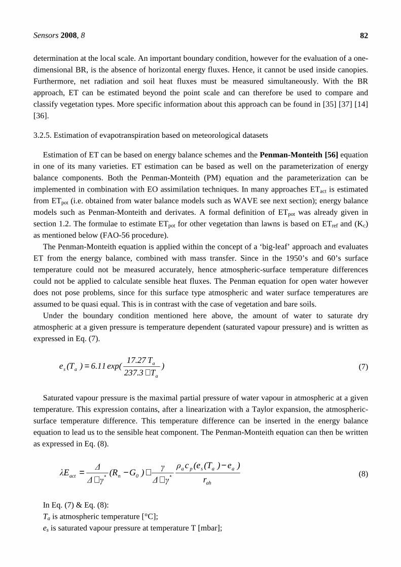
Under the boundary condition mentioned here above, the amount of water to saturate dry
atmospheric at a given pressure is temperature dependent (saturated vapour pressure) and is written as
expressed in Eq. (7).
)T237.3
T 17.27exp( 6.11)(Te
a
aas +
= (7)
Saturated vapour pressure is the maximal partial pressure of water vapour in atmospheric at a given
temperature. This expression contains, after a linearization with a Taylor expansion, the atmospheric-
surface temperature difference. This temperature difference can be inserted in the energy balance
equation to lead us to the sensible heat component. The Penman-Monteith equation can then be written
as expressed in Eq. (8).
ah
aaspa
0nact r
)e)(T(ecρ
γ∆
γ)G(R
γ∆
∆λE
−
++−
+= ∗∗ (8)
In Eq. (7) & Eq. (8):
Ta is atmospheric temperature [°C];
es is saturated vapour pressure at temperature T [mbar];

Sensors 2008, 8
83
∆ is the slope of the vapour pressure curve [mbar K-1];
γ* equals γ (1+rc rah-1);
γ is the psychrometric constant [mbar K-1];
(es(T0)-ea) is saturated vapour pressure deficit [mbar];
rah and rc respectively are the aerodynamic and canopy or surface resistances according to the ‘big
leaf’ concept expressed in [s m-1]; Generally rc is defined as rs LAI -1 where rs is the stomatal resistance
of leaves.
A simplification of the Penman-Monteith equation is the Priestley-Taylor equation [77]. These
authors stated that the atmospheric drying power over a wet surface is a constant, multiplied with ∆(Rn-
G0) as expressed in Eq. (9).
γ∆
∆)G(R αλE 0n +
−= (9)
α is a constant [-] ranging from 1 to 1.35 for wet surfaces [78];
γ is the psychrometric constant [mbar K-1];
∆ is the slope of the vapour pressure curve [mbar K-1].
Choisnel et al. [19] mentions an expression derived from the Penman-Monteith equation, Makkink
(1957). It is used in the Netherlands with α taking a value of 0.65 (or 0.8 times of its value in the
Penman expression in Eq. (9). Brochet-Gernier used the same expression for France [19].
For sparse canopies, the Penman-Monteith ‘big-leaf’ approach no longer holds. Under these
boundary conditions, soil evaporation must be incorporated in the modelling approach. Shuttleworth &
Wallace [79] suggested the use of a resistance model. In that approach, the energy available for
evaporation from the canopy and soil compartments is calculated first and subsequently a resistance
model is used to estimate the fluxes between soil and vegetation.
Insertion of the parameters of a hypothetically well watered lawn (height: 0.12 m; surface resistance:
70 s m-1; albedo: 0.23) into the Penman-Monteith equation, allows to evaluate ETref. With ETref, ETpot
and ETref for a specific crop is calculated according to crop factors (Kc) used in Eq. (10). A typical Kc
value during the mid-summer season for many cereal crops is 1.15 [21]). For forest trees between it is
situated between 0.7 and 1.1 (as derived with the WAVE model, [80]).
In the FAO-56 approach [21], a dual crop coefficient is use, which takes a dry soil surface layer and
adequate soil water content (SMC) in the root compartment into account for full transpiration
evaluation. Root zone moisture depletion is evaluated as the difference between SMC at field capacity
(pF = 2.3) and actual SMC. The Ks value (which is a water stress factor) equals 1.0 as long as SMC is
higher than readily available water (a fraction of the total available water). If SMC is lower than readily
available water (RAW), Ks decreases linearly from one to zero according to total available soil water
consumed. The FAO-56 procedure is a revised FAO-24 version [20].

Sensors 2008, 8
84
refccrop ET K ET = (10)
refcscrop act, ET K K ET = (11)
In Eq. (10) & Eq. (11):
Kc is a crop factor [-];
ETref is reference crop ET [mm d-1];
ETpot is potential crop ET [mm d-1];
Tact crop is crop ET under water stress conditions [mm d-1];
Ks is a stress factor [-].
Xu & Singh [81] evaluated and generalized temperature and radiation based methods for ETpot
estimation. Most equations adopting this methodology, take the same shape as Eq. (10) & (11). The
following methods have been evaluated (see [81]): Thornthwaite (1948), Linacre (1977), Blaney and
Criddle (1950), Hargreaves (1975), Kharrufa (1985), Hamon (1961) and Romanenko (1961). Singh &
Xu [82] evaluated and compared 13 ET equations belonging to the category of the mass transfer
methods and developed a generalized model. They also examined the sensitivity of the equations to
errors in daily and monthly input data [81].
aapot cT ET = (12)
h)c-(cTdc ET 32a11pot = (13)
baR ET gpot += (14)
In Eq. (12), Eq. (13) & Eq. (14):
ETpot is the potential evapotranspiration [mm d-1];
Ta is atmospheric temperature [°C];
h is a humidity term [-];
d1 is day length [hours];
c, a, b, c1, c2, c3 are coefficients [-].
Rg is daily global radiation [MJ d-1 m-2].
3.2.5. Estimation of evapotranspiration based on field water balance methods
Field water balance methods are based on in situ measurements of hydrological mass fluxes. ET in
this approach is calculated as a residual of all the other terms of the field mass balance equation. With
pluviometers rainfall rate is measured, Time Domain Reflectometry [83] or other sensors (see section
4, Table 4) when inserted into different soil layers are used to determine soil moisture dynamics.
Tensiometers or groundwater level tubes, give an estimate of the lower boundary of the soil
compartment.
Note that the results obtained are very sensitive to measurement frequency differences and the
amount of measurement locations, especially for the field scale spatial level. Field water balance

Sensors 2008, 8
85
methods are useful typically to obtain tree crop factors (popular [48]). More specific information about
this approach can be found in [48] [49].
In addition to the measurement of hydrological components to estimate ET, 1D models can be used
to simulate vertical water flow. The Darcian flux law for example states that a water flux in a
homogeneous porous medium equals the product of the hydraulic gradient and hydraulic conductivity.
When combined with the law of mass conservation, the well know Richard’s equation is obtained. This
equation can even be extended to 3D conditions and describes the water flux into soils. Typical 1D
models are WAVE (Water and Agrochemicals in the Vadose Environment [50]) and SWAP [51]. ET is
modelled using inputs like rainfall, interception capacity and a (grass) reference potential
evapotranspiration as the upper boundary condition. The major lower boundary condition is the
groundwater table or the drainage flux. Additional inputs are crop factors, root distribution, leaf-area-
index and critical pressures for water uptake. The soil system is described using its soil physical
properties like the hydraulic conductivity and retention curves according to the corresponding soil
layer. Obviously, 1D modelling corresponds with the field water balance method discussed earlier.
To estimate ET with a 1D water balance model, canopy interception is calculated first using
interception capacity. When the amount of gross rainfall is larger than canopy capacity, excess
rainwater will reach the soil surface. Rainwater mass equal or smaller than interception capacity is
assumed to evaporate. Depending on the maximum infiltration rate of the upper soil, runoff may occur
while the remainder of rainwater infiltrates into the lower soil layers of the soil compartment. The
product of ETref and the crop factor (Kc) of the vegetation considered results in ETpot, i.e. the maximum
rate of water consumption under a non-stress boundary condition. Using leaf-area-index (LAI) in
Beer’s law, ETpot is split into potential soil evaporation and crop transpiration. This potential crop
water use in combination with crop root distribution and SMC, determines the amount of water
extracted from the soil compartment. If SMC is smaller than the moisture amount required according to
potential water use, then the actual water use is obtained. Actual soil evaporation is calculated from
water stress in the topsoil. Non evaporated water is stored in the soil while excess water (not stored),
will drain into the deeper under-field. In case of capillary rise, more water will reach the root zone and
less water stress occurs.
Although ETact is determined using a water balance approach, ETpot must be calculated first,
generally by applying the Penman-Monteith relationship or its derivates. A description and
implementation of the WAVE model to estimate ET of Flemish forest can be found in [80]. The spatial
up-scaling of 1D models is possible by input of the upper and lower boundaries in a spatially explicit
mode. In that case, soil physical properties are required to be input in 3D mode. 3D models must also
be able to account for unforeseen water fluxes.
3.3. Evapotranspiration estimation at the field, landscape, regional and continental scales
Where local estimates of ET are satisfactory needed, typically for validation purposes or where
detailed small scale application, many applications require spatially up-scaled ET maps. Rather well
adapted techniques for this objective are the Bowen ratio, eddy correlation, the scintillometer and field
water balance methods.
Sensors 2008, 8
86
3.3.1. Scintillometer measurements
A scintillometer measurement is based on the physical principle of the propagation of
electromagnetic waves in atmospheric and their disturbance by atmospheric turbulence. This
turbulence effect induces the so-called scintillation of the electromagnetic wave. It is the result of
fluctuations of atmospheric temperature, moisture, pressure and their interactions. Basically a
scintillometer measures the variance of radiation intensity fluctuations. An area-averaged sensible heat
flux can be derived from this type of measurements. The scintillometer consists of a transmitter
equipped with disc shaped arrays of light emitting diodes and a receiver, which records the perturbed
light at a distance up to 5 km. Latent heat is to be derived from the energy balance.
Scintillometers are applied to estimate turbulence as well. Typically the turbulence parameters are
the turbulent heat and momentum fluxes, the Monin Obukhov length (see also, the chapter on energy
flux based ET assessment method), the dissipation rate of energy, and the vertical distribution of
atmospheric temperature and finally refractive index. More specific information on the approach
described is found in [38] [39] [40] [41] [42] [43] [44].
3.3.2. Eddy covariance (EC) methodology
Basically, wind vector fluctuations in the three dimensions and in the constant flux region (lowest
section of the inertial sub-layer where the fluxes of momentum and heat, water vapour, and other gases
are constant with height) of the atmospheric surface boundary layer are measured with very short time
intervals. Combined with the associated fluctuations in atmospheric temperature, humidity, or mixing
ratios of typically, water vapour or carbon dioxide, the average net flux of the physico-chemical
variables mentioned is obtained by integrating their instantaneous fluxes. These fluxes are obtained by
evaluating the means, variances and co-variances of the vertical wind vector with its horizontal wind
counterpart, with sonic temperature (which is approximately equal to virtual temperature), with water
vapour as well as carbon dioxide mixing ratios.
A 3D sonic anemometer is used to obtain the orthogonal wind vectors and sonic temperature. A
folded, open path H2O/CO2 infrared gas analyzer is used to measure water vapour and carbon dioxide
mixing ratios. The application of footprint theory is required to produce a spatial representation of
evapotranspiration. Spatially explicit carbon dioxide fluxes can be derived accordingly. Needless to
stress the importance of this type of output for the calibration and validation of carbon balance models.
Eddy covariance is a very accurate method. It requires delicate planning with respect to obtaining
reliable instrumentation, calibration procedure, the determination of the exact measurement height
above the surface exchanging water vapour and carbon dioxide in relation to the required fetch, the
length of the sampling period etc. [84]. EC system management and logistical support is expensive and
time consuming, both from the point of infrastructure as human resources needed. The technique
however due to its accuracy and importance is widely applied for the determination and monitoring of
energy components and carbon dioxide and water vapour mass fluxes. Tower networks include for
instance the EUROFLUX towers in Europe [49], united at the global scale with other continental scale
networks in FLUXNET, the global eddy covariance tower network. More specific information is found
in [45] [35] [14] [36] [37].
Sensors 2008, 8
87
3.3.3. Catchment scale water balance methodology
With a hydrograph, instantaneous discharge can be measured and consequently, this enables the
calculation of annual runoff by dividing the total annual discharge with the surface area of the entire
watershed. Annual ET, integrated over the entire water catchment surface area, is then estimated as the
residual of total annual rainfall and total runoff. Although this method appears to lead to rather rough
EF estimates, Wilson et al. [49] for example found that the magnitude of annual ET estimated over 5
years (1995-2000) is in good agreement between the EC and the catchment water balance methods for
a catchment in the South-East of the USA. A major advantage of the catchment scale approach is that
only a limited amount of information sources (annual discharge, precipitation, area) is needed.
However, some other boundary conditions for use of this method are less favourable. For example, the
approach is only applicable for coarse time resolutions such as one year. Moreover an area-averaged
estimate is obtained. The field water balance method is typically used in combination with physical and
empirical (regression) computer models. More specific information is found in [85] [49].
3.4. Introduction of Earth Observation technology to quantify evapotranspiration
3.4.1. Energy flux measurements
A primordial observation from earlier sections in this paper is, that both SMC and ET, as spatially
as well as temporally variable processes, are measured and/or modelled based on the law of mass
and/or energy conservation. Since EO provides spatially explicit as well as multi-temporal information
on reflected or emitted electromagnetic radiation from the earth’s surface, appropriate techniques to
assess area ET and SMC is based on remote sensing [11].
The Planetary Boundary Layer (PBL) is that part of the atmosphere where the influence of land
surface densities is elicited. Considering the Planetary Boundary Layer (PBL) and especially its lower
atmospheric part or Atmospheric Surface Layer (ASL), the estimation of energy balance components
are related to the flux-profile as for instance measured with the eddy covariance. The different fluxes
under consideration are:
ah
az0hpa r
TTcρH
−= (15)
)q(qcρλE az0hpa −= (16)
sh
s0ss0 r
TLSTcρG
−= (17)
↑↓↑↓ −+−= LLKKRn (18) 40000n σLSTεLε)Kα(1R −+−= ↓↓ (19)
In Eqs. (15) to (19):
H, λE, G0 and Rn are sensible and latent heat, the soil flux and
the net radiation flux respectively [W m-2];
ρa and ρs are respectively the atmospheric and soil bulk densities [kg m-3];

Sensors 2008, 8
88
cp, cs are the specific heat of atmospheric at a constant pressure and soil specific heat [J kg-1 K-1];
rah and rsh are the resistance to heat transfer for atmospheric and soil respectively [s m-1];
Ta, Tz0h, Ts and LST0 are respectively atmospheric, heat source, soil and land surface temperatures
[°C];
qa and qz0h are respectively atmospheric humidity and humidity at reference height [-];
K↓ and K↑ are incoming and outgoing short wave radiation [W m-2];
L↓ and L↑ are incoming and outgoing long wave radiation [W m-2];
α0 is surface albedo [-];
ε0 is surface emissivity [-];
σ is the Stefan – Boltzmann constant [W m-2 K-4].
For homogeneous land surfaces flux-profile relationships are introduced using the similarity
hypothesis for wind, temperature and humidity vertical profiles.
The similarity hypothesis implies that:
(i) Flux densities are linearly related to the gradients of these parameters;
(ii) Flux densities of momentum, moisture and heat vary less than 10% with height and finally;
(iii) Buoyancy effects on before mentioned densities can be accounted for by one dimensionless
variable.
Shear stress is induced when a land surface is not smooth. Since kinetic (wind) energy is lowered by
surface friction, a compensating energy flux originates, which is the vertical flux density of
momentum. The typical shape of a wind speed profile e.g. according to the natural logarithmic of
height in a neutral atmosphere is well known. Of course, both forced and thermal convection do occur,
hence mixed convection occurs as well. At this point the Monin-Obukhov length scaled for mixed
convection is introduced. An equivalent temperature profile can also be derived. This profile generates
the scaling parameters for momentum and heat, in relation to their flux densities. This makes it
possible to convert measured wind speed and/or atmospheric temperature under given environmental
conditions into scaling parameters and their respective flux densities.
A typical approach for the representation of the scaling parameter of a wind profile is determined by
the use of resistance schemes for homogeneous individual land surface elements. For the sensible heat
flux density the resistance rah to heat transfer between zoh and a reference height zsur is related to the
eddy diffusion coefficient and more explicitly to wind speed. Analogous, the resistance to sensible heat
transport in the soil can be written as rsh. For latent heat, resistance parameters can be implemented as
well, but an appropriate choice of their values is problematic. Since land surfaces are generally not
homogeneous, resistance schemes have to be adjusted to represent surface heterogeneity, either by
implementing a one-layer scheme with effective system parameters or a multi-layer scheme with
separate parameters according to land surface characteristics. The second solution requires many
additional coefficients, difficult to obtain. Bastiaanssen [86] concluded from a literature review, that a
one layer resistance scheme is quite convenient to be applied.
A theoretical link between evapotranspiration derived from the energy balance equation and EO can
be made assuming the next boundary conditions [86]. Based on equations 15-19 and when Tz0h equals

Sensors 2008, 8
89
LST0, the surface energy balance for a specific location at a pre-defined moment in time can be
combined as follows, to obtain:
)Tr
cρT
r
cρ()LST
r
cρLST
r
cρ LSTσ(ελELε K)α(1 s
sh
ssa
ah
pa0
sh
ss0
ah
pa40000 +−++=−+− ↓↓ (20)
After the application of a first order Taylor expansion on the term ε0σLST04 and after re-expressing
the equation into LST0 [86] we obtain:
2
0010 c
λELε K)α(1cLST
−+−+=↓↓
(21)
Further reductions lead to Eq. (22):
λEccLST 430 −= (22)
Eq. (22) implies that evaporation is a linear combination of surface temperature. The different
coefficients ci can be derived using basic mathematical rules. The art of remote sensing is in this
specific case, the identification of the spatial patterns of c3 and c4 during a satellite (or aircraft)
overpass. Eq. (22) is the basis of quite a few methods applied to model the spatio-temporal patterns of
evapotranspiration.
3.4.2. Remote sensing based assessment of evapotranspiration
To exhaustively review existing remote sensing (RS) or field scale based approaches to determine
ET is a time consuming task indeed. We gladly refer to [87] and other authors for their evaluations of
remote sensing applications in the field of water resources management. Since a review on ET will
hardly ever be complete, this paper covers a limited list of remote sensing techniques assessing ET as
listed in Table 3. The advantages as well as disadvantages of the methods considered are indicated in
Table 3. Apart from the parameterization of the surface energy balance, other approaches are based on
a combination of the water balance approach, remotely sensed surface temperature and vegetation
retrievals. Another frequently applied approach is based on a combination of the Penman-Monteith
equation and RS data assimilation. Hence, the methods listed in Table 3 can be classified according to
whether they are based on:
(i) the parameterization of the surface energy balance;
(ii) the Penman-Monteith equation;
(iii) the water balance approach, or;
(iv) relationships between vegetation indices and land surface temperature assessed with remote
sensing.
A short description of the methods is given in the text below. From Table 3, one can conclude -
when generalizing - that most methods to assess ET with remote sensing require non-uniform surfaces
in the region of interest (ROI).

Sensors 2008, 8
90
Table 3. A limited list of evapotranspiration assessment methods based on Earth Observation
techniques. A summary of (some) model parameters is given, as well as model (dis-)advantages.
Concept Method Parameters Advantages Disadvantages Ref
(Sel.) EO Other
Par
amet
eris
atio
n of
the
ene
rgy
bala
nce
SEBAL LST,
α0,
NDVI
Ta, va, ε0, RH,
surface
roughness
Data requirements are minimal;
Physical concept; no need for land
use; multi-sensor approach.
Dry and wetland requirement to
estimate H, hence heterogeneous
surface needed in the ROI; only
applicable for flat terrain.
[88],
[89],
[90],
[25].
SEBS LST,
α0,
NDVI
Ta, va, ε0, LAI, ea
& esat,, surface
roughness
No a-priori knowledge of the
actual turbulent heat fluxes needed.
Dry and wetland requirement to
estimate H; combined with Penman-
Monteith equation.
[68],
[70].
RMI LST,
α0
Detailed
meteorological
data
Based on geostationary satellites
with high temporal resolution.
Monin-Obukhov lengths require
detailed meteorological data (network
of synoptical stations).
[64].
S-SEBI
iNOAA
LST,
α0,
NDVI
Ta, ε0, (RH) Data requirements are minimal; No
need for land use; no need to
estimate H, multi-sensor.
Dry and wetland requirement to
estimate evaporative fraction
(dependent on ROI).
[91],
[69].
Pen
man
-Mon
teit
h ba
sed
Trapezo-
idal
shape
LST,
SAVI
Ta, ε0, vapour
pressure deficit,
LAI
Minimal meteorological data
requirement, ET estimation at
regional scales.
Requirement for biome map, surface
roughness, vegetation height.
[92].
Promet α0, Resistance
values, LAI, soil
type
Across scales, physiologically based
(SVAT).
Requires a plant physiological
model, land use, extensive
meteorological dataset.
[54].
Granger LST,
α0,
NDVI
Ta, saturated
vapour pressure
Feedback relationship: LST is
used to obtain the vapour pressure
deficit in the overlying air.
Requires long term Ta and a
conventional ET model including
vapour transfer coefficient.
[65].
Wang LST,
α0, VI
Meteorological
data
Gradients of Ta and LST not
required.
Day and night LST required. [93].
Cleugh LST,
α0, VI
Meteorological
data
Linear relationship surface
conductance and MODIS-LAI.
Extensive meteorological data and
estimations of canopy cover required.
[94].
Wat
er b
alan
ce b
ased
SWAP α0, VI Meteorological,
soil, ground
water table data
A mechanistic model simulating
plant growth both temporal as
spatially (GIS, EO).
Requires extensive datasets.
Relationships between RS, vegetation
data, soil profile, groundwater fluxes.
[66]
Price LST,
VI
Meteorological,
soil, ground
water table data
Point method is extended spatially
based on pixels of completely
vegetated and bare soils.
Independent ET estimates required for a
completely vegetated area and for a
non-vegetated area; non-uniform area.
[58].
VI/
LST
bas
ed
Nagler EVI,
LST
Ta, calibration
coefficients
Simple and minimal input
requirements.
Need for site specific calibration, sensor
type sensitive.
[95],
[96].
Jackson LST
(VI)
Ta, (va,),
calibration coeff.
Simple relationship between VI and
LST. Minimal input datasets.
Calibration parameter depends on
surface roughness and wind speed.
[57].
EVI: Enhanced Vegetation Index.

Sensors 2008, 8
91
As indicated in Table 3, many methods are based on the use of the remote sensing criteria of dry and
wet pixels or vegetated and bare soils. Hence, spatially heterogeneous ROI ’s favours the application
of EO techniques. A rather trivial conclusion since otherwise point techniques would be sufficient
for the assessment of ET.
(i) Parameterization of the surface energy balance Bastiaanssen et al. [25] [55] developed the model, “Surface Energy Balance Algorithm for Land”
(SEBAL), which estimates energy partitioning at the regional scale with a minimal requirement for
field data. This algorithm is based on the use of surface albedo, a vegetation index and land surface
temperature and provides enough information for the parameterization of the energy balance fluxes,
e.g., radiation, sensible and soil heat as shown by [25] [55]. This algorithm has been applied in many
studies [88] to estimate ET, but also as a tool to estimate other components of the water balance at
large scales [97]. It is based on the parameterization of energy fluxes as indicated in this section. The
terms of the incoming radiation equation are based on field data and the outgoing terms on RS
estimated surface albedo, surface emissivity and land surface temperature. The soil heat flux is
estimated empirically, taking surface heating, soil moisture and intercepted solar radiation into
consideration. Sensible heat is computed from flux inversions for dry non-evaporating land units and
wet evaporating land surfaces. Roughness length is derived from an empirical vegetation index based
relation. ET is the residual of the energy balance. Lagouarde et al. [89] implemented the SEBAL model
over an agricultural area in the South–East of France. Eddy covariance (EC) measurements were
available. Large discrepancies between the reference sensible heat flux from EC and the SEBAL
derived flux were observed. This was attributed to errors in the estimates of roughness length based on
the use of a semi-empirical NDVI relationship. SEBAL estimates elicited a much closer fit with EC-
measurements using a prescribed roughness length for momentum.
Gellens-Meulenberghs [64] assessed ET as a residual of the energy balance using METEOSAT
imagery (albedo and land surface temperature) and meteorological and vegetation data. The energy fluxes are parameterized. The soil heat flux is a fraction of the net radiation flux and sensible heat. A
terrain dependent aerodynamic roughness parameter and displacement height values are both derived
from a digital land use map.
Regional Evapotranspiration through Surface Energy Partitioning (RESEP) has been proposed by
Ambast et al. [67] using boundary layer theory. ETact is estimated using the evaporative fraction (EF)
and 24 hourly net radiation. EF is also used in the Surface Energy Balance System SEBS [68]. For the
calculation of this fraction the concept of sensible and latent fluxes under dry-limited and wet-limited
conditions is used.
Verstraeten et al. [69] used evaporative fraction (EF) as a measure for ET. They derived EF from
remotely sensed albedo and land surface temperature. EF is the ratio of latent heat over the available
energy which indicates the amount of surface energy available for the evaporation of water [98].
García et al. [99] estimates EF with ASTER reflective and thermal data to estimate surface water
deficit. Senay et al. [70] developed and implemented a Simplified Surface Energy Balance (SSEB)
model to monitor and assess ETact and the performance of irrigated agriculture land using MODIS,
Sensors 2008, 8
92
ASTER and Landsat imagery. Kimura [100] estimated moisture availability using a combination the
NDVI and land surface temperature in a Modified Temperature-Vegetation Dryness Index (MTVDI).
(ii) Penman-Monteith combined with RS Moran et al. [92] combined the Penman-Monteith equation with land surface temperature and
spectral reflectance to estimate evaporation rates for a semi-arid grassland. This method is based on (a
hypothetical) trapezoidal shape of the relationship existing between the vegetation index and the
atmospheric-soil temperature difference (four vertices occur: 1. well-watered vegetation; 2. water-
stressed vegetation; 3. dry bare soil and 4. saturated bare soil). ET is assumed to be linearly associated
with temperature difference variations.
The PROMET model family assesses ET at field (1 ha), micro (100 km²) as well as meso-scale
(10.000 km²) [54] applying the Penman-Monteith algorithm and RS data assimilation. The
PROMET models combine a kernel (Penman-Monteith based SVAT) and a plant-physiological model
(to take environmental parameters and canopy resistance into account) and a spatial model. Surface
resistance is derived using a coupled plant physiological and soil hydraulic model. Stomatal resistance
is determined as a function of intercepted PAR. The 1st micro-scale model layer uses LANDSAT
imagery to determine land cover. The 2nd layer consists of spatially explicit soil information. The 3rd
layer is a meteorological time series and the final 4th layer contains plant developmental data (LAI,
height). For each image pixel a single set of parameters is implemented. The meso-scale model
requires NOAA/AVHRR imagery for sub-pixel information collection, with the boundary condition
that multi-temporal courses of reflectance and (thermal) emission as measured for each pixel are
linearly composed of reflectances and emissions for all land cover types, represented in the pixel.
Granger [65] used a mass transfer method with has its origin in the Penman-Monteith equation
applied within a remote sensing framework. He successfully used feedback mechanisms between land
surface and the atmospheric layer, so that the observed surface temperature is a sufficiently reliable
indicator of atmospheric humidity. A relationship between daily atmospheric vapour pressure deficit
and the saturated vapour pressure at the mean daily surface temperature was derived by this author. A
long-term mean atmospheric temperature site component is introduced to account for seasonal and
latitudinal effects.
Cleugh et al. [94] used the Penman-Monteith algorithm with LAI derived from MODIS satellite
data to model leaf conductance.
(iii) Water balance combined with RS With the integration of agro-hydrological and hydraulic simulation models as well as EO and GIS
techniques, D’Urso [66] developed a spatio-temporal irrigation management tool based on the water balance. SWAP is a combination of spatially extended upper and lower boundaries and soil system
conditions. For the upper boundary, meteorological data are assumed to be uniform and their spatial
distribution governed by canopy variables such as LAI, crop height, Kc and albedo. Kc coefficients are
mapped using satellite observations either using classification approaches (supervised and
unsupervised) validated with field observations or by formally defined analytical functions relating
reflectance to LAI, albedo and crop height. LAI is related to a vegetation index. The lower boundary is
Sensors 2008, 8
93
spatially extended using functions relating water flux at the bottom of the soil profile and the depth of
the groundwater table. The spatial distribution of soil hydraulic characteristics is obtained by
calibration of pedo-transfer-functions for the soil type units in a soil map and the functional properties
of the soil type. For example, the time required to reach a specified value of pressure head at a certain
soil depth. ETpot is calculated using Penman-Monteith.
The ALiBi model [101] is based on the mass transfer method as well. It makes use of vapour
pressure deficit in combination with a turbulent exchange coefficient and vegetation surface
conductance which depends on leaf stomatal conductance. Inversion of the model was performed by
Olioso et al. [102], with the retrieval of canopy ET from RS data including thermal infrared, spectral
reflectances and microwave data.
(iv) Direct relationships with remotely-sensed vegetation indices and land surface temperatures
Based on Eq. (22), ET is linearly related to land surface temperature. Jackson et al. [57] introduced
a simplified equation variant to estimate latent heat (Eq. (23):
)T-B(LST-G -RλE n
a00n= (22)
In Eq. (22):
n (close to one) and B are parameters dependent on land surface roughness and wind speed and can
be written as a function of a VI [103].
Moran et al. [104] applied the Temperature Vegetation Trapezoid (TVT) type of relationship. Qi et
al. [63] used the same approach combined with in situ measurements. Some years before [62], Price
[58] applied a relationship between a vegetation index and surface temperature to spatially upscale ET.
For heterogeneous land cover and based on the NDVI surface temperature relationship, three different
assumedly homogeneous terrestrial functional types (TFT) were defined. Well watered vegetated
pixels, dry and wet bare soils. Apart from the assumedly homogeneous TFT pixels, other pixel types
are assumed to be composed of a linear combination of the fractions of the three homogeneous cover
types, as previously defined. Similarly, Carlson et al. [59] [60] [61] combined a planetary boundary
layer model with surface temperature and NDVI measurements, to map soil moisture for the surface
and root zone.
4. Soil moisture content assessment techniques at different spatial observation scales
Despite the importance of soil moisture content, its accurate regional assessment is a complex issue.
This is mainly due to the fact that the standard estimation protocol, i.e., the gravimetric method, is
essentially a point measurement. To map local scale variations in soil moisture requires a high spatial
density of observation locations. Obviously point measurements performed in the context just
described is labour intensive and quite costly.
Other measuring techniques such as Time Domain Reflectometry (TDR) [83] are local
measurements as well, but not very suitable for the determination of the soil water status at field and
Sensors 2008, 8
94
regional scale as well. Earth observation based up-scaling techniques are a compromise since they are
spatially explicit and of relatively low cost [11] [13]. For instance, the spatial resolution of most
spaceborne sensors ranges from ± 30 m (Landsat ETM) to ± 250-500 m (MODIS) to ± 1100 m
(NOAA/AVHRR, MODIS) to ± 5000 m (METEOSAT) and even to ± 50000 m (ERS Scatterometer)
and more.
A general non-exhaustive list of methods to determine soil moisture at point and spatially explicit
scales, is given in Table 4, with a short description. According to the discussion of [105], well known
techniques to determine soil moisture content are
(i) Gravimetric techniques;
(ii) Nuclear (neutron scattering, gamma attenuation, nuclear magnetic resonance);
(iii) Electromagnetic (resistive and capacitive sensors, time and frequency domain reflectometer);
(iv) Tensiometric;
(v) Hydrometric;
(vi) Remote sensing (passive and active microwave, thermal infrared) and;
(vii) Optical techniques (polarized light, fibre optic sensors, near-infrared);
(viii) An additional technique, is the heat dissipation method [106] where heating or cooling of a
porous block is measured after a heat pulse;
(ix) Another, more basic field method is the ‘Feel and Appearance method’, using a soil moisture
interpretation chart based on texture classification and squeezing of soil samples [107].
Apart from RS techniques, all given techniques are point measurements. A summary of the advantages
and limitations of optical and microwave soil moisture remote sensing is provided by [3]. They made a
discussion on spectral measurements such as visible, NIR and SWIR reflectances, thermal infrared
emittance, microwave emission and radar measurements. Other methods to assess soil moisture content
are the implementation of calibrated and validated hydrological and SVAT models. Both one-
dimensional field (WAVE, SWAP see also Table 1) and distributed catchment models (SWAT [53];
MIKE-SHE [52], among others) can provide useful information. Gaps in time series of measured soil
moisture content can for example be reconstructed using the validated type of models, cited.
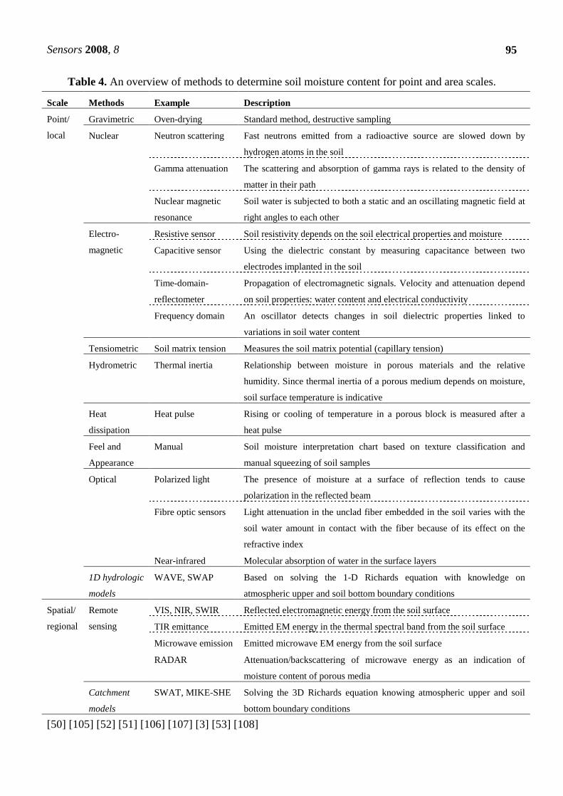
Sensors 2008, 8
95
Table 4. An overview of methods to determine soil moisture content for point and area scales.
[50] [105] [52] [51] [106] [107] [3] [53] [108]
Scale Methods Example Description
Point/
local
Gravimetric Oven-drying Standard method, destructive sampling
Nuclear Neutron scattering Fast neutrons emitted from a radioactive source are slowed down by
hydrogen atoms in the soil
Gamma attenuation The scattering and absorption of gamma rays is related to the density of
matter in their path
Nuclear magnetic
resonance
Soil water is subjected to both a static and an oscillating magnetic field at
right angles to each other
Electro-
magnetic
Resistive sensor Soil resistivity depends on the soil electrical properties and moisture
Capacitive sensor Using the dielectric constant by measuring capacitance between two
electrodes implanted in the soil
Time-domain-
reflectometer
Propagation of electromagnetic signals. Velocity and attenuation depend
on soil properties: water content and electrical conductivity
Frequency domain An oscillator detects changes in soil dielectric properties linked to
variations in soil water content
Tensiometric Soil matrix tension Measures the soil matrix potential (capillary tension)
Hydrometric Thermal inertia Relationship between moisture in porous materials and the relative
humidity. Since thermal inertia of a porous medium depends on moisture,
soil surface temperature is indicative
Heat
dissipation
Heat pulse Rising or cooling of temperature in a porous block is measured after a
heat pulse
Feel and
Appearance
Manual Soil moisture interpretation chart based on texture classification and
manual squeezing of soil samples
Optical Polarized light The presence of moisture at a surface of reflection tends to cause
polarization in the reflected beam
Fibre optic sensors Light attenuation in the unclad fiber embedded in the soil varies with the
soil water amount in contact with the fiber because of its effect on the
refractive index
Near-infrared Molecular absorption of water in the surface layers
1D hydrologic
models
WAVE, SWAP Based on solving the 1-D Richards equation with knowledge on
atmospheric upper and soil bottom boundary conditions
Spatial/
regional
Remote
sensing
VIS, NIR, SWIR Reflected electromagnetic energy from the soil surface
TIR emittance Emitted EM energy in the thermal spectral band from the soil surface
Microwave emission Emitted microwave EM energy from the soil surface
RADAR Attenuation/backscattering of microwave energy as an indication of
moisture content of porous media
Catchment
models
SWAT, MIKE-SHE Solving the 3D Richards equation knowing atmospheric upper and soil
bottom boundary conditions

Sensors 2008, 8
96
With respect to the production of spatial distributions of SMC, can spaceborne microwave RS be
compared with optical and thermal RS? Briefly, microwave based spaceborne RS demonstrates a
quantitative capacity to estimate soil moisture under a variety of topographic and vegetation cover
conditions so that it can be implemented as measurement technique [3]. Spatial resolution however is
problematic with this technique.
The main disadvantage of spaceborne microwave RS is that it is currently not operationally applied.
Moreover, the spatial resolution is very coarse (e.g. 50 x 50 km spatial resolution of the ERS
Scatterometer). A second important limitation of passive microwave RS is the perturbation of the
signal by surface roughness and vegetation biomass, its irregular revisit frequency, and quite
importantly as well, water bodies are major obstructions (e.g. coastlines) in terrestrial applications. A
disadvantage of optical and thermal RS approaches is their limited soil surface penetration depth.
Additionally, optical RS suffers from a high perturbation by clouds and vegetation and a significant
signal perturbation by the earth’s atmosphere.
4.1. Local scale soil moisture approaches
The most accurate method to estimate SMC is gravimetric sampling. Essentially, it is a destructive
method since soil samples must be removed from the pedon mass. The procedure of the gravimetric
method starts by taking a soil sample in the field, of which sample mass is immediately measured by
putting the sample for 24 to 48 hours in a drying oven at 105 °C, to measure the mass of the dry soil.
Soil bulk densities are required to convert gravimetric (water mass per soil mass) to volumetric values
(water volume per soil volume).
Other accepted non-destructive (soil structure is conserved) in situ methods to measure SMC are
methods based on neutron scattering [109] and gamma ray attenuation [110]. These methods are quite
accurate and non-destructive, but require calibration for each soil sample and special attention to avoid
health hazard [111].
A more flourishing non-destructive method is based on the measurement of soil electrical
conductivity, which is sensitive to SMC. Time domain reflectometry (TDR) for example is widely
applied to measure soil electrical conductivity to infer SMC. With a minimum of soil disturbance, TDR
enables to simultaneously estimate soil moisture content as well as electrical conductivity and is
frequently applied as well in studies of solute transport in porous media [112].
An overview of conceptual dielectric models for TDR application can be found in [113]. A short
description of the principles of TDR measurement is given below.
TDR estimates the dielectric constant, κ, in a soil matrix by measuring the propagation time of an
electromagnetic wave (EM) sent from an EM pulse generator mounted on top of a coaxial cable,
inserted into a soil matrix. EM waves propagate through the coaxial cable to the TDR probe, which is a
rod made of stainless steel or brass. Part of the incident electromagnetic waves is reflected at the top of
the probe because of the difference in impedance between cable and probe. The remainder of the wave
propagates through the probe until it reaches the end of the probe, where the wave is reflected. The
round-trip time of the wave, from the beginning to the end of the probe is measured with an
oscilloscope branched on the cable tester (see also [111]). For a homogeneous soil, volumetric water

Sensors 2008, 8
97
content θ (m3 m-3) is calculated by using a calibration curve which was established empirically by [83].
The curve is mathematically formulated in Eq. (23):
)3κκκθ ⋅⋅+⋅⋅−⋅⋅+⋅−= −−−− 62422 103.4105.51092.2103.5 (23)
In Eq. (23):
θ is volumetric soil moisture content (m³ m-³)
κ is the dielectric constant [-].
The authors found that the apparent soil dielectric constant is rather insensitive to temperature in the
range of 10 to 36°C. Identically it is quite insensitive to soil texture (clay to sandy loam), bulk density
of soil (1.14–1.44 mg m-3, for non-swelling soils) and soluble salt content (moistened with salt-free
water, 0.01 N CaSO4, or 2000 ppm NaCl solution). A physically based model making a causal link
between SMC and the dielectric constant, κ, is the model of [114]. These authors used a linear model
with parameters including an empirically determined factor γ representing a quantity of initially
absorbed water (Eq. (24)):
( ) ( )PP hax −⋅+−⋅+⋅= 1κθκθκκ (24)
γθθκκκκ ⋅⋅−+=
tbwix )( (25)
In Eq. (23), (24) and (25):
κx , κa , κh, κw, κb and κi are relative permittivities of the initially absorbed water, atmospheric,
solids (or host) fractions, water, ice and inclusion water respectively;
θt is the transition water content marking a change from a slowly to a more rapid increasing relative
permittivity value;
P is the porosity of the dry soil;
Another technique applied at the local scale is the ground penetrating radar (GPR). This
instrument is based on similar techniques as reflection seismics and sonar techniques [115]. The radar
produces a high-frequency electromagnetic wave (10–1000 MHz), which transmits through the soil
from a source antenna positioned at the earth’s surface. The propagation velocity of the radar waves in
the soil, mainly depend on soil dielectric permittivity. This in turn, is strongly related to SMC [83].
Any subsurface contrast in dielectric properties reflects part of the wave energy to the soil surface. The
reflected wave is detected by the receiving antenna as a function of time [116].
Another non-destructive method to determine SMC is the use of gamma-ray beams. Though the
soil structure remains intact, undisturbed soil samples must be collected in the field. Gamma-ray beams
can be used to determine the soil water retention curve [117]. The principle of gamma-ray application
for SMC determination is briefly given below.
When a gamma-ray beam passes through a soil sample of thickness x (in cm), photons are
transmitted following the Lambert - Beer law. Considering two phases in soil samples, solid material
and water, the Lambert - Beer law can be written as follows:
Sensors 2008, 8
98
( )( )θµρµ wssxII +⋅−⋅= exp0 (26)
In Eq. (26):
I and I0 are respectively the rates of the emerging and incident photon beams;
µs and µw [cm² g-1] are soil and water mass attenuation coefficients;
ρs, is soil bulk density [kg m-3] and;
θ is volumetric soil water content.
Note that, apart from directly measuring SMC, water balance models can be applied to estimate
SMC as well, using meteorological and vegetation input data (e.g. the models WAVE and SWAP). The
soil-vegetation-atmosphere water balance model WAVE was developed by Vanclooster et al. [50] and
extensively calibrated and validated for the climatic conditions of Flanders and crops like wheat,
barley, maize, potato, sugar beet as well as grassland vegetation [118] [119]. WAVE is a conceptual
physically based model simulating 1D transport of water and energy in the variably water saturated root
zone of a soil profile. For the crops cited earlier in this paragraph, the model contains modules to
simultaneously simulate the nitrogen balance and crop responses to water and nitrogen availability in
the root zone. In Flanders, until recently [80] the model has only sporadically been used for the
simulation of forest water fluxes of a poplar [32] and Scots pine stand [120]. Both applications have
been validated with the use of sap-flow measurements. Conceptual models such as WAVE are very
useful for gap filling purposes in SMC measurements or to estimate SMC forward or backward in time
in a SMC time series, in absence of measurements for certain intervals in time.
4.2. Large scale soil moisture approaches
To address different spatial scales in the estimation of SMC, temporal and spatial stability analysis
was performed. Grant et al. [121] provides a backbone for temporal stability analysis, which was first
introduced by [122]. Temporal stability of SMC is a reflection of the temporal persistence of spatial
SMC patterns. A SMC field is temporally stable if its temporal fluctuations in soil moisture are similar
to those of the catchment average [123]. The goal of temporal stability analysis is to provide a
methodology that reduces the number of measuring sites required for the analysis of the behaviour of a
given soil. The question is whether or not time-stable SMC sites can be considered representative of
the area1 mean soil moisture. Field measurement sites have their merit for the direct measurement of
mean area1 responses. Grayson et al. [123] names them “Catchment Average Soil Moisture Monitoring
sites”, or CASMM sites. Vachaud et al. [122], studying three European agricultural plots, found that
soil texture is responsible for an observed high degree of temporal stability. These authors also
demonstrate that SMC time-stable sites, representative for both mean and extreme soil moisture
contents, exist in a landscape with small to insignificant slope angles. Hence, only a few low slope
angle sites are needed for a specific landscape need to be representative for the SMC for the landscape
as a whole. Some locations may represent statistical parameters of a normal probability distribution,
such as the mean and standard deviation of landscape level SMC, potentially reducing the number of
measurements required to characterize landscape SMC distribution. Kachanoski & de Jong [124]
expanded the definition of temporal stability as the degree of linear correlation between SMC

Sensors 2008, 8
99
measured at consecutive times. These authors also discovered a scale dependency of the temporal
stability of soil water recharge at their site. Moreover they demonstrated that dry periods show scale
independence and wet periods scale dependence. To minimize the bias of SMC estimates when
inferring the location of catchment characteristic soil moisture monitoring sites [125] two basic
requirements have to be met:
(i) randomness and;
(ii) independence of individual observations.
Apart from the temporal variability, spatial variability or the variability of point measurements at a
given time, plays as well. The amount of spatial variability as well as the spatial distribution of SMC
can have a critical impact on hydrological processes such as stream-flow generation. A starting point to
characterize the structure and heterogeneity of SMC fields is an examination of the spatio-statistical
structure [126]. Detailed analyses of TDR determined soil moisture patterns collected in a 10.5 ha
Tarrawarra catchment (south-eastern Australia) allows the derivation of variograms with a high degree
of reliability [127]. Exponential variogram models, including a nugget, fit soil moisture data
variograms closely. Geostatistical structure evolves seasonally with high sills (15–25 m3 m-3) and low
correlation lengths (35–50 m) during the wet winter period and smaller sills (5-15 m3 m-3) and longer
correlation lengths (50–60 m) during dry summer periods. This seasonality is due to a different lateral
redistribution of soil moisture during summer.
In accordance with [124], [125] describe that during the transition from a dry to a wet period,
uncertainty (temporal instability) is larger than when a soil is dry (semi-arid Duero basin in Spain). For
dry soils a good correlation between mean SMC and the variance for the whole measurement range
considered, exists. This is in contrast with results from [121] indicating that soil moisture temporal
variability does not appear to be preferential for more wet or dry locations (Reynolds Mountain East,
Idaho). Yet, when indirect methods are used to estimate SMC for larger areas (i.e. with earth
observation) it is necessary to perform a careful selection of the periods selected for calibration and
validation purposes [125].
4.3. Large scale soil moisture estimation based on remote sensing
Researchers of the Vienna University of Technology developed a change detection method to
retrieve soil moisture based on the active microwave ERS-Scatterometer sensor [13] [126] [128] [129].
They consider soil surface moisture as a relative measure of soil moisture in the first centimetres of the
soil profile. They represent SMC as being the degree of water saturation of the soil with a value scaled
between zero and one e.g., the Soil Water Index (SWI). However, SWI cannot be retrieved for snow
covered or frozen soil conditions and for dense tropical forest. These land use and cover types do
represent a large area of the globe. Moreover, for some dry and arid regions, strong azimuthal effects
can occur. These effects are currently not corrected for and hence treated in the retrieval. Therefore
they are masked.
The algorithm developed by Vienna University, accounts for heterogeneous land cover and for the
effects of vegetation growth and senescence on the remotely sensed signal. It is assumed that the time
series of surface wetness observations from the ERS Scatterometer gives an indication of the wetting

Sensors 2008, 8
100
and drying trend for moisture content in a soil profile. This is because the moisture content profile is
affected by weather patterns during the few days to weeks preceding the observation. Since soil
moisture content integrated over the deeper soil layers exhibits much smaller variations than in the top
layer, it is logical to apply a temporal filter for SMC series smoothing, thereby reproducing the
temporal SMC trend in the deeper soil layers. To define an appropriate low-pass filter, a simple two-
layer water balance model has been considered. The first soil layer represents remotely sensed topsoil.
The second layer, e.g., the reservoir, extends down to the reservoirs bottom and is assumed to be
isolated from the outside world via the surface layer. In this model, the water content dynamics in the
reservoir is fully explained by past dynamics of surface soil moisture content. Typically, the most
recent precipitation events have a stronger impact on the reservoir water as opposed to older ones,
because of the use of an exponential weighting function. The time dependency of water content is
controlled by the parameter T, which represents a characteristic time length and increases in function of
the depth of the soil moisture reservoir L. Though simple, this model is useful as a general concept for
the estimation of the soil moisture content profile. It accounts as well for a decreasing impact of
measurements with increasing time lag.
The SWI is a soil moisture time trend indicator ranging from zero to one. To estimate water content
in deeper soil layers, auxiliary information about soil geophysical properties is required. Again, the
rationale is to define calibration points covering dry and wet conditions. It thereby assumed that Wmin
and Wmax are the minimum and maximum soil moisture values that can possibly occur in a particular
soil. Furthermore a linear relationship is assumed. The profile of SMC at time t can be estimated from
SWI according to (Eq. 27):
W(t)=Wmin+SWI(t).(Wmax-Wmin) (27)
The soil parameters commonly used to define critical SMC values are the wilting level WL, the
field capacity FC, and the total water capacity TWC. The method has quite some application potential.
Methods describing large-scale soil moisture fields are of great importance for land-surface
parameterization of global circulation models. The disadvantage of the SWI is its coarse spatial
resolution (2500 km²) and the absence of long term ERS Scatterometer imagery. This promising
methodology was applied by [130] to assess SMC for Europe using optical and thermal coarse
resolution spaceborne information and the concept of the thermal inertia of surface bodies.
5. Measurements, models and model selection
5.1. Evapotranspiration across different scales of observation
5.1.1. Scale issues and evapotranspiration retrieval
One of the key issues in hydrological applications is scale and spatial resolution (pixel size) [126].
Ideally the scales of field measurements, modelled variables and EO acquired variables should be
similar. Variability in ET (and SMC) is driven by vegetation, soil, climate and topography. Hence, one
Sensors 2008, 8
101
must consider local (e.g. soil, topography, vegetation) and large scale (e.g. precipitation, radiation)
variability. It is clear that understanding the role of landscape heterogeneity and its influence on the
scaling behaviour of surface fluxes is critical. The up-scaling of ET fluxes involves capturing land–
atmosphere feedbacks and effects of land surface heterogeneity on the surface fluxes and the
atmospheric boundary-layer dynamics that play at larger spatial scales. When downscaling ET fluxes,
appropriate parameterization of sub-grid scale phenomena within large-scale frameworks is required
[131].
Scale differences between field measured and earth observed ET (and also SMC) are not always
taken into account. This is partly due to the knowledge gap on uncertainty of scaling parameters and
the complexity of data acquisition. One approach to scale up from field level to remotely sensed
measurements is the quantification of scale uncertainty conducting VALERI type campaigns [132]
[133].
The influence on the scaling behaviour of ET as observed by satellite sensors with different spatial
resolutions was studied by McCabe and Wood [134]. They have used data from in-situ tower
measurements, Landsat-ETM (60 m), ASTER (90 m), and MODIS (1000 m) satellite platforms over
the Walnut Creek watershed in Iowa and applied the SEBS model. From comparisons of high-
resolution satellite data, a consistent level of agreement of ET fluxes across a small watershed was
obtained. Estimates of ET at high resolutions agreed well with spatially distributed flux towers.
Coarser resolution satellite data such as MODIS are useful to estimate averaged ET values at the
catchment level. In general, the finer the spatial resolution of the satellite, the better the agreement
between the resulting ET estimates and tower measurements. Compared to flux tower measurements
Landsat slightly underestimates ET by -6 W m-2, ASTER overestimated ET by 18 W m-2 and MODIS
underestimated ET by -57 W m-2. This resulted in errors of 2, 5 and 15% respectively.
In Iowa Kustas et al. [135] studied the effect of spatial resolution (from 60 m to 120, 240, and 960
m) on soybean and corn crops. When the input resolution is on the order of 1000 m, variation in ET
fluxes between corn and soybean fields is no longer discernible.
When crop types are not determined, due to too low spatial resolution, the plants are decoupled from
the free atmosphere by both the bulk leaf boundary-layer resistance and the aerodynamic resistance
through the surface layer (which is the control layer). At the plant level, the leaf (and the stomatal
conductance) is decoupled using a leaf cluster boundary condition [131].
Comparison of satellite-based retrievals with field-based evaluation data leads to imperfect
assessments of satellite derived variables due to the representativeness between site, pixel scale, sensor
accuracy, and the physical equivalence of the measured versus the observed variables (differences in
the time averaging, differences between atmospheric boundary-layer measurements compared with
instantaneous, largely empirically based predictions) [136]. Since the impact of heterogeneity on ET
estimates is crucial, flux tower the positioning and height is critical, particularly where source areas
extend beyond the scale of the field being measured. Although the positioning of towers is not
arbitrary, non-scientific constraints on their location play as well, such as their accessibility in fields or
to equipment, maintenance, energy resources, etc.

Sensors 2008, 8
102
5.1.2. Uncertainty in assessing evapotranpiration using Earth Observation techniques
The accuracy to estimate ET with remote sensing methods for different sources is fairly uniform.
Nagler et al. [96] reports an uncertainty of 20–30% on ET in western riparian corridors of cottonwood
due to inaccuracies in measuring and scaling. Su [68] conducted an error analysis for SEBS and a mean
error of 20% relative to the sensible heat flux reported. An uncertainty of 25% on the mean annual ET
was estimated by Nagler et al. [95]. Especially, the estimation error due to the uncertainty on roughness
length for heat transfer is important, even more so than the uncertainty on temperature, wind speed and
stability correction. Cleugh et al. [94] also observed an error on ET between 20 and 25%.
An uncertainty analysis of the evaporative fraction (EF) [137] revealed that EF estimates suffer
errors between 8 and 54%. Error scenarios of ET derived from NOAA/AVHRR imagery led to
uncertainties between 27 and 66% [69]. The effect on iNOAA-Chain derived ET - of errors due to
remotely sensed parameter inputs (LST, albedo) - is small (less than 3%). Errors on meteorological
parameters such as Ta of 1 K compared to 0.5 K affect the relative ET uncertainty only with 3% (from
a relative error of 50% to 52% as a typical example). In contrast to this, model parameters describing
the sensible heat line of the LST-albedo phase space, result in major impacts on ET estimation.
Doubling these parameters error values almost doubles the error on the ET finally retrieved. A typical
example is an error transfer from a relative parameter error of 50% towards a 93% on ET. McCabe et
al. [136] reports the large sensitivity of surface resistance in the estimation of spatially distributed ET.
5.1.3. The performance of Earth Observation techniques to assess evapotranspiration
Several authors have compared remote sensing based ET estimations with different other measuring
techniques such as EC, BR, sap-flow etc. for a specific region of interest. In this section authors are
briefly cited that have used EO based approaches.
Qi et al. [63] conducted sap-flow, BR, scintillometer and 3D Sonic measurements to estimate
seasonal riparian ET using remote sensing and in situ measurements in South-Eastern Arizona, USA.
A Sacaton grassland and a Mesquite site were selected. The latent heat values inferred from
measurements with before mentioned devices at the Sacaton site were very comparable: 64 W m-2 with
the BR, 82 W m-2 with the scintillometer and 78 W m-2 with the 3D device. At the Mesquite site latent
heat estimated with the BR amounted to 123 W m-2, the scintillometer estimate gave 124 W m-2. At the
same location as [63], Goodrich et al. [138] carried out a riparian corridor water balance estimate. ET
estimates were given for a transient groundwater model only and for the BR and a Penman-Monteith-
based model, calibrated using sap-flow measurements. The PM model ET estimate amounts up to 86%
of the estimates simulated with the groundwater model.
Ambast et al. [67] did show for a well-watered crop in Haryana (India) that the average ET
estimated with RESEP is 2.1 mm d-1, whereas using the PM relationship daily ET is estimated to be
1.9 mm. The error involved is 10% and acceptable in most cases.
Lagouarde et al. [89] compared SEBAL and scintillometer sensible heat fluxes over an agricultural
area in the South–East of France. Eddy covariance (EC) measurements were available as well. The
result of this study was that large discrepancies between the reference sensible heat flux from EC and

Sensors 2008, 8
103
the SEBAL derived flux were observed. This was attributed to errors in the estimates of roughness
length arising from the inadequacy of the semi-empirical NDVI relationship applied.
Jacob et al. [139] validated the SEBAL model for the same area as mentioned by [89]. They verified
the model assumption of hydrological contrast and the resulting evolution of land surface temperature
versus albedo. Moreover the model estimates agreed with the field references when validating wind
speed and atmospheric temperature. However, a significant underestimation of the soil heat flux was
observed. Large discrepancies were observed as well when validating the convective fluxes.
Li & Lyons [140] compared three remote sensing based ET approaches applied on native and
agricultural vegetation: the extra-resistance model of [141]; the above mentioned model of [104] [142]
and a two-source resistance model of [143] [144]. Models 1 and 2 exhibited similar performances and
provided better estimates than the more sophisticated model 3.
Nagler et al. [96] compared sap-flow measurements with ET derived from MODIS imagery for a
cottonwood restoration plantation in the USA. The cottonwood monitored ET values by remote sensing
method and calibrated with ground measurements have an accuracy or uncertainty of 20–30%.
Extensive ET model comparisons are not frequently encountered in the literature. Rarely a large suit
of models is applied in comparative campaigns at the same measurement location, this in contrast with
ET measurements. We mention one study, where temperature-based potential evaporation methods are
compared to pan evaporation values and one very detailed study where models were compared with
measurements made in the Gediz basin, Turkey.
Kite & Droogers [145] evaluated ET estimates based on satellite observations, hydrological models
and field data for western Turkey (Gediz). The following methods were applied: the FAO-24 and FAO-
56 procedures, a large aperture scintillometer, the hydrological models SWAP and SLURP [146]; a
satellite derived feedback mechanism; a biophysical model assimilating remote sensing data; and the
SEBAL model. The results elicit a wide range of ET estimates without an evident pattern of variability
between the different methods. The assumption, that field methods are probably more reliable than
other methods, is hard to justify in the framework of cited experiment, since the three methods used
give rise to considerably different estimates. Furthermore, [145] remarks that a clear-cut conclusion
cannot be drawn for the three groups of results: field measurements, hydrological models and RS-based
models. However, when assumptions on the uncertainties involved are made, it can be observed which
methods lead to estimates within a reasonable confidence limit. For one field site only, the biophysical
model did not meet the requirements. For other field sites as well, the SLURP-model did not give
results with a high enough confidentiality. The different spatial and temporal capacities of the methods
used, maybe due to differences in ET estimation. Hence, other factors than the ET estimates must be
considered, i.e., data requirements, complexity of data assimilation, temporal and spatial scale effects
and prognostic capabilities must be reviewed before drawing conclusions which can go more in depth.
5.1.4. Evapotranspiration estimates not based on remote sensing
ET estimates based on meteorological relationships Xu & Singh [81] developed a generalised model based on seven temperature-based equations to
calculate ETpot for Ontario and Canada. Underestimations are a common problem. The Blaney-Criddle

Sensors 2008, 8
104
equation agreed most closely with the pan values. With recalibrated constants the Blaney-Criddle,
Hargraeves-Thornthwaite methods came out as the most suited to estimate ET.
Beyazgül et al. [147] compared six estimation methods for crop requirements in the Gediz Basin in
western Turkey. In terms of ETref the FAO-24 methods (Blaney-Criddle, FAO Radiation, FAO Penman
and Pan Evaporation) delivered the highest ET values and the Hargreaves and Penman-Monteith
delivered the lowest values ranging from 885 mm for Blaney-Criddle down to 697 mm for Penman-
Monteith. Differences between ETact and ETpot, including capillary rise (incorporating measured soil
moisture contents in a water budget model), were situated between 121 and 216 mm. The differences
observed in ETref estimates are striking.
ET estimates based on sap-flow, Bowen ratio, Scintillometer, Eddy Covariance techniques Samson [148] conducted BR and sap-flow measurements in the Aelmoeseneie forest in Flanders
(plant & field/stand scale). The observed diurnal behaviour of the estimates obtained with two methods
was not similar. Moreover the sap-flow measurements underestimated the BR value by more than 50%.
A possible explanation is that sap-flow measurements do not take herb layer transpiration and soil
evaporation into account. Species composition, measurement and up-scaling errors may explain the
differences observed.
German [36] evaluated regional ET for the Everglades in Florida using BR and EC measurements
(field & landscape scale). The Bowen ratios estimated with EC and BR were comparable, though the
mean total heat fluxes estimated with EC were 20% lower than the corresponding energy flux
measured with the BR method. Probably the observed difference is related to friction velocity.
Frühauf et al. [85] concluded that the ET of forest stands in a catchment near Dresden (Germany)
and EC measurements elicit a good agreement, though different forest stands had a different age, and
though different scales of measurement were compared.
Wilson et al. [49] used sap-flow measurements, a soil water budget, eddy covariance and a
catchment water balance to compare forest water use in South-Eastern USA (from plant to stand to
catchment scale). These authors concluded that EC and catchment methods performed well in
estimates of annual ET. They do not require elaborate scaling considerations. In their case study, sap-
flow and EC estimates were qualitatively similar over much of the season. Sap-flow estimates however
were lower than the results obtained with EC and lower than expected when estimated with the
catchment method. These differences may be due to errors associated with the up-scaling of single tree
estimates or due to measurement errors associated with ring-porous water conducting elements. The
authors concluded that the soil water budget shows significant correlation with sap-flow and EC. Rapid
water movement within the soil profile severely limits soil water budget method applicability for the
estimation of annual evapotranspiration.
Ezzahar et al. [44] report a RMSE value of 18.25 W m-2 between the latent heat fluxes derived from
the scintillometer and Eddy correlation tower measurements. They also observed that the scintillometer
underestimates ET by 14%.

Sensors 2008, 8
105
5.2. Soil moisture across different scales of observation
At the laboratory scale Liu et al. [149] used optical remote sensing to estimate SMC and reported
RMSE values of 0.026-0.056 m3 m-3. Walker et al. [150] compared different automated techniques for
point measurement of soil moisture content. Connector-type TDR sensors produced soil moisture
measurements within the 0.0250 m3 m-3 accuracy. RMSE values obtained after calibration validation of
hydrological models HYDRUS 2D are in the order of 0.075 m3 m-3 [151]. Heathman et al. [10]
modelled the soil water profile content with RMSE values between 0.016 up to 0.097 m3 m-3.
Weihermüller et al. [152] used two ground penetrating radar techniques to estimate shallow soil
water content at field scale. The RMSE values of the first field wave technique are 0.076 m3 m-3 when
compared to the TDR measurements and 0.102 m3 m-3 when compared with volumetric soil samples.
The RSME values of the other techniques are 0.053 m3 m-3 when compared with the TDR
measurements and an error of 0.051 m3 m-3.
Saleh et al. [153] estimated soil surface moisture for grassland using L-band radiometry and
Microwave Emission of the Biosphere model. They report RMSE values between 0.015 and 0.120 m3
m-3 when retrieving soil moisture. Field observations of SMC ranges approximately from 0.050 to
0.450 m3 m-3.
At regional to continental scales the ERS Scatterometer was successfully applied. RMSE values of
SMC retrieved varies between 0.022 and 0.158 m3 m-3 for a wide range of soil types and climatic
regions (global, Mongolia, Russia, Spain, Ukraine) [13] [128] [129]. Other microwave remote sensing
applications (SSM/I, ERS-SAR, PALS) report RMSE values smaller than 0.100 m3 m-3 [154] [155]
[156]. Using thermal inertia values derived from METEOSAT, errors on SMC can easily reach 18%
[69] [137].
5.3. Selection of the appropriate ET and SMC assessment approaches
The important advantage of modelling, especially with conceptual physical models, is that insight
can be obtained in the different mechanisms of the processes involved in water, nitrate and carbon
cycling. The complexity of in situ events, induced by different interaction types, can partly be elicited
by modelling and by incorporating the spatial as well as temporal dimensions. Moreover, scenario
analysis, offering helpful information to decision makers, can be carried out. Some (carefully
interpreted) predictions can be made. Nevertheless models are subject to (large) errors and
uncertainties due to low quality or lacking input data (noise, gaps, inappropriate measuring dynamics
etc), due to modelling assumptions (such as simplifications, linearization), or due to model structure
(coupling between sub-processes) and computer coding (programming).
How to select the appropriate measurement and/or modelling tool? Much depends on the assumed
objectives and criteria applied as well as on their relative importance. However some general criteria
are valid. If the objective is the calibration and validation of a model, the acquisition of field data is
crucial. The choice of the measurement methods will depend on the calibration data required. For
instance, if a water balance model is to be calibrated for a forest site, the monitoring of the soil water
balances together with sap-flow data can provide enough data. When, calibration and validation of a
RS model is the objective, then EC equipment is indispensable. Indirect validation may be achieved by
Sensors 2008, 8
106
using catchment hydrological models as well. If the objective is scenario analysis, then a prognostic
model is required. The required spatial and temporal scales strongly limit the possibilities for
application. For instance, if the objective is the assessment of land-use change impacts on water
consumption, a hydrological model and a historical meteorological dataset are needed. If an EO based
carbon balance model for a semi-arid land cover type must be revised and validated, the incorporation
of spatial and temporal water consumption values and EC measurements have to be used.
A general procedure to match with objectives, models and logistics is as follows:
1) Start with a specific scientific objective, check the assessment techniques for their limitations,
and check the financial limitations. The method you have is easy to obtain.
2) Then feed this back into the methods, and subsequently also into the objectives etc.
Many criteria implemented are both scientific as well as non-scientific. For instance Kite and
Droogers [145] indicate that a wide range of ET estimates has shown that there is no evident pattern of
variability between the different methods. The assumption of the reliability of field methods is hard to
scrutinize.
Cutting edge conclusions can be drawn only between the results of field measurements, hydrological
models and RS-based models. When model and measuring uncertainty is involved, Kite and Droogers
[145] indicated that all ET retrieval techniques fall within a reasonable interval of confidence. From an
error study based on error propagation theory and Monte-Carlo techniques in remote sensing, it seems
that the error on EF easily reaches 54% and on SMC 18% [137]. Nonetheless, other factors than the ET
estimates must be considered such as the available project financial resources, data requirements,
problem area complexity, temporal and spatial scale to be addressed, human resources, time frame,
models etc. To make a good compromise between the issues raised is an interactive and dynamic
process. It is a process of weighing all the pros and cons to be able to ultimately make a sound
compromise. Past experience is invaluable in this type of decision making.
6. Conclusions
An extensive survey of international literature describing different methods to estimate land surface
and ecosystem related evapotranspiration (ET) and soil moisture content (SMC) with emphasis on ET,
has been conducted. The generally accepted theory of plant water uptake has been summarized and a
shortlist of meteorological and plant factors influencing plant transpiration has been presented. ET
assessment approaches at different s spatial scales (sap-flow, porometer, lysimeter, field water balance,
Bowen ratio, scintillometer, eddy correlation and catchment water balance and models) have been the
topic of discussion. We summarized SMC assessment techniques at different spatial scales and we
suggested that scale is a key issue in hydrological applications. Ideally the scale for measurement,
modelling and processing should be identical or at least similar.
It can be concluded that most assessment methods for the estimation of ET and SMC are
point/plant/stand scale approaches. Assessment of hydrological impacts can be implemented using
remote sensing and spatially distributed hydrological models. Extended networks of (field) sensors
[157] have a large potential for ET and SMC estimation across scales as well. Typically, regional to
continental scale information required for hydrological applications, is typically obtained with the
application of EO techniques, although thermal and optical techniques require clear sky imagery.
Sensors 2008, 8
107
Clearly, at these large scales, essentially monitoring rather than climate scenario based predictions is
possible. Validation and calibration is a strong requirement both in predictive modelling as in spatially
distributed approaches. The statement that field methods are probably the most reliable is hard to
justify for large scale applications, since three methods (field measurements, hydrological models and
RS-based models) give considerably different results. Based on assumptions about uncertainties
involved, the different methods elicit a reasonable confidence interval. Hence, other factors than ET or
SMC estimates must be taken into consideration, i.e., data requirements, complexity, temporal and
spatial scale and the prediction capabilities must be reviewed before further conclusions can be drawn
with respect to accuracy issues.
Acknowledgements
The authors wish to thank the Flemish Institute for Technological Research (VITO) for the
scholarship and financial support for this study, as well as the support offered by the GLOVEG
contract (VG/00/01) and ARCHIMOD project.
References
1. Bastiaanssen, W.G.M.; Bos, M.G. Irrigation performance indicators based on remotely sensed
data: a review of literature. Irrigation and Drainage Systems 1999, 13, 291-311.
2. Vinnikov, K.Y.; Robock, A.; Qiu, S. Entin, J.K.; Owe, M.; Choudhury, B.J.; Hollinger, S.E.;
Njoku, E.G. Satellite remote sensing of soil moisture in Illinois, USA. Journal of Geophysical
Research 1999, 104, 4145-4168.
3. Moran, M.S.; Peters-Lidard, C.D.; Watts, J.M.; McElroy, S. Estimating soil moisture at the
watershed scale with satellite-based radar and land surface models. Canadian Journal of
Remote Sensing 2004, 30(5), 805-826.
4. Veroustraete, F. On the use of ecosystem modelling for the interpretation of climate change
effects at the ecosystem level. Ecological Modelling 1994, 75-76, 221- 237.
5. Veroustraete, F.; Sabbe, H.; Eerens, H. Estimation of carbon mass fluxes over Europe using
the C-Fix model and Euroflux data. Remote Sensing of Environment 2002, 83, 376-399.
6. Verstraeten, W.W.; Veroustraete, F.; Feyen, J. On temperature and water limitation of net
ecosystem productivity: Implementation in the C-Fix model. Ecological Modelling 2006,
199(1), 4-22.
7. Field, C.B.; Randerson, J.T.; Malström, C.M. Global net primary production: combining
ecology and remote sensing. Remote Sensing of Environment 1995, 51, 74-88.
8. Verstraeten, W.W.; Veroustraete, F.; Wagner, W.; Van Roey, T.; Heyns, W.; Verbeiren, S.;
van der Sande, C.J.; Feyen, J.; Impact assessment of remotely sensed soil moisture on
ecosystem carbon fluxes across Europe. 2nd International Workshop on Uncertainty in
Greenhouse Gas Inventories, IIASA, Austria, 27-28 Sep., 2007.
9. Woodwell, F.G.M. The role of terrestrial vegetation in the global carbon cycle, measurement
by remote sensing. SCOPE/ICSU, Wiley & Sons, Chichester, pp. 247, 1984.
10. Heathman, G.C.; Starks, P.J.; Ahuja, L.R.; Jackson, T.J. Assimilation of surface soil moisture
to estimate profile soil water content. Journal of Hydrology 2003, 279, 1–17.
Sensors 2008, 8
108
11. Sandholt, I.; Rasmussen, K.; Andersen, J. A simple interpretation of the surface
temperature/vegetation index space for assessment of surface moisture status. Remote Sensing
of Environment 2002, 79, 213–224.
12. Fen-Li, Z. Effect of vegetation changes on soil erosion on the loess plateau. Pedosphere 2006,
16(4), 420-427.
13. Wagner, W.; Lemoine, G.; Rott, H. A Method for Estimating Soil Moisture from ERS
Scatterometer and Soil Data. Remote Sensing of Environment 1999, 70, 191-207.
14. Schelde, K. Modelling the forest energy and water Balance. ISVA, Series Paper 62, Technical
University of Denmark, 1996.
15. Ladekarl, U.L. Estimation of the components of soil water balance in a Danish oak stand from
measurements of soil moisture using TDR. Forest Ecology and Management 1998, 104, 2327-
238.
16. Dixon, H.H.; Joly, J. On the ascent of sap. Philosophical Transactions of the Royal Society
London, Series B 1894, 186, 563-576.
17. van den Honert, T.H. Water transport in plants as a catenary process. Discussion of the
Faraday Society 1948, 3, 146-153.
18. Thornthwaite, C.W. An approach toward a rational classification of climate. Geographical
Review 1948, 38, 55-95.
19. Choisnel, E.; de Villele, O.; Lacroze, F. Une approche uniformisée du calcul de
l’évapotranspiration potentielle pour l’ensemble des pays de la communauté européenne.
Commission de Communautés Européennes, Brussel-Luxemburg, pp. 176, 1992.
20. Doorenbos, J.; Pruitt, W.O. Crop water requirements. FAO Irrigation and Drainage Paper 24,
FAO, Rome, 1984.
21. Allen, R.G.; Pereira, L.S.; Raes, D.; Smith, M. Crop evapotranspiration. Guide-lines for
computing crop water requirements. FAO Irrigation and Drainage Paper 56, FAO, Rome,
1998. 22. Tyree, M.T. The cohesion-Tension theory of sap ascent: current controversies. Journal of
Experimental Botany 1997, 48(315), 1753-1765.
23. Parodi, G.N. AVHRR Hydrological analysis system: Algorithms and theory-version 1.0.
WRES-ITC, 2000.
24. Makkeasorn, A.; Chang, N.-B.; Beaman, M.; Wyatt, C.; Slater, C. Soil moisture estimation in
a semiarid watershed using RADARSAT-1 satellite imagery and genetic programming. Water
Resources Research 2006, 44, doi:10.1029/2005WR004033.
25. Bastiaanssen, W.G.M, Menenti, M.; Feddes, R.A.; Holtslag, A.A.M. A remote sensing surface
energy balance algorithm for land (SEBAL). 1. Formulation. Journal of Hydrology 1998, 212-
213, 198-212.
26. Li, J.; Islam, S. On the estimation of soil moisture profile and surface fluxes partitioning from
sequential assimilation of surface layer soil moisture. Journal of Hydrology 1999, 220, 86-
103.
27. Verhoef, W.; Bach, H. Remote sensing data assimilation using coupled radiative transfer
models. Physics and Chemistry of the Earth 2003, 28, 3–13.

Sensors 2008, 8
109
28. Granier, A. Une nouvelle méthode pour la mesure du flux de sève brute dans le tronc des
arbres. Annales des Sciences Forestières 1985, 42, 81-88.
29. Granier, A.; Bobay, V.; Gash, J.H.C.; Gelpe, J.; Saugier, B.; Shuttleworth, W.J. Vapour flux
density and transpiration rate comparisons in a stand of maritime pine (Pinus pinaster Ait.) in
Les Landes forest. Agricultural and Forest Meteorology 1990, 51, 309-319.
30. Cermàk, J.; Nadezhdina, N. Sapwood as the scaling parameter–defining according to xylem
water content or radial pattern of sap flow? Annales des Sciences Forestières 1998, 55, 509-
521.
31. Dugas, W.A. Sap flow in stems. Remote Sensing Reviews 1990, 5(1), 225-235.
32. Meiresonne, L.; Nadezhdina, N.; Cermàk, J.; Van Slycken, J.; Ceulemans, R. Measured sap
flow and simulated transpiration from a poplar stand in Flanders (Belgium). Agricultural and
Forest Meteorology 1999, 96, 165-179.
33. Edwards, W.R.N. Precision weighing lysimetry for trees, using a simplified tarred-balance
design. Tree Physiology 1986, 1, 127-144.
34. Verma, S.B. Micrometeorological Methods for Measuring Surface Fluxes of Mass and
Energy. Remote Sensing Reviews 1990, 5(1), 99-115.
35. Bidlake, W.R.; Woodham, W.M.; Lopez, M.A. Evapotranspiration from areas of native
vegetation in West-Central Florida. U.S. Geological Survey Water-Supply Paper 2430, 1996.
36. German, E.R. Regional evaluation of evapotranspiration in the Everglades. U.S.
GEOLOGICAL SURVEY, Water-Resources Investigations Report 00–4217, Tallahassee,
Florida, 2000.
37. Bidlake, W.R. Evapotranspiration from selected fallowed agricultural fields on the Tule Lake
National Wildlife Refuge, California, During May to October 2000. U.S. GEOLOGICAL
SURVEY, Water-Resources Investigations Report 02-4055 Tacoma, Washington, 2002.
38. de Bruin, H.A.R.; van den Hurk, B.J.J.M.; Kohsiek, W. The scintillation method tested over a
dry vineyard area. Boundary Layer Meteorology 1995, 76, 25-40.
39. McAneney, K.G.; Green, A.E.; Astill, M. Large-aperture scintillometry: the homogeneous
case. Agricultural and Forest Meteorology 1995, 76, 149-162.
40. Green, A.E.; Hayashi, Y. Using the scintillometer technique over a rice paddy. Japanese
Agricultural Meteorology 1998, 53(3), 225-231.
41. Nieveen, J.P.; Green, A.E. Measuring sensible heat flux over pasture using the CT2 –profile
method. Boundary-Layer Meteorology 1998, 91, 23-35.
42. Nieveen, J.P.; Jacobs, C.M.J.; Jacobs, A.F.G. Diurnal and seasonal variation of carbon
dioxide from a former true raised bog. Global Change Biology 1998, 4(8), 823-834.
43. Meijninger, W.; de Bruin, H.A.R. The sensible heat fluxes over irrigated areas in western
Turkey determined with a large aperture scintillometer. Journal of Hydrology 2000, 229, 42-
49.
44. Ezzahar, J.; Chehbouni, A.; Hoedjes, J.C.B.; Er-Raki, S.; Chehbouni, Ah.; Boulet, G.;
Bonnefond, J.-M.; De Bruin, H.A.R. The use of the scintillation technique for monitoring
seasonal water consumption of olive orchards in a semi-arid region. Agricultural Water
Management 2007, 89, 173-184.

Sensors 2008, 8
110
45. Leuning, R.; Moncrieff, J. Eddy covariance CO2 flux measurements using open-path and
closed-path CO2 analyzers-corrections for analyzer water vapour sensitivity and damping of
fluctuations in air sampling tubes. Boundary-Layer Meteorology 1990, 53, 63-76.
46. Dolman, A.J. Transpiration of an oak forest as predicted from porometer and weather data.
Journal of Hydrology 1988, 97, 225-234.
47. McNaughton, K. and Jarvis, P.G. Effects of spatial scale on stomatal control of transpiration.
Agricultural and Forest Meteorology 1991, 54, 279-302.
48. Gochis, D.J.; Cuenca, R.H. Plant water use and crop curves for hybrid poplars. Journal of
Irrigation and Drainage Engineering 2000, 126, 206-214.
49. Wilson, K.B.; Hanson, P.J.; Mulholland, P.J.; Baldocchi, D.D.; Wullschleger, S.D. A
comparison of methods for determining forest evapotranspiration and its components: sap-
flow, soil water budget, eddy covariance and catchment water balance. Agricultural and
Forest Meteorology 2001, 106, 153-168.
50. Vanclooster, M.; Viaene, P.; Christiaens, K.; Ducheyne, S. WAVE, a mathematical model for
simulating water and agrochemicals in the soil and the vadose environment. Reference and
user's manual, release 2.1. Institute for Land and Water Management, Katholieke Universiteit
Leuven, Belgium, 1996.
51. van Dam, J.C.; Huygen, J.; Wesseling, J.G.; Feddes, R.A.; Kabat, P.; van Walsum, P.E.V.;
Groenendijk, P.; van Diepen, C.A. Soil Water Atmosphere Plant (SWAT). Technical
Document, 45, DLO Winand Staring Centre, Wageningen, the Netherlands, 1997.
52. Refsgaard, J.C.; Storm, B. MIKE SHE. In: V.P. Singh (Ed.). Computer models of
watersheded hydrology. Water Resources Publications, Colorado, USA, 809-846, 1995.
53. Neitsch, S.L.; Arnold, J.G.; Kiniry, J.R.; Williams J.R.; King, K.W. Soil and Water
Assessment Tool, Theoretical documentation, Version 2000. Texas Water Resources Institute,
College Station, Texas, TWRI Report TR-191, 2002.
54. Mauser, W.; Schädlich, S. Modelling the spatial distribution of evapotranspiration on different
scales using remote sensing data. Journal of Hydrology 1998, 212-213, 250-267.
55. Bastiaanssen, W.G.M.; Pelgrum, H.; Wang, J.; Ma, Y. Moreno, J.F.; Roerink, G.J.; van der
Wal, T. A remote sensing surface energy balance algorithm for land (SEBAL). 2. Validation.
Journal of Hydrology 1998, 212-213, 198-212.
56. Monteith, J.L. Evaporation and the environment. In: The State and Movement of Water in
Living Organisms, 19th Symposium of the Society for Experimental Biology, London,
Cambridge University Press, 205-234, 1965.
57. Jackson, R.D.; Reginato, R.J.; Idso, S.B. Wheat canopy temperature: a practical tool for
revaluating water requirements. Water Resources Research 1977, 13, 651-656.
58. Price, J.C. Using spatial context in satellite data to infer regional scale evapotranspiration.
IEEE Transactions on Geoscience and Remote Sensing 1990, 28(5), 940-948.
59. Carlson, T.N.; Perry, E.M.; Schmugge, T.J. Remote estimation of soil moisture availability
and fractional vegetation cover for agricultural fields. Agricultural and Forest Meteorology
1990, 52, 45-69.
Sensors 2008, 8
111
60. Carlson, T.N.; Gillies, R.R.; Perry, E.M. A method to make use of thermal infrared
temperature and NDVI measurements to infer surface soil water content and fractional
vegetation cover. Remote Sensing Reviews 1994, 9,161-173.
61. Carlson, T.N. An overview of the so-called "triangle method" for estimating surface
evapotranspiration and soil moisture from satellite imagery. Sensors, 2007, 7, 1612-1629.
62. Moran, M.S.; Hymer, D.C.; Qi, J.; Sano, E.E. Soil moisture evaluation using multi-temporal
Synthetic Aperture Radar (SAR) in semiarid rangeland. Agriculture and Forest Meteorology
2000, 105, 69–80.
63. Qi, J.; Moran, M.S.; Goodrich, D.C.; Marsett, R.; Scott, R.; Chehbouni, A.; Schaeffer, S.;
Schieldge, J.; Williams, D.; Keefer, T.; Cooper, D.; Hipps, L.; Eichinger, W.; Ni, W.
Estimation of evapotranspiration over the San Pedro riparian area with remote and in situ
measurements. American Meteorological Society, Special Symposium on Hydrology,
Phoenix, Arizona, 11-16 January 1998.
64. Gellens-Meulenberghs, F. Evapotranspiration and surface heat fluxes over Belgium: outcome
and perspectives. Agronomie 2000, 20(8), 857-868.
65. Granger, R.J. Satellite-derived estimates of evapotranspiration in the Gediz basin. Journal of
Hydrology 2000, 229, 70–76.
66. D’Urso, G. Simulation and management of on-demand irrigation systems. A combined
agrohydrological and remote sensing approach. PhD Thesis, Wageningen University, pp. 173,
2001. 67. Ambast, S.K.; Keshari, A.K.; Gosain, A.K. An operational model for estimating regional
evapotranspiration through surface energy partitioning (RESEP). International Journal of
Remote Sensing 2002, 23(22), 4917-4930.
68. Su, Z. The Surface Energy Balance System (SEBS) for estimation of turbulent heat fluxes.
Hydrology and Earth System Sciences 2002, 6(1), 85–99.
69. Verstraeten, W.W.; Veroustraete, F.; Feyen, J. Estimating evapotranspiration of European
forests from NOAA-imagery at satellite overpass time: Towards an operational processing
chain for integrated optical and thermal sensor data products. Remote Sensing of Environment
2005, 96(2), 256-276.
70. Senay, G.B.; Budde, M.; Verdin, J.P.; Melesse, A.F. A coupled remote sensing and simplified
surface energy balance approach to estimate actual evapotranspiration from irrigated fields.
Sensors 2007, 7, 979-1000.
71. Meyers, T.P.; Hollinger S.E. An assessment of storage terms in the surface energy balance of
maize and soybean. Agricultural and Forest Meteorology 2004, 125, 105–115.
72. Cermàk, J.; Kucera, J. Scaling up transpiration data between trees, stands and watersheds.
Silva Carelica 1990, 15, 101-120.
73. Pearcy, R.W.; Schulze, E.-D.; Zimmermann, R. Measurement of transpiration and leaf
conductance. In: Plant Physiological Ecology, Field measurements and instrumentation . Eds.
R.W. Pearcy, J. Ehleringer, H.A. Mooney, and P.W. Rundel. Chapman and Hall, London,
New York, pp 137-160, 1989.
Sensors 2008, 8
112
74. Calder, I.R. The measurement of water losses from a forested area using a “natural” lysimeter.
Journal of hydrology, 1976, 30, 311-325.
75. Yang, J.; Li, B.; Liu, S. A large weighing lysimeter for evapotranspiration and soil water-
groundwater exchange studies. Hydrological Processes 2000, 14, 1887-1897.
76. Brutsaert, W.; Hsu.; A.Y.; Schmugge, T.J. Parameterization of surface sensible heat fluxes
above forest with satellite thermal sensing and boundary layer soundings. Journal of Applied
Meteorology 1993, 32(5), 909-917.
77. Priestley, C.H.B.; Taylor, R.J. On the assessment of surface heat flux and evaporation using
large scale parameters. Monthly Weather Reviews 1972, 80, 81-92.
78. Choudhury, B.J.; Ahmed, N.U.; Idso, S.B.; Reginato, R.J.; Daughtry, C.S.T. Relations
between evaporation coefficients and vegetation indices studied by model simulation. Remote
Sensing of Environment 1994, 50, 1-17.
79. Shuttleworth, W.J.; Wallace, J.S. Evaporation from sparse crops- an energy combination
theory. Quarterly Journal of the Royal Meteorological Society 1985, 111(469), 839-855.
80. Verstraeten, W.W.; Muys, B.; Feyen, J.; Veroustraete, F.; Minnaert, M.; Meiresonne, L.; De
Schrijver, A. Comparative analysis of the actual evapotranspiration of Flemish forest and
cropland, using the soil water balance model WAVE. Hydrology and Earth System Sciences
2005, 9, 225-241.
81. Xu, C.Y.; Singh, V.P. Evaluation and generalization of temperature-based methods for
calculating evaporation. Hydrological Processes 2001, 15, 305-319.
82. Singh, V.P.; Xu, C-Y. Evaluation and generalization of 13 equations for determining free
water evaporation. Hydrological Processes 1997, 11, 311-323.
83. Topp, G.C.; Davis, J.L.; Annan, A.P. Electromagnetic determination of soil water content:
Measurements in coaxial transmission lines. Water Resources Research 1980, 16, 574-582.
84. Baldocchi, D.D.; Hicks, B.B.; Meyers, T.P. Measuring biosphere-atmosphere exchanges of
biologically related gases with micrometeorological methods. Ecology 1988, 69, 1331-1340.
85. Früchauf, C.; Zimmerman, L.; Bernhofer, Ch. Comparison of forest evapotranspiration from
ECEB-measurements over a spruce stand with the water budget of a catchment. Physics and
Chemistry of the Earth (B) 1999, 24(7), 805-808.
86. Bastiaanssen, W.G.M. Regionalization of surface flux densities and moisture indicators in
composite terrain: a remote sensing approach under clear skies in Mediterranean climates.
PhD thesis, Wageningen University, the Netherlands, 1995.
87. Bastiaanssen, W.G.M. Remote sensing in water resources management: the state of the art.
Colombo, Sri Lanka, International Water Management Institute, pp. 118, 1998.
88. Timmermans, W.J.; Kustas, W.P.; Anderson, M.C.; French, A.N. An intercomparison of the
surface energy balance algorithm for land (SEBAL) and the two-source energy balance
(TSEB) modeling schemes. Remote Sensing of Environment 2007, 108, 369-384.
89. Lagouarde, J-P.; Jacob, F.; Gu, X.F.; Olioso, A.; Bonnefond, J-M.; Kerr, Y.; McAneney, K.J.;
Irvine, M. Spatialization of sensible heat flux over a heterogeneous landscape. Agronomie
2002, 22, 627-633.
Sensors 2008, 8
113
90. Bastiaanssen, W.G.M.; Noordman, E.J.M.; Pelgrum, H.; Davids, G.; Thoreson, B.P.; Allen,
R.G. SEBAL model with remotely sensed data to improve water-resources management under
actual. Journal of Irrigation and Drainage Engineering-ASCE 2005, 131(1), 85-93.
91. Roerink, G.J.; Su, Z.; Menenti, M. S-SEBI: A simple remote sensing algorithm to estimate the
surface energy balance. Physics and Chemistry of the Earth, 2000, 25, 147-157.
92. Moran, M.S.; Rahman, A.F.; Washburne, J.C.; Goodrich, D.C.; Weltz, M.A.; Kustas, W.P.
Combining the Penman-Monteith equation with measurements of surface temperature and
reflectance to estimate evaporation rates of semiarid grassland. Agricultural and Forest
Meteorology 1996, 80, 87-109.
93. Wang, K.; Li, Z.; Cribb, M. Estimation of evaporative fraction from a combination of day and
night land surface temperatures and NDVI: A new method to determine the Priestley–Taylor
parameter. Remote Sensing of Environment 2006, 102, 293-305.
94. Cleugh, H.A.; Leuning, R.; Mu, Q.Z.; Running, S.W. Regional evaporation estimates from
flux tower and MODIS satellite data. Remote Sensing of Environment 2007, 106(3), 285-304.
95. Nagler 2005. RSE Predicting riparian evapotranspiration from MODIS vegetation indices and
meteorological data. Remote Sensing of Environment 2005, 94, 17-30.
96. Nagler, P.; Jetton, A.; Fleming, J.; Didan, K.; Glenn, E.; Erker, J.; Morino, K.; Milliken, J.;
Gloss, S. Evapotranspiration in a cottonwood (Populus fremontii) restoration plantation
estimated by sap flow and remote sensing methods. Agricultural and Forest Meteorology
2007, 144, 95–110.
97. Mohamed, Y.A.; Savenije, H.H.G.; Bastiaanssen, W.G.M.; van den Hurk, B.J.J.M. New
lessons on the Sudd hydrology learned from remote sensing and climate modeling. Hydrology
and Earth System Science 2006, 10(4), 507-518.
98. Shuttleworth, W.J.; Gurney, R.J.; Hsu, A.Y.; Ormsby, J.P. FIFE: The variation in energy
partitioning at surface flux sites. In: Rango A. (Ed.), Remote Sensing and Large-Scale Global
Processes, IAHS Publication, 186, International Association of Hydrologic Science,
Wallingford, Oxfordshire, England, 67-74, 1989.
99. García, M.; Villagarcía, L.; Contreras, S.; Domingo, F.; Puigdefábregas, J. Comparison of
three operative models for estimating the surface water deficit using ASTER reflective and
thermal data. Sensors 2007, 7, 860-883.
100. Kimura, K. Estimation of moisture availability over the Liudaogou river basin of the Loess
Plateau using new indices with surface temperature. Journal of Arid Environments 2007, 70,
237–252.
101. Olioso, A. Simulation des échange d’énergie et de masse d’un couvert végétal, dans le but de
relier la transpiration et la photosyntèse aux mesures de réflectance et de température de
surface, Thèse de doctorat, Université Montpellier, 1992. 102. Olioso, A.; Chauki, H.; Wigneron, J.-P.; Bergaoui, K.; Bertuzzi, P.; Chanzy, A.; Bessemoulin,
P.; Calvet, J.-C. Estimation of Energy Fluxes from Thermal Infrared, Spectral Reflectances,
Microwave Data and SVAT Modelling. Physis and Chemitry of the Earth (B) 1999, 24(7),
829-836.

Sensors 2008, 8
114
103. Carlson, T.N.; Capehart, W.J.; Gillies, R.R. A new look at the simplified method for remote
sensing of daily evapotranspiration. Remote Sensing of Environment 1995, 54, 161-167.
104. Moran, M.S.; Clarke, T.R.; Kustas, W.P.; Weltz, M.; Amer, S.A. Evaluation of hydrologic
parameters in a semiarid rangeland using remote sensed spectral data. Water Resources
Research 1994, 30(5), 1287-1297.
105. Zazueta, F.S.; Xin, J. Soil Moisture Sensors. Bulletin 292, Florida Cooperative Extension
Service, Institute of Food and Agricultural Sciences, University of Florida, 1994.
106. Starks, P.J. A general heat dissipation sensor calibration equation and estimation of soil water
content. Soil Science 1999, 164, 655-661.
107. Miles, D.L. Estimating Soil Moisture. Crop series, irrigation, no. 4.700, Colorado State
University Cooperative Extension, 9/98, 1999.
108. Schwank, M.; Green, T.R. Simulated effects of soil temperature and salinity on capacitance
sensor measurements. Sensors 2007, 7, 548-577.
109. Gardner, W.; Kirkham, D. Determination of soil moisture by neutron scattering. Soil Sciences
1952, 73, 391-401.
110. Reginato, R. J.; van Bavel, C. H. M. Soil measurementwith gamma attenuation. Soil Science
Sot. Amer. Proc. 1964, 28, 721-724.
111. Noborio, K. Measurement of soil water content and electrical conductivity by time domain
reflectometry: a review. Computers and Electronics in Agriculture 2001, 31(3), 213-237.
112. Vanderborgt, J., Vanclooster, M.; Timmerman, A.; Seuntjens, P.; Mallants, D.; Kim, D.J.;
Jacques, D.; Hubrechts, L.; Gonzalez, C.; Feyen, J.; Diels, J.; Deckers, J. Overview of inert
tracer experiments in key Belgian soil types: Relation between transport and soil
morphological and hydraulic properties. Water Resources Research 2001, 37 (12), 2873-2888.
113. Woodhead, I.M.; Buchan, G.D.; Christie, J.H.; Irie, K. A general dielectric model for time
domain reflectometry. Biosystems Engineering 2003, 86(2), 207-216.
114. Wang, J.R.; Schmugge, T.J. An empirical model for the complex dielectric permittivity of
soils as a function of water content. IEEE Transactions on Geoscience and Remote Sensing
1980, 18, 288−295.
115. Huisman, J.A.; Snepvangers, J.J.J.C.; Bouten, W.; Heuvelink, G.B.M. Mapping spatial
variation in surface soil water content: comparison of ground-penetrating radar and time
domain reflectometry. Journal of Hydrology 2002, 207, 194–207.
116. Davis, J.L.; Annan, A.P. Ground-penetrating radar for high-resolution mapping of soil and
rock stratigraphy. Geophysical Prospecting 1989, 37(5), 531-551.
117. Pires, L.F.; Bacchi, O.O.S.; Reichardt, K. Soil water retention curve determined by gamma-
ray beam attenuation. Soil & Tillage Research 2005, 82, 89–97.
118. Vanclooster, M.; Viaene, P.; Diels, J.; Feyen J. A deterministic evaluation analysis applied to
an integrated soil-crop model. Ecological Modelling 1995, 81, 183-195.
119. Ducheyne, S.; Schadecka, N.; Vanongeval, L.; Vandendriessche, H.; Feyen, J. Assessment of
the parameters of a mechanistic soil–crop–nitrogen simulation model using historic data of
experimental field sites in Belgium. Agricultural Water Management 2001, 51, 53–78.
Sensors 2008, 8
115
120. Meiresonne, L.; Sampson, D.A.; Kowalski, A.S.; Janssens, I.A.; Nadezhdina, N.; Cermák, J.;
Van Slycken, J.; Ceulemans, R. Water flux estimates from a Belgian Scots pine stand: a
comparison of different approaches. Journal of Hydrology 2003, 270, 230-252.
121. Grant, L.; Seyfried, M., McNamara, J. Spatial variation and temporal stability of soil water in
a snow-dominated, mountain catchment. Hydrological Processes 2004, 18, 3493–3511.
122. Vachaud, G.; Passerat de Silans, A.; Balabanis, P.; Vauclin, M. Temporal stability of spatially
measured soil water probability density function. Soil Science Society of America Journal
1985, 49, 822–828.
123. Grayson, R.B.; Western, A.W. Towards area1 estimation of soil water content from point
measurements: time and space stability of mean response. Journal of Hydrology 1998, 207,
68-82.
124. Kachanoski, R.G.; De Jong, E. Scale dependence and the temporal persistence of spatial
patterns of soil-water storage. Water Resource Research 1988, 21(1), 85-91.
125. Martinez-Fernandez, J.; Ceballos, A. Temporal stability of soil moisture in a large-field
experiment in Spain. Soil Science Society of America Journal 2003, 67(6), 1647-1656.
126. Grayson, R.B.; Blöschl, G.; Western, A.W.; McMahon, T.A. Advances in the use of observed
spatial patterns of catchment hydrological response. Advances in Water Resources 2002, 25,
1313–1334.
127. Western, A.W.; Grayson, R.B. The Tarrawarra data set: Soil moisture patterns, soil
characteristics, and hydrological flux measurements. Water Resources Research 1998, 34(10),
2765-2768.
128. Ceballos, A. Scipal, K.; Wagner, W.; Martínez-Fernández, L. Validation of ERS
Scatterometer-derived soil moisture data in the central part of the Duero Basin, Spain.
Hydrological Processes 2005, 19(8), 1549-1566
129. Scipal, K.; Scheffler, C.; Wagner, W. Soil moisture-runoff relation at the catchment scale as
observed with coarse resolution microwave remote sensing. Hydrology and Earth System
Sciences 2005, 9, 173-183.
130. Verstraeten, W.W.; Veroustraete, F.; van der Sande, C.J.; Grootaers, I.; Feyen, J. Soil
moisture retrieval using thermal inertia, determined with visible and thermal spaceborne data,
validated for European forests. Remote Sensing of Environment 2006, 101(3), 299-314.
131. Anderson, M.C., Kustas, W.P., Norman, J.M. Up scaling and downscaling—a regional view
of the soil–plant–atmosphere continuum. Journal of Agronomy, 2003, 95, 1408–1423.
132. Justice, C.; Belward, A.; Morisette, J.; Lewis, P.; Privette, J.; Baret, F. Developments in the
‘validation’ of satellite sensor products for the study of the land surface. International Journal
of Remote Sensing, 2000, 21(17), 3383-3390.
133. Weiss, M.; de Beaufort, L.; Baret, F.; Allard, D.; Bruguier, N.; Marloie, O. Mapping leaf area
index measurements at different scales for the validation of large swat satellite sensors: first
results of the VALERI project. In Physical Measurements and Signatures in Remote Sensing,
Guyot & Phulpin, 2001, 125-130.

Sensors 2008, 8
116
134. McCabe M.F., and E.F. Wood. Scale influences on the remote estimation of
evapotranspiration using multiple satellite sensors. Remote Sensing of Environment, 2006,
105, 271–285.
135. Kustas, W.P.; Li, F.; Jackson, T.J.; Prueger, J.H.; MacPhersonc, J.I.; Wolde, M. Effects of
remote sensing pixel resolution on modeled energy flux variability of croplands in Iowa.
Remote sensing of Environment 2004, 92, 535-547.
136. McCabe, M. F.; Kalma, J. D.; Franks, S.W. Spatial and temporal patterns of land surface
fluxes from remotely sensed surface temperatures within an uncertainty modelling framework.
HESS, 2005, 9, 467–480.
137. Verstraeten, W.W.; Veroustraete, F.; Heyns, W.; Van Roey, T.; Feyen, J. On uncertainties in
carbon flux modelling and remotely sensed data assimilation: the Brasschaat pixel case.
Advances in Space Research 2008, 41, 20-35.
138. Goodrich, D.C.; Scott, R.; Qi, J.; Goff, B.; Unkrich, C.L.; Moran, M.S.; Williams, D.;
Schaeffer, S.; Snyder, K.; MacNish, R.; Maddock, T.; Pool, D.; Chehbouni, A.; Cooper, D.I.;
Eichinger, W.E.; Shuttleworth, W.J.; Kerr, Y.; Marsett, R.; Ni, W. Seasonal estimates of
riparian evapotranspiration using remote and in situ measurements. Agricultural and Forest
Meteorology 2000, 105(1-3), 281-309.
139. Jacob, F.; Olioso, A.; Gu, X.F.; Su, Z.; Seguin, B. Mapping surface fluxes using airborne
visible, near infrared, thermal infrared remote sensing data and a spatialized surface energy
balance model. Agronomie 2002, 22, 669-680.
140. Li, F.; Lyons, T.J. Estimation of regional evapotranspiration through remote sensing. Journal
of Applied Meteorology 1999, 38, 1644-1654.
141. Kustas, W.P.; Choudhury, B.J.; Moran, M.S.; Reginato, R.J.; Jackson, R.D.; Gay, L.W.;
Weaver, H.L. Determination of sensible heat flux over sparse canopy using thermal infrared
data. Agricultural and Forest Meteorology 1989, 44, 197-216.
142. Moran, M.S.; Humes, K.S.; Pinter, P.J. The scaling characteristics of remotely-sensed
variables for sparsely-vegetated heterogeneous landscapes. Journal of Hydrology 1997, 190,
337-362.
143. Lhomme, J-P.; Monteny, B.; Amadou, M. Estimation sensible heat flux from radiometric
temperature over sparse millet. Agricultural and Forest Meteorology 1994, 68, 77-91.
144. Lhomme, J-P.; Chehbouni, A.; Troufleau, D. Determination of sensible heat flux over
Sahelian fallow savannah using infrared thermometry. Agricultural and Forest Meteorology,
68, 93-105.
145. Kite, G.W.; Droogers, P. Comparing evapotranspiration estimates from satellites, hydrological
models and field data. Journal of Hydrology 2000, 229, 3-18.
146. Kite, G.W. Manual for the SLURP hydrological model. NHRI, Canada, pp 111, 1997.
147. Beyazgül, M.; Kayama, Y.; Engelsman, F. Estimation methods for crop water requirements in
the Gediz Basin of western Turkey. Journal of Hydrology 2000, 229, 19–26.
148. Samson, R. An experimental and modelling approach to the actual evapotranspiration in a
mixed forest ecosystem (Experimental forest Aelmoeseneie at Gontrode). PhD, Universiteit
Gent, pp. 294, 2001.
Sensors 2008, 8
117
149. Liu, W.; Baret, F.; Gu, X.; Zhang, B.; Tong, Q.; Zheng, L. Evaluation of methods for soil
surface moisture estimation from reflectance data. International Journal of Remote Sensing
2003, 24(10), 2069-2083.
150. Walker, J.P.; Willgoose, G.R.; Kalma, J.D. In situ measurement of soil moisture: a
comparison of techniques. Journal of Hydrology 2004, 293, 85–99.
151. Joris, I.; Feyen, J. Modelling water flow and seasonal soil moisture dynamics in an alluvial
groundwater-fed wetland. Hydrology and Earth System Sciences 2003, 7(1), 57-66.
152. Weihermüller, L.; Huisman, J.A.; Lambot, S.; Herbst, M.; Vereecken, H. Mapping the spatial
variation of soil water content at the field scale with different field penetrating radar
techniques. Journal of Hydrology 2007, In Press.
153. Saleh, K.; Wigneron; J.-P.; Waldteufel, P.; de Rosnay, O.; Schwank, S.; Calvet, J.-C.; Kerr,
Y.H. Estimates of surface soil moisture under grass covers using L-band radiometry. Remote
Sensing of Environment 2007, 109, 42–53.
154. De Ridder, K. Quantitative estimation of skin soil moisture with the Special Sensor
microwave/Imager. Boundary-Layer Meteorology 2000, 96, 421-432.
155. Quesney, A.; Le Hégarat-Mascle, S.; Taconet, O.; Vidal-Madjar, D.; Wigneron, J.P.;
Loumagne, C.; Normand, M. Estimation of watershed soil moisture index from ERS/SAR
data. Remote Sensing of Environment 2000, 72, 290–303.
156. Narayan, U.; Lakshmi, V.; Njoku, E.G. Retrieval of soil moisture from passive and active L/S
band sensor (PALS) observations during the Soil Moisture Experiment in 2002 (SMEX02).
Remote Sensing of Environment 2004, 92, 483–496.
157. Delin, K.A. The Sensor Web: A macro-instrument for coordinated sensing. Sensors 2002,
2(7), 270-285.
© 2008 by MDPI (http://www.mdpi.org). Reproduction is permitted for non-commercial purposes.