assessment of energy production potential from tidal streams
TRANSCRIPT

Assessment of Energy Production Potential from Tidal Streams in the
United States
Final Project Report
June 29 2011
Georgia Tech Research Corporation
Award Number DE-FG36-08GO18174
Project Title Assessment of Energy Production Potential from Tidal Streams in the United States
Recipient Georgia Tech Research Corporation Award Number DE-FG36-08GO18174
Working Partners PI Dr Kevin A Haas - Georgia Tech Savannah School of Civil and Environmental Engineering khaasgatechedu Co-PI Dr Hermann M Fritz - Georgia Tech Savannah School of Civil and Environmental Engineering fritzgatechedu Co-PI Dr Steven P French ndash Georgia Tech Atlanta Center for Geographic Information Systems stevenfrenchcoagatechedu Co-PI Dr Brennan T Smith ndash Oak Ridge National Laboratory Environmental Sciences Division smithbtornlgov Co-PI Dr Vincent Neary ndash Oak Ridge National Laboratory Environmental Sciences Division nearyvsornlgov
Acknowledgments Georgia Techrsquos contributions to this report were funded by the Wind amp Water Power Program Office of Energy Efficiency and Renewable Energy of the US Department of Energy under Contract No DE- FG36-08GO18174 The authors are solely responsible for any omissions or errors contained herein
This report was prepared as an account of work sponsored by an agency of the United States government Neither the United States government nor any agency thereof nor any of their employees makes any warranty express or implied or assumes any legal liability or responsibility for the accuracy completeness or usefulness of any information apparatus product or process disclosed or represents that its use would not infringe privately owned rights Reference herein to any specific commercial product process or service by trade name trademark manufacturer or otherwise does not necessarily constitute or imply its endorsement recommendation or favoring by the United States government or any agency thereof The views and opinions of authors expressed herein do not necessarily state or reflect those of the United States government or any agency thereof
2
Executive Summary
Tidal stream energy is one of the alternative energy sources that are renewable and clean With the constantly increasing effort in promoting alternative energy tidal streams have become one of the more promising energy sources due to their continuous predictable and spatially-concentrated characteristics However the present lack of a full spatial-temporal assessment of tidal currents for the US coastline down to the scale of individual devices is a barrier to the comprehensive development of tidal current energy technology This project created a national database of tidal stream energy potential as well as a GIS tool usable by industry in order to accelerate the market for tidal energy conversion technology
Tidal currents are numerically modeled with the Regional Ocean Modeling System and calibrated with the available measurements of tidal current speed and water level surface The performance of the model in predicting the tidal currents and water levels is assessed with an independent validation The geodatabase is published at a public domain via a spatial database engine and interactive tools to select query and download the data are provided Regions with the maximum of the average kinetic power density larger than 500 Wm2 (corresponding to a current speed of ~1 ms) surface area larger than 05 km2 and depth larger than 5 m are defined as hotspots and list of hotspots along the USA coast is documented The results of the regional assessment show that the state of Alaska (AK) contains the largest number of locations with considerably high kinetic power density and is followed by Maine (ME) Washington (WA) Oregon (OR) California (CA) New Hampshire (NH) Massachusetts (MA) New York (NY) New Jersey (NJ) North and South Carolina (NC SC) Georgia (GA) and Florida (FL) The average tidal stream power density at some of these locations can be larger than 8 kWm2 with surface areas on the order of few hundred kilometers squared and depths larger than 100 meters The Cook Inlet in AK is found to have a substantially large tidal stream power density sustained over a very large area
3
1 Background Tidal streams are high velocity sea currents created by periodic horizontal movement of the tides often magnified by local topographical features such as headlands inlets to inland lagoons and straits As tides ebb and flow currents are often generated in coastal waters In many places the shape of the seabed forces water to flow through narrow channels or around headlands Tidal stream energy extraction is derived from the kinetic energy of the moving flow analogous to the way a wind turbine operates in air and as such differs from tidal barrages which create a head of water for energy extraction A tidal stream energy converter extracts and converts the mechanical energy in the current into a transmittable energy form A variety of conversion devices are currently being proposed or are under active development from a water turbine similar to a scaled wind turbine driving a generator via a gearbox to an oscillating hydrofoil which drives a hydraulic motor
Tidal energy is one of the fastest growing emerging technologies in the renewable sector and is set to make a major contribution to carbon free energy generation The key advantage of tidal streams is the deterministic and precise energy production forecast governed by astronomy In addition the predictable slack water facilitates deployment and maintenance In 2005 EPRI was first to study representative sites (Knik Arm AK Tacoma Narrows WA Golden Gate CA Muskeget Channel MA Western Passage ME) without mapping the resources (EPRI 2006g) Additional favorable sites exist in Puget Sound New York Connecticut Cook Inlet Southeast Alaska and the Aleutian Islands among others Besides large scale power production tidal streams may serve as local and reliable energy sources for remote and dispersed coastal communities and islands The extractable resource is not completely known assuming 15 level of extraction EPRI has documented 16 TWhyr in Alaska 06 TWhyr in Puget Sound and 04 TWhyr in CA MA and ME (EPRI 2006b-f) The selection of location for a tidal stream energy converter farm is made upon assessment of a number of criteria
x Tidal current velocity and flow rate the direction speed and volume of water passing through the site in space and time
x Other site characteristics bathymetry water depth geology of the seabed and environmental impacts will determine the deployment method needed and the cost of installation
x Electrical grid connection and local cost of electricity the seafloor cable distance from the proposed site to a grid access point and the cost of competing sources of electricity will also help determine the viability of an installation
Following the guidelines in the EPRI report for estimating tidal current energy resources (EPRI 2006a) preliminary investigations of the tidal currents can be conducted based on the tidal current predictions provided by NOAA tidal current stations (NOAA 2008b) There are over 2700 of these stations which are sparsely distributed in inlets rivers channels and bays The gauge stations are concentrated along navigation channels harbors and rivers but widely absent elsewhere along the coast As an example the maximum powers at some of these locations around the Savannah River on the coast of Georgia are shown in Figure 1 The kinetic tidal power per unit area power density given in this figure were calculated using the equation
4
1 3Ptide U V 2 (1)
where U is the density of water and V is the magnitude of the depth averaged maximum velocity
Figure 1 Maximum available power per unit area (power density) based on NOAA tidal current predictions in the vicinity of the Savannah River The diameters of the circles are proportional to the power density
These tidal currents and therefore the available power per unit area can have significant spatial variability (Figure 1) therefore measurements (or predictions) of currents at one location are generally a poor indicator of conditions at another location even nearby It is clear that the majority of the data is available along the navigation channel in the Savannah River with sparse data within the rest of the tidal area EPRI (2006a) suggest a methodology using continuity and the Bernoulli equation for determining the flow in different sections of a channel This is a reasonable approach for flow along a geometrically simple channel but is not applicable for the flow in the complex network of rivers and creeks along much of the US coastline Thus we have applied a state-of-the-art numerical model for simulating the tidal flows along the coast of the entire United States
2 Project Objectives The original project objectives are as follows
1 Utilize an advanced ocean circulation numerical model (ROMS) to predict tidal currents
2 Compute the tidal harmonic constituents for the tidal velocities and water levels 3 Validate the velocities and water levels predicted by the model with available
data 4 Build a GIS database of the tidal constituents 5 Develop GIS tools for dissemination of the data
5
a A filter based on depth requirements b Compute current velocity histograms based on the tidal constituents c Compute the available power density (Wm2) based on the velocity
histograms d Use turbine efficiencies to determine the effective power density e Compute the total available power within arrays based on turbine
parameters f Compute the velocity histogram at specified elevations
6 Develop a web based interface for accessing the GIS database and using the GIS tools
Task 10 Application of ROMS for simulation of tidal currents The Regional Ocean Modeling System (ROMS) has been configured to simulate the tidal flows along the coast of the United States More details about the model setup and application can be found in the next section and under the model documentation in the website help menu
Task 20 Compute harmonic constituents The model output time series at 1-hr intervals from which the T_TIDE harmonic analysis toolbox for MATLAB was used to extract the harmonic constituents The program was run for each grid point and the constituents extracted included Q1 O1 K1 S2 M2 N2 K2 M4 and M6 K2 constituent was not extracted on the West coast and Alaska domains since it was not included in the tidal forcing Nodal correction was also used by providing the start time of the simulation and the latitude of the location
Task 30 Validate the model output ORNL performed a verification of the tidal energy resource database and tools Comparisons were made with approximately 25 primary NOAA tidal data stations Selection of tidal stations for verification focused on stations near high-energy sites as indicated by the model results Multiple statistics and parameters to compare tidal station data to the model database including tidal constituents (magnitude and phase of harmonics) velocity histograms and a limited number of tidal elevation and current time series comparisons were used
Task 40 Build GIS database The GIS model consists of a database containing results from the tidal model and several computational tools which extract useful information for the user The database consists of the tidal constituents for the water level depth-averaged currents and the MLLW depths at a high resolution (10-500m spacing) These tidal constituents are used to derive velocity power density and other parameters of interest as requested by the user in near real time
Task 50 Develop GIS tools The GIS tools allow the user to view the full spatial distribution of the pre-calculated available power density and then to enter bathymetric constraints and energy converter specific parameters to tailor the output for particular regions
6
Subtask 5a Depth filter Tidal stream energy converters are currently limited in their variety and are primarily classified as vertical and horizontal axis devices with open or shrouded rotors Independent of their design all the devices have depth requirements based on their dimensions The first step for assisting in site selection is to determine which locations will meet the minimum depth requirements Generally these requirements are based on minimum height of the prototype above the bed (hb) the minimum clearance of the prototype below the surface (hs) and the device dimensions (dp) The minimum depth (hmin) would then be given as h h h dmin b s p
Subtask 5b Velocity histograms The model runs produce time series of the velocity which are 32 days The first 2 days are neglected for the computations of the tidal constituents These constituents are then used to create a new time series of the velocity for an entire year The one year of hourly data is then used to create a probability histogram of the velocity magnitude The tool computes the histograms for sections of the coast as specified by the user The user can also view or extract the resulting histograms or other statistics at any particular location
Subtask 5c Compute available power densities The histograms of distributions of annual tidal current velocity are used to compute a histogram of total available power density These histograms can be used to compute the annual average available power at all locations Similar to the velocity histograms the user is able to view or extract the histograms and statistics of the available power density In addition the spatial distribution of the average annual available power will be computed and displayed as the pre-calculated available power for the webpage This can be filtered by the depth constraint previously specified
Subtask 5d Compute effective power densities Turbines are incapable of extracting all available power from the flow field Because this efficiency is a function of the flow speed an efficiency curve is frequently used for computing the expected turbine output power However after discussions with DOE project managers this tool is not included in the final webpage order to encourage users to not use the database as a site characterization tool
Subtask 5e Compute total available power Based on the feedback from a project workshop in Atlanta with outside experts the Garrett and Cummins (2005) method for calculating the tidal stream energy potential has been applied with a gamma value of 022 The results are not publicly available via the webpage but are contained in the next section of this report
Subtask 5f Compute the velocity histogram at specified elevations The depth variations of the currents predicted by the model have been deemed to have too much uncertainty In order to accurately reproduce the vertical
7
variations of the currents much more extensive calibration would be required on a site by site basis In addition baroclinic forcing would be required at many locations Therefore after discussions with the DOE project managers this task was deemed to be beyond the scope of the project and was not completed
Task 60 Web based interface Results from this study have been made available via an internet web site (wwwtidalstreampowergatechedu) that can be linked to other similar ongoing projects An interactive web-based GIS system has been developed to facilitate dissemination of the tidal data to interested users The presentation of the data and results has been designed in a manner equally accessible and useful to both specialists and a lay audience
3 Project Description
31 Numerical modeling of tidal streams Details of the numerical modeling system used for the simulations of the tidal flows are discussed in this section
311 System Requirements
The numerical simulations are run on the Georgia Tech Savannah Beowulf-class cluster Minerva which includes 22 dual-core 32 GHz Intel Xeon processors for a total of 44 cores across 11 computers in a distributed-memory architecture Each computer in the cluster has 4 GB of memory and an 80 GB hard drive In addition the cluster features a separate 1 TB RAID array for data storage A dedicated high-speed Infiniband switch controls the interconnects between the computers on the cluster The Portland Group compiler suite and MPICH libraries enable parallel programming for the user
312 Regional Ocean Modeling System (ROMS)
The numerical model the Regional Ocean Modeling System (ROMS) is a member of a general class of three-dimensional free surface terrain following numerical models that solve three dimensional Reynolds-averaged Navier-Stokes equations (RANS) using the hydrostatic and Boussinesq assumptions (Haidvogel et al 2008) ROMS uses finite-difference approximations on a horizontal curvilinear Arakawa C grid and vertical stretched terrain-following coordinates Momentum and scalar advection and diffusive processes are solved using transport equations and an equation of state computes the density field that accounts for temperature salinity and suspended-sediment concentrations The modeling system provides a flexible framework that allows multiple choices for many of the model components such as several options for advection schemes (second order third order fourth order and positive definite) turbulence models lateral boundary conditions bottom- and surface-boundary layer submodels air-sea fluxes surface drifters a nutrient-phytoplankton-zooplankton model and a fully developed adjoint model for computing model inverses and data assimilation The model also includes a wetting and drying boundary condition which is essential for tidal flow simulations The code is written in Fortran90 and runs in serial
8
mode or on multiple processors using either shared- or distributed-memory architectures The computational grids were set up and the results were calibrated following the outlines of tidal stream modeling efforts for a regional study (Defne et al 2011b)
ROMS uses NetCDF (Network Common Data Form) files to handle the input and output interface NetCDF is a set of software libraries and machine-independent data formats that support the creation access and sharing of array-oriented scientific data (UNIDATA 2007) The NetCDF inputs for ROMS and the output data streams from ROMS can be accessed with Matlab for pre-processing and post-processing of the results using the NetCDF toolbox for Matlab
For computational economy the hydrostatic primitive equations for momentum are solved using a split-explicit time-stepping scheme which requires special treatment and coupling between barotropic (fast) and baroclinic (slow) modes A finite number of barotropic time steps within each baroclinic step are carried out to evolve the free-surface and vertically integrated momentum equations In order to avoid the errors associated with the aliasing of frequencies resolved by the barotropic steps but unresolved by the baroclinic step the barotropic fields are time averaged before they replace those values obtained with a longer baroclinic step A cosine-shape time filter centered at the new time level is used for the averaging of the barotropic fields (Shchepetkin and McWilliams 2005) Currently all 2D and 3D equations are time-discretized using a third-order accurate predictor (Leap-Frog) and corrector (Adams-Molton) time-stepping algorithm which is very robust and stable The enhanced stability of the scheme allows larger time steps by a factor of about four which more than offsets the increased cost of the predictor-corrector algorithm
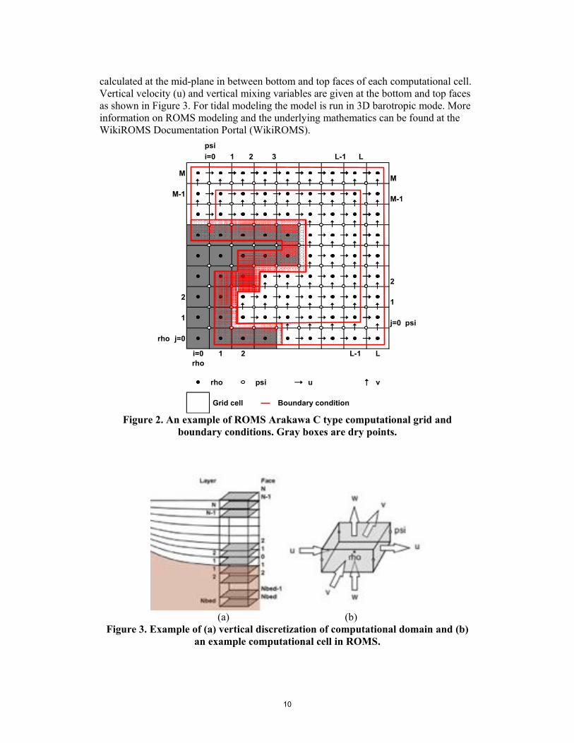
The computational grids are generated using the SeaGrid toolbox developed for Matlab to prepare an orthogonal grid within a curved perimeter suitable for oceanographic modeling (Denham 2008)The bathymetric data which is measured positive downwards from the MSL is used to generate depths for each grid point Grid points within the computational domain which remain permanently ldquodryrdquo are determined by masking the land cells using the coastline data The boundary between land and water is a solid wall boundary with free slip condition An example of ROMS Arakawa C type computational grid and boundary conditions are given in Figure 2 The scalar values such as density tracers and free surface are calculated at rho points located at the center of the computational cells The horizontal velocities (u and v) are computed on staggered grids that correspond to the interface of the computational cells The derivatives are calculated at psi points Therefore for a rectangular grid of M+1 by L+1 dimensions u v and psi has dimensions of M+1 by L M by L+1 and M by L respectively
ROMS uses a stretched terrain-following vertical coordinate system to conform to variable topography Therefore each vertical layer may have a different thickness The total height of the computational grid in the vertical is N+Nbed layers (Figure 2) In the present study sediment transport is not considered and therefore there is only one bed layer (Nbed=1) and it is fixed However the free-surface evolves in time The vertical discretization is also staggered so that the variables in the horizontal plane are
9
10
calculated at the mid-plane in between bottom and top faces of each computational cell Vertical velocity (u) and vertical mixing variables are given at the bottom and top faces as shown in Figure 3 For tidal modeling the model is run in 3D barotropic mode More information on ROMS modeling and the underlying mathematics can be found at the WikiROMS Documentation Portal (WikiROMS)
psi
i=0 1 2 3 L-1 L
M M
M-1 M-1
2
2 1
1 j=0 psi
rho j=0
i=0 1 2 L-1 L rho
rho psi u v
Grid cell Boundary condition
Figure 2 An example of ROMS Arakawa C type computational grid and boundary conditions Gray boxes are dry points
(a) (b)
Figure 3 Example of (a) vertical discretization of computational domain and (b) an example computational cell in ROMS
313 Grid Generation
In order to simulate the tidal flows inside the estuaries rivers inlets and bays more accurately numerical grid resolution needs to be kept small enough to resolve these features For this reason the USA coast is broken up into subgrids for separate simulations while keeping the computational domain at a manageable size Wherever possible natural barriers will be selected as boundaries between the different grids estuaries or bays are contained in their entirety within a single computational domain The neighboring grids contain overlaps of several kilometers to ensure seamless coverage
The United States coastline was divided into 52 subdomains with an average grid spacing of 350 m as shown in Figure 4 The only exception was the Puget Sound grid for which the results from an earlier study were used (Sutherland et al) The coastline data used for masking the land nodes was obtained from National Ocean Service (NOS) Medium Resolution Coastline via the Coastline Extractor (NGDC 2008a) and processed in MATLAB to remove the gaps Raw bathymetry was obtained from NOS Hydrographic Surveys Database (NOS 2008a) The bathymetry data from the database are generally referenced to mean low low water (MLLW) while ROMS bathymetry is defined with respect to mean water level (MWL) or mean tidal level (MTL) A conversion from MLLW to MTL referenced values was performed based on the data from the present Epochrsquos datum data provided by National Oceanic and Atmospheric Administration (NOAA) Tides amp Currents at the tidal stations (NOAA 2008b) or NOAA Vertical Datum Transformation software (VDatum) (NOS 2008b) Supplementary data to replace missing bathymetry points were acquired from NOAA Electronic Navigational Charts (NOAA 2008a) and National Geophysical Data Center Geophysical Data System database (GEODAS) (NGDC)
The bathymetric data is interpolated onto the model grid Even with the relatively high resolution of the grid (~350 m) the spatial variability of the bathymetry is not always fully resolved As pointed out in the validation report (Steward and Neary 2011) the bathymetric difference between the model and ADCP measurements are sometimes observed to be as large as 30 This may be a result of bathymetric variations on spatial scales shorter than the grid scale For a more detailed site characterization study higher spatial resolution for the model would alleviate these differences
11
Figure 4 Map of computational grids and the calibration data sources Harmonic constituents for tidal currents (green) and water levels (black) and prediction for
maximum current (yellow) and highlow tide elevations (purple)
12
The additional volume of water provided by the wetlands was implemented in the computational model through the wet-dry module in ROMS which allows for computational nodes to be defined as land or sea nodes dynamically with respect to the water content Wetland boundaries were acquired from National Wetland Inventory of US Fish amp Wildlife Services (USFWS) Elevation data for wetlands is cropped from the 1 arc second topography data downloaded from USGS Seamless Server (USGS) The topography data is referred to NAVD88 The data is converted to MTL reference via interpolating from NOAA tidal stations datum in the model domain or VDatum where available After conversion the sea bathymetry and the wetland topography are merged into a single set of points before constructing the computational grids A quadratic bottom stress formulation with a spatially uniform friction factor is used for each grid
Tidal constituents are periodic oscillations driven by the celestial forces computed with the mathematical approximation of the astronomical tides is given as
ே (2) ሻȉ ݐ ߜ ȉ ሺߪ ୀଵσ ܪ ൌ where H is the astronomical tide at time t since the start of the tidal epoch a0 is the vertical offset ai Vi Gi are the amplitude angular frequency and phase angle of the ith
tidal constituent (Zevenbergen et al 2004) For the US East coast and the Gulf of Mexico the ROMS tidal forcing file was generated by interpolating the ADCIRC (ADCIRC) tidal database at the open boundary nodes of the ROMS grid The harmonic constituents used for the forcing included Q1 O1 K1 S2 M2 N2 K2 M4 and M6 For the West coast and Alaska domains TPXO data (ESR) with the constituents Q1 O1 K1 S2 M2 N2 and M4 is used The M6 constituent is not included in the TPXO data and therefore cannot be included in the forcing For this dataset it was also found that more accurate results for S2 were obtained when not including K2 because they have such similar frequencies it is difficult to separate them for 30 day simulations
Stream flow data is obtained from USGS National Water Information System (USGS 2008b) when needed and yearly average discharges are applied as a point source at the major river boundaries Open boundary conditions were defined identically in all of the grids as free-surface Chapman condition (Chapman 1985) for the tidal elevation Flather condition (Carter and Merrifield 2007) for barotropic velocity (2D momentum) and gradient (aka Neumann) condition for baroclinic velocity (3D momentum) (WikiROMS) The results from 30-day simulations were used in the analyses after running the model for 32-day simulations with 2 days for the spin-up
32 Model calibration
The calibration data includes the in-situ measurements collected from various sources harmonic constituents and as well as the highlow tide or maximumminimum current predictions from NOAA Tides amp Currents If measurements with duration longer than a month are available harmonic constituents are extracted from both model and data to be compared For the calibration data that contain only highlow tides or maximumminimum currents the extreme values are extracted from the model for calibration Harmonic constituent calibrations are preferred over extreme value calibrations since the harmonic constituents are obtained from measurement sites and
13
may be more reliable than the predicted extreme values Therefore extreme value calibrations are only used when there are few or no measurements sites in the region
The calibration procedure begins with a full 32 day model run which is then compared with the data Due to the quantity and size of the different domains used in this study a holistic approach about the general trend of over versus under predictions for the constituents at all the various stations in the domain was used to develop a target overall relative error in currents To achieve the necessary relative change in currents the friction factor was modified uniformly for the entire grid and a shorter model run consisting of 7 days was completed In general a larger friction factor produces more drag thereby decreasing the currents For a more localized study a more quantitative approach may be utilized with spatially varying friction factors along with tuning of other model parameters such as turbulence parameters For the shorter model runs the relative changes in time series of the magnitude of the currents were evaluated and this process was repeated until the desired relative change was obtained Finally another 32 day model run was completed with the selected parameter values for the creation of the final harmonic constituents
The calibration parameters regarding the harmonic constituents of tidal elevations harmonic constituents of tidal currents and predicted maximumminimum tidal currents and predicted highlow tides are explained below
321 Harmonic Constituents for Tidal Currents
Amplitude Difference (amd)
This parameter shows how much the model underpredicts (amd lt 0) or overpredicts (amd gt 0) the amplitude of the kth harmonic constituent
୩ൌሺ୫ሻ୩െሺ୶ሻ୩ (3) where ሺ୫ሻ୩and ሺ୶ሻ୩ are the combined amplitudes of the kth harmonic constituent computed by the model output and given in data respectively The combined amplitude for each harmonic constituent is calculated as the square root of the squares of major and minor axes of the tidal ellipse
ൌ ට୫ୟ୨ଶ ୫୧୬ଶ (4)
where ୫ୟ୨ and ୫୧୬ are the major and the minor axis amplitudes of the tidal ellipse
Percentage Amplitude Difference (amdp)
A dimensionless parameter that gives the percent underprediction (amdp lt 0) or overprediction (amdp gt 0) of the amplitude of the kth harmonic constituent
୩ൌሺୟ୫୮ሻౡሺୟ୫୮౮ሻౡ ȉ ͳͲͲ (5)ሺୟ୫୮౮ሻౡ
14
Tidal Ellipse Inclination Difference (incd)
The difference between the inclination of the tidal ellipses (plusmn180 degrees) calculated by the model and given with the measurements
୩ ൌሺ୫ሻ୩െሺ୶ሻ୩ (6) where ሺ୫ሻ୩ and ሺ୶ሻ୩ are the orientation of the tidal ellipse (measured in degrees clockwise from North) of the kth harmonic constituent computed by the model output and given in data respectively
Phase Difference (phd)
This parameter indicates how much the model output lags (phd gt 0) or leads (phd lt 0) the given data for each of the modeled harmonic constituent for water surface level
୩ ൌሺ୫ሻ୩െሺ୶ሻ୩ (7) where ሺ୫ሻ୩ and ሺ୶ሻ୩ are the phases of the kth harmonic constituent computed by the model output and given in data respectively in minutes
322 Harmonic Constituents for Water Level
The calibration parameters for the harmonic constituents for water levels include amplitude difference (amd) percentage amplitude difference (amdp) and phase difference (phd) and are defined in the same manner with the calibration parameters for the harmonic constituents for tidal currents
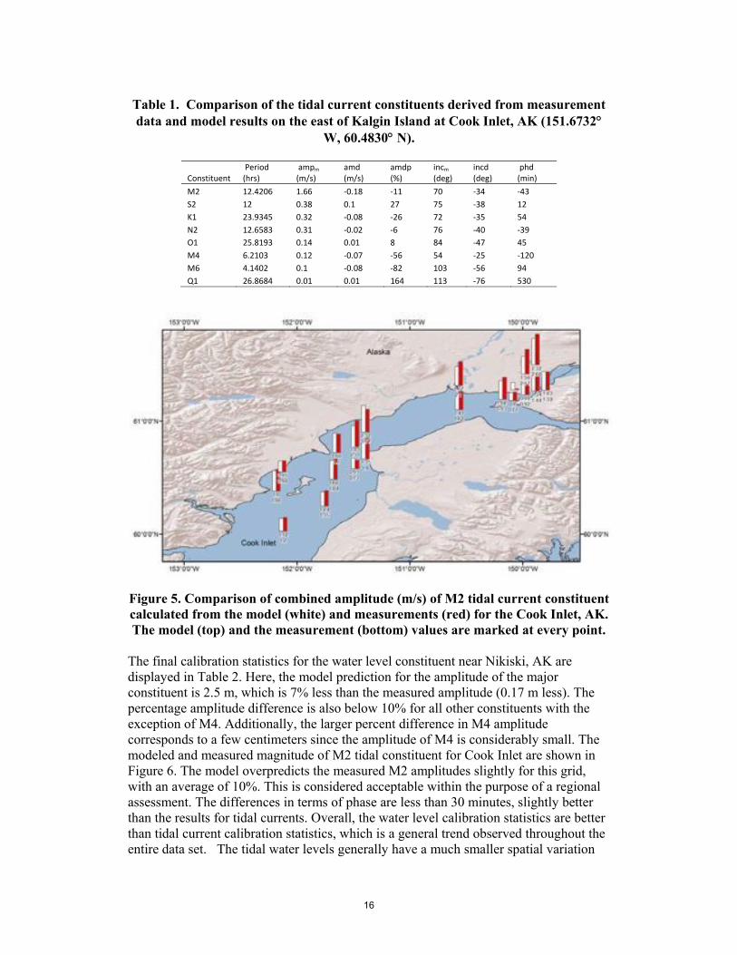
Statistics of final results from two points at Cook Inlet after calibration are given here as an example The comparison of the tidal current constituents derived from measurement data and model results on the east of Kalgin Island is shown in Table 1 According to the model the combined amplitude (ampm) for major constituent M2 at this location is 166 ms which is 11 less than the combined amplitude derived from the measurements (018 ms smaller) The percentage amplitude difference is larger for S2 and K1 than M2 although they translate to a much smaller amplitude difference between the measurements and the model results The calibration process involves overall evaluation of results from every measurement point in a given computational grid The results for combined magnitude of M2 tidal current constituent for Cook Inlet AK are shown in Figure 5 It is seen that the model can be overpredicting or underpredicting given that the results are within an acceptable range The average absolute difference between the model and the measurements in Cook Inlet for the combined amplitude and the tidal ellipse inclination are 19 and 13 respectively The phase differences are found to be under an hour for the first five major constituents which is reasonable since the model output is recorded hourly It is also seen that as the amplitude of the constituent starts to diminish the error in phase can increase significantly (eg 530 minutes for Q1) However this does not impose a major problem when the amplitude is negligible
15
Table 1 Comparison of the tidal current constituents derived from measurement data and model results on the east of Kalgin Island at Cook Inlet AK (1516732q
W 604830q N)
Period ampm amd amdp incm incd phd Constituent (hrs) (ms) (ms) () (deg) (deg) (min) M2 124206 166 Ͳ018 Ͳ11 70 Ͳ34 Ͳ43 S2 12 038 01 27 75 Ͳ38 12 K1 239345 032 Ͳ008 Ͳ26 72 Ͳ35 54 N2 126583 031 Ͳ002 Ͳ6 76 Ͳ40 Ͳ39 O1 258193 014 001 8 84 Ͳ47 45 M4 62103 012 Ͳ007 Ͳ56 54 Ͳ25 Ͳ120 M6 41402 01 Ͳ008 Ͳ82 103 Ͳ56 94 Q1 268684 001 001 164 113 Ͳ76 530
Figure 5 Comparison of combined amplitude (ms) of M2 tidal current constituent calculated from the model (white) and measurements (red) for the Cook Inlet AK The model (top) and the measurement (bottom) values are marked at every point
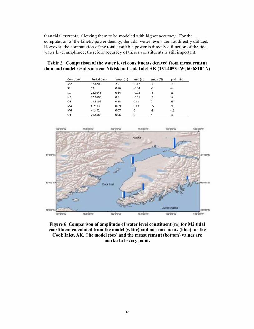
The final calibration statistics for the water level constituent near Nikiski AK are displayed in Table 2 Here the model prediction for the amplitude of the major constituent is 25 m which is 7 less than the measured amplitude (017 m less) The percentage amplitude difference is also below 10 for all other constituents with the exception of M4 Additionally the larger percent difference in M4 amplitude corresponds to a few centimeters since the amplitude of M4 is considerably small The modeled and measured magnitude of M2 tidal constituent for Cook Inlet are shown in Figure 6 The model overpredicts the measured M2 amplitudes slightly for this grid with an average of 10 This is considered acceptable within the purpose of a regional assessment The differences in terms of phase are less than 30 minutes slightly better than the results for tidal currents Overall the water level calibration statistics are better than tidal current calibration statistics which is a general trend observed throughout the entire data set The tidal water levels generally have a much smaller spatial variation
16
than tidal currents allowing them to be modeled with higher accuracy For the computation of the kinetic power density the tidal water levels are not directly utilized However the computation of the total available power is directly a function of the tidal water level amplitude therefore accuracy of theses constituents is still important
Table 2 Comparison of the water level constituents derived from measurement data and model results at near Nikiski at Cook Inlet AK (1514053q W 606810q N)
Constituent Period (hrs) ampm (m) amd (m) amdp () phd (min) M2 124206 25 Ͳ017 Ͳ7 Ͳ25 S2 12 086 Ͳ004 Ͳ5 Ͳ4 K1 239345 064 Ͳ005 Ͳ8 11 N2 126583 05 Ͳ001 Ͳ2 Ͳ6 O1 258193 038 001 2 25 M4 62103 009 003 35 Ͳ9 M6 41402 007 0 Ͳ2 Ͳ12 Q1 268684 006 0 4 Ͳ8
Figure 6 Comparison of amplitude of water level constituent (m) for M2 tidal constituent calculated from the model (white) and measurements (blue) for the
Cook Inlet AK The model (top) and the measurement (bottom) values are marked at every point
17
323 Predicted Maximum Currents
Mean current magnitude ratio of maximum currents (cmgrt)
The average ratio of the maximum current magnitudes from the model to the magnitudes of the corresponding maximum current values from the calibration data are given by
หሺೠሻหσ หሺೠሻห (8) సభൌݐݎ ே
where curm is the maximum current magnitude from the model and curv is the maximum current value from the calibration data i and N are the ith occurrence and total number of occurrences of maximum and minimum during the simulation duration respectively
Root-mean-square difference of maximum currents (crms fcrms ecrm)
This parameter is the root-mean-square of the difference between the maximum current values output by the model and maximum current values from the data and is an estimate for the error in predicting maximum current magnitude
(9)
మሽሻೡ௨ሺሻ௨ሼሺసభσටൌݏݎ ேCurrent root-mean-square differences for maximum flood and ebb currents (fcrms and ecrms) are calculated using the same equation but only the maximum of the flood (or ebb) tides are used to compare
Mean difference in maximum flood (or ebb) currents (fcmd and ecmd)
The mean difference in maximum flood current between the model output and the calibration data shows whether the model produced larger flood current (fcmd gt 0) or smaller flood current (fcmd lt 0) than the calibration data It is given by
ቁ ቁσసభቄቀ௨ ቀ௨ೡ ቅ(10)
ேൌare maximum flood currents from the model and from data ௩ݎݑand
ݎݑwhere respectively Similarly the difference in maximum ebb current between the model output and the calibration data is computed by
సభ ሻሺ௨ೡሻሽ ሼሺ௨ (11) σൌ ே௩ݎݑ and are maximum flood currents from the model and from data ݎݑwhere
respectively fcmd and ecmd are used to evaluate ability of the model to simulate the flood or ebb dominant tidal regimes
Phase Difference between Maximum Currents (cpd fcpd and ecpd)
The mean phase difference for maximum currents and the mean phase difference for maximum flood and ebb currents are given by
ሼሺ௧ሻሺ௧ೡሻሽసభ (12) σൌ ே
18
ൌ ቁ ቁσసభቄቀ௧
ቀ௧ೡ ቅ
(13)ே ሼሺ௧ (14)ሽሻೡ௧ሺሻసభσൌ ே
where tm and tv are the times that correspond to the maximum tidal current occurrences in the model output and the calibration data respectively The superscripts f and e denote flood and ebb Current phase difference is an estimate of how much the model phase lags (cpd fcpd ecpd gt 0) or precedes (cpd fcpd ecpd lt 0) the calibration data
324 Predicted HighLow Tides
Standard Deviation Ratio of HighLow Tides (stdrt)
The ratio between standard deviation of the highlow tide computed with the model and given in the data It is an estimate of how much the model underpredicts (stdrt lt 1) or overpredicts (stdrt gt 1) the tidal range
തതതതതതതതൟమඨσ ൛ሺ౬ሻష౬సభ
ൌ (15)
തതതതതതതൟమඨσ ൛ሺ౬౬ሻష౬౬సభ
where elvm and elvv are the highlow tide time series from the model and the data
Root-Mean-Square Difference of HighLow Tides (rms hirms and lorms)
The root mean square difference between the model output and the data for highlow tides is an estimate for the error of the model prediction in predicting the tidal elevation It is given by
సభሼሺ୪୴ሻሺ୪୴౬ሻሽమൌ ටσ (16)
Phase Difference between HighLow Tide (phd hiphd and lophd)
These terms show the phase difference between the NOAA predictions and the model for highlow tides regarding only high tides only (hiphd) or low itdes only (lophd) or both (phd) They measure how much the model output lags (phd hiphd lophd gt 0) or leads (phd hiphd lophd lt 0) the change in the water surface level It is calculated with the same equations for currents by substituting the high and low tide times into the equation
Calibration statistics of model results with NOAA predictions for maximum currents is demonstrated with examples from St Catherines Sound in Georgia in Table 3 This location has moderate tidal currents with average magnitude for maximum currents (cmgm) less than 1 ms It is seen that the model usually overpredicts the magnitude of maximum tidal current for this particular location However the data shown here covers only a small part of the computational grid that includes several sounds for which the results also include underpredictions For this specific example depending on the location the mean current magnitude ratio (cmgrt) can be as high as 132 although
19
much higher values are common for the complete set of data The large differences for the maximum current predictions can be attributed to many reasons In addition to correct prediction of the currents being more challenging than water levels comparing the results with predictions rather than directly to measurements introduces some ambiguity Having only the maximum predicted values to compare against can contribute to larger differences On the other hand although the magnitude differences can vary largely the phase differences for the maximum current speed are generally on the order of an hour for the entire data set For the locations considered in the St Catherines Sound the time differences are calculated to be slightly larger than half an hour
Table 3 Maximum current predictions at St Catherines Sound and Newport River GA
Longitude Latitude cmgm cmgrt crms cpd Station Name (deg) (deg) (ms) (Ͳ) (ms) (min)
St Catherines Sound Entrance Ͳ811405 317150 094 132 039 33
Medway River northwest of Cedar Point Ͳ811908 317145 082 136 044 Ͳ52
N Newport River NE of Vandyke Creek Ͳ811870 316912 082 129 042 52
N Newport River above Walburg Creek Ͳ811953 316738 075 100 025 Ͳ49
N Newport River NW of Johnson Creek Ͳ812105 316630 074 117 032 Ͳ23
N Newport River ESE of S Newport Cut Ͳ812645 316653 064 141 035 10
The tidal range in St Catherine Sound GA is predicted to be slightly larger than 2 m based on the highlow water calibrations statistics of the locations displayed in Table 4 The root-mean-square difference in highlow tides is approximately 014 ms which is satisfactory for the given tidal range The standard deviation ratio of highlow water levels (stdrt) is slightly less than 1 at all of the locations indicating that the modeled tidal range is slightly smaller than the NOAA predictions The modeled highlow tides are found to lead the predictions nearly by half an hour
Table 4 Highlow water elevation predictions at St Catherines Sound and Newport River GA
Mean of Mean of Longitude Latitude High Low Water rms phd
Station Name (deg) (deg) Water (m) (m) strdt (Ͳ) (m) (min)
Walburg Creek entrance Ͳ813667 315500 110 Ͳ097 093 015 Ͳ28
Bear River Entrance Ͳ813167 314833 110 Ͳ095 092 016 Ͳ27
North Newport River Ͳ814667 313333 120 Ͳ101 095 013 Ͳ32
South Newport Cut N Newport River Ͳ814000 313000 115 Ͳ102 097 011 Ͳ43
Like the maximum current predictions highlow water predictions are also based on numerical modeling The predictions are less reliable sources than the actual measurements and are only used for calibration when there is no measured data available Nevertheless when both sources are available the final calibration statistics for them are published together with the measurement data even if they are not used in calibration
20
33 Validation of model results
An independent validation of the model performance in predicting tidal elevation and depth-averaged velocity was done by the Oak Ridge National Laboratory (ORNL) at locations where true values were taken as point measurements from tidal monitoring stations (Stewart and Neary 2011) Two classes of point measurements were defined for the purpose of validation Class 1 validation is a split sample validation commonly used to evaluate the performance of a calibrated model with measurements independent of those used for calibration whereas Class 2 validation is an assessment of the model calibration procedure using different performance metrics (Stewart and Neary 2011) than those described here More than fifty measurement stations are selected for validation based on 1) Various levels of power densities 2) Vicinity to larger population and cities and 3) Representative of several different areas along the US Correlation statistics including phase shift amplitude ratio and coefficient of determination (R2) value are calculated along with model performance metrics that include the root mean square error Nash-Sutcliffe efficiency coefficient and mean absolute error Predicted and measured depth-averaged current speed frequency and cumulative frequency histograms means standard deviation and maximum and minimum value are compared Further information about the validation procedure and detailed results is available in the original source (Stewart and Neary 2011)
Following the EMEC guidelines for a regional assessment model predictions are considered adequate when predicted maximum current speeds are within 30 of those estimated from tidal monitoring station measurements The validation results indicate a fair model performance for predicting currents speeds and tidal elevation with R2 values ranging values ranging from 076 to 080 and from 079 to 085 respectively The model has a slight tendency to over predict mean and max current speeds for medium to high power density regions and a tendency to under predict speeds in low power density regions Based on the comparison of measured and predicted current speeds for both classes of stations located in the medium to high power density regions the model over predicts mean and maximum current speeds by 24 and 21 on average respectively Similarly for those stations that are under predicted it is done so by -18 on average for the mean current speeds and -13 on average for the max current speed The model performance for the prediction of tidal elevations is found to be better than the tidal currents
The validation methodology focuses on comparing the time-series of the current speeds and elevations as opposed to comparing tidal constituents The time series for model are constructed from the final constituent database and compared to the measured time series Hence any effects related to wind driven flow and fresh water intrusion and even localized effects caused by flooding in tidal rivers can influence the validation results In addition the validation procedure recognizes the limitations of regional assessment models with coarse grid resolution to predict local variations in current speed and tidal elevation within 300 m to 500 m parcels Model performance evaluations are therefore restricted because model predicted values that are spatially averaged over a 300 m to 500 m grid cell cannot be expected to correspond with tidal monitoring station measurements taken at a point at a given latitude and longitude Tidal currents at places like Admiralty Inlet have been shown to vary greatly over scales less than 500 m (Epler
21
2010) Overall the model predictions are found to be satisfactory for purposes of regional assessment of tidal stream power potential
34 Assessment of tidal stream resource The tidal database includes the harmonic constituents for both the water level and the depth-averaged currents These constituents may be used to compute time series of the currents for any time period and to find the kinetic power density (kWm2) This is the theoretical available kinetic power density for a particular location which does not include any assumptions about technology nor does it account for any flow field effects from energy extraction
At the request of DOE we have also estimated the total theoretical available power which has units of power (ie gigawatts) This needs to be estimated on the scale of individual estuaries and involves the total power and not just the kinetic power of the tides This estimate also requires incorporating the cumulative effects of energy dissipation to determine the maximum amount of energy which may be dissipated However this estimate also does not involve assumptions about particular technologies
341 Theoretical available kinetic power density
The tidal stream power is evaluated by computing the kinetic power density from the tidal current speeds using
(17)ଷ ȉ ߩ ȉ ଵ ൌ ଶwhere P is the tidal stream power per unit area of flow ie tidal stream power density U is the density of seawater and V is the current speed Because of the desire towards the use of open turbines rather than tidal barrages and the fact that existing tidal stream power conversion technologies have minimum current speed requirements for power take-off there is a tendency for the identification of hotspots based on the kinetic power of the tides rather than their tidal head Stronger tidal streams mean faster currents which corresponds to a cubical increase in power density The overall power that can be converted from tidal streams is a function of both the kinetic and potential energy with other parameters such as the site characteristics device characteristics and environmental impacts also influencing the calculation of the practical resource potential (defined as the amount of power which can actually be extracted under all such constraints) Calculating the practical resource of a hotspot will require much more detailed site characterization
On the other hand a regional assessment is well suited for the purpose of site screening Additionally minimum current speed and minimum depth requirements can be imposed in order to narrow down the number of hotspots Generally tidal stream power converters require a minimum flow speed (cut-in speed) to start operating which ranges from 05 ms to 1 ms depending on their design Although some studies that simulate power extraction acknowledge cut-in speed values for the horizontal axis turbines as large as 1 ms (Lim and Koh 2010 Myers and Bahaj 2005) there are many examples with cut-in speeds around 07 ms and a vertical axis turbine with 05 ms (Bedard et al 2006 Fraenkel 2007 Lee et al 2009) In this study the minimum for the power density is selected as 500 Wm2 which corresponds to a flow speed of ~1 ms If the
22
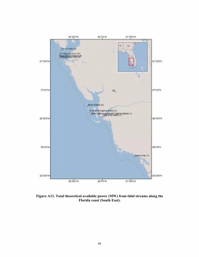
maximum of the mean kinetic power does not exceed 500 Wm2 within the boundaries of the hotspot area the hotspot is excluded from the list Regardless of their design the tidal stream power converters also require a minimum depth that allows for allocating the device with enough top and bottom clearance The dimensions of tidal stream power devices change from several meters to tens of meters (Bedard et al 2006 Froberg 2006) and since the analysis in this study does not depend on a specific device the minimum depth is chosen to be 5 m large enough to accommodate a small size conversion device with the existing technology Finally the list of hotspots is filtered with a minimum surface area requirement of 05 km2 The surface area does not contribute to power density is expected to accommodate larger space for development This final filter also reduces the number hotspots to a two-page list by removing more than two thirds of the initial list Based on these criteria the geospatial data along the USA coast has been filtered to define the hotspots with notable tidal stream power densities which are listed in Table 5 The coordinates of each hotspot location maximum and average depth with respect to Mean Lower Low Water (MLLW) and surface area of these regions are given together with the largest mean power density within each location For brevity the listed locations mark the general vicinity of the hotspots and do not necessarily pinpoint the exact location of each hotspot individually For further analysis the reader is suggested to visit the original geodatabase (GT 2011)
Table 5 Locations and characteristics of the theoretical available tidal stream density hotspots along the coast of USA
State Hotspot Location Surface Maximum Mean Kinetic Power (degrees N degrees W) Area Depth Depth Density
(sqkm) (m) (m) (Wsqm)
ME Coobscook Bay (44891 67107) lt 1 17 14 574 ME Lubec Channel (44853 66977) lt 1 8 7 891 ME Grand Manan Channel (448 66892) 21 101 79 768 ME Western Paasage (44911 66977) 7 106 43 7366 ME Knubble bay (43882 69731) lt 1 14 11 730 ME Hockmock Bay (43902 69737) (43912 69718) lt 1 lt 1 12 7 7 6 1747 567 ME Kennebeck River (4393 6981) (43969 69825) lt 1 lt 1 7 8 7 8 552 528 MENH Piscataqua River (43073 70728) (43092 70775) 2 1 20 17 13 12 2823 2633
(43113 70807) lt 1 13 9 1239 MA Nantucket Sound (41197 69902) (41345 70396) 398 38 39 16 10 7328 4844
202 MA Vineyard Sound (41499 70647) (41362 70854) 137 2 33 24 19 15 3344 603 NY Block Island Sound (41229 72061) (41167 7221) 7 2 85 49 38 21 740 610
(41075 71845) 4 15 12 530 NY East Rive (4079 73935) (40775 73937) lt 1 lt 5 1 5 6 547 1546
(40706 73979) 1 11 11 768 lt 1
NJ Delaware Bay (38921 74963) 11 13 9 913 NC Cape Hatteras (35185 75762) lt 1 9 8 1378 NC Portsmouth Island (35068 76016) 3 10 7 911 SC Cooper River (3288 79961) lt 1 8 7 830 SC North Edisto River (32576 802) 7 19 12 1008 SC Coosaw River (32492 8049) 12 17 10 566 GA Ogeechee River (31856 81118) 1 8 7 834 GA Altamaha River (31319 81309) 1 8 6 511 GA Satilla River (3097 81505) lt 1 8 7 606 GAFL St Marys River (30707 81445) (30721 81508) 5 lt 1 20 8 12 6 798 705 FL Florida Keys (24692 81143) (24681 81168) 3 1 10 7 6 6 992643
(24574 81839) (24556 82056) 10 29 11 10 7 6 904 538
23
24
FL Port Boca Grande (26716 82251) lt 1 20 10 1140 FL St Vincrnt island (29625 85101) lt 1 11 8 625 CA Golden Gate (37822 122471) lt 1 111 50 750 CA Carquinez Strait (38036 122158) 12 36 19 914 CA Humbolt Bay Entrance (40757 124231) lt 1 11 9 941 OR Coos Bay Entrance (43353 124339) 1 13 8 2480 WA Columbia River (46254 124026) (46253 123563) 35 2 14 11 11 10 1751 689 WA Grays Harbor (46917 124117) 11 9 8 576 WA Haro Strait (48495 123154) (48587 123218) 15 15 276 271 232 199 625 503 WA Spieden Channel (4863 123126) 5 60 43 1893 WA President Channel (48656 123139) (48679 122999) 4 4 54 155 39 129 1227 528 WA San Juan Channel (48547 122978) 7 93 62 1030 WA Middle Channel (48459 122949) 8 93 60 2380 WA Boundary Pass (48735 123061) 8 308 163 620 WA Rosario Strait (48594 122755) 45 92 53 3349 WA Bellingham Channel (48556 122658) 17 45 27 3077 WA Guemes Channel (48523 122621) 2 8 7 1777 WA Deception Pass (48407 122627) 2 6 6 1058 WA Admiralty Inlet (48162 122737) 54 141 62 907 WA Puget Sound (47591 122559) 2 22 11 2568 WA Tacoma Narrows (47268 122544) 13 64 39 5602 WA Dana Paasage (47164 122862) 3 18 13 1851 AK Bristol Bay (58604 162268) (58532 160923) 160 48 13 28 11 5000 654
(58442 158693) 11 199 12 957 304
AK Nushagak Bay (58975 158519) 122 14 8 2811 AK Hague Channel (55908 160574) 1 24 17 564 AK Herendeen Bay Entrance (55892 160793) 10 38 19 1564 AK Moffet Lagoon Inlet (55446 162587) 1 7 7 845 AK Izembek Lagoon (55328 162896) (55248 162981) lt 1 1 8 6 7 6 539 1606 AK Bechevin Bay (55048 16345) 4 7 6 2252 AK False Pass (54827 163384) 5 60 35 1619 AK Unimak Pass (54333 164824) 132 82 57 830 AK Ugamak Strait (54168 164914) 63 88 48 1341 AK Derbin Strait (54092 165235) 23 97 54 2348 AK Avatanak Strait (54108 165478) 73 136 73 911 AK Akutan Bay (54129 165649) 4 44 26 3365 AK Akutan Pass (54025 166074) 50 83 49 2870 AK Unalga Pass (53948 16621) 25 117 64 3751 AK Umnk Pass (53322 167893) 97 138 56 2144 AK Samalga Pass (52808 169122) (52765 169346) 8 138 30 277 13 103 4102 1718
(52757 169686) 66 195 140 794 AK Islands of Four Mountains (52862 169998) 7 147 53 2505 AK Seguam Pass (52247 172673) (52132 172826) 52 128 190 151 129 85 800 538 AK Atka Island (52121 174065) 41 70 36 3444 AK Fenimore Pass (51998 175388) (51979 175477) 4 28 95 30 52 16 2147 1554 AK Fenimore Pass (51974 175532) (51961 175649) 3 1 97 25 50 20 2410 1304 AK Chugul Island (51937 175755) (51961 175866) 9 9 100 81 47 48 1677 1600 AK Igitkin Island (51968 175974) 9 93 59 1110 AK Unmak Island (51857 176066) 1 26 22 1155 AK Little Tanaga Strait (51818 176254) 6 68 43 2276 AK Kagalaska Strait (5179 176414) 1 20 18 758 AK Adak Strait (51816 176982) 63 93 63 807 AK Kanaga Pass (51723 177748) 36 55 29 889 AK Delar of Islands (51677 17819) (5155 178467) 83 54 217 102 78 64 764 649
(51564 178716) (51586 178928) 8 31 19 126 11 66 537 1053
AK Chirikof island (55964 15545) 198 44 31 597 AK Tugidak Island (56294 154872) 284 51 26 681 AK Sitkinak Island (56512 154383) 13 40 8 3104
AK Aiaktalik Island (56639 154072) (56738 154053) 79 23 69 33 28 16 2497 2038 AK Moser Bay (57038 154115) 3 10 7 1874 AK Kopreanof Strait (57934 15284) (57987 152795) 17 10 59 21 29 14 5454 4636 AK Shuyak Strait (58466 152496) 2 23 15 1007 AK Stevenson Entrance (58647 152292) (58663 152525) 33 7 157 75 102 39 895 779 AK Barren Islands (58939 152127) (58855 152345) 15 9 115 127 73 78 686 571 AK Chugach Island (59091 151777) (5912 151875) 34 19 116 96 54 64 587 528
(59148 15174) (59163 151531) 15 13 90 58 26 34 1466 916 (59082 151433) 20 64 47 852
AK Cook Inlet (60676 15158) 5285 140 34 5344 AK Turnagain Arm (60978 149825) (60982 149702) 8 5 13 6 9 5 3199 657
(60998 149729) 2 5 5 558 AK Knik Arm (61385 149809) (61396 14977) 42 6 5 6 5 1993 742
(6141 149734) (61428 149709) 2 3 5 7 5 6 749 597 (61371 149726) 3 6 6 1048
AK Shelikof Strait (58239 151752) 15 31 24 524 AK Montague Strait (59767 147966) 29 36 26 691 AK Icy Strait (58353 135994) 274 287 94 8781 AK Cross Sound (58223 136356) (58225 136302) 33 79 139 72 79 976 503
(58256 136372) (58288 135819) 1 9 55 124 46 84 945 513 AK Adams Inlet (58863 135979) 4 16 9 1426 AK Peril Strait (57455 135549) (57371 135695) 1 2 7 43 7 24 3285 892 AK Taku inlet (58384 134032) 4 14 10 864 AK Seymour Canal (57922 134156) (5793 134276) lt 1 lt 14 5 14 5 770 976
1 AK Summer Strait (56369 133658) (56437 13319) 11 6 185 45 67 15 1474 801
(56441 133028) 4 184 101 529 AK Duncan Canal (5654 133088) lt 1 37 37 604 AK Kashevarof Passage (56233 133043) (56269 132948) 6 7 37 109 27 80 1039 744 AK Meares Passage (55259 133109) 1 17 14 1692
The list of hotspots in table 5 shows that Alaska (AK) has the largest number of hotspots including some of the largest kinetic power density in the USA With a surface area that is an order of magnitude larger than the rest of the hotspots and a substantially large kinetic power density Cook Inlet is one of the best resources of tidal stream power The largest kinetic power density locations include Bristol Bay Akutan Unalga and Samalga Passes Sikitnak Island Turnagain Arm and Kopreanof Icy and Peril Straits Maine (ME) Washington (WA) Oregon (OR) California (CA) New Hampshire (NH) Massachusetts (MA) New York (NY) New Jersey (NJ) North and South Carolina (NC SC) Georgia (GA) and Florida (FL) follow Alaska Tacoma Narrows Rosario Strait Bellingham Channel Nantucket Sound and Western Passage are some of the hotspots with largest kinetic power density The list given with this study includes the top tier tidal stream power density hotspots at a national resource assessment scale based on numerical modeling of the tidal currents and after certain filtering There are many locations that are excluded as a result of applied filters however they can be found in the original geodatabase Some of the filtered locations with tidal power density greater than 250 Wm2 include but not limited to Cape Cod Canal in MA Hudson River in NY Great Egg Harbor Bay in NJ Cape Fear in NC Charleston Harbor Port Royal Sound Cooper and Beaufort Rivers in SC St Johns River in FL Carquinez Strait Eel and Siltcoos Rivers in CA Mud Bay Entrance and Cooper River Delta in AK There may also be additional locations that are viable for tidal stream power conversion but which are not resolved by the numerical model These are probably local resources that can only be detected through finer modeling at smaller scales or with field measurements such as the Kootznahoo Inlet in AK Willapa
25
Bay in WA Sheepscot Bay in ME Shelter Island Sound in NY Manasquan River in NJ
342 Total theoretical available power estimates
The published maps and the database provide the distribution of the existing kinetic power density of tidal streams in the undisturbed flow conditions These results do not include any technology assumptions or flow field effects as in the case of device arrays In order to calculate a theoretical upper bound based on physics only a simplified method that considers both the kinetic and potential power with the exclusion of any technology specific assumptions is applied The details of the method is outlined in a recent paper (Garrett and Cummins 2005) The power calculated with this method is used in estimating the tidal power potential for the entire country with a specific value for each state The method uses undisturbed flow field from the model with simple analytical methods accounts for the cumulative effect of dissipating energy and provides information on an estuary scale
Considering a constricted channel connecting two large bodies of water in which the tides at both ends are assumed to be unaffected by the currents through the channel a general formula gives the maximum average power as between 20 and 24 of the peak tidal pressure head times the peak of the undisturbed mass flux through the channel This maximum average power is independent of the location of the turbine fences along the channel Maximum average tidal stream power Pmax is given as
(18)௫ȉ ȉ ȉ ൌ ߛ ȉ ߩ ௫where J is a parameter U is the density of seawater a is the amplitude of the tidal water level constituent and Qmax is the maximum corresponding tidal flow rate For a background friction dominated nonsinusoidal (ie considering more than one tidal constituent) case if data for the head and flux in the natural state are available the maximum average power may be estimated with an accuracy of 10 using J = 022 without any need to understand the basic dynamical balance (Garrett and Cummins
)ǡ ǥଶଵA multiplying factor is used to account for additional constituents ( 2005) given as
ͳ ቀଽ ቁ ሺݎଵଶ ଶଶݎ ሻڮ (19)ଵమൌଶǡ where ݎభൌଵݎ ǥ
This upper bound on the available power ignores losses associated with turbine operation and assumes that turbines are deployed in uniform fences with all the water passing through the turbines at each fence
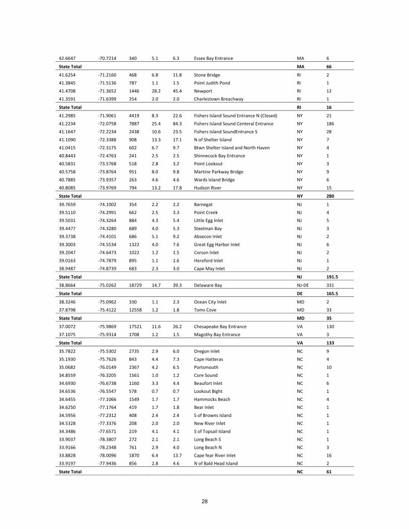
This method is applied to the locations bounded between two land masses and has locally increased tidal current speed along the United States coast A list of these locations grouped by state is given in Table 6 The list displays the coordinates and the name of each location (ie the midpoint) together with the width meanmaximum of the constriction and the total theoretical available power The totals are given for each state and for the entire country Once again Alaska with a total of 47GW constitutes the largest piece of the national total of 50 GW Cook Inlet has the largest average maximum available power of 18 GW (Figure A22) closely followed by Chatham Strait with 12 GW (Figure A20) Alaska is stands out as an abundant resource of tidal stream
26
power with eighty different promising locations The top ten of these locations include in addition to Cook Inlet and Chatham Strait north of Inian Islands (25 GW) in Figure A20 Summer Strait (27 GW) northeast of Warren Island (535 MW) Clarence Strait (41 GW) in Figure A19 between Sundstrom and Sitkinak Islands (628 MW) in Figure A21 between Seguam and Amlia Islands (12 GW) in Figure A26 Kagalaska and Adak Islands (424 MW) in Figure A28 and between Unalga and Kavalga Islands (435 MW) in Figure A29
On a state by state basis Alaska is followed by Washington and Maine with 683 and 675 MW respectively The other states with considerable average maximum power available from tidal streams include South Carolina (388 MW) New York (280 MW) Georgia (219 MW) California (204 MW) New Jersey (192 MW) Florida (166 MW) Delaware (165 MW) and Virginia (133MW) In addition Massachusetts (66 MW) North Carolina (66 MW) Oregon (48 MW) Maryland (35 MW) include other possible energetic locations with Rhode Island (16 MW) and Texas (6 MW) having somewhat limited overall tidal stream power Some of the sites with considerably larger power than their other alternatives in these states include Admiralty Inlet Entrance WA (456 MW) in Figure A18 east of Cross Island (269 MW) and south of Eastport ME (106 MW) in Figure A2 St Helena (102 MW) and Port Royal Sounds SC (109 MW) in Figure A9 Fisher Island Sound Entrance ( 186 MW) St Catherine (44 MW) and Sapelo Sounds GA (47 MW) in Figure A10 San Francisco Bay CA (178 MW) in Figure A17 Delaware Bay (331 MW) in Figure A5 Chesapeake Bay Entrance (130 MW) in Figure A6 and the Florida Keys in Figure A12
Table 6 Locations and characteristics of the total theoretical available power along the coast of USA
Mean Max Maximum Latitude Longitude Width depth depth Power (deg) (deg) (m) (m) (m) Name State (MW) 448889 Ͳ669908 1499 158 263 S of Eastport ME 106 449364 Ͳ670465 374 12 14 Bar Harbor ME 4 446198 Ͳ672786 765 65 76 N of Cross Island ME 26 445940 Ͳ675486 1362 66 153 NE of Roque Island ME 32 445915 Ͳ673949 943 40 73 Btwn Starboard and Foster Islands ME 21 445905 Ͳ673551 7008 291 566 E of Cross Island ME 269 445249 Ͳ676161 582 83 105 S of Jonesport ME 22 445148 Ͳ675655 813 36 55 Btwn Sheep and Head Harbor Islands ME 15 445688 Ͳ677583 628 28 31 Channel Rock ME 9 443851 Ͳ678845 2826 63 84 Btwn Southwest Breaker and Green Islands ME 68 441332 Ͳ683631 2036 105 151 Btwn East Sister and Crow Islands ME 61 442756 Ͳ686756 459 14 14 Deer Isle ME 3 445517 Ͳ688007 470 40 40 E of Verona Island ME 10 438503 Ͳ697152 627 173 198 NE of Mac Mahan Island ME 10 437909 Ͳ697857 619 125 128 N of Perkins Island ME 19 State Total ME 675 430730 Ͳ707075 656 127 180 New Castle MA 21 428198 Ͳ708176 428 63 65 Badgers Rock MA 11 426960 Ͳ707756 1049 29 50 Bass Rock MA 15 422997 Ͳ709245 525 91 120 Hull Gut MA 13
27
426647 Ͳ707214 340 51 63 Essex Bay Entrance MA 6 State Total MA 66 416254 Ͳ712160 468 68 118 Stone Bridge RI 2 413845 Ͳ715136 787 11 15 Point Judith Pond RI 1 414708 Ͳ713652 1446 282 454 Newport RI 12 413591 Ͳ716399 254 20 20 Charlestown Breachway RI 1 State Total RI 16 412985 Ͳ719061 4419 83 226 Fishers Island Sound Entrance N (Closed) NY 21 412234 Ͳ720758 7887 254 843 Fishers Island Sound Centeral Entrance NY 186 411647 Ͳ722234 2438 106 235 Fishers Island SoundEntrance S NY 28 411090 Ͳ723388 908 133 171 N of Shelter Island NY 7 410415 Ͳ723175 602 67 97 Btwn Shelter Island and North Haven NY 4 408443 Ͳ724763 241 25 25 Shinnecock Bay Entrance NY 1 405831 Ͳ735768 518 28 32 Point Lookout NY 3 405758 Ͳ738764 951 80 98 Martine Parkway Bridge NY 9 407885 Ͳ739357 263 46 46 Wards Island Bridge NY 6 408085 Ͳ739769 794 132 178 Hudson River NY 15 State Total NY 280 397659 Ͳ741002 354 22 22 Barnegat NJ 1 395110 Ͳ742991 662 25 33 Point Creek NJ 4 395031 Ͳ743264 884 43 54 Little Egg Inlet NJ 5 394477 Ͳ743280 689 40 53 Steelman Bay NJ 3 393738 Ͳ744101 686 51 92 Absecon Inlet NJ 2 393003 Ͳ745534 1322 40 76 Great Egg Harbor Inlet NJ 6 392047 Ͳ746473 1022 12 15 Corson Inlet NJ 2 390163 Ͳ747879 895 11 16 Hereford Inlet NJ 1 389487 Ͳ748739 683 23 30 Cape May Inlet NJ 2 State Total NJ 1915 388664 Ͳ750262 18729 147 393 Delaware Bay NJͲDE 331 State Total DE 1655 383246
378798
Ͳ750962 Ͳ754122
330 12558
11 12
23 18
Ocean City Inlet Toms Cove
MD MD
2 33
State Total MD 35 370072
371075
Ͳ759869 Ͳ759314
17521 1708
116 12
262 15
Chesapeake Bay Entrance Magothy Bay Entrance
VA VA
130 3
State Total VA 133 357822
351930
350682
348559
346930
346536
346455
346250
345956
345328
343486
339037
339166
338828
339197
Ͳ755302 Ͳ757626 Ͳ760149 Ͳ763205 Ͳ766738 Ͳ765547 Ͳ771066 Ͳ771764 Ͳ772312 Ͳ773376 Ͳ776571 Ͳ783807 Ͳ782348 Ͳ780096 Ͳ779436
2735 843 2367 1561 1160 578 1549 419 408 208 219 272 761 1870 856
29 44 42 10 33 07 17 17 24 20 41 21 29 64 28
60 73 65 12 44 07 17 18 24 20 41 21 40 137 46
Oregon Inlet Cape Hatteras Portsmouth Core Sound Beaufort Inlet Lookout Bight Hammocks Beach Bear Inlet S of Browns Island New River Inlet S of Topsail Island Long Beach S Long Beach N Cape fear River Inlet N of Bald Head Island
NC NC NC NC NC NC NC NC NC NC NC NC NC NC NC
9 4 10 1 6 1 4 1 1 1 1 1 3 16 2
State Total NC 61
28
29
330795 Ͳ793407 1591 23 28 Cape Romain Harbor SC 5 328808 Ͳ796555 535 28 31 Price Inlet SC 2 327535 Ͳ798683 1867 97 181 Charleston harbor SC 27 326896 Ͳ798895 265 16 16 Light House Inlet SC 1 325705 Ͳ801944 1022 87 172 S of Seabrook Island SC 22 324449 Ͳ803867 11818 57 116 Saint Helena Sound SC 102 323369 Ͳ804600 501 71 74 S of Hunting island SC 6 322491 Ͳ806599 3685 129 164 Port Royal Sound SC 109 321198 Ͳ808333 854 143 167 Calibogue Sound SC 25 320796 Ͳ808798 534 47 83 N of Turtle island SC 6 State Total SC 388 320354 Ͳ808882 483 97 125 N of Fort Pulski SC and GA 10 320205 Ͳ808884 481 44 49 S of Fort Pulaski GA 5 318682 Ͳ810688 1891 56 110 Btwn Green Island and Racoon Key GA 16 318478 Ͳ810792 1178 60 76 Btwn Racoon Key and Egg Islands GA 15 317117 Ͳ811388 2542 91 146 St Catherines Sound GA 44 315459 Ͳ811862 2734 79 148 Sapelo Sound GA 47 313185 Ͳ813057 929 47 65 Altamaha Sound GA 12 313075 Ͳ813254 754 12 20 Buttermilk Sound GA 3 310238 Ͳ814451 1694 47 67 Jekyll Sound GA 18 309681 Ͳ815017 1482 48 70 N of Pompey Island GA 18 307110 Ͳ814526 1132 116 182 Cumberland Sound Entrance GA and FL 31 State Total GA 219 305080 Ͳ814407 1548 40 79 Nassau Sound FL 10 304030 Ͳ814153 664 91 119 Fort George FL 10 299099 Ͳ812898 845 21 23 N of Anastasia State Park FL 4 298740 Ͳ812755 291 48 48 Anastasia State Park FL 2 297058 Ͳ812275 280 22 22 Matanzas Inlet FL 1 290744 Ͳ809204 635 20 24 Ponce Inlet FL 2 278588 Ͳ804481 370 12 12 Sebastian Inlet FL 1 274714 Ͳ802948 371 52 52 Fort Pierce Inlet FL 2 271637 Ͳ801652 1262 18 34 Saint Lucie Inlet FL 3 269464 Ͳ800742 373 23 23 Jupiter Inlet FL 1 267740 Ͳ800380 374 27 27 Palm Beach Shores FL 1 258997 Ͳ801253 244 45 45 Bay Harbor Inlet FL 1 257656 Ͳ801356 303 25 25 Miami Harbor Entrance FL 1 257301 Ͳ801573 373 58 58 Btwn Vigini Key and Key Biscane FL 2 256623 Ͳ801583 536 53 53 Bill Baggs Cape FL 2 255200 Ͳ801737 288 15 15 Lewis Cut FL 1 252854 Ͳ803739 1442 12 14 Little Card Sound FL 1 248401 Ͳ807658 4490 24 43 Fiesta Key FL 6 247978 Ͳ808690 4308 25 35 Btwn Long Key and Conch Keys FL 8 247749 Ͳ808992 1037 20 26 NE of Duck Key FL 2 246976 Ͳ811546 6395 31 47 W of Piegon Key FL 16 246898 Ͳ812019 1885 24 34 E of Money Key FL 3 245547 Ͳ818231 2636 66 104 E of Key West FL 12 245489 Ͳ820534 9869 46 76 Btwn Boca Grande and Gull Keys FL 28 258262 Ͳ814383 355 08 08 Jenkins Key FL 1 265305 Ͳ819980 468 16 16 Little Shell Island FL 1 266088 Ͳ822231 355 64 64 N of North Captiva Island FL 2 265576 Ͳ821969 955 16 27 Btwn Captiva and North Captiva Islands FL 1 267120 Ͳ822562 1070 88 131 Boca Grande FL 9
275472 Ͳ827436 1399 26 46 Passage Key Inlet FL 3 275685 Ͳ827548 2468 57 89 Tanpa Bay Entrance FL 9 276070 Ͳ827487 2331 142 266 N of Egmont Key FL 13 276945 Ͳ827205 408 37 37 Tierra Verde FL 2 299603 Ͳ843423 2317 09 20 Ochlockonee Bay FL 2 296336 Ͳ850971 496 150 150 Apalachicola Bay FL 2 303871 Ͳ865135 1218 25 49 Destin Beach FL 1 State Total FL 166 302349 Ͳ880521 5188 53 163 Pelican Bay AL 7 State Total AL 7 292646 Ͳ899444 1329 47 74 Btwn Grand Isle and Isle Grande Terre LA 2 State Total LA 2 293723 Ͳ947976 2699 40 80 Galveston Bay TX 3 283870 Ͳ963821 1042 19 23 Matagorda Bay TX 1 278835 Ͳ970468 350 54 54 Middle Pass TX 1 260694 Ͳ971746 2111 12 20 S of S Padre Island TX 1 State Total TX 6 327204 Ͳ1171875 1124 30 39 San Diego Bay CA 3 382166 Ͳ1229589 673 15 16 Tomales Bay CA 3 406390 Ͳ1243147 439 39 39 Heckman Island CA 6 407599 Ͳ1242353 663 78 79 Humboldt Bay CA 14 378037 Ͳ1225186 3943 307 513 San Francisco Bay Entrance CA 178 State Total CA 204 431227 Ͳ1244221 267 63 63 Bandon OR 5 433537 Ͳ1243405 642 76 85 Coos Bay Entrance OR 20 436695 Ͳ1242007 310 27 27 Winchester Bay Entrance OR 4 438835 Ͳ1241171 262 40 40 Dunes City OR 4 446179 Ͳ1240656 509 44 71 Yaquina Bay Entrance OR 5 449255 Ͳ1240269 252 49 49 Siletz Bay Entrance OR 3 455669 Ͳ1239530 587 36 37 tillamook Bay entrance OR 7 State Total OR 48 462517 Ͳ1240159 1234 137 141 Columbia River WA 70 466847 Ͳ1240477 7371 56 74 Willapa Bay WA 91 469275 Ͳ1241030 2939 71 79 Grays Harbor WA 61 481775 Ͳ1227556 6743 562 686 Admiralty Inlet Entrance WA 461 State Total WA 683 552291 1319197 10170 3012 4152 Clarence Strait AK 4105 559494 1338482 3352 866 1196 NE of Warren Island AK 535 559832 1340028 19838 1322 2515 Summer Strait AK 2667 567374 1345198 16686 5031 7362 Chatham Strait AK 12038 574463 1355538 1752 54 64 Peril Strait AK 104 582233 Ͳ1363034 1715 416 612 S of Ininan Islands AK 273 582561 Ͳ1363736 816 397 397 Inian Islands AK 168 582898 Ͳ1364156 5123 1333 2326 N of Inian Islands AK 2564 600690 Ͳ1443737 4567 58 117 Btwn Wingham and Kanak Isklands AK 74 602167 Ͳ1447335 2287 39 40 E of Strawberry Reef AK 52 602305 Ͳ1448915 2161 33 34 W of Strawberry Reef AK 47 602483 Ͳ1450702 3248 18 31 Copper AK 48 603100 Ͳ1454525 2398 60 68 E of Copper Sands AK 43 603760 Ͳ1455980 1635 82 86 N of Copper Sands AK 33 604137 Ͳ1459888 530 12 12 W of Egg Islands AK 3 604000 Ͳ1460485 1944 41 94 E Hinchinbrook Island AK 28
30
31
603856 Ͳ1460790 521 27 27 SE of Boswell Bay AK 5 590927 Ͳ1526733 93780 1279 1605 Cook Inlet AK 18239 579858 Ͳ1527952 679 145 145 N of Whale Island AK 85 579358 Ͳ1528482 1040 249 327 S of Whale Island AK 220 570492 Ͳ1541195 521 58 58 Moser Bay AK 8 567391 Ͳ1540325 2188 206 326 Russian Harbor AK 164 566576 Ͳ1541069 7447 204 455 Btwn Sundstrom and Sitkinak Islands AK 628 565281 Ͳ1544119 6141 42 67 Btwn Sitkinak and Tugidak Islands AK 326 550480 Ͳ1634439 1870 48 64 Bechevin Bay AK 2 552558 Ͳ1629946 1111 49 72 Izembek Lagoon AK 3 560017 Ͳ1610578 1007 14 18 Nelson Lagoon AK 2 540888 Ͳ1655386 5834 544 945 Avatanak Strait AK 251 541637 Ͳ1649067 6800 415 699 Ugamak Strait AK 188 540825 Ͳ1652323 3014 403 807 Derbin Strait AK 99 540692 Ͳ1655014 2401 365 654 Btwn Rootok and Avatanak Islands AK 50 541320 Ͳ1656542 1194 136 156 Btwn Akutan and Akun Islands AK 14 540225 Ͳ1660595 3737 376 466 Akutan Pass AK 114 539993 Ͳ1660877 2385 223 311 Baby Pass AK 26 539470 Ͳ1662060 2992 348 495 Unalga Pass AK 75 533351 Ͳ1678847 5937 488 637 Umnak Pass AK 275 528104 Ͳ1691365 3602 64 87 Btwn Samalga and Breadloaf Islands AK 21 530383 Ͳ1697457 2374 215 292 Btwn Chuginadak and Kagamil Islands AK 26 529168 Ͳ1697292 5892 542 691 Btwn Uliaga and Kagamil Islands AK 202 528633 Ͳ1699996 2342 319 521 Btwn Carlisle and Chuginadak Islands AK 82 521778 Ͳ1727808 26785 946 1756 Btwn Seguam and Amlia Islands AK 1169 521261 Ͳ1740696 2242 226 321 Btwn Atka And Amlia Islands AK 49 519969 Ͳ1753859 7033 326 439 Btwn Oglodak and Atka Islands AK 271 519762 Ͳ1755189 7407 302 443 Btwn Fenimore and Ikiginak Islands AK 246 519618 Ͳ1755945 1139 171 177 Btwn Tagalak and Fenimore Islands AK 18 519640 Ͳ1756502 568 154 154 NW of Tagalak Island AK 9 519434 Ͳ1757700 2843 296 405 Btwn Chugul and Tagalak Islands AK 67 519598 Ͳ1758772 2075 324 450 Btwn Igitkin and Chugul Islands AK 75 519742 Ͳ1759797 2577 552 763 Btwn Igitkin and Great Sitkin Islands AK 119 518620 Ͳ1760660 1292 187 214 Btwn Unmak and Little Tanaga Islands AK 15 518184 Ͳ1762519 2261 360 452 Btwn Little Tanaga and Kagalaska Islands AK 65 517946 Ͳ1764153 563 134 134 Btwn Kagalaska and Adak Islands AK 6 518323 Ͳ1769941 8667 571 710 Btwn Kagalaska and Adak Islands AK 424 517138 Ͳ1777614 7579 248 433 Btwn Tanaga and Kanaga Islands AK 138 516014 Ͳ1786124 562 89 89 Btwn Ogliuga and Skagul Islands AK 2 515760 Ͳ1787110 5177 107 133 Btwn Obliuga and Kavalga Islands AK 29 515810 Ͳ1789460 11782 480 696 Btwn Unalga and Kavalga Islands AK 435 566651 Ͳ1594462 490 10 10 Seal Islands W AK 2 566871 Ͳ1593766 487 10 10 Seal Islands M AK 2 567158 Ͳ1592917 999 12 13 Seal Islands E AK 3 575943 Ͳ1576936 4947 10 10 Ugashik Bay Entrance AK 13 582197 Ͳ1575019 4056 31 46 Egegik Bay Entrance AK 58 588052 Ͳ1571269 9225 28 45 Upper Kvichack Bay AK 198 589905 Ͳ1585124 1855 69 89 S of Dillingham AK 137 State Total AK 47437 National Total USA 50783
35 Dissemination of data
The final results at each grid point are stored in a database with 67 fields that display geographical coordinates the modeled depth computed water level constituents and tidal current constituents and one-month mean maximum for tidal current speed and tidal stream power density The information regarding the constituents includes the constituent name amplitude and phase (with respect to Greenwich) for water level a major and a minor axis amplitude phase and inclination angle for the tidal current The final data is published on the internet over an interactive map
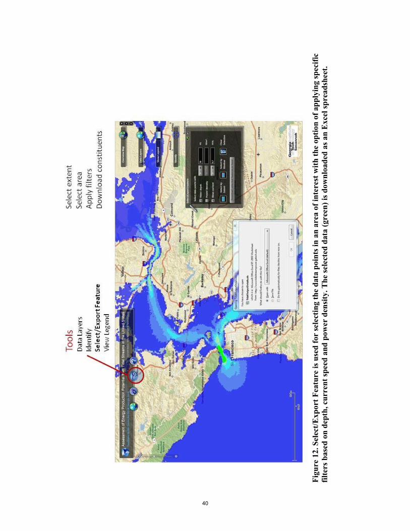
351 Web Server Deployment Originally it was planned to use ArcIMS to develop an interactive web-based GIS system to facilitate the dissemination of the tidal data and deliver the information of energy production potential from tidal streams to interested users This project has three main functions One is to build a map GUI in ArcIMS to allow users to identify the location on the map to extract the tidal constituents of a given location or the nearest survey point The second is to derive the information about the tidal current magnitude and power density as the histogram and time series graphics generated by MATLAB server MATLAB functions are invoked in ArcIMS by passing the tidal constituents to MATLAB server via a REST Web service call To enable the dissemination of the tidal data the third function allows users to extract the tidal data of a given spatial extent The users can either use the map extent of ArcIMS or draw a box to define a specific spatial extent Data extraction can be refined by a combination of three constituents including water depth power density and mean current
Since ArcIMS is the old technology for Web mapping applications ESRI will no longer support ArcIMS in releases after ArcGIS 100 With the adoption of ArcGIS Server and the move to 64-bit servers ArcIMS is no longer the recommended product for producing web maps ArcGIS server offers three APIs (javascript API Flex API and Silverlight API) for Web mapping development In contrast to frame-based ArcIMS the new APIs support the so-called rich internet applications (RIAs) development
Both Javascript API and Flex API were fully developed but eventually Flex API is recommended for this project for several reasons By using the Flash plug-in its cross-platform cross-browser feature help to simplify the GUI design and implementation Particularly the Flex viewer offers much user-friendly and interactive GUI in mapping and arranging the search query results One disadvantage for Flex development is its ActionScript is not standardized but a proprietary script language and has a limited debugging environment
352 Design and Highlights of Data Dissemination The entire suite of data is stored in a geodatabase and made public via the ArcGIS spatial database engine server All of the edits are transferred and synchronized with the data on the production geodatabase which is accessible by multiple editors and then copied to a publication geodatabase for dissemination (Figure 7) The web page interface is a rich internet application (RIA) that facilitates easy navigation over the map with the option for alternative views (GT 2011)
32
Users
Production Geodatabase
Editors
Publication Geodatabase
ArcGIS Server
Figure 7 A production and publication geodatabase approach is used in management of the distributed data for the tidal stream power assessment
Both the database and the web server are hosted in the same workstation with a Dual-Core AMD Optheron Processor 220 GHz 4 GB RAM that runs on Microsoft Windows Server 2003SE SP2 platform The software requirements include the ArcGIS Server for publishing data Matlab Microsoft Visual Studio 2008 for interactive operations and Microsoft Internet Information Services for hosting the website
Assessment of Energy Production Potential from Tidal Streams in United States web page can be accessed at httpwwwtidalstreampowergatechedu address A screenshot of the web page and its main functions is shown in Figure 8 Users can interact with the map using the pull down menus or widgets on the right of the screen Overview map data layers and the legend widgets are displayed on the right of the screen by default It is possible to switch between the satellite and street views via the Map menu while zooming and panning are facilitated with the Navigation menu The web page consists of multiple layers that can be turned on and off through the data layers widget The data layers and interactive tools that can be used for detailed analysis are explained below
Data Layers The data layers widget is shown together with the overview map and the legends widget in Figure 9 The transparency of each layer can be adjusted with a slider in the data layers widget The color mapped raster layers include the water depth the mean current speed (one month average of depth integrated tidal current speed) and the mean kinetic power density (one month average of kinetic power density based on depth integrated tidal current speed) These layers are generated by interpolating the model results from computational grids onto an ArcGIS raster grid with 0003q resolution and are useful for a quick visual examination On the other hand the data points layer contains more detailed information that corresponds to actual model grid points and can be queried through the interactive tools and therefore is more suited for in-depth analyses
Identify tool This tool is used to identify a single data point either by clicking on the map or by a given longitude and latitude The identify tool returns the model water depth meanmaximum tidal current magnitude meanmaximum available kinetic power density and the exact longitude latitude at the selected point Detailed information
33
about the related computational grid can also be accessed via the grid documentation link provided with this tool (Figure 10) The grid documentation includes a map showing the extent of the computational domain and information on the model settings (boundary conditions advection scheme time step bottom friction etc) The calibration statistics are also given in the grid documentation Histograms for tidal current and tidal power density at a selected point can be plotted for any specific year using the identify tool These histograms facilitate an overview of the nature of the tidal stream resource at a location as they display the total hours of availability for different ranges of specific current magnitude (or tidal power density) in a year Similarly time series for water surface elevation and tidal current speed plots and the associated data can be downloaded with the identify tool An example for the year 2011 from a location at San Francisco Bay CA where the model predicts relatively larger currents is shown in Figure 11 The identify tool shows that the one-month mean tidal current magnitude is predicted to be 066 ms at this location while the time series show the range of variation in a year with a mean and maximum of 086 and 203 ms The histogram indicates that more than 5450 hours (~227 days) a year the current speed is larger than 05 ms whereas only 3113 hours (~129 days) a year larger than 08 ms
SelectExport data tool The selectexport data tool is used to download data at selected grid points A single point or multiple points can be selected using the select data tool via the selecting by dragging a window or selecting by the current view extent The selected data can be filtered based on the water depth mean current magnitude or mean power density or a combination of them prior to downloading (Figure 12) This provides users the option to exclude the areas that do not meet certain criteria such as a minimum depth or a minimum speed The selected data is exported to a spreadsheet and for each point it includes 67 columns that display the entire information at regarding geographical coordinates the modeled depth computed water level constituents and tidal current constituents and one-month mean maximum for tidal current speed and tidal stream power density (constituent name amplitude and phase for water level a major and a minor axis amplitude phase and inclination angle for the tidal current)
Once the results are displayed in the identify or selectexport widget the user can switch between the results and selection display using the buttons at the top of each widget Instructions on how to use the web page can be accessed through the Help menu Detailed project information model documentation and contact information are also found under this menu (Figure 13) The project information contains the background information objectives and methodology The computational model generation of the grids and tidal forcing calibration and constituent extraction are explained under the model documentation
For further investigations of tidal stream power resources additional geographical information can be integrated to the analysis The choice of location for a tidal stream power converter farm depends on assessment of a number of criteria including the available power site characteristics and environmental economic and social impacts of the planned project These include available power and the site characteristics such as bathymetry water depth and the geology of the seabed changes in the flow patterns water quality sediment transport climates and related ecological impacts on the aquatic
34
and terrestrial life economic and social impacts based on the increased energy supply for the region and alterations to the marine and land use Although it is not possible to quantify all of these criteria and there are no set rules on how to determine acceptable limits for many of them certain functionalities of GIS can be used to build a decision support system to select suitable locations for tidal stream power conversion (Defne et al 2011a) A list of most suitable areas can be determined based on the level of power density ease of accessibility and the number of environmental conflicts
35
36
FFigu
re 8
Use
rss c
an in
tera
ct ww
ith th
e m
ap u
ssing
the
pull
doow
n m
enus
or
wwid
gets
on
the
rrigh
t of t
he sc
rreen
37
FFigu
re 9
Ove
rvvie
w m
ap d
ataa
laye
rs a
nd th
ee le
gend
wid
getts
are
disp
laye
dd on
the
righ
t oof t
he sc
reen
AAny
of t
he d
ata
poin
ts
wwat
er d
epth
mmea
n cu
rren
t sppe
ed m
ean
kinee
tic p
ower
den
ssity
laye
rs c
an b
e di
spla
yed
on th
e sc
reen
wiith
a p
refe
rred
ttr
ansp
aren
cy
38
FFigu
re 1
0 Id
enntif
y to
ol is
use
dd fo
r da
ta in
quuir
y at
a si
ngle
ppoi
nt (s
how
n ww
ith th
e re
d ar
rrow
her
e) H
istto
gram
s and
timm
e se
ries
cca
n be
plo
tted
ffor
a se
lect
ed yy
ear
and
the
mood
el d
ocum
entaa
tion
for
the
reela
ted
grid
can
be
acce
ssed
39
Figu
re 1
1 T
ime
seri
es fo
r tid
al e
leva
tion
and
curr
ent (
left
) a
nd h
istog
ram
s for
tida
l cur
rent
and
pow
er d
ensi
ty (r
ight
) for
the
poin
t sel
ecte
d in
the
iden
tify
tool
exa
mpl
e in
Fig
ure
10
40
FFigu
re 1
2 S
elec
tExp
ort F
eatu
re is
use
d fo
r se
lect
ing
the
ddata
poi
nts i
n ann
are
a of
inte
reest
with
the
opttio
n of
app
lyin
gg sp
ecifi
c ffil
ters
bas
ed o
nn de
pth
cur
rennt
spee
d an
d poo
wer
den
sity
The
sele
cted
datt
a (g
reen
) is d
owwnl
oade
d as
ann
Exc
el sp
read
sshee
t
41
FFigu
re 1
3 In
strru
ctio
ns o
n ho
ww to
use
the
weeb
pag
e p
roje
ct in
form
atio
n m
odel
doc
umeen
tatio
n an
d co
ntac
t inf
orm
attio
n ca
n be
aac
cess
ed th
rougg
h th
e H
elp
meen
u
4 Products
Publications Defne Z Haas K A Fritz H M (2011) GIS based multi-criteria assessment of tidal stream power potential A case study for Georgia USA Renewable and Sustainable Energy Reviews Volume 15 Issue 5 June 2011 Pages 2310-2321
Defne Z Haas K A Fritz H M (2011) Numerical modeling of tidal currents and the effects of power extraction on estuarine hydrodynamics along the Georgia Coast USA Renewable Energy in press
Defne Z Haas K and Fritz H (2011) Multi-criteria assessment of tidal stream power potential using ArcGIS Submitted to ArcNews March 2011
Defne Z Haas K and Fritz H (2008) Assessment of Tidal Currents along the Atlantic Coast of the Southeast USA for Energy Conversion Case Study for Georgia 2nd International Conference on Ocean Energy Brest France
Presentations Haas K Defne Z Fritz H Jiang L French S Shi X Neary V Stewart K and Smith B (2011) A Database of the US Tidal Stream Power Potential Invited presentation at the 4th Annual Global Marine Renewable Energy Conference Washington DC
Haas K Defne Z Jiang L and Fritz H (2010) Assessment of Tidal Stream Energy Potential for the United States AGU Fall Meeting San Francisco California
Jiang L Haas K Fritz H Defne Z French S Shi X and Smith B (2010) Numerical Modeling of Tidal Streams for Energy Assessment Along the US Coast Presented at the 2010 Ocean Sciences Meeting Portland OR
Haas K Fritz H Defne Z Jiang L French S Shi X and Smith B (2009) Assessment of Power Production Potential from Tidal Streams in the United States Invited presentation at the 2nd Annual Global Marine Renewable Energy Conference Washington DC
Haas K (2010) Invited speaker for Standards and Resource Assessment panel in the OceanTidalStream Power track at the 2010 Hydro Vision International Conference Aug 2010
Haas K (2010) Invited speaker Texas AampM coastal engineering seminar series ldquoAssessment of Tidal Stream Energy Production for the United Statesrdquo Sept 2010
WebsiteDatabases The data is stored in a GIS database accessible via the website httpwwwtidalstreampowergatechedu
42
CollaborationsNetworks Kevin Haas is an expert member of the US Technical Advisory Group for IEC TC-114 working on the specification WG-1ldquoTidal Energy Resource Characterization and Assessmentrdquo
Kevin Haas was an invited participant in the Symposium on Renewable Ocean Energy for North Carolina March 2011
Student Education PhD Student Zafer Defne Advisers Kevin Haas and Hermann Fritz Graduation Spring 2010 Topic Assessment of Wave and Tidal Power Potential Along the Atlantic Coast of the Southeast USA for Energy Conversion
Post Doctoral Fellow Lide Jiang PhD Advisers Kevin Haas and Hermann Fritz February 2009 - June 2010 Topic Assessment of Tidal Stream Power Potential for the United States
Post Doctoral Fellow Zafer Defne PhD Advisers Kevin Haas and Hermann Fritz February 2010 - June 2011 Topic Assessment of Ocean Energy for the United States
43
5 References
ADCIRC (2011) ADCIRC Coastal Circulation and Storm Surge Model lthttpwwwunceduimsccatstidestideshtmgt (Accessed 2011)
Bedard R Previsic M Siddiqui O Hagerman G and Robinson M (2006) North American Tidal In Stream Energy Conversion Feasibility Demostration Project EPRI TP-04-NA Electric Power Research Institute
Carter GS and Merrifield MA (2007) Open boundary conditions for regional tidal simulations Ocean Modelling 18(3-4) 194-209
Chapman DC (1985) Numerical Treatment of Cross-Shelf Open Boundaries in a Barotropic Coastal Ocean Model Journal of Physical Oceanography 15(8) 1060-1075
Defne Z Haas KA and Fritz HM (2011a) GIS based multi-criteria assessment of tidal stream power potential A case study for Georgia USA Renewable and Sustainable Energy Reviews 15(5) 2310-2321
Defne Z Haas KA and Fritz HM (2011b) Numerical Modeling of Tidal Currents and the Effects of Power Extraction on Estuarine Hydrodynamics along the Georgia Coast USA Renewable Energy in press doi101016jrenene201105027
Denham CR (2008) SeaGrid Orthogonal Grid Maker for Matlab US Geological Survey lthttpwoodsholeerusgsgovstaffpagescdenhampublic_htmlseagridseagridhtmlgt (Accessed 2008)
Epler J (2010) Tidal Resource Characterization from Acoustic Doppler Current Profilers University of Washington Seattle
EPRI 2006a Methodology for Estimating Tidal Current Energy Resources and Power Production by Tidal In-Stream Energy (TISEC) Devices EPRI-TP-001-NA-Rev-3
EPRI 2006b Tidal In-Stream Energy Resource Assessment for Southeast Alaska EPRI-TP-003-AK
EPRI 2006c Maine Tidal In-Stream Energy Conversion (TISEC) Survey and Characterization of Potential Project Sites EPRI-TP-003-ME
EPRI 2006d Massachusetts Tidal In-Stream Energy Conversion (TISEC) Survey and Characterization of Potential Project Sites EPRI-TP-003-MA
44
EPRI 2006e New Brunswick Tidal In-Stream Energy Conversion (TISEC) Survey and Characterization of Potential Project Sites EPRI-TP-003-NB
EPRI 2006f Nova Scotia Tidal In-Stream Energy Conversion (TISEC) Survey and Characterization of Potential Project Sites EPRI-TP-003-NS
EPRI 2006g North America Tidal In-Stream Energy Conversion Feasibility Study EPRI-TP-008-NA
ESR (2011) TPXO Earth amp Space Research lthttpwwwesrorgpolar_tide_modelsModel_TPXO71htmlgt (Accessed 2011)
Fraenkel P (2007) Marine current turbines pioneering the development of marine kinetic energy converters Proceedings of the Institution of Mechanical Engineers Part A Journal of Power and Energy 221(2) 159-169
Froberg E (2006) Current Power Resource Assessment Uppsala University Uppsala
Garrett C and Cummins P (2005) The power potential of tidal currents in channels Proceedings of the Royal Society a-Mathematical Physical and Engineering Sciences 461(2060) 2563-2572
GT (2011) Assessment of Energy Production Potential from Tidal Streams in the United Sates Georgia Institute of Technology lthttpwwwtidalstreampowergatechedugt (Accessed 2011)
Haidvogel DB Arango H Budgell WP Cornuelle BD Curchitser E Di Lorenzo E Fennel K Geyer WR Hermann AJ Lanerolle L Levin J McWilliams JC Miller AJ Moore AM Powell TM Shchepetkin AF Sherwood CR Signell RP Warner JC and Wilkin J (2008) Ocean forecasting in terrain-following coordinates Formulation and skill assessment of the Regional Ocean Modeling System Journal of Computational Physics 227(7) 3595-3624
Lee MQ Lu CN and Huang HS (2009) Reliability and cost analyses of electricity collection systems of a marine current farm--A Taiwanese case study Renewable and Sustainable Energy Reviews 13(8) 2012-2021
Lim YS and Koh SL (2010) Analytical assessments on the potential of harnessing tidal currents for electricity generation in Malaysia Renewable Energy 35(5) 1024-1032
Myers L and Bahaj AS (2005) Simulated electrical power potential harnessed by marine current turbine arrays in the Alderney Race Renewable Energy 30(11) 1713-1731
45
NGDC (2008a) Coast Line Extractor National Oceanic and Atmospheric Administration lthttprimmerngdcnoaagovcoastgt (Accessed 2008)
NGDC (2008b) Geodas Grid Translator National Geophysical Data Center lthttpwwwngdcnoaagovmgggdasgd_designagridhtmlgt (Accessed 2008)
NOAA (2008a) Electronic Navigational Charts (ENC) Office of Coast Survey National Oceanic and Atmospheric Administration lthttpnauticalchartsnoaagovmcdencdownloadhtmgt (Accessed 2008)
NOAA (2008b) Tides and Currents National Oceanic and Atmospheric Administration lthttptidesandcurrentsnoaagovindexshtmlgt (Accessed 2008)
NOS (2008a) US Bathymetric amp Fishing Maps Office of Coast Survey National Ocean Service NOAA lthttpmapngdcnoaagovwebsitemggfishmapgt (Accessed 2008)
NOS (2008b) VDatum Vertical Datum Translator NOAAs National Geodetic Survey (NGS) Office of Coast Survey (OCS) and Center for Operational Oceanographic Products and Services (CO-OPS) lthttpvdatumnoaagovgt (Accessed 2008)
Stewart K and Neary V (2011) Validation of the Georgia Tech Regional Tidal CurrentResource Assessment Model and GIS-web Tool Oak Ridge National Laboratory
Sutherland DA MacCready P Banas NS and Smedstad LF (In Press) A Model Study of the Salish Sea Estuarine Circulation Journal of Physical Oceanography in press doi1011752011JPO45401(0)
USFWS (2008) National Wetlands Inventory US Fish amp Wildlife Service lthttpwwwfwsgovwetlandsgt (Accessed 2008)
USGS (2008a) Seamless Server U S Geological Survey lthttpseamlessusgsgovgt (Accessed 2008)
USGS (2008b) Water Data for the Nation National Water Information System US Geological Survey lthttpwaterdatausgsgovusanwisswgt (Accessed 2008)
WikiROMS (2011) Horizontal Boundary Conditions WikiROMS lthttpswwwmyromsorgwikiindexphpBoundary_ConditionsHorizontal_Boundary_ Conditionsgt (Accessed 2011)
Zevenbergen LW Lagasse PF and Edge BL (2004) Tidal Hydrology Hydraulics and Scour at Bridges FHWA NHI-05-077 Ayres Associates
46
APPENDIX A
TOTAL THEORETICAL AVAILABLE POWER FROM TIDAL STREAMS
This appendix includes the maps of locations with considerable tidal stream power based on the simplified analytical calculations of the maximum average power from a tidal stream along a channel following the Garret and Cummins (2005) formulation
47
48
Figu
re A
1 T
otal
theo
retic
al a
vaila
ble
pow
er (M
W) f
rom
tida
l str
eam
s alo
ng th
e M
aine
coa
st (N
orth
)
49
Figu
re A
2 T
otal
theo
retic
al a
vaila
ble
pow
er (M
W) f
rom
tida
l str
eam
s alo
ng th
e M
aine
coa
st (S
outh
)
50
Figu
re A
3 T
otal
theo
retic
al a
vaila
ble
pow
er (M
W) f
rom
tida
l str
eam
s alo
ng th
e M
assa
chus
etts
and
Rho
de Is
land
coa
sts
51
Figu
re A
4 T
otal
theo
retic
al a
vaila
ble
pow
er (M
W) f
rom
tida
l str
eam
s alo
ng th
e N
ew Y
ork
coas
t
52
Figu
re A
5 T
otal
theo
retic
al a
vaila
ble
pow
er (M
W) f
rom
tida
l str
eam
s alo
ng th
e N
ew J
erse
y co
ast
53
Figu
re A
6 T
otal
theo
retic
al a
vaila
ble
pow
er (M
W) f
rom
tida
l str
eam
s alo
ng th
e D
elaw
are
Mar
ylan
d V
irgi
nia
coas
ts
54
Figu
re A
7 T
otal
theo
retic
al a
vaila
ble
pow
er (M
W) f
rom
tida
l str
eam
s alo
ng th
e N
orth
Car
olin
a co
ast (
Nor
th)
55
Figu
re A
8 T
otal
theo
retic
al a
vaila
ble
pow
er (M
W) f
rom
tida
l str
eam
s alo
ng th
e N
orth
Car
olin
a co
ast (
Sout
h)
56
Figu
re A
9 T
otal
theo
retic
al a
vaila
ble
pow
er (M
W) f
rom
tida
l str
eam
s alo
ng th
e So
uth
Car
olin
a co
ast
57
Figu
re A
10 T
otal
theo
retic
al a
vaila
ble
pow
er (M
W) f
rom
tida
l str
eam
s alo
ng th
e G
eorg
ia c
oast
Figure A11 Total theoretical available power (MW) from tidal streams along the Florida coast (North East)
58
59
Figu
re A
12 T
otal
theo
retic
al a
vaila
ble
pow
er (M
W) f
rom
tida
l str
eam
s alo
ng th
e Fl
orid
a co
ast (
Sout
h an
d th
e K
eys)
Figure A13 Total theoretical available power (MW) from tidal streams along the
Florida coast (South East)
60
61
Figu
re A
14 T
otal
theo
retic
al a
vaila
ble
pow
er (M
W) f
rom
tida
l str
eam
s alo
ng th
e Fl
orid
a co
ast (
Nor
th E
ast)
62
Figu
re A
15 T
otal
theo
retic
al a
vaila
ble
pow
er (M
W) f
rom
tida
l str
eam
s alo
ng th
e A
laba
ma
Lou
isia
na a
nd T
exas
coa
st
Figure A16 Total theoretical available power (MW) from tidal streams along the California coast (South)
63
Figure A17 Total theoretical available power (MW) from tidal streams along the California (North) and Oregon coast
64
Figure A18 Total theoretical available power (MW) from tidal streams along the Washington coast
65
66
Figu
re A
19 T
otal
theo
retic
al a
vaila
ble
pow
er (M
W) f
rom
tida
l str
eam
s alo
ng th
e A
lask
a co
ast
(Sou
th E
ast 1
)
67
Figu
re A
20 T
otal
theo
retic
al a
vaila
ble
pow
er (M
W) f
rom
tida
l str
eam
s alo
ng th
e A
lask
a co
ast
(Sou
th E
ast 2
)
68
Figu
re A
21 T
otal
theo
retic
al a
vaila
ble
pow
er (M
W) f
rom
tida
l str
eam
s alo
ng th
e A
lask
a co
ast
(Sou
th 1
)
69
Figu
re A
22 T
otal
theo
retic
al a
vaila
ble
pow
er (M
W) f
rom
tida
l str
eam
s alo
ng th
e A
lask
a co
ast
(Sou
th 2
)
70
Figu
re A
23 T
otal
theo
retic
al a
vaila
ble
pow
er (M
W) f
rom
tida
l str
eam
s alo
ng th
e A
lask
a co
ast
(Sou
th W
est)
71
Figu
re A
24 T
otal
theo
retic
al a
vaila
ble
pow
er (M
W) f
rom
tida
l str
eam
s at A
leut
ian
Isla
nds
AK
(Ea
st 1
)
72
Figu
re A
25 T
otal
theo
retic
al a
vaila
ble
pow
er (M
W) f
rom
tida
l str
eam
s at A
leut
ian
Isla
nds
AK
(Ea
st 2
)
73
Figu
re A
26 T
otal
theo
retic
al a
vaila
ble
pow
er (M
W) f
rom
tida
l str
eam
s at A
leut
ian
Isla
nds
AK
(W
est 1
)
74
Figu
re A
27 T
otal
theo
retic
al a
vaila
ble
pow
er (M
W) f
rom
tida
l str
eam
s at A
leut
ian
Isla
nds
AK
(W
est 2
)
75
Figu
re A
28 T
otal
theo
retic
al a
vaila
ble
pow
er (M
W) f
rom
tida
l str
eam
s at A
leut
ian
Isla
nds
AK
(W
est 3
)
76
Figu
re A
29 T
otal
theo
retic
al a
vaila
ble
pow
er (M
W) f
rom
tida
l str
eam
s at A
leut
ian
Isla
nds
AK
(W
est 4
)
APPENDIX B
REPRINTS OF PUBLISHED PAPERS
This appendix includes reprints of the published journal and conference papers
Defne Z Haas K A Fritz H M (2011) GIS based multi-criteria assessment of tidal stream power potential A case study for Georgia USA Renewable and Sustainable Energy Reviews Volume 15 Issue 5 June 2011 Pages 2310-2321
Defne Z Haas K A Fritz H M (2011) Numerical modeling of tidal currents and the effects of power extraction on estuarine hydrodynamics along the Georgia Coast USA Renewable Energy in press
Defne Z Haas K and Fritz H (2008) Assessment of Tidal Currents along the Atlantic Coast of the Southeast USA for Energy Conversion Case Study for Georgia 2nd International Conference on Ocean Energy Brest France
77
Renewable and Sustainable Energy Reviews 15 (2011) 2310ndash2321
Contents lists available at ScienceDirect
Renewable and Sustainable Energy Reviews
journa l homepage wwwelsev ier com locate rser
GIS based multi-criteria assessment of tidal stream power potential A case study for Georgia USA
Zafer Defne lowast Kevin A Haas Hermann M Fritz Georgia Institute of Technology 210 Technology Circle Savannah GA 31407 United States
a r t i c l e i n f o a b s t r a c t
Article history Received 19 October 2010 Accepted 28 January 2011
Keywords Site selection In-stream converters North Atlantic
A multi-criteria assessment methodology that accounts for the physical environmental and socioeco-nomic constraints is proposed to assist in the selection of the most suitable locations for tidal stream power conversion projects For this purpose the tidal stream power resource data are incorporated into a Geographical Information System (GIS) database together with datasets that are related to different aspects of the site selection methodology The proposed method is applied to the Georgia coast to find and rank the best locations for power conversion The suitable areas are narrowed down to a subset of the high power density areas that satisfy the constraints of a tidal stream power conversion scheme A demonstrative ranking procedure with equal weighting factors for all criteria shows that the Savan-nah Ogeeche Canoochee and Medway Rivers and the Cumberland Sound have the best locations for tidal power conversion on the coast of Georgia This methodology is also applicable to other sites where sufficient geospatial data are available
copy 2011 Elsevier Ltd All rights reserved
Contents
1 Introduction 2310 2 Literature review 2311
21 Factors related to tidal stream power conversion 2311 22 Use of GIS in site selection 2313
3 Methodology 2313 31 Data coverage and classification 2314
311 Physical realization layer 2314 312 Environmental constraints layer 2315 313 Socioeconomic constraints layer 2315
32 Identification of map regions 2315 33 Ranking of suitable locations 2317
4 Site selection methodology applied to Georgia coast 2319 5 Conclusions 2320
Acknowledgements 2320 References 2320
1 Introduction
Given the current and projected global energy demand and the associated impact on the environment marine energy conversion projects offer viable alternatives with their clean and renewable applications There are many projects and emerging technologies worldwide to convert the power from the vastly unexploited ocean
lowast Corresponding author Tel +1 912 965 2393 E-mail addresses zaferdefnegatechedu (Z Defne) khaasgatechedu
(KA Haas) fritzgatechedu (HM Fritz)
1364-0321$ ndash see front matter copy 2011 Elsevier Ltd All rights reserved doi101016jrser201102005
tides and currents to electric power Resource mapping is a funda-mental step in development of such projects given the distributed nature of these resources In order to provide this step for any pos-sible future developments in the state of Georgia the wave power potential and the tidal stream power resource in the region have been investigated [12] The wave power was found to diminish sig-nificantly on the broad continental shelf with the regions of larger power being limited to the offshore portion of the shelf The tidal stream power on the other hand was determined to be substan-tially amplified at some of the locations along the shoreline at some specific parts of the Savannah Canoochee Ogeeche Altamaha and Medway Rivers and the Intercoastal Waterway between the
2311 Z Defne et al Renewable and Sustainable Energy Reviews 15 (2011) 2310ndash2321
Fig 1 Mean power density maps along (a) the northern and (b) the southern coasts of Georgia
Altamaha and the Doboy Sounds as well as St Catherines Sapelo St Andrews and Cumberland Sounds (Fig 1) Here a comprehen-sive methodology to analyze the tidal stream power potential in the context of the physical environmental and social constraints using GIS tools has been developed
This paper is organized as follows First the factors related to the tidal stream conversion projects are discussed along with the liter-ature on use of GIS as a decision support tool for energy projects Then the data coverage and the methodologies for identification and ranking of the suitable locations are presented in detail fol-lowed by the application to the Georgia coast to determine the most promising locations for tidal stream power conversion Finally the concluding remarks and suggestions for future work are presented
2 Literature review
Recently the International Electrotechnical Commission (IEC) has initiated international standards for marine power conversion systems TC 114 Marine Energy-Wave and Tidal Energy Converters which addresses the evaluation and mitigation of environmental impacts resource assignment requirements performance mea-surement of converters and other related issues [3] Since there is no international standard available at the present the current study relies upon the methodologies and experiences from other marine renewables and wind power conversion projects
21 Factors related to tidal stream power conversion
The choice of location for a tidal stream power converter farm depends on assessment of a number of criteria including the avail-
able power site characteristics and environmental economic and social impacts of the planned project [4ndash10] The available power and the site characteristics such as bathymetry water depth and the geology of the seabed constitute the physical constraints of analysis which are easier to assess quantitatively than the envi-ronmental economic and social constraints with modeling and measurements
The environmental impacts can be grouped as the physical impacts such as changes in the flow patterns and water quality and related ecological impacts on the aquatic and terrestrial life The effect on water quality during installation mainly consists of disturbance to the sediment which results in suspension of sedi-ment and increased turbidity This is of more concern if the bottom sediment has contamination During operation converters alter the tidal energy flow hence the sedimentation patterns and suspension as well as the vertical mixing Scour and loss of soft sediments might occur near the structures
In order to avoid the adverse impact on aquatic life habitats for endangered protected or sensitive species should be clearly identified and avoided if possible Because suspension of fine sed-iment due to construction may have impacts on the immediate surroundings fish spawning or nursery areas and sensitive benthic habitat should be avoided While the effect of noise and vibra-tion on aquatic life during operation is a research topic for the ongoing projects noise and vibration during construction might be more critical especially during breeding nesting and migration seasons However these can be minimized by careful site selec-tion and timing for the project [7] The mechanical and flow related injuries of the aquatic life from conventional hydropower facilities include impingement with screens and contact with the blades
2312 Z Defne et al Renewable and Sustainable Energy Reviews 15 (2011) 2310ndash2321
Environmental Constraints Layer
Socioeconomic Constraints Layer
Physical Realization Layer
NGDC (NOAA)
User InputUSGS
ESI (NOAA) USFWS
ENC (NOAA)CENSUS
Candidate Locations for Tidal Power Conversion
DNR
Site Selection and Ranking Methodology
Fig 2 Structure of geographically referenced information and the underlying data sources used for selecting candidate locations for tidal power conversion
and abnormal changes in pressure gradients and water velocities Although converters with unenclosed turbines look similar to boat propellers or hydroelectric power turbines they operate at much lower speeds and much lower pressures than those traditional devices The blades are usually slender and the percentage of area swept by the rotor is much smaller This reduces the probability of fish passing through making contact with the blades Injury from impingement abrasion pinching or grinding is prevented in the absence of a screen of a shroud The installation stage may also require permanent removal of some terrestrial habitat to construct the shore station access roads and right of way for the transmission lines [7] The disturbance to the wetlands should be kept at mini-mum and temporary as much as possible and permanent changes to the hydrology of the wetlands should be investigated [11]
The economic and social impacts can be evaluated based on the increased energy supply for the region and alterations to the
Table 1
marine and land use Commercial activities such as shipping and fishing usually share the sea space with recreational and touristic activities However during the installation of converters most of land and marine activities in the vicinity of the project area need to be restricted At the operation stage fishing exclusion zones and restricted areas for recreational boats may need to be introduced If navigation or commercial shipping cannot be avoided enough safety clearance should be left between the rotor blade and the devices at lowest astronomic tides The aesthetical concerns and the effects on the cultural and historic sites are additional aspects to be considered when evaluating the environmental effects [5]
Some positive environmental impact may be expected from the converters Establishing fishing exclusion zones around convert-ers may help increasing the amount of aquatic life by providing shelter for marine life Project structures such as transmis-sion cables may serve as suitable structures for invertebrates
List of layers sources and themes and their roles NA indicates the themes that are not assigned any roles
Layer Source Theme Role
Physical realization NGDC Coastline Outlines and Filters ESI Bathymetry NOAA Hydrology layer User data Tidal power map
Environmental constraints ESI Fish (E) Critical Areas NOAA Invertebrates (E) USGS Reptiles (E) USFWS Birds (E) DNR Mammals (E)
Plants and habitats (E) Socioeconomic constraints CENSUS Urbanized areas Favorable Areas
USGS Transmission DOE Transportation DOT Built-up areas ENC Restricted areas Restricted Areas NOAA Fairways and shipping lines
Dumping sites Cable areas Pipeline areas Shoreline constructions Wreck points Mooring and warping points Recreation areas and access locations (Boat ramps diving sites marinas) Management areas (Marine sanctuary national parks wildlife refuges special management areas) Cultural heritage sites (Archeological sites historical sites) Resource extraction sites NA (Aquaculture sites commercial fisheries recreational fishing)
2313 Z Defne et al Renewable and Sustainable Energy Reviews 15 (2011) 2310ndash2321
Fig 3 Demonstration of information from physical socioeconomic and environmental constraints layers presented on the same map for Savannah River Wassaw and Ossabaw Sounds
and macro algae developing an artificial reef for the aquatic community [5]
22 Use of GIS in site selection
Although it is not possible to quantify all of these criteria their evaluation to minimize the consumption of material and energy requires integration of a significant amount of information which makes utilizing GIS tools extremely beneficial [12] For the last 20 years GIS applications have been successfully used to assess environmental and economic constraints and to select suitable sites for energy projects [13ndash30] The suitability of GIS to serve for this purpose was proposed earlier [12] while its performance and shortcomings having been evaluated more recently [31] A deci-sion support system to site wind power conversion projects was first defined in 1980 [23] The system involved resource analysis quantifying the proximities to areas of interest or special impor-tance and excluding the restricted areas The results were ranked and synthesized in a matrix in order to identify the most suitable locations Through the years there has not been significant change in the methodology and in 2000 a GIS-based approach with a sim-ilar methodology was used to evaluate sites for wind farms in the
UK [15] Although there are significant differences between them [93233] the essentials of wind power and tidal stream power con-version are close enough that a similar workflow can be created to assess the suitability of locations for tidal stream power conver-sion projects Recently more comprehensive approaches became available such as the marine resource assessment of the UK [34] and the Ocean Special Area Management Plan in the state of Rhode Island [35] which can provide guidelines for future studies There are no set rules on how to determine acceptable limits for changes to the currents and sediment transport climates caused by current energy extraction devices Reports on assessing the tidal power potential of North America focusing on a few specific regions with high potential to identify the environmental impacts and economic constraints and assess the available technologies for suitability and other related studies can be used as a guide for determining the related factors [83637]
3 Methodology
This section describes how the various data and constraints are incorporated into a decision making tool to assist in the site selec-tion First the data from various sources are compiled in a GIS
2314 Z Defne et al Renewable and Sustainable Energy Reviews 15 (2011) 2310ndash2321
Transmission amp Transportation
Masked Critical
Critical Themes Favorable Themes Restricted Themes
Filter Bathymetry
Merge Merge
Favorable Subset Restricted
Calculate Distance from Suitable Locations
Environmental Score Map
Suitable Locations
Distance to Favorable
Distance to Transportation
Suitability Score Map
Distance to Transmission
Filter Power Density
Exclude Restricted
Filtered Superset 2 Filtered Superset 1
Intersect
Filtered Subset
Mask Power Density
Mask Critical Themes
Power Density Score Map
Bathymetry Power Density
Normalize amp Weighted Overlay
Filtered Power Density
Normalize amp Overlay
Normalize
Accessibility Score Map
Normalize amp Weighted Overlay
Fig 4 Flow diagram of the site selection methodology for tidal power conversion Ovals represent actions and rectangles represent objects
environment and the themes in each dataset are classified into conceptual layers Then map regions are identified according to the role of each theme in tidal stream power conversion Finally the suitable locations are determined and the ranking algorithm is applied to calculate the score for each location and determine the best areas for tidal stream power project siting The data coverage definition of conceptual layers and the details of the identification and ranking algorithms are discussed in details within this section
31 Data coverage and classification
A large amount of GIS data is available online scattered between governmental offices science centers and the private sector which requires significant amount of work to compile The GIS portals such as the Georgia GIS Data Clearing House [38] and the Geo-data [39] facilitate the retrieval of state wide and country wide geographic data respectively However the data origins still vary resulting in different datums projections scales and resolutions Some of the data may be formatted to be used with specific software packages and on specific platforms Hence the attached metadata needs to be examined for compatibility and conversion between the datasets After an extensive investigation of online resources the number of related sources is reduced down to a set of major data
providers according to their coverage of information data quality and accessibility These major sources include National Oceanic and Atmospheric Administration (NOAA) through Electronic Naviga-tional Charts (ENC) National Geophysical Data Center (NGDC) and Environmental Sensitivity Index Maps (ESI) and United States Geo-logical Survey (USGS) United States Census Bureau (CENSUS) and Environmental Protection Agency (EPA) State and local environ-mental information can also be accessed at Georgia Department of Natural Resources (DNR) and US Fish amp Wildlife Service (USFWS)
The geospatial data gathered from various sources are catego-rized into three conceptual layers The physical realization layer the environmental constraints layer and the socioeconomic con-straints layer (Fig 2) These layers include the information on the basic geometry and physics of the problem areas that are of envi-ronmental concern and areas of social and economic concern respectively
311 Physical realization layer The physical layer consists of the 170000 scale medium reso-
lution shoreline from NOAA the digital sounding data from NGDC as the bathymetry and the tidal stream power density map This layer defining the physical boundaries and the amount of kinetic power per unit cross-sectional area contains the most essential
2315 Z Defne et al Renewable and Sustainable Energy Reviews 15 (2011) 2310ndash2321
Fig 5 (a) All exclusive (red) critical (yellow) and favorable (green) areas for tidal stream power conversion in Savannah River Wassaw and Ossabaw Sounds Bathymetry filtered by a minimum depth of 5 m (b) Tidal power density filtered by a minimum of 250 Wm2 (For interpretation of the references to color in this figure legend the reader is referred to the web version of the article)
data for the site selection scheme One of the important factors is the depth of flow which is used to verify the necessary verti-cal space to allocate the tidal power converters Despite including the essential data the physical layer itself alone is not sufficient to perform a rigorous multi-criteria assessment
312 Environmental constraints layer All plants animals and microorganisms and the non-living phys-
ical factors of an environment is called the ecosystem of that area Tidal stream power converters with their slow motion which may be avoided easily by fish and other sea animals [5] and low noise levels are expected to have low impact on the ecosystem of an area Nevertheless it is still necessary to evaluate their possible interference with the ecosystem further especially where endan-gered species are present This study does not attempt to answer these questions but only use the related findings available in the literature Environmental considerations require mapping of the endangered species habitats and avoiding these locations wherever possible Although they are mainly prepared for oil and chemical spill response purposes ESI maps provide some essential data such as sensitive biological resources and seabird colonies that can be used in the site selection methodology [40] Detailed information on the threatened and endangered species in Georgia can also be obtained from USFWS Endangered Species and Georgia Ecologi-cal Services [4142] The GIS data from this source is merged with ESI data for the environmental constraints layer Supplementary data are provided from Georgia Environmental Resources Digital Data Atlas which is served by USGS Center for Spatial Analysis Technologies [43]
313 Socioeconomic constraints layer The socioeconomic constraints layer contains the related human
activities in the region ENCs provided to the public by NOAArsquos Office of Coast Survey are vector-based digital files containing marine features suitable for marine navigation and GIS applications and usually used for route planning [44] They carry information on the manmade structures and marine activities The census data pro-vides information about built-up areas classified by their surface area and the size of inhabiting population Some of the supplemen-tal data such as transportation and transmission lines can be found in Georgia Environmental Resources Digital Data Atlas The loca-tion and orientation of transmission lines and the roads are some of the important factors for power conversion projects ESI maps also provide some socioeconomic information which includes but not limited to location of boat ramps historical sites and aqua-
culture and fishing sites Sensitive human-use resources such as water intakes marinas and swimming beaches are also marked in ESI maps
32 Identification of map regions
The suitable areas are determined based on the level of power density ease of accessibility and the number of environmental con-flicts with the site selection methodology For this purpose each theme is tagged according to its role in the tidal stream power con-version The list of themes their roles sources and the layers that they belong to are presented in Table 1 The themes in the phys-ical realization layers are used to set the physical constraints and boundaries of the problem and are tagged ldquooutlines and filtersrdquo The themes with sensitive biological resources data are tagged as ldquocriticalrdquo whereas the themes where it is socioeconomically more advantageous to have the power conversion projects closer are tagged as ldquofavorablerdquo and the themes where the placement of a tidal power converter would not be allowed or should be avoided are tagged as ldquorestrictedrdquo An example of most of the data themes excluding the tidal power density data are shown on a coastline sec-tion that includes a part of Savannah River Wassaw and Ossabaw Sounds in Fig 3 The definition and classification of each theme is discussed in the following paragraphs
The critical areas include the habitats of endangered species which are at risk of becoming extinct Endangered species are usu-ally under legal protection and human activities in the proximity of their habitat are limited Therefore the list of the sensitive biolog-ical resources acquired from the GIS database is filtered to include only the species that are listed as endangered on the state or federal lists of endangered species This is denoted by appending the theme name is appended with ldquo(E)rdquo in Fig 3 and Table 1 The endangered marine mammals along the Georgia coast include whales and man-atees Given their size and offshore habitats the whales are not as common as manatees in shallow estuaries and tidal creeks of the Georgia coast High-use areas for the endangered West Indian Man-atee species are Cumberland St Andrews and St Simons Sounds on the south and Savannah River on the north (Figs 1 and 3) The offi-cial state marine mammal of Georgia the Northern Right Whale is known to prefer areas offshore of Cumberland St Andrews and St Simons Sounds for breeding The second-largest living animal and an endangered species the Fin Whale can be found at offshore of Georgia (Grayrsquos Reef National Marine Sanctuary) at certain times of year Reptiles (E) and Fish (E) in Georgia include the Green Sea Turtle and the Shortnose Sturgeon respectively The Shortnose Sturgeon
2316 Z Defne et al Renewable and Sustainable Energy Reviews 15 (2011) 2310ndash2321
Fig 6 (a) Tidal power density in the Savannah River Wassaw and Ossabaw Sounds filtered by a minimum of 250 Wm2 5 m depth and with restricted areas removed (b) Normalized distance to transportation lines from the suitable locations for tidal stream power conversion
inhabits Savannah Canoochee and Altamaha Rivers whereas the Green Sea Turtle is observed mostly at Grayrsquos Reef The endangered bird species in the coastal Georgia are limited to Wood Stork which have their nests scattered across the coastal zone (Fig 3) Although Bald Eagles are listed as endangered in ESI maps they were reclas-sified from endangered to threatened in 1995 by USFWS and were removed from the USA federal governmentrsquos list of endangered species in 2007 [45] Threatened species such as Frost Flatwoods Salamander and Indigo Snake or the plants classified as Species of Concern (C) such as Pondspice are not considered to be critical since they are not a part of endangered species [41]
Power from converters is anticipated to promote the local activities and developments in the coastal zone therefore socioe-conomic considerations favor the locations that are closer to the socially developed areas such as urbanized and built-up areas where most of the demand is located An urbanized area is defined as a densely settled territory that contains 50000 or more peo-ple [46] The extent of the urbanized areas is based on the CENSUS 2000 data (Fig 3) Built-up locations are defined as a concentra-tion of buildings supporting road or rail infrastructure [47] Airports and US Coast Guard facilities are considered as parts of built-up areas Electric power transmission and all ground transportation are respectively indicated as transmission lines and transportation lines in Fig 3 The right of way for the transmission lines and for the roads to access the selected area is another important decision factor The right of way represents a big part of the cost of construc-tion and it may also disturb the immediate nature and habitat [5] It is desired to keep the right of way for the transmission and the access roads as short as possible Therefore the proximity of the power conversion projects to the main power grid for connection and to the transportation grid for easy access is also advantageous
The restricted areas need to be excluded from tidal power con-version projects due to their potential impact on the environment and on the existing use of sea space The areas managed by the USFWS as National Wildlife Refuges or by Georgia DNR as State Wildlife Management Areas are shown as Wildlife Refuge in Fig 3
National parks include national parks seashores and monuments managed by the National Park Service Marine sanctuaries denote the areas managed by the NOAA Sanctuary and Reserves Division as National Marine Sanctuaries and as National Estuarine Research Services by NOAA and the state These areas and together with areas designated by an appropriate authority within which navi-gation is restricted in accordance with certain specified conditions are marked as possible exclusive areas for tidal stream power con-version projects Fairway is defined as a part of a river where the main navigable channel for vessels of larger size lies ie ship-ping channel a mooringwarping facility is the structure used to secure a vessel and a dumping site is a sea area where dredged material or other potentially more harmful material is deliberately deposited [47] Pipeline areas consist of a string of intercon-nected submarine or overhead pipes used for transport of matter such as oil or gas All fairways dredged areas mooringwarping facilities dumping sites historical sites and pipeline areas are considered as parts of the restricted areas Recreation areas includ-ing boat ramps diving sites and marinas are also considered as restricted
General areas where commercial fishing activities take place are marked with specific symbols in Fig 3 Recreational fishing is abun-dant along the Georgia coast hence omitted Locations for farming of freshwater and saltwater organisms are marked as aquaculture sites on the map Some of these locations of interests such as aqua-culture commercial fishing are not included in the site selection methodology at this stage The benefits and the impact of tidal power conversion on these require special feasibility and design studies and should include discussions and communications with all of the interested parties Similarly piles obstructions beaches access locations and water intakes are not considered as factors for site selection
A flow diagram that shows the steps in the implementation of the site selection methodology is provided in Fig 4 Regardless of their design most of the tidal stream power converters have a min-imum depth requirement based on their dimensions Additionally
Table 2 Ranking results for tidal power conversion along the Georgia coast at selected locations shown in Figs 7 and 8
Point Lon Lat Power density score (P) Environmental score (E) Accessibility score (A) Overall suitability score (S) Rank
A minus81029 32087 05 07 08 053 2 B minus81127 31857 06 03 05 030 5 C minus81265 31755 05 10 06 063 1 D minus81182 31539 02 10 05 036 4 E minus81344 31327 06 00 04 010 6 F minus81448 30708 04 07 08 050 3
2317 Z Defne et al Renewable and Sustainable Energy Reviews 15 (2011) 2310ndash2321
Fig 7 Candidate locations with tidal power conversion potential on the northern Georgia coast that are determined by applying the site selection methodology
there is usually a minimum flow speed (ie cut-in speed) that is required for the devices to start extracting power from the flow The geospatial data for the power density and the bathymetry are filtered by minimum values to get the maps for filtered supersets (Fig 4 top left) The intersection of these two supersets gives the filtered subset The themes with restricted areas are merged into a single theme called restricted after applying certain buffer areas around the features (Fig 4 top middle) and then excluded from filtered subset to determine the suitable locations Similarly the themes that contain the favorable locations are also merged into a single polygon The habitats of endangered species are extracted from the GIS database and specific buffer zones are applied around them based on the federal and state regulations The map of suitable locations is used to mask the power density and the critical areas maps in order to calculate the scores for these locations Likewise the distances to favorable areas and transmission and transporta-tion lines from the suitable locations are computed to facilitate
the calculation of the accessibility scores Finally these scores are normalized and overlaid on the map to determine the candidate locations for tidal power density conversion For normalizing each map the maximum score in that map is used so that the data values range between 0 and 1 1 being the best score
33 Ranking of suitable locations
The site selection methodology can serve as a useful prelimi-nary analysis tool for decision makers before allocating resources for a more detailed evaluation Consequently the criteria for rank-ing the candidate sites can be simplified to three essential scores related to the level of power density accessibility of the site and the environmental challenges
Normalized power density and the normalized environmental constraint are used to define two of the scores whereas the nor-malized distances are combined into a single term to define the
2318 Z Defne et al Renewable and Sustainable Energy Reviews 15 (2011) 2310ndash2321
Fig 8 Candidate locations with tidal power conversion potential on the southern Georgia coast that are determined by applying the site selection methodology
accessibility score It is important to note that the accessibility score is related to economics but it is not used in the ranking algorithm here since an economic analysis is beyond the scope of this study
The power density for every point is normalized with the max-imum power density in the potential areas using
PD P = (1)
PDmax
where P is the power density score PD is the power density at a point and PDmax is the maximum power density within the suitable areas (ie Filtered Power Density in Fig 4) so that the point with the highest power density scores 1
Each distinct conflict with the environmentally sensitive loca-tions on the filtered critical areas map is itemized and the values on the map are normalized with the total number of possible conflicts
using
NE E = 1 minus (2)
NEmax
where E is the environmental score NE is the number of conflicts at a point and NEmax is the maximum number of conflicts For exam-ple if the maximum possible number of conflicts is 4 a point in the buffer zone for the endangered bird species gets 075 whereas another point that lies on the intersection of the buffer zone of the endangered bird species and endangered fish gets 05 The point that has all possible conflicts gets a score of 0
The distances to transportation and transmission lines and to favorable areas from every point on the suitable areas are computed and normalized so that the closest point to the transmission lines gets a score of 1 and the most distant location gets 0 The normalized
2319 Z Defne et al Renewable and Sustainable Energy Reviews 15 (2011) 2310ndash2321
Fig 9 The power density (P) accessibility (A) and environmental (E) scores of tidal power conversion along the Georgia coast at selected locations shown in Figs 7 and 8
values are combined to get the accessibility score by (
km DTM kp DTP A = 1 minus middot + middot
km + kp + kf DTMmax km + kp + kf DTPmax
)kp DTF + middot (3)
km + kp + kf DTFmax
where A is the accessibility score DTM DTP and DTF are distances to transmission and transportation lines and favorable areas respec-tively The terms km kp and kf are weighting coefficients which are assumed to be equal in this study Finally the three scores are used to generate a triangular Kiviat diagram (radar chart) The quality of each location for tidal power conversion is computed from the area under the triangle using the formula
kp middot P middot ka middot A + kp middot P middot ke middot E + ka middot A middot ke middot E S = (4)
kp middot ka + kp middot ke + ka middot ke
where kp ka and ke are the weighting coefficients for P A and E respectively S is the overall suitability score nondimensionalized by the maximum possible area A triangle with a larger area corre-sponds to a higher overall suitability score hence a higher rank In this study power density accessibility and environmental scores are assumed to have equal weights and the nondimensional suit-ability score is calculated by
P middot A + P middot E + A middot E S = (5)
3
4 Site selection methodology applied to Georgia coast
The methodology is applied to the entire Georgia coast how-ever intermediate steps are illustrated on a smaller section of the coastline which consists of the Savannah River Ossabaw and Was-saw Sounds (Figs 5 and 6) All merged favorable restricted and critical areas are shown in green red and yellow respectively in Fig 5a where the circles with various sizes indicate the buffers cre-ated around the locations of interest The size of the buffer is based on the related regulations whenever information is available or a reasonable distance is determined based on the satellite imagery All boat ramps mooringwarping locations marinas and coast-guard are marked with a 400 m buffer The locations indicated as
hazardous in the original are applied 800 m buffer Restricted nav-igation pipelines dumping ground fairway dredged area cable locations and the special management areas are already defined as polygons in the original datasets and no buffer is required for these areas Similarly the urbanized area polygons are used as is whereas all airports and built-up locations have a 100 m buffer The spatial distribution of the endangered species other than the Wood Storks is provided as polygons in the original datasets and is used as is for the site selection methodology Based on the environ-mental regulations the nest locations have a buffer zone of 800 m [4142] Correspondingly the same distance is used for creating buffer zones around boundaries of the special management areas such as wildlife refuges and national parks
There is no standard for the size of power conversion devices and most of the existing devices and prototypes are built to meet the requirements of a certain project with the dimensions of the devices changing from several meters to tens of meters [4849] Since the analysis in this study does not depend on a specific device and given the limited depth in Georgia coastal waters the min-imum depth is chosen to be 5 m large enough to accommodate a small size conversion device with the existing technology The bathymetry filtered by 5 m for the Savannah River Wassaw and Ossabaw Sounds is shown as an example in Fig 5a It is seen in this figure that the 5 m filter already removes a substantial amount of area from the whole domain leaving only limited areas along the main rivers and part of the sound entrances
The cut-in speeds for the tidal power conversion devices range from 05 ms to 1 ms depending on their design Although some studies that simulate power extraction acknowledge cut-in speed values for the horizontal axis turbines as large as 1 ms [5051] there are many examples with cut-in speeds around 07 ms and a vertical axis turbine with 05 ms [495253] The minimum for the power density is selected as 250 Wm2 which corresponds to a flow speed of 08 ms The example of the filtered power density for the pilot area is shown in Fig 5b The larger power density is con-stricted to the rivers and river mouths for this example When the restricted areas are excluded from the subset of locations filtered for depth and the power density the potential areas for tidal power conversion reduce drastically (Fig 6a) The normalized distance to transportation lines from the suitable areas for the pilot region is
2320 Z Defne et al Renewable and Sustainable Energy Reviews 15 (2011) 2310ndash2321
shown in Fig 6b as an example demonstrating that a location with larger power may not have ease of access which is likely to add up to the cost of a project
The suitability score maps for the north and the south sections of the coast are shown in Figs 7 and 8 respectively after all nor-malized maps are overlaid on the entire Georgia coast Based on the power density score map St Catherines Sapelo and Cumberland Sound entrances and the Ogeechee Canoochee and Altamaha River mouths are found to have large areas of candidate sites for power conversion with the Cumberland Sound having the largest power density amongst all The Canooche and Medway rivers have con-siderably higher power density over a substantially large area that meets the criteria and there are few isolated patches of very small areas such as Savannah River and upstream Altamaha River It is seen in Figs 7 and 8 that some of the areas with large power den-sity presented in Fig 1 are eliminated and a more useful subset of suitable areas is obtained when the methodology developed here is applied to the Georgia coast The maximum suitability score is found to be 078 which is less than 1 meaning that none of the suit-able locations is perfect in meeting all of the criteria The locations with the highest suitability scores are discovered in the Savannah Ogeechee Canoochee Medway Rivers and the Cumberland Sound considering equal weights for each criterion
Six locations that have larger power density relative to their surrounding area are selected from the candidate areas to demon-strate the use of site selection methodology as a decision support tool Labeled A to F from North to South respectively these loca-tions are in the Savannah Canoochee and Medway Rivers Sapelo Sound Altamaha River and Cumberland Sound The ranking scores for these locations are shown on Kiviat diagrams in Fig 9 and the results are summarized in Table 2 Based on the ranking algorithm Location E is ranked the worst of the six locations since it has a conflict with all possible critical areas and has low accessibility Location B is also one of the environmentally disadvantageous loca-tions although it has a moderate power density Location D and F are more preferable than locations B and E Location D has no environmental conflict but considerably less power than all other locations while location F is more accessible and has a larger power density but not as environmentally friendly as location D There-fore ranking between these two locations requires a more detailed analysis On the other hand location A has larger power density than location D and ranks better than D and F The accessibility of location C is not the highest of all which means the cost related to access roads and connection to the grid is expected to be higher However it has a substantial tidal power density and no environ-mental conflict Therefore location C gets the highest rank based on the implemented algorithm
5 Conclusions
A set of parameters that are necessary to evaluate suitabil-ity and classify the favorability of a site for power conversion is established based on the analogy from site selection practices from other marine renewables hydropower and wind energy projects A methodology for selecting suitable sites for tidal power conversion is developed and implemented using the available geospatial data and relevant GIS tools It is applied to the Georgia coast to distin-guish the areas with higher tidal power that meet the requirements of the multi-criteria selection methodology The suitable sites for tidal power conversion are marked and evaluated for quality based on three essential criteria the level of power density the accessi-bility of the site and the number of environmental conflicts There are relatively strong local currents within the complex network of tidal rivers and inlets between barrier islands along the Georgia coast [1] It is shown that the depth constraints human activates
in the coastal zone and the sensitive biological resources limit the amount of suitable location for tidal power conversion once the site selection methodology is applied Assuming equal weights on each criterion it was found that parts of the Savannah Ogeechee Canoochee and Medway Rivers and the Cumberland Sound proved to be the most promising locations
Field measurements that are long enough to extract the tidal constituents are still required to validate the tidal stream power density at the selected locations The design of tidal power conver-sion devices is a developing research area and the suitability of the various available technologies should be investigated for extracting tidal power on the Georgia coast Since the economic factors such as the cost and energy output depends on the type of the device it is not addressed in this study Nevertheless the developed method-ology can be applied to other locations on the USA coast with small modifications If there is sufficient geospatial data it can also be extended for coastal zones on other parts of the world
Acknowledgements
This study was supported by the National Science Founda-tion Division of Industrial Innovation and Partnerships (IIP) under the Partnerships for Innovation Program Grant No 0332613 Any opinions findings and conclusions or recommendations expressed herein are those of the author(s) and do not necessarily reflect the views of the National Science Foundation Funding was also provided by the Strategic Energy Institute at Georgia Institute of Technology via a Creating Energy Options grant and the 104B Georgia Water Resources Institute Funding Program and also by the Department of Energy Wind and Hydropower Technologies Program award number DE-FG36-08GO18174 and by the state of Georgia
References
[1] Defne Z Haas KA Fritz HM Numerical modeling of tidal currents and the effects of power extraction on estuarine hydrodynamics along the Georgia Coast USA Renewable Energy 2011 in press
[2] Defne Z Haas KA Fritz HM Wave power potential along the Atlantic Coast of the Southeastern USA Renewable Energy 2009342197ndash205
[3] TC 114 ndash marine energy ndash wave tidal and other water current convert-ers International Electrotechnical Commission httpwwwiecchdynwww fp=102170FSP SEARCH TC114 [accessed 2010]
[4] Young RM Requirements for a tidal power demonstration scheme Proceedings of the Institution of Mechanical Engineers Part A Journal of Power and Energy 1995209215ndash20
[5] Devine Tarbell amp Associates Inc Tidal power in North America environmental and permitting issues EPRI-TP-007-NA 2006
[6] Fraenkel PL Tidal current energy technologies Ibis 2006148145ndash51 [7] Michel J Dunagan H Boring C Healy E Evans W Dean JM et al Worldwide syn-
thesis and analysis of existing information regarding environmental effects of alternative energy uses on the outer continental shelf MMS OCS Report 2007-038 US Department of the Interior Minerals Management Service 2007
[8] MMS Technology white paper on ocean current energy potential on the US Outer Continental Shelf Minerals Management Service Renewable Energy and Alternate Use Program US Department of the Interior 2006
[9] Pearce N Worldwide tidal current energy developments and opportunities for Canadarsquos Pacific coast International Journal of Green Energy 20052365ndash86
[10] Triton Consultants Ltd Green energy study for British Columbia Phase 2 Main-land Tidal current energy Chapter 6 technology review Prepared for BC Hydro Engineering 2002
[11] USEPA Threats to wetlands EPA 843-F-01-002d Office of Wetlands Oceans and Watersheds United States Environmental Protection Agency 2001
[12] Yapa LS Is GIS appropriate technology quest International Journal of Geo-graphical Information Science 1991541ndash58
[13] Ramachandra TV Shruthi BV Spatial mapping of renewable energy potential Renewable and Sustainable Energy Reviews 2007111460ndash80
[14] Amador J Domiacutenguez J Application of geographical information systems to rural electrification with renewable energy sources Renewable Energy 2005301897ndash912
[15] Baban SMJ Parry T Developing and applying a GIS-assisted approach to locating wind farms in the UK Renewable Energy 20012459ndash71
[16] Biberacher M GIS-based modeling approach for energy systems International Journal of Energy Sector Management 20082368ndash84
2321 Z Defne et al Renewable and Sustainable Energy Reviews 15 (2011) 2310ndash2321
[17] Brody SD Grover H Bernhardt S Tang ZH Whitaker B Spence C Identify-ing potential conflict associated with oil and gas exploration in Texas state coastal waters A multicriteria spatial analysis Environmental Management 200638597ndash617
[18] Cowen DJ Jensen JR Bresnahan PJ Ehler GB Graves D Huang XQ et al The design and implementation of an integrated geographic information-system for environmental applications Photogrammetric Engineering and Remote Sensing 1995611393ndash404
[19] Kaijuka E GIS and rural electricity planning in Uganda Journal of Cleaner Pro-duction 200715203ndash17
[20] Larsen JK Madsen J Effects of wind turbines and other physical elements on field utilization by pink-footed geese (Anser brachyrhynchus) a landscape perspective Landscape Ecol 200015755ndash64
[21] Moller B Changing wind-power landscapes regional assessment of visual impact on land use and population in Northern Jutland Denmark Applied Energy 200683477ndash94
[22] Muselli M Notton G Poggi P Louche A Computer-aided analysis of the integration of renewable-energy systems in remote areas using a geographical-information system Applied Energy 199963141ndash60
[23] Otawa T Wind energy planning development and application of a site selec-tion method for wind energy conversion systems (WECS) Energy Research 19804283ndash306
[24] Prest R Daniell T Ostendorf B Using GIS to evaluate the impact of exclusion zones on the connection cost of wave energy to the electricity grid Energy Policy 2007354516ndash28
[25] Ramirez-Rosado IJ Garcia-Garridoa E Fernandez-Jimenez LA Zorzano-Santamaria PJ Monteiro C Miranda V Promotion of new wind farms based on a decision support system Renewable Energy 200833558ndash66
[26] Rodman LC Meentemeyer RK A geographic analysis of wind turbine placement in Northern California Energy Policy 2006342137ndash49
[27] Voivontas D Assimacopoulos D Mourelatos A Corominas J Evaluation of renewable energy potential using a GIS decision support system Renewable Energy 199813333ndash44
[28] Yue C-D Yang GG-L Decision support system for exploiting local renewable energy sources a case study of the Chigu area of southwestern Taiwan Energy Policy 200735383ndash94
[29] Yue CD Wang SS GIS-based evaluation of multifarious local renewable energy sources a case study of the Chigu area of southwestern Taiwan Energy Policy 200634730ndash42
[30] Araacuten Carrioacuten J Espiacuten Estrella A Aznar Dols F Zamorano Toro M Rodriacuteguez M Ramos Ridao A Environmental decision-support systems for evaluating the carrying capacity of land areas optimal site selection for grid-connected photovoltaic power plants Renewable and Sustainable Energy Reviews 2008122358ndash80
[31] Domiacutenguez J Amador J Geographical information systems applied in the field of renewable energy sources Computers amp Industrial Engineering 200752322ndash6
[32] Turner NE Owen A The development of a tidal turbine for deployment in areas with slow moving tidal flows Aberdeen Scotland United KingdomPiscataway NJ 08855-1331 United States Institute of Electrical and Electronics Engineers Computer Society 2007 p 4302428
[33] Herbert JGM Iniyan S Sreevalsan E Rajapandian S A review of wind energy technologies Renewable and Sustainable Energy Reviews 2007111117ndash45
[34] MaRS (Marine Resource System) The Crown Estate httpwww thecrownes-tatecoukmars [accessed 2010]
[35] Spaulding ML Grilli A Damon C Fugate G Application of technology devel-opment index and principal component analysis and cluster methods to ocean renewable energy facility siting Marine Technology Society Journal 2010448ndash23
[36] Schwartz SSProceedings of the hydrokinetic and wave energy technologies technical and environmental issues workshop RESOLVE Inc 2006
[37] Tidal In Stream Energy Conversion (TISEC) Project Electric Power Research Institute httpoceanenergyepricomstreamenergyhtml [accessed 2008]
[38] Georgia GIS Clearing House Georgia Spatial Data Infrastructure httpdata georgiaspatialorgloginasp [accessed 2010]
[39] Geodata US Maps and Data US Geological Survey httpgos2 geo-datagovwpsportalgos [accessed 2010]
[40] Environmental Sensitivity Index (ESI) Maps Office of Response and Restoration National Oceanic and Atmospheric Administration httpresponse restora-tionnoaagov [accessed 2008]
[41] Endangered Species Program US Fish amp Wildlife Service httpwwwfwsgovEndangered [accessed 2009]
[42] Georgia Ecological Services Field Offices US Fish amp Wildlife Service [accessed 2009]
[43] Georgia Environmental Resources Digital Data Atlas US Geological Survey httpcsaterusgsgovstatewidedownloadshtml [accessed 2008]
[44] Electronic Navigational Charts (ENC) Office of Coast Survey National Oceanic and Atmospheric Administration httpnauticalchartsnoaagov mcdencdownloadhtm [accessed 2008]
[45] Bald Eagle Soars Off Endangered Species List US Department of the Interior httpwwwdoigovnews07 News Releases070628html [accessed 2009]
[46] Decennial Management Division Glossar US Census Bureau httpwwwcensusgovdmdwwwglossaryhtml [accessed 2009]
[47] ENC Information International Hydrographic Organization httpwwwiho-ohinetenglishabout-encs [accessed 2009]
[48] Froberg E Current power resource assessment Uppsala Uppsala University 2006
[49] Bedard R Previsic M Siddiqui O Hagerman G Robinson M North American Tidal In Stream Energy Conversion Feasibility Demonstration Project EPRI TP-04-NA Electric Power Research Institute 2006
[50] Myers L Bahaj AS Simulated electrical power potential harnessed by marine current turbine arrays in the Alderney Race Renewable Energy 2005301713ndash31
[51] Lim YS Koh SL Analytical assessments on the potential of harnessing tidal currents for electricity generation in Malaysia Renewable Energy 2010351024ndash32
[52] Fraenkel P Marine current turbines pioneering the development of marine kinetic energy converters Proceedings of the Institution of Mechanical Engineers Part A Journal of Power and Energy 2007221 159ndash69
[53] Lee MQ Lu CN Huang HS Reliability and cost analyses of electricity collection systems of a marine current farm ndash a Taiwanese case study Renewable and Sustainable Energy Reviews 2009132012ndash21
Renewable Energy xxx (2011) 1e11
Contents lists available at ScienceDirect
Renewable Energy
journal homepage wwwelsevier comlocaterenene
Numerical modeling of tidal currents and the effects of power extraction on estuarine hydrodynamics along the Georgia coast USA
Zafer Defne Kevin A Haas Hermann M Fritz Georgia Institute of Technology 210 Technology Circle Savannah GA 31407 USA
a r t i c l e i n f o a b s t r a c t
Article history Received 30 June 2010 Accepted 18 May 2011 Available online xxx
Keywords Tidal energy resource map In-stream power conversion North Atlantic
The tidal stream power potential along the coast of the state of Georgia is evaluated based on numerical modeling and validated with the available data The Georgia coast consists of a complex network of tidal rivers and inlets between barrier islands that funnel and locally amplify the strength of the ambient tidal currents in the region The number of existing tidal current prediction locations is not sufficient to resolve the temporal and spatial changes in the current speeds and patterns Therefore the currents are modeled with the Regional Ocean Modeling System (ROMS) to determine the locations with high tidal stream power potential and the results are validated against measurements The wetlands and the topographical features are integrated in the computational model with wetting and drying of compu-tational cells The locations with the largest mean tidal stream power density are identified and their characteristics are provided The effect of power extraction on estuarine hydrodynamics is simulated by implementing an additional retarding force in the governing momentum equations in ROMS Two different power extraction schemes are simulated at the Canoochee River The first scheme involves extracting 20 of the original kinetic power across the entire cross-section of the river and is found to have substantially lower impact on the original flow than the second scheme with 45 extraction The summation of removed and residual kinetic powers is found to be larger than the original kinetic power in the cross-section which is attributed to the recovery in the flow momentum through reorganization of stream flow energy In both of the cases the major impact on the currents is limited to a partial reach of the river The change in the maximum and minimum water levels is observed to be on the order of centimeters
2011 Elsevier Ltd All rights reserved
1 Introduction
Renewable marine power resources are strong candidates for alternative energy sources within coastal areas and mapping their availability is an important step towards development of power conversion projects For this reason the tidal stream power along the coast of Georgia is investigated with this study complementing an earlier study on the wave power potential along the Atlantic coast of the southeastern USA [1] Additionally the effect of tidal stream power extraction on the tidal regime is evaluated at an estuary scale Modeling the effects of the tidal stream power extraction on the flow regime is important since the converters can alter the tidal regime which may have consequences on the local ecosystem [23] The hydrodynamics of the system should be
Corresponding author Fax thorn1 912 9652393 E-mail addresses zaferdefnegatechedu (Z Defne) khaasgatechedu
(KA Haas) fritzgatechedu (HM Fritz)
0960-1481$ e see front matter 2011 Elsevier Ltd All rights reserved doi101016jrenene201105027
modeled at an estuary scale to investigate the far-field effects of the power extraction for which three-dimensional full NaviereStokes solvers are numerically too expensive currently Therefore simpler models are used with the energy extraction process introduced as a momentum sink in the governing momentum equations [45] or an additional loss in the governing energy equation [6] For one-dimensional simple channel models the momentum sink or the energy loss is introduced uniformly across the channel [7] whereas for two-dimensional models it can be introduced within each desired computational cell Although it is suggested to keep the level of energy extraction limited to 15 of the mean annual kinetic power by EPRI based on earlier studies [8] it has been proposed that even a 25e30 of energy extraction would have a small change in the flow speed and may be environmentally acceptable for a tidal inlet that is energetic enough [8e11]
First the numerical modeling of the tidal currents and the implementation of the tidal stream power extraction in the model are presented followed by validation of the model results Then Tidal stream power density and annual average power estimates for
Please cite this article in press as Defne Z et al Numerical modeling of tidal currents and the effects of power extraction on estuarine hydrodynamics along the Georgia coast USA Renewable Energy (2011) doi101016jrenene201105027
2 Z Defne et al Renewable Energy xxx (2011) 1e11
the region are provided The effect of power extraction on estuarine hydrodynamics is discussed with two different examples for power extraction in one of the estuaries with large tidal stream power density along the Georgia coast Finally the concluding remarks and recommendations are presented
2 Methodology
Numerical modeling of tidal currents and the implementation of the power extraction in Regional Ocean Modeling System (ROMS) is discussed here briefly
21 Numerical modeling of tidal currents
ROMS is a three-dimensional free-surface terrain-following numerical model which uses hydrostatic and Boussinesq approx-imations to solve the Reynolds-averaged NaviereStokes equations It has been used for various purposes in marine modeling systems across a variety of space and time scales as well as tidal simulations [12] The tidal stream power is evaluated by computing the kinetic power density from the tidal current speeds using
P frac14 1 $r$V3 (1)
2
where P is the tidal stream power per unit area of flow ie tidal stream power density r is the density of seawater and V is the current speed
Tidal constituents are periodic oscillations driven by the celes-tial forces computed with the mathematical approximation of the astronomical tides is given as
N H frac14 a0 thorn ai$cosethsi$t thorn diTHORN (2)
i frac14 1
X
where H is the astronomical tide at time t since the start of the tidal epoch a0 is the vertical offset ai si di are the amplitude angular frequency and phase angle of the ith tidal constituent [13] The tidal forcing is provided from the tidal database created based on the data from the Advanced Circulation Model For Oceanic
Coastal and Estuarine Waters (ADCIRC) for the Western North Atlantic Ocean [14] The constituents M2 S2 N2 K2 O1 K1 Q1 M4 and M6 for water levels and currents are extracted from the tidal database and applied at the open boundary of the computational grid
The medium resolution shoreline (170000) data from National Oceanic and Atmospheric Administration (NOAA) and the digital sounding data from National Geophysical Data Center (NGDC) bathymetric maps are used as the coastline boundary and the bathymetry of the computational grids respectively The wetlands are included in the computational models with the wetting and drying of the computational cells Wetlands are neither associated with high tidal currents nor suitable for power conversion yet they might contribute to water volume that moves in and out with the tides affecting the tidal currents The wetland boundaries are ob-tained from the National Wetlands Inventory of the US Fish and Wildlife Service and assigned elevations extracted from the US Geological Survey Seamless server The sea bathymetry and the wetland elevations are adjusted for the Mean Tidal Level (MTL) values reported by NOAA at local tidal stations The friction coef-ficient for the wetlands is assumed to be the same with the rest of the domain
The coast of Georgia is separated into three subdomains for modeling purposes (Fig 1) The northern and southern grids (ie ga31 ga33) have negligible overlap at their boundaries and the middle grid (ga32) overlaps sufficiently with both of neighboring grids to ensure full coverage The computational cell sizes range from 180 m inland to 330 m offshore with an average of 230 m For each computational domain the model is run to simulate 32 days encompassing an entire lunar cycle starting from an arbitrarily selected date November 1st 2005 The constituents from the model are computed after neglecting the first 2 days to eliminate startup effects in the model
A set of key validation parameters are defined to compare and validate the model results with the available data Mean Current Magnitude Ratio of Maximum Currents (CR) is defined as the average ratio of the maximum current magnitudes from the model to the magnitudes of the corresponding maximum current values from the validation data given by
Fig 1 The computational grids used for ROMS simulations of the tidal currents (left) and locations of harmonic constituents for water level and current measurements (middle and right) along the Georgia coast
Please cite this article in press as Defne Z et al Numerical modeling of tidal currents and the effects of power extraction on estuarine hydrodynamics along the Georgia coast USA Renewable Energy (2011) doi101016jrenene201105027
3 Z Defne et al Renewable Energy xxx (2011) 1e11
where
F is the retarding force per unit area V is the flow velocity PN jethcurmTHORNiji frac141 j V j is the magnitude of the velocity in that cell Pext is the extracted
power density given by jethcurvTHORNijCR frac14 (3)N
where curm is the maximum current magnitude from the model and curv is the maximum current value from the validation data i and N are the ith occurrence and total number of occurrences of maximum and minimum during the simulation duration respec-tively Root-Mean-Square Difference of Maximum Currents (CRMS) is the root-mean-square of the difference between the maximum current values output by the model and maximum current values from the data It is an estimate for the error of the model prediction in terms of tidal current given by
sffiffiffiffiffiffiffiffiffiffiffiffiffiffiffiffiffiffiffiffiffiffiffiffiffiffiffiffiffiffiffiffiffiffiffiffiffiffiffiffiffiffiffiffiffiffiffiffiffiffiffiffiffi PN 2ethcurmTHORNiethcurvTHORNi i frac141CRMS frac14
Pext frac14 Cext $P0 (9)
where Cext is a free coefficient that denotes the amount of extrac-tion and P0 is the kinetic power density in the extraction cell at the time of extraction The power extraction is implemented in the computational model by modifying the governing momentum equations at the computational cells that contain power converters Combining Eq (8) for the retarding force with Eq (9) for the extracted power results in the terms that need to be substituted in the general momentum equations in x and y directions respec-tively as
(4) 1 N Fu frac14 Cext $ $r$u$j V j (10)2
The mean phase difference for maximum currents and the mean phase difference for maximum flood and ebb currents are given by 1
Fv frac14 Cext $ $r$v$j V j (11)
2 PN ethtmTHORNiethtvTHORNi PD frac14 i frac141 (5) where Fu and Fv are the retarding force components per unit area N and u and v are the velocity components in x and y directions
respectively These terms are implemented in ROMS as additional drag along the x and y axes of the computational cells with
n$ $ o PN f ft tvi frac141 m i iFPD frac14 (6) extraction The retarding force is calculated based on the depth N
amp amp te te PN
i frac141 m i v iEPD frac14 (7)N
where tm and tv are the times that correspond to the maximum tidal current occurrences in the model output and the validation data respectively The superscripts f and e denote flood and ebb Current phase difference is an estimate to how much phase the model output lags (PD FPD EPD gt 0) or precedes (PD FPD EPD lt 0) the validation data
22 Numerical modeling of tidal stream power extraction
Placing a group of power converters in a free stream flow will change the near-field and possibly the far-field flow patterns depending on the amount of power removed from the original flow The extracted power and its effect on flow can be simulated by a retarding force collinear with the direction of the flow [5] and considering a computational cell with power extraction can be given in the vectorial form as
averaged velocity and a constant extraction coefficient and applied at every depth layer It is assumed that Cext is the same in both the x and y directions and its value is adjusted iteratively through successive model runs to meet the desired power removal from the flow Consequently the power extraction ratio presented in the results is with respect to the original kinetic power of the undis-turbed flow
3 Assessment of the tidal stream resource
First the model results are validated against the measurements and then the annual tidal stream power estimates are provided for the locations with the largest tidal stream power density This is followed by a discussion on the role of river streamflows in the region
31 Validation of model results
The model results are validated at locations shown in Fig 1 which include three NOAA tidal stations that provide harmonic constituents of tidal elevation two locations where current meter measurements are available through NOAArsquos Currents Measure-
Pext V F frac14 ments for the Study of Tides (C-MIST) and several additional loca-(8)$ V j j V jj tions with tidal current measurements [15] The harmonic
Fig 2 Tidal constituents computed by the model and measured by NOAA at Fort Pulaski St Simons Island and Kings Bay stations
Please cite this article in press as Defne Z et al Numerical modeling of tidal currents and the effects of power extraction on estuarine hydrodynamics along the Georgia coast USA Renewable Energy (2011) doi101016jrenene201105027
4 Z Defne et al Renewable Energy xxx (2011) 1e11
constituents of tidal elevation for station 8670870 show that the difference between the modeled and measured amplitudes is limited to a few centimeters (Fig 2) The model underpredicts amplitude of the most energetic constituent M2 by 10 which corresponds to 01 m The difference between the computed and measured phases is below 50 min except M4 The M4 and M6 are overtides of M2 which are generated because of the nonlinearities [16] They become important when tidal amplitude to bottom depth ratio gets larger and cause the maximum ebb and flood to shift closer to high or low water distorting the M2 component Their amplitudes in this case however are very small hence their impact is minimal The comparison of the model results to the data from stations 8677344 and 8679511 show that the model can successfully predict the tidal constituents for those locations that it can resolve (Fig 2) The error in the amplitude of M2 is less than 005 m and on the order of a centimeter for other amplitudes at these stations The phase difference is less than 20 min for M2 and below 50 min for all other constituents with the exception of M4 at station 8677344 The overall effect of this on the predicted water levels is not a major issue since the amplitude for this constituent is on the order of a few centimeters The amplitudes and phases predicted with the model are assumed to validate satisfactorily when the percent difference between the model and measure-ments is less than 15 and 60 min respectively The amplitude and the phase of the major constituents (ie M2 N2 and S2) along with the other constituents used to force the model agree with the measurements and can be considered to validate with the measurements
In order to validate the tidal currents the constituents are calculated from a 30-day model simulation to generate the time series for the corresponding period of the measurements The measured and modeled time series from three different locations along the Georgia coast are shown in Fig 3 and the statistics for the complete set of locations are provided in Table 1 The measure-ments show that the average of the maximum current magnitudes at location 1597 is on the order of 088 ms The model satisfactorily predicts the maximum tidal currents with a 10 relative difference (CR frac14 107) and a 02 ms absolute difference (CRMS frac14 019 ms) A detailed look at the time series plot reveals that the model actually captures the flood dominated tides at this location with the stronger flood and weaker ebb tides However there are time intervals where the ebb flow increases significantly and the flood decreases This can only be explained by atmospheric or hydrologic events that might occur during the time of measurements The phase for the flood matches better with the measured phases (FPD lt 30 min) than the phase for the ebb does with the measurements (EPD gt 60 min) However when combined the phase from the model precedes the measured phase within 30 min The model predicts a smaller difference between the magnitudes of neap tide currents and the spring tide currents than the given by the measurement at location 1693 but are validated satisfactorily with CR frac14 108 CRMS frac14 013 ms and PD frac14 19 min The current measurement data [17] at the entrance to Cumberland Sound (locations 1710 and 1711) are shorter than a day but sufficient to display a good agreement between the model current predic-tions agree and the measurements with CR frac14 108 and 100
Fig 3 Depth averaged tidal current magnitude predicted by the model and from current measurements at Savannah River (1597) St Simons Sound (1693) and Cumberland Sound (1710) GA
Please cite this article in press as Defne Z et al Numerical modeling of tidal currents and the effects of power extraction on estuarine hydrodynamics along the Georgia coast USA Renewable Energy (2011) doi101016jrenene201105027
5 Z Defne et al Renewable Energy xxx (2011) 1e11
Table 1 Validation parameters for maximum tidal currents at the measurement locations
Location Depth Mean current CR () CRMS PD FPD EPD (m) magnitude (ms) (ms) (min) (min) (min)
1597 91 088 107 019 24 24 72 1693 109 074 108 013 19 24 13 1710 187 107 108 010 13 6 33 1711 137 097 100 005 6 7 13 1001 93 062 085 012 40 22 64 1006 62 078 092 016 6 8 3 1007 58 060 073 023 76 56 97 1008 67 042 169 028 41 29 53 1009 71 048 130 016 37 1 76 1011 23 034 092 011 12 6 33 1014 68 052 089 013 39 13 64
CRMS frac14 01 ms and 005 ms PD frac14 13 and 6 min (Fig 3 and Table 1)
The current measurements from several locations (1001e1014) on the Canoochee and Satilla Rivers [18e20] are used to validate the model predictions The spring and neap tide pattern is seen to match the measurements at the Canoochee River but the predic-tions are observed to deviate from the measurements moving towards inland where the river becomes narrower (eg 1007) The model predictions tend to be less reliable at the upstream reaches of rivers and creeks due to the model inability to resolve these features regarding its limited computational cell size The current predictions are validated satisfactorily at 1001 and 1006 with
CR frac14 085 and 092 and CRMS frac14 012 and 016 ms respectively but fall short in satisfying the measurements at 1007 with CR frac14 073 and CRMS frac14 023 ms (Table 1) This holds true for the phase difference between the model predictions and the data where 1001 and 1006 have phase differences less than 40 min whereas 1007 is more than 75 min The measurements show that the magnitude of currents in Satilla River are too low for power conversion (lt05 ms) The averages of the maximum current speeds are smaller than the other validation locations This is one possible explanation to the fact that it is not possible to see a consistent trend when the predicted maximum current values are compared to the measurement data The validations at these points are not superior but since locations with very small tidal current magnitudes are not feasible for power conversion they are of secondary importance Overall the model predictions agree well with the current measurements
32 Tidal stream power density and annual average power
The average tidal stream power density computed by the model along the coast of Georgia is shown in Fig 4 Regions with tidal stream power density larger than 500 Wm2 and surface area larger than 010 km2 are represented in black on the map Maximum average depth with respect to Mean Lower Low Water (MLLW) maximum width across the flow and surface area of these regions are given in Table 2 together with the largest mean power density
Fig 4 Mean power density maps along (a) the northern and (b) the southern coasts of Georgia with labeled high tidal stream power density (gt500 Wm2) areas
Please cite this article in press as Defne Z et al Numerical modeling of tidal currents and the effects of power extraction on estuarine hydrodynamics along the Georgia coast USA Renewable Energy (2011) doi101016jrenene201105027
6 Z Defne et al Renewable Energy xxx (2011) 1e11
Table 2 Characteristics of the higher energy locations shown in Fig 4 along the Georgia coast
Location Maximum depth (m) Average depth (m) Maximum width across the flow (km) Surface area (km2) Largest mean power density (Wm2)
R1 112 28 027 017 1420 SR2 29 23 034 013 760 OR1 48 28 025 013 1220 OR2 69 24 036 011 1360 CR1 37 11 023 014 790 CR2 59 27 027 011 1360 CR3 105 37 054 022 1020 MR 96 39 042 021 730 SS1 40 26 026 011 580 SS2 81 35 046 014 580 ICW 21 06 041 020 1600 AR1 102 15 037 024 790 AR2 43 26 024 011 900 CS 194 152 031 017 590
within each region The surface area does not contribute to power density but a larger area or a larger width across the currents is expected to accommodate more turbines than a smaller area A larger depth allows for a larger size device that might lead to a larger power conversion From north to south there are two such regions along the Savannah River upstream of the final bifurcation before the river reaches the ocean (SR1) and on the southern branch near Fort Pulaski (SR2) The mean tidal stream power density varies from 500 to 1420 Wm2 at SR1 and to 760 Wm2 at SR2 The width of these areas across the river is about 03 km Along the northern part of the coast the Wassaw Sound has the lowest tidal current power with less than 200 Wm2 at its entrance Although the Ossabaw Sound entrance has low tidal stream power density there is a relatively larger amount of tidal stream power density at the mouth of the Ogeechee River and Canoochee River that flows into the Ossabaw Sound The regions of even larger tidal current power are isolated upstream of the branches that flow to the Ogeechee River (OR1 OR2) but there are considerably large areas along the Canoochee River (CR1eCR3) The model results indicate that the Canoochee River is the most energetic feature along the northern Georgia coast for tidal current power (Fig 4a) The mean tidal stream power density is found to be as large as 790 Wm2 for some parts of CR1 and up to 1020 and 1360 Wm2 for parts of C2 and C3 respectively The maximum width of these regions across the flow is more than 200 m with an exception for C3 which has a maximum width around 540 m St Catherines Sound entrance has a moderate tidal current power density (200e500 Wm2) but the mean tidal current power density in the Medway River that flows into it is relatively larger up to 740 Wm2
with a surface area of 02 km2 and maximum a width of 420 m Finally the Sapelo River (SS1) and the Sapelo Sound entrance (SS2) contain locations with mean tidal stream power densities on the order of 580 Wm2 The widths across these areas are 260 m and 460 m respectively
The southern part of the Georgia coast is generally a more moderate source of tidal current power (Fig 4b) With mean tidal
stream power densities less than 100 and 200 Wm2 respectively Doboy and St Simons Sounds are the least energetic sounds along the southern coast However the largest tidal stream power density on the southern Georgia coast is observed in one of the channels along the Intercoastal Waterway between the Doboy and Altamaha Sounds The mean tidal stream power varies from 500 to 1600 Wm2 in an area of 020 km2 The tidal stream power density at the entrance of the Altamaha Sound is on the order of 300e600 Wm2 It increases to 500 Wm2 and up to 600e800 Wm2 for an area of 037 km2 further upstream of the Altamaha River (AR1) Although tidal stream power density south of this location along the branch that comes from the Buttermilk Sound is found to be as large as 800e1100 Wm2 it is a narrowly confined area (lt015 km2) not visible in the figure The northern half of the St Andrews Sound entrance downstream of the Little Satilla River has slightly larger power density than the southern half However the Satilla River itself has a larger area of larger tidal stream power density (200e700 Wm2) than the sound and the Little Satilla River A total area of 016 km2 with tidal stream power density larger than 500 Wm2 is available but it is split into two smaller areas along the upstream of the river The Cumberland Sound entrance (including CS) has the largest contiguous area (22 km2) for a tidal stream power density level between 300 and 600 Wm2 The largest tidal stream power density for this area (w600 Wm2) is observed right at the entrance to the Cumberland Sound The extent of the total area with power density larger than 500 Wm2 is about 031 km2 The width of this area across the entrance is roughly w300 m
The locations with higher power density and larger surface area are analyzed using histograms of the annual distribution of the mean tidal stream power density One year of hourly data gener-ated using constituents computed from the 30-day model runs are used to create a histogram of the velocity magnitude and the related power density The annual histograms displaying the distribution of the number of hours per year for the range of power density at locations SR1 CR3 and AR1 using a bin size of 100 Wm2
are shown in Fig 5 The first bin that corresponds to 100 Wm2
represents current magnitudes less than w075 ms and has the
Fig 5 Distribution of the number of hours per year for tidal stream power densities (bin size 200 Wm2) based on one year time series constructed from computed velocity constituents at (a) Savannah River (SR1) (b) Canoochee River (CR3) and (c) Altamaha River (AR1)
Please cite this article in press as Defne Z et al Numerical modeling of tidal currents and the effects of power extraction on estuarine hydrodynamics along the Georgia coast USA Renewable Energy (2011) doi101016jrenene201105027
7 Z Defne et al Renewable Energy xxx (2011) 1e11
Fig 6 Location of the modeled energy extraction in the Canoochee River GA
largest number of hours per year for the upstream of the Savannah River entrance For more than 3000 h (125 days) the power density at this location is less than 200 Wm2 The power density is less than 400 Wm2 for 4153 h (w173 days) a year and greater than or equal to 400 Wm2 for 4584 h (w191) days The annual average for the tidal current magnitude and tidal stream power density upstream of the Savannah River entrance are computed as 093 ms and 745 Wm2 respectively The annual average kinetic power for the entire cross-section of the river at this location is 13 MW which corresponds to a total kinetic energy of 112 GWhyear The annual maximum for the mean current magnitude in the Canoochee River can be as large as 3 ms whereas the average is 093 ms resulting in a large difference between the maximum and the mean of the tidal stream power Here the tidal stream power density is larger than or equal to 400 Wm2 for 4200 h (w175 days) a year The tidal stream power density is less than 200 Wm2 for about 3450 h (w114 days) a year The annual average for the tidal stream power density in Canoochee River is computed to be 880 Wm2 which translates to an annual average kinetic power of 30 MW and a total kinetic energy of 258 GWhyear The annual mean tidal stream power density at the Altamaha River is less than 200 Wm2 2138 h (w90 days) and is more than 400 Wm2 for 5905 h (w245 days) The annual average for the tidal current magnitude and tidal stream
power density in Altamaha River are computed as 123 ms and 1735 Wm2 respectively The annual average kinetic power for Altamaha River is 19 MW and the total kinetic energy is 162 GWh year
33 River streamflows
Among the rivers along the Georgia coast Savannah River has the largest discharge with the annual average ranging between 150 and 590 m3s which corresponds to 5e21 of the average tidal volume flux In order to assess the role of streamflows 30-day model results from the Savannah River obtained with purely tidal forcing without river flow are compared to those with a point source of 500 m3s located at the river upstream boundary The effect of the river inflow is observed as an increase in the power density in comparison to the case without the river flow However the maximum increase in power density is on the order of 50e100 Wm2 and remains rela-tively small compared to the tidal current power at these locations (usually larger than 300 Wm2) The increase is significantly smaller at the river mouth (w25 Wm2) Additionally the effect on tidal constituents of water level and currents near the river mouth are determined to be negligible These findings show that the rivers in the modeled area within Georgia have small discharges upstream of the intertidal zone compared to the tidal fluxes and with minimal effect on the tidal currents They can be considered tidal rivers and applying only tidal forcing on the models can produce realistic results
4 Effect of power extraction on estuarine hydrodynamics
The Canoochee and the Ogeechee rivers are interconnected with a natural channel a few kilometers upstream of the confluence with the Ossabaw Sound This whole area provides regions of higher kinetic power density and with its geographical complexity constitutes a worthwhile region to study the effect of power extraction at an estuarine scale For this purpose power extraction is simulated across the Canoochee River at location CR3 (Fig 6) Assuming an array of converters across the channel section the power extraction is simulated at four cells across the river where the depth ranges between 35 and 84 m Following the suggested significant impact factor in the literature the extraction of the kinetic energy flux is kept at 20 of the undisturbed kinetic energy
Fig 7 Two day time series of tidal current magnitudes (top) and extracted and residual kinetic power for (a) Case 1 (20 extraction) and (b) Case 2 (45 extraction) together with baseline tidal stream power (bottom)
Please cite this article in press as Defne Z et al Numerical modeling of tidal currents and the effects of power extraction on estuarine hydrodynamics along the Georgia coast USA Renewable Energy (2011) doi101016jrenene201105027
8 Z Defne et al Renewable Energy xxx (2011) 1e11
Fig 8 Difference in mean tidal stream power density in Ossabaw Sound between the baseline case (no extraction) and extraction across the Canoochee River for (a) Case 1 (20 extraction) and (b) Case 2 (45 extraction) For interpretation of the references to color in this figure legend the reader is referred to the web version of the article
flux for Case 1 Then the power dissipated is increased to 45 to cases The change in the current magnitude at the extraction analyze the possible amplified effects of power extraction on the location is unnoticeable in Case 1 and insignificantly small in far-field hydrodynamics in Case 2 The time series of the current Case 2 The reduction in the power density however is more evident magnitudes and kinetic power densities at the extraction location during larger current speeds since power density is a function of for two days of a one-month simulation are shown in Fig 7 for both current speed cubed Counter intuitively the summation of the
Fig 9 Difference in the current magnitudes between the baseline case (no extraction) and (a) Case 1 (20 extraction) and (b) Case 2 (45 extraction) during flood (top) and ebb (bottom) tide For interpretation of the references to color in this figure legend the reader is referred to the web version of the article
Please cite this article in press as Defne Z et al Numerical modeling of tidal currents and the effects of power extraction on estuarine hydrodynamics along the Georgia coast USA Renewable Energy (2011) doi101016jrenene201105027
9 Z Defne et al Renewable Energy xxx (2011) 1e11
Fig 10 Difference in the maximum (top) and minimum (bottom) water surface elevation between the baseline case (no extraction) and (a) Case 1 (20 extraction) and (b) Case 2 (45 extraction) For interpretation of the references to color in this figure legend the reader is referred to the web version of the article
residual power and the extracted power during extraction is larger than the original available energy in the channel for the baseline case This indicates a change in the flow regime and redistribution of the power through a transfer between the potential and kinetic power This is an important finding which suggest that the tidal stream power resource analysis of a location must be com-plemented with a simulation of the power extraction at that loca-tion to assess the real potential involved The maximum extracted power in Case 1 is found to be 58 MW The total extracted energy per month in this case is computed to be 403 MWhmonth which corresponds to 20 of the 206 GWhmonth total kinetic energy in the baseline case prior to power extraction In Case 2 45 of the undisturbed kinetic energy is dissipated sustaining 854 MWh month and a maximum extracted power of 118 MW The results from the two simulations are analyzed and compared to each other for their effect on the estuarine hydrodynamics ie alterations in the spatial distribution of the mean power density tidal currents and water levels within the sound
41 Effect on mean tidal stream power density distribution
The difference in mean tidal stream power density between the baseline case and the extraction cases based on a one-month simulation is shown in Fig 8 In both cases there is a noticeable impact in the vicinity of the extraction location particularly significant downstream of the power extraction in the direction of ebb currents The tidal currents are stronger during ebb than flood in the Canoochee River and more power is extracted during ebb tides (Fig 6) For this reason the change in the mean power density is not symmetrically distributed around the line of extraction but
more seawards of it The largest reduction in the mean kinetic power in the Canoochee River in Case 1 is less than 240 Wm2 about a kilometer downstream in the ebb flow direction (Fig 8a) The overall decrease in the kinetic power density outside of this rela-tively highly impacted site within a 5 km diameter is well under 10 with an average of 5 Wm2 There is also an increase in the mean power density observed on the northern edge of the extraction location on the order of 30 Wm2 which can be attrib-uted to the flow around the northern edge that could not be con-stricted This prevails for less than 2 km in ebb direction There is no noticeable effect of extraction at the entrance of the Ossabaw Sound or the Ogeechee River in this case On the other hand the power extraction in Case 2 results in a maximum drop of 443 Wm2
within the highly impacted area proportional to the increase in the extracted power (Fig 8b) Additionally a 10 drop in the kinetic power density is now observed in the southern branch and further upstream of the Canoochee River as well as the southern half of the Ossabaw Sound entrance The increase in the kinetic power density in the non-constricted part of the Canoochee River reaches a maximum of 62 Wm2 which stretches 3 km downstream in the ebb direction
42 Effect on tidal currents
The difference in current magnitudes between Case 1 and the baseline case during ebb and flood tides is shown in Fig 9a The current magnitude is decreased by 007 ms (which corresponds to a w15 reduction in the tidal stream power) at the river centerline immediately after the extraction location in the flood direction during flood tides The reduction on the order of 002 ms in the
Please cite this article in press as Defne Z et al Numerical modeling of tidal currents and the effects of power extraction on estuarine hydrodynamics along the Georgia coast USA Renewable Energy (2011) doi101016jrenene201105027
10 Z Defne et al Renewable Energy xxx (2011) 1e11
river channel inland of the extraction location is partially compensated with increase in current magnitude of the flow outside the river channel The strongest currents in the Canoochee River are observed during ebb currents allowing more power to be extracted resulting in a larger drop in the current magnitude The maximum drop (045 ms) during the ebb tide shown in Fig 9a is several times larger than the drop during flood tide but diminishes within a few kilometers The increase in the flow speed on the northern half of the river channel is limited to 02 ms in this case When the power removed from the system is increased up to 45 the current magnitudes are reduced by larger factors and the effects prevail in a larger area The maximum drop in current magnitudes during the flood and ebb tide is 015 ms and 072 ms respectively (Fig 9b) During flood tide a substantial increase in the speed (up to 025 ms) of the flow over the wetlands is observed in this case especially over the northern bank The increase in the current speed on the northern half of the channel during ebb tide is also determined to be limited to 025 ms Overall no major difference in tidal currents between Case 1 and the baseline case during a flood tide is observed other than the modification in the current magnitudes close to the extraction location The ebb currents are considerably larger than the flood currents in this domain and recent literature suggests that tidal asymmetry has a strong effect on sediment dynamics [21] Therefore although the power extraction in Case 1 has substantially less impact on the prevailing currents the residual currents and their effect on transport of suspended sediments should be investigated for both cases
43 Effect on water level
The minimum and maximum water levels for each case are determined by considering the highest and lowest water levels that occurred at each grid point during the entire duration of simulation The change to the minimum and maximum water levels as a result of power extraction is shown in Fig 10 In either case there is no significant difference on the seaward side of the extraction location which connects to the sound However a change in the minimum and maximum water level on the landward side of the extraction location is observed especially during the larger power extraction in Case 2 While the change in the maximum water level is spread over the entire domain including the wetlands the change in minimum water level is contained within the river channel only Additionally the high tide and low tide times are delayed The maximum delay is bounded with w5 min in Case 1 and up to w10 min in Case 2 The combined effect of these two factors may occur as a possible decrease in the maximum wet area Nonetheless the impact is very limited especially in Case 1 where only 20 of the power is removed from the flow The change in the minimum water level change in this case is insignificant Despite the 45 power deficiency due to extraction both the decrease in the maximum water level and the increase in the minimum water level are kept below 005 m in the majority of the affected area Although Case 1 is anticipated to have substantially less impact on the intertidal ecosystem since both the water level difference and the lag are considerably smaller the impact in Case 2 might still be acceptable depending on the ecological characteristics of the Canoochee River This requires further examination which is beyond the scope of this study
5 Conclusion
The tidal stream power along the coastline of the state of Georgia is evaluated using the numerical modeling of tidal currents with ROMS Validation of model results against the NOAA computed constituents shows that the error in the amplitude of the water level constituents is on the order of centimeters The phase
differences for the constituents are usually under 30 min except the overtide M4 which can be higher than 100 min Comparisons with the measurements display current magnitude ratios within 10 and 11 with the phase differences on the order of 30 min for the currents The standard deviation ratio of highlow tides computed by the model to the measurements is determined to be between 09 and 1 with the RMS differences on the order of 012e016 m The phase difference for the highlow tides between the model results and the measurements is also less than 30 min Validation of model results with the ADCP measurements at Ogeechee and Satilla Rivers is satisfactory at most of the measurement locations However the currents in these rivers are fairly low which causes the error in the current magnitude ratios to be larger
Based on the model results the Canoochee River (1400 Wm2) and the Intercoastal Waterway between the Altamaha and Doboy Sounds (1600 Wm2) have the largest mean tidal stream power densities along the Georgia coast The areas with large power densities are the Savannah River (1100 and 800 Wm2) Ossabaw Sound Ogeechee and Canoochee Rivers (8001050 and 1400 Wm2) St Catherines Sound and Medway River (800 Wm2) Sapelo Sound (700 Wm2) Altamaha River (800 Wm2) St Andrews Sound (700 Wm2) and Cumberland Sound (700 Wm2) Wassaw Doboy and St Simons Sounds do not have significant amount of tidal stream power density The largest river discharge along the Georgia coast comes from the Savannah River Incorporating the annual average discharge of Savannah River in the model is found to increase the tidal stream power density at the river mouth by less than 3
The effect of power extraction on estuarine hydrodynamics is simulated by implementing an additional retarding force in the governing momentum equations in the model and is evaluated in terms of the change in the original mean tidal stream power tidal current magnitudes and water levels of the original flow Two different cases of power extraction over the entire river cross-section are simulated in the Canoochee River A reduction in current magnitudes is observed in both cases more noticeable in the case with the 45 removal of the original kinetic energy in the entire river cross-section A milder power extraction by removing 20 of the kinetic power in the cross-section allows for a better flow recovery and less impact on the currents The effect of the extraction on the water levels is noticed as a delay in recession of the water levels during the ebb flow The delay is more noticeable inland of the power extraction area in both cases but it is negligibly small in the 20 extraction case The high water elevation upstream of the extraction area is decreased and the low water elevation is increased more noticeably in the 45 extraction case In both cases the extracted and the residual kinetic power are observed to exceed the original kinetic power in the cross-section suggesting that the replenishing of the flow due to changes in water level to restore some of the kinetic power removed from the flow One possible conclusion is that the previously established guideline of limiting extraction to 15 of the undisturbed kinetic energy flux is probably a much too restrictive limit
The overall effect of these changes on the intertidal ecosystem as well as the sedimentation patterns needs to be addressed in a future study The methodology developed in this study can be applied to other locations with large tidal current power after validation with measurements The model results can be merged with other important criteria for power conversion projects such as water depth allowance sea space use economical and environ-mental considerations to facilitate decision making [22]
Acknowledgment
This study was supported by the National Science Foundation Division of Industrial Innovation and Partnerships (IIP) under the
Please cite this article in press as Defne Z et al Numerical modeling of tidal currents and the effects of power extraction on estuarine hydrodynamics along the Georgia coast USA Renewable Energy (2011) doi101016jrenene201105027
11 Z Defne et al Renewable Energy xxx (2011) 1e11
Partnerships for Innovation Program Grant IIP- 0332613 Any opinions findings and conclusions or recommendations expressed herein are those of the author(s) and do not necessarily reflect the views of the National Science Foundation Funding was also provided by the Strategic Energy Institute at Georgia Institute of Technology via a Creating Energy Options grant and the 104B Georgia Water Resources Institute Funding Program and also by the Department of Energy Wind and Hydropower Technologies Program award number DE-FG36-08GO18174 and by the state of Georgia Zafer Defne would also like to thank to Dr Lide Jiang for exchange of ideas during the analysis of the tidal data
References
[1] Defne Z Haas KA Fritz HM Wave power potential along the Atlantic coast of the southeastern USA Renewable Energy 2009342197e205
[2] Pearce N Worldwide tidal current energy developments and opportunities for Canadarsquos Pacific coast International Journal of Green Energy 20052365e86
[3] Scott BE A renewable engineerrsquos essential guide to marine ecology 2007 4302218
[4] Bryden IG Couch SJ ME1-marine energy extraction tidal resource analysis Renewable Energy 200631133e9
[5] Garrett C Cummins P Generating power from tidal currents Journal of Waterway Port Coastal and Ocean Engineering-Asce 2004130114e8
[6] Couch SJ Bryden IG Large-scale physical response of the tidal system to energy extraction and its significance for informing environmental and ecological impact assessment OCEANS 2007 Europe 20071e5
[7] Polagye B Kawase M Malte P In-stream tidal energy potential of Puget sound Washington Proceedings of the Institution of Mechanical Engineers Part A Journal of Power and Energy 2009223571e87
[8] Hagerman G Polagye B Bedard R Previsic M Methodology for estimating tidal current energy resources and power Production by tidal in-stream energy conversion (TISEC) Devices EPRI Tidal In Stream Energy Conversion Reports Electric Power Research Institute 2006
[9] Bryden I Melville G Choosing and evaluating sites for tidal current devel-opment Proceedings of the Institution of Mechanical Engineers Part A Journal of Power and Energy 2004218567e77
[10] Couch SJ Bryden IG Tidal current energy extraction hydrodynamic resource characteristics Proceedings of the Institution of Mechanical Engineers Part M Journal of Engineering for the Maritime Environment 2006220185e94
[11] Polagye B Bedard R Tidal in-stream energy resource assessment for South-east Alaska Electric Power Research Institute 2006
[12] Haidvogel DB Arango H Budgell WP Cornuelle BD Curchitser E Di Lorenzo E et al Ocean forecasting in terrain-following coordinates Formulation and skill assessment of the Regional Ocean Modeling System Journal of Compu-tational Physics 20082273595e624
[13] Zevenbergen LW Lagasse PF Edge BL Tidal Hydrology Hydraulics and Scour at Bridges Ayres Associates 2004
[14] Mukai AY Westerink JJ Luettich RA Guidelines for using Eastcoast 2001 database of tidal constituents within Western north Atlantic Ocean Gulf of Mexico and Caribbean sea US Army Corps of Engineers 2002
[15] Blanton JO Seim H Alexander C Amft J Kineke G Transport of salt and suspended sediments in a curving channel of a coastal plain estuary Satilla River GA Estuarine Coastal and Shelf Science 200357993e1006
[16] Blanton JO Lin G Elston SA Tidal current asymmetry in shallow estuaries and tidal creeks Continental Shelf Research 2002221731e43
[17] Fagerburg T Knowles S Fisackerly G Parman J Benson H Hydrodynamic data Collection in Cumberland sound Georgia Vicksburg US Army Engineer Waterways Experiment station National Technical Information Service 1992 Available from
[18] Seim HE Blanton JO Gross T Direct stress measurements in a shallow sinuous estuary Continental Shelf Research 2002221565e78
[19] Blanton J Alexander C Alber M Kineke G The mobilization and deposition of mud deposits in a coastal plain estuary Limnologica - Ecology and Manage-ment of Inland Waters 199929293e300
[20] Seim HE Blanton JO Elston SA The effect of secondary circulation on the salt distribution in a sinuous coastal plain estuary Satilla River GA USA Conti-nental Shelf Research 20092915e28
[21] Neill SP Litt EJ Couch SJ Davies AG The impact of tidal stream turbines on large-scale sediment dynamics Renewable Energy 2009342803e12
[22] Defne Z Haas KA Fritz HM GIS based multi-criteria assessment of tidal stream power potential a case study for Georgia USA Renewable and Sustainable Energy Reviews 2011152310e21
Please cite this article in press as Defne Z et al Numerical modeling of tidal currents and the effects of power extraction on estuarine hydrodynamics along the Georgia coast USA Renewable Energy (2011) doi101016jrenene201105027
nd th th 2 International Conference on Ocean Energy (ICOE 2008) 15 ndash 17 October 2008 Brest France
Assessment of Tidal Currents along the Atlantic Coast of the Southeast USA for Energy Conversion
Case Study for Georgia
Zafer Defne Georgia Institute of Technology
210 Technology Circle Savannah GA 31407 USA zaferdefnegatechedu
Abstract In this study an advanced method for assessing the tidal power potential with a three dimensional numerical model is developed and applied along the coast of the state of Georgia This region has the largest tidal range for the southeast United States with low to moderate average tidal currents along most of the coast but with the possibility of very strong local currents within its complex network of tidal rivers and inlets between barrier islands The preliminary investigation utilizes the tidal current predictions from 133 stations along the 160 km of coast Tidal current predictions from these stations provide spatially scattered information about the tidal currents whereas funneling effects due to the bathymetry may enhance the current speeds locally In order to resolve the changes in magnitude and the flow pattern of the tidal flows the currents are modeled with the Regional Ocean Modeling System (ROMS) Digital sounding data from the National Ocean Service (NOS) Hydrographic Data Base is used for the bathymetry information The tidal forcing for the model is acquired from the tidal elevations and constituents information from the ADCIRC tidal database The model results are incorporated into a Geographical Information System (GIS) database to document local regions which might be used for energy conversion and distributed energy production in the future Data from the tidal current stations and the modeling efforts show that there are locations with as much as five times larger tidal currents than the average for the region The model simulations with ROMS resolve the spatial variability of the tidal currents better than the limited number of tidal stations thereby providing a more comprehensive picture of locations with significant tidal stream energy potential
Kevin A Haas Georgia Institute of Technology
Hermann M Fritz Georgia Institute of Technology
M Kemal Cambazoglu Georgia Institute of Technology
1 INTRODUCTION Tidal streams are high velocity sea currents created by periodic horizontal movement of the tides often magnified by local topographical features such as headlands inlets to inland lagoons and straits As tides ebb and flow currents are often generated in coastal waters In many places the shape of the seabed forces water to flow through narrow channels or around headlands Tidal stream energy extraction is derived from the kinetic energy of the moving flow analogous to the way a wind turbine operates in air and as such differs from tidal barrages which relies on providing a head of water for energy extraction A tidal stream energy converter extracts and converts the mechanical energy in the current into a transmittable energy form A variety of conversion devices are currently being proposed or are under active development from a water turbine similar to a scaled wind turbine driving a generator via a gearbox to an oscillating hydrofoil which drives a hydraulic motor [1]
Tidal energy is one of the fastest growing emerging technologies in the renewable sector and is set to make a major contribution to carbon free energy generation Tidal energy can be harnessed wherever there is moving water in significant volumes The key advantage of tidal streams is the deterministic and precise energy production forecast governed by astronomy In addition the predictable slack water facilitates deployment and maintenance In 2005 EPRI was first to study representative sites within the United States (Knik Arm AK Tacoma Narrows WA Golden Gate CA Muskeget Channel MA Western Passage ME) without mapping the resources [2] Additional favorable sites exist in Puget Sound WA Cook Inlet and the Aleutian Islands AK Southeast Alaska New York and Connecticut among others Besides large scale power production tidal streams may serve as local and reliable energy source for remote and dispersed coastal communities and islands The extractable resource is not completely known assuming 15 level of extraction EPRI has documented 16 TWhyr in Alaska 06 TWhyr in Puget Sound and 04 TWhyr in CA MA and ME [3shy7] The selection of location for a tidal stream energy converter farm is made upon assessment of a number of criteria bull Tidal current velocity the speed and volume of water passing through the site in space and time
1
nd th th 2 International Conference on Ocean Energy (ICOE 2008) 15 ndash 17 October 2008 Brest France
bull Site characteristics bathymetry water depth geology of the seabed and environmental impacts determine the deployment method needed and the cost of installation bull Electrical grid connection The seafloor cable distances from the proposed site to a grid access point help determine the viability of an installation
In this study we are using stateshyofshythe art modeling and mapping tools to assess the tidal energy potential along the coast of Georgia while satisfying some of these criteria The Georgia coast stretches between the latitudes 30ordm 42rsquo N and 32ordm 3rsquo N along the Atlantic Ocean It is characterized with its complex network of tidal rivers and inlets between barrier islands This complex geometry of the coast with many interconnecting channels is anticipated to create favorable conditions for strong local currents Therefore it is important to be able to create the full threeshydimensional geometry of a region and run a numerical model that can accommodate the complete physics of the problem This approach provides means to evaluate the water levels and water currents more comprehensively rather than depending on measurements or calculations limited to a number of specific points Supporting modeling with advanced mapping tools makes it easier to include more criteria at the same time For example additional spatial criteria such as availability of enough space in the crossshysection for energy conversion devices can be integrated by spatial filtering based on constraints using the bathymetry and the calculated water levels
The information on the tidal current predictions and the details of numerical modeling is given in the next section It is followed by the discussion of results which includes the results of the tidal modeling their verification with the measurements and integration of GIS tools Finally the conclusion is given in the last section
2 TIDAL CURRENT MODELING First the existing data and then the tidal modeling results are used to calculate the power from the tidal currents in the region The tidal power per unit area or the power density is calculated using the equation
Ptide = 1 2 sdot ρ sdotV 3 (21)
where Ptide is the tidal power density ρ is the density of water and V is the magnitude of the depth averaged velocity
21 Tidal Current Predictions Following the guidelines in the EPRI report for estimating tidal current energy resources [8] preliminary investigations of the tidal currents can be conducted based on the tidal current predictions provided by tidal current stations run by the Center for Operational Oceanographic Products and Services (COshyOPS) of the National Oceanic and Atmospheric Administration (NOAA) Only a limited number of these stations are categorized by COshyOPS as reference stations and full daily predictions are published for them The remaining stations are categorized as
subordinate stations Specific differences are applied to the times and speeds of the predicted tidal currents at the specified reference stations to calculate the predictions for subordinate stations [9] These predictions are based on harmonic analysis of previous measurements of various durations Along the Georgia coast there are over 100 of these stations which are sparsely distributed in inlets rivers channels and bays The gauge stations are concentrated along navigation channels harbors and rivers but widely lacking elsewhere along the coast The information on maximum flood and ebb flow magnitudes and their directions are provided at these stations The depth of measurement is also given at some of them The maximum tidal power densities calculated using these data along the Georgia coast are shown in Figure 1(a)shy(d)
As seen in Figure 1 the tidal currents can have significant spatial variability therefore measurements (or predictions) of currents at one location are generally a poor indicator of conditions at another location even nearby The majority of the data is available along the navigation channels with sparse data within the rest of the tidal area EPRI [8] suggests a methodology using continuity and the Bernoulli equation for determining the flow in different sections of a channel This is a reasonable approach for flow along a geometrically simple channel but is not applicable for the flow in the complex network of rivers and creeks along much of the Georgia coastline
22 Numerical Modeling The Regional Ocean Modeling System (ROMS) is a member of a general class of threeshydimensional free surface terrain following numerical models that solve three dimensional Reynoldsshyaveraged NaviershyStokes equations (RANS) using the hydrostatic and Boussinesq assumptions [10 11] ROMS uses finiteshydifference approximations on a horizontal curvilinear Arakawa C grid [12] and vertical stretched terrainshyfollowing coordinates Momentum and scalar advection and diffusive processes are solved using transport equations and an equation of state computes the density field that accounts for temperature salinity and suspendedshysediment concentrations The modeling system provides a flexible framework that allows multiple choices for many of the model components such as several options for advection schemes (second order third order fourth order and positive definite) turbulence models lateral boundary conditions bottomshy and surfaceshyboundary layer submodels airshysea fluxes surface drifters a nutrientshyphytoplanktonshyzooplankton model and a fully developed adjoint model for computing model inverses and data assimilation The code is written in Fortran90 and runs in serial mode or on multiple processors using either sharedshyor distributedshymemory architectures (Open MultishyProcessing or Message Passing Interface)
2
nd th th 2 International Conference on Ocean Energy (ICOE 2008) 15 ndash 17 October 2008 Brest France
(a) (b)
(c) (d) Figure 1 Maximum available power per unit area based on NOAA tidal current predictions along the Georgia coast
To produce accurate simulations of tidal currents the model requires detailed bathymetric data for the generation of the computational grid The coastline and bathymetry information is obtained from the National Geophysical Data Center (NGDC) NOAArsquos Medium Resolution Shoreline (170000) dataset is used for the coastline information The coastline dataset is extracted using the coastline extractor available at the NGDC website [13] and the bathymetry data downloaded through the ArcIMS [14] interface provided by NGDC which is the official source for National Ocean Service (NOS) bathymetric maps The vertical datum for the bathymetry data is adjusted using the Mean LowershyLow Water (MLLW) and Mean Tidal Level (MTL) values reported by local tidal stations [15]
The computational grid is generated using the SeaGrid orthogonal grid maker for Matlab [16] The bathymetric data is used to generate depths for each grid point Grid points within the computational domain which remain permanently ldquodryrdquo are determined and marked by using a masking feature utilizing the coastline data The grid is examined manually to ensure that all computational points are interconnected with at least two other points Finally the vertical datum for the grid is adjusted to the MTL In
order to simulate the tidal flows inside the estuaries rivers inlets and bays in more detail numerical grid resolution is kept to be as small as tens of meters For this reason to keep the computational domain to a manageable size the coast is broken up into subgrids each being used for separate simulations The coast of Georgia has been separated into 4 different grids as shown in Figure 2 Wherever possible natural barriers are selected as boundaries between the different grids estuaries or bays are contained in their entirety within a single computational domain The neighboring grids contain overlaps of several kilometers to ensure full coverage
3
nd th th 2 International Conference on Ocean Energy (ICOE 2008) 15 ndash 17 October 2008 Brest France
Figure 2 Map of the 4 computational grids used for ROMS simulations of the tidal currents along the
Georgia coast
In order to produce simulations of the tidal currents the model requires tidal forcing along the boundaries of the computational domain This forcing can be derived from a variety of sources including measurements model simulations or the harmonic constituents provided by the NOAA COshyOPS The tidal forcing comes from the ADCIRC tidal database created by the numerical model ADCIRC for the Western North Atlantic Ocean [17] This database includes the M2 S2 N2 K2 O1 K1 P1 Q1 M4 M6 and STEADY tidal constituents although the M4 M6 and STEADY components have not been verified and therefore are not used The constituents are extracted from the tidal database and applied at the open boundary of the computational grids to force the ROMS simulations of the tidal currents
The model is run to simulate 32 days encompassing an entire lunar cycle for each computational domain Currents and water levels are retained at 1 hour intervals for all points within the domain to allow for harmonic analysis using the T_Tide harmonic analysis toolbox for Matlab [18] of both the water levels and the velocities
3 DISCUSSION OF RESULTS 31 Verification of the tidal model results Starting from November 1 2005 32 days worth of tides were simulated with the model The model results compared with available data for the water levels are
shown in Figure 3 The water level data has been obtained from the COshyOPS website and run through the harmonic analysis toolbox to extract the same tidal constituents as used in driving the model Differences between the model and measurements are evident in the first few tidal cycles as the model goes through its spinshyup phase beginning from a cold start After the initial startup the model and measurements are quite similar clearly demonstrating the ability of the model to reproduce the tidal water levels
Six of the water level tidal constituents obtained from COminusOPS and computed from the model are shown in Table 1 The constituents from the model are computed while neglecting the first 48 hours to eliminate startup effects in the model Even though the model is only using 30 days worth of data to compute the harmonics the comparison with the measurements show that the computed amplitude and phase results are reasonably close to the measured values
Table 1 Measured and modeled tidal constituents at the entrance to St Simons Sound GA
Name Period Measured Model Measured Model (hrs) Amplitude Amplitude Phase Phase
(m) (m) (deg) (deg) M2 1242 0976 0903 234 1356 S2 1200 0160 0149 511 194 N2 1266 0226 0203 81 306 O1 2582 0076 0095 2080 2063 K1 2393 0107 0123 2012 1985 Q1 2687 0017 0017 2016 1953
The accuracy of the velocities for the tidal currents is also evaluated by comparing the computed velocities with available data A time series may be constructed utilizing information from the tidal current prediction gauges and compared directly to the model predictions of the magnitudes of the tidal currents A comparison of the magnitude of the tidal currents from a station inside the entrance channel for St Simons Sound in Georgia is shown in Figure 4 The reproduction of the tidal currents is quite good for this station The time series constructed from the tide table assumed that the slack water velocity reaches 0 ms whereas the model having 1 hour resolution for the velocity outputs may not resolve the precise slack water time In addition at many locations the tidal velocity may never entirely vanish because the velocity actually follows an elliptical pattern as it turns from flood to ebb and not simply flop back and forth in a collinear pattern This explains the apparent mismatch between the model and measurements for low current speeds It is important to note that tide station measurements often include components from fresh water runoff or river flow and atmospheric effects which are not included in the tidal model
4
nd th th 2 International Conference on Ocean Energy (ICOE 2008) 15 ndash 17 October 2008 Brest France
Figure 3 Water levels from model predictions and measurements in the entrance to St Simons Sound GA The measurements have been filtered to only contain the same harmonic constituents used to force the model thereby
neglecting the atmospheric response
Figure 4 Magnitude of the tidal current from model predictions and NOAA predictions in the entrance to St Simons Sound GA
32 Velocity and Power Density Histograms The first 2 days of the 32 days are neglected for the computations of the tidal constituents which are then used to create a new time series of the velocity for an entire year Figure 5 shows an example of an original 30 day time series along with the 1 year time series computed from its constituents This one year of hourly data can be used to create a probability histogram of the velocity magnitude The histogram in the top panel of Figure 6 shows the distribution of the number of hours per year for the range of tidal current velocities at the entrance to Cumberland Sound computed from the one year time series in Figure 5
The histograms of annual tidal current velocity are used to compute a histogram of total available power density These histograms can be used to compute the annual average available power at all locations For example the histogram in the bottom panel of Figure 6 shows the distribution of the available power density based on the velocity histogram given in the top panel
Figure 5 Time series for 30 days of the magnitude of the velocity from the numerical model (red) at the entrance of Cumberland Sound Tidal velocity
constituents are computed and used to construct a 1 year time series (blue) of the velocity magnitude
5
nd th th 2 International Conference on Ocean Energy (ICOE 2008) 15 ndash 17 October 2008 Brest France
Figure 6 Histogram of the number of hours per year for the (top) range of tidal current magnitudes and (bottom) total available power density from the
entrance channel to Cumberland Sound taken from the one year time series in Figure 5
The annual average power density for this case is computed to be 1700 Wm2 and the maximum available power density is computed to be 7200 Wm2 However turbines are incapable of extracting all available power from the flow field Since the efficiency is a function of the flow speed an efficiency curve is frequently used for computing the expected turbine output power An example of a typical efficiency curve is shown in Figure 7
Figure 7 Example of an efficiency curve for tidal turbines [8] and the ideal available power density
Using an efficiency curve for calculating the power density results in a decrease in the output power but provides a more realistic estimate of the available power potential After applying the efficiency curve at every computational grid point the annual mean effective power and the maximum effective power density reduce to 850 Wm2 and 4200 Wm2 respectively
33 Resource Mapping with GIS ESRIrsquos ArcView [19] package with the Spatial Analyst extension has been used for resource mapping in this study The spatial masking according to the minimum depth and minimum tidal power density using ArcView package is explained in details in the following subsections
331 Bathymetry Filter Tidal stream energy converters are currently limited in their variety and are primarily classified in vertical and horizontal axis devices with open or shrouded rotors Independent of their design all the devices have depth requirement based on their dimensions The first step for a site selection scheme for any of these energy converter projects is to determine which locations will meet the minimum depth requirements The minimum depth is usually given as h = h + h + dmin b s p (31)
where hmin is the minimum depth hb is minimum height of the prototype above the bed hs is the minimum clearance of the prototype below the surface and dp is the device dimensions As an example if the minimum height above the bed was set at 2 m the minimum clearance below the MLLW was 2 m and the propeller diameter was 3 m the minimum depth becomes 7 m Figure 8(a) shows the raw bathymetry layer and Figure 8(b) shows the filtered bathymetry layers for the Georgia coast with hmin = 7 m created in ArcView All depths below the hmin have been removed from this layer as evident by the white areas leaving only the depths in the offshore region and within the channels in the nearshore region This layer is used to mask the map for the available tidal power
332 Effective Power Figure 9 shows the annual average power for the southern coast of Georgia taken from the model simulations shown in Figure 2 Figure 9(a) is the total available power as computed from the model output The annual mean effective power density is computed and is then filtered by the bathymetry threshold and also is filtered by a minimum required power (gt 50 Wm2) in order to facilitate the identification of regions with useful tidal energy potential An example of this product is shown in the right panel in Figure 9(b) for the southern coast of Georgia The efficiency curve and the filters have reduced the data to just a few specific locations where there is significant tidal power available for extraction The concentration of available power density is clearly located within the channels between the islands In particular the entrance to Cumberland Sound has extensive power density highlighting the importance of the tidal modeling for the entire coastline to identify potential sites In Figure 9(b) it is seen that the effective power density in the Cumberland sound entrance can be as large as 1600 Wm2 which is much larger than the average in the region St Andrews and Altamaha Sounds also have a few locations which qualify the minimum depth and minimum power density criteria The tidal power densities in these areas are in the order of 100 Wm2 It is also possible to see the surface area of the maximum effective tidal power density for each location in the same figure According to this
2about 15 km of the suitable area at the Cumberland Sound entrance has a power density between 990 and 1600 Wm2 The total suitable area at Cumberland Sound is about 79 km2 with depths varying between 7 and 24 m and widths ranging from 09 to 16 km across the channel
6
nd th th 2 International Conference on Ocean Energy (ICOE 2008) 15 ndash 17 October 2008 Brest France
(a) (b) Figure 8 Images of the (a) raw bathymetry layer and (b) filtered bathymetry (hmin = 7 m) layer for the southern
Georgia coast
(a) (b) Figure 9 Images of the (a) total power density available and (b) effective power density using depth filter hmin = 7 m
the efficiency curve in Figure 7 and a minimum power density of 50 Wm2 for the southern Georgia coast
7
nd th th 2 International Conference on Ocean Energy (ICOE 2008) 15 ndash 17 October 2008 Brest France
In Figure 10 the average effective tidal power density map for the northern part of the Georgia coast is given Savannah River Ossabaw and St Catherines Sounds have areas with more than 100 Wm2 tidal power densities Amongst these Ossabaw sound has the largest suitable area of 95 km2 with depths between 7 and 9 m for average tidal power densities higher than 50 Wm2 The width of this suitable area changes from 03 to 1 km across the channel At the Savannah River entrance and further inland of Ossabaw and St Catherines Sounds it is possible to find areas where effective tidal power density levels go up to 600~1000 Wm2 but these are very small areas (lt 03 km2) when compared to the others
Figure 10 The effective power density using depth filter hmin = 7 m the efficiency curve in Figure 7 and a minimum power density of 50 Wm2 for the northern
Georgia coast
4 CONCLUSION The Georgia coast of the USA has a complex geometry with many inlets between barriers The 133 tidal current prediction stations in the region are not sufficient to resolve all of the flow patterns in this complex network of channels Modeling results show that the largest tidal power density with a water column depth higher than 7 m is at the entrance of Cumberland Sound near the border to Florida The average tidal power density at this location can be as large as 30000 Wm2 However the effective tidal power density is shown to be smaller than the available tidal power in regards to the efficiency of energy converters Further physical constraints such as the allowable space in the vertical for an energy converter limit the extent of areas that are available for energy conversion St Andrews Altamaha St Catherines
Ossbaw Sounds and Savannah River are the other locations that have patches of areas that satisfy the minimum depth (gt 7 m) and minimum tidal power density (gt 50 Wm2) criteria The effective tidal power density in these areas is in the level of 100 Wm2 based on a typical efficiency curve shown in Figure 7 There are also very small areas at St Catherines Sound Ossabaw Sound and at the entrance of Savannah River where the average effective tidal power density levels go up to 1000 Wm2
Although the modeling provides better spatial resolution it needs to be verified with any available measurements to make sure that it represents the real physics of the problem Modeling also provides means to integrate information from different sources such as bathymetry efficiency of energy conversion devices and many others that have not been discussed here with the tidal modeling results In the end the data set can be filtered to provide more elucidative findings
5 ACKNOWLEDGMENTS This research was a part of the InfinitEnergy partnership between colleges universities state and local governments and commercial entities to promote the use of alternative energy technologies This work was supported by the National Science Foundation Division of Industrial Innovation and Partnerships (IIP) under the Partnerships for Innovation Program Grant No 0332613 Funding was also provided by the Strategic Energy Institute at Georgia Tech via a Creating Energy Options grant and the 104B Georgia Water Resources Institute Funding Program and also by the Department of Energy Wind and Hydropower Technologies Program award number DEshyFG36shy08GO18174 and by the state of Georgia
6 REFERENCES [1] Charlier R H (2003) A sleeper awakes tidal
current power Renewable and Sustainable Energy Reviews 7(6) 515shy529
[2] EPRI (2006) North America Tidal InshyStream Energy Conversion Feasibility Study EPRIshyTPshy008shyNA
[3] EPRI (2006) Tidal InshyStream Energy Resource Assessment for Southeast Alaska EPRIshyTPshy003shyAK
[4] EPRI (2006) Maine Tidal InshyStream Energy Conversion (TISEC) Survey and Characterization of Potential Project Sites EPRIshyTPshy003shyME
[5] EPRI (2006) Massachusetts Tidal InshyStream Energy Conversion (TISEC) Survey and Characterization of Potential Project Sites EPRIshyTPshy003shyMA
[6] EPRI (2006) New Brunswick Tidal InshyStream Energy Conversion (TISEC) Survey and Characterization of Potential Project Sites EPRIshy
TPshy003shyNB [7] EPRI (2006) Nova Scotia Tidal InshyStream Energy
Conversion (TISEC) Survey and Characterization of Potential Project Sites EPRIshyTPshy003shyNS
[8] EPRI (2006) Methodology for Estimating Tidal Current Energy Resources and Power Production by Tidal InshyStream Energy (TISEC) Devices EPRIshyTPshy001shyNAshyRevshy3
[9] NOS (2008) Tidal Current Predictions httptidesandcurrentsnoaagovcurr_predhtml
8
nd th th 2 International Conference on Ocean Energy (ICOE 2008) 15 ndash 17 October 2008 Brest France
[10] Shchepetkin A F and McWilliams J C (2005) The Regional Ocean Modeling System (ROMS) A splitshyexplicit freeshysurface topographyshyfollowing coordinates ocean model Ocean Modelling 9 347shy404
[11] Haidvogel D B Arango HG Budgell W P Cornuelle B D Curchitser E Di Lorenzo E Fennel K Geyer W R Hermann A J Lanerolle L Levin J McWilliams J C Miller A J Moore A M Powell T M Shchepetkin A F Sherwood C R Signell R P Warner J InfinitEC Wilkin J (2008) ldquoRegional Ocean Forecasting in Terrainshyfollowing Coordinates Model Formulation and Skill Assessmentrdquo Journal of Computational Physics
[12] Durran Dale R (1999) Numerical methods for wave equations in geophysical fluid dynamics New York etc Springer
[13] NGDC (2008) Coast Line Extractor httprimmerngdcnoaagovcoast
[14] NOS (2008) Office of Coast Survey US Bathymetric amp Fishing Maps
httpmapngdcnoaagovwebsitemggfishmap [15] NOAA (2008) Tides and Currents Tidal Datums
httptidesandcurrentsnoaagovdatum_optionshtml [16] Denham C R (2008) SeaGrid Orthogonal Grid
Maker for Matlab httpwoodsholeerusgsgovstaffpagescdenhampub lic_htmlseagridseagridhtml
[17] Mukai A Y Westerink J J Luettich R A and Mark D (2002) Eastcoast 2001 A Tidal Constituent Database for Western North Atlantic Gulf of Mexico and Caribbean Sea ERDCCHL TRshy02shy24
[18] Pawlowicz R Beardsley B and Lentz S (2002) Classical tidal harmonic analysis including error estimates in MATLAB using T_TIDE Computers and Geosciences 28 929shy937
[19] ESRI (2008) GIS Mapping and Software ArcView httpwwwesricomsoftwarearcgisarcviewaboutfe atureshtml
9
- Assessment of Energy ProductionPotential from Tidal Streams in theUnited States
- Executive Summary
- 1 Background
- 2 Project Objectives
- 3 Project Description
- 4 Products
- 5 References
- APPENDIX A
- APPENDIX B
-

Project Title Assessment of Energy Production Potential from Tidal Streams in the United States
Recipient Georgia Tech Research Corporation Award Number DE-FG36-08GO18174
Working Partners PI Dr Kevin A Haas - Georgia Tech Savannah School of Civil and Environmental Engineering khaasgatechedu Co-PI Dr Hermann M Fritz - Georgia Tech Savannah School of Civil and Environmental Engineering fritzgatechedu Co-PI Dr Steven P French ndash Georgia Tech Atlanta Center for Geographic Information Systems stevenfrenchcoagatechedu Co-PI Dr Brennan T Smith ndash Oak Ridge National Laboratory Environmental Sciences Division smithbtornlgov Co-PI Dr Vincent Neary ndash Oak Ridge National Laboratory Environmental Sciences Division nearyvsornlgov
Acknowledgments Georgia Techrsquos contributions to this report were funded by the Wind amp Water Power Program Office of Energy Efficiency and Renewable Energy of the US Department of Energy under Contract No DE- FG36-08GO18174 The authors are solely responsible for any omissions or errors contained herein
This report was prepared as an account of work sponsored by an agency of the United States government Neither the United States government nor any agency thereof nor any of their employees makes any warranty express or implied or assumes any legal liability or responsibility for the accuracy completeness or usefulness of any information apparatus product or process disclosed or represents that its use would not infringe privately owned rights Reference herein to any specific commercial product process or service by trade name trademark manufacturer or otherwise does not necessarily constitute or imply its endorsement recommendation or favoring by the United States government or any agency thereof The views and opinions of authors expressed herein do not necessarily state or reflect those of the United States government or any agency thereof
2
Executive Summary
Tidal stream energy is one of the alternative energy sources that are renewable and clean With the constantly increasing effort in promoting alternative energy tidal streams have become one of the more promising energy sources due to their continuous predictable and spatially-concentrated characteristics However the present lack of a full spatial-temporal assessment of tidal currents for the US coastline down to the scale of individual devices is a barrier to the comprehensive development of tidal current energy technology This project created a national database of tidal stream energy potential as well as a GIS tool usable by industry in order to accelerate the market for tidal energy conversion technology
Tidal currents are numerically modeled with the Regional Ocean Modeling System and calibrated with the available measurements of tidal current speed and water level surface The performance of the model in predicting the tidal currents and water levels is assessed with an independent validation The geodatabase is published at a public domain via a spatial database engine and interactive tools to select query and download the data are provided Regions with the maximum of the average kinetic power density larger than 500 Wm2 (corresponding to a current speed of ~1 ms) surface area larger than 05 km2 and depth larger than 5 m are defined as hotspots and list of hotspots along the USA coast is documented The results of the regional assessment show that the state of Alaska (AK) contains the largest number of locations with considerably high kinetic power density and is followed by Maine (ME) Washington (WA) Oregon (OR) California (CA) New Hampshire (NH) Massachusetts (MA) New York (NY) New Jersey (NJ) North and South Carolina (NC SC) Georgia (GA) and Florida (FL) The average tidal stream power density at some of these locations can be larger than 8 kWm2 with surface areas on the order of few hundred kilometers squared and depths larger than 100 meters The Cook Inlet in AK is found to have a substantially large tidal stream power density sustained over a very large area
3
1 Background Tidal streams are high velocity sea currents created by periodic horizontal movement of the tides often magnified by local topographical features such as headlands inlets to inland lagoons and straits As tides ebb and flow currents are often generated in coastal waters In many places the shape of the seabed forces water to flow through narrow channels or around headlands Tidal stream energy extraction is derived from the kinetic energy of the moving flow analogous to the way a wind turbine operates in air and as such differs from tidal barrages which create a head of water for energy extraction A tidal stream energy converter extracts and converts the mechanical energy in the current into a transmittable energy form A variety of conversion devices are currently being proposed or are under active development from a water turbine similar to a scaled wind turbine driving a generator via a gearbox to an oscillating hydrofoil which drives a hydraulic motor
Tidal energy is one of the fastest growing emerging technologies in the renewable sector and is set to make a major contribution to carbon free energy generation The key advantage of tidal streams is the deterministic and precise energy production forecast governed by astronomy In addition the predictable slack water facilitates deployment and maintenance In 2005 EPRI was first to study representative sites (Knik Arm AK Tacoma Narrows WA Golden Gate CA Muskeget Channel MA Western Passage ME) without mapping the resources (EPRI 2006g) Additional favorable sites exist in Puget Sound New York Connecticut Cook Inlet Southeast Alaska and the Aleutian Islands among others Besides large scale power production tidal streams may serve as local and reliable energy sources for remote and dispersed coastal communities and islands The extractable resource is not completely known assuming 15 level of extraction EPRI has documented 16 TWhyr in Alaska 06 TWhyr in Puget Sound and 04 TWhyr in CA MA and ME (EPRI 2006b-f) The selection of location for a tidal stream energy converter farm is made upon assessment of a number of criteria
x Tidal current velocity and flow rate the direction speed and volume of water passing through the site in space and time
x Other site characteristics bathymetry water depth geology of the seabed and environmental impacts will determine the deployment method needed and the cost of installation
x Electrical grid connection and local cost of electricity the seafloor cable distance from the proposed site to a grid access point and the cost of competing sources of electricity will also help determine the viability of an installation
Following the guidelines in the EPRI report for estimating tidal current energy resources (EPRI 2006a) preliminary investigations of the tidal currents can be conducted based on the tidal current predictions provided by NOAA tidal current stations (NOAA 2008b) There are over 2700 of these stations which are sparsely distributed in inlets rivers channels and bays The gauge stations are concentrated along navigation channels harbors and rivers but widely absent elsewhere along the coast As an example the maximum powers at some of these locations around the Savannah River on the coast of Georgia are shown in Figure 1 The kinetic tidal power per unit area power density given in this figure were calculated using the equation
4
1 3Ptide U V 2 (1)
where U is the density of water and V is the magnitude of the depth averaged maximum velocity
Figure 1 Maximum available power per unit area (power density) based on NOAA tidal current predictions in the vicinity of the Savannah River The diameters of the circles are proportional to the power density
These tidal currents and therefore the available power per unit area can have significant spatial variability (Figure 1) therefore measurements (or predictions) of currents at one location are generally a poor indicator of conditions at another location even nearby It is clear that the majority of the data is available along the navigation channel in the Savannah River with sparse data within the rest of the tidal area EPRI (2006a) suggest a methodology using continuity and the Bernoulli equation for determining the flow in different sections of a channel This is a reasonable approach for flow along a geometrically simple channel but is not applicable for the flow in the complex network of rivers and creeks along much of the US coastline Thus we have applied a state-of-the-art numerical model for simulating the tidal flows along the coast of the entire United States
2 Project Objectives The original project objectives are as follows
1 Utilize an advanced ocean circulation numerical model (ROMS) to predict tidal currents
2 Compute the tidal harmonic constituents for the tidal velocities and water levels 3 Validate the velocities and water levels predicted by the model with available
data 4 Build a GIS database of the tidal constituents 5 Develop GIS tools for dissemination of the data
5
a A filter based on depth requirements b Compute current velocity histograms based on the tidal constituents c Compute the available power density (Wm2) based on the velocity
histograms d Use turbine efficiencies to determine the effective power density e Compute the total available power within arrays based on turbine
parameters f Compute the velocity histogram at specified elevations
6 Develop a web based interface for accessing the GIS database and using the GIS tools
Task 10 Application of ROMS for simulation of tidal currents The Regional Ocean Modeling System (ROMS) has been configured to simulate the tidal flows along the coast of the United States More details about the model setup and application can be found in the next section and under the model documentation in the website help menu
Task 20 Compute harmonic constituents The model output time series at 1-hr intervals from which the T_TIDE harmonic analysis toolbox for MATLAB was used to extract the harmonic constituents The program was run for each grid point and the constituents extracted included Q1 O1 K1 S2 M2 N2 K2 M4 and M6 K2 constituent was not extracted on the West coast and Alaska domains since it was not included in the tidal forcing Nodal correction was also used by providing the start time of the simulation and the latitude of the location
Task 30 Validate the model output ORNL performed a verification of the tidal energy resource database and tools Comparisons were made with approximately 25 primary NOAA tidal data stations Selection of tidal stations for verification focused on stations near high-energy sites as indicated by the model results Multiple statistics and parameters to compare tidal station data to the model database including tidal constituents (magnitude and phase of harmonics) velocity histograms and a limited number of tidal elevation and current time series comparisons were used
Task 40 Build GIS database The GIS model consists of a database containing results from the tidal model and several computational tools which extract useful information for the user The database consists of the tidal constituents for the water level depth-averaged currents and the MLLW depths at a high resolution (10-500m spacing) These tidal constituents are used to derive velocity power density and other parameters of interest as requested by the user in near real time
Task 50 Develop GIS tools The GIS tools allow the user to view the full spatial distribution of the pre-calculated available power density and then to enter bathymetric constraints and energy converter specific parameters to tailor the output for particular regions
6
Subtask 5a Depth filter Tidal stream energy converters are currently limited in their variety and are primarily classified as vertical and horizontal axis devices with open or shrouded rotors Independent of their design all the devices have depth requirements based on their dimensions The first step for assisting in site selection is to determine which locations will meet the minimum depth requirements Generally these requirements are based on minimum height of the prototype above the bed (hb) the minimum clearance of the prototype below the surface (hs) and the device dimensions (dp) The minimum depth (hmin) would then be given as h h h dmin b s p
Subtask 5b Velocity histograms The model runs produce time series of the velocity which are 32 days The first 2 days are neglected for the computations of the tidal constituents These constituents are then used to create a new time series of the velocity for an entire year The one year of hourly data is then used to create a probability histogram of the velocity magnitude The tool computes the histograms for sections of the coast as specified by the user The user can also view or extract the resulting histograms or other statistics at any particular location
Subtask 5c Compute available power densities The histograms of distributions of annual tidal current velocity are used to compute a histogram of total available power density These histograms can be used to compute the annual average available power at all locations Similar to the velocity histograms the user is able to view or extract the histograms and statistics of the available power density In addition the spatial distribution of the average annual available power will be computed and displayed as the pre-calculated available power for the webpage This can be filtered by the depth constraint previously specified
Subtask 5d Compute effective power densities Turbines are incapable of extracting all available power from the flow field Because this efficiency is a function of the flow speed an efficiency curve is frequently used for computing the expected turbine output power However after discussions with DOE project managers this tool is not included in the final webpage order to encourage users to not use the database as a site characterization tool
Subtask 5e Compute total available power Based on the feedback from a project workshop in Atlanta with outside experts the Garrett and Cummins (2005) method for calculating the tidal stream energy potential has been applied with a gamma value of 022 The results are not publicly available via the webpage but are contained in the next section of this report
Subtask 5f Compute the velocity histogram at specified elevations The depth variations of the currents predicted by the model have been deemed to have too much uncertainty In order to accurately reproduce the vertical
7
variations of the currents much more extensive calibration would be required on a site by site basis In addition baroclinic forcing would be required at many locations Therefore after discussions with the DOE project managers this task was deemed to be beyond the scope of the project and was not completed
Task 60 Web based interface Results from this study have been made available via an internet web site (wwwtidalstreampowergatechedu) that can be linked to other similar ongoing projects An interactive web-based GIS system has been developed to facilitate dissemination of the tidal data to interested users The presentation of the data and results has been designed in a manner equally accessible and useful to both specialists and a lay audience
3 Project Description
31 Numerical modeling of tidal streams Details of the numerical modeling system used for the simulations of the tidal flows are discussed in this section
311 System Requirements
The numerical simulations are run on the Georgia Tech Savannah Beowulf-class cluster Minerva which includes 22 dual-core 32 GHz Intel Xeon processors for a total of 44 cores across 11 computers in a distributed-memory architecture Each computer in the cluster has 4 GB of memory and an 80 GB hard drive In addition the cluster features a separate 1 TB RAID array for data storage A dedicated high-speed Infiniband switch controls the interconnects between the computers on the cluster The Portland Group compiler suite and MPICH libraries enable parallel programming for the user
312 Regional Ocean Modeling System (ROMS)
The numerical model the Regional Ocean Modeling System (ROMS) is a member of a general class of three-dimensional free surface terrain following numerical models that solve three dimensional Reynolds-averaged Navier-Stokes equations (RANS) using the hydrostatic and Boussinesq assumptions (Haidvogel et al 2008) ROMS uses finite-difference approximations on a horizontal curvilinear Arakawa C grid and vertical stretched terrain-following coordinates Momentum and scalar advection and diffusive processes are solved using transport equations and an equation of state computes the density field that accounts for temperature salinity and suspended-sediment concentrations The modeling system provides a flexible framework that allows multiple choices for many of the model components such as several options for advection schemes (second order third order fourth order and positive definite) turbulence models lateral boundary conditions bottom- and surface-boundary layer submodels air-sea fluxes surface drifters a nutrient-phytoplankton-zooplankton model and a fully developed adjoint model for computing model inverses and data assimilation The model also includes a wetting and drying boundary condition which is essential for tidal flow simulations The code is written in Fortran90 and runs in serial
8
mode or on multiple processors using either shared- or distributed-memory architectures The computational grids were set up and the results were calibrated following the outlines of tidal stream modeling efforts for a regional study (Defne et al 2011b)
ROMS uses NetCDF (Network Common Data Form) files to handle the input and output interface NetCDF is a set of software libraries and machine-independent data formats that support the creation access and sharing of array-oriented scientific data (UNIDATA 2007) The NetCDF inputs for ROMS and the output data streams from ROMS can be accessed with Matlab for pre-processing and post-processing of the results using the NetCDF toolbox for Matlab
For computational economy the hydrostatic primitive equations for momentum are solved using a split-explicit time-stepping scheme which requires special treatment and coupling between barotropic (fast) and baroclinic (slow) modes A finite number of barotropic time steps within each baroclinic step are carried out to evolve the free-surface and vertically integrated momentum equations In order to avoid the errors associated with the aliasing of frequencies resolved by the barotropic steps but unresolved by the baroclinic step the barotropic fields are time averaged before they replace those values obtained with a longer baroclinic step A cosine-shape time filter centered at the new time level is used for the averaging of the barotropic fields (Shchepetkin and McWilliams 2005) Currently all 2D and 3D equations are time-discretized using a third-order accurate predictor (Leap-Frog) and corrector (Adams-Molton) time-stepping algorithm which is very robust and stable The enhanced stability of the scheme allows larger time steps by a factor of about four which more than offsets the increased cost of the predictor-corrector algorithm
The computational grids are generated using the SeaGrid toolbox developed for Matlab to prepare an orthogonal grid within a curved perimeter suitable for oceanographic modeling (Denham 2008)The bathymetric data which is measured positive downwards from the MSL is used to generate depths for each grid point Grid points within the computational domain which remain permanently ldquodryrdquo are determined by masking the land cells using the coastline data The boundary between land and water is a solid wall boundary with free slip condition An example of ROMS Arakawa C type computational grid and boundary conditions are given in Figure 2 The scalar values such as density tracers and free surface are calculated at rho points located at the center of the computational cells The horizontal velocities (u and v) are computed on staggered grids that correspond to the interface of the computational cells The derivatives are calculated at psi points Therefore for a rectangular grid of M+1 by L+1 dimensions u v and psi has dimensions of M+1 by L M by L+1 and M by L respectively
ROMS uses a stretched terrain-following vertical coordinate system to conform to variable topography Therefore each vertical layer may have a different thickness The total height of the computational grid in the vertical is N+Nbed layers (Figure 2) In the present study sediment transport is not considered and therefore there is only one bed layer (Nbed=1) and it is fixed However the free-surface evolves in time The vertical discretization is also staggered so that the variables in the horizontal plane are
9
10
calculated at the mid-plane in between bottom and top faces of each computational cell Vertical velocity (u) and vertical mixing variables are given at the bottom and top faces as shown in Figure 3 For tidal modeling the model is run in 3D barotropic mode More information on ROMS modeling and the underlying mathematics can be found at the WikiROMS Documentation Portal (WikiROMS)
psi
i=0 1 2 3 L-1 L
M M
M-1 M-1
2
2 1
1 j=0 psi
rho j=0
i=0 1 2 L-1 L rho
rho psi u v
Grid cell Boundary condition
Figure 2 An example of ROMS Arakawa C type computational grid and boundary conditions Gray boxes are dry points
(a) (b)
Figure 3 Example of (a) vertical discretization of computational domain and (b) an example computational cell in ROMS
313 Grid Generation
In order to simulate the tidal flows inside the estuaries rivers inlets and bays more accurately numerical grid resolution needs to be kept small enough to resolve these features For this reason the USA coast is broken up into subgrids for separate simulations while keeping the computational domain at a manageable size Wherever possible natural barriers will be selected as boundaries between the different grids estuaries or bays are contained in their entirety within a single computational domain The neighboring grids contain overlaps of several kilometers to ensure seamless coverage
The United States coastline was divided into 52 subdomains with an average grid spacing of 350 m as shown in Figure 4 The only exception was the Puget Sound grid for which the results from an earlier study were used (Sutherland et al) The coastline data used for masking the land nodes was obtained from National Ocean Service (NOS) Medium Resolution Coastline via the Coastline Extractor (NGDC 2008a) and processed in MATLAB to remove the gaps Raw bathymetry was obtained from NOS Hydrographic Surveys Database (NOS 2008a) The bathymetry data from the database are generally referenced to mean low low water (MLLW) while ROMS bathymetry is defined with respect to mean water level (MWL) or mean tidal level (MTL) A conversion from MLLW to MTL referenced values was performed based on the data from the present Epochrsquos datum data provided by National Oceanic and Atmospheric Administration (NOAA) Tides amp Currents at the tidal stations (NOAA 2008b) or NOAA Vertical Datum Transformation software (VDatum) (NOS 2008b) Supplementary data to replace missing bathymetry points were acquired from NOAA Electronic Navigational Charts (NOAA 2008a) and National Geophysical Data Center Geophysical Data System database (GEODAS) (NGDC)
The bathymetric data is interpolated onto the model grid Even with the relatively high resolution of the grid (~350 m) the spatial variability of the bathymetry is not always fully resolved As pointed out in the validation report (Steward and Neary 2011) the bathymetric difference between the model and ADCP measurements are sometimes observed to be as large as 30 This may be a result of bathymetric variations on spatial scales shorter than the grid scale For a more detailed site characterization study higher spatial resolution for the model would alleviate these differences
11
Figure 4 Map of computational grids and the calibration data sources Harmonic constituents for tidal currents (green) and water levels (black) and prediction for
maximum current (yellow) and highlow tide elevations (purple)
12
The additional volume of water provided by the wetlands was implemented in the computational model through the wet-dry module in ROMS which allows for computational nodes to be defined as land or sea nodes dynamically with respect to the water content Wetland boundaries were acquired from National Wetland Inventory of US Fish amp Wildlife Services (USFWS) Elevation data for wetlands is cropped from the 1 arc second topography data downloaded from USGS Seamless Server (USGS) The topography data is referred to NAVD88 The data is converted to MTL reference via interpolating from NOAA tidal stations datum in the model domain or VDatum where available After conversion the sea bathymetry and the wetland topography are merged into a single set of points before constructing the computational grids A quadratic bottom stress formulation with a spatially uniform friction factor is used for each grid
Tidal constituents are periodic oscillations driven by the celestial forces computed with the mathematical approximation of the astronomical tides is given as
ே (2) ሻȉ ݐ ߜ ȉ ሺߪ ୀଵσ ܪ ൌ where H is the astronomical tide at time t since the start of the tidal epoch a0 is the vertical offset ai Vi Gi are the amplitude angular frequency and phase angle of the ith
tidal constituent (Zevenbergen et al 2004) For the US East coast and the Gulf of Mexico the ROMS tidal forcing file was generated by interpolating the ADCIRC (ADCIRC) tidal database at the open boundary nodes of the ROMS grid The harmonic constituents used for the forcing included Q1 O1 K1 S2 M2 N2 K2 M4 and M6 For the West coast and Alaska domains TPXO data (ESR) with the constituents Q1 O1 K1 S2 M2 N2 and M4 is used The M6 constituent is not included in the TPXO data and therefore cannot be included in the forcing For this dataset it was also found that more accurate results for S2 were obtained when not including K2 because they have such similar frequencies it is difficult to separate them for 30 day simulations
Stream flow data is obtained from USGS National Water Information System (USGS 2008b) when needed and yearly average discharges are applied as a point source at the major river boundaries Open boundary conditions were defined identically in all of the grids as free-surface Chapman condition (Chapman 1985) for the tidal elevation Flather condition (Carter and Merrifield 2007) for barotropic velocity (2D momentum) and gradient (aka Neumann) condition for baroclinic velocity (3D momentum) (WikiROMS) The results from 30-day simulations were used in the analyses after running the model for 32-day simulations with 2 days for the spin-up
32 Model calibration
The calibration data includes the in-situ measurements collected from various sources harmonic constituents and as well as the highlow tide or maximumminimum current predictions from NOAA Tides amp Currents If measurements with duration longer than a month are available harmonic constituents are extracted from both model and data to be compared For the calibration data that contain only highlow tides or maximumminimum currents the extreme values are extracted from the model for calibration Harmonic constituent calibrations are preferred over extreme value calibrations since the harmonic constituents are obtained from measurement sites and
13
may be more reliable than the predicted extreme values Therefore extreme value calibrations are only used when there are few or no measurements sites in the region
The calibration procedure begins with a full 32 day model run which is then compared with the data Due to the quantity and size of the different domains used in this study a holistic approach about the general trend of over versus under predictions for the constituents at all the various stations in the domain was used to develop a target overall relative error in currents To achieve the necessary relative change in currents the friction factor was modified uniformly for the entire grid and a shorter model run consisting of 7 days was completed In general a larger friction factor produces more drag thereby decreasing the currents For a more localized study a more quantitative approach may be utilized with spatially varying friction factors along with tuning of other model parameters such as turbulence parameters For the shorter model runs the relative changes in time series of the magnitude of the currents were evaluated and this process was repeated until the desired relative change was obtained Finally another 32 day model run was completed with the selected parameter values for the creation of the final harmonic constituents
The calibration parameters regarding the harmonic constituents of tidal elevations harmonic constituents of tidal currents and predicted maximumminimum tidal currents and predicted highlow tides are explained below
321 Harmonic Constituents for Tidal Currents
Amplitude Difference (amd)
This parameter shows how much the model underpredicts (amd lt 0) or overpredicts (amd gt 0) the amplitude of the kth harmonic constituent
୩ൌሺ୫ሻ୩െሺ୶ሻ୩ (3) where ሺ୫ሻ୩and ሺ୶ሻ୩ are the combined amplitudes of the kth harmonic constituent computed by the model output and given in data respectively The combined amplitude for each harmonic constituent is calculated as the square root of the squares of major and minor axes of the tidal ellipse
ൌ ට୫ୟ୨ଶ ୫୧୬ଶ (4)
where ୫ୟ୨ and ୫୧୬ are the major and the minor axis amplitudes of the tidal ellipse
Percentage Amplitude Difference (amdp)
A dimensionless parameter that gives the percent underprediction (amdp lt 0) or overprediction (amdp gt 0) of the amplitude of the kth harmonic constituent
୩ൌሺୟ୫୮ሻౡሺୟ୫୮౮ሻౡ ȉ ͳͲͲ (5)ሺୟ୫୮౮ሻౡ
14
Tidal Ellipse Inclination Difference (incd)
The difference between the inclination of the tidal ellipses (plusmn180 degrees) calculated by the model and given with the measurements
୩ ൌሺ୫ሻ୩െሺ୶ሻ୩ (6) where ሺ୫ሻ୩ and ሺ୶ሻ୩ are the orientation of the tidal ellipse (measured in degrees clockwise from North) of the kth harmonic constituent computed by the model output and given in data respectively
Phase Difference (phd)
This parameter indicates how much the model output lags (phd gt 0) or leads (phd lt 0) the given data for each of the modeled harmonic constituent for water surface level
୩ ൌሺ୫ሻ୩െሺ୶ሻ୩ (7) where ሺ୫ሻ୩ and ሺ୶ሻ୩ are the phases of the kth harmonic constituent computed by the model output and given in data respectively in minutes
322 Harmonic Constituents for Water Level
The calibration parameters for the harmonic constituents for water levels include amplitude difference (amd) percentage amplitude difference (amdp) and phase difference (phd) and are defined in the same manner with the calibration parameters for the harmonic constituents for tidal currents
Statistics of final results from two points at Cook Inlet after calibration are given here as an example The comparison of the tidal current constituents derived from measurement data and model results on the east of Kalgin Island is shown in Table 1 According to the model the combined amplitude (ampm) for major constituent M2 at this location is 166 ms which is 11 less than the combined amplitude derived from the measurements (018 ms smaller) The percentage amplitude difference is larger for S2 and K1 than M2 although they translate to a much smaller amplitude difference between the measurements and the model results The calibration process involves overall evaluation of results from every measurement point in a given computational grid The results for combined magnitude of M2 tidal current constituent for Cook Inlet AK are shown in Figure 5 It is seen that the model can be overpredicting or underpredicting given that the results are within an acceptable range The average absolute difference between the model and the measurements in Cook Inlet for the combined amplitude and the tidal ellipse inclination are 19 and 13 respectively The phase differences are found to be under an hour for the first five major constituents which is reasonable since the model output is recorded hourly It is also seen that as the amplitude of the constituent starts to diminish the error in phase can increase significantly (eg 530 minutes for Q1) However this does not impose a major problem when the amplitude is negligible
15
Table 1 Comparison of the tidal current constituents derived from measurement data and model results on the east of Kalgin Island at Cook Inlet AK (1516732q
W 604830q N)
Period ampm amd amdp incm incd phd Constituent (hrs) (ms) (ms) () (deg) (deg) (min) M2 124206 166 Ͳ018 Ͳ11 70 Ͳ34 Ͳ43 S2 12 038 01 27 75 Ͳ38 12 K1 239345 032 Ͳ008 Ͳ26 72 Ͳ35 54 N2 126583 031 Ͳ002 Ͳ6 76 Ͳ40 Ͳ39 O1 258193 014 001 8 84 Ͳ47 45 M4 62103 012 Ͳ007 Ͳ56 54 Ͳ25 Ͳ120 M6 41402 01 Ͳ008 Ͳ82 103 Ͳ56 94 Q1 268684 001 001 164 113 Ͳ76 530
Figure 5 Comparison of combined amplitude (ms) of M2 tidal current constituent calculated from the model (white) and measurements (red) for the Cook Inlet AK The model (top) and the measurement (bottom) values are marked at every point
The final calibration statistics for the water level constituent near Nikiski AK are displayed in Table 2 Here the model prediction for the amplitude of the major constituent is 25 m which is 7 less than the measured amplitude (017 m less) The percentage amplitude difference is also below 10 for all other constituents with the exception of M4 Additionally the larger percent difference in M4 amplitude corresponds to a few centimeters since the amplitude of M4 is considerably small The modeled and measured magnitude of M2 tidal constituent for Cook Inlet are shown in Figure 6 The model overpredicts the measured M2 amplitudes slightly for this grid with an average of 10 This is considered acceptable within the purpose of a regional assessment The differences in terms of phase are less than 30 minutes slightly better than the results for tidal currents Overall the water level calibration statistics are better than tidal current calibration statistics which is a general trend observed throughout the entire data set The tidal water levels generally have a much smaller spatial variation
16
than tidal currents allowing them to be modeled with higher accuracy For the computation of the kinetic power density the tidal water levels are not directly utilized However the computation of the total available power is directly a function of the tidal water level amplitude therefore accuracy of theses constituents is still important
Table 2 Comparison of the water level constituents derived from measurement data and model results at near Nikiski at Cook Inlet AK (1514053q W 606810q N)
Constituent Period (hrs) ampm (m) amd (m) amdp () phd (min) M2 124206 25 Ͳ017 Ͳ7 Ͳ25 S2 12 086 Ͳ004 Ͳ5 Ͳ4 K1 239345 064 Ͳ005 Ͳ8 11 N2 126583 05 Ͳ001 Ͳ2 Ͳ6 O1 258193 038 001 2 25 M4 62103 009 003 35 Ͳ9 M6 41402 007 0 Ͳ2 Ͳ12 Q1 268684 006 0 4 Ͳ8
Figure 6 Comparison of amplitude of water level constituent (m) for M2 tidal constituent calculated from the model (white) and measurements (blue) for the
Cook Inlet AK The model (top) and the measurement (bottom) values are marked at every point
17
323 Predicted Maximum Currents
Mean current magnitude ratio of maximum currents (cmgrt)
The average ratio of the maximum current magnitudes from the model to the magnitudes of the corresponding maximum current values from the calibration data are given by
หሺೠሻหσ หሺೠሻห (8) సభൌݐݎ ே
where curm is the maximum current magnitude from the model and curv is the maximum current value from the calibration data i and N are the ith occurrence and total number of occurrences of maximum and minimum during the simulation duration respectively
Root-mean-square difference of maximum currents (crms fcrms ecrm)
This parameter is the root-mean-square of the difference between the maximum current values output by the model and maximum current values from the data and is an estimate for the error in predicting maximum current magnitude
(9)
మሽሻೡ௨ሺሻ௨ሼሺసభσටൌݏݎ ேCurrent root-mean-square differences for maximum flood and ebb currents (fcrms and ecrms) are calculated using the same equation but only the maximum of the flood (or ebb) tides are used to compare
Mean difference in maximum flood (or ebb) currents (fcmd and ecmd)
The mean difference in maximum flood current between the model output and the calibration data shows whether the model produced larger flood current (fcmd gt 0) or smaller flood current (fcmd lt 0) than the calibration data It is given by
ቁ ቁσసభቄቀ௨ ቀ௨ೡ ቅ(10)
ேൌare maximum flood currents from the model and from data ௩ݎݑand
ݎݑwhere respectively Similarly the difference in maximum ebb current between the model output and the calibration data is computed by
సభ ሻሺ௨ೡሻሽ ሼሺ௨ (11) σൌ ே௩ݎݑ and are maximum flood currents from the model and from data ݎݑwhere
respectively fcmd and ecmd are used to evaluate ability of the model to simulate the flood or ebb dominant tidal regimes
Phase Difference between Maximum Currents (cpd fcpd and ecpd)
The mean phase difference for maximum currents and the mean phase difference for maximum flood and ebb currents are given by
ሼሺ௧ሻሺ௧ೡሻሽసభ (12) σൌ ே
18
ൌ ቁ ቁσసభቄቀ௧
ቀ௧ೡ ቅ
(13)ே ሼሺ௧ (14)ሽሻೡ௧ሺሻసభσൌ ே
where tm and tv are the times that correspond to the maximum tidal current occurrences in the model output and the calibration data respectively The superscripts f and e denote flood and ebb Current phase difference is an estimate of how much the model phase lags (cpd fcpd ecpd gt 0) or precedes (cpd fcpd ecpd lt 0) the calibration data
324 Predicted HighLow Tides
Standard Deviation Ratio of HighLow Tides (stdrt)
The ratio between standard deviation of the highlow tide computed with the model and given in the data It is an estimate of how much the model underpredicts (stdrt lt 1) or overpredicts (stdrt gt 1) the tidal range
തതതതതതതതൟమඨσ ൛ሺ౬ሻష౬సభ
ൌ (15)
തതതതതതതൟమඨσ ൛ሺ౬౬ሻష౬౬సభ
where elvm and elvv are the highlow tide time series from the model and the data
Root-Mean-Square Difference of HighLow Tides (rms hirms and lorms)
The root mean square difference between the model output and the data for highlow tides is an estimate for the error of the model prediction in predicting the tidal elevation It is given by
సభሼሺ୪୴ሻሺ୪୴౬ሻሽమൌ ටσ (16)
Phase Difference between HighLow Tide (phd hiphd and lophd)
These terms show the phase difference between the NOAA predictions and the model for highlow tides regarding only high tides only (hiphd) or low itdes only (lophd) or both (phd) They measure how much the model output lags (phd hiphd lophd gt 0) or leads (phd hiphd lophd lt 0) the change in the water surface level It is calculated with the same equations for currents by substituting the high and low tide times into the equation
Calibration statistics of model results with NOAA predictions for maximum currents is demonstrated with examples from St Catherines Sound in Georgia in Table 3 This location has moderate tidal currents with average magnitude for maximum currents (cmgm) less than 1 ms It is seen that the model usually overpredicts the magnitude of maximum tidal current for this particular location However the data shown here covers only a small part of the computational grid that includes several sounds for which the results also include underpredictions For this specific example depending on the location the mean current magnitude ratio (cmgrt) can be as high as 132 although
19
much higher values are common for the complete set of data The large differences for the maximum current predictions can be attributed to many reasons In addition to correct prediction of the currents being more challenging than water levels comparing the results with predictions rather than directly to measurements introduces some ambiguity Having only the maximum predicted values to compare against can contribute to larger differences On the other hand although the magnitude differences can vary largely the phase differences for the maximum current speed are generally on the order of an hour for the entire data set For the locations considered in the St Catherines Sound the time differences are calculated to be slightly larger than half an hour
Table 3 Maximum current predictions at St Catherines Sound and Newport River GA
Longitude Latitude cmgm cmgrt crms cpd Station Name (deg) (deg) (ms) (Ͳ) (ms) (min)
St Catherines Sound Entrance Ͳ811405 317150 094 132 039 33
Medway River northwest of Cedar Point Ͳ811908 317145 082 136 044 Ͳ52
N Newport River NE of Vandyke Creek Ͳ811870 316912 082 129 042 52
N Newport River above Walburg Creek Ͳ811953 316738 075 100 025 Ͳ49
N Newport River NW of Johnson Creek Ͳ812105 316630 074 117 032 Ͳ23
N Newport River ESE of S Newport Cut Ͳ812645 316653 064 141 035 10
The tidal range in St Catherine Sound GA is predicted to be slightly larger than 2 m based on the highlow water calibrations statistics of the locations displayed in Table 4 The root-mean-square difference in highlow tides is approximately 014 ms which is satisfactory for the given tidal range The standard deviation ratio of highlow water levels (stdrt) is slightly less than 1 at all of the locations indicating that the modeled tidal range is slightly smaller than the NOAA predictions The modeled highlow tides are found to lead the predictions nearly by half an hour
Table 4 Highlow water elevation predictions at St Catherines Sound and Newport River GA
Mean of Mean of Longitude Latitude High Low Water rms phd
Station Name (deg) (deg) Water (m) (m) strdt (Ͳ) (m) (min)
Walburg Creek entrance Ͳ813667 315500 110 Ͳ097 093 015 Ͳ28
Bear River Entrance Ͳ813167 314833 110 Ͳ095 092 016 Ͳ27
North Newport River Ͳ814667 313333 120 Ͳ101 095 013 Ͳ32
South Newport Cut N Newport River Ͳ814000 313000 115 Ͳ102 097 011 Ͳ43
Like the maximum current predictions highlow water predictions are also based on numerical modeling The predictions are less reliable sources than the actual measurements and are only used for calibration when there is no measured data available Nevertheless when both sources are available the final calibration statistics for them are published together with the measurement data even if they are not used in calibration
20
33 Validation of model results
An independent validation of the model performance in predicting tidal elevation and depth-averaged velocity was done by the Oak Ridge National Laboratory (ORNL) at locations where true values were taken as point measurements from tidal monitoring stations (Stewart and Neary 2011) Two classes of point measurements were defined for the purpose of validation Class 1 validation is a split sample validation commonly used to evaluate the performance of a calibrated model with measurements independent of those used for calibration whereas Class 2 validation is an assessment of the model calibration procedure using different performance metrics (Stewart and Neary 2011) than those described here More than fifty measurement stations are selected for validation based on 1) Various levels of power densities 2) Vicinity to larger population and cities and 3) Representative of several different areas along the US Correlation statistics including phase shift amplitude ratio and coefficient of determination (R2) value are calculated along with model performance metrics that include the root mean square error Nash-Sutcliffe efficiency coefficient and mean absolute error Predicted and measured depth-averaged current speed frequency and cumulative frequency histograms means standard deviation and maximum and minimum value are compared Further information about the validation procedure and detailed results is available in the original source (Stewart and Neary 2011)
Following the EMEC guidelines for a regional assessment model predictions are considered adequate when predicted maximum current speeds are within 30 of those estimated from tidal monitoring station measurements The validation results indicate a fair model performance for predicting currents speeds and tidal elevation with R2 values ranging values ranging from 076 to 080 and from 079 to 085 respectively The model has a slight tendency to over predict mean and max current speeds for medium to high power density regions and a tendency to under predict speeds in low power density regions Based on the comparison of measured and predicted current speeds for both classes of stations located in the medium to high power density regions the model over predicts mean and maximum current speeds by 24 and 21 on average respectively Similarly for those stations that are under predicted it is done so by -18 on average for the mean current speeds and -13 on average for the max current speed The model performance for the prediction of tidal elevations is found to be better than the tidal currents
The validation methodology focuses on comparing the time-series of the current speeds and elevations as opposed to comparing tidal constituents The time series for model are constructed from the final constituent database and compared to the measured time series Hence any effects related to wind driven flow and fresh water intrusion and even localized effects caused by flooding in tidal rivers can influence the validation results In addition the validation procedure recognizes the limitations of regional assessment models with coarse grid resolution to predict local variations in current speed and tidal elevation within 300 m to 500 m parcels Model performance evaluations are therefore restricted because model predicted values that are spatially averaged over a 300 m to 500 m grid cell cannot be expected to correspond with tidal monitoring station measurements taken at a point at a given latitude and longitude Tidal currents at places like Admiralty Inlet have been shown to vary greatly over scales less than 500 m (Epler
21
2010) Overall the model predictions are found to be satisfactory for purposes of regional assessment of tidal stream power potential
34 Assessment of tidal stream resource The tidal database includes the harmonic constituents for both the water level and the depth-averaged currents These constituents may be used to compute time series of the currents for any time period and to find the kinetic power density (kWm2) This is the theoretical available kinetic power density for a particular location which does not include any assumptions about technology nor does it account for any flow field effects from energy extraction
At the request of DOE we have also estimated the total theoretical available power which has units of power (ie gigawatts) This needs to be estimated on the scale of individual estuaries and involves the total power and not just the kinetic power of the tides This estimate also requires incorporating the cumulative effects of energy dissipation to determine the maximum amount of energy which may be dissipated However this estimate also does not involve assumptions about particular technologies
341 Theoretical available kinetic power density
The tidal stream power is evaluated by computing the kinetic power density from the tidal current speeds using
(17)ଷ ȉ ߩ ȉ ଵ ൌ ଶwhere P is the tidal stream power per unit area of flow ie tidal stream power density U is the density of seawater and V is the current speed Because of the desire towards the use of open turbines rather than tidal barrages and the fact that existing tidal stream power conversion technologies have minimum current speed requirements for power take-off there is a tendency for the identification of hotspots based on the kinetic power of the tides rather than their tidal head Stronger tidal streams mean faster currents which corresponds to a cubical increase in power density The overall power that can be converted from tidal streams is a function of both the kinetic and potential energy with other parameters such as the site characteristics device characteristics and environmental impacts also influencing the calculation of the practical resource potential (defined as the amount of power which can actually be extracted under all such constraints) Calculating the practical resource of a hotspot will require much more detailed site characterization
On the other hand a regional assessment is well suited for the purpose of site screening Additionally minimum current speed and minimum depth requirements can be imposed in order to narrow down the number of hotspots Generally tidal stream power converters require a minimum flow speed (cut-in speed) to start operating which ranges from 05 ms to 1 ms depending on their design Although some studies that simulate power extraction acknowledge cut-in speed values for the horizontal axis turbines as large as 1 ms (Lim and Koh 2010 Myers and Bahaj 2005) there are many examples with cut-in speeds around 07 ms and a vertical axis turbine with 05 ms (Bedard et al 2006 Fraenkel 2007 Lee et al 2009) In this study the minimum for the power density is selected as 500 Wm2 which corresponds to a flow speed of ~1 ms If the
22
maximum of the mean kinetic power does not exceed 500 Wm2 within the boundaries of the hotspot area the hotspot is excluded from the list Regardless of their design the tidal stream power converters also require a minimum depth that allows for allocating the device with enough top and bottom clearance The dimensions of tidal stream power devices change from several meters to tens of meters (Bedard et al 2006 Froberg 2006) and since the analysis in this study does not depend on a specific device the minimum depth is chosen to be 5 m large enough to accommodate a small size conversion device with the existing technology Finally the list of hotspots is filtered with a minimum surface area requirement of 05 km2 The surface area does not contribute to power density is expected to accommodate larger space for development This final filter also reduces the number hotspots to a two-page list by removing more than two thirds of the initial list Based on these criteria the geospatial data along the USA coast has been filtered to define the hotspots with notable tidal stream power densities which are listed in Table 5 The coordinates of each hotspot location maximum and average depth with respect to Mean Lower Low Water (MLLW) and surface area of these regions are given together with the largest mean power density within each location For brevity the listed locations mark the general vicinity of the hotspots and do not necessarily pinpoint the exact location of each hotspot individually For further analysis the reader is suggested to visit the original geodatabase (GT 2011)
Table 5 Locations and characteristics of the theoretical available tidal stream density hotspots along the coast of USA
State Hotspot Location Surface Maximum Mean Kinetic Power (degrees N degrees W) Area Depth Depth Density
(sqkm) (m) (m) (Wsqm)
ME Coobscook Bay (44891 67107) lt 1 17 14 574 ME Lubec Channel (44853 66977) lt 1 8 7 891 ME Grand Manan Channel (448 66892) 21 101 79 768 ME Western Paasage (44911 66977) 7 106 43 7366 ME Knubble bay (43882 69731) lt 1 14 11 730 ME Hockmock Bay (43902 69737) (43912 69718) lt 1 lt 1 12 7 7 6 1747 567 ME Kennebeck River (4393 6981) (43969 69825) lt 1 lt 1 7 8 7 8 552 528 MENH Piscataqua River (43073 70728) (43092 70775) 2 1 20 17 13 12 2823 2633
(43113 70807) lt 1 13 9 1239 MA Nantucket Sound (41197 69902) (41345 70396) 398 38 39 16 10 7328 4844
202 MA Vineyard Sound (41499 70647) (41362 70854) 137 2 33 24 19 15 3344 603 NY Block Island Sound (41229 72061) (41167 7221) 7 2 85 49 38 21 740 610
(41075 71845) 4 15 12 530 NY East Rive (4079 73935) (40775 73937) lt 1 lt 5 1 5 6 547 1546
(40706 73979) 1 11 11 768 lt 1
NJ Delaware Bay (38921 74963) 11 13 9 913 NC Cape Hatteras (35185 75762) lt 1 9 8 1378 NC Portsmouth Island (35068 76016) 3 10 7 911 SC Cooper River (3288 79961) lt 1 8 7 830 SC North Edisto River (32576 802) 7 19 12 1008 SC Coosaw River (32492 8049) 12 17 10 566 GA Ogeechee River (31856 81118) 1 8 7 834 GA Altamaha River (31319 81309) 1 8 6 511 GA Satilla River (3097 81505) lt 1 8 7 606 GAFL St Marys River (30707 81445) (30721 81508) 5 lt 1 20 8 12 6 798 705 FL Florida Keys (24692 81143) (24681 81168) 3 1 10 7 6 6 992643
(24574 81839) (24556 82056) 10 29 11 10 7 6 904 538
23
24
FL Port Boca Grande (26716 82251) lt 1 20 10 1140 FL St Vincrnt island (29625 85101) lt 1 11 8 625 CA Golden Gate (37822 122471) lt 1 111 50 750 CA Carquinez Strait (38036 122158) 12 36 19 914 CA Humbolt Bay Entrance (40757 124231) lt 1 11 9 941 OR Coos Bay Entrance (43353 124339) 1 13 8 2480 WA Columbia River (46254 124026) (46253 123563) 35 2 14 11 11 10 1751 689 WA Grays Harbor (46917 124117) 11 9 8 576 WA Haro Strait (48495 123154) (48587 123218) 15 15 276 271 232 199 625 503 WA Spieden Channel (4863 123126) 5 60 43 1893 WA President Channel (48656 123139) (48679 122999) 4 4 54 155 39 129 1227 528 WA San Juan Channel (48547 122978) 7 93 62 1030 WA Middle Channel (48459 122949) 8 93 60 2380 WA Boundary Pass (48735 123061) 8 308 163 620 WA Rosario Strait (48594 122755) 45 92 53 3349 WA Bellingham Channel (48556 122658) 17 45 27 3077 WA Guemes Channel (48523 122621) 2 8 7 1777 WA Deception Pass (48407 122627) 2 6 6 1058 WA Admiralty Inlet (48162 122737) 54 141 62 907 WA Puget Sound (47591 122559) 2 22 11 2568 WA Tacoma Narrows (47268 122544) 13 64 39 5602 WA Dana Paasage (47164 122862) 3 18 13 1851 AK Bristol Bay (58604 162268) (58532 160923) 160 48 13 28 11 5000 654
(58442 158693) 11 199 12 957 304
AK Nushagak Bay (58975 158519) 122 14 8 2811 AK Hague Channel (55908 160574) 1 24 17 564 AK Herendeen Bay Entrance (55892 160793) 10 38 19 1564 AK Moffet Lagoon Inlet (55446 162587) 1 7 7 845 AK Izembek Lagoon (55328 162896) (55248 162981) lt 1 1 8 6 7 6 539 1606 AK Bechevin Bay (55048 16345) 4 7 6 2252 AK False Pass (54827 163384) 5 60 35 1619 AK Unimak Pass (54333 164824) 132 82 57 830 AK Ugamak Strait (54168 164914) 63 88 48 1341 AK Derbin Strait (54092 165235) 23 97 54 2348 AK Avatanak Strait (54108 165478) 73 136 73 911 AK Akutan Bay (54129 165649) 4 44 26 3365 AK Akutan Pass (54025 166074) 50 83 49 2870 AK Unalga Pass (53948 16621) 25 117 64 3751 AK Umnk Pass (53322 167893) 97 138 56 2144 AK Samalga Pass (52808 169122) (52765 169346) 8 138 30 277 13 103 4102 1718
(52757 169686) 66 195 140 794 AK Islands of Four Mountains (52862 169998) 7 147 53 2505 AK Seguam Pass (52247 172673) (52132 172826) 52 128 190 151 129 85 800 538 AK Atka Island (52121 174065) 41 70 36 3444 AK Fenimore Pass (51998 175388) (51979 175477) 4 28 95 30 52 16 2147 1554 AK Fenimore Pass (51974 175532) (51961 175649) 3 1 97 25 50 20 2410 1304 AK Chugul Island (51937 175755) (51961 175866) 9 9 100 81 47 48 1677 1600 AK Igitkin Island (51968 175974) 9 93 59 1110 AK Unmak Island (51857 176066) 1 26 22 1155 AK Little Tanaga Strait (51818 176254) 6 68 43 2276 AK Kagalaska Strait (5179 176414) 1 20 18 758 AK Adak Strait (51816 176982) 63 93 63 807 AK Kanaga Pass (51723 177748) 36 55 29 889 AK Delar of Islands (51677 17819) (5155 178467) 83 54 217 102 78 64 764 649
(51564 178716) (51586 178928) 8 31 19 126 11 66 537 1053
AK Chirikof island (55964 15545) 198 44 31 597 AK Tugidak Island (56294 154872) 284 51 26 681 AK Sitkinak Island (56512 154383) 13 40 8 3104
AK Aiaktalik Island (56639 154072) (56738 154053) 79 23 69 33 28 16 2497 2038 AK Moser Bay (57038 154115) 3 10 7 1874 AK Kopreanof Strait (57934 15284) (57987 152795) 17 10 59 21 29 14 5454 4636 AK Shuyak Strait (58466 152496) 2 23 15 1007 AK Stevenson Entrance (58647 152292) (58663 152525) 33 7 157 75 102 39 895 779 AK Barren Islands (58939 152127) (58855 152345) 15 9 115 127 73 78 686 571 AK Chugach Island (59091 151777) (5912 151875) 34 19 116 96 54 64 587 528
(59148 15174) (59163 151531) 15 13 90 58 26 34 1466 916 (59082 151433) 20 64 47 852
AK Cook Inlet (60676 15158) 5285 140 34 5344 AK Turnagain Arm (60978 149825) (60982 149702) 8 5 13 6 9 5 3199 657
(60998 149729) 2 5 5 558 AK Knik Arm (61385 149809) (61396 14977) 42 6 5 6 5 1993 742
(6141 149734) (61428 149709) 2 3 5 7 5 6 749 597 (61371 149726) 3 6 6 1048
AK Shelikof Strait (58239 151752) 15 31 24 524 AK Montague Strait (59767 147966) 29 36 26 691 AK Icy Strait (58353 135994) 274 287 94 8781 AK Cross Sound (58223 136356) (58225 136302) 33 79 139 72 79 976 503
(58256 136372) (58288 135819) 1 9 55 124 46 84 945 513 AK Adams Inlet (58863 135979) 4 16 9 1426 AK Peril Strait (57455 135549) (57371 135695) 1 2 7 43 7 24 3285 892 AK Taku inlet (58384 134032) 4 14 10 864 AK Seymour Canal (57922 134156) (5793 134276) lt 1 lt 14 5 14 5 770 976
1 AK Summer Strait (56369 133658) (56437 13319) 11 6 185 45 67 15 1474 801
(56441 133028) 4 184 101 529 AK Duncan Canal (5654 133088) lt 1 37 37 604 AK Kashevarof Passage (56233 133043) (56269 132948) 6 7 37 109 27 80 1039 744 AK Meares Passage (55259 133109) 1 17 14 1692
The list of hotspots in table 5 shows that Alaska (AK) has the largest number of hotspots including some of the largest kinetic power density in the USA With a surface area that is an order of magnitude larger than the rest of the hotspots and a substantially large kinetic power density Cook Inlet is one of the best resources of tidal stream power The largest kinetic power density locations include Bristol Bay Akutan Unalga and Samalga Passes Sikitnak Island Turnagain Arm and Kopreanof Icy and Peril Straits Maine (ME) Washington (WA) Oregon (OR) California (CA) New Hampshire (NH) Massachusetts (MA) New York (NY) New Jersey (NJ) North and South Carolina (NC SC) Georgia (GA) and Florida (FL) follow Alaska Tacoma Narrows Rosario Strait Bellingham Channel Nantucket Sound and Western Passage are some of the hotspots with largest kinetic power density The list given with this study includes the top tier tidal stream power density hotspots at a national resource assessment scale based on numerical modeling of the tidal currents and after certain filtering There are many locations that are excluded as a result of applied filters however they can be found in the original geodatabase Some of the filtered locations with tidal power density greater than 250 Wm2 include but not limited to Cape Cod Canal in MA Hudson River in NY Great Egg Harbor Bay in NJ Cape Fear in NC Charleston Harbor Port Royal Sound Cooper and Beaufort Rivers in SC St Johns River in FL Carquinez Strait Eel and Siltcoos Rivers in CA Mud Bay Entrance and Cooper River Delta in AK There may also be additional locations that are viable for tidal stream power conversion but which are not resolved by the numerical model These are probably local resources that can only be detected through finer modeling at smaller scales or with field measurements such as the Kootznahoo Inlet in AK Willapa
25
Bay in WA Sheepscot Bay in ME Shelter Island Sound in NY Manasquan River in NJ
342 Total theoretical available power estimates
The published maps and the database provide the distribution of the existing kinetic power density of tidal streams in the undisturbed flow conditions These results do not include any technology assumptions or flow field effects as in the case of device arrays In order to calculate a theoretical upper bound based on physics only a simplified method that considers both the kinetic and potential power with the exclusion of any technology specific assumptions is applied The details of the method is outlined in a recent paper (Garrett and Cummins 2005) The power calculated with this method is used in estimating the tidal power potential for the entire country with a specific value for each state The method uses undisturbed flow field from the model with simple analytical methods accounts for the cumulative effect of dissipating energy and provides information on an estuary scale
Considering a constricted channel connecting two large bodies of water in which the tides at both ends are assumed to be unaffected by the currents through the channel a general formula gives the maximum average power as between 20 and 24 of the peak tidal pressure head times the peak of the undisturbed mass flux through the channel This maximum average power is independent of the location of the turbine fences along the channel Maximum average tidal stream power Pmax is given as
(18)௫ȉ ȉ ȉ ൌ ߛ ȉ ߩ ௫where J is a parameter U is the density of seawater a is the amplitude of the tidal water level constituent and Qmax is the maximum corresponding tidal flow rate For a background friction dominated nonsinusoidal (ie considering more than one tidal constituent) case if data for the head and flux in the natural state are available the maximum average power may be estimated with an accuracy of 10 using J = 022 without any need to understand the basic dynamical balance (Garrett and Cummins
)ǡ ǥଶଵA multiplying factor is used to account for additional constituents ( 2005) given as
ͳ ቀଽ ቁ ሺݎଵଶ ଶଶݎ ሻڮ (19)ଵమൌଶǡ where ݎభൌଵݎ ǥ
This upper bound on the available power ignores losses associated with turbine operation and assumes that turbines are deployed in uniform fences with all the water passing through the turbines at each fence
This method is applied to the locations bounded between two land masses and has locally increased tidal current speed along the United States coast A list of these locations grouped by state is given in Table 6 The list displays the coordinates and the name of each location (ie the midpoint) together with the width meanmaximum of the constriction and the total theoretical available power The totals are given for each state and for the entire country Once again Alaska with a total of 47GW constitutes the largest piece of the national total of 50 GW Cook Inlet has the largest average maximum available power of 18 GW (Figure A22) closely followed by Chatham Strait with 12 GW (Figure A20) Alaska is stands out as an abundant resource of tidal stream
26
power with eighty different promising locations The top ten of these locations include in addition to Cook Inlet and Chatham Strait north of Inian Islands (25 GW) in Figure A20 Summer Strait (27 GW) northeast of Warren Island (535 MW) Clarence Strait (41 GW) in Figure A19 between Sundstrom and Sitkinak Islands (628 MW) in Figure A21 between Seguam and Amlia Islands (12 GW) in Figure A26 Kagalaska and Adak Islands (424 MW) in Figure A28 and between Unalga and Kavalga Islands (435 MW) in Figure A29
On a state by state basis Alaska is followed by Washington and Maine with 683 and 675 MW respectively The other states with considerable average maximum power available from tidal streams include South Carolina (388 MW) New York (280 MW) Georgia (219 MW) California (204 MW) New Jersey (192 MW) Florida (166 MW) Delaware (165 MW) and Virginia (133MW) In addition Massachusetts (66 MW) North Carolina (66 MW) Oregon (48 MW) Maryland (35 MW) include other possible energetic locations with Rhode Island (16 MW) and Texas (6 MW) having somewhat limited overall tidal stream power Some of the sites with considerably larger power than their other alternatives in these states include Admiralty Inlet Entrance WA (456 MW) in Figure A18 east of Cross Island (269 MW) and south of Eastport ME (106 MW) in Figure A2 St Helena (102 MW) and Port Royal Sounds SC (109 MW) in Figure A9 Fisher Island Sound Entrance ( 186 MW) St Catherine (44 MW) and Sapelo Sounds GA (47 MW) in Figure A10 San Francisco Bay CA (178 MW) in Figure A17 Delaware Bay (331 MW) in Figure A5 Chesapeake Bay Entrance (130 MW) in Figure A6 and the Florida Keys in Figure A12
Table 6 Locations and characteristics of the total theoretical available power along the coast of USA
Mean Max Maximum Latitude Longitude Width depth depth Power (deg) (deg) (m) (m) (m) Name State (MW) 448889 Ͳ669908 1499 158 263 S of Eastport ME 106 449364 Ͳ670465 374 12 14 Bar Harbor ME 4 446198 Ͳ672786 765 65 76 N of Cross Island ME 26 445940 Ͳ675486 1362 66 153 NE of Roque Island ME 32 445915 Ͳ673949 943 40 73 Btwn Starboard and Foster Islands ME 21 445905 Ͳ673551 7008 291 566 E of Cross Island ME 269 445249 Ͳ676161 582 83 105 S of Jonesport ME 22 445148 Ͳ675655 813 36 55 Btwn Sheep and Head Harbor Islands ME 15 445688 Ͳ677583 628 28 31 Channel Rock ME 9 443851 Ͳ678845 2826 63 84 Btwn Southwest Breaker and Green Islands ME 68 441332 Ͳ683631 2036 105 151 Btwn East Sister and Crow Islands ME 61 442756 Ͳ686756 459 14 14 Deer Isle ME 3 445517 Ͳ688007 470 40 40 E of Verona Island ME 10 438503 Ͳ697152 627 173 198 NE of Mac Mahan Island ME 10 437909 Ͳ697857 619 125 128 N of Perkins Island ME 19 State Total ME 675 430730 Ͳ707075 656 127 180 New Castle MA 21 428198 Ͳ708176 428 63 65 Badgers Rock MA 11 426960 Ͳ707756 1049 29 50 Bass Rock MA 15 422997 Ͳ709245 525 91 120 Hull Gut MA 13
27
426647 Ͳ707214 340 51 63 Essex Bay Entrance MA 6 State Total MA 66 416254 Ͳ712160 468 68 118 Stone Bridge RI 2 413845 Ͳ715136 787 11 15 Point Judith Pond RI 1 414708 Ͳ713652 1446 282 454 Newport RI 12 413591 Ͳ716399 254 20 20 Charlestown Breachway RI 1 State Total RI 16 412985 Ͳ719061 4419 83 226 Fishers Island Sound Entrance N (Closed) NY 21 412234 Ͳ720758 7887 254 843 Fishers Island Sound Centeral Entrance NY 186 411647 Ͳ722234 2438 106 235 Fishers Island SoundEntrance S NY 28 411090 Ͳ723388 908 133 171 N of Shelter Island NY 7 410415 Ͳ723175 602 67 97 Btwn Shelter Island and North Haven NY 4 408443 Ͳ724763 241 25 25 Shinnecock Bay Entrance NY 1 405831 Ͳ735768 518 28 32 Point Lookout NY 3 405758 Ͳ738764 951 80 98 Martine Parkway Bridge NY 9 407885 Ͳ739357 263 46 46 Wards Island Bridge NY 6 408085 Ͳ739769 794 132 178 Hudson River NY 15 State Total NY 280 397659 Ͳ741002 354 22 22 Barnegat NJ 1 395110 Ͳ742991 662 25 33 Point Creek NJ 4 395031 Ͳ743264 884 43 54 Little Egg Inlet NJ 5 394477 Ͳ743280 689 40 53 Steelman Bay NJ 3 393738 Ͳ744101 686 51 92 Absecon Inlet NJ 2 393003 Ͳ745534 1322 40 76 Great Egg Harbor Inlet NJ 6 392047 Ͳ746473 1022 12 15 Corson Inlet NJ 2 390163 Ͳ747879 895 11 16 Hereford Inlet NJ 1 389487 Ͳ748739 683 23 30 Cape May Inlet NJ 2 State Total NJ 1915 388664 Ͳ750262 18729 147 393 Delaware Bay NJͲDE 331 State Total DE 1655 383246
378798
Ͳ750962 Ͳ754122
330 12558
11 12
23 18
Ocean City Inlet Toms Cove
MD MD
2 33
State Total MD 35 370072
371075
Ͳ759869 Ͳ759314
17521 1708
116 12
262 15
Chesapeake Bay Entrance Magothy Bay Entrance
VA VA
130 3
State Total VA 133 357822
351930
350682
348559
346930
346536
346455
346250
345956
345328
343486
339037
339166
338828
339197
Ͳ755302 Ͳ757626 Ͳ760149 Ͳ763205 Ͳ766738 Ͳ765547 Ͳ771066 Ͳ771764 Ͳ772312 Ͳ773376 Ͳ776571 Ͳ783807 Ͳ782348 Ͳ780096 Ͳ779436
2735 843 2367 1561 1160 578 1549 419 408 208 219 272 761 1870 856
29 44 42 10 33 07 17 17 24 20 41 21 29 64 28
60 73 65 12 44 07 17 18 24 20 41 21 40 137 46
Oregon Inlet Cape Hatteras Portsmouth Core Sound Beaufort Inlet Lookout Bight Hammocks Beach Bear Inlet S of Browns Island New River Inlet S of Topsail Island Long Beach S Long Beach N Cape fear River Inlet N of Bald Head Island
NC NC NC NC NC NC NC NC NC NC NC NC NC NC NC
9 4 10 1 6 1 4 1 1 1 1 1 3 16 2
State Total NC 61
28
29
330795 Ͳ793407 1591 23 28 Cape Romain Harbor SC 5 328808 Ͳ796555 535 28 31 Price Inlet SC 2 327535 Ͳ798683 1867 97 181 Charleston harbor SC 27 326896 Ͳ798895 265 16 16 Light House Inlet SC 1 325705 Ͳ801944 1022 87 172 S of Seabrook Island SC 22 324449 Ͳ803867 11818 57 116 Saint Helena Sound SC 102 323369 Ͳ804600 501 71 74 S of Hunting island SC 6 322491 Ͳ806599 3685 129 164 Port Royal Sound SC 109 321198 Ͳ808333 854 143 167 Calibogue Sound SC 25 320796 Ͳ808798 534 47 83 N of Turtle island SC 6 State Total SC 388 320354 Ͳ808882 483 97 125 N of Fort Pulski SC and GA 10 320205 Ͳ808884 481 44 49 S of Fort Pulaski GA 5 318682 Ͳ810688 1891 56 110 Btwn Green Island and Racoon Key GA 16 318478 Ͳ810792 1178 60 76 Btwn Racoon Key and Egg Islands GA 15 317117 Ͳ811388 2542 91 146 St Catherines Sound GA 44 315459 Ͳ811862 2734 79 148 Sapelo Sound GA 47 313185 Ͳ813057 929 47 65 Altamaha Sound GA 12 313075 Ͳ813254 754 12 20 Buttermilk Sound GA 3 310238 Ͳ814451 1694 47 67 Jekyll Sound GA 18 309681 Ͳ815017 1482 48 70 N of Pompey Island GA 18 307110 Ͳ814526 1132 116 182 Cumberland Sound Entrance GA and FL 31 State Total GA 219 305080 Ͳ814407 1548 40 79 Nassau Sound FL 10 304030 Ͳ814153 664 91 119 Fort George FL 10 299099 Ͳ812898 845 21 23 N of Anastasia State Park FL 4 298740 Ͳ812755 291 48 48 Anastasia State Park FL 2 297058 Ͳ812275 280 22 22 Matanzas Inlet FL 1 290744 Ͳ809204 635 20 24 Ponce Inlet FL 2 278588 Ͳ804481 370 12 12 Sebastian Inlet FL 1 274714 Ͳ802948 371 52 52 Fort Pierce Inlet FL 2 271637 Ͳ801652 1262 18 34 Saint Lucie Inlet FL 3 269464 Ͳ800742 373 23 23 Jupiter Inlet FL 1 267740 Ͳ800380 374 27 27 Palm Beach Shores FL 1 258997 Ͳ801253 244 45 45 Bay Harbor Inlet FL 1 257656 Ͳ801356 303 25 25 Miami Harbor Entrance FL 1 257301 Ͳ801573 373 58 58 Btwn Vigini Key and Key Biscane FL 2 256623 Ͳ801583 536 53 53 Bill Baggs Cape FL 2 255200 Ͳ801737 288 15 15 Lewis Cut FL 1 252854 Ͳ803739 1442 12 14 Little Card Sound FL 1 248401 Ͳ807658 4490 24 43 Fiesta Key FL 6 247978 Ͳ808690 4308 25 35 Btwn Long Key and Conch Keys FL 8 247749 Ͳ808992 1037 20 26 NE of Duck Key FL 2 246976 Ͳ811546 6395 31 47 W of Piegon Key FL 16 246898 Ͳ812019 1885 24 34 E of Money Key FL 3 245547 Ͳ818231 2636 66 104 E of Key West FL 12 245489 Ͳ820534 9869 46 76 Btwn Boca Grande and Gull Keys FL 28 258262 Ͳ814383 355 08 08 Jenkins Key FL 1 265305 Ͳ819980 468 16 16 Little Shell Island FL 1 266088 Ͳ822231 355 64 64 N of North Captiva Island FL 2 265576 Ͳ821969 955 16 27 Btwn Captiva and North Captiva Islands FL 1 267120 Ͳ822562 1070 88 131 Boca Grande FL 9
275472 Ͳ827436 1399 26 46 Passage Key Inlet FL 3 275685 Ͳ827548 2468 57 89 Tanpa Bay Entrance FL 9 276070 Ͳ827487 2331 142 266 N of Egmont Key FL 13 276945 Ͳ827205 408 37 37 Tierra Verde FL 2 299603 Ͳ843423 2317 09 20 Ochlockonee Bay FL 2 296336 Ͳ850971 496 150 150 Apalachicola Bay FL 2 303871 Ͳ865135 1218 25 49 Destin Beach FL 1 State Total FL 166 302349 Ͳ880521 5188 53 163 Pelican Bay AL 7 State Total AL 7 292646 Ͳ899444 1329 47 74 Btwn Grand Isle and Isle Grande Terre LA 2 State Total LA 2 293723 Ͳ947976 2699 40 80 Galveston Bay TX 3 283870 Ͳ963821 1042 19 23 Matagorda Bay TX 1 278835 Ͳ970468 350 54 54 Middle Pass TX 1 260694 Ͳ971746 2111 12 20 S of S Padre Island TX 1 State Total TX 6 327204 Ͳ1171875 1124 30 39 San Diego Bay CA 3 382166 Ͳ1229589 673 15 16 Tomales Bay CA 3 406390 Ͳ1243147 439 39 39 Heckman Island CA 6 407599 Ͳ1242353 663 78 79 Humboldt Bay CA 14 378037 Ͳ1225186 3943 307 513 San Francisco Bay Entrance CA 178 State Total CA 204 431227 Ͳ1244221 267 63 63 Bandon OR 5 433537 Ͳ1243405 642 76 85 Coos Bay Entrance OR 20 436695 Ͳ1242007 310 27 27 Winchester Bay Entrance OR 4 438835 Ͳ1241171 262 40 40 Dunes City OR 4 446179 Ͳ1240656 509 44 71 Yaquina Bay Entrance OR 5 449255 Ͳ1240269 252 49 49 Siletz Bay Entrance OR 3 455669 Ͳ1239530 587 36 37 tillamook Bay entrance OR 7 State Total OR 48 462517 Ͳ1240159 1234 137 141 Columbia River WA 70 466847 Ͳ1240477 7371 56 74 Willapa Bay WA 91 469275 Ͳ1241030 2939 71 79 Grays Harbor WA 61 481775 Ͳ1227556 6743 562 686 Admiralty Inlet Entrance WA 461 State Total WA 683 552291 1319197 10170 3012 4152 Clarence Strait AK 4105 559494 1338482 3352 866 1196 NE of Warren Island AK 535 559832 1340028 19838 1322 2515 Summer Strait AK 2667 567374 1345198 16686 5031 7362 Chatham Strait AK 12038 574463 1355538 1752 54 64 Peril Strait AK 104 582233 Ͳ1363034 1715 416 612 S of Ininan Islands AK 273 582561 Ͳ1363736 816 397 397 Inian Islands AK 168 582898 Ͳ1364156 5123 1333 2326 N of Inian Islands AK 2564 600690 Ͳ1443737 4567 58 117 Btwn Wingham and Kanak Isklands AK 74 602167 Ͳ1447335 2287 39 40 E of Strawberry Reef AK 52 602305 Ͳ1448915 2161 33 34 W of Strawberry Reef AK 47 602483 Ͳ1450702 3248 18 31 Copper AK 48 603100 Ͳ1454525 2398 60 68 E of Copper Sands AK 43 603760 Ͳ1455980 1635 82 86 N of Copper Sands AK 33 604137 Ͳ1459888 530 12 12 W of Egg Islands AK 3 604000 Ͳ1460485 1944 41 94 E Hinchinbrook Island AK 28
30
31
603856 Ͳ1460790 521 27 27 SE of Boswell Bay AK 5 590927 Ͳ1526733 93780 1279 1605 Cook Inlet AK 18239 579858 Ͳ1527952 679 145 145 N of Whale Island AK 85 579358 Ͳ1528482 1040 249 327 S of Whale Island AK 220 570492 Ͳ1541195 521 58 58 Moser Bay AK 8 567391 Ͳ1540325 2188 206 326 Russian Harbor AK 164 566576 Ͳ1541069 7447 204 455 Btwn Sundstrom and Sitkinak Islands AK 628 565281 Ͳ1544119 6141 42 67 Btwn Sitkinak and Tugidak Islands AK 326 550480 Ͳ1634439 1870 48 64 Bechevin Bay AK 2 552558 Ͳ1629946 1111 49 72 Izembek Lagoon AK 3 560017 Ͳ1610578 1007 14 18 Nelson Lagoon AK 2 540888 Ͳ1655386 5834 544 945 Avatanak Strait AK 251 541637 Ͳ1649067 6800 415 699 Ugamak Strait AK 188 540825 Ͳ1652323 3014 403 807 Derbin Strait AK 99 540692 Ͳ1655014 2401 365 654 Btwn Rootok and Avatanak Islands AK 50 541320 Ͳ1656542 1194 136 156 Btwn Akutan and Akun Islands AK 14 540225 Ͳ1660595 3737 376 466 Akutan Pass AK 114 539993 Ͳ1660877 2385 223 311 Baby Pass AK 26 539470 Ͳ1662060 2992 348 495 Unalga Pass AK 75 533351 Ͳ1678847 5937 488 637 Umnak Pass AK 275 528104 Ͳ1691365 3602 64 87 Btwn Samalga and Breadloaf Islands AK 21 530383 Ͳ1697457 2374 215 292 Btwn Chuginadak and Kagamil Islands AK 26 529168 Ͳ1697292 5892 542 691 Btwn Uliaga and Kagamil Islands AK 202 528633 Ͳ1699996 2342 319 521 Btwn Carlisle and Chuginadak Islands AK 82 521778 Ͳ1727808 26785 946 1756 Btwn Seguam and Amlia Islands AK 1169 521261 Ͳ1740696 2242 226 321 Btwn Atka And Amlia Islands AK 49 519969 Ͳ1753859 7033 326 439 Btwn Oglodak and Atka Islands AK 271 519762 Ͳ1755189 7407 302 443 Btwn Fenimore and Ikiginak Islands AK 246 519618 Ͳ1755945 1139 171 177 Btwn Tagalak and Fenimore Islands AK 18 519640 Ͳ1756502 568 154 154 NW of Tagalak Island AK 9 519434 Ͳ1757700 2843 296 405 Btwn Chugul and Tagalak Islands AK 67 519598 Ͳ1758772 2075 324 450 Btwn Igitkin and Chugul Islands AK 75 519742 Ͳ1759797 2577 552 763 Btwn Igitkin and Great Sitkin Islands AK 119 518620 Ͳ1760660 1292 187 214 Btwn Unmak and Little Tanaga Islands AK 15 518184 Ͳ1762519 2261 360 452 Btwn Little Tanaga and Kagalaska Islands AK 65 517946 Ͳ1764153 563 134 134 Btwn Kagalaska and Adak Islands AK 6 518323 Ͳ1769941 8667 571 710 Btwn Kagalaska and Adak Islands AK 424 517138 Ͳ1777614 7579 248 433 Btwn Tanaga and Kanaga Islands AK 138 516014 Ͳ1786124 562 89 89 Btwn Ogliuga and Skagul Islands AK 2 515760 Ͳ1787110 5177 107 133 Btwn Obliuga and Kavalga Islands AK 29 515810 Ͳ1789460 11782 480 696 Btwn Unalga and Kavalga Islands AK 435 566651 Ͳ1594462 490 10 10 Seal Islands W AK 2 566871 Ͳ1593766 487 10 10 Seal Islands M AK 2 567158 Ͳ1592917 999 12 13 Seal Islands E AK 3 575943 Ͳ1576936 4947 10 10 Ugashik Bay Entrance AK 13 582197 Ͳ1575019 4056 31 46 Egegik Bay Entrance AK 58 588052 Ͳ1571269 9225 28 45 Upper Kvichack Bay AK 198 589905 Ͳ1585124 1855 69 89 S of Dillingham AK 137 State Total AK 47437 National Total USA 50783
35 Dissemination of data
The final results at each grid point are stored in a database with 67 fields that display geographical coordinates the modeled depth computed water level constituents and tidal current constituents and one-month mean maximum for tidal current speed and tidal stream power density The information regarding the constituents includes the constituent name amplitude and phase (with respect to Greenwich) for water level a major and a minor axis amplitude phase and inclination angle for the tidal current The final data is published on the internet over an interactive map
351 Web Server Deployment Originally it was planned to use ArcIMS to develop an interactive web-based GIS system to facilitate the dissemination of the tidal data and deliver the information of energy production potential from tidal streams to interested users This project has three main functions One is to build a map GUI in ArcIMS to allow users to identify the location on the map to extract the tidal constituents of a given location or the nearest survey point The second is to derive the information about the tidal current magnitude and power density as the histogram and time series graphics generated by MATLAB server MATLAB functions are invoked in ArcIMS by passing the tidal constituents to MATLAB server via a REST Web service call To enable the dissemination of the tidal data the third function allows users to extract the tidal data of a given spatial extent The users can either use the map extent of ArcIMS or draw a box to define a specific spatial extent Data extraction can be refined by a combination of three constituents including water depth power density and mean current
Since ArcIMS is the old technology for Web mapping applications ESRI will no longer support ArcIMS in releases after ArcGIS 100 With the adoption of ArcGIS Server and the move to 64-bit servers ArcIMS is no longer the recommended product for producing web maps ArcGIS server offers three APIs (javascript API Flex API and Silverlight API) for Web mapping development In contrast to frame-based ArcIMS the new APIs support the so-called rich internet applications (RIAs) development
Both Javascript API and Flex API were fully developed but eventually Flex API is recommended for this project for several reasons By using the Flash plug-in its cross-platform cross-browser feature help to simplify the GUI design and implementation Particularly the Flex viewer offers much user-friendly and interactive GUI in mapping and arranging the search query results One disadvantage for Flex development is its ActionScript is not standardized but a proprietary script language and has a limited debugging environment
352 Design and Highlights of Data Dissemination The entire suite of data is stored in a geodatabase and made public via the ArcGIS spatial database engine server All of the edits are transferred and synchronized with the data on the production geodatabase which is accessible by multiple editors and then copied to a publication geodatabase for dissemination (Figure 7) The web page interface is a rich internet application (RIA) that facilitates easy navigation over the map with the option for alternative views (GT 2011)
32
Users
Production Geodatabase
Editors
Publication Geodatabase
ArcGIS Server
Figure 7 A production and publication geodatabase approach is used in management of the distributed data for the tidal stream power assessment
Both the database and the web server are hosted in the same workstation with a Dual-Core AMD Optheron Processor 220 GHz 4 GB RAM that runs on Microsoft Windows Server 2003SE SP2 platform The software requirements include the ArcGIS Server for publishing data Matlab Microsoft Visual Studio 2008 for interactive operations and Microsoft Internet Information Services for hosting the website
Assessment of Energy Production Potential from Tidal Streams in United States web page can be accessed at httpwwwtidalstreampowergatechedu address A screenshot of the web page and its main functions is shown in Figure 8 Users can interact with the map using the pull down menus or widgets on the right of the screen Overview map data layers and the legend widgets are displayed on the right of the screen by default It is possible to switch between the satellite and street views via the Map menu while zooming and panning are facilitated with the Navigation menu The web page consists of multiple layers that can be turned on and off through the data layers widget The data layers and interactive tools that can be used for detailed analysis are explained below
Data Layers The data layers widget is shown together with the overview map and the legends widget in Figure 9 The transparency of each layer can be adjusted with a slider in the data layers widget The color mapped raster layers include the water depth the mean current speed (one month average of depth integrated tidal current speed) and the mean kinetic power density (one month average of kinetic power density based on depth integrated tidal current speed) These layers are generated by interpolating the model results from computational grids onto an ArcGIS raster grid with 0003q resolution and are useful for a quick visual examination On the other hand the data points layer contains more detailed information that corresponds to actual model grid points and can be queried through the interactive tools and therefore is more suited for in-depth analyses
Identify tool This tool is used to identify a single data point either by clicking on the map or by a given longitude and latitude The identify tool returns the model water depth meanmaximum tidal current magnitude meanmaximum available kinetic power density and the exact longitude latitude at the selected point Detailed information
33
about the related computational grid can also be accessed via the grid documentation link provided with this tool (Figure 10) The grid documentation includes a map showing the extent of the computational domain and information on the model settings (boundary conditions advection scheme time step bottom friction etc) The calibration statistics are also given in the grid documentation Histograms for tidal current and tidal power density at a selected point can be plotted for any specific year using the identify tool These histograms facilitate an overview of the nature of the tidal stream resource at a location as they display the total hours of availability for different ranges of specific current magnitude (or tidal power density) in a year Similarly time series for water surface elevation and tidal current speed plots and the associated data can be downloaded with the identify tool An example for the year 2011 from a location at San Francisco Bay CA where the model predicts relatively larger currents is shown in Figure 11 The identify tool shows that the one-month mean tidal current magnitude is predicted to be 066 ms at this location while the time series show the range of variation in a year with a mean and maximum of 086 and 203 ms The histogram indicates that more than 5450 hours (~227 days) a year the current speed is larger than 05 ms whereas only 3113 hours (~129 days) a year larger than 08 ms
SelectExport data tool The selectexport data tool is used to download data at selected grid points A single point or multiple points can be selected using the select data tool via the selecting by dragging a window or selecting by the current view extent The selected data can be filtered based on the water depth mean current magnitude or mean power density or a combination of them prior to downloading (Figure 12) This provides users the option to exclude the areas that do not meet certain criteria such as a minimum depth or a minimum speed The selected data is exported to a spreadsheet and for each point it includes 67 columns that display the entire information at regarding geographical coordinates the modeled depth computed water level constituents and tidal current constituents and one-month mean maximum for tidal current speed and tidal stream power density (constituent name amplitude and phase for water level a major and a minor axis amplitude phase and inclination angle for the tidal current)
Once the results are displayed in the identify or selectexport widget the user can switch between the results and selection display using the buttons at the top of each widget Instructions on how to use the web page can be accessed through the Help menu Detailed project information model documentation and contact information are also found under this menu (Figure 13) The project information contains the background information objectives and methodology The computational model generation of the grids and tidal forcing calibration and constituent extraction are explained under the model documentation
For further investigations of tidal stream power resources additional geographical information can be integrated to the analysis The choice of location for a tidal stream power converter farm depends on assessment of a number of criteria including the available power site characteristics and environmental economic and social impacts of the planned project These include available power and the site characteristics such as bathymetry water depth and the geology of the seabed changes in the flow patterns water quality sediment transport climates and related ecological impacts on the aquatic
34
and terrestrial life economic and social impacts based on the increased energy supply for the region and alterations to the marine and land use Although it is not possible to quantify all of these criteria and there are no set rules on how to determine acceptable limits for many of them certain functionalities of GIS can be used to build a decision support system to select suitable locations for tidal stream power conversion (Defne et al 2011a) A list of most suitable areas can be determined based on the level of power density ease of accessibility and the number of environmental conflicts
35
36
FFigu
re 8
Use
rss c
an in
tera
ct ww
ith th
e m
ap u
ssing
the
pull
doow
n m
enus
or
wwid
gets
on
the
rrigh
t of t
he sc
rreen
37
FFigu
re 9
Ove
rvvie
w m
ap d
ataa
laye
rs a
nd th
ee le
gend
wid
getts
are
disp
laye
dd on
the
righ
t oof t
he sc
reen
AAny
of t
he d
ata
poin
ts
wwat
er d
epth
mmea
n cu
rren
t sppe
ed m
ean
kinee
tic p
ower
den
ssity
laye
rs c
an b
e di
spla
yed
on th
e sc
reen
wiith
a p
refe
rred
ttr
ansp
aren
cy
38
FFigu
re 1
0 Id
enntif
y to
ol is
use
dd fo
r da
ta in
quuir
y at
a si
ngle
ppoi
nt (s
how
n ww
ith th
e re
d ar
rrow
her
e) H
istto
gram
s and
timm
e se
ries
cca
n be
plo
tted
ffor
a se
lect
ed yy
ear
and
the
mood
el d
ocum
entaa
tion
for
the
reela
ted
grid
can
be
acce
ssed
39
Figu
re 1
1 T
ime
seri
es fo
r tid
al e
leva
tion
and
curr
ent (
left
) a
nd h
istog
ram
s for
tida
l cur
rent
and
pow
er d
ensi
ty (r
ight
) for
the
poin
t sel
ecte
d in
the
iden
tify
tool
exa
mpl
e in
Fig
ure
10
40
FFigu
re 1
2 S
elec
tExp
ort F
eatu
re is
use
d fo
r se
lect
ing
the
ddata
poi
nts i
n ann
are
a of
inte
reest
with
the
opttio
n of
app
lyin
gg sp
ecifi
c ffil
ters
bas
ed o
nn de
pth
cur
rennt
spee
d an
d poo
wer
den
sity
The
sele
cted
datt
a (g
reen
) is d
owwnl
oade
d as
ann
Exc
el sp
read
sshee
t
41
FFigu
re 1
3 In
strru
ctio
ns o
n ho
ww to
use
the
weeb
pag
e p
roje
ct in
form
atio
n m
odel
doc
umeen
tatio
n an
d co
ntac
t inf
orm
attio
n ca
n be
aac
cess
ed th
rougg
h th
e H
elp
meen
u
4 Products
Publications Defne Z Haas K A Fritz H M (2011) GIS based multi-criteria assessment of tidal stream power potential A case study for Georgia USA Renewable and Sustainable Energy Reviews Volume 15 Issue 5 June 2011 Pages 2310-2321
Defne Z Haas K A Fritz H M (2011) Numerical modeling of tidal currents and the effects of power extraction on estuarine hydrodynamics along the Georgia Coast USA Renewable Energy in press
Defne Z Haas K and Fritz H (2011) Multi-criteria assessment of tidal stream power potential using ArcGIS Submitted to ArcNews March 2011
Defne Z Haas K and Fritz H (2008) Assessment of Tidal Currents along the Atlantic Coast of the Southeast USA for Energy Conversion Case Study for Georgia 2nd International Conference on Ocean Energy Brest France
Presentations Haas K Defne Z Fritz H Jiang L French S Shi X Neary V Stewart K and Smith B (2011) A Database of the US Tidal Stream Power Potential Invited presentation at the 4th Annual Global Marine Renewable Energy Conference Washington DC
Haas K Defne Z Jiang L and Fritz H (2010) Assessment of Tidal Stream Energy Potential for the United States AGU Fall Meeting San Francisco California
Jiang L Haas K Fritz H Defne Z French S Shi X and Smith B (2010) Numerical Modeling of Tidal Streams for Energy Assessment Along the US Coast Presented at the 2010 Ocean Sciences Meeting Portland OR
Haas K Fritz H Defne Z Jiang L French S Shi X and Smith B (2009) Assessment of Power Production Potential from Tidal Streams in the United States Invited presentation at the 2nd Annual Global Marine Renewable Energy Conference Washington DC
Haas K (2010) Invited speaker for Standards and Resource Assessment panel in the OceanTidalStream Power track at the 2010 Hydro Vision International Conference Aug 2010
Haas K (2010) Invited speaker Texas AampM coastal engineering seminar series ldquoAssessment of Tidal Stream Energy Production for the United Statesrdquo Sept 2010
WebsiteDatabases The data is stored in a GIS database accessible via the website httpwwwtidalstreampowergatechedu
42
CollaborationsNetworks Kevin Haas is an expert member of the US Technical Advisory Group for IEC TC-114 working on the specification WG-1ldquoTidal Energy Resource Characterization and Assessmentrdquo
Kevin Haas was an invited participant in the Symposium on Renewable Ocean Energy for North Carolina March 2011
Student Education PhD Student Zafer Defne Advisers Kevin Haas and Hermann Fritz Graduation Spring 2010 Topic Assessment of Wave and Tidal Power Potential Along the Atlantic Coast of the Southeast USA for Energy Conversion
Post Doctoral Fellow Lide Jiang PhD Advisers Kevin Haas and Hermann Fritz February 2009 - June 2010 Topic Assessment of Tidal Stream Power Potential for the United States
Post Doctoral Fellow Zafer Defne PhD Advisers Kevin Haas and Hermann Fritz February 2010 - June 2011 Topic Assessment of Ocean Energy for the United States
43
5 References
ADCIRC (2011) ADCIRC Coastal Circulation and Storm Surge Model lthttpwwwunceduimsccatstidestideshtmgt (Accessed 2011)
Bedard R Previsic M Siddiqui O Hagerman G and Robinson M (2006) North American Tidal In Stream Energy Conversion Feasibility Demostration Project EPRI TP-04-NA Electric Power Research Institute
Carter GS and Merrifield MA (2007) Open boundary conditions for regional tidal simulations Ocean Modelling 18(3-4) 194-209
Chapman DC (1985) Numerical Treatment of Cross-Shelf Open Boundaries in a Barotropic Coastal Ocean Model Journal of Physical Oceanography 15(8) 1060-1075
Defne Z Haas KA and Fritz HM (2011a) GIS based multi-criteria assessment of tidal stream power potential A case study for Georgia USA Renewable and Sustainable Energy Reviews 15(5) 2310-2321
Defne Z Haas KA and Fritz HM (2011b) Numerical Modeling of Tidal Currents and the Effects of Power Extraction on Estuarine Hydrodynamics along the Georgia Coast USA Renewable Energy in press doi101016jrenene201105027
Denham CR (2008) SeaGrid Orthogonal Grid Maker for Matlab US Geological Survey lthttpwoodsholeerusgsgovstaffpagescdenhampublic_htmlseagridseagridhtmlgt (Accessed 2008)
Epler J (2010) Tidal Resource Characterization from Acoustic Doppler Current Profilers University of Washington Seattle
EPRI 2006a Methodology for Estimating Tidal Current Energy Resources and Power Production by Tidal In-Stream Energy (TISEC) Devices EPRI-TP-001-NA-Rev-3
EPRI 2006b Tidal In-Stream Energy Resource Assessment for Southeast Alaska EPRI-TP-003-AK
EPRI 2006c Maine Tidal In-Stream Energy Conversion (TISEC) Survey and Characterization of Potential Project Sites EPRI-TP-003-ME
EPRI 2006d Massachusetts Tidal In-Stream Energy Conversion (TISEC) Survey and Characterization of Potential Project Sites EPRI-TP-003-MA
44
EPRI 2006e New Brunswick Tidal In-Stream Energy Conversion (TISEC) Survey and Characterization of Potential Project Sites EPRI-TP-003-NB
EPRI 2006f Nova Scotia Tidal In-Stream Energy Conversion (TISEC) Survey and Characterization of Potential Project Sites EPRI-TP-003-NS
EPRI 2006g North America Tidal In-Stream Energy Conversion Feasibility Study EPRI-TP-008-NA
ESR (2011) TPXO Earth amp Space Research lthttpwwwesrorgpolar_tide_modelsModel_TPXO71htmlgt (Accessed 2011)
Fraenkel P (2007) Marine current turbines pioneering the development of marine kinetic energy converters Proceedings of the Institution of Mechanical Engineers Part A Journal of Power and Energy 221(2) 159-169
Froberg E (2006) Current Power Resource Assessment Uppsala University Uppsala
Garrett C and Cummins P (2005) The power potential of tidal currents in channels Proceedings of the Royal Society a-Mathematical Physical and Engineering Sciences 461(2060) 2563-2572
GT (2011) Assessment of Energy Production Potential from Tidal Streams in the United Sates Georgia Institute of Technology lthttpwwwtidalstreampowergatechedugt (Accessed 2011)
Haidvogel DB Arango H Budgell WP Cornuelle BD Curchitser E Di Lorenzo E Fennel K Geyer WR Hermann AJ Lanerolle L Levin J McWilliams JC Miller AJ Moore AM Powell TM Shchepetkin AF Sherwood CR Signell RP Warner JC and Wilkin J (2008) Ocean forecasting in terrain-following coordinates Formulation and skill assessment of the Regional Ocean Modeling System Journal of Computational Physics 227(7) 3595-3624
Lee MQ Lu CN and Huang HS (2009) Reliability and cost analyses of electricity collection systems of a marine current farm--A Taiwanese case study Renewable and Sustainable Energy Reviews 13(8) 2012-2021
Lim YS and Koh SL (2010) Analytical assessments on the potential of harnessing tidal currents for electricity generation in Malaysia Renewable Energy 35(5) 1024-1032
Myers L and Bahaj AS (2005) Simulated electrical power potential harnessed by marine current turbine arrays in the Alderney Race Renewable Energy 30(11) 1713-1731
45
NGDC (2008a) Coast Line Extractor National Oceanic and Atmospheric Administration lthttprimmerngdcnoaagovcoastgt (Accessed 2008)
NGDC (2008b) Geodas Grid Translator National Geophysical Data Center lthttpwwwngdcnoaagovmgggdasgd_designagridhtmlgt (Accessed 2008)
NOAA (2008a) Electronic Navigational Charts (ENC) Office of Coast Survey National Oceanic and Atmospheric Administration lthttpnauticalchartsnoaagovmcdencdownloadhtmgt (Accessed 2008)
NOAA (2008b) Tides and Currents National Oceanic and Atmospheric Administration lthttptidesandcurrentsnoaagovindexshtmlgt (Accessed 2008)
NOS (2008a) US Bathymetric amp Fishing Maps Office of Coast Survey National Ocean Service NOAA lthttpmapngdcnoaagovwebsitemggfishmapgt (Accessed 2008)
NOS (2008b) VDatum Vertical Datum Translator NOAAs National Geodetic Survey (NGS) Office of Coast Survey (OCS) and Center for Operational Oceanographic Products and Services (CO-OPS) lthttpvdatumnoaagovgt (Accessed 2008)
Stewart K and Neary V (2011) Validation of the Georgia Tech Regional Tidal CurrentResource Assessment Model and GIS-web Tool Oak Ridge National Laboratory
Sutherland DA MacCready P Banas NS and Smedstad LF (In Press) A Model Study of the Salish Sea Estuarine Circulation Journal of Physical Oceanography in press doi1011752011JPO45401(0)
USFWS (2008) National Wetlands Inventory US Fish amp Wildlife Service lthttpwwwfwsgovwetlandsgt (Accessed 2008)
USGS (2008a) Seamless Server U S Geological Survey lthttpseamlessusgsgovgt (Accessed 2008)
USGS (2008b) Water Data for the Nation National Water Information System US Geological Survey lthttpwaterdatausgsgovusanwisswgt (Accessed 2008)
WikiROMS (2011) Horizontal Boundary Conditions WikiROMS lthttpswwwmyromsorgwikiindexphpBoundary_ConditionsHorizontal_Boundary_ Conditionsgt (Accessed 2011)
Zevenbergen LW Lagasse PF and Edge BL (2004) Tidal Hydrology Hydraulics and Scour at Bridges FHWA NHI-05-077 Ayres Associates
46
APPENDIX A
TOTAL THEORETICAL AVAILABLE POWER FROM TIDAL STREAMS
This appendix includes the maps of locations with considerable tidal stream power based on the simplified analytical calculations of the maximum average power from a tidal stream along a channel following the Garret and Cummins (2005) formulation
47
48
Figu
re A
1 T
otal
theo
retic
al a
vaila
ble
pow
er (M
W) f
rom
tida
l str
eam
s alo
ng th
e M
aine
coa
st (N
orth
)
49
Figu
re A
2 T
otal
theo
retic
al a
vaila
ble
pow
er (M
W) f
rom
tida
l str
eam
s alo
ng th
e M
aine
coa
st (S
outh
)
50
Figu
re A
3 T
otal
theo
retic
al a
vaila
ble
pow
er (M
W) f
rom
tida
l str
eam
s alo
ng th
e M
assa
chus
etts
and
Rho
de Is
land
coa
sts
51
Figu
re A
4 T
otal
theo
retic
al a
vaila
ble
pow
er (M
W) f
rom
tida
l str
eam
s alo
ng th
e N
ew Y
ork
coas
t
52
Figu
re A
5 T
otal
theo
retic
al a
vaila
ble
pow
er (M
W) f
rom
tida
l str
eam
s alo
ng th
e N
ew J
erse
y co
ast
53
Figu
re A
6 T
otal
theo
retic
al a
vaila
ble
pow
er (M
W) f
rom
tida
l str
eam
s alo
ng th
e D
elaw
are
Mar
ylan
d V
irgi
nia
coas
ts
54
Figu
re A
7 T
otal
theo
retic
al a
vaila
ble
pow
er (M
W) f
rom
tida
l str
eam
s alo
ng th
e N
orth
Car
olin
a co
ast (
Nor
th)
55
Figu
re A
8 T
otal
theo
retic
al a
vaila
ble
pow
er (M
W) f
rom
tida
l str
eam
s alo
ng th
e N
orth
Car
olin
a co
ast (
Sout
h)
56
Figu
re A
9 T
otal
theo
retic
al a
vaila
ble
pow
er (M
W) f
rom
tida
l str
eam
s alo
ng th
e So
uth
Car
olin
a co
ast
57
Figu
re A
10 T
otal
theo
retic
al a
vaila
ble
pow
er (M
W) f
rom
tida
l str
eam
s alo
ng th
e G
eorg
ia c
oast
Figure A11 Total theoretical available power (MW) from tidal streams along the Florida coast (North East)
58
59
Figu
re A
12 T
otal
theo
retic
al a
vaila
ble
pow
er (M
W) f
rom
tida
l str
eam
s alo
ng th
e Fl
orid
a co
ast (
Sout
h an
d th
e K
eys)
Figure A13 Total theoretical available power (MW) from tidal streams along the
Florida coast (South East)
60
61
Figu
re A
14 T
otal
theo
retic
al a
vaila
ble
pow
er (M
W) f
rom
tida
l str
eam
s alo
ng th
e Fl
orid
a co
ast (
Nor
th E
ast)
62
Figu
re A
15 T
otal
theo
retic
al a
vaila
ble
pow
er (M
W) f
rom
tida
l str
eam
s alo
ng th
e A
laba
ma
Lou
isia
na a
nd T
exas
coa
st
Figure A16 Total theoretical available power (MW) from tidal streams along the California coast (South)
63
Figure A17 Total theoretical available power (MW) from tidal streams along the California (North) and Oregon coast
64
Figure A18 Total theoretical available power (MW) from tidal streams along the Washington coast
65
66
Figu
re A
19 T
otal
theo
retic
al a
vaila
ble
pow
er (M
W) f
rom
tida
l str
eam
s alo
ng th
e A
lask
a co
ast
(Sou
th E
ast 1
)
67
Figu
re A
20 T
otal
theo
retic
al a
vaila
ble
pow
er (M
W) f
rom
tida
l str
eam
s alo
ng th
e A
lask
a co
ast
(Sou
th E
ast 2
)
68
Figu
re A
21 T
otal
theo
retic
al a
vaila
ble
pow
er (M
W) f
rom
tida
l str
eam
s alo
ng th
e A
lask
a co
ast
(Sou
th 1
)
69
Figu
re A
22 T
otal
theo
retic
al a
vaila
ble
pow
er (M
W) f
rom
tida
l str
eam
s alo
ng th
e A
lask
a co
ast
(Sou
th 2
)
70
Figu
re A
23 T
otal
theo
retic
al a
vaila
ble
pow
er (M
W) f
rom
tida
l str
eam
s alo
ng th
e A
lask
a co
ast
(Sou
th W
est)
71
Figu
re A
24 T
otal
theo
retic
al a
vaila
ble
pow
er (M
W) f
rom
tida
l str
eam
s at A
leut
ian
Isla
nds
AK
(Ea
st 1
)
72
Figu
re A
25 T
otal
theo
retic
al a
vaila
ble
pow
er (M
W) f
rom
tida
l str
eam
s at A
leut
ian
Isla
nds
AK
(Ea
st 2
)
73
Figu
re A
26 T
otal
theo
retic
al a
vaila
ble
pow
er (M
W) f
rom
tida
l str
eam
s at A
leut
ian
Isla
nds
AK
(W
est 1
)
74
Figu
re A
27 T
otal
theo
retic
al a
vaila
ble
pow
er (M
W) f
rom
tida
l str
eam
s at A
leut
ian
Isla
nds
AK
(W
est 2
)
75
Figu
re A
28 T
otal
theo
retic
al a
vaila
ble
pow
er (M
W) f
rom
tida
l str
eam
s at A
leut
ian
Isla
nds
AK
(W
est 3
)
76
Figu
re A
29 T
otal
theo
retic
al a
vaila
ble
pow
er (M
W) f
rom
tida
l str
eam
s at A
leut
ian
Isla
nds
AK
(W
est 4
)
APPENDIX B
REPRINTS OF PUBLISHED PAPERS
This appendix includes reprints of the published journal and conference papers
Defne Z Haas K A Fritz H M (2011) GIS based multi-criteria assessment of tidal stream power potential A case study for Georgia USA Renewable and Sustainable Energy Reviews Volume 15 Issue 5 June 2011 Pages 2310-2321
Defne Z Haas K A Fritz H M (2011) Numerical modeling of tidal currents and the effects of power extraction on estuarine hydrodynamics along the Georgia Coast USA Renewable Energy in press
Defne Z Haas K and Fritz H (2008) Assessment of Tidal Currents along the Atlantic Coast of the Southeast USA for Energy Conversion Case Study for Georgia 2nd International Conference on Ocean Energy Brest France
77
Renewable and Sustainable Energy Reviews 15 (2011) 2310ndash2321
Contents lists available at ScienceDirect
Renewable and Sustainable Energy Reviews
journa l homepage wwwelsev ier com locate rser
GIS based multi-criteria assessment of tidal stream power potential A case study for Georgia USA
Zafer Defne lowast Kevin A Haas Hermann M Fritz Georgia Institute of Technology 210 Technology Circle Savannah GA 31407 United States
a r t i c l e i n f o a b s t r a c t
Article history Received 19 October 2010 Accepted 28 January 2011
Keywords Site selection In-stream converters North Atlantic
A multi-criteria assessment methodology that accounts for the physical environmental and socioeco-nomic constraints is proposed to assist in the selection of the most suitable locations for tidal stream power conversion projects For this purpose the tidal stream power resource data are incorporated into a Geographical Information System (GIS) database together with datasets that are related to different aspects of the site selection methodology The proposed method is applied to the Georgia coast to find and rank the best locations for power conversion The suitable areas are narrowed down to a subset of the high power density areas that satisfy the constraints of a tidal stream power conversion scheme A demonstrative ranking procedure with equal weighting factors for all criteria shows that the Savan-nah Ogeeche Canoochee and Medway Rivers and the Cumberland Sound have the best locations for tidal power conversion on the coast of Georgia This methodology is also applicable to other sites where sufficient geospatial data are available
copy 2011 Elsevier Ltd All rights reserved
Contents
1 Introduction 2310 2 Literature review 2311
21 Factors related to tidal stream power conversion 2311 22 Use of GIS in site selection 2313
3 Methodology 2313 31 Data coverage and classification 2314
311 Physical realization layer 2314 312 Environmental constraints layer 2315 313 Socioeconomic constraints layer 2315
32 Identification of map regions 2315 33 Ranking of suitable locations 2317
4 Site selection methodology applied to Georgia coast 2319 5 Conclusions 2320
Acknowledgements 2320 References 2320
1 Introduction
Given the current and projected global energy demand and the associated impact on the environment marine energy conversion projects offer viable alternatives with their clean and renewable applications There are many projects and emerging technologies worldwide to convert the power from the vastly unexploited ocean
lowast Corresponding author Tel +1 912 965 2393 E-mail addresses zaferdefnegatechedu (Z Defne) khaasgatechedu
(KA Haas) fritzgatechedu (HM Fritz)
1364-0321$ ndash see front matter copy 2011 Elsevier Ltd All rights reserved doi101016jrser201102005
tides and currents to electric power Resource mapping is a funda-mental step in development of such projects given the distributed nature of these resources In order to provide this step for any pos-sible future developments in the state of Georgia the wave power potential and the tidal stream power resource in the region have been investigated [12] The wave power was found to diminish sig-nificantly on the broad continental shelf with the regions of larger power being limited to the offshore portion of the shelf The tidal stream power on the other hand was determined to be substan-tially amplified at some of the locations along the shoreline at some specific parts of the Savannah Canoochee Ogeeche Altamaha and Medway Rivers and the Intercoastal Waterway between the
2311 Z Defne et al Renewable and Sustainable Energy Reviews 15 (2011) 2310ndash2321
Fig 1 Mean power density maps along (a) the northern and (b) the southern coasts of Georgia
Altamaha and the Doboy Sounds as well as St Catherines Sapelo St Andrews and Cumberland Sounds (Fig 1) Here a comprehen-sive methodology to analyze the tidal stream power potential in the context of the physical environmental and social constraints using GIS tools has been developed
This paper is organized as follows First the factors related to the tidal stream conversion projects are discussed along with the liter-ature on use of GIS as a decision support tool for energy projects Then the data coverage and the methodologies for identification and ranking of the suitable locations are presented in detail fol-lowed by the application to the Georgia coast to determine the most promising locations for tidal stream power conversion Finally the concluding remarks and suggestions for future work are presented
2 Literature review
Recently the International Electrotechnical Commission (IEC) has initiated international standards for marine power conversion systems TC 114 Marine Energy-Wave and Tidal Energy Converters which addresses the evaluation and mitigation of environmental impacts resource assignment requirements performance mea-surement of converters and other related issues [3] Since there is no international standard available at the present the current study relies upon the methodologies and experiences from other marine renewables and wind power conversion projects
21 Factors related to tidal stream power conversion
The choice of location for a tidal stream power converter farm depends on assessment of a number of criteria including the avail-
able power site characteristics and environmental economic and social impacts of the planned project [4ndash10] The available power and the site characteristics such as bathymetry water depth and the geology of the seabed constitute the physical constraints of analysis which are easier to assess quantitatively than the envi-ronmental economic and social constraints with modeling and measurements
The environmental impacts can be grouped as the physical impacts such as changes in the flow patterns and water quality and related ecological impacts on the aquatic and terrestrial life The effect on water quality during installation mainly consists of disturbance to the sediment which results in suspension of sedi-ment and increased turbidity This is of more concern if the bottom sediment has contamination During operation converters alter the tidal energy flow hence the sedimentation patterns and suspension as well as the vertical mixing Scour and loss of soft sediments might occur near the structures
In order to avoid the adverse impact on aquatic life habitats for endangered protected or sensitive species should be clearly identified and avoided if possible Because suspension of fine sed-iment due to construction may have impacts on the immediate surroundings fish spawning or nursery areas and sensitive benthic habitat should be avoided While the effect of noise and vibra-tion on aquatic life during operation is a research topic for the ongoing projects noise and vibration during construction might be more critical especially during breeding nesting and migration seasons However these can be minimized by careful site selec-tion and timing for the project [7] The mechanical and flow related injuries of the aquatic life from conventional hydropower facilities include impingement with screens and contact with the blades
2312 Z Defne et al Renewable and Sustainable Energy Reviews 15 (2011) 2310ndash2321
Environmental Constraints Layer
Socioeconomic Constraints Layer
Physical Realization Layer
NGDC (NOAA)
User InputUSGS
ESI (NOAA) USFWS
ENC (NOAA)CENSUS
Candidate Locations for Tidal Power Conversion
DNR
Site Selection and Ranking Methodology
Fig 2 Structure of geographically referenced information and the underlying data sources used for selecting candidate locations for tidal power conversion
and abnormal changes in pressure gradients and water velocities Although converters with unenclosed turbines look similar to boat propellers or hydroelectric power turbines they operate at much lower speeds and much lower pressures than those traditional devices The blades are usually slender and the percentage of area swept by the rotor is much smaller This reduces the probability of fish passing through making contact with the blades Injury from impingement abrasion pinching or grinding is prevented in the absence of a screen of a shroud The installation stage may also require permanent removal of some terrestrial habitat to construct the shore station access roads and right of way for the transmission lines [7] The disturbance to the wetlands should be kept at mini-mum and temporary as much as possible and permanent changes to the hydrology of the wetlands should be investigated [11]
The economic and social impacts can be evaluated based on the increased energy supply for the region and alterations to the
Table 1
marine and land use Commercial activities such as shipping and fishing usually share the sea space with recreational and touristic activities However during the installation of converters most of land and marine activities in the vicinity of the project area need to be restricted At the operation stage fishing exclusion zones and restricted areas for recreational boats may need to be introduced If navigation or commercial shipping cannot be avoided enough safety clearance should be left between the rotor blade and the devices at lowest astronomic tides The aesthetical concerns and the effects on the cultural and historic sites are additional aspects to be considered when evaluating the environmental effects [5]
Some positive environmental impact may be expected from the converters Establishing fishing exclusion zones around convert-ers may help increasing the amount of aquatic life by providing shelter for marine life Project structures such as transmis-sion cables may serve as suitable structures for invertebrates
List of layers sources and themes and their roles NA indicates the themes that are not assigned any roles
Layer Source Theme Role
Physical realization NGDC Coastline Outlines and Filters ESI Bathymetry NOAA Hydrology layer User data Tidal power map
Environmental constraints ESI Fish (E) Critical Areas NOAA Invertebrates (E) USGS Reptiles (E) USFWS Birds (E) DNR Mammals (E)
Plants and habitats (E) Socioeconomic constraints CENSUS Urbanized areas Favorable Areas
USGS Transmission DOE Transportation DOT Built-up areas ENC Restricted areas Restricted Areas NOAA Fairways and shipping lines
Dumping sites Cable areas Pipeline areas Shoreline constructions Wreck points Mooring and warping points Recreation areas and access locations (Boat ramps diving sites marinas) Management areas (Marine sanctuary national parks wildlife refuges special management areas) Cultural heritage sites (Archeological sites historical sites) Resource extraction sites NA (Aquaculture sites commercial fisheries recreational fishing)
2313 Z Defne et al Renewable and Sustainable Energy Reviews 15 (2011) 2310ndash2321
Fig 3 Demonstration of information from physical socioeconomic and environmental constraints layers presented on the same map for Savannah River Wassaw and Ossabaw Sounds
and macro algae developing an artificial reef for the aquatic community [5]
22 Use of GIS in site selection
Although it is not possible to quantify all of these criteria their evaluation to minimize the consumption of material and energy requires integration of a significant amount of information which makes utilizing GIS tools extremely beneficial [12] For the last 20 years GIS applications have been successfully used to assess environmental and economic constraints and to select suitable sites for energy projects [13ndash30] The suitability of GIS to serve for this purpose was proposed earlier [12] while its performance and shortcomings having been evaluated more recently [31] A deci-sion support system to site wind power conversion projects was first defined in 1980 [23] The system involved resource analysis quantifying the proximities to areas of interest or special impor-tance and excluding the restricted areas The results were ranked and synthesized in a matrix in order to identify the most suitable locations Through the years there has not been significant change in the methodology and in 2000 a GIS-based approach with a sim-ilar methodology was used to evaluate sites for wind farms in the
UK [15] Although there are significant differences between them [93233] the essentials of wind power and tidal stream power con-version are close enough that a similar workflow can be created to assess the suitability of locations for tidal stream power conver-sion projects Recently more comprehensive approaches became available such as the marine resource assessment of the UK [34] and the Ocean Special Area Management Plan in the state of Rhode Island [35] which can provide guidelines for future studies There are no set rules on how to determine acceptable limits for changes to the currents and sediment transport climates caused by current energy extraction devices Reports on assessing the tidal power potential of North America focusing on a few specific regions with high potential to identify the environmental impacts and economic constraints and assess the available technologies for suitability and other related studies can be used as a guide for determining the related factors [83637]
3 Methodology
This section describes how the various data and constraints are incorporated into a decision making tool to assist in the site selec-tion First the data from various sources are compiled in a GIS
2314 Z Defne et al Renewable and Sustainable Energy Reviews 15 (2011) 2310ndash2321
Transmission amp Transportation
Masked Critical
Critical Themes Favorable Themes Restricted Themes
Filter Bathymetry
Merge Merge
Favorable Subset Restricted
Calculate Distance from Suitable Locations
Environmental Score Map
Suitable Locations
Distance to Favorable
Distance to Transportation
Suitability Score Map
Distance to Transmission
Filter Power Density
Exclude Restricted
Filtered Superset 2 Filtered Superset 1
Intersect
Filtered Subset
Mask Power Density
Mask Critical Themes
Power Density Score Map
Bathymetry Power Density
Normalize amp Weighted Overlay
Filtered Power Density
Normalize amp Overlay
Normalize
Accessibility Score Map
Normalize amp Weighted Overlay
Fig 4 Flow diagram of the site selection methodology for tidal power conversion Ovals represent actions and rectangles represent objects
environment and the themes in each dataset are classified into conceptual layers Then map regions are identified according to the role of each theme in tidal stream power conversion Finally the suitable locations are determined and the ranking algorithm is applied to calculate the score for each location and determine the best areas for tidal stream power project siting The data coverage definition of conceptual layers and the details of the identification and ranking algorithms are discussed in details within this section
31 Data coverage and classification
A large amount of GIS data is available online scattered between governmental offices science centers and the private sector which requires significant amount of work to compile The GIS portals such as the Georgia GIS Data Clearing House [38] and the Geo-data [39] facilitate the retrieval of state wide and country wide geographic data respectively However the data origins still vary resulting in different datums projections scales and resolutions Some of the data may be formatted to be used with specific software packages and on specific platforms Hence the attached metadata needs to be examined for compatibility and conversion between the datasets After an extensive investigation of online resources the number of related sources is reduced down to a set of major data
providers according to their coverage of information data quality and accessibility These major sources include National Oceanic and Atmospheric Administration (NOAA) through Electronic Naviga-tional Charts (ENC) National Geophysical Data Center (NGDC) and Environmental Sensitivity Index Maps (ESI) and United States Geo-logical Survey (USGS) United States Census Bureau (CENSUS) and Environmental Protection Agency (EPA) State and local environ-mental information can also be accessed at Georgia Department of Natural Resources (DNR) and US Fish amp Wildlife Service (USFWS)
The geospatial data gathered from various sources are catego-rized into three conceptual layers The physical realization layer the environmental constraints layer and the socioeconomic con-straints layer (Fig 2) These layers include the information on the basic geometry and physics of the problem areas that are of envi-ronmental concern and areas of social and economic concern respectively
311 Physical realization layer The physical layer consists of the 170000 scale medium reso-
lution shoreline from NOAA the digital sounding data from NGDC as the bathymetry and the tidal stream power density map This layer defining the physical boundaries and the amount of kinetic power per unit cross-sectional area contains the most essential
2315 Z Defne et al Renewable and Sustainable Energy Reviews 15 (2011) 2310ndash2321
Fig 5 (a) All exclusive (red) critical (yellow) and favorable (green) areas for tidal stream power conversion in Savannah River Wassaw and Ossabaw Sounds Bathymetry filtered by a minimum depth of 5 m (b) Tidal power density filtered by a minimum of 250 Wm2 (For interpretation of the references to color in this figure legend the reader is referred to the web version of the article)
data for the site selection scheme One of the important factors is the depth of flow which is used to verify the necessary verti-cal space to allocate the tidal power converters Despite including the essential data the physical layer itself alone is not sufficient to perform a rigorous multi-criteria assessment
312 Environmental constraints layer All plants animals and microorganisms and the non-living phys-
ical factors of an environment is called the ecosystem of that area Tidal stream power converters with their slow motion which may be avoided easily by fish and other sea animals [5] and low noise levels are expected to have low impact on the ecosystem of an area Nevertheless it is still necessary to evaluate their possible interference with the ecosystem further especially where endan-gered species are present This study does not attempt to answer these questions but only use the related findings available in the literature Environmental considerations require mapping of the endangered species habitats and avoiding these locations wherever possible Although they are mainly prepared for oil and chemical spill response purposes ESI maps provide some essential data such as sensitive biological resources and seabird colonies that can be used in the site selection methodology [40] Detailed information on the threatened and endangered species in Georgia can also be obtained from USFWS Endangered Species and Georgia Ecologi-cal Services [4142] The GIS data from this source is merged with ESI data for the environmental constraints layer Supplementary data are provided from Georgia Environmental Resources Digital Data Atlas which is served by USGS Center for Spatial Analysis Technologies [43]
313 Socioeconomic constraints layer The socioeconomic constraints layer contains the related human
activities in the region ENCs provided to the public by NOAArsquos Office of Coast Survey are vector-based digital files containing marine features suitable for marine navigation and GIS applications and usually used for route planning [44] They carry information on the manmade structures and marine activities The census data pro-vides information about built-up areas classified by their surface area and the size of inhabiting population Some of the supplemen-tal data such as transportation and transmission lines can be found in Georgia Environmental Resources Digital Data Atlas The loca-tion and orientation of transmission lines and the roads are some of the important factors for power conversion projects ESI maps also provide some socioeconomic information which includes but not limited to location of boat ramps historical sites and aqua-
culture and fishing sites Sensitive human-use resources such as water intakes marinas and swimming beaches are also marked in ESI maps
32 Identification of map regions
The suitable areas are determined based on the level of power density ease of accessibility and the number of environmental con-flicts with the site selection methodology For this purpose each theme is tagged according to its role in the tidal stream power con-version The list of themes their roles sources and the layers that they belong to are presented in Table 1 The themes in the phys-ical realization layers are used to set the physical constraints and boundaries of the problem and are tagged ldquooutlines and filtersrdquo The themes with sensitive biological resources data are tagged as ldquocriticalrdquo whereas the themes where it is socioeconomically more advantageous to have the power conversion projects closer are tagged as ldquofavorablerdquo and the themes where the placement of a tidal power converter would not be allowed or should be avoided are tagged as ldquorestrictedrdquo An example of most of the data themes excluding the tidal power density data are shown on a coastline sec-tion that includes a part of Savannah River Wassaw and Ossabaw Sounds in Fig 3 The definition and classification of each theme is discussed in the following paragraphs
The critical areas include the habitats of endangered species which are at risk of becoming extinct Endangered species are usu-ally under legal protection and human activities in the proximity of their habitat are limited Therefore the list of the sensitive biolog-ical resources acquired from the GIS database is filtered to include only the species that are listed as endangered on the state or federal lists of endangered species This is denoted by appending the theme name is appended with ldquo(E)rdquo in Fig 3 and Table 1 The endangered marine mammals along the Georgia coast include whales and man-atees Given their size and offshore habitats the whales are not as common as manatees in shallow estuaries and tidal creeks of the Georgia coast High-use areas for the endangered West Indian Man-atee species are Cumberland St Andrews and St Simons Sounds on the south and Savannah River on the north (Figs 1 and 3) The offi-cial state marine mammal of Georgia the Northern Right Whale is known to prefer areas offshore of Cumberland St Andrews and St Simons Sounds for breeding The second-largest living animal and an endangered species the Fin Whale can be found at offshore of Georgia (Grayrsquos Reef National Marine Sanctuary) at certain times of year Reptiles (E) and Fish (E) in Georgia include the Green Sea Turtle and the Shortnose Sturgeon respectively The Shortnose Sturgeon
2316 Z Defne et al Renewable and Sustainable Energy Reviews 15 (2011) 2310ndash2321
Fig 6 (a) Tidal power density in the Savannah River Wassaw and Ossabaw Sounds filtered by a minimum of 250 Wm2 5 m depth and with restricted areas removed (b) Normalized distance to transportation lines from the suitable locations for tidal stream power conversion
inhabits Savannah Canoochee and Altamaha Rivers whereas the Green Sea Turtle is observed mostly at Grayrsquos Reef The endangered bird species in the coastal Georgia are limited to Wood Stork which have their nests scattered across the coastal zone (Fig 3) Although Bald Eagles are listed as endangered in ESI maps they were reclas-sified from endangered to threatened in 1995 by USFWS and were removed from the USA federal governmentrsquos list of endangered species in 2007 [45] Threatened species such as Frost Flatwoods Salamander and Indigo Snake or the plants classified as Species of Concern (C) such as Pondspice are not considered to be critical since they are not a part of endangered species [41]
Power from converters is anticipated to promote the local activities and developments in the coastal zone therefore socioe-conomic considerations favor the locations that are closer to the socially developed areas such as urbanized and built-up areas where most of the demand is located An urbanized area is defined as a densely settled territory that contains 50000 or more peo-ple [46] The extent of the urbanized areas is based on the CENSUS 2000 data (Fig 3) Built-up locations are defined as a concentra-tion of buildings supporting road or rail infrastructure [47] Airports and US Coast Guard facilities are considered as parts of built-up areas Electric power transmission and all ground transportation are respectively indicated as transmission lines and transportation lines in Fig 3 The right of way for the transmission lines and for the roads to access the selected area is another important decision factor The right of way represents a big part of the cost of construc-tion and it may also disturb the immediate nature and habitat [5] It is desired to keep the right of way for the transmission and the access roads as short as possible Therefore the proximity of the power conversion projects to the main power grid for connection and to the transportation grid for easy access is also advantageous
The restricted areas need to be excluded from tidal power con-version projects due to their potential impact on the environment and on the existing use of sea space The areas managed by the USFWS as National Wildlife Refuges or by Georgia DNR as State Wildlife Management Areas are shown as Wildlife Refuge in Fig 3
National parks include national parks seashores and monuments managed by the National Park Service Marine sanctuaries denote the areas managed by the NOAA Sanctuary and Reserves Division as National Marine Sanctuaries and as National Estuarine Research Services by NOAA and the state These areas and together with areas designated by an appropriate authority within which navi-gation is restricted in accordance with certain specified conditions are marked as possible exclusive areas for tidal stream power con-version projects Fairway is defined as a part of a river where the main navigable channel for vessels of larger size lies ie ship-ping channel a mooringwarping facility is the structure used to secure a vessel and a dumping site is a sea area where dredged material or other potentially more harmful material is deliberately deposited [47] Pipeline areas consist of a string of intercon-nected submarine or overhead pipes used for transport of matter such as oil or gas All fairways dredged areas mooringwarping facilities dumping sites historical sites and pipeline areas are considered as parts of the restricted areas Recreation areas includ-ing boat ramps diving sites and marinas are also considered as restricted
General areas where commercial fishing activities take place are marked with specific symbols in Fig 3 Recreational fishing is abun-dant along the Georgia coast hence omitted Locations for farming of freshwater and saltwater organisms are marked as aquaculture sites on the map Some of these locations of interests such as aqua-culture commercial fishing are not included in the site selection methodology at this stage The benefits and the impact of tidal power conversion on these require special feasibility and design studies and should include discussions and communications with all of the interested parties Similarly piles obstructions beaches access locations and water intakes are not considered as factors for site selection
A flow diagram that shows the steps in the implementation of the site selection methodology is provided in Fig 4 Regardless of their design most of the tidal stream power converters have a min-imum depth requirement based on their dimensions Additionally
Table 2 Ranking results for tidal power conversion along the Georgia coast at selected locations shown in Figs 7 and 8
Point Lon Lat Power density score (P) Environmental score (E) Accessibility score (A) Overall suitability score (S) Rank
A minus81029 32087 05 07 08 053 2 B minus81127 31857 06 03 05 030 5 C minus81265 31755 05 10 06 063 1 D minus81182 31539 02 10 05 036 4 E minus81344 31327 06 00 04 010 6 F minus81448 30708 04 07 08 050 3
2317 Z Defne et al Renewable and Sustainable Energy Reviews 15 (2011) 2310ndash2321
Fig 7 Candidate locations with tidal power conversion potential on the northern Georgia coast that are determined by applying the site selection methodology
there is usually a minimum flow speed (ie cut-in speed) that is required for the devices to start extracting power from the flow The geospatial data for the power density and the bathymetry are filtered by minimum values to get the maps for filtered supersets (Fig 4 top left) The intersection of these two supersets gives the filtered subset The themes with restricted areas are merged into a single theme called restricted after applying certain buffer areas around the features (Fig 4 top middle) and then excluded from filtered subset to determine the suitable locations Similarly the themes that contain the favorable locations are also merged into a single polygon The habitats of endangered species are extracted from the GIS database and specific buffer zones are applied around them based on the federal and state regulations The map of suitable locations is used to mask the power density and the critical areas maps in order to calculate the scores for these locations Likewise the distances to favorable areas and transmission and transporta-tion lines from the suitable locations are computed to facilitate
the calculation of the accessibility scores Finally these scores are normalized and overlaid on the map to determine the candidate locations for tidal power density conversion For normalizing each map the maximum score in that map is used so that the data values range between 0 and 1 1 being the best score
33 Ranking of suitable locations
The site selection methodology can serve as a useful prelimi-nary analysis tool for decision makers before allocating resources for a more detailed evaluation Consequently the criteria for rank-ing the candidate sites can be simplified to three essential scores related to the level of power density accessibility of the site and the environmental challenges
Normalized power density and the normalized environmental constraint are used to define two of the scores whereas the nor-malized distances are combined into a single term to define the
2318 Z Defne et al Renewable and Sustainable Energy Reviews 15 (2011) 2310ndash2321
Fig 8 Candidate locations with tidal power conversion potential on the southern Georgia coast that are determined by applying the site selection methodology
accessibility score It is important to note that the accessibility score is related to economics but it is not used in the ranking algorithm here since an economic analysis is beyond the scope of this study
The power density for every point is normalized with the max-imum power density in the potential areas using
PD P = (1)
PDmax
where P is the power density score PD is the power density at a point and PDmax is the maximum power density within the suitable areas (ie Filtered Power Density in Fig 4) so that the point with the highest power density scores 1
Each distinct conflict with the environmentally sensitive loca-tions on the filtered critical areas map is itemized and the values on the map are normalized with the total number of possible conflicts
using
NE E = 1 minus (2)
NEmax
where E is the environmental score NE is the number of conflicts at a point and NEmax is the maximum number of conflicts For exam-ple if the maximum possible number of conflicts is 4 a point in the buffer zone for the endangered bird species gets 075 whereas another point that lies on the intersection of the buffer zone of the endangered bird species and endangered fish gets 05 The point that has all possible conflicts gets a score of 0
The distances to transportation and transmission lines and to favorable areas from every point on the suitable areas are computed and normalized so that the closest point to the transmission lines gets a score of 1 and the most distant location gets 0 The normalized
2319 Z Defne et al Renewable and Sustainable Energy Reviews 15 (2011) 2310ndash2321
Fig 9 The power density (P) accessibility (A) and environmental (E) scores of tidal power conversion along the Georgia coast at selected locations shown in Figs 7 and 8
values are combined to get the accessibility score by (
km DTM kp DTP A = 1 minus middot + middot
km + kp + kf DTMmax km + kp + kf DTPmax
)kp DTF + middot (3)
km + kp + kf DTFmax
where A is the accessibility score DTM DTP and DTF are distances to transmission and transportation lines and favorable areas respec-tively The terms km kp and kf are weighting coefficients which are assumed to be equal in this study Finally the three scores are used to generate a triangular Kiviat diagram (radar chart) The quality of each location for tidal power conversion is computed from the area under the triangle using the formula
kp middot P middot ka middot A + kp middot P middot ke middot E + ka middot A middot ke middot E S = (4)
kp middot ka + kp middot ke + ka middot ke
where kp ka and ke are the weighting coefficients for P A and E respectively S is the overall suitability score nondimensionalized by the maximum possible area A triangle with a larger area corre-sponds to a higher overall suitability score hence a higher rank In this study power density accessibility and environmental scores are assumed to have equal weights and the nondimensional suit-ability score is calculated by
P middot A + P middot E + A middot E S = (5)
3
4 Site selection methodology applied to Georgia coast
The methodology is applied to the entire Georgia coast how-ever intermediate steps are illustrated on a smaller section of the coastline which consists of the Savannah River Ossabaw and Was-saw Sounds (Figs 5 and 6) All merged favorable restricted and critical areas are shown in green red and yellow respectively in Fig 5a where the circles with various sizes indicate the buffers cre-ated around the locations of interest The size of the buffer is based on the related regulations whenever information is available or a reasonable distance is determined based on the satellite imagery All boat ramps mooringwarping locations marinas and coast-guard are marked with a 400 m buffer The locations indicated as
hazardous in the original are applied 800 m buffer Restricted nav-igation pipelines dumping ground fairway dredged area cable locations and the special management areas are already defined as polygons in the original datasets and no buffer is required for these areas Similarly the urbanized area polygons are used as is whereas all airports and built-up locations have a 100 m buffer The spatial distribution of the endangered species other than the Wood Storks is provided as polygons in the original datasets and is used as is for the site selection methodology Based on the environ-mental regulations the nest locations have a buffer zone of 800 m [4142] Correspondingly the same distance is used for creating buffer zones around boundaries of the special management areas such as wildlife refuges and national parks
There is no standard for the size of power conversion devices and most of the existing devices and prototypes are built to meet the requirements of a certain project with the dimensions of the devices changing from several meters to tens of meters [4849] Since the analysis in this study does not depend on a specific device and given the limited depth in Georgia coastal waters the min-imum depth is chosen to be 5 m large enough to accommodate a small size conversion device with the existing technology The bathymetry filtered by 5 m for the Savannah River Wassaw and Ossabaw Sounds is shown as an example in Fig 5a It is seen in this figure that the 5 m filter already removes a substantial amount of area from the whole domain leaving only limited areas along the main rivers and part of the sound entrances
The cut-in speeds for the tidal power conversion devices range from 05 ms to 1 ms depending on their design Although some studies that simulate power extraction acknowledge cut-in speed values for the horizontal axis turbines as large as 1 ms [5051] there are many examples with cut-in speeds around 07 ms and a vertical axis turbine with 05 ms [495253] The minimum for the power density is selected as 250 Wm2 which corresponds to a flow speed of 08 ms The example of the filtered power density for the pilot area is shown in Fig 5b The larger power density is con-stricted to the rivers and river mouths for this example When the restricted areas are excluded from the subset of locations filtered for depth and the power density the potential areas for tidal power conversion reduce drastically (Fig 6a) The normalized distance to transportation lines from the suitable areas for the pilot region is
2320 Z Defne et al Renewable and Sustainable Energy Reviews 15 (2011) 2310ndash2321
shown in Fig 6b as an example demonstrating that a location with larger power may not have ease of access which is likely to add up to the cost of a project
The suitability score maps for the north and the south sections of the coast are shown in Figs 7 and 8 respectively after all nor-malized maps are overlaid on the entire Georgia coast Based on the power density score map St Catherines Sapelo and Cumberland Sound entrances and the Ogeechee Canoochee and Altamaha River mouths are found to have large areas of candidate sites for power conversion with the Cumberland Sound having the largest power density amongst all The Canooche and Medway rivers have con-siderably higher power density over a substantially large area that meets the criteria and there are few isolated patches of very small areas such as Savannah River and upstream Altamaha River It is seen in Figs 7 and 8 that some of the areas with large power den-sity presented in Fig 1 are eliminated and a more useful subset of suitable areas is obtained when the methodology developed here is applied to the Georgia coast The maximum suitability score is found to be 078 which is less than 1 meaning that none of the suit-able locations is perfect in meeting all of the criteria The locations with the highest suitability scores are discovered in the Savannah Ogeechee Canoochee Medway Rivers and the Cumberland Sound considering equal weights for each criterion
Six locations that have larger power density relative to their surrounding area are selected from the candidate areas to demon-strate the use of site selection methodology as a decision support tool Labeled A to F from North to South respectively these loca-tions are in the Savannah Canoochee and Medway Rivers Sapelo Sound Altamaha River and Cumberland Sound The ranking scores for these locations are shown on Kiviat diagrams in Fig 9 and the results are summarized in Table 2 Based on the ranking algorithm Location E is ranked the worst of the six locations since it has a conflict with all possible critical areas and has low accessibility Location B is also one of the environmentally disadvantageous loca-tions although it has a moderate power density Location D and F are more preferable than locations B and E Location D has no environmental conflict but considerably less power than all other locations while location F is more accessible and has a larger power density but not as environmentally friendly as location D There-fore ranking between these two locations requires a more detailed analysis On the other hand location A has larger power density than location D and ranks better than D and F The accessibility of location C is not the highest of all which means the cost related to access roads and connection to the grid is expected to be higher However it has a substantial tidal power density and no environ-mental conflict Therefore location C gets the highest rank based on the implemented algorithm
5 Conclusions
A set of parameters that are necessary to evaluate suitabil-ity and classify the favorability of a site for power conversion is established based on the analogy from site selection practices from other marine renewables hydropower and wind energy projects A methodology for selecting suitable sites for tidal power conversion is developed and implemented using the available geospatial data and relevant GIS tools It is applied to the Georgia coast to distin-guish the areas with higher tidal power that meet the requirements of the multi-criteria selection methodology The suitable sites for tidal power conversion are marked and evaluated for quality based on three essential criteria the level of power density the accessi-bility of the site and the number of environmental conflicts There are relatively strong local currents within the complex network of tidal rivers and inlets between barrier islands along the Georgia coast [1] It is shown that the depth constraints human activates
in the coastal zone and the sensitive biological resources limit the amount of suitable location for tidal power conversion once the site selection methodology is applied Assuming equal weights on each criterion it was found that parts of the Savannah Ogeechee Canoochee and Medway Rivers and the Cumberland Sound proved to be the most promising locations
Field measurements that are long enough to extract the tidal constituents are still required to validate the tidal stream power density at the selected locations The design of tidal power conver-sion devices is a developing research area and the suitability of the various available technologies should be investigated for extracting tidal power on the Georgia coast Since the economic factors such as the cost and energy output depends on the type of the device it is not addressed in this study Nevertheless the developed method-ology can be applied to other locations on the USA coast with small modifications If there is sufficient geospatial data it can also be extended for coastal zones on other parts of the world
Acknowledgements
This study was supported by the National Science Founda-tion Division of Industrial Innovation and Partnerships (IIP) under the Partnerships for Innovation Program Grant No 0332613 Any opinions findings and conclusions or recommendations expressed herein are those of the author(s) and do not necessarily reflect the views of the National Science Foundation Funding was also provided by the Strategic Energy Institute at Georgia Institute of Technology via a Creating Energy Options grant and the 104B Georgia Water Resources Institute Funding Program and also by the Department of Energy Wind and Hydropower Technologies Program award number DE-FG36-08GO18174 and by the state of Georgia
References
[1] Defne Z Haas KA Fritz HM Numerical modeling of tidal currents and the effects of power extraction on estuarine hydrodynamics along the Georgia Coast USA Renewable Energy 2011 in press
[2] Defne Z Haas KA Fritz HM Wave power potential along the Atlantic Coast of the Southeastern USA Renewable Energy 2009342197ndash205
[3] TC 114 ndash marine energy ndash wave tidal and other water current convert-ers International Electrotechnical Commission httpwwwiecchdynwww fp=102170FSP SEARCH TC114 [accessed 2010]
[4] Young RM Requirements for a tidal power demonstration scheme Proceedings of the Institution of Mechanical Engineers Part A Journal of Power and Energy 1995209215ndash20
[5] Devine Tarbell amp Associates Inc Tidal power in North America environmental and permitting issues EPRI-TP-007-NA 2006
[6] Fraenkel PL Tidal current energy technologies Ibis 2006148145ndash51 [7] Michel J Dunagan H Boring C Healy E Evans W Dean JM et al Worldwide syn-
thesis and analysis of existing information regarding environmental effects of alternative energy uses on the outer continental shelf MMS OCS Report 2007-038 US Department of the Interior Minerals Management Service 2007
[8] MMS Technology white paper on ocean current energy potential on the US Outer Continental Shelf Minerals Management Service Renewable Energy and Alternate Use Program US Department of the Interior 2006
[9] Pearce N Worldwide tidal current energy developments and opportunities for Canadarsquos Pacific coast International Journal of Green Energy 20052365ndash86
[10] Triton Consultants Ltd Green energy study for British Columbia Phase 2 Main-land Tidal current energy Chapter 6 technology review Prepared for BC Hydro Engineering 2002
[11] USEPA Threats to wetlands EPA 843-F-01-002d Office of Wetlands Oceans and Watersheds United States Environmental Protection Agency 2001
[12] Yapa LS Is GIS appropriate technology quest International Journal of Geo-graphical Information Science 1991541ndash58
[13] Ramachandra TV Shruthi BV Spatial mapping of renewable energy potential Renewable and Sustainable Energy Reviews 2007111460ndash80
[14] Amador J Domiacutenguez J Application of geographical information systems to rural electrification with renewable energy sources Renewable Energy 2005301897ndash912
[15] Baban SMJ Parry T Developing and applying a GIS-assisted approach to locating wind farms in the UK Renewable Energy 20012459ndash71
[16] Biberacher M GIS-based modeling approach for energy systems International Journal of Energy Sector Management 20082368ndash84
2321 Z Defne et al Renewable and Sustainable Energy Reviews 15 (2011) 2310ndash2321
[17] Brody SD Grover H Bernhardt S Tang ZH Whitaker B Spence C Identify-ing potential conflict associated with oil and gas exploration in Texas state coastal waters A multicriteria spatial analysis Environmental Management 200638597ndash617
[18] Cowen DJ Jensen JR Bresnahan PJ Ehler GB Graves D Huang XQ et al The design and implementation of an integrated geographic information-system for environmental applications Photogrammetric Engineering and Remote Sensing 1995611393ndash404
[19] Kaijuka E GIS and rural electricity planning in Uganda Journal of Cleaner Pro-duction 200715203ndash17
[20] Larsen JK Madsen J Effects of wind turbines and other physical elements on field utilization by pink-footed geese (Anser brachyrhynchus) a landscape perspective Landscape Ecol 200015755ndash64
[21] Moller B Changing wind-power landscapes regional assessment of visual impact on land use and population in Northern Jutland Denmark Applied Energy 200683477ndash94
[22] Muselli M Notton G Poggi P Louche A Computer-aided analysis of the integration of renewable-energy systems in remote areas using a geographical-information system Applied Energy 199963141ndash60
[23] Otawa T Wind energy planning development and application of a site selec-tion method for wind energy conversion systems (WECS) Energy Research 19804283ndash306
[24] Prest R Daniell T Ostendorf B Using GIS to evaluate the impact of exclusion zones on the connection cost of wave energy to the electricity grid Energy Policy 2007354516ndash28
[25] Ramirez-Rosado IJ Garcia-Garridoa E Fernandez-Jimenez LA Zorzano-Santamaria PJ Monteiro C Miranda V Promotion of new wind farms based on a decision support system Renewable Energy 200833558ndash66
[26] Rodman LC Meentemeyer RK A geographic analysis of wind turbine placement in Northern California Energy Policy 2006342137ndash49
[27] Voivontas D Assimacopoulos D Mourelatos A Corominas J Evaluation of renewable energy potential using a GIS decision support system Renewable Energy 199813333ndash44
[28] Yue C-D Yang GG-L Decision support system for exploiting local renewable energy sources a case study of the Chigu area of southwestern Taiwan Energy Policy 200735383ndash94
[29] Yue CD Wang SS GIS-based evaluation of multifarious local renewable energy sources a case study of the Chigu area of southwestern Taiwan Energy Policy 200634730ndash42
[30] Araacuten Carrioacuten J Espiacuten Estrella A Aznar Dols F Zamorano Toro M Rodriacuteguez M Ramos Ridao A Environmental decision-support systems for evaluating the carrying capacity of land areas optimal site selection for grid-connected photovoltaic power plants Renewable and Sustainable Energy Reviews 2008122358ndash80
[31] Domiacutenguez J Amador J Geographical information systems applied in the field of renewable energy sources Computers amp Industrial Engineering 200752322ndash6
[32] Turner NE Owen A The development of a tidal turbine for deployment in areas with slow moving tidal flows Aberdeen Scotland United KingdomPiscataway NJ 08855-1331 United States Institute of Electrical and Electronics Engineers Computer Society 2007 p 4302428
[33] Herbert JGM Iniyan S Sreevalsan E Rajapandian S A review of wind energy technologies Renewable and Sustainable Energy Reviews 2007111117ndash45
[34] MaRS (Marine Resource System) The Crown Estate httpwww thecrownes-tatecoukmars [accessed 2010]
[35] Spaulding ML Grilli A Damon C Fugate G Application of technology devel-opment index and principal component analysis and cluster methods to ocean renewable energy facility siting Marine Technology Society Journal 2010448ndash23
[36] Schwartz SSProceedings of the hydrokinetic and wave energy technologies technical and environmental issues workshop RESOLVE Inc 2006
[37] Tidal In Stream Energy Conversion (TISEC) Project Electric Power Research Institute httpoceanenergyepricomstreamenergyhtml [accessed 2008]
[38] Georgia GIS Clearing House Georgia Spatial Data Infrastructure httpdata georgiaspatialorgloginasp [accessed 2010]
[39] Geodata US Maps and Data US Geological Survey httpgos2 geo-datagovwpsportalgos [accessed 2010]
[40] Environmental Sensitivity Index (ESI) Maps Office of Response and Restoration National Oceanic and Atmospheric Administration httpresponse restora-tionnoaagov [accessed 2008]
[41] Endangered Species Program US Fish amp Wildlife Service httpwwwfwsgovEndangered [accessed 2009]
[42] Georgia Ecological Services Field Offices US Fish amp Wildlife Service [accessed 2009]
[43] Georgia Environmental Resources Digital Data Atlas US Geological Survey httpcsaterusgsgovstatewidedownloadshtml [accessed 2008]
[44] Electronic Navigational Charts (ENC) Office of Coast Survey National Oceanic and Atmospheric Administration httpnauticalchartsnoaagov mcdencdownloadhtm [accessed 2008]
[45] Bald Eagle Soars Off Endangered Species List US Department of the Interior httpwwwdoigovnews07 News Releases070628html [accessed 2009]
[46] Decennial Management Division Glossar US Census Bureau httpwwwcensusgovdmdwwwglossaryhtml [accessed 2009]
[47] ENC Information International Hydrographic Organization httpwwwiho-ohinetenglishabout-encs [accessed 2009]
[48] Froberg E Current power resource assessment Uppsala Uppsala University 2006
[49] Bedard R Previsic M Siddiqui O Hagerman G Robinson M North American Tidal In Stream Energy Conversion Feasibility Demonstration Project EPRI TP-04-NA Electric Power Research Institute 2006
[50] Myers L Bahaj AS Simulated electrical power potential harnessed by marine current turbine arrays in the Alderney Race Renewable Energy 2005301713ndash31
[51] Lim YS Koh SL Analytical assessments on the potential of harnessing tidal currents for electricity generation in Malaysia Renewable Energy 2010351024ndash32
[52] Fraenkel P Marine current turbines pioneering the development of marine kinetic energy converters Proceedings of the Institution of Mechanical Engineers Part A Journal of Power and Energy 2007221 159ndash69
[53] Lee MQ Lu CN Huang HS Reliability and cost analyses of electricity collection systems of a marine current farm ndash a Taiwanese case study Renewable and Sustainable Energy Reviews 2009132012ndash21
Renewable Energy xxx (2011) 1e11
Contents lists available at ScienceDirect
Renewable Energy
journal homepage wwwelsevier comlocaterenene
Numerical modeling of tidal currents and the effects of power extraction on estuarine hydrodynamics along the Georgia coast USA
Zafer Defne Kevin A Haas Hermann M Fritz Georgia Institute of Technology 210 Technology Circle Savannah GA 31407 USA
a r t i c l e i n f o a b s t r a c t
Article history Received 30 June 2010 Accepted 18 May 2011 Available online xxx
Keywords Tidal energy resource map In-stream power conversion North Atlantic
The tidal stream power potential along the coast of the state of Georgia is evaluated based on numerical modeling and validated with the available data The Georgia coast consists of a complex network of tidal rivers and inlets between barrier islands that funnel and locally amplify the strength of the ambient tidal currents in the region The number of existing tidal current prediction locations is not sufficient to resolve the temporal and spatial changes in the current speeds and patterns Therefore the currents are modeled with the Regional Ocean Modeling System (ROMS) to determine the locations with high tidal stream power potential and the results are validated against measurements The wetlands and the topographical features are integrated in the computational model with wetting and drying of compu-tational cells The locations with the largest mean tidal stream power density are identified and their characteristics are provided The effect of power extraction on estuarine hydrodynamics is simulated by implementing an additional retarding force in the governing momentum equations in ROMS Two different power extraction schemes are simulated at the Canoochee River The first scheme involves extracting 20 of the original kinetic power across the entire cross-section of the river and is found to have substantially lower impact on the original flow than the second scheme with 45 extraction The summation of removed and residual kinetic powers is found to be larger than the original kinetic power in the cross-section which is attributed to the recovery in the flow momentum through reorganization of stream flow energy In both of the cases the major impact on the currents is limited to a partial reach of the river The change in the maximum and minimum water levels is observed to be on the order of centimeters
2011 Elsevier Ltd All rights reserved
1 Introduction
Renewable marine power resources are strong candidates for alternative energy sources within coastal areas and mapping their availability is an important step towards development of power conversion projects For this reason the tidal stream power along the coast of Georgia is investigated with this study complementing an earlier study on the wave power potential along the Atlantic coast of the southeastern USA [1] Additionally the effect of tidal stream power extraction on the tidal regime is evaluated at an estuary scale Modeling the effects of the tidal stream power extraction on the flow regime is important since the converters can alter the tidal regime which may have consequences on the local ecosystem [23] The hydrodynamics of the system should be
Corresponding author Fax thorn1 912 9652393 E-mail addresses zaferdefnegatechedu (Z Defne) khaasgatechedu
(KA Haas) fritzgatechedu (HM Fritz)
0960-1481$ e see front matter 2011 Elsevier Ltd All rights reserved doi101016jrenene201105027
modeled at an estuary scale to investigate the far-field effects of the power extraction for which three-dimensional full NaviereStokes solvers are numerically too expensive currently Therefore simpler models are used with the energy extraction process introduced as a momentum sink in the governing momentum equations [45] or an additional loss in the governing energy equation [6] For one-dimensional simple channel models the momentum sink or the energy loss is introduced uniformly across the channel [7] whereas for two-dimensional models it can be introduced within each desired computational cell Although it is suggested to keep the level of energy extraction limited to 15 of the mean annual kinetic power by EPRI based on earlier studies [8] it has been proposed that even a 25e30 of energy extraction would have a small change in the flow speed and may be environmentally acceptable for a tidal inlet that is energetic enough [8e11]
First the numerical modeling of the tidal currents and the implementation of the tidal stream power extraction in the model are presented followed by validation of the model results Then Tidal stream power density and annual average power estimates for
Please cite this article in press as Defne Z et al Numerical modeling of tidal currents and the effects of power extraction on estuarine hydrodynamics along the Georgia coast USA Renewable Energy (2011) doi101016jrenene201105027
2 Z Defne et al Renewable Energy xxx (2011) 1e11
the region are provided The effect of power extraction on estuarine hydrodynamics is discussed with two different examples for power extraction in one of the estuaries with large tidal stream power density along the Georgia coast Finally the concluding remarks and recommendations are presented
2 Methodology
Numerical modeling of tidal currents and the implementation of the power extraction in Regional Ocean Modeling System (ROMS) is discussed here briefly
21 Numerical modeling of tidal currents
ROMS is a three-dimensional free-surface terrain-following numerical model which uses hydrostatic and Boussinesq approx-imations to solve the Reynolds-averaged NaviereStokes equations It has been used for various purposes in marine modeling systems across a variety of space and time scales as well as tidal simulations [12] The tidal stream power is evaluated by computing the kinetic power density from the tidal current speeds using
P frac14 1 $r$V3 (1)
2
where P is the tidal stream power per unit area of flow ie tidal stream power density r is the density of seawater and V is the current speed
Tidal constituents are periodic oscillations driven by the celes-tial forces computed with the mathematical approximation of the astronomical tides is given as
N H frac14 a0 thorn ai$cosethsi$t thorn diTHORN (2)
i frac14 1
X
where H is the astronomical tide at time t since the start of the tidal epoch a0 is the vertical offset ai si di are the amplitude angular frequency and phase angle of the ith tidal constituent [13] The tidal forcing is provided from the tidal database created based on the data from the Advanced Circulation Model For Oceanic
Coastal and Estuarine Waters (ADCIRC) for the Western North Atlantic Ocean [14] The constituents M2 S2 N2 K2 O1 K1 Q1 M4 and M6 for water levels and currents are extracted from the tidal database and applied at the open boundary of the computational grid
The medium resolution shoreline (170000) data from National Oceanic and Atmospheric Administration (NOAA) and the digital sounding data from National Geophysical Data Center (NGDC) bathymetric maps are used as the coastline boundary and the bathymetry of the computational grids respectively The wetlands are included in the computational models with the wetting and drying of the computational cells Wetlands are neither associated with high tidal currents nor suitable for power conversion yet they might contribute to water volume that moves in and out with the tides affecting the tidal currents The wetland boundaries are ob-tained from the National Wetlands Inventory of the US Fish and Wildlife Service and assigned elevations extracted from the US Geological Survey Seamless server The sea bathymetry and the wetland elevations are adjusted for the Mean Tidal Level (MTL) values reported by NOAA at local tidal stations The friction coef-ficient for the wetlands is assumed to be the same with the rest of the domain
The coast of Georgia is separated into three subdomains for modeling purposes (Fig 1) The northern and southern grids (ie ga31 ga33) have negligible overlap at their boundaries and the middle grid (ga32) overlaps sufficiently with both of neighboring grids to ensure full coverage The computational cell sizes range from 180 m inland to 330 m offshore with an average of 230 m For each computational domain the model is run to simulate 32 days encompassing an entire lunar cycle starting from an arbitrarily selected date November 1st 2005 The constituents from the model are computed after neglecting the first 2 days to eliminate startup effects in the model
A set of key validation parameters are defined to compare and validate the model results with the available data Mean Current Magnitude Ratio of Maximum Currents (CR) is defined as the average ratio of the maximum current magnitudes from the model to the magnitudes of the corresponding maximum current values from the validation data given by
Fig 1 The computational grids used for ROMS simulations of the tidal currents (left) and locations of harmonic constituents for water level and current measurements (middle and right) along the Georgia coast
Please cite this article in press as Defne Z et al Numerical modeling of tidal currents and the effects of power extraction on estuarine hydrodynamics along the Georgia coast USA Renewable Energy (2011) doi101016jrenene201105027
3 Z Defne et al Renewable Energy xxx (2011) 1e11
where
F is the retarding force per unit area V is the flow velocity PN jethcurmTHORNiji frac141 j V j is the magnitude of the velocity in that cell Pext is the extracted
power density given by jethcurvTHORNijCR frac14 (3)N
where curm is the maximum current magnitude from the model and curv is the maximum current value from the validation data i and N are the ith occurrence and total number of occurrences of maximum and minimum during the simulation duration respec-tively Root-Mean-Square Difference of Maximum Currents (CRMS) is the root-mean-square of the difference between the maximum current values output by the model and maximum current values from the data It is an estimate for the error of the model prediction in terms of tidal current given by
sffiffiffiffiffiffiffiffiffiffiffiffiffiffiffiffiffiffiffiffiffiffiffiffiffiffiffiffiffiffiffiffiffiffiffiffiffiffiffiffiffiffiffiffiffiffiffiffiffiffiffiffiffi PN 2ethcurmTHORNiethcurvTHORNi i frac141CRMS frac14
Pext frac14 Cext $P0 (9)
where Cext is a free coefficient that denotes the amount of extrac-tion and P0 is the kinetic power density in the extraction cell at the time of extraction The power extraction is implemented in the computational model by modifying the governing momentum equations at the computational cells that contain power converters Combining Eq (8) for the retarding force with Eq (9) for the extracted power results in the terms that need to be substituted in the general momentum equations in x and y directions respec-tively as
(4) 1 N Fu frac14 Cext $ $r$u$j V j (10)2
The mean phase difference for maximum currents and the mean phase difference for maximum flood and ebb currents are given by 1
Fv frac14 Cext $ $r$v$j V j (11)
2 PN ethtmTHORNiethtvTHORNi PD frac14 i frac141 (5) where Fu and Fv are the retarding force components per unit area N and u and v are the velocity components in x and y directions
respectively These terms are implemented in ROMS as additional drag along the x and y axes of the computational cells with
n$ $ o PN f ft tvi frac141 m i iFPD frac14 (6) extraction The retarding force is calculated based on the depth N
amp amp te te PN
i frac141 m i v iEPD frac14 (7)N
where tm and tv are the times that correspond to the maximum tidal current occurrences in the model output and the validation data respectively The superscripts f and e denote flood and ebb Current phase difference is an estimate to how much phase the model output lags (PD FPD EPD gt 0) or precedes (PD FPD EPD lt 0) the validation data
22 Numerical modeling of tidal stream power extraction
Placing a group of power converters in a free stream flow will change the near-field and possibly the far-field flow patterns depending on the amount of power removed from the original flow The extracted power and its effect on flow can be simulated by a retarding force collinear with the direction of the flow [5] and considering a computational cell with power extraction can be given in the vectorial form as
averaged velocity and a constant extraction coefficient and applied at every depth layer It is assumed that Cext is the same in both the x and y directions and its value is adjusted iteratively through successive model runs to meet the desired power removal from the flow Consequently the power extraction ratio presented in the results is with respect to the original kinetic power of the undis-turbed flow
3 Assessment of the tidal stream resource
First the model results are validated against the measurements and then the annual tidal stream power estimates are provided for the locations with the largest tidal stream power density This is followed by a discussion on the role of river streamflows in the region
31 Validation of model results
The model results are validated at locations shown in Fig 1 which include three NOAA tidal stations that provide harmonic constituents of tidal elevation two locations where current meter measurements are available through NOAArsquos Currents Measure-
Pext V F frac14 ments for the Study of Tides (C-MIST) and several additional loca-(8)$ V j j V jj tions with tidal current measurements [15] The harmonic
Fig 2 Tidal constituents computed by the model and measured by NOAA at Fort Pulaski St Simons Island and Kings Bay stations
Please cite this article in press as Defne Z et al Numerical modeling of tidal currents and the effects of power extraction on estuarine hydrodynamics along the Georgia coast USA Renewable Energy (2011) doi101016jrenene201105027
4 Z Defne et al Renewable Energy xxx (2011) 1e11
constituents of tidal elevation for station 8670870 show that the difference between the modeled and measured amplitudes is limited to a few centimeters (Fig 2) The model underpredicts amplitude of the most energetic constituent M2 by 10 which corresponds to 01 m The difference between the computed and measured phases is below 50 min except M4 The M4 and M6 are overtides of M2 which are generated because of the nonlinearities [16] They become important when tidal amplitude to bottom depth ratio gets larger and cause the maximum ebb and flood to shift closer to high or low water distorting the M2 component Their amplitudes in this case however are very small hence their impact is minimal The comparison of the model results to the data from stations 8677344 and 8679511 show that the model can successfully predict the tidal constituents for those locations that it can resolve (Fig 2) The error in the amplitude of M2 is less than 005 m and on the order of a centimeter for other amplitudes at these stations The phase difference is less than 20 min for M2 and below 50 min for all other constituents with the exception of M4 at station 8677344 The overall effect of this on the predicted water levels is not a major issue since the amplitude for this constituent is on the order of a few centimeters The amplitudes and phases predicted with the model are assumed to validate satisfactorily when the percent difference between the model and measure-ments is less than 15 and 60 min respectively The amplitude and the phase of the major constituents (ie M2 N2 and S2) along with the other constituents used to force the model agree with the measurements and can be considered to validate with the measurements
In order to validate the tidal currents the constituents are calculated from a 30-day model simulation to generate the time series for the corresponding period of the measurements The measured and modeled time series from three different locations along the Georgia coast are shown in Fig 3 and the statistics for the complete set of locations are provided in Table 1 The measure-ments show that the average of the maximum current magnitudes at location 1597 is on the order of 088 ms The model satisfactorily predicts the maximum tidal currents with a 10 relative difference (CR frac14 107) and a 02 ms absolute difference (CRMS frac14 019 ms) A detailed look at the time series plot reveals that the model actually captures the flood dominated tides at this location with the stronger flood and weaker ebb tides However there are time intervals where the ebb flow increases significantly and the flood decreases This can only be explained by atmospheric or hydrologic events that might occur during the time of measurements The phase for the flood matches better with the measured phases (FPD lt 30 min) than the phase for the ebb does with the measurements (EPD gt 60 min) However when combined the phase from the model precedes the measured phase within 30 min The model predicts a smaller difference between the magnitudes of neap tide currents and the spring tide currents than the given by the measurement at location 1693 but are validated satisfactorily with CR frac14 108 CRMS frac14 013 ms and PD frac14 19 min The current measurement data [17] at the entrance to Cumberland Sound (locations 1710 and 1711) are shorter than a day but sufficient to display a good agreement between the model current predic-tions agree and the measurements with CR frac14 108 and 100
Fig 3 Depth averaged tidal current magnitude predicted by the model and from current measurements at Savannah River (1597) St Simons Sound (1693) and Cumberland Sound (1710) GA
Please cite this article in press as Defne Z et al Numerical modeling of tidal currents and the effects of power extraction on estuarine hydrodynamics along the Georgia coast USA Renewable Energy (2011) doi101016jrenene201105027
5 Z Defne et al Renewable Energy xxx (2011) 1e11
Table 1 Validation parameters for maximum tidal currents at the measurement locations
Location Depth Mean current CR () CRMS PD FPD EPD (m) magnitude (ms) (ms) (min) (min) (min)
1597 91 088 107 019 24 24 72 1693 109 074 108 013 19 24 13 1710 187 107 108 010 13 6 33 1711 137 097 100 005 6 7 13 1001 93 062 085 012 40 22 64 1006 62 078 092 016 6 8 3 1007 58 060 073 023 76 56 97 1008 67 042 169 028 41 29 53 1009 71 048 130 016 37 1 76 1011 23 034 092 011 12 6 33 1014 68 052 089 013 39 13 64
CRMS frac14 01 ms and 005 ms PD frac14 13 and 6 min (Fig 3 and Table 1)
The current measurements from several locations (1001e1014) on the Canoochee and Satilla Rivers [18e20] are used to validate the model predictions The spring and neap tide pattern is seen to match the measurements at the Canoochee River but the predic-tions are observed to deviate from the measurements moving towards inland where the river becomes narrower (eg 1007) The model predictions tend to be less reliable at the upstream reaches of rivers and creeks due to the model inability to resolve these features regarding its limited computational cell size The current predictions are validated satisfactorily at 1001 and 1006 with
CR frac14 085 and 092 and CRMS frac14 012 and 016 ms respectively but fall short in satisfying the measurements at 1007 with CR frac14 073 and CRMS frac14 023 ms (Table 1) This holds true for the phase difference between the model predictions and the data where 1001 and 1006 have phase differences less than 40 min whereas 1007 is more than 75 min The measurements show that the magnitude of currents in Satilla River are too low for power conversion (lt05 ms) The averages of the maximum current speeds are smaller than the other validation locations This is one possible explanation to the fact that it is not possible to see a consistent trend when the predicted maximum current values are compared to the measurement data The validations at these points are not superior but since locations with very small tidal current magnitudes are not feasible for power conversion they are of secondary importance Overall the model predictions agree well with the current measurements
32 Tidal stream power density and annual average power
The average tidal stream power density computed by the model along the coast of Georgia is shown in Fig 4 Regions with tidal stream power density larger than 500 Wm2 and surface area larger than 010 km2 are represented in black on the map Maximum average depth with respect to Mean Lower Low Water (MLLW) maximum width across the flow and surface area of these regions are given in Table 2 together with the largest mean power density
Fig 4 Mean power density maps along (a) the northern and (b) the southern coasts of Georgia with labeled high tidal stream power density (gt500 Wm2) areas
Please cite this article in press as Defne Z et al Numerical modeling of tidal currents and the effects of power extraction on estuarine hydrodynamics along the Georgia coast USA Renewable Energy (2011) doi101016jrenene201105027
6 Z Defne et al Renewable Energy xxx (2011) 1e11
Table 2 Characteristics of the higher energy locations shown in Fig 4 along the Georgia coast
Location Maximum depth (m) Average depth (m) Maximum width across the flow (km) Surface area (km2) Largest mean power density (Wm2)
R1 112 28 027 017 1420 SR2 29 23 034 013 760 OR1 48 28 025 013 1220 OR2 69 24 036 011 1360 CR1 37 11 023 014 790 CR2 59 27 027 011 1360 CR3 105 37 054 022 1020 MR 96 39 042 021 730 SS1 40 26 026 011 580 SS2 81 35 046 014 580 ICW 21 06 041 020 1600 AR1 102 15 037 024 790 AR2 43 26 024 011 900 CS 194 152 031 017 590
within each region The surface area does not contribute to power density but a larger area or a larger width across the currents is expected to accommodate more turbines than a smaller area A larger depth allows for a larger size device that might lead to a larger power conversion From north to south there are two such regions along the Savannah River upstream of the final bifurcation before the river reaches the ocean (SR1) and on the southern branch near Fort Pulaski (SR2) The mean tidal stream power density varies from 500 to 1420 Wm2 at SR1 and to 760 Wm2 at SR2 The width of these areas across the river is about 03 km Along the northern part of the coast the Wassaw Sound has the lowest tidal current power with less than 200 Wm2 at its entrance Although the Ossabaw Sound entrance has low tidal stream power density there is a relatively larger amount of tidal stream power density at the mouth of the Ogeechee River and Canoochee River that flows into the Ossabaw Sound The regions of even larger tidal current power are isolated upstream of the branches that flow to the Ogeechee River (OR1 OR2) but there are considerably large areas along the Canoochee River (CR1eCR3) The model results indicate that the Canoochee River is the most energetic feature along the northern Georgia coast for tidal current power (Fig 4a) The mean tidal stream power density is found to be as large as 790 Wm2 for some parts of CR1 and up to 1020 and 1360 Wm2 for parts of C2 and C3 respectively The maximum width of these regions across the flow is more than 200 m with an exception for C3 which has a maximum width around 540 m St Catherines Sound entrance has a moderate tidal current power density (200e500 Wm2) but the mean tidal current power density in the Medway River that flows into it is relatively larger up to 740 Wm2
with a surface area of 02 km2 and maximum a width of 420 m Finally the Sapelo River (SS1) and the Sapelo Sound entrance (SS2) contain locations with mean tidal stream power densities on the order of 580 Wm2 The widths across these areas are 260 m and 460 m respectively
The southern part of the Georgia coast is generally a more moderate source of tidal current power (Fig 4b) With mean tidal
stream power densities less than 100 and 200 Wm2 respectively Doboy and St Simons Sounds are the least energetic sounds along the southern coast However the largest tidal stream power density on the southern Georgia coast is observed in one of the channels along the Intercoastal Waterway between the Doboy and Altamaha Sounds The mean tidal stream power varies from 500 to 1600 Wm2 in an area of 020 km2 The tidal stream power density at the entrance of the Altamaha Sound is on the order of 300e600 Wm2 It increases to 500 Wm2 and up to 600e800 Wm2 for an area of 037 km2 further upstream of the Altamaha River (AR1) Although tidal stream power density south of this location along the branch that comes from the Buttermilk Sound is found to be as large as 800e1100 Wm2 it is a narrowly confined area (lt015 km2) not visible in the figure The northern half of the St Andrews Sound entrance downstream of the Little Satilla River has slightly larger power density than the southern half However the Satilla River itself has a larger area of larger tidal stream power density (200e700 Wm2) than the sound and the Little Satilla River A total area of 016 km2 with tidal stream power density larger than 500 Wm2 is available but it is split into two smaller areas along the upstream of the river The Cumberland Sound entrance (including CS) has the largest contiguous area (22 km2) for a tidal stream power density level between 300 and 600 Wm2 The largest tidal stream power density for this area (w600 Wm2) is observed right at the entrance to the Cumberland Sound The extent of the total area with power density larger than 500 Wm2 is about 031 km2 The width of this area across the entrance is roughly w300 m
The locations with higher power density and larger surface area are analyzed using histograms of the annual distribution of the mean tidal stream power density One year of hourly data gener-ated using constituents computed from the 30-day model runs are used to create a histogram of the velocity magnitude and the related power density The annual histograms displaying the distribution of the number of hours per year for the range of power density at locations SR1 CR3 and AR1 using a bin size of 100 Wm2
are shown in Fig 5 The first bin that corresponds to 100 Wm2
represents current magnitudes less than w075 ms and has the
Fig 5 Distribution of the number of hours per year for tidal stream power densities (bin size 200 Wm2) based on one year time series constructed from computed velocity constituents at (a) Savannah River (SR1) (b) Canoochee River (CR3) and (c) Altamaha River (AR1)
Please cite this article in press as Defne Z et al Numerical modeling of tidal currents and the effects of power extraction on estuarine hydrodynamics along the Georgia coast USA Renewable Energy (2011) doi101016jrenene201105027
7 Z Defne et al Renewable Energy xxx (2011) 1e11
Fig 6 Location of the modeled energy extraction in the Canoochee River GA
largest number of hours per year for the upstream of the Savannah River entrance For more than 3000 h (125 days) the power density at this location is less than 200 Wm2 The power density is less than 400 Wm2 for 4153 h (w173 days) a year and greater than or equal to 400 Wm2 for 4584 h (w191) days The annual average for the tidal current magnitude and tidal stream power density upstream of the Savannah River entrance are computed as 093 ms and 745 Wm2 respectively The annual average kinetic power for the entire cross-section of the river at this location is 13 MW which corresponds to a total kinetic energy of 112 GWhyear The annual maximum for the mean current magnitude in the Canoochee River can be as large as 3 ms whereas the average is 093 ms resulting in a large difference between the maximum and the mean of the tidal stream power Here the tidal stream power density is larger than or equal to 400 Wm2 for 4200 h (w175 days) a year The tidal stream power density is less than 200 Wm2 for about 3450 h (w114 days) a year The annual average for the tidal stream power density in Canoochee River is computed to be 880 Wm2 which translates to an annual average kinetic power of 30 MW and a total kinetic energy of 258 GWhyear The annual mean tidal stream power density at the Altamaha River is less than 200 Wm2 2138 h (w90 days) and is more than 400 Wm2 for 5905 h (w245 days) The annual average for the tidal current magnitude and tidal stream
power density in Altamaha River are computed as 123 ms and 1735 Wm2 respectively The annual average kinetic power for Altamaha River is 19 MW and the total kinetic energy is 162 GWh year
33 River streamflows
Among the rivers along the Georgia coast Savannah River has the largest discharge with the annual average ranging between 150 and 590 m3s which corresponds to 5e21 of the average tidal volume flux In order to assess the role of streamflows 30-day model results from the Savannah River obtained with purely tidal forcing without river flow are compared to those with a point source of 500 m3s located at the river upstream boundary The effect of the river inflow is observed as an increase in the power density in comparison to the case without the river flow However the maximum increase in power density is on the order of 50e100 Wm2 and remains rela-tively small compared to the tidal current power at these locations (usually larger than 300 Wm2) The increase is significantly smaller at the river mouth (w25 Wm2) Additionally the effect on tidal constituents of water level and currents near the river mouth are determined to be negligible These findings show that the rivers in the modeled area within Georgia have small discharges upstream of the intertidal zone compared to the tidal fluxes and with minimal effect on the tidal currents They can be considered tidal rivers and applying only tidal forcing on the models can produce realistic results
4 Effect of power extraction on estuarine hydrodynamics
The Canoochee and the Ogeechee rivers are interconnected with a natural channel a few kilometers upstream of the confluence with the Ossabaw Sound This whole area provides regions of higher kinetic power density and with its geographical complexity constitutes a worthwhile region to study the effect of power extraction at an estuarine scale For this purpose power extraction is simulated across the Canoochee River at location CR3 (Fig 6) Assuming an array of converters across the channel section the power extraction is simulated at four cells across the river where the depth ranges between 35 and 84 m Following the suggested significant impact factor in the literature the extraction of the kinetic energy flux is kept at 20 of the undisturbed kinetic energy
Fig 7 Two day time series of tidal current magnitudes (top) and extracted and residual kinetic power for (a) Case 1 (20 extraction) and (b) Case 2 (45 extraction) together with baseline tidal stream power (bottom)
Please cite this article in press as Defne Z et al Numerical modeling of tidal currents and the effects of power extraction on estuarine hydrodynamics along the Georgia coast USA Renewable Energy (2011) doi101016jrenene201105027
8 Z Defne et al Renewable Energy xxx (2011) 1e11
Fig 8 Difference in mean tidal stream power density in Ossabaw Sound between the baseline case (no extraction) and extraction across the Canoochee River for (a) Case 1 (20 extraction) and (b) Case 2 (45 extraction) For interpretation of the references to color in this figure legend the reader is referred to the web version of the article
flux for Case 1 Then the power dissipated is increased to 45 to cases The change in the current magnitude at the extraction analyze the possible amplified effects of power extraction on the location is unnoticeable in Case 1 and insignificantly small in far-field hydrodynamics in Case 2 The time series of the current Case 2 The reduction in the power density however is more evident magnitudes and kinetic power densities at the extraction location during larger current speeds since power density is a function of for two days of a one-month simulation are shown in Fig 7 for both current speed cubed Counter intuitively the summation of the
Fig 9 Difference in the current magnitudes between the baseline case (no extraction) and (a) Case 1 (20 extraction) and (b) Case 2 (45 extraction) during flood (top) and ebb (bottom) tide For interpretation of the references to color in this figure legend the reader is referred to the web version of the article
Please cite this article in press as Defne Z et al Numerical modeling of tidal currents and the effects of power extraction on estuarine hydrodynamics along the Georgia coast USA Renewable Energy (2011) doi101016jrenene201105027
9 Z Defne et al Renewable Energy xxx (2011) 1e11
Fig 10 Difference in the maximum (top) and minimum (bottom) water surface elevation between the baseline case (no extraction) and (a) Case 1 (20 extraction) and (b) Case 2 (45 extraction) For interpretation of the references to color in this figure legend the reader is referred to the web version of the article
residual power and the extracted power during extraction is larger than the original available energy in the channel for the baseline case This indicates a change in the flow regime and redistribution of the power through a transfer between the potential and kinetic power This is an important finding which suggest that the tidal stream power resource analysis of a location must be com-plemented with a simulation of the power extraction at that loca-tion to assess the real potential involved The maximum extracted power in Case 1 is found to be 58 MW The total extracted energy per month in this case is computed to be 403 MWhmonth which corresponds to 20 of the 206 GWhmonth total kinetic energy in the baseline case prior to power extraction In Case 2 45 of the undisturbed kinetic energy is dissipated sustaining 854 MWh month and a maximum extracted power of 118 MW The results from the two simulations are analyzed and compared to each other for their effect on the estuarine hydrodynamics ie alterations in the spatial distribution of the mean power density tidal currents and water levels within the sound
41 Effect on mean tidal stream power density distribution
The difference in mean tidal stream power density between the baseline case and the extraction cases based on a one-month simulation is shown in Fig 8 In both cases there is a noticeable impact in the vicinity of the extraction location particularly significant downstream of the power extraction in the direction of ebb currents The tidal currents are stronger during ebb than flood in the Canoochee River and more power is extracted during ebb tides (Fig 6) For this reason the change in the mean power density is not symmetrically distributed around the line of extraction but
more seawards of it The largest reduction in the mean kinetic power in the Canoochee River in Case 1 is less than 240 Wm2 about a kilometer downstream in the ebb flow direction (Fig 8a) The overall decrease in the kinetic power density outside of this rela-tively highly impacted site within a 5 km diameter is well under 10 with an average of 5 Wm2 There is also an increase in the mean power density observed on the northern edge of the extraction location on the order of 30 Wm2 which can be attrib-uted to the flow around the northern edge that could not be con-stricted This prevails for less than 2 km in ebb direction There is no noticeable effect of extraction at the entrance of the Ossabaw Sound or the Ogeechee River in this case On the other hand the power extraction in Case 2 results in a maximum drop of 443 Wm2
within the highly impacted area proportional to the increase in the extracted power (Fig 8b) Additionally a 10 drop in the kinetic power density is now observed in the southern branch and further upstream of the Canoochee River as well as the southern half of the Ossabaw Sound entrance The increase in the kinetic power density in the non-constricted part of the Canoochee River reaches a maximum of 62 Wm2 which stretches 3 km downstream in the ebb direction
42 Effect on tidal currents
The difference in current magnitudes between Case 1 and the baseline case during ebb and flood tides is shown in Fig 9a The current magnitude is decreased by 007 ms (which corresponds to a w15 reduction in the tidal stream power) at the river centerline immediately after the extraction location in the flood direction during flood tides The reduction on the order of 002 ms in the
Please cite this article in press as Defne Z et al Numerical modeling of tidal currents and the effects of power extraction on estuarine hydrodynamics along the Georgia coast USA Renewable Energy (2011) doi101016jrenene201105027
10 Z Defne et al Renewable Energy xxx (2011) 1e11
river channel inland of the extraction location is partially compensated with increase in current magnitude of the flow outside the river channel The strongest currents in the Canoochee River are observed during ebb currents allowing more power to be extracted resulting in a larger drop in the current magnitude The maximum drop (045 ms) during the ebb tide shown in Fig 9a is several times larger than the drop during flood tide but diminishes within a few kilometers The increase in the flow speed on the northern half of the river channel is limited to 02 ms in this case When the power removed from the system is increased up to 45 the current magnitudes are reduced by larger factors and the effects prevail in a larger area The maximum drop in current magnitudes during the flood and ebb tide is 015 ms and 072 ms respectively (Fig 9b) During flood tide a substantial increase in the speed (up to 025 ms) of the flow over the wetlands is observed in this case especially over the northern bank The increase in the current speed on the northern half of the channel during ebb tide is also determined to be limited to 025 ms Overall no major difference in tidal currents between Case 1 and the baseline case during a flood tide is observed other than the modification in the current magnitudes close to the extraction location The ebb currents are considerably larger than the flood currents in this domain and recent literature suggests that tidal asymmetry has a strong effect on sediment dynamics [21] Therefore although the power extraction in Case 1 has substantially less impact on the prevailing currents the residual currents and their effect on transport of suspended sediments should be investigated for both cases
43 Effect on water level
The minimum and maximum water levels for each case are determined by considering the highest and lowest water levels that occurred at each grid point during the entire duration of simulation The change to the minimum and maximum water levels as a result of power extraction is shown in Fig 10 In either case there is no significant difference on the seaward side of the extraction location which connects to the sound However a change in the minimum and maximum water level on the landward side of the extraction location is observed especially during the larger power extraction in Case 2 While the change in the maximum water level is spread over the entire domain including the wetlands the change in minimum water level is contained within the river channel only Additionally the high tide and low tide times are delayed The maximum delay is bounded with w5 min in Case 1 and up to w10 min in Case 2 The combined effect of these two factors may occur as a possible decrease in the maximum wet area Nonetheless the impact is very limited especially in Case 1 where only 20 of the power is removed from the flow The change in the minimum water level change in this case is insignificant Despite the 45 power deficiency due to extraction both the decrease in the maximum water level and the increase in the minimum water level are kept below 005 m in the majority of the affected area Although Case 1 is anticipated to have substantially less impact on the intertidal ecosystem since both the water level difference and the lag are considerably smaller the impact in Case 2 might still be acceptable depending on the ecological characteristics of the Canoochee River This requires further examination which is beyond the scope of this study
5 Conclusion
The tidal stream power along the coastline of the state of Georgia is evaluated using the numerical modeling of tidal currents with ROMS Validation of model results against the NOAA computed constituents shows that the error in the amplitude of the water level constituents is on the order of centimeters The phase
differences for the constituents are usually under 30 min except the overtide M4 which can be higher than 100 min Comparisons with the measurements display current magnitude ratios within 10 and 11 with the phase differences on the order of 30 min for the currents The standard deviation ratio of highlow tides computed by the model to the measurements is determined to be between 09 and 1 with the RMS differences on the order of 012e016 m The phase difference for the highlow tides between the model results and the measurements is also less than 30 min Validation of model results with the ADCP measurements at Ogeechee and Satilla Rivers is satisfactory at most of the measurement locations However the currents in these rivers are fairly low which causes the error in the current magnitude ratios to be larger
Based on the model results the Canoochee River (1400 Wm2) and the Intercoastal Waterway between the Altamaha and Doboy Sounds (1600 Wm2) have the largest mean tidal stream power densities along the Georgia coast The areas with large power densities are the Savannah River (1100 and 800 Wm2) Ossabaw Sound Ogeechee and Canoochee Rivers (8001050 and 1400 Wm2) St Catherines Sound and Medway River (800 Wm2) Sapelo Sound (700 Wm2) Altamaha River (800 Wm2) St Andrews Sound (700 Wm2) and Cumberland Sound (700 Wm2) Wassaw Doboy and St Simons Sounds do not have significant amount of tidal stream power density The largest river discharge along the Georgia coast comes from the Savannah River Incorporating the annual average discharge of Savannah River in the model is found to increase the tidal stream power density at the river mouth by less than 3
The effect of power extraction on estuarine hydrodynamics is simulated by implementing an additional retarding force in the governing momentum equations in the model and is evaluated in terms of the change in the original mean tidal stream power tidal current magnitudes and water levels of the original flow Two different cases of power extraction over the entire river cross-section are simulated in the Canoochee River A reduction in current magnitudes is observed in both cases more noticeable in the case with the 45 removal of the original kinetic energy in the entire river cross-section A milder power extraction by removing 20 of the kinetic power in the cross-section allows for a better flow recovery and less impact on the currents The effect of the extraction on the water levels is noticed as a delay in recession of the water levels during the ebb flow The delay is more noticeable inland of the power extraction area in both cases but it is negligibly small in the 20 extraction case The high water elevation upstream of the extraction area is decreased and the low water elevation is increased more noticeably in the 45 extraction case In both cases the extracted and the residual kinetic power are observed to exceed the original kinetic power in the cross-section suggesting that the replenishing of the flow due to changes in water level to restore some of the kinetic power removed from the flow One possible conclusion is that the previously established guideline of limiting extraction to 15 of the undisturbed kinetic energy flux is probably a much too restrictive limit
The overall effect of these changes on the intertidal ecosystem as well as the sedimentation patterns needs to be addressed in a future study The methodology developed in this study can be applied to other locations with large tidal current power after validation with measurements The model results can be merged with other important criteria for power conversion projects such as water depth allowance sea space use economical and environ-mental considerations to facilitate decision making [22]
Acknowledgment
This study was supported by the National Science Foundation Division of Industrial Innovation and Partnerships (IIP) under the
Please cite this article in press as Defne Z et al Numerical modeling of tidal currents and the effects of power extraction on estuarine hydrodynamics along the Georgia coast USA Renewable Energy (2011) doi101016jrenene201105027
11 Z Defne et al Renewable Energy xxx (2011) 1e11
Partnerships for Innovation Program Grant IIP- 0332613 Any opinions findings and conclusions or recommendations expressed herein are those of the author(s) and do not necessarily reflect the views of the National Science Foundation Funding was also provided by the Strategic Energy Institute at Georgia Institute of Technology via a Creating Energy Options grant and the 104B Georgia Water Resources Institute Funding Program and also by the Department of Energy Wind and Hydropower Technologies Program award number DE-FG36-08GO18174 and by the state of Georgia Zafer Defne would also like to thank to Dr Lide Jiang for exchange of ideas during the analysis of the tidal data
References
[1] Defne Z Haas KA Fritz HM Wave power potential along the Atlantic coast of the southeastern USA Renewable Energy 2009342197e205
[2] Pearce N Worldwide tidal current energy developments and opportunities for Canadarsquos Pacific coast International Journal of Green Energy 20052365e86
[3] Scott BE A renewable engineerrsquos essential guide to marine ecology 2007 4302218
[4] Bryden IG Couch SJ ME1-marine energy extraction tidal resource analysis Renewable Energy 200631133e9
[5] Garrett C Cummins P Generating power from tidal currents Journal of Waterway Port Coastal and Ocean Engineering-Asce 2004130114e8
[6] Couch SJ Bryden IG Large-scale physical response of the tidal system to energy extraction and its significance for informing environmental and ecological impact assessment OCEANS 2007 Europe 20071e5
[7] Polagye B Kawase M Malte P In-stream tidal energy potential of Puget sound Washington Proceedings of the Institution of Mechanical Engineers Part A Journal of Power and Energy 2009223571e87
[8] Hagerman G Polagye B Bedard R Previsic M Methodology for estimating tidal current energy resources and power Production by tidal in-stream energy conversion (TISEC) Devices EPRI Tidal In Stream Energy Conversion Reports Electric Power Research Institute 2006
[9] Bryden I Melville G Choosing and evaluating sites for tidal current devel-opment Proceedings of the Institution of Mechanical Engineers Part A Journal of Power and Energy 2004218567e77
[10] Couch SJ Bryden IG Tidal current energy extraction hydrodynamic resource characteristics Proceedings of the Institution of Mechanical Engineers Part M Journal of Engineering for the Maritime Environment 2006220185e94
[11] Polagye B Bedard R Tidal in-stream energy resource assessment for South-east Alaska Electric Power Research Institute 2006
[12] Haidvogel DB Arango H Budgell WP Cornuelle BD Curchitser E Di Lorenzo E et al Ocean forecasting in terrain-following coordinates Formulation and skill assessment of the Regional Ocean Modeling System Journal of Compu-tational Physics 20082273595e624
[13] Zevenbergen LW Lagasse PF Edge BL Tidal Hydrology Hydraulics and Scour at Bridges Ayres Associates 2004
[14] Mukai AY Westerink JJ Luettich RA Guidelines for using Eastcoast 2001 database of tidal constituents within Western north Atlantic Ocean Gulf of Mexico and Caribbean sea US Army Corps of Engineers 2002
[15] Blanton JO Seim H Alexander C Amft J Kineke G Transport of salt and suspended sediments in a curving channel of a coastal plain estuary Satilla River GA Estuarine Coastal and Shelf Science 200357993e1006
[16] Blanton JO Lin G Elston SA Tidal current asymmetry in shallow estuaries and tidal creeks Continental Shelf Research 2002221731e43
[17] Fagerburg T Knowles S Fisackerly G Parman J Benson H Hydrodynamic data Collection in Cumberland sound Georgia Vicksburg US Army Engineer Waterways Experiment station National Technical Information Service 1992 Available from
[18] Seim HE Blanton JO Gross T Direct stress measurements in a shallow sinuous estuary Continental Shelf Research 2002221565e78
[19] Blanton J Alexander C Alber M Kineke G The mobilization and deposition of mud deposits in a coastal plain estuary Limnologica - Ecology and Manage-ment of Inland Waters 199929293e300
[20] Seim HE Blanton JO Elston SA The effect of secondary circulation on the salt distribution in a sinuous coastal plain estuary Satilla River GA USA Conti-nental Shelf Research 20092915e28
[21] Neill SP Litt EJ Couch SJ Davies AG The impact of tidal stream turbines on large-scale sediment dynamics Renewable Energy 2009342803e12
[22] Defne Z Haas KA Fritz HM GIS based multi-criteria assessment of tidal stream power potential a case study for Georgia USA Renewable and Sustainable Energy Reviews 2011152310e21
Please cite this article in press as Defne Z et al Numerical modeling of tidal currents and the effects of power extraction on estuarine hydrodynamics along the Georgia coast USA Renewable Energy (2011) doi101016jrenene201105027
nd th th 2 International Conference on Ocean Energy (ICOE 2008) 15 ndash 17 October 2008 Brest France
Assessment of Tidal Currents along the Atlantic Coast of the Southeast USA for Energy Conversion
Case Study for Georgia
Zafer Defne Georgia Institute of Technology
210 Technology Circle Savannah GA 31407 USA zaferdefnegatechedu
Abstract In this study an advanced method for assessing the tidal power potential with a three dimensional numerical model is developed and applied along the coast of the state of Georgia This region has the largest tidal range for the southeast United States with low to moderate average tidal currents along most of the coast but with the possibility of very strong local currents within its complex network of tidal rivers and inlets between barrier islands The preliminary investigation utilizes the tidal current predictions from 133 stations along the 160 km of coast Tidal current predictions from these stations provide spatially scattered information about the tidal currents whereas funneling effects due to the bathymetry may enhance the current speeds locally In order to resolve the changes in magnitude and the flow pattern of the tidal flows the currents are modeled with the Regional Ocean Modeling System (ROMS) Digital sounding data from the National Ocean Service (NOS) Hydrographic Data Base is used for the bathymetry information The tidal forcing for the model is acquired from the tidal elevations and constituents information from the ADCIRC tidal database The model results are incorporated into a Geographical Information System (GIS) database to document local regions which might be used for energy conversion and distributed energy production in the future Data from the tidal current stations and the modeling efforts show that there are locations with as much as five times larger tidal currents than the average for the region The model simulations with ROMS resolve the spatial variability of the tidal currents better than the limited number of tidal stations thereby providing a more comprehensive picture of locations with significant tidal stream energy potential
Kevin A Haas Georgia Institute of Technology
Hermann M Fritz Georgia Institute of Technology
M Kemal Cambazoglu Georgia Institute of Technology
1 INTRODUCTION Tidal streams are high velocity sea currents created by periodic horizontal movement of the tides often magnified by local topographical features such as headlands inlets to inland lagoons and straits As tides ebb and flow currents are often generated in coastal waters In many places the shape of the seabed forces water to flow through narrow channels or around headlands Tidal stream energy extraction is derived from the kinetic energy of the moving flow analogous to the way a wind turbine operates in air and as such differs from tidal barrages which relies on providing a head of water for energy extraction A tidal stream energy converter extracts and converts the mechanical energy in the current into a transmittable energy form A variety of conversion devices are currently being proposed or are under active development from a water turbine similar to a scaled wind turbine driving a generator via a gearbox to an oscillating hydrofoil which drives a hydraulic motor [1]
Tidal energy is one of the fastest growing emerging technologies in the renewable sector and is set to make a major contribution to carbon free energy generation Tidal energy can be harnessed wherever there is moving water in significant volumes The key advantage of tidal streams is the deterministic and precise energy production forecast governed by astronomy In addition the predictable slack water facilitates deployment and maintenance In 2005 EPRI was first to study representative sites within the United States (Knik Arm AK Tacoma Narrows WA Golden Gate CA Muskeget Channel MA Western Passage ME) without mapping the resources [2] Additional favorable sites exist in Puget Sound WA Cook Inlet and the Aleutian Islands AK Southeast Alaska New York and Connecticut among others Besides large scale power production tidal streams may serve as local and reliable energy source for remote and dispersed coastal communities and islands The extractable resource is not completely known assuming 15 level of extraction EPRI has documented 16 TWhyr in Alaska 06 TWhyr in Puget Sound and 04 TWhyr in CA MA and ME [3shy7] The selection of location for a tidal stream energy converter farm is made upon assessment of a number of criteria bull Tidal current velocity the speed and volume of water passing through the site in space and time
1
nd th th 2 International Conference on Ocean Energy (ICOE 2008) 15 ndash 17 October 2008 Brest France
bull Site characteristics bathymetry water depth geology of the seabed and environmental impacts determine the deployment method needed and the cost of installation bull Electrical grid connection The seafloor cable distances from the proposed site to a grid access point help determine the viability of an installation
In this study we are using stateshyofshythe art modeling and mapping tools to assess the tidal energy potential along the coast of Georgia while satisfying some of these criteria The Georgia coast stretches between the latitudes 30ordm 42rsquo N and 32ordm 3rsquo N along the Atlantic Ocean It is characterized with its complex network of tidal rivers and inlets between barrier islands This complex geometry of the coast with many interconnecting channels is anticipated to create favorable conditions for strong local currents Therefore it is important to be able to create the full threeshydimensional geometry of a region and run a numerical model that can accommodate the complete physics of the problem This approach provides means to evaluate the water levels and water currents more comprehensively rather than depending on measurements or calculations limited to a number of specific points Supporting modeling with advanced mapping tools makes it easier to include more criteria at the same time For example additional spatial criteria such as availability of enough space in the crossshysection for energy conversion devices can be integrated by spatial filtering based on constraints using the bathymetry and the calculated water levels
The information on the tidal current predictions and the details of numerical modeling is given in the next section It is followed by the discussion of results which includes the results of the tidal modeling their verification with the measurements and integration of GIS tools Finally the conclusion is given in the last section
2 TIDAL CURRENT MODELING First the existing data and then the tidal modeling results are used to calculate the power from the tidal currents in the region The tidal power per unit area or the power density is calculated using the equation
Ptide = 1 2 sdot ρ sdotV 3 (21)
where Ptide is the tidal power density ρ is the density of water and V is the magnitude of the depth averaged velocity
21 Tidal Current Predictions Following the guidelines in the EPRI report for estimating tidal current energy resources [8] preliminary investigations of the tidal currents can be conducted based on the tidal current predictions provided by tidal current stations run by the Center for Operational Oceanographic Products and Services (COshyOPS) of the National Oceanic and Atmospheric Administration (NOAA) Only a limited number of these stations are categorized by COshyOPS as reference stations and full daily predictions are published for them The remaining stations are categorized as
subordinate stations Specific differences are applied to the times and speeds of the predicted tidal currents at the specified reference stations to calculate the predictions for subordinate stations [9] These predictions are based on harmonic analysis of previous measurements of various durations Along the Georgia coast there are over 100 of these stations which are sparsely distributed in inlets rivers channels and bays The gauge stations are concentrated along navigation channels harbors and rivers but widely lacking elsewhere along the coast The information on maximum flood and ebb flow magnitudes and their directions are provided at these stations The depth of measurement is also given at some of them The maximum tidal power densities calculated using these data along the Georgia coast are shown in Figure 1(a)shy(d)
As seen in Figure 1 the tidal currents can have significant spatial variability therefore measurements (or predictions) of currents at one location are generally a poor indicator of conditions at another location even nearby The majority of the data is available along the navigation channels with sparse data within the rest of the tidal area EPRI [8] suggests a methodology using continuity and the Bernoulli equation for determining the flow in different sections of a channel This is a reasonable approach for flow along a geometrically simple channel but is not applicable for the flow in the complex network of rivers and creeks along much of the Georgia coastline
22 Numerical Modeling The Regional Ocean Modeling System (ROMS) is a member of a general class of threeshydimensional free surface terrain following numerical models that solve three dimensional Reynoldsshyaveraged NaviershyStokes equations (RANS) using the hydrostatic and Boussinesq assumptions [10 11] ROMS uses finiteshydifference approximations on a horizontal curvilinear Arakawa C grid [12] and vertical stretched terrainshyfollowing coordinates Momentum and scalar advection and diffusive processes are solved using transport equations and an equation of state computes the density field that accounts for temperature salinity and suspendedshysediment concentrations The modeling system provides a flexible framework that allows multiple choices for many of the model components such as several options for advection schemes (second order third order fourth order and positive definite) turbulence models lateral boundary conditions bottomshy and surfaceshyboundary layer submodels airshysea fluxes surface drifters a nutrientshyphytoplanktonshyzooplankton model and a fully developed adjoint model for computing model inverses and data assimilation The code is written in Fortran90 and runs in serial mode or on multiple processors using either sharedshyor distributedshymemory architectures (Open MultishyProcessing or Message Passing Interface)
2
nd th th 2 International Conference on Ocean Energy (ICOE 2008) 15 ndash 17 October 2008 Brest France
(a) (b)
(c) (d) Figure 1 Maximum available power per unit area based on NOAA tidal current predictions along the Georgia coast
To produce accurate simulations of tidal currents the model requires detailed bathymetric data for the generation of the computational grid The coastline and bathymetry information is obtained from the National Geophysical Data Center (NGDC) NOAArsquos Medium Resolution Shoreline (170000) dataset is used for the coastline information The coastline dataset is extracted using the coastline extractor available at the NGDC website [13] and the bathymetry data downloaded through the ArcIMS [14] interface provided by NGDC which is the official source for National Ocean Service (NOS) bathymetric maps The vertical datum for the bathymetry data is adjusted using the Mean LowershyLow Water (MLLW) and Mean Tidal Level (MTL) values reported by local tidal stations [15]
The computational grid is generated using the SeaGrid orthogonal grid maker for Matlab [16] The bathymetric data is used to generate depths for each grid point Grid points within the computational domain which remain permanently ldquodryrdquo are determined and marked by using a masking feature utilizing the coastline data The grid is examined manually to ensure that all computational points are interconnected with at least two other points Finally the vertical datum for the grid is adjusted to the MTL In
order to simulate the tidal flows inside the estuaries rivers inlets and bays in more detail numerical grid resolution is kept to be as small as tens of meters For this reason to keep the computational domain to a manageable size the coast is broken up into subgrids each being used for separate simulations The coast of Georgia has been separated into 4 different grids as shown in Figure 2 Wherever possible natural barriers are selected as boundaries between the different grids estuaries or bays are contained in their entirety within a single computational domain The neighboring grids contain overlaps of several kilometers to ensure full coverage
3
nd th th 2 International Conference on Ocean Energy (ICOE 2008) 15 ndash 17 October 2008 Brest France
Figure 2 Map of the 4 computational grids used for ROMS simulations of the tidal currents along the
Georgia coast
In order to produce simulations of the tidal currents the model requires tidal forcing along the boundaries of the computational domain This forcing can be derived from a variety of sources including measurements model simulations or the harmonic constituents provided by the NOAA COshyOPS The tidal forcing comes from the ADCIRC tidal database created by the numerical model ADCIRC for the Western North Atlantic Ocean [17] This database includes the M2 S2 N2 K2 O1 K1 P1 Q1 M4 M6 and STEADY tidal constituents although the M4 M6 and STEADY components have not been verified and therefore are not used The constituents are extracted from the tidal database and applied at the open boundary of the computational grids to force the ROMS simulations of the tidal currents
The model is run to simulate 32 days encompassing an entire lunar cycle for each computational domain Currents and water levels are retained at 1 hour intervals for all points within the domain to allow for harmonic analysis using the T_Tide harmonic analysis toolbox for Matlab [18] of both the water levels and the velocities
3 DISCUSSION OF RESULTS 31 Verification of the tidal model results Starting from November 1 2005 32 days worth of tides were simulated with the model The model results compared with available data for the water levels are
shown in Figure 3 The water level data has been obtained from the COshyOPS website and run through the harmonic analysis toolbox to extract the same tidal constituents as used in driving the model Differences between the model and measurements are evident in the first few tidal cycles as the model goes through its spinshyup phase beginning from a cold start After the initial startup the model and measurements are quite similar clearly demonstrating the ability of the model to reproduce the tidal water levels
Six of the water level tidal constituents obtained from COminusOPS and computed from the model are shown in Table 1 The constituents from the model are computed while neglecting the first 48 hours to eliminate startup effects in the model Even though the model is only using 30 days worth of data to compute the harmonics the comparison with the measurements show that the computed amplitude and phase results are reasonably close to the measured values
Table 1 Measured and modeled tidal constituents at the entrance to St Simons Sound GA
Name Period Measured Model Measured Model (hrs) Amplitude Amplitude Phase Phase
(m) (m) (deg) (deg) M2 1242 0976 0903 234 1356 S2 1200 0160 0149 511 194 N2 1266 0226 0203 81 306 O1 2582 0076 0095 2080 2063 K1 2393 0107 0123 2012 1985 Q1 2687 0017 0017 2016 1953
The accuracy of the velocities for the tidal currents is also evaluated by comparing the computed velocities with available data A time series may be constructed utilizing information from the tidal current prediction gauges and compared directly to the model predictions of the magnitudes of the tidal currents A comparison of the magnitude of the tidal currents from a station inside the entrance channel for St Simons Sound in Georgia is shown in Figure 4 The reproduction of the tidal currents is quite good for this station The time series constructed from the tide table assumed that the slack water velocity reaches 0 ms whereas the model having 1 hour resolution for the velocity outputs may not resolve the precise slack water time In addition at many locations the tidal velocity may never entirely vanish because the velocity actually follows an elliptical pattern as it turns from flood to ebb and not simply flop back and forth in a collinear pattern This explains the apparent mismatch between the model and measurements for low current speeds It is important to note that tide station measurements often include components from fresh water runoff or river flow and atmospheric effects which are not included in the tidal model
4
nd th th 2 International Conference on Ocean Energy (ICOE 2008) 15 ndash 17 October 2008 Brest France
Figure 3 Water levels from model predictions and measurements in the entrance to St Simons Sound GA The measurements have been filtered to only contain the same harmonic constituents used to force the model thereby
neglecting the atmospheric response
Figure 4 Magnitude of the tidal current from model predictions and NOAA predictions in the entrance to St Simons Sound GA
32 Velocity and Power Density Histograms The first 2 days of the 32 days are neglected for the computations of the tidal constituents which are then used to create a new time series of the velocity for an entire year Figure 5 shows an example of an original 30 day time series along with the 1 year time series computed from its constituents This one year of hourly data can be used to create a probability histogram of the velocity magnitude The histogram in the top panel of Figure 6 shows the distribution of the number of hours per year for the range of tidal current velocities at the entrance to Cumberland Sound computed from the one year time series in Figure 5
The histograms of annual tidal current velocity are used to compute a histogram of total available power density These histograms can be used to compute the annual average available power at all locations For example the histogram in the bottom panel of Figure 6 shows the distribution of the available power density based on the velocity histogram given in the top panel
Figure 5 Time series for 30 days of the magnitude of the velocity from the numerical model (red) at the entrance of Cumberland Sound Tidal velocity
constituents are computed and used to construct a 1 year time series (blue) of the velocity magnitude
5
nd th th 2 International Conference on Ocean Energy (ICOE 2008) 15 ndash 17 October 2008 Brest France
Figure 6 Histogram of the number of hours per year for the (top) range of tidal current magnitudes and (bottom) total available power density from the
entrance channel to Cumberland Sound taken from the one year time series in Figure 5
The annual average power density for this case is computed to be 1700 Wm2 and the maximum available power density is computed to be 7200 Wm2 However turbines are incapable of extracting all available power from the flow field Since the efficiency is a function of the flow speed an efficiency curve is frequently used for computing the expected turbine output power An example of a typical efficiency curve is shown in Figure 7
Figure 7 Example of an efficiency curve for tidal turbines [8] and the ideal available power density
Using an efficiency curve for calculating the power density results in a decrease in the output power but provides a more realistic estimate of the available power potential After applying the efficiency curve at every computational grid point the annual mean effective power and the maximum effective power density reduce to 850 Wm2 and 4200 Wm2 respectively
33 Resource Mapping with GIS ESRIrsquos ArcView [19] package with the Spatial Analyst extension has been used for resource mapping in this study The spatial masking according to the minimum depth and minimum tidal power density using ArcView package is explained in details in the following subsections
331 Bathymetry Filter Tidal stream energy converters are currently limited in their variety and are primarily classified in vertical and horizontal axis devices with open or shrouded rotors Independent of their design all the devices have depth requirement based on their dimensions The first step for a site selection scheme for any of these energy converter projects is to determine which locations will meet the minimum depth requirements The minimum depth is usually given as h = h + h + dmin b s p (31)
where hmin is the minimum depth hb is minimum height of the prototype above the bed hs is the minimum clearance of the prototype below the surface and dp is the device dimensions As an example if the minimum height above the bed was set at 2 m the minimum clearance below the MLLW was 2 m and the propeller diameter was 3 m the minimum depth becomes 7 m Figure 8(a) shows the raw bathymetry layer and Figure 8(b) shows the filtered bathymetry layers for the Georgia coast with hmin = 7 m created in ArcView All depths below the hmin have been removed from this layer as evident by the white areas leaving only the depths in the offshore region and within the channels in the nearshore region This layer is used to mask the map for the available tidal power
332 Effective Power Figure 9 shows the annual average power for the southern coast of Georgia taken from the model simulations shown in Figure 2 Figure 9(a) is the total available power as computed from the model output The annual mean effective power density is computed and is then filtered by the bathymetry threshold and also is filtered by a minimum required power (gt 50 Wm2) in order to facilitate the identification of regions with useful tidal energy potential An example of this product is shown in the right panel in Figure 9(b) for the southern coast of Georgia The efficiency curve and the filters have reduced the data to just a few specific locations where there is significant tidal power available for extraction The concentration of available power density is clearly located within the channels between the islands In particular the entrance to Cumberland Sound has extensive power density highlighting the importance of the tidal modeling for the entire coastline to identify potential sites In Figure 9(b) it is seen that the effective power density in the Cumberland sound entrance can be as large as 1600 Wm2 which is much larger than the average in the region St Andrews and Altamaha Sounds also have a few locations which qualify the minimum depth and minimum power density criteria The tidal power densities in these areas are in the order of 100 Wm2 It is also possible to see the surface area of the maximum effective tidal power density for each location in the same figure According to this
2about 15 km of the suitable area at the Cumberland Sound entrance has a power density between 990 and 1600 Wm2 The total suitable area at Cumberland Sound is about 79 km2 with depths varying between 7 and 24 m and widths ranging from 09 to 16 km across the channel
6
nd th th 2 International Conference on Ocean Energy (ICOE 2008) 15 ndash 17 October 2008 Brest France
(a) (b) Figure 8 Images of the (a) raw bathymetry layer and (b) filtered bathymetry (hmin = 7 m) layer for the southern
Georgia coast
(a) (b) Figure 9 Images of the (a) total power density available and (b) effective power density using depth filter hmin = 7 m
the efficiency curve in Figure 7 and a minimum power density of 50 Wm2 for the southern Georgia coast
7
nd th th 2 International Conference on Ocean Energy (ICOE 2008) 15 ndash 17 October 2008 Brest France
In Figure 10 the average effective tidal power density map for the northern part of the Georgia coast is given Savannah River Ossabaw and St Catherines Sounds have areas with more than 100 Wm2 tidal power densities Amongst these Ossabaw sound has the largest suitable area of 95 km2 with depths between 7 and 9 m for average tidal power densities higher than 50 Wm2 The width of this suitable area changes from 03 to 1 km across the channel At the Savannah River entrance and further inland of Ossabaw and St Catherines Sounds it is possible to find areas where effective tidal power density levels go up to 600~1000 Wm2 but these are very small areas (lt 03 km2) when compared to the others
Figure 10 The effective power density using depth filter hmin = 7 m the efficiency curve in Figure 7 and a minimum power density of 50 Wm2 for the northern
Georgia coast
4 CONCLUSION The Georgia coast of the USA has a complex geometry with many inlets between barriers The 133 tidal current prediction stations in the region are not sufficient to resolve all of the flow patterns in this complex network of channels Modeling results show that the largest tidal power density with a water column depth higher than 7 m is at the entrance of Cumberland Sound near the border to Florida The average tidal power density at this location can be as large as 30000 Wm2 However the effective tidal power density is shown to be smaller than the available tidal power in regards to the efficiency of energy converters Further physical constraints such as the allowable space in the vertical for an energy converter limit the extent of areas that are available for energy conversion St Andrews Altamaha St Catherines
Ossbaw Sounds and Savannah River are the other locations that have patches of areas that satisfy the minimum depth (gt 7 m) and minimum tidal power density (gt 50 Wm2) criteria The effective tidal power density in these areas is in the level of 100 Wm2 based on a typical efficiency curve shown in Figure 7 There are also very small areas at St Catherines Sound Ossabaw Sound and at the entrance of Savannah River where the average effective tidal power density levels go up to 1000 Wm2
Although the modeling provides better spatial resolution it needs to be verified with any available measurements to make sure that it represents the real physics of the problem Modeling also provides means to integrate information from different sources such as bathymetry efficiency of energy conversion devices and many others that have not been discussed here with the tidal modeling results In the end the data set can be filtered to provide more elucidative findings
5 ACKNOWLEDGMENTS This research was a part of the InfinitEnergy partnership between colleges universities state and local governments and commercial entities to promote the use of alternative energy technologies This work was supported by the National Science Foundation Division of Industrial Innovation and Partnerships (IIP) under the Partnerships for Innovation Program Grant No 0332613 Funding was also provided by the Strategic Energy Institute at Georgia Tech via a Creating Energy Options grant and the 104B Georgia Water Resources Institute Funding Program and also by the Department of Energy Wind and Hydropower Technologies Program award number DEshyFG36shy08GO18174 and by the state of Georgia
6 REFERENCES [1] Charlier R H (2003) A sleeper awakes tidal
current power Renewable and Sustainable Energy Reviews 7(6) 515shy529
[2] EPRI (2006) North America Tidal InshyStream Energy Conversion Feasibility Study EPRIshyTPshy008shyNA
[3] EPRI (2006) Tidal InshyStream Energy Resource Assessment for Southeast Alaska EPRIshyTPshy003shyAK
[4] EPRI (2006) Maine Tidal InshyStream Energy Conversion (TISEC) Survey and Characterization of Potential Project Sites EPRIshyTPshy003shyME
[5] EPRI (2006) Massachusetts Tidal InshyStream Energy Conversion (TISEC) Survey and Characterization of Potential Project Sites EPRIshyTPshy003shyMA
[6] EPRI (2006) New Brunswick Tidal InshyStream Energy Conversion (TISEC) Survey and Characterization of Potential Project Sites EPRIshy
TPshy003shyNB [7] EPRI (2006) Nova Scotia Tidal InshyStream Energy
Conversion (TISEC) Survey and Characterization of Potential Project Sites EPRIshyTPshy003shyNS
[8] EPRI (2006) Methodology for Estimating Tidal Current Energy Resources and Power Production by Tidal InshyStream Energy (TISEC) Devices EPRIshyTPshy001shyNAshyRevshy3
[9] NOS (2008) Tidal Current Predictions httptidesandcurrentsnoaagovcurr_predhtml
8
nd th th 2 International Conference on Ocean Energy (ICOE 2008) 15 ndash 17 October 2008 Brest France
[10] Shchepetkin A F and McWilliams J C (2005) The Regional Ocean Modeling System (ROMS) A splitshyexplicit freeshysurface topographyshyfollowing coordinates ocean model Ocean Modelling 9 347shy404
[11] Haidvogel D B Arango HG Budgell W P Cornuelle B D Curchitser E Di Lorenzo E Fennel K Geyer W R Hermann A J Lanerolle L Levin J McWilliams J C Miller A J Moore A M Powell T M Shchepetkin A F Sherwood C R Signell R P Warner J InfinitEC Wilkin J (2008) ldquoRegional Ocean Forecasting in Terrainshyfollowing Coordinates Model Formulation and Skill Assessmentrdquo Journal of Computational Physics
[12] Durran Dale R (1999) Numerical methods for wave equations in geophysical fluid dynamics New York etc Springer
[13] NGDC (2008) Coast Line Extractor httprimmerngdcnoaagovcoast
[14] NOS (2008) Office of Coast Survey US Bathymetric amp Fishing Maps
httpmapngdcnoaagovwebsitemggfishmap [15] NOAA (2008) Tides and Currents Tidal Datums
httptidesandcurrentsnoaagovdatum_optionshtml [16] Denham C R (2008) SeaGrid Orthogonal Grid
Maker for Matlab httpwoodsholeerusgsgovstaffpagescdenhampub lic_htmlseagridseagridhtml
[17] Mukai A Y Westerink J J Luettich R A and Mark D (2002) Eastcoast 2001 A Tidal Constituent Database for Western North Atlantic Gulf of Mexico and Caribbean Sea ERDCCHL TRshy02shy24
[18] Pawlowicz R Beardsley B and Lentz S (2002) Classical tidal harmonic analysis including error estimates in MATLAB using T_TIDE Computers and Geosciences 28 929shy937
[19] ESRI (2008) GIS Mapping and Software ArcView httpwwwesricomsoftwarearcgisarcviewaboutfe atureshtml
9
- Assessment of Energy ProductionPotential from Tidal Streams in theUnited States
- Executive Summary
- 1 Background
- 2 Project Objectives
- 3 Project Description
- 4 Products
- 5 References
- APPENDIX A
- APPENDIX B
-