ACTAUNIVERSITATISUPSALIENSISUPPSALA2007

Digital Comprehensive Summaries of Uppsala Dissertationsfrom the Faculty of Medicine 240

Assessment of Body CompositionUsing Magnetic Resonance Imaging

JOEL KULLBERG

ISSN 1651-6206ISBN 978-91-554-6828-6urn:nbn:se:uu:diva-7739

To My Family

LIST OF PAPERS

This thesis is based on the following studies, which will be referred to in the text by their Roman numbers.

I Whole-body T1 Mapping Improves the Definition of Adipose Tissue: Consequences for Automated Image Analysis. Joel Kullberg, Jan-Erik Angelhed, Lars Lönn, John Brandberg, Håkan Ahlström, Hans Frimmel, Lars Johansson. Journal of Magnetic Resonance Imaging 2006 24(2):394-401

II Whole-Body Composition Analysis: Comparison of Magnetic Resonance Imaging, Computed Tomography, and Dual-Energy X-ray Absorptiometry. Joel Kullberg, John Brandberg, Jan-Erik Angelhed, Hans Frimmel, Eva Bergelin, Lena Strid, Håkan Ahlström, Lars Johansson, Lars Lönn. Submitted

III Fully Automated and Reproducible Segmentation of Visceral and Subcutaneous Adipose Tissue from Abdominal MRI. Joel Kullberg, Håkan Ahlström, Lars Johansson, Hans Frimmel. Submitted

IV Practical Approach for Estimation Subcutaneous and Visceral Adipose Tissue. Joel Kullberg, Catrin von Below, Lars Lönn, Lars Lind, Håkan Ahlström, Lars Johansson. Accepted by: Clinical Physiology and Functional Imaging

All papers published, in press, or accepted for publication are reproduced with permission from their publisher. The author has significantly contrib-uted to the work performed in all papers including: Involvement in the data acquisition in all studies. Development of the algorithms used in papers I-III and the proposal of the measurement of the transverse diameter in paper IV. The author has had the major role in the writing of all manuscripts.

CONTENTS

INTRODUCTION ........................................................................................11Background ..............................................................................................11General Aim .............................................................................................15Structure of the Thesis..............................................................................15

Medical Imaging ...........................................................................................16Computed Tomography............................................................................17Magnetic Resonance Imaging ..................................................................19Basic Principles of Magnetic Resonance Imaging ...................................21

Spin and Magnetization .......................................................................21Static Magnetic Field...........................................................................22Magnetic Field Gradients ....................................................................23Radio Frequency Pulses.......................................................................23Longitudinal Relaxation T1..............................................................24Transverse Relaxation T2.................................................................24Image Acquisition................................................................................25Image Distortion ..................................................................................26

Dual Energy X-ray Absorptiometry .........................................................27

Medical Image Processing ............................................................................28Digital Images ..........................................................................................28Digital Image Processing .........................................................................29

Filtering ...............................................................................................30Binary Morphology .............................................................................31Segmentation .......................................................................................32Feature Extraction................................................................................34Registration..........................................................................................34

Methods in Body Composition Assessment .................................................35Anthropometry .........................................................................................36

Body Mass Index .................................................................................36Waist and Hip Circumferences ............................................................37Sagittal Abdominal Diameter ..............................................................37Transverse Abdominal Diameter .........................................................37Elliptical Approximations....................................................................38Skinfold Thickness ..............................................................................38

Computed Tomography............................................................................39Magnetic Resonance Imaging ..................................................................41

Analyzed Region .................................................................................41Acquisition Technique.........................................................................43Data Processing ...................................................................................44Validations...........................................................................................46

Dual Energy X-ray Absorptiometry .........................................................47Comparative Studies ................................................................................48

SUMMARY OF PAPERS ............................................................................49Paper I – Whole-Body T1-Mapping.........................................................49

Aim ......................................................................................................49Methods ...............................................................................................49Results .................................................................................................51Conclusions .........................................................................................53

Paper II – Validation of Whole-Body T1-Mapping .................................54Aim ......................................................................................................54Methods ...............................................................................................54Results .................................................................................................58Conclusions .........................................................................................61

Paper III – Automated VAT and SAT segmentation ...............................62Aim ......................................................................................................62Methods ...............................................................................................62Results .................................................................................................73Conclusions .........................................................................................74

Paper IV – Abdominal Diameters ............................................................75Aim ......................................................................................................75Methods ...............................................................................................75Results .................................................................................................78Conclusions .........................................................................................79

DISCUSSION...............................................................................................80

ACKNOWLEDGMENTS ............................................................................83

REFERENCES .............................................................................................85

ABBREVIATIONS

AT Adipose Tissue AU Arbitrary Units AD Abdominal Diameter BMI Body Mass Index CT Computed Tomography CV Coefficient of Variation DEXA/DXA Dual Energy X-ray Absorptiometry FOV Field Of View HU Hounsfield Unit IAAT Intra Abdominal Adipose Tissue LT Lean Tissue MR Magnetic Resonance MRA Magnetic Resonance Angiography MRI Magnetic Resonance Imaging MRS Magnetic Resonance Spectroscopy NMR(I) Nuclear Magnetic Resonance (Imaging) RF Radio Frequency SAD Sagittal Abdominal Diameter SAT Subcutaneous Adipose Tissue SD Standard Deviation SNR Signal to Noise Ratio TAD Transverse Abdominal Diameter TAT Total Adipose Tissue (Subcutaneous + Visceral) T Tesla T1 Longitudinal relaxation time (ms) T2 Transverse relaxation time (ms) T2* Effective transverse relaxation time (ms) US Ultrasound VAT Visceral Adipose Tissue WB Whole-Body WC Waist Circumference WHR Waist-Hip-Ratio

11

INTRODUCTION

BackgroundThe interest in body composition has a long history. About 440 BC, Hippo-crates, the father of medicine, suggested that the human body was composed of the four “constituents,” blood, phlegm, black bile, and yellow bile.1 Chi-nese scholars thought that the body consisted of the five “elements,” metal, wood, water, fire, and earth and that any imbalance between these elements resulted in disease.1 The invention of new methods for assessment of body composition and the increasing understanding of medicine has ever since evolved the understanding of human body composition.

The increased focus on the study of human body is today closely related to health problems, such as obesity, type II diabetes, hypertension, and cardio-vascular disease. These problems are today seen to affect the populations of many countries in the western world. In the United States for example, it has been reported that almost one third of the population have hepatic steatosis (fatty liver)2 and that over one-half of the adults had abdominal obesity in the period of 2003 - 2004.3 The World Health Organization (WHO, www.who.int) estimates that more than 180 million people worldwide have diabetes and that this figure likely will more than double by 2030.

12

Body composition is the common name for the methodology of dividing the body into different compartments. According to Wang et al’s paper from 1992, whose definition has been adopted by the body composition commu-nity, this should preferably be performed within one of five different levels.4Each level has clearly defined components and the sum of components is equal to the total body weight. The levels are: I, atomic; II, molecular; III, cellular; IV, tissue system; and V, whole body, see Figure 1.

Figure 1: The five levels of human body composition according to Wang et al.4ECS – extracellular solid, ECF – extracellular fluid.

There are many tools available for the analysis of body composition and they differ in complexity and accuracy. The tools span from the tape measure and the scale in every person’s home to the body potassium detector or the mag-netic resonance imaging (MRI) scanner in the medical research centers.5However, they all have the common goal to monitor the physical fitness of the human body.

13

In physical (and sometimes mental) fitness, the body percentage of muscle and fat are of great interest. The percentage of body fat and especially the amounts in the visceral (within chest, abdomen, and pelvis6) and in the sub-cutaneous (beneath or under the skin) compartments can be very useful when judging the risks of developing various medical complications a person faces.7-11 The distribution of adipose tissue is an important factor in the sub-jects metabolic profile. Intra abdominal adipose tissue (IAAT) commonly denoted visceral adipose tissue (VAT) is a more metabolically active depot than subcutaneous adipose tissue (SAT)8,12 and is more associated to insulin resistance. A sample MRI image from the abdomen illustrating the VAT and SAT depots is shown in Figure 2. VAT can be separated into intra- and retro-peritoneal adipose tissue. Vascular connections from intraperitoneal adipose tissue drains into the portal vein while those from retroperitoneal adipose tissue drains into inferior vena cava. Since the metabolism of these depots likely differs their separation is of interest in studies of body compo-sition. However, the separation of intra- and retro- peritoneal adipose tissue requires the use of anatomical landmarks13,14 and automation of this segmen-tation is likely very challenging.

Figure 2: MRI image of human abdomen. Cross section inspected from the direc-tion of the feet with belly up and back down. SAT – subcutaneous adipose tissue. VAT – visceral adipose tissue.

14

Adipose tissue is a natural compartment in the human body. It is mainly composed of adipocytes (fat cells) and its main roles are to store energy, insulate and cushion body and organs, and as an endocrine and paracrine organ.11 A healthy male has, in very approximate figures, 12 - 18 % body fat while a healthy female has approximately 14 - 20 % body fat. It is important to keep the difference between adipose tissue and fat in mind. Adipose tissue is built up from adipocytes who store energy as triglycerides (fat). Adipose tissue is assumed to contain about 80 % fat. The remaining 20 % is water, protein, and minerals.

The amount of adipose tissue in the body can be measured using different methods. A scale can be used to assess total body weight, from which rough, but in many cases sufficient, information is given about the composition of the body. Body mass index is widely used as a surrogate measure for body fatness. Numerous methods and techniques such as measurements of waist circumference, waist-hip-ratio, under water weighing, bioelectrical imped-ance analysis etc. are also available. However, it has been concluded that imaging techniques such as computed tomography and MRI give the most accurate estimates of body composition.16,17

Imaging is, for practical reasons, often performed using a single slice but the use of denser sampling is gaining in popularity. However, denser sampling demands higher automation of the image post processing. Semi-automated and fully automated analysis methods exist but image processing automation in the field of body composition assessment is still young and contains many challenges.

15

General Aim The overall goal of this thesis has been to study, develop, and validate acqui-sition and analysis methods for assessment of body composition using MRI. Study specific aims are given in the summary of papers section.

Structure of the Thesis The purpose of the introduction section is to give the background to the the-sis and to introduce the reader to: medical imaging, the processing of digital medical images, and to methods used for assessment of body composition.

The medical imaging section introduces the imaging modalities used in this thesis. Advantages and disadvantages of the different modalities are ad-dressed. Special focus lay on introducing the MRI technique since it forms the base of this thesis.

The medical image processing section is dedicated to digital images and methods commonly used in their processing. The section introduces a work-flow example of a digital image processing algorithm and most of the terms and methods used in papers I-III.

Methods used in the assessment of body composition are introduced in the last section of the introduction. The use of anthropometrical and imaging based methods are briefly reviewed and discussed. Special focus lay on the role of imaging methods and previous studies are briefly reviewed. The pre-vious use of MRI is summarized based on the body region studied and dif-ferent MR acquisition and data processing techniques are discussed. Results from previous validation and reproducibility studies are also briefly covered.

The summary of papers section briefly summarizes the studies performed by including the study aims, methods, results, and conclusions. A discussion section where results and possible future work are discussed ends the thesis.

16

Medical Imaging

The history of medical imaging started with Wilhelm Conrad Röntgen's ac-cidental discovery of X-rays in 1895. Since then many imaging modalities have been invented and used.

The mathematical principles for tomographic reconstruction have been known for a long time18,19 but because of the extensive calculations needed the tomography had to wait for the digital revolution. The method of in vivo tomography (“tomos” and “graphia”, Greek for “slice” and “describing”, respectively) has been available since 1972.

Today ultrasound, computed tomography, dual energy X-ray absorptiometry, magnetic resonance imaging, positron emission tomography, and single pho-ton emission computed tomography, are available. These modalities allow assessment of both morphology and function. The hardware developments of existing modalities continuously improve acquisition speed, resulting in larger amounts of data that need to be processed. This increases the demand for more advanced visualization, processing, and storage techniques. The imaging modalities used in this thesis are hereafter described in more detail.

17

Computed Tomography Computed Tomography (CT) is a non-invasive tomographic technique that uses X-rays, i.e. electromagnetic radiation with wave lengths around 10-10 mto visualize the human inside. It was Allan Cormack and Godfrey Houns-field who laid the foundation for the CT scanner (the device emits and col-lects the radiation and generates the images). In 1979 they were awarded the Nobel Prize for their work. The first scanners needed minutes to acquire and reconstruct the data from one slice. Most CT scanners used today let a colli-mated fan beam, i.e. multiple radiation beams in a fan-like shape, pass through the imaged object. Detectors positioned on the opposite side of the object collect the attenuated radiation. Data is collected while the fan beam is rotated and the image is calculated by use of a reconstruction algorithm. A typical CT scanner is shown in Figure 3.

Figure 3: Typical CT scanner during an examination of the head. The patient is lying in supine position on a table top which can automatically be translated in feet-head direction during the examination.

18

CT is considered a fast imaging modality. Modern CT scanners use multiple detectors and spiral acquisition (with continuous table movement during the acquisition) allowing accelerated data acquisition. For example, today, the whole chest can be imaged in five to ten seconds. The reconstructed images give absolute tissue attenuation (radiographic density) values in Hounsfield units (HU). Air and water are given the attenuation values -1000 and 0, re-spectively. Bone has attenuation values of ~ 400 – 2000 HU. Different inter-vals (intensity “windows”) of the Hounsfield scale are commonly used to enhance the visualization of different tissues. The CT scanners of today give very homogeneous attenuation values over the field of view (FOV) imaged. A drawback of CT is that it uses ionizing radiation which has been shown to give significant cancer risk.20,21 In paper II reference body composition measurements were acquired using a dose reduced CT protocol. A tomo-graphic CT slice of a human abdomen is shown in Figure 4.

Figure 4: Sample abdominal CT slice at the level of the bellybutton.

19

Magnetic Resonance Imaging In 1946 Felix Bloch and Edward M Purcell independently published their findings that certain nuclei, when placed in a strong magnetic field, could absorb and emit energy in the radio frequency range,22,23 laying the founda-tion for nuclear magnetic resonance (NMR). They were awarded the Nobel Prize (1952) for their research. In 1972, Paul C. Lauterbur got the idea that NMR could be used for imaging,24 laying the foundations for a new medical imaging modality. In 2003, Paul C. Lauterbur and Sir Peter Mansfield25,26

were awarded the Nobel price for their work within this field. Today, MRI is an imaging technique used primarily in medical settings to produce high quality images of the inside of the human body. The technique was first called “Zeugmatography”, and later nuclear magnetic resonance imaging (NMRI), but the negative associations with the word “nuclear” in the late 1970’s lead to exclusion of this word. NMRI became MRI. An MRI scanner is shown in Figure 5.

Figure 5: Typical whole-body MRI scanner. A table top (lower left) allows patient translation.

MRI is an imaging technique with good soft tissue contrast without any known long term health risks. However, the magnetic fields used might be dangerous to subjects with metallic implants or pacemakers. MRI allows acquisition of slices and volumes, with any orientation, without changing the position of the subject. The possibility to acquire high resolution 3D datasets in a reasonable amount of time is also a great advantage of this imaging mo-dality. Generally, higher resolution requires a longer acquisition time. Sub-ject motion during acquisition causes image artefacts. This might be a time

20

limiting factor, especially when the image data is acquired during breath holding. Opposed to the absolute HU values of CT, MRI normally gives relative image intensities of arbitrary units (AU).

MRI can be used as a multi purpose acquisition technique which can collect various types of information from the human body. For example, magnetic resonance angiography (MRA) can be used to visualize the vascular system of a subject. Brain function can be assessed by monitoring deoxygenated hemoglobin with functional MRI (fMRI). Flow, diffusion, and perfusion can also be assessed using MRI. The same scanner can also be used for magnetic resonance spectroscopy (MRS) to assess chemical and physical information about molecules. An illustration of the use of MRI is shown in Figure 6.

Figure 6: Illustration of various MRI applications: a) brain imaging, b) MRS, c) four chamber cardiac imaging, d) spine imaging, e) short-axis cardiac imaging, f) high resolution MRI (Image courtesy: Philips Medical Systems), g) MRA in a whole-body region, and h) MRA in a foot.

21

Basic Principles of Magnetic Resonance Imaging The purpose of this section is to introduce the basic principles of MRI. First, spin and magnetization are introduced. The basic components of the MRI setup (static magnetic field, magnetic field gradients, and radio frequency pulses) are then introduced. The image acquisition process is briefly summa-rized and the section ends with a brief introduction to image distortion in MRI. For further reading, see for example.27

Spin and Magnetization A hydrogen atom (1H) consists of a positively charged proton and a nega-tively charged electron. Protons have an intrinsic quantum physical property called spin. The amount of spin possessed by each proton is ±½. The cause of this spin cannot be explained using classical physics. However, analogies using classical physics can be used to describe the results, at least for protons in “liquids” with low viscosity, which applies to protons in most biological tissues. Hereafter, the classical model is used when explaining the basic prin-ciples of MRI.

When put in an external magnetic field, the spins can be thought of as small magnetic moments precessing clockwise around the direction of the external magnetic field. The magnetic moments have magnitudes and directions and are thus vectors. The sum of the magnetic moments in a macroscopic volume is called the net magnetization vector. The net magnetization vector can be split up in two components, one longitudinal and one transverse component. The longitudinal component is parallel to the external magnetic field and the transverse lies in the plane orthogonal to the direction of the external mag-netic field. The rotation of the transverse component causes a changing elec-tromagnetic field, detectable by radio frequency receivers. The sampled data is denoted the MR signal and is thus sampled from motion of the transverse component of the net magnetization vector. The normal (fully relaxed) state of the net magnetization vector is parallel to the external magnetic field, hence has no transverse component.

22

Static Magnetic Field Today, the magnetic induction (B0) of a typical whole-body MRI scanner range between 0.2 and 8 Tesla (T).i The main magnetic field makes the pro-ton spins align either parallel or anti-parallel to the static magnetic field. The parallel direction has a lower (and thus a more stable) energy state. There-fore, the net magnetization vector will be aligned in the parallel direction. Due to thermal motion, slightly more spins will, in room temperature, have parallel orientation than anti-parallel. The size of the net magnetization vec-tor is proportional to the strength of the static magnetic field. The spin mag-netic moments will precess around the direction of B0 clockwise with the angular frequency:

0B (I)

Equation I, the Larmor equation. The Larmor frequency is denoted and the proton spin gyro magnetic ratio is denoted (42.58 MHz/T for protons). B0is the magnetic field strength. Ideally, the main magnetic field is perfectly homogeneous inside the whole scanner. However, this is for practical rea-sons difficult to achieve. An inhomogeneous main magnetic field results in geometrical and intensity distortions of the acquired image.28,29

Protons in water and fat molecules have different environmental electron configurations resulting in different shielding effects from the B0 field. The Larmor frequencies of protons in fat and water therefore differ. This is de-noted chemical shift or water fat shift and is approximately 3.5 parts per million (ppm), resulting in a difference of ~220 Hz at 1.5 T.

i The magnetic induction (Tesla) is the correct notation of B0. Magnetic field strength is how-ever more often used in the MRI community despite its physical incorrectness. The magnetic field inductions used in clinical imaging can be compared to 50 T which is the strength of the magnetic field of the Earth.

23

Magnetic Field Gradients In MRI, linear magnetic field gradients (G) are used to generate gradient echoes and to include the spatial information into the MR signal. When the magnetic field gradients are switched on, proton spins at different locations are exposed to different magnetic fields. According to the Larmor equation (eq. I) they therefore will precess with, and transmit electromagnetic signal at different frequencies, see Equation II.

rGrBr ˆ0 (II)

Equation II describes the Larmor relation where the sum of the static mag-netic field B0 and the applied linear magnetic field gradient rG ˆ in the direc-tion of r̂ at position r gives the resulting magnetic field affecting the pro-tons, giving them different Larmor frequencies. Note that rG ˆ is a constant value and that the product rGr ˆ gives the linear change in the magnetic field. A perfectly linear magnetic field gradient is difficult to achieve, especially over large field of views (FOVs), and when speedy performance is required. Non-linear gradients will cause image distortions.28,29

Radio Frequency Pulses Electromagnetic energy is used to “boost” or “excite” the energy of the pro-tons to be imaged. The energy is applied as a Radio Frequency pulse (RF-pulse, ~ 63.9 MHz is used in regular proton imaging at 1.5T) perpendicular to the main magnetic field. The RF-pulse induces energy transitions in the protons precessing at, or close to, the frequency of the RF-pulse. The amount of energy in the RF-pulse determines the number of protons excited. In the classical model description, the RF-energy determines the angle that the net magnetization vector is rotated, or flipped, from the direction of the B0 field. The angle is commonly denoted flip angle. After the RF excitation is stopped, the protons, hence also the net magnetization, will with time return to their original states.

24

The timings and properties of RF-pulses can be varied to manipulate the image contrast. The chemical shift between protons in water and fat can be used to enhance or suppress signal from water and fat in images by adjusting the RF-pulse to only affect the protons of interest. This technique is however sensitive to magnetic field inhomogeneities, i.e. not very robust in large FOVs. Inversion recovery sequences utilize an RF pre-pulse to affect the magnetization before the image acquisition. The pre-pulse is commonly an RF-pulse with a flip angle of 180 degrees. After the application of the pre-pulse the magnetization is relaxed during a time interval denoted inversion time. A normal image sequence is then used.

Longitudinal Relaxation T1 Longitudinal relaxation or spin-lattice relaxation is caused by interactions of magnetic fields at the atomic level. These interactions cause energy from the excited proton to transfer to surrounding atoms and molecules (the lattice). This results in a re-growing of the net magnetization vector in the direction of the B0 field. Energy is transferred as small quantas. The rate of the trans-fer is statistically dependent on the amount of excited protons present and the process is described by an exponential decay. T1 relaxation is also strongly related to the nature of the lattice. The T1 relaxation is a slow proc-ess if molecular motion is very free (as in free water) or very restricted as in the solid state. T1 is a quantitative measure describing the time needed to regain approximately 63 % (1-1/e)ii of the initial longitudinal magnetization. T1 relaxation time is significantly shorter in fat than in other organs/tissues. Papers I and II use a simple T1-mapping method to differentiate adipose tissue from “the rest” in whole-body regions.

Transverse Relaxation T2 Transverse relaxation or spin-spin relaxation originates from interactions between spins. The result is loss of phase coherence between spins causing a reduction of the net magnetization in the transverse plane. T2 relaxation is a slow process in presence of fast molecular motion and a fast process in the presence of slow molecular motion. T2 is a quantitative measure of the time needed for a reduction of the transverse magnetization by approximately 63 % (1-1/e). T2* is another quantitative measure that describes the trans-verse relaxation when the effects of local magnetic field variations are in-cluded.

ii Where e is the base of the natural logarithm.

25

Image Acquisition All protons in the object to be imaged precess with the Larmor frequency determined by the strength of the static magnetic field B0. A magnetic field gradient can be added to give the protons at different positions different pre-cession frequencies. An RF-pulse is transmitted to the object. The RF-pulse is turned off and the excited protons experience longitudinal and transverse relaxation. The sampling of the MR signal is performed after a time period denoted echo time (TE). The excitation and the MR signal sampling is com-monly repeated multiple times during each image acquisition. The time in-terval between each excitation is denoted repetition time (TR). Magnetic field gradients are used to encode the spatial information into the system. This spatial encoding is contained in the magnetization from which the MR scanner samples the transverse component. The image is then generated by Fourier transforming this sampled signal.

The most basic parts of an MRI sequence are: slice or volume selection, RF excitation, phase, and frequency encoding (often denoted read out encoding). The TR and TE of the sequence can be varied to give different image con-trasts properties. These parts can be performed and combined in many dif-ferent ways offering the possibility to create MR sequences with different properties and applications.

MR imaging protocols are often based on “in-phase” and/or “out-of-phase” imaging. These sequences use TEs selected based on the chemical shift be-tween water and fat. The TE used determines the phase shift between pro-tons in water and fat. Zero phase shift gives “in-phase” imaging while a phase shift of gives out-of-phase imaging. Out-of-phase imaging results in dark borders between tissues with different water and fat content, see Fig-ure 7.

Figure 7: Illustration of a), in-phase and b), out-of-phase imaging. Note the dark borders between different tissues in the out-of-phase image.

26

Image Distortion MRI images are affected by both geometrical and intensity distortion. The distortions are mainly caused by gradient non-linearity, magnetic susceptibil-ity variations in different structures, and static magnetic field inhomogenei-ties. Intensity is further affected by RF-pulse inhomogeneities. A distorted image from a reference object (phantom) is shown before and after correc-tion in Figure 8.

Figure 8: Illustration of a), geometrically distorted phantom scan and b), the result after application of a correction algorithm. The FOV is 450 mm and the phantom is positioned horizontally on the border between two acquired volumes. The horizontal line illustrates the scanner centerline.

Numerous studies have been performed on correction of MRI distortion. 28-37

Different approaches can be used in the correction. MR physicists often im-prove the image acquisition or use a modified acquisition in combination with subsequent post processing in the distortion correction.30-32 In the image processing community the correction is often performed retrospectively for the purpose of improving quantitative analysis.28 In the correction of inten-sity inhomogeneities a smoothly varying intensity is often assumed.28 The method used in Paper III assumes a smoothly varying intensity and the in-tensity variations in adipose tissue were seen to be reduced. Physical models of the imaging process have been used.33,34 Phantoms can also be imaged in order to measure the distortions and allow corrections in real images.35-37 The only way to correct for subject induced magnetic susceptibility variations is however to use a modified acquisition in combination with post processing. Some MR scanners have distortion correction integrated into their systems.

27

Dual Energy X-ray AbsorptiometryDual Energy X-ray Absorptiometry (DEXA) is an imaging modality that allows assessment of bone mineral content (BMC), lean tissue mass (LTM) and fat mass (FM). The technique is based on the physical principle that X-rays of different energies are attenuated differently when passing the human body. By radiating the body, in anterior – posterior direction, using two dif-ferent energies, and assuming a two-compartment model in each measure-ment point, the data can be calculated. The measurement points are hereafter denoted pixels. The two-compartment model assumes that pixels containing bone depend on the ratio between BMC and soft tissue and that the other pixels depend on the ratio between LTM and FM.iii The ratio between LTM and FM is interpolated in pixels containing bone. This allows assessment of all three parameters. The necessity of these assumptions will of course limit the accuracy of the result. The measurement can however be performed within minutes at a very low dose.38 The analysis can be performed in whole-body or in sub regions like arms, legs, and trunk. DEXA has got a dominant role in diagnosis of osteopenia and osteoporosis39 and is used in a wide range of studies in medical research.38 It is important to note that DEXA measurements of fat sum all fatty elements and do not measure amount of adipose tissue. In paper II whole-body DEXA analysis was per-formed and the results were compared to those from CT and MRI based analysis.

iii The hardware vendors are for competitive reasons very restrictive on revealing algorithm details.

28

Medical Image Processing

Digital Images Digital images are widely used in the everyday lives of people in developed countries. Computers, digital cameras, medical imaging modalities etc. all handles and/or acquires digital images. A digital image is a representation of digital data. The data often consist of thousands of data samples. The graphi-cal representation of the data samples is denoted pixel or voxel for 2D or 3D information, respectively. Each data sample typically contains a binary value, a greyscale value, or a color. Colors are typically composed of three samples; red, green, and blue (RGB). The distribution of image intensities can be illustrated using a histogram. In an image histogram, all spatial in-formation of the data is ignored. A histogram from a greyscale image can typically be visualized by displaying different pixel intensities along the x-axis with the number of pixels of each intensity level along the y-axis. An illustration of a greyscale image, its sample data, and histogram is shown in Figure 9.

Figure 9: Illustration of a digital greyscale image (MRI of a human abdomen, out-of-phase image). The insets illustrate the sample data from which the digital image is created and the image histogram.

29

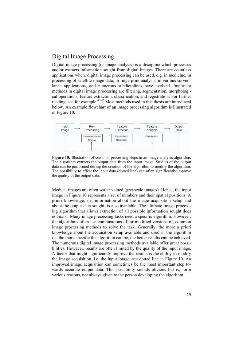
Digital Image Processing Digital image processing (or image analysis) is a discipline which processes and/or extracts information sought from digital images. There are countless applications where digital image processing can be used, e.g. in medicine, in processing of satellite image data, in fingerprint analysis, in various surveil-lance applications, and numerous subdiciplines have evolved. Important methods in digital image processing are filtering, segmentation, morphologi-cal operations, feature extraction, classification, and registration. For further reading, see for example.40-42 Most methods used in this thesis are introduced below. An example flowchart of an image processing algorithm is illustrated in Figure 10.

Figure 10: Illustration of common processing steps in an image analysis algorithm. The algorithm extracts the output data from the input image. Studies of the output data can be performed during the creation of the algorithm to modify the algorithm. The possibility to affect the input data (dotted line) can often significantly improve the quality of the output data.

Medical images are often scalar valued (greyscale images). Hence, the input image in Figure 10 represents a set of numbers and their spatial positions. A priori knowledge, i.e. information about the image acquisition setup and about the output data sought, is also available. The ultimate image process-ing algorithm that allows extraction of all possible information sought does not exist. Many image processing tasks need a specific algorithm. However, the algorithms often use combinations of, or modified versions of, common image processing methods to solve the task. Generally, the more a priori knowledge about the acquisition setup available and used in the algorithm i.e. the more specific the algorithm can be, the better results can be achieved. The numerous digital image processing methods available offer great possi-bilities. However, results are often limited by the quality of the input image. A factor that might significantly improve the results is the ability to modify the image acquisition, i.e. the input image, see dotted line in Figure 10. An improved image acquisition can sometimes be the most important step to-wards accurate output data. This possibility sounds obvious but is, form various reasons, not always given to the person developing the algorithm.

30

FilteringFiltering of image data is sometimes performed as a pre-processing step. The purpose of the filtering might for example be noise suppression or enhance-ment/retrieval of image gradient information. The filtering can for example be performed in the spatial domain or in the frequency domain. Spatial do-main filters use a filter mask (also known as window, kernel or template) consisting of a set of spatially distributed weights. The filtering is performed by spatially traversing the image data (usually pixel by pixel in the 2D case) and multiplying the pixel values by the corresponding filter weights. The result from the filtering gives a new image. The result can be modified by varying the weights and their spatial distribution. The filter mask used can have equal or lower dimensionality than the input image data. One motiva-tion for the use of a mask with lower dimensionality can be the image reso-lution. 3D MR data for example commonly has a higher in-plane resolution. In paper III the gradient filter creating I5-GRAD was for this reason two-dimensional. Examples of filters applied on a binary image are shown in Figure 11.

Figure 11: Filtering examples. a) Binary input image including randomly distrib-uted noise. b-d) Result from application of a median, a mean, and a Gaussian smoothing filter, respectively.

31

Binary Morphology Binary morphology can be used to process and analyse binary images. The binary images are considered to contain one or more objects and back-ground. Commonly the objects are represented by a value greater than zero and the background by the value zero. Examples of tools that can be used to process such images are dilation, erosion, distance transform, and skeletoni-zation.40 Morphological operations are also available for greyscale images. However, these tools have not been used in this thesis.

Binary Dilation and Erosion Dilation and erosion are two commonly used binary morphological opera-tions. These operations affect the objects in image (A) using a structuring element (S). Figure 12 defines and illustrates results from binary dilation, erosion, and combinations of these operations.

Figure 12: Illustration of binary morphology. A is the input image, S is the structur-ing element used. S is composed of a neighbourhood of five pixels. Note that A and S are scaled differently. Definitions and results are given for dilation, erosion, clos-ing, opening, and two operation combinations.

32

Segmentation Image segmentation is often an important step in digital image processing. Segmentation of nontrivial images has been referred to as one of the most difficult tasks in digital image processing.40 The segmentation performs a subdivision of the image data into regions (objects). The problem given de-termines the level to which the image data needs to be segmented. A wide variety of methods can be used. Examples of commonly used methods are: intensity thresholding, morphological operations, region growing, and de-formable models. Combinations of these segmentation methods can also be used. Here follows brief explanations of two of the segmentation methods used in this thesis.

Intensity Thresholding Image segmentation using intensity thresholding has a central role in digital image processing. This is likely because of its simple implementation and intuitive effect on the data. The process of thresholding a grey-level image, f(x,y), using a global threshold T is defined in Equation III.

01

),( yxgTyxfTyxf

),(),(

(III)

Equation III defines a global thresholding operation where g(x,y) is the re-sulting binary image. Image elements with grey values greater that the threshold T result in elements of value 1 in g(x,y). Image elements with grey values smaller or equal to the threshold T result in elements of value 0 in g(x,y). The thresholding operation can also be performed to threshold a ranges of intensities using multiple thresholds. Automated methods can be used to determine the threshold values.43 Automated determinations of thresholds were used in papers I-III.

Region Growing Region growing can be used to emphasize the connectivity or “hanging to-getherness” of objects. The method uses one or more seed points (starting locations) which can be set manually or automatically. The seed points are considered to be an initial segmentation of the object/s. An iterative algo-rithm investigates the neighbourhood of each already segmented object and expands the object as long as a criterion is met. The criterion might for ex-ample be based on image intensity or image gradient information. Region growing that used intensity based criterions were used in papers I-III.

33

Evaluation of Segmentation Results When evaluating the accuracy of segmentation results a reference is needed. The reference can either be created using data from phantom scans, synthetic data, or using manual delineation of the real image data.

Data acquired from phantoms and synthetic data allow assessment of true accuracy. However, since conditions will differ, the similarity between the synthetic or phantom data and the acquisition of the real data can always be questioned.

Manual segmentation of medical image data is preferably performed by ex-perienced radiologists. However, this is resource demanding and does not always have the highest priority. Manual segmentation always results in an operator dependent reference. Hence, the reference will only be a surrogate of the “truth” and accuracy assessments using these types of references need to be treated accordingly.

Repeated acquisition and analysis allows assessment of the method repro-ducibility (paper II and III). This approach generates data needed for statisti-cal power calculations and allows reproducibility comparisons between the suggested method and a reference method.

When assessing accuracy it is important to assess both size and location. An algorithm might for example generate the same volumetric result as the ref-erence but from a completely different position. Therefore the use of preci-sion measures like true positive, false positive segmented pixels and methods based on these measures are needed.44 Segmentation precision measures were used in paper I and III.

34

Feature Extraction The extraction of specific information from the image data is denoted feature extraction. Typical features can be based on object size, shape, color, and texture, to name a few. The information of interest might be the feature val-ues directly or decisions made based on the feature information. Commonly multiple feature values are extracted from each object, and put into a vector of n dimensions, a so called feature vector. Each feature vector represents a sample from a feature space of n dimensions. This information can be used to classify objects based on their feature data, i.e. position in the n-dimensional feature space.42

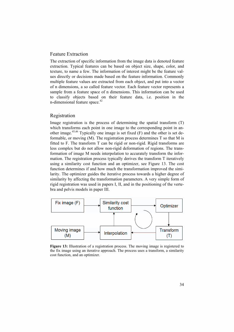
RegistrationImage registration is the process of determining the spatial transform (T) which transforms each point in one image to the corresponding point in an-other image.45,46 Typically one image is set fixed (F) and the other is set de-formable, or moving (M). The registration process determines T so that M is fitted to F. The transform T can be rigid or non-rigid. Rigid transforms are less complex but do not allow non-rigid deformation of regions. The trans-formation of image M needs interpolation to accurately transform the infor-mation. The registration process typically derives the transform T iteratively using a similarity cost function and an optimizer, see Figure 13. The cost function determines if and how much the transformation improved the simi-larity. The optimizer guides the iterative process towards a higher degree of similarity by affecting the transformation parameters. A very simple form of rigid registration was used in papers I, II, and in the positioning of the verte-bra and pelvis models in paper III.

Figure 13: Illustration of a registration process. The moving image is registered to the fix image using an iterative approach. The process uses a transform, a similarity cost function, and an optimizer.

35

Methods in Body Composition Assessment

Analysis of body composition increases the understanding of the complex relationships between body composition and physiological processes stud-ied, e.g. metabolism, in normal as well as in pathological conditions.

For an accurate analysis of body composition, imaging techniques are needed.16,17,47 CT and MRI are considered to give the most accurate results. Both CT and MRI are today widely used for both regional and whole-body analysis of tissue-system level components (see Figure 1). The use of CT exposes the subject to radiation, limiting coverage, longitudinal studies, and studies of children and adolescents. MRI is often the method of choice since it has no known long-term side effects, allows large coverage, repeated ac-quisition, and studies of children and adolescents.

This section first introduces anthropometrical measurements commonly used in analysis of body composition. The use of imaging techniques in body composition is then shortly reviewed with a special focus on the automation of the analysis of MRI data. The section ends with a brief survey of studies comparing body composition assessments from CT, MRI, and DEXA.

36

AnthropometryThe world anthropometry comes from Greek and means “the measurement of humans”. Today anthropometrical measurements such as body mass in-dex, waist circumference, and sagittal abdominal diameter are widely used to monitor medical status of humans.48 These measurements are inexpensive, widely available and portable, hence attractive in field or population based studies.49 However, the results only supply surrogate measures and depend on the skills of the operator.48,50 The accuracy may also vary between popu-lations.48,50-53

Body Mass Index Body mass index (BMI) or “Quetelet’s index” (weight/height2) is a meas-urement that predicts body adiposity (Quetelet, 1869).54 The measurement is simple to perform and BMI forms the back-bone of the obesity classification system, see Table 1. However, BMI gives little insight into regional body fat distribution and it might give misleading information when comparing, for example, groups of different age or ethnicity.51,53 Measurements of BMI were included in all papers and studied in paper IV.

Table 1: BMI classification table.

BMI Classification >30 Obese 25-30 Overweight 18.5-25 Normal <18.5 Underweight

37

Waist and Hip Circumferences Waist circumference (WC), or “waist girth”, and waist-hip-ratio (WHR) are widely used in determination of abdominal adipose tissue and metabolic profile. WC is used as a proxy measure for abdominal obesity and has been shown to correlate better with the metabolic syndrome than fat percentage.55

A large hip circumference seems to have protective effect.56 This might be explained both via the gluteal fat and via the amount of gluteal muscle49

since gluteal muscle might be a good estimate for overall skeletal muscle mass. WHR has for example been shown to predict myocardial infarction better than BMI.49

There are many non-pathologic factors that influence these measurements, thus limiting its use when comparing different populations.52 The measure-ments can be performed at different locations and in either standing or su-pine position thus affecting the results and the possibility of inter-study comparisons. Measurements of WC were included in paper III and studied in two cohorts in paper IV.

Sagittal Abdominal Diameter Sagittal abdominal diameter (sagittal AD/SAD), or “supine abdominal height”, is a strong predictor of VAT57-60 thus also shows strong correlation to markers for obesity related disorders.61-63 Sagittal AD has also been shown to give small inter-observer differences in both lean and overweight sub-jects.50 Studies that measure the sagittal AD compensated for SAT thickness have been performed to enhance the correlation to VAT.57,60,64 Sagittal AD has also been used in combination with DEXA for assessment of VAT.64,65

The use of Sagittal AD was investigated in two cohorts in paper IV.

Transverse Abdominal Diameter Transverse abdominal diameter (transverse AD) is sparsely used in assess-ment of body composition. The use of its predictive value for VAT has been investigated in obese subjects in a study including weight loss59 and in a study combining DEXA and anthropometry.64 Transverse AD can also be used in foetus weight estimation.66 In paper IV transverse AD was found to give information about SAT.

38

Elliptical Approximations Elliptical approximations of cross sectional body areas are seldom used as anthropometrical measurements in studies of body composition. Slice-wise elliptical approximations of abdominal adipose tissue areas have previously been performed with good results using sagittal AD and transverse AD. This has been performed before57,67 and after57,64,67 compensation for SAT thick-ness. An elliptical approximation was studied in paper IV. It was found to strongly correlate with the total amount of adipose tissue (TAT).

Skinfold Thickness Skinfold thickness in combination with predicting equations can be used to measure SAT48,50,68 hence also approximately total body fatness or TAT. SAT thickness can be measured using a calliper or ultrasound (US).60,66 The results from calliper measurements have been reported to depend on the calliper, the operator and the SAT thickness,48,50,68 thus limiting the accuracy. The use of US requires a pressing of a probe against the skin thus this method will likely be highly operator dependent.

39

Computed Tomography The history of the first use of CT in the analysis of body composition is summarized in Table 2.

Table 2: Important methodological body composition studies utilizing CT.

Year Authors Brief study description

1979 Heymsfield et al.69,70 Organ volumes, Skeletal muscle (in arms) 1982 Borkan et al.71 First paper on (IAAT/VAT) assessment 1986 Kvist et al.72/Sjöström et al.73 First whole body AT studies (22 slices)

IAAT – intraabdominal adipose tissue, VAT – visceral adipose tissue, AT – adipose tissue.

CT analysis of body composition has been validated with good results both in humans14,69,74-77 and in animals.78

Heymsfield et al.69 (see Table 2) have investigated the accuracy of organ volume and mass estimations using CT in phantoms, excised human cadaver organs, and organs in situ from two human cadavers. Estimated volumes and masses were found to differ 3 – 5 % from the reference measurements.

Rossner et al.74 have compared CT measurements of adipose tissue from 11 slices of the abdomen, centred on the umbilicus, to planimetry of band sawed slices in two male elderly subjects. High correlations (partial correla-tions of around 0.90) were found.

Body weight estimations in eight males by a whole-body CT based analysis, previously reported by Chowdhury et al.14 and used in paper II, have previ-ously been found to differ very little from real weights, weightCT – weight = 0.024 ± 0.65 kg (standard error = 0.6 kg or 0.85 %). In paper II the weight differences were also found to be non significant (0.40 ± 0.60 kg). In the previous study, interpretation errors calculated from repeated measurement of datasets from four subjects were found to be: TAT, 0.06 L or 0.4 %;

SAT, 0.07 L or 0.5 %; VAT, 0.03 L or 1.2 %; and LUNGS, 0.23 L or 4 %.

Advantages of the use of CT in analysis of body composition are the short acquisition times needed and the absolute Hounsfield numbers given as out-put. CT images also give homogeneous values over the FOV. The dose sub-mitted to the subjects can be significantly reduced by use of dose reduction techniques.79,80 However, dose reduction techniques affect image quality. Very high image quality is however not needed for tissue area and volume determinations using CT. A dose - image quality balancing is nevertheless needed when dose reduction techniques are used.

40

Because of the dose submitted, single slice analysis is the most commonly used method in CT studies.16 However, whole-abdomen investigations do occur.81,82 Since CT numbers from the liver correlate to the degree of liver steatosis one slice can be acquired from the liver to assess liver fat.83,84

Automation of the analysis of body composition using CT is facilitated by the Hounsfield numbers. However, since single slice studies are most com-monly used the need for automation is limited. However, Chowdhury et al.14

have developed a semi-automated software for analysis of 28-slices acquired from subjects in supine position. The current version (2005) of this software was used in Paper II.

41

Magnetic Resonance Imaging MRI is often the method of choice for body composition assessment since it has no known long-term side effects, allows large coverage, repeated acqui-sition and studies of children and adolescents. A very brief history of the use of MRI in studies of body composition is summarized in Table 3.

Table 3: Important methodological body composition studies utilizing MRI.

Year Authors Brief study description

1984 Foster et al.85 SM, AT (Cadaver study) 1988 Hayes et al.86 SAT-thickness (24 males, 26 females, 12 measurement sites) 1991 Fowler et al.87 WB, 28 slices (TAT and SAT in females) 1992 Ross et al.88 WB, 41 slices (SAT, VAT, anthropometric variables) 1998 Thomas et al.17 WB, 3 cm slice gaps, 67 females, subsampling error assessed. 2004 Positano et al.89 Automated SAT and VAT segmentation using snakes. 2006 Liou et al.90 Image analysis algorithm for SAT and VAT segmentation. 2007 Börnert et al.91 WB Dixon method, continuously moving table top

SM – skeletal muscle, AT – adipose tissue, SAT – subcutaneous adipose tissue, WB – whole-body, TAT – total adipose tissue, VAT – visceral adipose tissue.

Analyzed Region Studies of body composition may focus on different sub regions of the body. The abdominal sub region is often of great interest in studies of obesity in-duced health risks. The sub region analyzed affects the choice of image ac-quisition and analysis methods.

Single Slice A single abdominal slice is often the subregion of choice because of the sim-ple acquisition and analysis and because of the relative large amount of in-sight given. However, the slice location used affects the amounts of SAT and VAT measured, hence, also the correlations to the total volumes of SAT and VAT. The locations are commonly referred to by the positions along the spine. (The vertebrae are commonly denoted by T, L, or S and a number. The letters represent thoracic, lumbar, and sacral, and the number denotes the vertebra referred to. For example, L4-L5 denotes the interface between lumbar vertebra 4 and 5.) The umbilicus is also often seen used in the posi-tioning. In the first studies performed the level of L4-L5 was found to con-tain the largest amounts of total adipose tissue.72,87,88,92 Subsequently, many studies used slices positioned at this level. The VAT depot has, in multiple studies, been found more concentrated at higher levels (L2-L3).92-95 How-ever, the slice location with the strongest correlation to the total VAT vol-ume has been found to vary with BMI96 and gender.97 In paper IV analysis of a single MRI slice at the L4-L5 level was used as reference measure.

42

Two studies have investigated the correlation between the location of the analysed slice and obesity-related health risks.93,97 One found that an appro-priately selected single slice VAT area is an equally reliable phenotypic marker of obesity-related health risk as total VAT volume and that the L4-L5 level was not the best marker of obesity-related health risk.97 The other concluded that the VAT area measured was significantly associated with the metabolic syndrome independent of measurements site even though T12-L1, and L1-L2 were found to give stronger correlations than L4-L5.93

Thomas et al.96 have concluded that single-slice MRI appears to be suitable for assessing changes in intra-abdominal fat content in interventional studies, especially in large cohort of subjects, where each subject can serve as its own control. However, for accurate determination of an individual’s intra-abdominal fat content, and inter subject comparison, only multi-slice imag-ing will give precise results.

AbdomenStudies of the whole abdominal region, or multiple slices from it, gives a more robust estimate of adipose tissue depots compared to single slice analy-sis.17,96,98,99 However, a more extensive analysis is required which increases the need for automation of the analysis. In paper III an algorithm for auto-mated segmentation of abdominal data from 16 cm of the abdomen is re-ported.

Whole Body Whole-body assessment of body composition (studied in paper I and II) is motivated by the increased ability for accurate phenotype determinations. Age and ethnicity impacts body composition and studies of these factors likely gain from more extensive analysis. Assessment of redistribution of adipose tissue likely also benefits from whole-body analysis.

A standardized topography that interpolates results from analysis of axial slices, distributed over the whole-body region, based on anatomical positions has been proposed.100 This type of standardization facilitates interpretation and intersubject comparisons.

43

Acquisition Technique MRI acquisition techniques use contiguous or sparse (using inter slice gaps or single slice) data sampling. Sparse data sampling allows reduction of the acquisition and data processing times. Denser data sampling gives more information but increases the time needed for analysis, especially when manual interaction is needed. Denser data sampling increases accuracy and reproducibility and should allow better assessment of regional and longitudi-nal changes, e.g. after intervention. Thomas et al.17 have from whole-body studies of three subjects found that slice gaps approximately give a linear affect on the CV of 1.16 %/cm slice gap. Contiguous data sampling simpli-fies the use of 3D information which might simplify automated segmenta-tion, see papers II and III.

Various techniques are used to acquire and analyze MR data in body compo-sition assessments. Adipose tissue is commonly analysed by use of T1-weighted imaging protocols. However, it has been reported that liver and brain image intensities might overlap the intensities of adipose tissue17,101,102

in these images which complicates the analysis.

Water suppression techniques has been used in multiple studies to suppress the signal intensity from water103-106 and increase the contrast between adi-pose tissue and muscles/organs. However, spectral saturation is dependent on a homogenous magnetic field which is difficult to achieve in large FOVs and inversion recovery sequences used to saturate water are time consuming.

Spectroscopic imaging has been reported in whole-body tissue analysis.107

However, the acquisition time needed and the complicated post processing limits the use in practice.

Whole-body T1-mapping is proposed in papers I and II for automated analy-sis of adipose tissue from whole-body MR data. The technique has been found to simplify automated assessment of adipose tissue (paper I) and the results were found to correlate strongly to results from a well established whole-body CT protocol that utilizes 28 dose-reduced image slices (pa-per II).

Chemical shift imaging (the Dixon method108) can also be used to create water and fat images from acquisition of two or three echoes. This technique also allows quantification of water and fat in tissues and organs.109-112 The long acquisition times of contiguous whole-body data can be reduced using contiguously moving table tops.91,113 A whole-body Dixon acquisition that utilizes a continuously moving table top has been reported. This acquisition technique only requires 2 minutes to generate a whole-body dataset with 6.4 mm isotropic voxels (Table 3).91

44

Data Processing Fully manual data processing, i.e. segmentation methods that use manually determined thresholds and/or manual delineation, is time consuming and operator dependent. In paper III manual segmentation performed by an ex-perienced radiologist was used in order to generate a high quality reference.

Larger coverage, denser sampling, and repeated acquisitions (used for exam-ple in longitudinal studies) demand automation of the data processing. Automation is complicated as MRI image intensity levels are given in arbi-trary units, as images are often affected by intensity inhomogeneities, and as subject sizes and shapes varies significantly.

Compared to manual analysis semi-automated analysis is less time consum-ing and less operator dependent. Semi-automated analysis is therefore com-monly used in assessment of adipose tissue.17,98,100,114 However, it has been concluded that the availability of one experienced operator increases the accuracy.98 T1-weighted images are commonly manually or automatically thresholded on image intensity. Some applications also compensate for im-age intensity inhomogeneities.

Fully automated analysis removes the operator bias and, if accurately per-formed, increases the reproducibility. Fully automated analysis might also reduce the analysis times. Algorithms for automation of the segmentation of subcutaneous and visceral adipose tissue from abdominal data have previ-ously been reported.89,90,104,115,116

Positano et al.89 (Table 3) have presented an automated method for slice-wise analysis of abdominal data using fuzzy c-mean thresholding, snakes, and fitting of a Gaussian function to the adipose tissue histogram peak for segmentation of VAT and SAT. The study presented included 20 subjects and the standard deviations (SDs) of the difference between automated and manual assessments were approximately 16 % and 5.8 % for VAT and SAT, respectively. Even though constraints, not well defined in the paper, were used in the snake algorithm for separation of SAT and VAT it is likely diffi-cult to get good performance for the large variations in abdominal shapes commonly seen.

Liou et al.90 (Table 3) have created a fully automated segmentation method, that has similarities with the algorithm presented in paper III, and measured the performance on image data from four different imaging sequences in 39 overweight/obese (mean BMI = 29) subjects. The algorithm uses common image processing tools for slice-wise data analysis. The algorithm was vali-dated by use of a reference created by using the adipose tissue thresholds

45

determined by the automated algorithm. The SDs of the differences between the automatically derived results and the reference, given as mean values of the four different imaging sequences, were 2.1 % and 0.9 % for VAT and SAT, respectively. Liou et al’s algorithm is seen to be robust to nonstandard cases. However, the algorithm includes steps that limit the use in subjects with normal BMI and resulting segmentations shown in “typical” cases are seen to contain mistakes. The use of the automated threshold, derived by the algorithm, in the creation of the manual reference, and the fact that repeated measurements were acquired from most subjects limits both the use of the validation and the comparison made to the study performed by Positano et al.

Demerath et al.115 have recently published a study that compares two soft-wares that allow VAT and SAT segmentation. Both softwares need manual interaction. They were also reported to give CVs from repeated analysis of whole-abdominal datasets of 4.5 % and 7.3 %, respectively. Average proc-essing times of 60 min and 30 min, respectively, were reported.

A master thesis project on segmentation of abdominal MRI data from males has been reported by Jørgensen et al.116 An active shape model and polar image re-sampling was utilized in the separation of VAT and SAT. The pro-ject report shows visually promising results. Unfortunately, no figures on the accuracy were presented.

Armao et al.104 have published preliminary results on comparisons between semi-automated segmentation of T1-weighted and water-saturated T1-weighted contiguous MR data from the whole abdominal region. Data proc-essing was performed by manual determination of an adipose tissue thresh-old and region growing of the resulting binary objects. No inhomogeneity correction was performed and the thresholding was seen to include the liver in the non-water saturated image data.

Whole-body data acquired using multiple image stacks result in different stack-wise intensity profiles.101,102,117 This affects reconstruction and/or analysis of the whole-body data. Intensity scaling methods have been pro-posed.117 Brennan et al.102 have used histogram matching, though without further specification, in the analysis of whole-body datasets. The whole-body analysis method presented further uses an initial thresholding, boundary enhancement, 3D region growing, a region-refining process with a reference to an algorithm implemented for CT data and with overall little description of the segmentation.

46

Validations Body composition assessed using MRI has been validated with good results both in humans13,47,75,88,92,98,100,118 and in animals.78,119 Multiple MRI valida-tions using human cadavers have been reported.13,47,75

Ross et al.88 (Table 3) have reported differences in TAT measurements of mean 2.9 % (range 0.9 - 4.3 %), for repeated acquisition of three males using a 41-slice whole-body protocol. Ross et al.92 have also reported differences of 1.1 % and 5.5 % for SAT and VAT from repeated single slice acquisitions at the L4 - L5 level in 15 overweight and obese females.

Elbers et al.98 have found CVs for SAT and VAT measurements in nine sub-jects in the BMI range 18.0 - 27.6 kg/m2 to be 0.8 %, 1.8 %, and 8.4 % for TAT, SAT, and VAT, respectively when a single slice at the umbilicus was used. When three neighbouring slices, centred at the umbilicus, were used the CVs were found to be, 0.6 %, 1.6 %, and 5.3 % for TAT, SAT, and VAT, respectively. They conclude that analysis of one slice is sufficient to obtain a reliable estimate of SAT while the use of three slices reduces vari-ability and increases statistical power in measurements of VAT.

Repeated whole-body acquisition and analysis of three subjects, using slices with 1 cm slice gaps, has been demonstrated, by Machann et al.,100 to give differences ranging between 2.0 - 2.7 % and 3.1 - 3.9 % for TAT and VAT, respectively.

47

Dual Energy X-ray Absorptiometry DEXA is commonly used in studies of body composition. Advantages of DEXA usage are the simple acquisition/analysis and the relatively low dose submitted to the subject compared to when CT is used. However, the analy-sis does not allow separation of the visceral and subcutaneous depots. There-fore DEXA is sometimes combined with anthropometrical measurements to assess VAT.64,65

DEXA has been validated in humans,39,120-126 in animals,125-128 and using phantoms.121,126,129,130 DEXA analysis has high accuracy in young healthy subjects.39 However, the method has been reported less accurate in osteo-porotic and obese subjects.39,120,125 The limited accuracy in large subjects is believed to be caused by the thickness of absorber, i.e. the subject.39,122,124-

126,129,130 DEXA inter manufacturer differences have been reported between 0.5 - 6.9 %, 0.4 - 4.4 kg, and 0.3 - 4.1 kg for relative FM, FM, and LTM, respectively.120 Intra manufacturer differences have also been reported.121

The DEXA setup (software version 1.31) used in paper II has previously been validated by Lantz et al.121 Repeated examinations of ten females (BMI 22.1 ± 1.6 kg/m2) gave body fat and lean tissue mass differences of 1.7 % and 0.7 %, respectively.

48

Comparative Studies Studies comparing MRI and CT have previously been performed in ani-mals,78 humans,59,105,131,132 and in human cadavers.47,75 Ross et al78 report that results from MRI and CT analysis of 17 rats correlated strongly. They also found both MRI and CT analysis highly reproducible. In vivo human com-parisons have been performed with varying results in the abdominal re-gion59,105,131 and in the calf.132 Comparisons and validations using cadavers have been performed for measurements of human thighs,75 and skeletal mus-cles in arms and legs.47 To the author’s knowledge paper II is the first whole-body comparison of MRI and CT in assessment of human body composition.

CT and DEXA have previously been compared in body composition analysis of abdomens64,65,133 and legs68,134,135 with good results.

MRI and DEXA have previously been compared in studies of body composi-tion.136-140 A study of VAT measurements from 36 obese subjects (19 fe-males, 17 males) before and after weight reduction has been reported.137

MRI measurements with 4 cm inter slice gaps were used as reference. Weight and BMI were found to estimate the reduction in VAT better than DEXA. It was also concluded that changes in VAT were more difficult to estimate in men than in women. DEXA has also been found to overestimate the amount of TAT by, on average, 17 % compared to 12 slice whole-body MRI at 0.08 T.138

49

SUMMARY OF PAPERS

All studies were performed using volunteer subjects who gave their in-formed consent. The studies were approved by local Ethics Committees. The study in paper II was also approved by a Radiation Committee. All MRI acquisition was performed using a 1.5 T clinical MRI scanner (Gyroscan NT, Philips Medical Systems, Best, The Netherlands) and the body coil.

Paper I – Whole-Body T1-Mapping

AimThe aim of this study was to investigate the feasibility of an acquisition method which was believed to simplify segmentation of adipose tissue from whole-body volumes. The acquisition method is based on T1 quantification and exploits the fact that T1 is shorter in adipose tissue than in other body tissues. T1 was quantified by acquisition of two volumes using two gradient echo sequences with different flip angles; the two flip angles used give tis-sue-dependent variation in image intensity.

MethodsThe study comprised ten volunteer subjects. The whole-body image acquisi-tion was performed using a spoiled T1 weighted gradient echo sequence with TR/TE/slice thickness 177 ms/ 2.3 ms / 8 mm. Axial slices were scanned. Subjects were positioned supine with the arms extended above the head to reduce the maximum patient width. Two whole-body volumes were acquired for each subject using two different flip angles (80 and 30 degrees). The whole-body volumes are denoted Flip80 and Flip30, respectively. Whole-body T1 maps were calculated from each pair of whole-body volumes using the signal equation for a spoiled, steady state, gradient echo sequence.141

Because of limitation of the table top transition, the subjects were imaged in two half-body volumes.

50

The two half-body volumes were registered using a rigid transform (transla-tions in three dimensions) using the ITK142 software package. Adipose tissue was automatically segmented from the T1 maps and from the original Flip80 image slices using thresholding. The thresholds were derived by fitting of two Gaussian curves to slice-wise histogram data. The thresholds were cho-sen as the points of intersection between the two Gaussian curves, see Figure 14c.

The results were evaluated using nine manually segmented slices from the Flip80 volume, from each subject, as reference. The nine slices were chosen to coincide with nine of the slices acquired with the CT scan method de-scribed by Chowdhury et al.14 Adipose tissue pixels were defined as true positive (TP) if they were correctly segmented and false positive (FP) if they were segmented by the automated method but not in the reference. The numbers of TP and FP adipose tissue pixels were counted and compared for total adipose tissue (TAT = SAT + VAT).

In-slice adipose tissue intensity variances in the Flip80 and in the T1-mapped slices were assessed by masking the adipose tissue pixels, manually delineated as adipose tissue in the Flip80 volumes, from both the Flip80 and the T1-mapped volumes. To avoid effects of inter-slice intensity offsets, the mean intensities in the nine Flip80 slice histograms were adjusted to coin-cide with the intensity mean of the whole-body (nine-slice) histogram. This was achieved by adding or subtracting the difference between the means from/to all pixel values. Whole-body (nine-slice) adipose tissue histograms were then constructed from the Flip80 and the T1-mapped data. A Gaussian curve was fitted to every adipose tissue histogram peak using the method of least squares. The SDs of all Gaussian curves were measured.

To investigate the origins of the FP pixels (displayed in red in Figure 15d-e) from both adipose tissue segmentation methods, FP pixels were manually divided by an experienced radiologist into the following classes: SAT in the SAT-skin tissue interface, SAT in other tissue interfaces, VAT, white bone marrow, fat in the intestines, and erroneously segmented adipose tissue, de-noted other. Intermuscular adipose tissue was classified as SAT, and cardiac, thoracic, and intra- and retroperitoneal adipose tissues were classified as VAT. For the classification, the FP pixel positions were shown in the Flip80 images.

The statistical analysis was performed using Student's t-test. P-values <0.01 were considered statistically significant.

51

ResultsThe calculated T1 maps yielded a better histogram separation of adipose tissue (AT) from lean tissue (LT) than the Flip80 volumes, see Figure 14.

Figure 14: The histograms in a) and b) show the number of pixels as a function of arbitrary units (au) and milliseconds (ms) from the Flip80 and the T1-mapped whole-body volumes, respectively. The histogram areas correspond to signals from adipose tissue (AT) and lean tissue (LT). There is good AT separation in the whole-body T1 histogram (b). The inset c) illustrates how the threshold t is chosen as the point of intersection (arrow) between the Gaussian curves fitted to AT and LT, re-spectively.

The SDs of the Gaussian functions fitted to the adipose tissue peaks, ex-pressed as mean (SD), in the Flip80 and the T1-mapped volumes were found to differ significantly, 327(86.4) and 86.9(12.0), respectively (p<0.001).

52

The result from the automatic adipose tissue segmentation in one of the sub-jects is presented in Figure 15. The figure shows the nine analyzed slices from the Flip80 volume, the T1-mapped volume, and the segmented refer-ence volume. It also shows the automated segmentation results from the Flip80 and the T1-mapped volume.

Figure 15: Nine analyzed slices from a), the Flip80 volume, b), the T1-mapped volume, and c), the segmented reference, in one subject. The results from the auto-mated analysis of the Flip80 and the T1-mapped slices are shown in d) and e), re-spectively. In c) the subcutaneous adipose tissue is displayed in bright yellow, vis-ceral adipose tissue in dark yellow, white bone marrow in dark purple, and fat in the intestines in bright purple. In d) and e) true positive values are shown in white, false positive in red and false negative in blue.

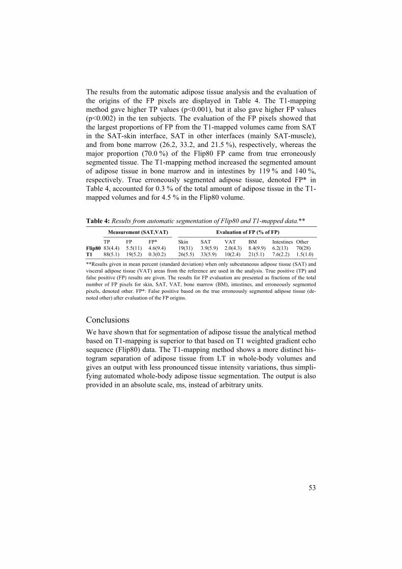
53

The results from the automatic adipose tissue analysis and the evaluation of the origins of the FP pixels are displayed in Table 4. The T1-mapping method gave higher TP values (p<0.001), but it also gave higher FP values (p<0.002) in the ten subjects. The evaluation of the FP pixels showed that the largest proportions of FP from the T1-mapped volumes came from SAT in the SAT-skin interface, SAT in other interfaces (mainly SAT-muscle), and from bone marrow (26.2, 33.2, and 21.5 %), respectively, whereas the major proportion (70.0 %) of the Flip80 FP came from true erroneously segmented tissue. The T1-mapping method increased the segmented amount of adipose tissue in bone marrow and in intestines by 119 % and 140 %, respectively. True erroneously segmented adipose tissue, denoted FP* in Table 4, accounted for 0.3 % of the total amount of adipose tissue in the T1-mapped volumes and for 4.5 % in the Flip80 volume.

Table 4: Results from automatic segmentation of Flip80 and T1-mapped data.**Measurement (SAT,VAT) Evaluation of FP (% of FP)

TP FP FP* Skin SAT VAT BM Intestines Other Flip80 83(4.4) 5.5(11) 4.6(9.4) 19(31) 3.9(5.9) 2.0(4.3) 8.4(9.9) 6.2(13) 70(28) T1 88(5.1) 19(5.2) 0.3(0.2) 26(5.5) 33(5.9) 10(2.4) 21(5.1) 7.6(2.2) 1.5(1.0)

**Results given in mean percent (standard deviation) when only subcutaneous adipose tissue (SAT) and visceral adipose tissue (VAT) areas from the reference are used in the analysis. True positive (TP) and false positive (FP) results are given. The results for FP evaluation are presented as fractions of the total number of FP pixels for skin, SAT, VAT, bone marrow (BM), intestines, and erroneously segmented pixels, denoted other. FP*: False positive based on the true erroneously segmented adipose tissue (de-noted other) after evaluation of the FP origins.

ConclusionsWe have shown that for segmentation of adipose tissue the analytical method based on T1-mapping is superior to that based on T1 weighted gradient echo sequence (Flip80) data. The T1-mapping method shows a more distinct his-togram separation of adipose tissue from LT in whole-body volumes and gives an output with less pronounced tissue intensity variations, thus simpli-fying automated whole-body adipose tissue segmentation. The output is also provided in an absolute scale, ms, instead of arbitrary units.

54

Paper II – Validation of Whole-Body T1-Mapping

AimThis study aimed at validating the use of the MRI based whole-body T1-mapping presented in paper I in body composition studies using a well established 28 slice CT analysis method14 as reference. Whole-body DEXA was also performed. T1-mapping, CT, and DEXA results were compared on a whole-body level as well as on a slice-wise level (MRI and CT only).

MethodsTen volunteers were scanned, using a CT based 28 slice protocol,14 the T1-mapping protocol (paper I), and a DEXA protocol.121 The acquisition of the CT, MRI, and DEXA data from each subject was performed at the same site within a three hour interval. The positioning of the subjects during the CT and the MRI acquisitions was performed as similar as possible to mini-mize inter-modality positioning differences.

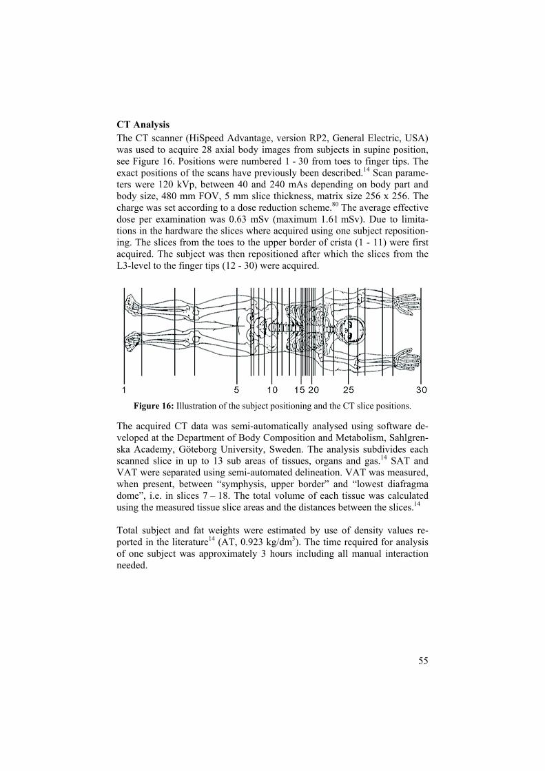
55

CT Analysis The CT scanner (HiSpeed Advantage, version RP2, General Electric, USA) was used to acquire 28 axial body images from subjects in supine position, see Figure 16. Positions were numbered 1 - 30 from toes to finger tips. The exact positions of the scans have previously been described.14 Scan parame-ters were 120 kVp, between 40 and 240 mAs depending on body part and body size, 480 mm FOV, 5 mm slice thickness, matrix size 256 x 256. The charge was set according to a dose reduction scheme.80 The average effective dose per examination was 0.63 mSv (maximum 1.61 mSv). Due to limita-tions in the hardware the slices where acquired using one subject reposition-ing. The slices from the toes to the upper border of crista (1 - 11) were first acquired. The subject was then repositioned after which the slices from the L3-level to the finger tips (12 - 30) were acquired.

Figure 16: Illustration of the subject positioning and the CT slice positions.

The acquired CT data was semi-automatically analysed using software de-veloped at the Department of Body Composition and Metabolism, Sahlgren-ska Academy, Göteborg University, Sweden. The analysis subdivides each scanned slice in up to 13 sub areas of tissues, organs and gas.14 SAT and VAT were separated using semi-automated delineation. VAT was measured, when present, between “symphysis, upper border” and “lowest diafragma dome”, i.e. in slices 7 – 18. The total volume of each tissue was calculated using the measured tissue slice areas and the distances between the slices.14

Total subject and fat weights were estimated by use of density values re-ported in the literature14 (AT, 0.923 kg/dm3). The time required for analysis of one subject was approximately 3 hours including all manual interaction needed.

56

MRI Analysis and Reproducibility The whole-body MRI acquisition is described in paper I.

Fully automated segmentation of bodies and lungs were performed in order to determine the region where the T1-mapped values were of interest. As lung tissue has low signal to noise ratio in the images acquired, the T1-mapped values in the lungs were of limited use. The segmentation of the bodies used a region growing approach combined with two binary whole-body masks denoted Mcrude and Mmin. Mcrude was used to remove motion arte-facts outside the body and Mmin was used to prevent the region growing of the background from penetrating the body. The segmentation of the lungs was performed by use of thresholding, morphological operations, and filter-ing based on object size.

AT was segmented from the T1-mapped data using thresholds derived from the whole-body T1 histograms (see paper I).

SAT and VAT were separated by an experienced radiologist using manual classification. VAT was classified from binary adipose tissue results from the thresholded T1-maps. Flip80 image data was displayed next to the binary adipose tissue results to aid the classification. The total SAT and VAT vol-umes were estimated using the results from the manually classified binary adipose tissue data.

Visual selection of slices 1 – 30 from the continuous whole-body data was performed by an experienced radiologist. The slice selections were per-formed based on congruence in anatomical structures, using the acquired CT slices as reference. The MR slice selections were performed using the Flip80 data and the resulting slice positions were used in the slice-wise evaluation.

The simple thresholding of the T1-mapped data includes bone marrow (BM) in the adipose tissue volumes measured. To assess the effect on the SAT areas measured in the comparison to CT the BM was manually segmented by an experienced operator. Eight slices (2 - 9) were segmented by delinea-tion of BM from the adipose tissue determined using the T1-mapping. The CT images and the Flip80 images were simultaneously visualized to aid the segmentation.

57

Reproducibility of the MRI based T1-mapping was assessed using five sub-jects (three females, two males, BMI mean, 23.0 kg/m2; range 21.3 – 24.3 kg/m2) recruited solely for the purpose of the reproducibility assess-ment. The data was acquired using a scanner software update which allowed stack-wise multi flip angle acquisition between the table top translations. Nine stacks were acquired covering a total of 2.25 m from the subject bod-ies. Repeated acquisition was performed. One whole-body acquisition, in-cluding six breath holds, took approximately 15 minutes.

DEXA Analysis The DEXA scanner used was a LUNAR DPX-L (Lunar Co., Madison WI) with software version 1.35 and an extended analysis program for total body analysis (LUNAR Radiation, Madison WI). Body fat, lean tissue mass, bone mineral content, and weight were assessed.

Statistical Analysis Linear correlations were studied and are reported as correlation coefficients (r-values). Differences were investigated using Wilcoxon signed-rank test. Linear regression analysis was used to study dependencies. P-values <0.05 were considered significant.

58

Results

Whole-Body Comparisons: Correlations, differences, and linear dependencies between CT, MRI based T1-mapping, and DEXA measurements are given in Table 5. Strong correla-tions (r 0.977) were seen for all estimated volumes. The MRI based T1-mapping analysis was seen to overestimate SAT volumes and underesti-mate VAT and total body volumes. Total subjects weights estimated from the CT and the DEXA analysis were not seen to differ from the weights as-sessed by scales. The fat weights estimated from the MRI analysis did not differ significantly from the fat weights estimated by CT. DEXA was found to underestimate the total fat weights compared to CT.

Table 5: Whole-body correlations, differences, and linear dependencies between CT, MRI based T1-mapping (MRI), and DEXA measurements (n=10). Volume comparisons (MRI – CT)Volume Correlation Difference (L) Linear dependence (L)Total 0.998 -2.03 ± 1.61, p=0.005 -0.045CT + 1.920, p=0.054 AT 0.995 -0.61 ± 1.17, p=0.114 -0.004CT – 0.754, p=0.916 SAT 0.977 2.77 ± 2.41, p=0.007 -0.007CT + 2.563, p=0.933 VAT 0.987 -0.79 ± 0.75, p=0.005 -0.209CT + 0.310, p=0.002 Subject weight comparisonsModalities Correlation Difference (kg) CT - Scales 1.000 0.40 ± 0.60, p=0.114 DEXA - Scales 1.000 -0.22 ± 0.42, p=0.114 Fat weight comparisonsModalities Correlation Difference (kg) MRI – CT 0.995 -0.56 ± 1.08, p=0.114 DEXA – CT 0.986 -3.82 ± 1.86, p=0.005 DEXA – MRI 0.979 -4.67 ± 2.38, p=0.005

AT – adipose tissue (SAT + VAT), SAT – subcutaneous adipose tissue, VAT – visceral adi-pose tissue. Correlations are given as correlation coefficients (r-values). Differences are given as mean ± SD.

59

Slice-Wise Comparisons: The results from the slice wise comparison of total area, SAT, and VAT between CT and MRI based T1-mapping are displayed in Figure 17.

Total Body Areas: Total body areas were often underestimated by the MRI based method com-pared to CT, see Figures 17a and 17c. The absolute slice area was underes-timated in 11 slice positions and overestimated in two slice positions. Lin-ear regression showed a significant dependence on slice area (MRI - CT = -0.053CT + 19.1, r=0.584, p<0.0001). The slice positioned at the top of the skull (slice 27) was found to overestimate the area from the MRI based method compared to CT by more than 30 cm2 in eight of the subjects.

Subcutaneous Adipose Tissue Areas: SAT areas were often overestimated by MRI compared to CT, see Figures 17a and 17d. Significant differences were found in 19 slice positions. Slices positioned at the ankle joint, the knee, in pelvis, in thorax, and in the wrists were found to overestimate the SAT area while slices at the L3 level and at the level of the lower orbital border (slices 12 and 25) underestimated the SAT areas. Linear regression on all differences showed a dependence on the SAT area measured by CT (MRI - CT = 0.041CT + 16.7, r=0.161, p<0.0001).

The slice-wise differences in SAT after manual exclusion of BM are shown in Figure 17c (dotted line). Significant differences were seen in 4 slice posi-tions (compared to 5 before exclusion of BM). SAT was overestimated in slices at the symphysis lower border and acetabulum upper border (6 and 8) after exclusion of BM while the slices at the ankle joint and calf (2 and 3) were underestimated after the exclusion of BM. The absolute differences, in SAT areas measured, between MRI and CT were significantly reduced in slices (2, 4, 6-9) by the exclusion of BM.

Visceral Adipose Tissue Areas: Figures 17a and 17e show that VAT areas often were underestimated by MRI compared to CT. Significant differences were seen in 8 slice positions. Slices between upper border of the acetabulum and the L1 level (8-13) and at the positions of the lowest diafragma dome and 7 mm above this position (16, 17) were underestimated by MRI compared to CT. Linear regression on all differences showed a dependence on the VAT area measured by CT (MRI - CT = -0.155CT - 0.459, r=0.575, p<0.0001).

60

Figure 17: Results from slice-wice comparison between MRI based T1-mapping (MRI) and CT. a) Slice-wise mean total body, subcutaneous adipose tissue (SAT), and visceral adipose tissue (VAT) slice areas from CT and MRI. B) Illustration of the 30 slice positions. c-e) Slice-wise differences (MRI – CT), given as mean ± confidence interval, for total area, SAT, and VAT, respectively. In d), the mean SAT values, after exclusion of bone marrow (BM), are given for the eight slices (dotted line).

61

The reproducibility of the MRI based T1-mapping gave absolute differences in total body, total adipose tissue, and segmented lung volumes of (mean ± SD) 0.21 ± 0.15 %, 3.3 ± 3.3 %, 3.2 ± 3.3 %, respectively.

ConclusionsWe have shown strong correlations between body composition analysis re-sults in whole-body regions from CT, MRI based T1-mapping, and DEXA. If the differences between the results from T1-mapping and from the CT based analysis are accepted the T1-mapping protocol allows a fully auto-mated post processing of whole-body MR data allowing longitudinal whole-body studies also applicable in children and adolescence.

62

Paper III – Automated VAT and SAT segmentation

AimThis study had two objectives. 1) To develop a fully automated algorithm for segmentation of VAT and SAT, excluding intermuscular adipose tissue and bone marrow, from axial abdominal MRI data. 2) To evaluate the algorithm accuracy and total method reproducibility by use of a manually segmented reference and data from repeated measurements.

Methods

SubjectsTwo cohorts were used in this study. The first consisted of 13 subjects (6 females, 7 males) and was denoted the derivation cohort and the other con-sisted of 18 subjects (6 females, 12 males) and was denoted the validation cohort.

MRI Acquisition The MRI acquisition was performed using a T1 weighted 2D multislice spoiled gradient echo acquisition of 16 contiguous axial slices of the abdo-men. The volume was centered over L4-L5 and acquired in one breath hold. The slices acquired are hereafter denoted 1-16 from caudal to cranial. The volumes acquired included the arms of the subjects. To simplify the auto-mated image processing careful subject positioning was used to ensure that the arms of the subjects were separated from the abdomen in all image slices. The scan parameters used were TR/TE/Flip, 129 ms / 4.6 ms / 80 degrees, and FOV/Matrix/slice thickness, 430 mm / 256 / 10 mm. Ante-rior-posterior phase coding direction was used. Scan time was 16 s. Repeated measurements were acquired from all subjects in the validation cohort.

63

Automated Segmentation Algorithm The automated image analysis was performed using a standard set of image processing tools40 such as thresholding, compensation for intensity inho-mogeneities, morphological operators and a priori geometrical models. The algorithm was implemented in C++ and the ITK142 software package was used for the basic data processing and handling. The aim of the algorithm was robust segmentation of VAT and SAT excluding inter-/intramuscular adipose tissue and bone marrow. No user interaction is required during the execution of the algorithm and the segmented image data and volume results are given as output.

The algorithm uses following tools, which are described in more detail in paper III, appendix A: The connected area mapping (CAM) tool is used to analyse objects based on in-slice connectedness. The Connected Volume Mapping (CVM) tool is the extension of the CAM tool utilized for con-nected volume analysis in 3D. The orthogonal convex hull tool is an adapted version of a convex hull.40 The pelvis and vertebra models are geometrical models of the pelvis and the vertebral region used to include geometrical a priori information.

Notations:I – Grey level images B – Binary images T – Threshold levels H – Histograms G – Gaussian functions

Subscripts ISTEP,EVENT/DESCRIPTION are used to identify where an object is cre-ated or used. Step defines step (1-8) according to the definition below and event/description is used to further specify the use.

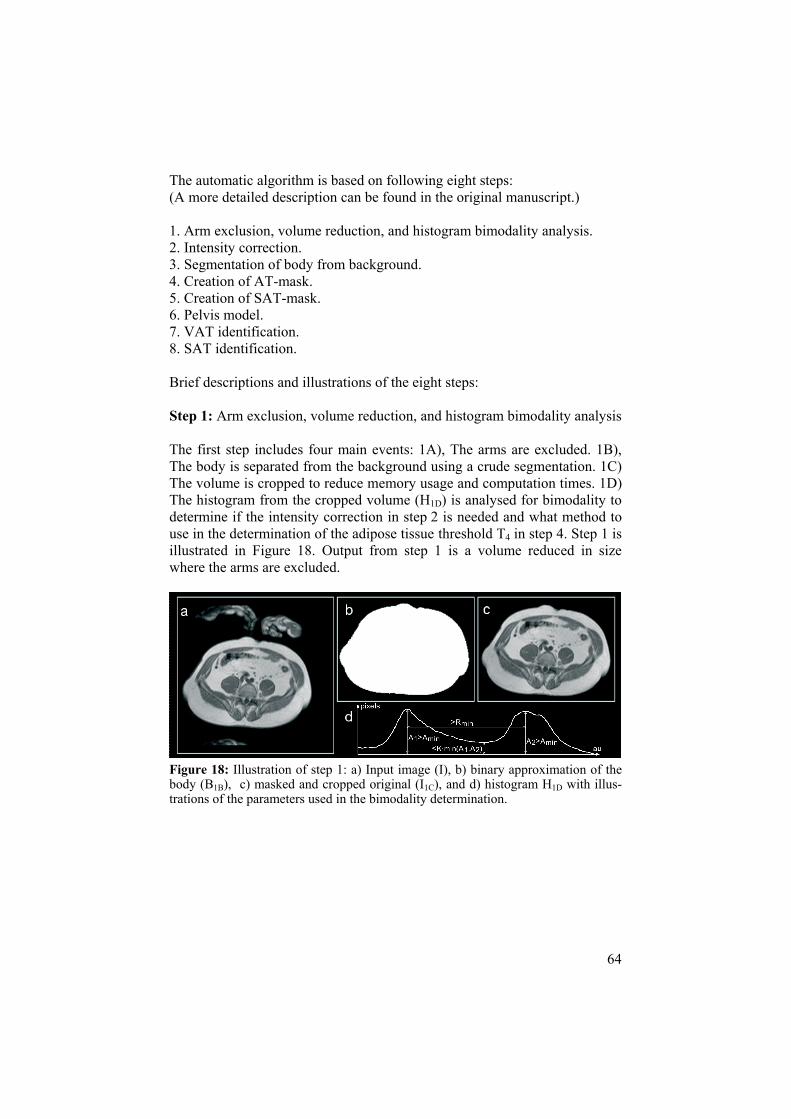
64

The automatic algorithm is based on following eight steps: (A more detailed description can be found in the original manuscript.)

1. Arm exclusion, volume reduction, and histogram bimodality analysis. 2. Intensity correction. 3. Segmentation of body from background. 4. Creation of AT-mask. 5. Creation of SAT-mask. 6. Pelvis model. 7. VAT identification. 8. SAT identification.

Brief descriptions and illustrations of the eight steps:

Step 1: Arm exclusion, volume reduction, and histogram bimodality analysis

The first step includes four main events: 1A), The arms are excluded. 1B), The body is separated from the background using a crude segmentation. 1C) The volume is cropped to reduce memory usage and computation times. 1D) The histogram from the cropped volume (H1D) is analysed for bimodality to determine if the intensity correction in step 2 is needed and what method to use in the determination of the adipose tissue threshold T4 in step 4. Step 1 is illustrated in Figure 18. Output from step 1 is a volume reduced in size where the arms are excluded.

Figure 18: Illustration of step 1: a) Input image (I), b) binary approximation of the body (B1B), c) masked and cropped original (I1C), and d) histogram H1D with illus-trations of the parameters used in the bimodality determination.

65

Step 2: Intensity correction

Intensity correction is performed to reduce the effects of image intensity inhomogeneities caused by the non-optimal static, radio frequency, and gra-dient fields. From prior experience and from the analysis of the derivation cohort it was concluded that the intensity correction is not needed when ana-lysing small subjects. The method used also gives better correction results on subjects with more adipose tissue; therefore, intensity correction is not per-formed on datasets that show a non bimodal H1D-histogram. Step 2 includes three main events, 2A-C. In 2A) pixels that contain adipose tissue are deter-mined. In 2B) polynomials are slice-wise fitted to the intensities of the pixels containing adipose tissue, see illustration in Figure 19. In 2C) the compensa-tion is performed slice-wise using the polynomial approximations. Output from step 2 is a volume with reduced or small adipose tissue image intensity inhomogeneities.

Figure 19: Illustration of the fitting of the second order surface, in grey, to the adi-pose tissue pixels, in white. Note that an offset in z-direction is added to improve simultaneous visualization.

66

Step 3: Segmentation of body from background

The segmentation of the body is performed using a region growing of the background until an automatically determined threshold intensity value is reached. The threshold is determined using only pixels in a border region covering mainly background, skin, and SAT. This method is independent of what is inside the border region i.e. the amount of adipose tissue, intestines, muscle, or liver. This is advantageous since pixel values inside this region do not aid the body threshold determination. Step 3 consists of three main events, 3A-C. In 3A) a mask covering the border region of the body is cre-ated. In 3B) a histogram is created from pixels in the border region and in 3C) the threshold is determined. Step 3 is illustrated in Figure 20. Output from step 3 is a binary volume of the abdominal region (B3C) and the volume image (I3C) masked by the binary volume.

Figure 20: Illustration of step 3: a) Input image (I2C), b) binary border mask (B3A), and c) the masked border pixels and their histogram. The arrow depicts the calcu-lated body threshold (T3).

67

Step 4: Creation of AT-mask

The automated determination of the adipose tissue threshold T4 is performed using one of two methods, depending on the shape of the H1D histogram. Both methods analyse the histogram H4 derived from pixel data in the vol-ume image (I3C) created in step 3. T4 allows creation of the thresholded vol-ume image B4-AT which estimates pixels that mainly contain adipose tissue. These pixels are hereafter denoted AT-pixels. A B4-REST image is created from the object pixels in B3C that are not present in B4-AT. B4-REST determines the pixels mainly containing non-fatty tissue i.e. muscle, bone, organs, and intestines. These pixels are hereafter denoted non-fat-pixels. Step 4 is illus-trated in Figure 21. Outputs from step 4 are the binary images B4-AT and B4-

REST.

Figure 21: Illustration of the AT thresholding using T4. a) The input image (I3C), the thresholded AT-pixels (B4-AT), and the non-fat-pixels (B4-REST) inside the body.

68

Step 5: Creation of SAT-mask

The purpose of this step is to create a SAT-mask, B5, which separates SAT from other tissues. The creation of B5 is described using three main events, 5A-C. In 5A) a gradient magnitude image is computed (I5-GRAD). In 5B) a mask, B5-GRAD, is created from I5-GRAD. In 5C) B4-REST is masked using B5-GRAD to remove non-fat-pixels in the SAT region and create B5. The SAT-mask B5 is used to separate B4 into B5-VAT and B5-SAT. Step 5 is illustrated in Figure 22. Outputs from step 5 are the binary mask B5 and the binary images B5-VAT and B5-SAT.

Figure 22: Illustration of step 5: Creation of a mask (B5) that separates SAT from the rest. a) Input image (I3C), b) B4-REST illustrating erroneously segmented non-fat-pixels that need to be removed, c) gradient magnitude image (I5-GRAD) masked using a slice-wise eroded copy of B3C, d) I5-GRAD after thresholding, e) the mask (B5-

COARSE) superimposed in dark on the input image (I3C). In f) B5C is shown and g) and h) show the B5-mask.

69

Step 6: Pelvis model

Bone marrow sometimes gives high signal intensity areas in the images ac-quired resulting in AT-pixels in B5-VAT. In this study, neither bone marrow, nor inter-/intramuscular adipose tissue is of interest. The number of pixels segmented as adipose tissue in B5-VAT from these compartments is reduced by locally raising the T4 threshold (T4-LOCAL). That is, regions with a high probability of containing bone marrow, and adipose tissue depots of low interest in this study, are thresholded using the higher threshold. The regions where this is performed are determined by the pelvis model. Step 6 is per-formed using two main events, 6A and 6B. In 6A) the pelvis model is posi-tioned in the volume using automated finding of the spinal cord position. In 6B) the T4-LOCAL threshold is applied to reduce the contribution from fat de-pots of no interest in this study. Step 6 is illustrated in Figure 23. Output from step 6 is a binary image (B6-VAT) containing reduced amounts of bone marrow and inter- /intramuscular adipose tissue segmented as adipose tissue.

Figure 23: Single slice illustration of the pelvis model in use. a) AT-pixels within the B5 mask (B5-VAT), b) highlighted area illustrates the region anterior to the pelvis model, and c) the result (B6-VAT) after the adipose tissue threshold is raised posterior to the pelvis model (T4-LOCAL).

70

Step 7: VAT identification.

The identification of VAT-pixels from B6-VAT is performed using four main events, 7A-D. In 7A), the vertebra model is used to remove unwanted binary objects from B6-VAT. In 7B), a region growing is performed to extend the VAT depot. In, 7C) small connected objects in B6-VAT are removed. In 7D), a mask (B7) covering the VAT region is created and used to undo incorrect deletions of small connected VAT objects removed in event 7B). Step 7 is illustrated in Figure 24. Outputs from step 7 are the final binary image con-taining the VAT pixels and a binary image (B7) that covers the visceral re-gion.

Figure 24: Illustration of step 7: a) shows the pixels in B6-VAT and the striped region shows one slice of the vertebra model used to include geometrical a priori knowl-edge. In b), B7C from the same slice is shown. In c) the union of B7C and B7D is shown and B7 is shown in d).

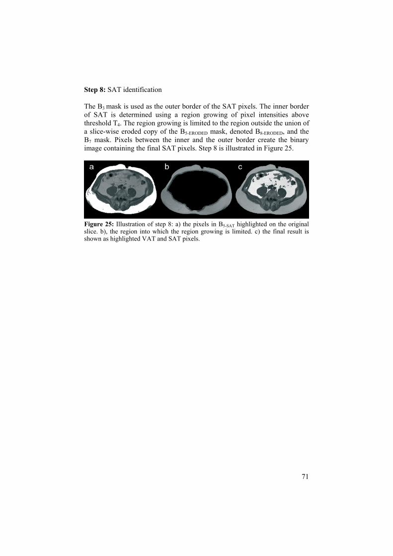
71

Step 8: SAT identification

The B3 mask is used as the outer border of the SAT pixels. The inner border of SAT is determined using a region growing of pixel intensities above threshold T4. The region growing is limited to the region outside the union of a slice-wise eroded copy of the B5-ERODED mask, denoted B8-ERODED, and the B7 mask. Pixels between the inner and the outer border create the binary image containing the final SAT pixels. Step 8 is illustrated in Figure 25.

Figure 25: Illustration of step 8: a) the pixels in B5-SAT highlighted on the original slice. b), the region into which the region growing is limited. c) the final result is shown as highlighted VAT and SAT pixels.

72

EvaluationThe evaluation of the automated algorithm was performed assessing accu-racy and reproducibility. The accuracy was assessed using a, by an experi-enced radiologist, manually segmented reference where adipose tissue pixels from intestines were excluded and inhomogeneities were compensated for. The reproducibility of the manual analysis was assessed using a less exten-sive and more commonly used approach, without the manual exclusion of adipose tissue pixels from intestines and without the manual compensation for inhomogeneities.

The creation of a reference of this accuracy was labor intense. The accuracy was therefore only assessed using every second slice (2, 4…). The accuracy was measured by absolute and relative differences of VAT and SAT vol-umes derived from the fully automated and the manual analysis, respectively and by calculating the fractions of true positive (TP) and false positive (FP) segmented pixels using the manually segmented data as reference.

Reproducibility, including both acquisition and analysis differences, was assessed using the repeated measurements from the evaluation cohort. The relative difference of the VAT and SAT volumes measured using the fully automated segmentation algorithm and the results from manual analysis were calculated. The manual analysis of the reproducibility data was per-formed by two experienced radiologists (1 and 2) and two experienced op-erators (3 and 4) who manually segmented adipose tissue from all image slices using volume-wise intensity thresholding. The adipose tissue pixels were manually separated into VAT and SAT. Adipose tissue pixels originat-ing from bone marrow, inter- and intramuscular adipose tissue were manu-ally removed. Pixels thresholded as adipose tissue originating from intestines were not removed and no manual corrections were performed.

The statistical analysis was performed using the software StatView (SAS Institute Inc. Cary, NC, USA. www.statview.com). Student’s paired t-test was used to test for significant differences between automated and reference VAT and SAT measurements and between TP and FP fractions from VAT and SAT, respectively. The F-test was used to test variance differences. P-values < 0.05 were considered statistically significant.

73

ResultsThe results from accuracy and reproducibility measurements from 17 of the 18 subjects in the validation cohort are shown in Table 6. One athletic male subject was found to have very little adipose tissue and was therefore con-sidered to be an outlier. No significant absolute or relative accuracy differ-ences between automated analysis and the reference were found.

Table 6: Segmentation accuracy and reproducibility in validation cohort (n=17).*

AccuracyReproducibility

(Meas1 – Meas2)/Meas1

Auto-Ref (cm3)

Auto-Ref(%)

TP / FP (%)

Auto(%)

Man 1(%)

Man 2(%)

Man 3(%)

Man 4 (%)

VAT -2.5±80 2.0±14 90±6.5 / 12±12 0.24±7.1 5.1±12 3.4±16 7.3±19 -0.39±13 SAT -8.1±35 0.84±2.7 96±2.3 / 3.6±1.0 0.21±2.3 0.78±3.7 1.2±3.8 1.6±4.1 0.29±4.3

*Data is given as mean value ± standard deviation. Auto – Results from automated analysis. Ref – Results from reference measurement. Note that the accuracy data is based on the even slices in each volume. Meas1/Meas2 – First and second reproducibility measurement (including repeated acquisition and analy-sis). Man (1-4) – Manual measurements by operator 1-4.

TP values were seen higher for SAT than for VAT (p=0.0011) and were seen to vary less for SAT than for VAT (p<0.0001). FP values were significantly larger for VAT than for SAT (p=0.0040) and the variance was significantly higher for VAT than for SAT (p<0.0001).

The reproducibility measurements showed that the fully automated analysis gave a lower variance for the VAT measurements (p<0.029) and for the SAT measurements (p<0.037) than what the manual approach did.

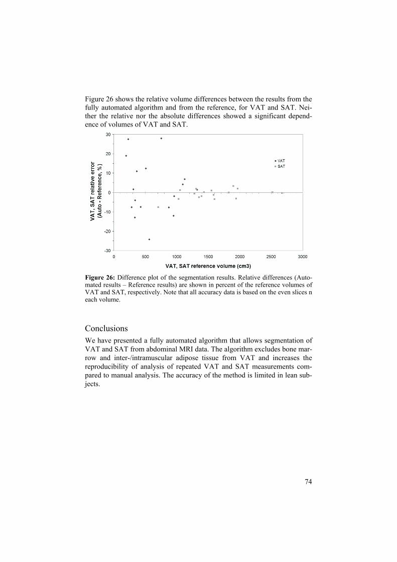
74

Figure 26 shows the relative volume differences between the results from the fully automated algorithm and from the reference, for VAT and SAT. Nei-ther the relative nor the absolute differences showed a significant depend-ence of volumes of VAT and SAT.

Figure 26: Difference plot of the segmentation results. Relative differences (Auto-mated results – Reference results) are shown in percent of the reference volumes of VAT and SAT, respectively. Note that all accuracy data is based on the even slices n each volume.

ConclusionsWe have presented a fully automated algorithm that allows segmentation of VAT and SAT from abdominal MRI data. The algorithm excludes bone mar-row and inter-/intramuscular adipose tissue from VAT and increases the reproducibility of analysis of repeated VAT and SAT measurements com-pared to manual analysis. The accuracy of the method is limited in lean sub-jects.

75

Paper IV – Abdominal Diameters

AimThis study had two objectives. 1) To investigate the correlations between anthropometrical measurements, VAT and SAT in two cohorts differing in age using MRI as reference. 2) To investigate the potential usage of abdomi-nal diameters in practical estimation of adipose tissue compartments using these cohorts.

Methods

Subjects and Anthropometrical Measurements The first cohort contained 306 subjects of age 70 who volunteered to partici-pate in the Prospective Investigation of the Vasculature in Uppsala Seniors (PIVUS) study.143 The other cohort contained 50 volunteers of mixed ages between 14 and 66 years. The cohorts are denoted the cohort of elderly and the mixed younger cohort, respectively.

Anthropometrical measurements (weight, height, and WC) were collected using standardized equipment and procedures. Sagittal abdominal diameter (sagittal AD, or SAD) and transverse abdominal diameter (transverse AD, or TAD) were measured from MR images and were considered to be surrogate anthropometrical measurements.

MRI Acquisition and Image Analysis The acquisition of the cohort of elderly was performed using a steady state free precession sequence. The same sequence was used for the purpose of acquiring a whole-body survey of the subject. The scan parameters used were TR/TE/flip, 3.2 ms/1.6 ms/50°, and FOV/matrix/slice thickness, 450 mm/256/10 mm. The acquisition of the mixed younger cohort was per-formed using a spoiled gradient echo sequence. The scan parameters were TR/TE/flip, 129 ms/4.6 ms/80°, and FOV/matrix/slice thickness, 430 mm/256/10 mm.

76

The segmentation of SAT and VAT was performed manually by two experi-enced operators. A single slice, at the L4-L5 interface, from each subject was segmented. The data from the cohort of elderly was segmented by operator one and from the mixed younger cohort by operator two. In order to deter-mine the variability introduced by the operators the inter- and intra-observer variability for SAT and VAT measurements were assessed by repeated analysis of 20 randomly selected subjects from the cohort of elderly. The intra-observer investigation was performed by operator two and the meas-urements were separated in time by one week.

The sagittal AD was defined as the largest spanned height, in anterior-posterior direction, of the body in the imaged slice, see Figure 27. Trans-verse AD was defined as the largest spanned width of the body in the imaged slice, see Figure 27. The diameters were measured by manual fitting of the smallest possible rectangular object including the whole abdominal area in each analysed slice. The use of an elliptical assumption of the abdominal shape in axial images has previously been demonstrated in prediction of abdominal adipose tissue.57,64,67 Therefore, the calculated area of the ellipse spanned by the sagittal and transverse abdominal diameters (i.e. the largest possible ellipse inside the rectangle, see Figure 27) was used to estimate TAT (TAT = SAT + VAT).

Figure 27: Illustration of the diameters measured and the elliptical approximation made. SAD – sagittal abdominal diameter, TAD – transverse abdominal diameter. Subcutaneous and visceral adipose tissues are displayed in light grey and grey, re-spectively.

There were time intervals between the anthropometrical measurements (BMI and WC) and the images acquired (Sagittal AD, Transverse AD, ellipse, SAT, VAT, and TAT). The cohort of elderly was examined using MRI on average 16 months (range from 3 to 24 months) after the anthropometrical measurements were performed. The mixed younger cohort was examined using MRI on average 4 months (range from 0 – 7 months) before the an-thropometrical measurements were performed.

77

Statistical Analysis Linear correlation coefficients between the abdominal adipose tissue com-partments (TAT, SAT, and VAT) and the true and surrogate anthropometri-cal measurements (BMI, WC, sagittal AD, transverse AD, and ellipse area) were calculated. Correlations were calculated for gender specific groups for both cohorts studied. Fisher’s z-transformation and t-tests were used in de-terminations of correlation significances and in tests on correlation differ-ences. The correlation between age and the different regression residuals were studied using linear regression. P-values <0.05 were considered signifi-cant.

Multiple regression models for TAT, SAT, and VAT were created using the whole study material to determine the strongest independent contributions to the model. The models were created using backward elimination and P-values <0.05 were used to determine factors contributing significantly to the models.

78

ResultsResulting correlation coefficients between the anthropometrical measure-ments and the adipose tissue areas measured from the single slice MRI analysis are given for the cohort of elderly and for the mixed younger cohort in Tables 7 and 8, respectively. The anthropometrical measurements showed, on average, 19 % and 14 % stronger correlation coefficients for TAT and SAT, respectively, than for VAT, in the cohort of elderly. A trend was that the correlations were stronger in the mixed younger cohort than in the cohort of elderly (22 out of 30 correlation coefficients were slightly stronger and five were significantly stronger in the mixed younger cohort). Sagittal AD gave the strongest correlation to VAT (significant in three out of four cases). Transverse AD showed significantly stronger correlations to SAT than to VAT in all subject groups except for males in the mixed younger cohort. The elliptical approximation showed an overall very strong correlation to TAT (r 0.962).

Table 7: Correlations between anthropometric measurements and the amount of adipose tissue measured from the single slice MRI analysis in the cohort of elderly.*

Females (n=138) Males (n=148)TAT SAT VAT TAT SAT VAT

BMI 0.841 0.795 0.641 0.852 0.795 0.735 WCa 0.859 0.790 0.700 0.855 0.776 0.765 SADb 0.925 0.839 0.780 0.941 0.848 0.848 TADb 0.917 0.914 0.598 0.917 0.872 0.767 Ellipseb 0.968 0.918 0.731 0.962 0.885 0.844 *TAT – total adipose tissue, SAT – subcutaneous adipose tissue, VAT – visceral adipose tissue, BMI – body mass index, WC – waist circumference, SAD – sagittal abdominal diame-ter, TAD – transverse abdominal diameter. All correlations were significant with P<0.0001. a Measurements missing in one female and four males. b Note that the abdominal diameters were assessed using MRI.

Table 8: Correlations between anthropometric measurements and the amount of adipose tissue measured from the single slice MRI analysis in the mixed younger cohort.*

Females (n=23) Males (n=27)TAT SAT VAT TAT SAT VAT

BMIa 0.912 0.879 0.869 0.916 0.888 0.749 WC 0.920 0.926 0.794 0.953 0.838 0.868 SADb 0.954 0.890 0.970 0.958 0.818 0.904 TADb 0.917 0.947 0.740 0.941 0.866 0.807 Ellipseb 0.980 0.955 0.913 0.979 0.848 0.908 *TAT – total adipose tissue, SAT – subcutaneous adipose tissue, VAT – visceral adipose tissue, BMI – body mass index, WC – waist circumference, SAD – sagittal abdominal diame-ter, TAD – transverse abdominal diameter. All correlations were significant with P<0.0001. a Measurements missing in one male. b Note that the abdominal diameters were assessed using MRI.

79

The results from the multiple regression models created using the whole study material are given in Table 9. The results illustrate the usefulness of the abdominal diameters and the importance of age and gender in studies of anthropometry. The time interval between the anthropometrical measure-ments and the image acquisitions and the measurements of TAD and SAD from the images likely affect the models. Note that the TAT-model not in-cludes BMI, nor WC and that the VAT-model indirectly includes SAD via TAD(-) and ellipse(+).

Table 9: Multiple regression table. The significant factors, ordered after decreasing absolute t-values. (+/- for positive or negative model contribution).*

Model Significant model factors

TAT Ellipse (+), subject height (-), gender (+), age (-), and TAD (+). SAT Ellipse (+), TAD (+), age (-), gender (+), and subject height (-). VAT TAD (-), ellipse (+), age (+),WC (+), SAD (+), subject height (-), and BMI (-) *TAT – total adipose tissue, SAT – subcutaneous adipose tissue, VAT – visceral adipose tissue, Ellipse – ellipse area, gender – (female = 1, male = 0), TAD – transverse abdominal diameter, WC – waist circumference.

The average coefficients of variation (CVs) from repeated measurements in 20 randomly selected slices were 1.4 % and 3.2 % for SAT and VAT, re-spectively. The inter-operator average CVs from measurements of the same slices were 3.4 % and 5.9 % for SAT and VAT, respectively.

ConclusionsWe have shown that sagittal and transverse abdominal diameters assessed using MRI show strong correlations to VAT and SAT, respectively. These results suggest the use of abdominal diameters in practical estimations of VAT and SAT depots.

80

DISCUSSION

In this thesis MRI has been used in assessment of whole-body (paper I-II) and regional (paper III) adiposity. MRI has also been used as reference in evaluation of anthropometrical measurements (paper IV).

VAT has been treated as one depot, without the separation into intra- and extraperitoneal adipose tissue,6 neither has SAT been separated into superfi-cial and deep SAT.6 These separations might be of medical interest.6 How-ever, fully automated separation into these sub depots are likely very diffi-cult to achieve and semi-automated analysis is most likely needed. Chemical shift imaging, parallel imaging, and imaging at 3T can also be of interest in future studies of body composition assessment.

The whole-body acquisition and analysis method proposed in papers I and II allows fully automated post processing for assessment of total amount of adipose tissue in whole-body regions. The reproducibility of the volumes estimated in papers I and II was assessed in subjects of normal BMI. This was performed using a scanner software update which allowed faster acqui-sition (< 9 min) and likely also reduces the inter-acquisition subject motion.

Future work and improvement of the whole-body analysis includes both the acquisition and the post processing. 3D acquisition can be used to reduce the effect of variable slice profiles. A shorter TE can also be used. This reduces the effect from magnetic field inhomogeneities in the acquired images. Hence, likely gives a more homogenous T1-mapping. These improvements have been tested in a pilot study with promising results. Acquisition using a contiguously moving table top can be used to further reduce the acquisition time. Automated segmentation of VAT and liver from the T1-mapped whole-body data is likely possible and would also be of great interest.

81

Due to limited availability of scanners with whole-body capacity assessment of regional adiposity (VAT and SAT) is also of great interest. The analysis of regional adiposity was performed in paper III. A fully automated segmen-tation algorithm was presented and validated. The volumes acquired in paper III roughly cover the lower most half of the abdomen. Extending the ac-quired volume will include more adipose tissue thus further increase the robustness of the method. A larger volume will however include more liver, which might give high signal intensity in T1 weighted images, thus might be difficult to automatically separate from adipose tissue. Given that this is solved the algorithm presented likely performs similarly in the upper ab-dominal region. The segmentation algorithm used a fix positioning of the acquired volumes. This allowed application of model based geometrical information. The algorithm presented might be useful in segmentation of VAT and SAT from whole-body datasets given that a similar reference loca-tion can be found.

Generally, automated and accurate analysis of adipose tissue is easier to achieve in overweight and obese subjects than in lean. Larger subjects have a pronounced adipose tissue histogram peak which simplifies the analysis. Generally, relative errors are smaller for larger subjects since the erroneously segmented pixels often are situated along adipose tissue borders. In paper III effort was put into the possibility to also analyze “lean” subjects, i.e. with BMI also within the normal range (> 21.8 kg/m2). The results from these measurements were however seen to give large relative deviations from the reference. The segmentation algorithm is currently not optimized for short execution time which allows large possible improvements. Studies have been published that acquires water saturated image data. The combination of this acquisition technique and the post processing presented in paper III might be of future interest.

82

The purpose of paper IV was to report the possible medical usefulness of abdominal diameters, indicated by the linear correlation coefficients studied, as surrogate measures for adipose tissue depots. The abdominal diameters might be useful in studies of large populations, for example in studies on treatment of type 2 diabetes where VAT and SAT might be affected differ-ently. The multiple regression models created include many limiting factors. However, in this study, the abdominal diameters were seen to give important contributions to these models. The abdominal diameters might be more use-ful than BMI, WC and WHR in prediction of depots and ratios of different adipose tissue depots. However, further studies are needed to confirm their usefulness and relation to risk. In paper IV manually segmented single slice MRI data was used as reference. In future studies, the amount of adipose tissue should be determined from dedicated scans of larger abdominal vol-umes. The anthropometrical measurements should also be assessed from the physical subjects and not from the image data. The best positions for the measurements of the diameters could be investigated. The abdominal diame-ters could also be correlated to outcome variables such as myocardial infarc-tion, diabetes, stroke, and death.

The methods presented in this thesis have been developed with clinical prac-tice in mind and all proposed methods have been used in further medical studies. The whole-body T1-mapping acquisition and analysis method has been used in a study of subjects selected for gastric bypass surgery. Large reductions of whole-body adipose tissue volumes were found over a twelve month period. The fully automated segmentation of VAT and SAT has been used in two more studies. In the first study, VAT volumes were seen to be significantly affected by commonly used drugs for treatment of hyperten-sion. In the second study, VAT volumes were found to differ significantly between subjects with different endothelial functionality. Abdominal diame-ters are today assessed in a population based study containing 1016 subjects to further investigate their usefulness.143

The use of MRI allows non-invasive and accurate assessment of human body composition, including analysis of regional adiposity, without any harm to the subject. Today MRI plays an important role in studies of body composi-tion. It can not only be used to assess reduction but also the redistribution of adipose tissue which will also likely be an important feature of future inter-ventional studies.

83

ACKNOWLEDGMENTS

This thesis is based on work performed at the Department of Oncology, Ra-diology, and Clinical Immunology (ORKI), Section of Radiology, Uppsala University between August 2004 and February 2007. This thesis is far from a one man project. Therefore I would like to express my gratitude to the following persons (and penguins):

First of all, I would like to thank my supervisors, Hans Frimmel, Lars Jo-hansson, Håkan Ahlström, and Lars Lönn for giving me this opportunity and for their scientific guidance and support.

I especially would like to thank Hans for teaching me scientific thinking and writing. (- Let’s just for a moment pretend that I have learnt this…) I am very thankful for your support during this time and for your patience in teaching me the basics of scientific writing. The pure notion that the Mighty penguin Primus exists and supports this work has also helped me during this time. ;-)

I am very grateful for the help Lars Johansson has given me during this time. I very much admire your scientific skills and your ability to combine humour and science in the best possible way. I am also very lucky to be able to con-tinue working with you now that this thesis is finished.

I would like to acknowledge Professor Håkan Ahlström for being the best possible Professor a doctoral student can have. You have taught me a lot about what to prioritize, both in the scientific work and in writing.

Lars Lönn, you have supported very good supervision during this work. You were also the one who made collection of the data in papers I and II happen.

Jan-Erik Angelhed and John Brandberg have both significantly contributed to the planning, execution, and reporting of papers I and II. Eva Bergelin, Lena Strid, and Stig Eriksson are also acknowledged for their contributions to these projects. You have all proved that cooperative research can be a very fun process.

84

Frédéric Courivaud, Arvid Morell, and Jan Weis are kindly acknowledged for their friendship, support, and guidance through the jungle of MR physics. Many persons have helped with their medical skills and with their long ex-perience in the field of radiology when creating the reference measurements used in this thesis. Catrin Von Below, Katri Östberg, Tomas Bjerner, Tomas Hansen, and Mårten Öhman have all made this possible.

I also would like to thank Christl, Fransisco, Rolf, Anders, Rakel, Charlotte, Eva Penno, Eva Näslund, Lillemor, Britt-Mari, and the rest of the staff at the department for their help, support, and company during this time. Especially, Christl for supplying excellent administration.

Olena Tankyevych and Arvid Rudling have during this time contributed to the activity at the department through their Master Thesis projects. Ingela Nyström and Petter Ranefall are acknowledged for the cooperative supervi-sion of these projects. I very much hope that our fruitful cooperation can continue. The results achieved have already been of good use at this depart-ment. Ewert Bengtsson, Erik Vidholm, and Filip Malmberg are also ac-knowledged for their guidance in various matters during this work.

My friend and personal mentor Mats Andersson is kindly acknowledged for his enthusiastic engagement in the progress of this work and for introducing me to Hans Frimmel four years ago.

I am very grateful for the love and support my family has given me during this time. Mum, Dad, Johan, Kersti, Pelle, Ella, and Martin. -I love you! Despite all the fun I have had during this time, the best thing that happened to me is the fact that I met Elin. You are a wonderful person and I love you with all of my heart!

Uppsala, February 2007

85

REFERENCES

1. Wang Z, Wang ZM, Heymsfield SB. History of the study of human body composition: A brief review. Am J Human Biol 1999;11(2):157-165.

2. Browning JD, Szczepaniak LS, Dobbins R, Nuremberg P, Horton JD, Cohen JC, et al. Prevalence of hepatic steatosis in an urban population in the United States: impact of ethnicity. Hepatology 2004;40(6):1387-1395.

3. Li C, Ford ES, McGuire LC, Mokdad AH. Increasing Trends in Waist Circumference and Abdominal Obesity among U.S. Adults. Obesity 2007;15(1):216-224.

4. Wang ZM, Pierson RN, Jr., Heymsfield SB. The five-level model: a new approach to organizing body-composition research. Am J Clin Nutr 1992;56(1):19-28.

5. Ellis KJ. Human body composition: in vivo methods. Physiol Rev 2000;80(2):649-680.

6. Shen W, Wang Z, Punyanita M, Lei J, Sinav A, Kral JG, et al. Adi-pose tissue quantification by imaging methods: a proposed classifi-cation. Obes Res 2003;11(1):5-16.

7. Wajchenberg BL. Subcutaneous and visceral adipose tissue: their relation to the metabolic syndrome. Endocr Rev 2000;21(6):697-738.

8. Ross R, Fortier L, Hudson R. Separate associations between visceral and subcutaneous adipose tissue distribution, insulin and glucose levels in obese women. Diabetes Care 1996;19(12):1404-1411.

9. Björntorp P. Visceral obesity: a "civilization syndrome". Obes Res 1993;1(3):206-222.

10. Kissebah AH, Krakower GR. Regional adiposity and morbidity. Physiol Rev 1994;74(4):761-811.

11. Van Gaal LF, Mertens IL, De Block CE. Mechanisms linking obe-sity with cardiovascular disease. Nature 2006;444(7121):875-880.

12. Östman J, Arner P, Engfeldt P, Kager L. Regional differences in the control of lipolysis in human adipose tissue. Metabolism 1979;28(12):1198-1205.

13. Abate N, Burns D, Peshock RM, Garg A, Grundy SM. Estimation of adipose tissue mass by magnetic resonance imaging: validation against dissection in human cadavers. J Lipid Res 1994;35(8):1490-1496.

14. Chowdhury B, Sjöström L, Alpsten M, Kostanty J, Kvist H, Löfgren R. A multicompartment body composition technique based on com-

86

puterized tomography. Int J Obes Relat Metab Disord 1994;18(4):219-234.

15. Despres JP, Lemieux I. Abdominal obesity and metabolic syndrome. Nature 2006;444(7121):881-887.

16. Ross R. Advances in the application of imaging methods in applied and clinical physiology. Acta Diabetol 2003;40 Suppl 1:S45-50.

17. Thomas EL, Saeed N, Hajnal JV, Brynes A, Goldstone AP, Frost G, et al. Magnetic resonance imaging of total body fat. J Appl Physiol 1998;85(5):1778-1785.

18. Radon J. Über die Bestimmung von Funktionen durch ihre Integral-werte längs gewisser Mannigfaltigkeiten. Ber Sächs Akad Wissen-schaft Leipzig Math Phys Kl 1917;69:262–277.

19. Deans SR. The Radon Transform and Some of lts Applications. New York: Wiley-Interscience; 1983.

20. Brenner D, Elliston C, Hall E, Berdon W. Estimated risks of radia-tion-induced fatal cancer from pediatric CT. AJR Am J Roentgenol 2001;176(2):289-296.

21. Brenner DJ, Doll R, Goodhead DT, Hall EJ, Land CE, Little JB, et al. Cancer risks attributable to low doses of ionizing radiation: as-sessing what we really know. Proc Natl Acad Sci USA 2003;100(24):13761-13766.

22. Bloch F, Hansen WW, Packard M. Nuclear Induction. Physical Re-view 1946;70(7-8):460-474.

23. Purcell EM, Torrey HC, Pound RV. Resonance Absorption by Nu-clear Magnetic Moments in a Solid. Physical Review 1946;69(1-2):37-38.

24. Lauterbur PC. Image Formation by Induced Local Interactions: Ex-amples Employing Nuclear Magnetic Resonance. Nature 1973;242:190-191.

25. Mansfield P. Multi-Planar Image Formation Using NMR Spin Ech-oes. Journal Of Physics C-Solid State Physics 1977;10(3):55-58.

26. Mansfield P, Maudsley AA. Medical imaging by NMR. Br J Radiol 1977;50(591):188-194.

27. Haacke ME, Brown RW, Thompson MR, Venkatesan R. Magnetic Resonance Imaging: Physical Principles and Sequence Design: John Wiley and Sons; 1999.

28. Belaroussi B, Milles J, Carme S, Zhu YM, Benoit-Cattin H. Inten-sity non-uniformity correction in MRI: existing methods and their validation. Med Image Anal 2006;10(2):234-246.

29. Sumanaweera TS, Glover GH, Binford TO, Adler JR. MR suscepti-bility misregistration correction. IEEE Transactions on Medical Im-aging 1993;12(2):251-259.

30. Chang H, Fitzpatrick JM. A technique for accurate magnetic reso-nance imaging in the presence of field inhomogeneities. IEEE Trans Med Imaging 1992;11(3):319-329.

87

31. Kawanaka A, Takagi M. Stereotactic neurosurgical planning using magnetic resonance imaging. Journal of physics E, Scientific in-struments 1986;19(10).

32. Weis J, Ericsson A, Silander HC, Hemmingsson A. Magnetic reso-nance spectroscopic imaging for visualization and correction of dis-tortions in MRI: high precision applications in neurosurgery. Magn Reson Imaging 1998;16(10):1265-1272.

33. Janke A, Zhao H, Cowin GJ, Galloway GJ, Doddrell DM. Use of spherical harmonic deconvolution methods to compensate for nonlinear gradient effects on MRI images. Magn Reson Med 2004;52(1):115-122.

34. Langlois S, Desvignes M, Constans JM, Revenu M. MRI geometric distortion: a simple approach to correcting the effects of non-linear gradient fields. J Magn Reson Imaging 1999;9(6):821-831.

35. Doran SJ, Charles-Edwards L, Reinsberg SA, Leach MO. A com-plete distortion correction for MR images: I. Gradient warp correc-tion. Phys Med Biol 2005;50(7):1343-1361.

36. Michiels J, Bosmans H, Pelgrims P, Vandermeulen D, Gybels J, Marchal G, et al. On the problem of geometric distortion in magnetic resonance images for stereotactic neurosurgery. Magn Reson Imag-ing 1994;12(5):749-765.

37. Wang D, Doddrell DM, Cowin G. A novel phantom and method for comprehensive 3-dimensional measurement and correction of geo-metric distortion in magnetic resonance imaging. Magn Reson Imag-ing 2004;22(4):529-542.

38. Albanese CV, Diessel E, Genant HK. Clinical applications of body composition measurements using DXA. J Clin Densitom 2003;6(2):75-85.

39. Laskey MA. Dual-energy X-ray absorptiometry and body composi-tion. Nutrition 1996;12(1):45-51.

40. Gonzalez CR, Woods RE. Digital Image Processing: Prentice Hall; 2002.

41. Pham DL, Xu C, Prince JL. Current methods in medical image seg-mentation. Annu Rev Biomed Eng 2000;2:315-337.

42. Duda RO, Hart PE, Stork DG. Pattern Classification: John Wiley & Sons ltd; 2000.

43. Sahoo PK, Soltani S, Wong AKC. A Survey of Thresholding Tech-niques. Computer Vision, Graphics, and Image Processing 1988; 41(2):233-260.

44. Udupa JK, Leblanc VR, Zhuge Y, Imielinska C, Schmidt H, Currie LM, et al. A framework for evaluating image segmentation algo-rithms. Comput Med Imaging Graph 2006;30(2):75-87.

45. Maintz JB, Viergever MA. A survey of medical image registration. Med Image Anal 1998;2(1):1-36.

46. Ibáñez L, Schroeder W, Ng L, Cates J. The ITK Software Guide; 2005.

88

47. Mitsiopoulos N, Baumgartner RN, Heymsfield SB, Lyons W, Galla-gher D, Ross R. Cadaver validation of skeletal muscle measurement by magnetic resonance imaging and computerized tomography. J Appl Physiol 1998;85(1):115-122.

48. Wang J, Thornton JC, Kolesnik S, Pierson RN, Jr. Anthropometry in body composition. An overview. Ann N Y Acad Sci 2000;904:317-326.

49. Yusuf S, Hawken S, Ounpuu S, Bautista L, Franzosi MG, Commer-ford P, et al. Obesity and the risk of myocardial infarction in 27,000 participants from 52 countries: a case-control study. Lancet 2005;366(9497):1640-1649.

50. Nordhamn K, Södergren E, Olsson E, Karlström B, Vessby B, Ber-glund L. Reliability of anthropometric measurements in overweight and lean subjects: consequences for correlations between anthro-pometric and other variables. Int J Obes Relat Metab Disord 2000;24(5):652-657.

51. Deurenberg P, Yap M. The assessment of obesity: methods for measuring body fat and global prevalence of obesity. Baillieres Best Pract Res Clin Endocrinol Metab 1999;13(1):1-11.

52. Misra A, Wasir JS, Vikram NK. Waist circumference criteria for the diagnosis of abdominal obesity are not applicable uniformly to all populations and ethnic groups. Nutrition 2005;21(9):969-976.

53. Prentice AM, Jebb SA. Beyond body mass index. Obes Rev 2001;2(3):141-147.

54. Khosla T, Lowe CR. Indices of obesity derived from body weight and height. Br J Prev Soc Med 1967;21(3):122-128.

55. Shen W, Punyanitya M, Chen J, Gallagher D, Albu J, Pi-Sunyer X, et al. Waist circumference correlates with metabolic syndrome indi-cators better than percentage fat. Obesity 2006;14(4):727-736.

56. Snijder MB, Zimmet PZ, Visser M, Dekker JM, Seidell JC, Shaw JE. Independent association of hip circumference with metabolic profile in different ethnic groups. Obes Res 2004;12(9):1370-1374.

57. Kvist H, Chowdhury B, Grangård U, Tylén U, Sjöström L. Total and visceral adipose-tissue volumes derived from measurements with computed tomography in adult men and women: predictive equa-tions. Am J Clin Nutr 1988;48(6):1351-1361.

58. Clasey JL, Bouchard C, Teates CD, Riblett JE, Thorner MO, Hart-man ML, et al. The use of anthropometric and dual-energy X-ray ab-sorptiometry (DXA) measures to estimate total abdominal and ab-dominal visceral fat in men and women. Obes Res 1999;7(3):256-264.

59. Seidell JC, Bakker CJ, van der Kooy K. Imaging techniques for measuring adipose-tissue distribution - a comparison between com-puted tomography and 1.5-T magnetic resonance. Am J Clin Nutr 1990;51(6):953-957.

60. Armellini F, Zamboni M, Harris T, Micciolo R, Bosello O. Sagittal diameter minus subcutaneous thickness. An easy-to-obtain parame-

89

ter that improves visceral fat prediction. Obes Res 1997;5(4):315-320.

61. Risérus U, Ärnlöv J, Brismar K, Zethelius B, Berglund L, Vessby B. Sagittal abdominal diameter is a strong anthropometric marker of in-sulin resistance and hyperproinsulinemia in obese men. Diabetes Care 2004;27(8):2041-2046.

62. Empana JP, Ducimetiere P, Charles MA, Jouven X. Sagittal ab-dominal diameter and risk of sudden death in asymptomatic middle-aged men: the Paris Prospective Study I. Circulation 2004;110(18):2781-2785.

63. Öhrvall M, Berglund L, Vessby B. Sagittal abdominal diameter compared with other anthropometric measurements in relation to cardiovascular risk. Int J Obes Relat Metab Disord 2000;24(4):497-501.

64. Bertin E, Marcus C, Ruiz JC, Eschard JP, Leutenegger M. Meas-urement of visceral adipose tissue by DXA combined with anthro-pometry in obese humans. Int J Obes Relat Metab Disord 2000;24(3):263-270.

65. Snijder MB, Visser M, Dekker JM, Seidell JC, Fuerst T, Tylavsky F, et al. The prediction of visceral fat by dual-energy X-ray absorpti-ometry in the elderly: a comparison with computed tomography and anthropometry. Int J Obes Relat Metab Disord 2002;26(7):984-993.

66. Favre R, Bader AM, Nisand G. Prospective study on fetal weight estimation using limb circumferences obtained by three-dimensional ultrasound. Ultrasound Obstet Gynecol 1995;6(2):140-144.

67. He Q, Engelson ES, Wang J, Kenya S, Ionescu G, Heymsfield SB, et al. Validation of an elliptical anthropometric model to estimate visceral compartment area. Obes Res 2004;12(2):250-257.

68. Salamone LM, Fuerst T, Visser M, Kern M, Lang T, Dockrell M, et al. Measurement of fat mass using DEXA: a validation study in eld-erly adults. J Appl Physiol 2000;89(1):345-352.

69. Heymsfield SB, Fulenwider T, Nordlinger B, Barlow R, Sones P, Kutner M. Accurate measurement of liver, kidney, and spleen vol-ume and mass by computerized axial tomography. Ann Intern Med 1979;90(2):185-187.

70. Heymsfield SB, Olafson RP, Kutner MH, Nixon DW. A radio-graphic method of quantifying protein-calorie undernutrition. Am J Clin Nutr 1979;32(3):693-702.

71. Borkan GA, Gerzof SG, Robbins AH, Hults DE, Silbert CK, Silbert JE. Assessment of abdominal fat content by computed tomography. Am J Clin Nutr 1982;36(1):172-177.

72. Kvist H, Sjöström L, Tylen U. Adipose tissue volume determina-tions in women by computed tomography: technical considerations. Int J Obes 1986;10(1):53-67.

73. Sjöström L, Kvist H, Cederblad A, Tylen U. Determination of total adipose tissue and body fat in women by computed tomography, 40K, and tritium. Am J Physiol 1986;250:736-745.

90

74. Rossner S, Bo WJ, Hiltbrandt E, Hinson W, Karstaedt N, Santago P, et al. Adipose tissue determinations in cadavers - a comparison be-tween cross-sectional planimetry and computed tomography. Int J Obes 1990;14(10):893-902.

75. Engstrom CM, Loeb GE, Reid JG, Forrest WJ, Avruch L. Mor-phometry of the human thigh muscles. A comparison between ana-tomical sections and computer tomographic and magnetic resonance images. J Anat 1991;176:139-156.

76. Goodpaster BH, Kelley DE, Thaete FL, He J, Ross R. Skeletal mus-cle attenuation determined by computed tomography is associated with skeletal muscle lipid content. J Appl Physiol 2000;89(1):104-110.

77. Thaete FL, Colberg SR, Burke T, Kelley DE. Reproducibility of computed tomography measurement of visceral adipose tissue area. Int J Obes Relat Metab Disord 1995;19(7):464-467.

78. Ross R, Leger L, Guardo R, De Guise J, Pike BG. Adipose tissue volume measured by magnetic resonance imaging and computerized tomography in rats. J Appl Physiol 1991;70(5):2164-2172.

79. Starck G, Lönn L, Cederblad A, Alpsten M, Sjöström L, Ekholm S. Radiation dose reduction in CT: application to tissue area and vol-ume determination. Radiology 1998;209(2):397-403.

80. Starck G, Lönn L, Cederblad A, Forssell-Aronsson E, Sjöström L, Alpsten M. A method to obtain the same levels of CT image noise for patients of various sizes, to minimize radiation dose. Br J Radiol 2002;75(890):140-150.

81. Kobayashi J, Tadokoro N, Watanabe M, Shinomiya M. A novel method of measuring intra-abdominal fat volume using helical com-puted tomography. Int J Obes Relat Metab Disord 2002;26(3):398-402.

82. Rogalla P, Meiri N, Hoksch B, Boeing H, Hamm B. Low-dose spiral computed tomography for measuring abdominal fat volume and dis-tribution in a clinical setting. Eur J Clin Nutr 1998;52(8):597-602.

83. Davidson LE, Kuk JL, Church TS, Ross R. Protocol for measure-ment of liver fat by computed tomography. J Appl Physiol 2006;100(3):864-868.

84. Ricci C, Longo R, Gioulis E, Bosco M, Pollesello P, Masutti F, et al. Noninvasive in vivo quantitative assessment of fat content in human liver. J Hepatol 1997;27(1):108-113.

85. Foster MA, Hutchison JM, Mallard JR, Fuller M. Nuclear magnetic resonance pulse sequence and discrimination of high- and low-fat tissues. Magn Reson Imaging 1984;2(3):187-192.

86. Hayes PA, Sowood PJ, Belyavin A, Cohen JB, Smith FW. Sub-cutaneous fat thickness measured by magnetic resonance imaging, ultrasound, and calipers. Med Sci Sports Exerc 1988;20(3):303-309.

87. Fowler PA, Fuller MF, Glasbey CA, Foster MA, Cameron GG, McNeill G, et al. Total and subcutaneous adipose tissue in women: the measurement of distribution and accurate prediction of quantity

91

by using magnetic resonance imaging. Am J Clin Nutr 1991;54(1):18-25.

88. Ross R, Leger L, Morris D, de Guise J, Guardo R. Quantification of adipose tissue by MRI: relationship with anthropometric variables. J Appl Physiol 1992;72(2):787-795.

89. Positano V, Gastaldelli A, Sironi AM, Santarelli MF, Lombardi M, Landini L. An accurate and robust method for unsupervised assess-ment of abdominal fat by MRI. J Magn Reson Imaging 2004;20(4):684-689.

90. Liou TH, Chan WP, Pan LC, Lin PW, Chou P, Chen CH. Fully automated large-scale assessment of visceral and subcutaneous ab-dominal adipose tissue by magnetic resonance imaging. Int J Obes 2006;30(5):844-852.

91. Börnert P, Keupp J, Eggers H, Aldefeld B. Whole-Body 3D Wa-ter/Fat Resolved Continuously Moving Table Imaging. Journal of Magnetic Resonance Imaging 2007;25(3):660-665.

92. Ross R, Shaw KD, Martel Y, de Guise J, Avruch L. Adipose tissue distribution measured by magnetic resonance imaging in obese women. Am J Clin Nutr 1993;57(4):470-475.

93. Kuk JL, Church TS, Blair SN, Ross R. Does measurement site for visceral and abdominal subcutaneous adipose tissue alter associa-tions with the metabolic syndrome? Diabetes Care 2006;29(3):679-684.

94. Abate N, Garg A, Coleman R, Grundy SM, Peshock RM. Prediction of total subcutaneous abdominal, intraperitoneal, and retroperitoneal adipose tissue masses in men by a single axial magnetic resonance imaging slice. Am J Clin Nutr 1997;65(2):403-408.

95. Han TS, Kelly IE, Walsh K, Greene RM, Lean ME. Relationship between volumes and areas from single transverse scans of intra-abdominal fat measured by magnetic resonance imaging. Int J Obes Relat Metab Disord 1997;21(12):1161-1166.

96. Thomas EL, Bell JD. Influence of undersampling on magnetic reso-nance imaging measurements of intra-abdominal adipose tissue. Int J Obes Relat Metab Disord 2003;27(2):211-218.

97. Shen W, Punyanitya M, Chen J, Gallagher D, Albu J, Pi-Sunyer X, et al. Visceral adipose tissue: relationships between single slice areas at different locations and obesity-related health risks. Int J Obes 2006.

98. Elbers JM, Haumann G, Asscheman H, Seidell JC, Gooren LJ. Re-producibility of fat area measurements in young, non-obese subjects by computerized analysis of magnetic resonance images. Int J Obes Relat Metab Disord 1997;21(12):1121-1129.

99. Greenfield JR, Samaras K, Chisholm DJ, Campbell LV. Regional intra-subject variability in abdominal adiposity limits usefulness of computed tomography. Obes Res 2002;10(4):260-265.

92

100. Machann J, Thamer C, Schnoedt B, Haap M, Haring HU, Claussen CD, et al. Standardized assessment of whole body adipose tissue to-pography by MRI. J Magn Reson Imaging 2005;21(4):455-462.

101. Kullberg J, Angelhed JE, Lönn L, Brandberg J, Ahlström H, Frim-mel H, et al. Whole-body T1 mapping improves the definition of adipose tissue: consequences for automated image analysis. J Magn Reson Imaging 2006;24(2):394-401.

102. Brennan DD, Whelan PF, Robinson K, Ghita O, O'Brien JM, Sadleir R, et al. Rapid automated measurement of body fat distribution from whole-body MRI. AJR Am J Roentgenol 2005;185(2):418-423.

103. Song T, An J, Chen Q, Lee V, Laine A. Assessment of Adipose Tis-sue from Whole Body 3T MRI Scans. Engineering in Medicine and Biology 27th Annual Conference; 2005; Shanhai, China.

104. Armao D, Guyon JP, Firat Z, Brown MA, Semelka RC. Accurate quantification of visceral adipose tissue (VAT) using water-saturation MRI and computer segmentation: preliminary results. J Magn Reson Imaging 2006;23(5):736-741.

105. Sobol W, Rossner S, Hinson B, Hiltbrandt E, Karstaedt N, Santago P, et al. Evaluation of a new magnetic resonance imaging method for quantitating adipose tissue areas. Int J Obes 1991;15(9):589-599.

106. Tintera J, Harantova P, Suchanek P, Dvorakova A, Adamova M, Hajek M, et al. Quantification of intra-abdominal fat during con-trolled weight reduction: assessment using the water-suppressed breath-hold MRI technique. Physiol Res 2004;53(2):229-234.

107. Weis J, Hemmingsson A. Spectroscopy of large volumes: spectro-scopic imaging of total body fat. Magn Reson Imaging 2001;19(9):1239-1243.

108. Dixon WT. Simple proton spectroscopic imaging. Radiology 1984;153(1):189-194.

109. Coombs BD, Szumowski J, Coshow W. Two-point Dixon technique for water-fat signal decomposition with B0 inhomogeneity correc-tion. Magn Reson Med 1997;38(6):884-889.

110. Zhang X, Tengowski M, Fasulo L, Botts S, Suddarth SA, Johnson GA. Measurement of fat/water ratios in rat liver using 3D three-point dixon MRI. Magn Reson Med 2004;51(4):697-702.

111. Kovanlikaya A, Guclu C, Desai C, Becerra R, Gilsanz V. Fat quanti-fication using three-point dixon technique: in vitro validation. Acad Radiol 2005;12(5):636-639.

112. Kovanlikaya A, Mittelman SD, Ward A, Geffner ME, Dorey F, Gil-sanz V. Obesity and fat quantification in lean tissues using three-point Dixon MR imaging. Pediatr Radiol 2005;35(6):601-607.

113. Aldefeld B, Börnert P, Keupp J. Continuously moving table 3D MRI with lateral frequency-encoding direction. Magn Reson Med 2006;55(5):1210-1216.

114. Gastaldelli A, Miyazaki Y, Pettiti M, Buzzigoli E, Mahankali S, Ferrannini E, et al. Separate contribution of diabetes, total fat mass,

93

and fat topography to glucose production, gluconeogenesis, and gly-cogenolysis. J Clin Endocrinol Metab 2004;89(8):3914-3921.

115. Demerath EW, Ritter KJ, Couch WA, Rogers NL, Moreno GM, Choh A, et al. Validity of a new automated software program for visceral adipose tissue estimation. Int J Obes 2007;31(2):285-291.

116. Jørgensen PS. Segmentation of male abdominal fat using MRI: Technical University of Denmark; 2006.

117. Nyul LG, Udupa JK. On standardizing the MR image intensity scale. Magn Reson Med 1999;42(6):1072-1081.

118. Gong QY, Phoenix J, Kemp GJ, Garcia-Finana M, Frostick SP, Bro-die DA, et al. Estimation of body composition in muscular dystro-phy by MRI and stereology. J Magn Reson Imaging 2000;12(3):467-475.

119. Mitchell AD, Scholz AM, Wange PC, Song H. Body composition analysis of the pig by magnetic resonance imaging. J Anim Sci 2001;79(7):1800-1813.

120. Genton L, Hans D, Kyle UG, Pichard C. Dual-energy X-ray absorp-tiometry and body composition: differences between devices and comparison with reference methods. Nutrition 2002;18(1):66-70.

121. Lantz H, Samuelson G, Bratteby LE, Mallmin H, Sjöström L. Dif-ferences in whole body measurements by DXA-scanning using two Lunar DPX-L machines. Int J Obes Relat Metab Disord 1999;23(7):764-770.

122. Mazess RB, Barden HS, Bisek JP, Hanson J. Dual-energy x-ray absorptiometry for total-body and regional bone-mineral and soft-tissue composition. Am J Clin Nutr 1990;51(6):1106-1112.

123. Lönn L, Stenlöf K, Ottosson M, Lindroos AK, Nyström E, Sjöström L. Body weight and body composition changes after treatment of hyperthyroidism. J Clin Endocrinol Metab 1998;83(12):4269-4273.

124. Svendsen OL, Haarbo J, Hassager C, Christiansen C. Accuracy of measurements of body composition by dual-energy x-ray absorpti-ometry in vivo. Am J Clin Nutr 1993;57(5):605-608.

125. Svendsen OL. Body composition and fat distribution by dual energy X-ray absorptiometry in overweight postmenopausal women. Effect of energy-restriction and exercise. Dan Med Bull 1996;43(3):249-262.

126. Haarbo J, Gotfredsen A, Hassager C, Christiansen C. Validation of body composition by dual energy X-ray absorptiometry (DEXA). Clin Physiol 1991;11(4):331-341.

127. Lauten SD, Cox NR, Brawner WR, Jr., Baker HJ. Use of dual en-ergy x-ray absorptiometry for noninvasive body composition meas-urements in clinically normal dogs. Am J Vet Res 2001;62(8):1295-1301.

128. Mitchell AD, Scholz AM, Pursel VG. Dual-energy X-ray absorpti-ometry measurements of the body composition of pigs of 90- to 130-kilograms body weight. Ann N Y Acad Sci 2000;904:85-93.

94

129. Laskey MA, Lyttle KD, Flaxman ME, Barber RW. The influence of tissue depth and composition on the performance of the Lunar dual-energy X-ray absorptiometer whole-body scanning mode. Eur J Clin Nutr 1992;46(1):39-45.

130. Jebb SA, Goldberg GR, Jennings G, Elia M. Dual-energy X-ray absorptiometry measurements of body composition: effects of depth and tissue thickness, including comparisons with direct analysis. Clin Sci 1995;88(3):319-324.

131. Ohsuzu F, Kosuda S, Takayama E, Yanagida S, Nomi M, Ka-samatsu H, et al. Imaging techniques for measuring adipose-tissue distribution in the abdomen: a comparison between computed tomo-graphy and 1.5-tesla magnetic resonance spin-echo imaging. Radiat Med 1998;16(2):99-107.

132. Lönn L, Starck G, Alpsten M, Ekholm S, Sjöström L. Determination of tissue volumes. A comparison between CT and MR imaging. Acta Radiol 1999;40(3):314-321.

133. Jensen MD, Kanaley JA, Reed JE, Sheedy PF. Measurement of ab-dominal and visceral fat with computed tomography and dual-energy x-ray absorptiometry. Am J Clin Nutr 1995;61(2):274-278.

134. Levine JA, Abboud L, Barry M, Reed JE, Sheedy PF, Jensen MD. Measuring leg muscle and fat mass in humans: comparison of CT and dual-energy X-ray absorptiometry. J Appl Physiol 2000;88(2):452-456.

135. Visser M, Fuerst T, Lang T, Salamone L, Harris TB. Validity of fan-beam dual-energy X-ray absorptiometry for measuring fat-free mass and leg muscle mass. J Appl Physiol 1999;87(4):1513-1520.

136. Illner K, Brinkmann G, Heller M, Bosy-Westphal A, Muller MJ. Metabolically active components of fat free mass and resting energy expenditure in nonobese adults. Am J Physiol Endocrinol Metab 2000;278(2):308-315.

137. Kamel EG, McNeill G, Van Wijk MC. Change in intra-abdominal adipose tissue volume during weight loss in obese men and women: correlation between magnetic resonance imaging and anthropomet-ric measurements. Int J Obes Relat Metab Disord 2000;24(5):607-613.

138. Tothill P, Han TS, Avenell A, McNeill G, Reid DM. Comparisons between fat measurements by dual-energy X-ray absorptiometry, magnetic resonance imaging and underwater weighing. Appl Radiat Isot 1998;49(5-6):457-459.

139. Elia M, Fuller NJ, Hardingham CR, Graves M, Screaton N, Dixon AK, et al. Modeling leg sections by bioelectrical impedance analy-sis, dual-energy X-ray absorptiometry, and anthropometry: assessing segmental muscle volume using magnetic resonance imaging as a reference. Ann N Y Acad Sci 2000;904:298-305.

140. Siegel MJ, Hildebolt CF, Bae KT, Hong C, White NH. Total and Intraabdominal Fat Distribution in Preadolescents and Adolescents: Measurement with MR Imaging. Radiology 2007;242(3):846-856.

95

141. Fink C, Bock M, Kiessling F, Delorme S. Interstitial magnetic reso-nance lymphography with gadobutrol in rats: evaluation of contrast kinetics. Invest Radiol 2002;37(12):655-662.

142. Insight Segmentation and Registration Toolkit (ITK, www.itk.org) [Open-source software]. 2.0: National Library of Medicine; 2005.

143. Lind L, Fors N, Hall J, Marttala K, Stenborg A. A comparison of three different methods to evaluate endothelium-dependent vasodila-tion in the elderly: the Prospective Investigation of the Vasculature in Uppsala Seniors (PIVUS) study. Arterioscler Thromb Vasc Biol 2005;25(11):2368-2375.

Acta Universitatis UpsaliensisDigital Comprehensive Summaries of Uppsala Dissertationsfrom the Faculty of Medicine 240

Editor: The Dean of the Faculty of Medicine

A doctoral dissertation from the Faculty of Medicine, UppsalaUniversity, is usually a summary of a number of papers. A fewcopies of the complete dissertation are kept at major Swedishresearch libraries, while the summary alone is distributedinternationally through the series Digital ComprehensiveSummaries of Uppsala Dissertations from the Faculty ofMedicine. (Prior to January, 2005, the series was publishedunder the title “Comprehensive Summaries of UppsalaDissertations from the Faculty of Medicine”.)

Distribution: publications.uu.seurn:nbn:se:uu:diva-7739

ACTAUNIVERSITATISUPSALIENSISUPPSALA2007