assessment methodology for nitrogen dioxide as an air
TRANSCRIPT

ASSESSMENT METHODOLOGY FOR
NITROGEN DIOXIDE AS AN
AIR POLLUTANT
NSW Environment Protection Authority
© State of NSW and Environment Protection Authority
Author(s): Aleks Todoroski Philip Henschke Michelle Yu
Position: Director Atmospheric Physicist Chemical Engineer
Signature:
Date: 10/08/2015 07/08/2015 07/08/2015
This report was prepared by Todoroski Air Sciences (TAS) in good faith, exercising the usual care and
diligence of the profession, commensurate with the information outlined in the report and the scope of
works between Todoroski Air Sciences Pty Ltd (TAS) and the client. No representation is made about
the accuracy, completeness, or suitability of the information in this publication for any particular
purpose. Neither TAS nor the EPA shall be liable for any damage which may occur to any person or
organisation taking action or not on the basis of this publication, or part thereof. Readers should seek
appropriate advice when applying the information to their specific needs. This document may be
subject to revision without notice and readers should ensure they are using the latest version.
Prepared by
Todoroski Air Sciences Pty Ltd
Suite 2B, 14 Glen Street
Eastwood, NSW 2122
Phone: (02) 9874 2123
Fax: (02) 9874 2125
Email: [email protected]
Web: airsciences.com.au
Assessment Methodology for
Nitrogen Dioxide as an Air Pollutant

TABLE OF CONTENTS
1 INTRODUCTION .................................................................................................................................................................. 1
2 OBJECTIVE ............................................................................................................................................................................. 1
3 PROJECT SCOPE .................................................................................................................................................................. 1
4 OXIDES OF NITROGEN ..................................................................................................................................................... 2
4.1 Sources of NO2 in NSW ......................................................................................................................................... 2
4.1.1 NOX from industrial sources ...................................................................................................................... 4
4.1.2 NOx from on-road mobile sources ......................................................................................................... 7
4.2 NO2 atmospheric reactions ................................................................................................................................ 10
4.3 Air quality in Sydney – NO2 and O3 ................................................................................................................ 11
5 REVIEW OF NO2 IMPACT ASSESSMENT REQUIREMENTS ................................................................................ 20
5.1 Current approaches in NSW .............................................................................................................................. 20
5.1.1 Less refined assessment ............................................................................................................................ 20
5.1.2 Detailed assessment of NO2 .................................................................................................................... 21
5.2 Approaches in various other jurisdictions .................................................................................................... 21
5.3 Description of methods for NO2 assessment ............................................................................................. 30
5.3.1 Total Conversion Method ......................................................................................................................... 30
5.3.2 Ambient Ratio Method .............................................................................................................................. 30
5.3.3 Ambient Ratio Method 2 .......................................................................................................................... 30
5.3.4 Ozone Limiting Method ............................................................................................................................ 31
5.3.5 Plume Volume Molar Ratio Method .................................................................................................... 31
5.3.6 RIVAD/ARM3 in CALPUFF ......................................................................................................................... 31
5.3.7 Discrete Parcel Method in CALINE4 ..................................................................................................... 32
5.3.8 Methodologies developed for DEFRA ................................................................................................. 32
5.3.9 Airviro ............................................................................................................................................................... 33
5.3.10 Romberg Method ........................................................................................................................................ 33
5.3.11 Standard Calculation Method in the Netherlands .......................................................................... 33
5.3.12 SAPPHO ........................................................................................................................................................... 34
5.3.13 Keller ................................................................................................................................................................. 34
5.3.14 Oxidant Partitioning Model ..................................................................................................................... 35
5.3.15 Limited mixing steady state approach applied to annual averages ........................................ 35
5.3.16 Janssen et al (1988) ..................................................................................................................................... 35
5.3.17 Photochemistry models............................................................................................................................. 35
6 ADVANTAGES AND DISADVANTAGES OF METHODS FOR NO2 ASSESSMENT ...................................... 37
7 COMPARISON OF THE ASSESSMENT METHODS FOR USE IN NSW ........................................................... 39
8 DISCUSSION AND RECOMMENDATIONS .............................................................................................................. 41
8.1 Methods for general applications ................................................................................................................... 41
8.2 Methods for on-road sources ........................................................................................................................... 43
9 REFERENCES ....................................................................................................................................................................... 44

LIST OF TABLES
Table 5-1: NSW EPA air quality impact assessment criteria ...................................................................................... 20
Table 5-2: Summary of the current NO2 impact criteria and assessment approaches in various
jurisdictions ................................................................................................................................................................................... 22
Table 6-1: Summary of advantages and disadvantages of NO2 assessment methods .................................. 37
Table 7-1: Summary of weighting scales used to evaluate the various NO2 assessment methods .......... 40
Table 7-2: Evaluation of assessment methods for generally all applications ..................................................... 40
Table 7-3: Evaluation of assessment methods for on-road sources ...................................................................... 40
LIST OF FIGURES
Figure 4-1: Natural and human-made NOX in the GMR (left) and in Sydney (right) in 2008 (NSW EPA,
2012a) ............................................................................................................................................................................................... 2
Figure 4-2: Sources of human-made NOx in the GMR (left) and in Sydney (right) in 2008 (NSW EPA,
2012a) ............................................................................................................................................................................................... 3
Figure 4-3: Proportions of NOX emissions from industrial sources in each region of the GMR in 2008
(NSW EPA, 2012c) ......................................................................................................................................................................... 4
Figure 4-4: Proportion of NOX emissions by industrial activity type in the GMR in 2008 (NSW EPA, 2012c)
............................................................................................................................................................................................................. 5
Figure 4-5: Proportion of NOX emissions by industrial activity type in the Sydney region in 2008 (NSW
EPA, 2012c) ..................................................................................................................................................................................... 5
Figure 4-6: Proportion of NOX emissions by industrial activity type in the Newcastle region in 2008 (NSW
EPA, 2012c) ..................................................................................................................................................................................... 6
Figure 4-7: Proportion of NOX emissions by industrial activity type in the Wollongong region in 2008
(NSW EPA, 2012c) ......................................................................................................................................................................... 6
Figure 4-8: Proportion of NOX emissions by industrial activity type in the non-urban region in 2008 (NSW
EPA, 2012c) ..................................................................................................................................................................................... 7
Figure 4-9: Proportions of NOx emissions from on-road mobile sources in each region of the GMR in
2008 (NSW EPA, 2012b) ............................................................................................................................................................. 8
Figure 4-10: Proportion of NOx emissions by on-road mobile source type in the GMR in 2008 (NSW EPA,
2012b) ............................................................................................................................................................................................... 8
Figure 4-11: Proportion of NOx emissions by on-road mobile source type in Sydney, Newcastle,
Wollongong, and Non-Urban Regions (clockwise from upper left) in 2008 (NSW EPA, 2012b).................. 9
Figure 4-12: NO2 and O3 long term averages as a fraction of the maximum concentrations in Sydney
(TAS, 2015) .................................................................................................................................................................................... 13
Figure 4-13: Long term average NO2 (left) and O3 (right) concentrations in Sydney (TAS, 2015) ............. 14
Figure 4-14: Daily maximum 1-hour average NO2 concentrations in Sydney (TAS, 2015) ........................... 16
Figure 4-15: Daily maximum 1-hour average O3 concentrations in Sydney (TAS, 2015) .............................. 17
Figure 4-16: Annual average NO2 concentrations in Sydney (TAS, 2015) ........................................................... 18
Figure 4-17: Annual average O3 concentrations in Sydney (TAS, 2015) ............................................................... 19
1
1 INTRODUCTION
Todoroski Air Sciences has been engaged by the New South Wales Environment Protection Authority
(NSW EPA) to undertake a study to evaluate methods for assessing nitrogen dioxide (NO2) impacts. The
study is based on a review of current regulatory approaches in similar jurisdictions.
The study includes a review of the current NO2 assessment approaches in New South Wales (NSW) and
other jurisdictions, an explanation of the science underpinning each approach, an evaluation of the
methods in regard to their applicability in NSW, and a recommendation on the methods most
appropriate for the assessment of NO2 impacts in NSW.
2 OBJECTIVE
The objective of the study is to:
“Recommend methods for assessing concentrations of NO2 arising from emissions of oxides of nitrogen
(NOX). The methods need to be based on current scientific understanding, reflect current world best
practice, and be flexible to suit the range of emission sources present in NSW.”
3 PROJECT SCOPE
The project scope includes the following tasks:
1. Review current NO2 assessment approaches in comparable jurisdictions and list the information
sources considered;
2. Describe in detail the NO2 assessment methods reviewed and their advantages and disadvantages,
including but not limited to:
a. particular data requirements such as ambient measurements,
b. applicability to emissions source categories and types,
c. ease of use, including options to apply each method as a screening level and complex
level of assessment, and
d. relative conservativeness of each method;
3. Compare the assessment methods in light of emissions in NSW; and,
4. Rank and recommend methods for use in NSW.

2
4 OXIDES OF NITROGEN
Oxides of nitrogen (NOx) from anthropogenic sources are formed by the oxidation of fuel nitrogen and
nitrogen in the air at high combustion temperatures. Oxides of nitrogen also arise from natural
emissions such as the oxidation of ammonia and atmospheric nitrogen, releases from the soil and ocean
and naturally occurring bushfires (Ferrari and Salisbury, 1997).
NOx is mainly composed of nitric oxide (NO), lesser quantities of NO2 and trace amounts of other
nitrogen oxides. NO2 is of primary concern as it affects human health at elevated levels, reacts to form
acids, and is a precursor for the formation of other pollutants such as particulate matter, ozone (O3) and
other oxidants. Although NO alone is not a primary concern for health, it is oxidised in the atmosphere
forming NO2 mainly in the presence of O3.
NO2 concentrations are generally highest during winter as lower temperatures and lesser sunlight in
cooler months results in less photochemical oxidation of NO2 into O3 (NSW DECCW, 2010a) (refer to
Section 4.3).
4.1 Sources of NO2 in NSW
The NSW EPA Air Emissions Inventory for the Greater Metropolitan Region (GMR) in NSW estimates
that in 2008, 96.9 per cent of the NOX emissions in the GMR and 98.3 per cent in Sydney are human-
made (NSW EPA, 2012a), as shown in Figure 4-1.
Figure 4-1: Natural and human-made NOX in the GMR (left) and in Sydney (right) in 2008 (NSW EPA, 2012a)
The majority of NOX emissions from human-made sources in the GMR arise from industrial sources
followed by on-road mobile sources while in Sydney, on-road mobile sources are the major NOX
contributors followed by off-road mobile sources (see Figure 4-2).

3
Figure 4-2: Sources of human-made NOx in the GMR (left) and in Sydney (right) in 2008 (NSW EPA, 2012a)
Over the period from 1992 to 2008, the NOX emissions from motor vehicles in Sydney fell by 27 per cent
and “will continue to fall due to tighter vehicle emission standards such as ADR 80.03 (Euro 5) which will
require nitrogen dioxide controls (such as selective catalytic reduction) on heavy duty vehicles by 2010/11”
(NSW DECC, 2009). The NOX emissions on-road will likely significantly fall further with the introduction
of even tighter vehicle emission standards in the future such as the Euro 6 (Weiss et al., 2012).
However, over the same period, NOX emissions from industry in Sydney have increased by 51 per cent
and “are projected to grow a further 13% over the next 8 years to 2016” (NSW DECC, 2009).
The significant decrease in the total NOx emissions from on-road mobile sources is likely to be
responsible for the observed decrease in the NO2 levels in Sydney (see Section 4.3). It may also be a
significant factor affecting the O3 levels in Sydney, which depending on the specific hour by hour
conditions during periods of high ozone, may be significantly influenced by the prevailing NOx
concentrations. The relationship between NO2 and Ozone in such periods is non-linear and complex,
for further details refer to State of Knowledge: Ozone, (NSW DECCW, 2010b).
Although the NO2 assessment methods promulgated by the NSW EPA are generally not specifically
designed to be applicable to roads, on-road emissions information is important and may be applicable
to assessable point source emissions in NSW.
NO2 assessment methods that are generally applicable to a range of different situations, source types,
or locations, are available. However, due to the complexity and the number of variables involved in the
atmospheric reactions that determine the resulting levels of NO2 (see Section 4.2), many of the NO2
assessment methods are simplified, or are developed for specific emission sources or localities, by
holding some of the many influencing variables constant. Thus, to be able to select and best use the

4
most appropriate assessment method for a specific situation, it is important to have an understanding
of the main assessable NOX sources in NSW.
4.1.1 NOX from industrial sources
As shown in Figure 4-3 the majority of NOX emission from industrial sources in the GMR is estimated
to occur in the non-urban regions. Figure 4-4 to Figure 4-8 show the proportion of NOX emissions by
industrial activity type in the GMR, Sydney, Newcastle, Wollongong and non-urban regions, respectively,
in 2008.
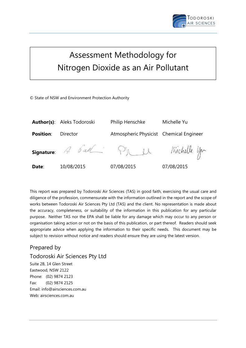
The majority of the NOX emissions in the GMR are dominated by emissions from coal-fired power
stations. In the Sydney region, the industrial NOX emissions arise predominantly from various industrial
sources with a greater proportion from gas-fired power stations followed by petroleum products and
fuel production. Ammonium production is the biggest source of NOX emissions from industries in the
Newcastle region, and in the Wollongong region the majority of NOX emissions arise from iron or steel
production.
Figure 4-3: Proportions of NOX emissions from industrial sources in each region of the GMR in 2008 (NSW EPA, 2012c)

5
Figure 4-4: Proportion of NOX emissions by industrial activity type in the GMR in 2008 (NSW EPA, 2012c)
Figure 4-5: Proportion of NOX emissions by industrial activity type in the Sydney region in 2008 (NSW EPA, 2012c)

6
Figure 4-6: Proportion of NOX emissions by industrial activity type in the Newcastle region in 2008 (NSW EPA, 2012c)
Figure 4-7: Proportion of NOX emissions by industrial activity type in the Wollongong region in 2008 (NSW EPA, 2012c)
7
Figure 4-8: Proportion of NOX emissions by industrial activity type in the non-urban region in 2008 (NSW EPA, 2012c)
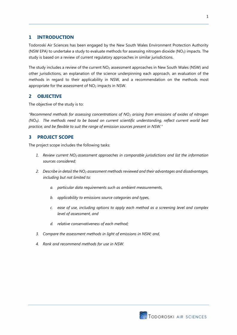
4.1.2 NOx from on-road mobile sources
Emissions from on-road mobile sources are the main source of NOX emissions in the Sydney region, see
Figure 4-2.
As shown in Figure 4-9 the majority of the NOX from on-road mobile sources in the GMR in 2008 arise
in Sydney. Figure 4-10 shows the breakdown of the various on-road mobile NOx sources in the GMR
in 2008, which is dominated by petrol passenger vehicles and heavy-duty diesel vehicles.
The distribution of NOX emissions from each on-road mobile source for each region in the GMR is
presented in Figure 4-11 and shows a similar distribution that is typically dominated by petrol
passenger vehicles and heavy-duty diesel vehicles.

8
Figure 4-9: Proportions of NOx emissions from on-road mobile sources in each region of the GMR in 2008 (NSW EPA, 2012b)
Figure 4-10: Proportion of NOx emissions by on-road mobile source type in the GMR in 2008 (NSW EPA, 2012b)
9
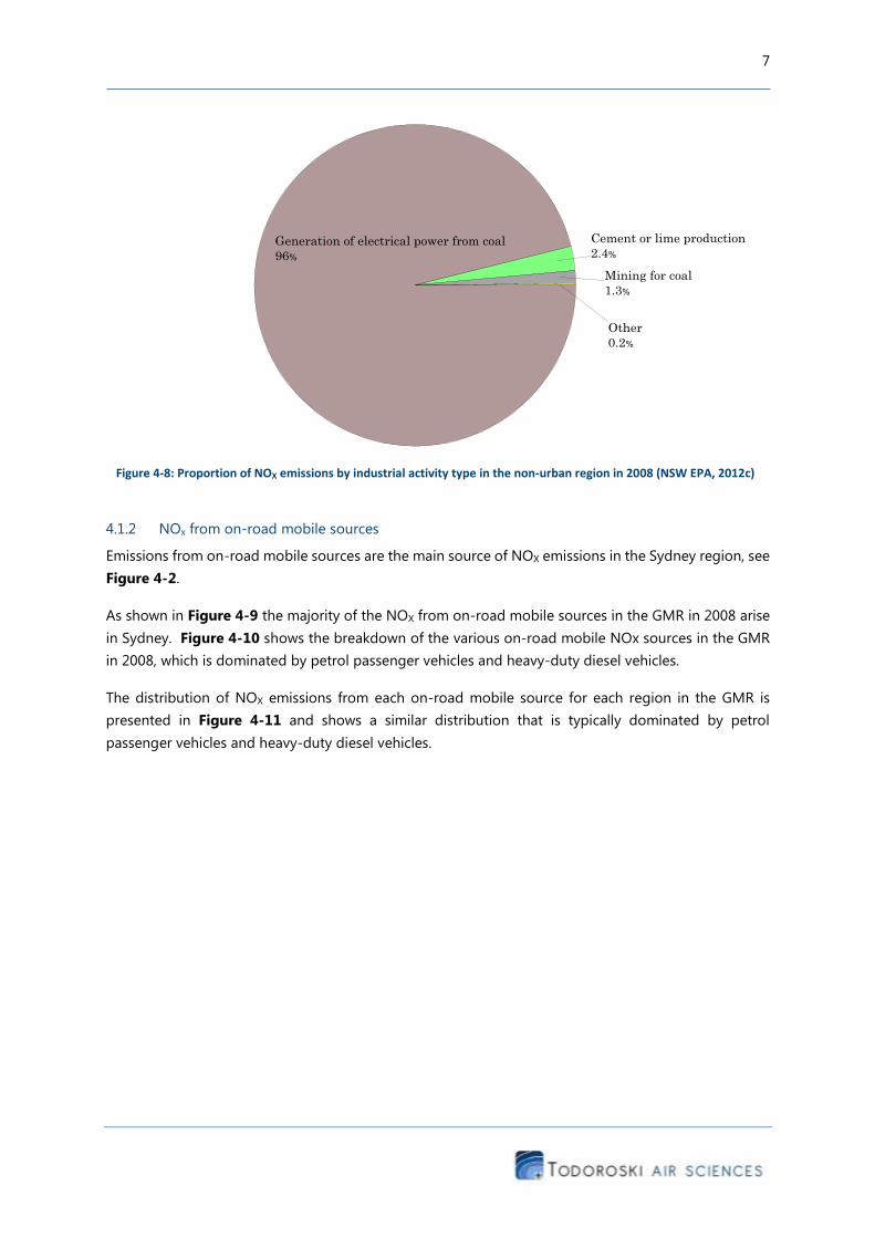
Figure 4-11: Proportion of NOx emissions by on-road mobile source type in Sydney, Newcastle, Wollongong, and Non-Urban
Regions (clockwise from upper left) in 2008 (NSW EPA, 2012b)
Observations of NO and NO2 in Sydney’s M5 East Tunnel suggest that the NO2/NOX ratio from motor
vehicles is approximately 5-6 per cent (NHMRC, 2008). During the daytime the ratio was typically 5 per
cent, while at night time higher ratios were observed due to both lower emissions and the lower
likelihood of oxidant depletion (Holmes Air Sciences as cited in NHMRC, 2008).
10
In London, although there has been a downward trend of NOX concentrations at the roadside from 1997
to 2003, the NO2 concentrations had no significant statistical trend over the same period (Carslaw, 2005).
The relatively flat NO2 concentrations contrasts with a downward trend in NOX concentrations in London
and is believed to be due to the increase of NO2/NOx emissions ratio from motor vehicles from
approximately 5-6% in 1997 to approximately 17% in 2003, on the basis of “hourly modelling using a
simple constrained chemical model” (Carslaw, 2005).
The increase in the NO2/NOx emissions ratio may be due to the increased use of catalytic diesel
particulate filters using an oxidation catalyst, increased use of diesel cars and new engine technologies,
and management approaches (Carslaw, 2005). The introduction of the more stringent Euro 6 emissions
standards in Europe in 2014 would further decrease NOX emissions at the roadside but would increase
the NO2/NOX emissions ratio (Weiss et al., 2012).
These variations in on-road mobile NOx over time highlight that it is important for NO2 assessments to
reflect the current and likely future trend of NO2 and NOX emissions from major sources such as vehicles
which can potentially be inferred from historic trends and the available information on influencing
factors such as the increasing uptake of new or future engine technologies.
4.2 NO2 atmospheric reactions
The atmospheric reaction of NO2 mainly involves the following reactions:
𝑂3 + 𝑁𝑂 → 𝑁𝑂2 + 𝑂2 Reaction 1
𝑁𝑂2 + ℎ𝑣 → 𝑁𝑂 + 𝑂 Reaction 2
The oxidation of NO with O3 (as illustrated in Reaction 1) is a fast reaction (typically a few minutes) in
typical urban atmospheric conditions (ETC/ACM, 2011). In the presence of sunlight, the production of
NO2 is balanced by its photodissociation into NO and ground state oxygen molecule (O), as illustrated
in Reaction 2 where hv is the energy from a photon with a wavelength of less than 420nm (ETC/ACM,
2011).
As demonstrated by these two reactions, the concentration of NO2 is dependent on the O3 levels and
the presence of sunlight. NO2 concentrations are generally highest during winter as lower temperatures
and lesser sunlight in cooler months results in less photochemical destruction of NO2 into O3 (NSW
DECCW, 2010a), and also due to poorer dispersion of emissions.
Some of the ground state oxygen (O) produced in Reaction 2 would react with O2 to form O3 in the
presence of some other molecule (M) as shown in Reaction 3 (ETC/ACM, 2011).
𝑂 + 𝑂2 + 𝑀 → 𝑂3 + 𝑀 Reaction 3
Reactions 1 to 3 show a cyclical interdependence of the concentrations of NO2 and O3 which is
exemplified in the monitoring data for the Sydney region shown in Section 4.3.
The pathways for the oxidation of NO to NO2 include reactions with volatile organic compounds (VOCs).
The peroxy radicals (RO2) generated by the oxidation of the VOCs would oxidise NO to NO2 (ETC/ACM,
2011) as shown in Reaction 4.
11
Therefore the presence of VOCs may increase the NO2 concentrations and, through Reactions 2 and 3,
also increase the O3 concentrations. Reaction 4 is a much slower reaction (typically of an hour or more)
than Reaction 1 (which is typically of a few minutes) (ETC/ACM, 2011).
𝑅𝑂2 + 𝑁𝑂 → 𝑁𝑂2 + 𝑅𝑂 Reaction 4
NO2 in the atmosphere would eventually disappear through the following reaction (ETC/ACM, 2011):
𝑁𝑂2 + 𝑂𝐻 + 𝑀 → 𝐻𝑁𝑂3 + 𝑀 Reaction 5
The reaction of NO2 with hydroxyl radical (OH) in the presence of other molecule (M) (Reaction 5)
typically occurs between a few hours and a number of days (ETC/ACM, 2011).
The concentration of NO2 in the atmosphere is dependent on a number of interrelated reactions
involving oxidants whose production also involves a number of reactions, and the presence of sunlight
and O3, VOC ‘s and their reactive oxides, all of which react with and thus consume NO2.
In other words, the NO2 levels will vary with time and space away from the emissions source(s)
depending on the composition and state of the receiving atmosphere, and it is very difficult to precisely
model this situation. An accurate model that might represent these complex reactions would be unlikely
to be practical to use for routine regulatory assessment purposes, and a simplified model becomes
necessary.
Thus in any practical model that is suitable for routine use for NO2 assessments, it is important that the
model operates with a degree of conservatism (overestimation) in order to reasonably take into account
the inherent inaccuracy that arises due to model simplifications.
4.3 Air quality in Sydney – NO2 and O3
The level of NO2 and O3 in the air shed is a significant factor to consider when conducting an NO2
assessment. For example, as described in Section 4.2, there tends to be an inverse relationship between
NO2 and O3 levels on average or over the longer term.
This section examines the long term, annual and one hour average concentrations of NO2 measured in
the Sydney air shed. This is one of the key NSW air sheds with potential for significant NO2 and
significant O3 levels to occur.
The measured O3 levels are also presented and illustrate the interrelationship between NO2 and O3 levels
as described in Section 4.2. Many of the NO2 assessment methods described in Section 5.3 require
such ambient data inputs to make the necessary calculations.
The 1-hour average and annual average concentration data are presented as these are the averaging
periods applied to assess NO2 levels per the relevant criteria (see Section 5.1).
The long term average NO2 and O3 concentrations at each monitoring station as a fraction of the
maximum concentration are also presented in Figure 4-12. These levels do not correspond to
assessment criteria averaging periods, but do illustrate the underlying trends that may not be apparent
when examining any specific short term period. The long term average concentrations are computed as
the average of the available monitoring data from 1990 to 2014. The fraction is normalised by dividing
12
the long term average concentration for each monitor by the highest of the long term averages among
the monitors. Generally, the monitors which recorded higher NO2 concentrations recorded lower O3
concentrations and vice versa.
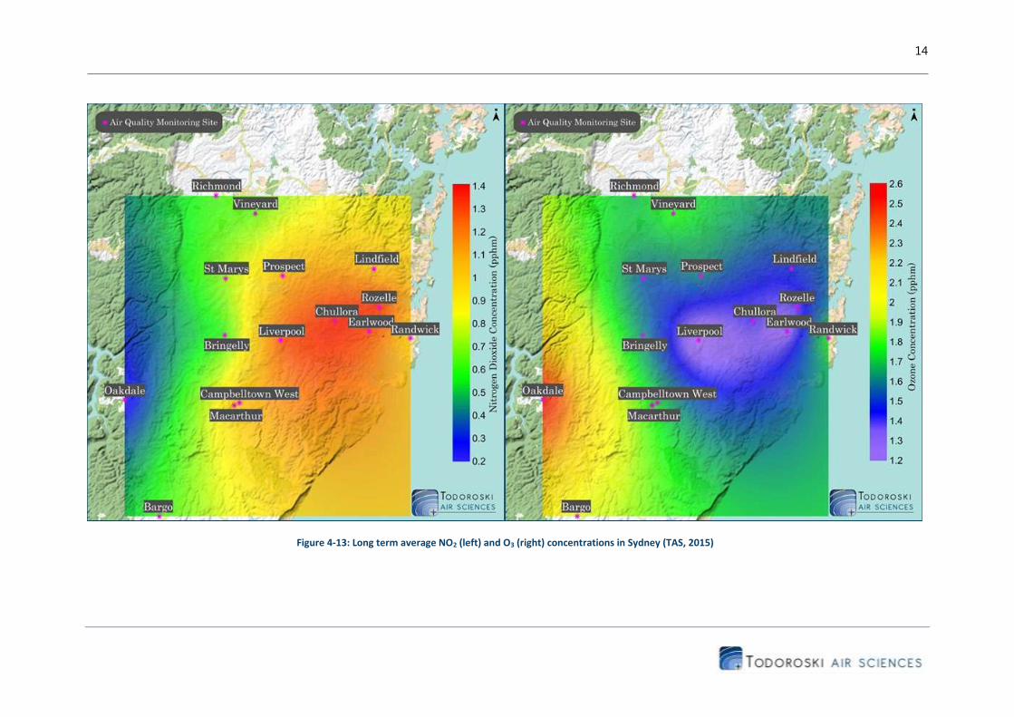
Figure 4-13 presents a spatial distribution plot of the measured long term average NO2 concentration
in the Sydney air shed. The figure indicates that the NO2 concentrations (left) are highest close to the
centre of traffic and industrial activity, but decline to the west where there is a lower density of on-road
mobile sources. The spatial distribution of O3 concentrations (right) shows an opposite trend to the
NO2 concentrations, where the lowest concentrations are found close to the centre of traffic and
industrial activity and increase to the west.
This figure illustrates that over the long term, an inverse relationship between NO2 and O3 does arise in
the Sydney basin, which provides a degree of confidence that assessment methodologies utilising both
NO2 and O3 levels would be applicable in this air shed.
This analysis indicates that in areas with high NOX concentrations, O3 concentrations are typically
depleted through the oxidation of NO to NO2. Further examination of the available ambient NO or NOX
data would be useful to verify this and to examine any related trends in more detail. This is outside the
scope for this project. Nevertheless, the trends in the freely available data indicate that it is likely that
the ambient NO/NO2 ratio would be higher in areas with high O3 levels as more of the NO2 would have
transformed to NO and O3.
It is recommended that it would be useful to extend the study in this regard, and to also examine the
trend each year, to see how changes in industrial and residential development in the air shed may have
spatially influenced the NO/NO2 ratio and O3 levels over time. This may also be a useful analysis to
complete in other urban NSW air sheds with suitable data.

13
Figure 4-12: NO2 and O3 long term averages as a fraction of the maximum concentrations in Sydney (TAS, 2015)
14
Figure 4-13: Long term average NO2 (left) and O3 (right) concentrations in Sydney (TAS, 2015)
15
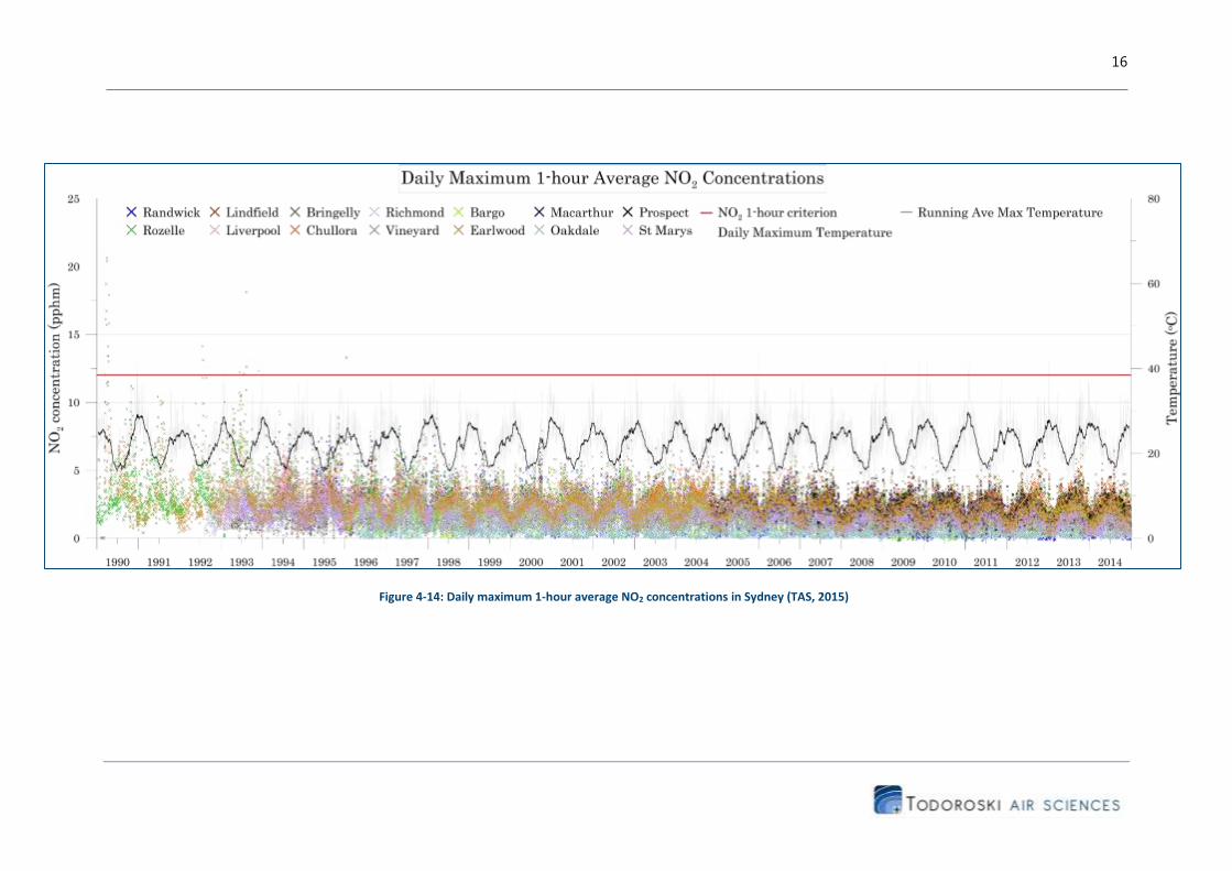
Figure 4-14 and Figure 4-15 present the measured daily maximum 1-hour average NO2 and O3
concentrations, respectively, in Sydney from 1990 to 2014. A seasonal variation in the daily maximum
1-hour concentrations of both species is apparent with NO2 concentrations highest during winter and
lowest during summer, with the opposite trend for O3 concentrations.
During summer, there is more daylight for the photochemical production of O3 and photolysis of NO2
resulting in lower NO2 levels and higher O3 levels.
The 1-hour average NO2 concentrations in the Sydney airshed are well below the criteria and the highest
levels are approximately half of the criteria in recent years. The O3 levels however exceed the criteria in
some hours.
Figure 4-16 and Figure 4-17 present the trend of the annual average NO2 and O3 concentrations,
respectively, in Sydney from 1993 to 2014. The annual average NO2 concentration declines over time,
and levels off from approximately 2009 onwards while the annual average O3 concentration increases
over time and levels off from approximately 2004 onwards. In recent years the levels of NO2 are well
below the relevant criteria with the highest levels reaching approximately half of the criteria.
16
Figure 4-14: Daily maximum 1-hour average NO2 concentrations in Sydney (TAS, 2015)

17
Figure 4-15: Daily maximum 1-hour average O3 concentrations in Sydney (TAS, 2015)

18
Figure 4-16: Annual average NO2 concentrations in Sydney (TAS, 2015)

19
Figure 4-17: Annual average O3 concentrations in Sydney (TAS, 2015)
20
5 REVIEW OF NO2 IMPACT ASSESSMENT REQUIREMENTS
As outlined previously, NO2 concentrations from anthropogenic sources arise from direct emissions and
NO2 that is produced from the atmospheric oxidation of NO. The chemistry involved in the atmospheric
reaction is complex and involves many variables such as the presence of UV to catalyse the
photochemical reactions involving NOX, VOCs and O3, and the inhomogeneous mixing of the reactants
in the open atmosphere.
This complex chemistry in the production and depletion of NO2 occurs while the reactants are dispersing
in the atmosphere. Since the various mechanisms and variables involved in the production of NO2 are
difficult to simulate, simple approaches for predicting NO2 impacts have been developed using easily
obtainable information such as ambient O3 concentrations. Such approaches may rely on formulae or
variables specific to the various jurisdictions in which they are used to assess potential NO2 impacts per
the various criteria applicable in these jurisdictions. These factors need to be considered when
determining the applicability of these approaches to NSW, along with the ability of the methods to
produce results that can be assessed against the relevant NSW 1-hour and annual average periods for
assessment (see Section 5.1).
5.1 Current approaches in NSW
To demonstrate compliance with relevant criteria, a Level 1 or Level 2 assessment may be employed as
set out in the Approved Methods for the Modelling and Assessment of Air Pollutants in New South Wales
(NSW DEC, 2005). Table 5-1 summarises the air quality goals for the assessment of NO2 in NSW.
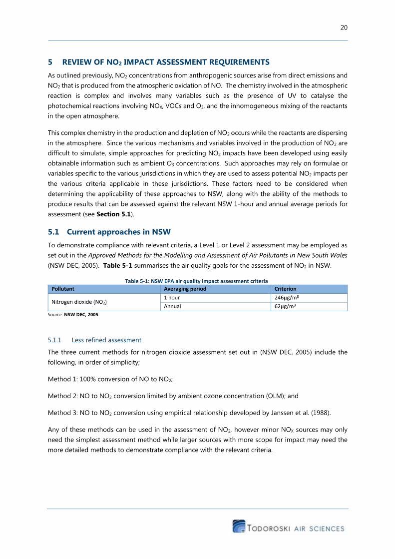
Table 5-1: NSW EPA air quality impact assessment criteria
Pollutant Averaging period Criterion
Nitrogen dioxide (NO2) 1 hour 246µg/m3
Annual 62µg/m3
Source: NSW DEC, 2005
5.1.1 Less refined assessment
The three current methods for nitrogen dioxide assessment set out in (NSW DEC, 2005) include the
following, in order of simplicity;
Method 1: 100% conversion of NO to NO2;
Method 2: NO to NO2 conversion limited by ambient ozone concentration (OLM); and
Method 3: NO to NO2 conversion using empirical relationship developed by Janssen et al. (1988).
Any of these methods can be used in the assessment of NO2, however minor NOX sources may only
need the simplest assessment method while larger sources with more scope for impact may need the
more detailed methods to demonstrate compliance with the relevant criteria.
21
5.1.2 Detailed assessment of NO2
More detailed models for NO2 assessment are outlined in (NSW DEC, 2005), and include the following
methods developed by CSIRO.
Integrated Empirical Rate (IER) Reactive Plume Model. The IER Reactive Plume Model is a more refined
assessment method than the methods specified above. It not only predicts changes in ambient NO2
concentrations but also ambient O3 concentrations (NSW DEC, 2005).
The Air Pollution Model (TAPM). “CSIRO TAPM includes gas-phase photochemistry based on the semi-
empirical mechanism, called the Generic Reaction Set (GRS). In chemistry mode, TAPM includes 10
reactions for the following 13 species: smog reactivity, radical pool, hydrogen peroxide (H2O2), NO, NO2,
O3, SO2, stable non-gaseous organic carbon, stable gaseous nitrogen products, stable non-gaseous
nitrogen products, stable non-gaseous sulfur products, airborne particulate matter and fine particulate
matter” (NSW DEC, 2005).
Generally, the less refined methods are sufficient for most NO2 impact assessment requirements.
5.2 Approaches in various other jurisdictions
Table 5-2 presents a summary of the NO2 impact criteria and assessment approaches in various
jurisdictions identified through a desktop literature review.
The scientific basis underpinning each of the methods presented in the table is briefly described in
Section 5.3.

22
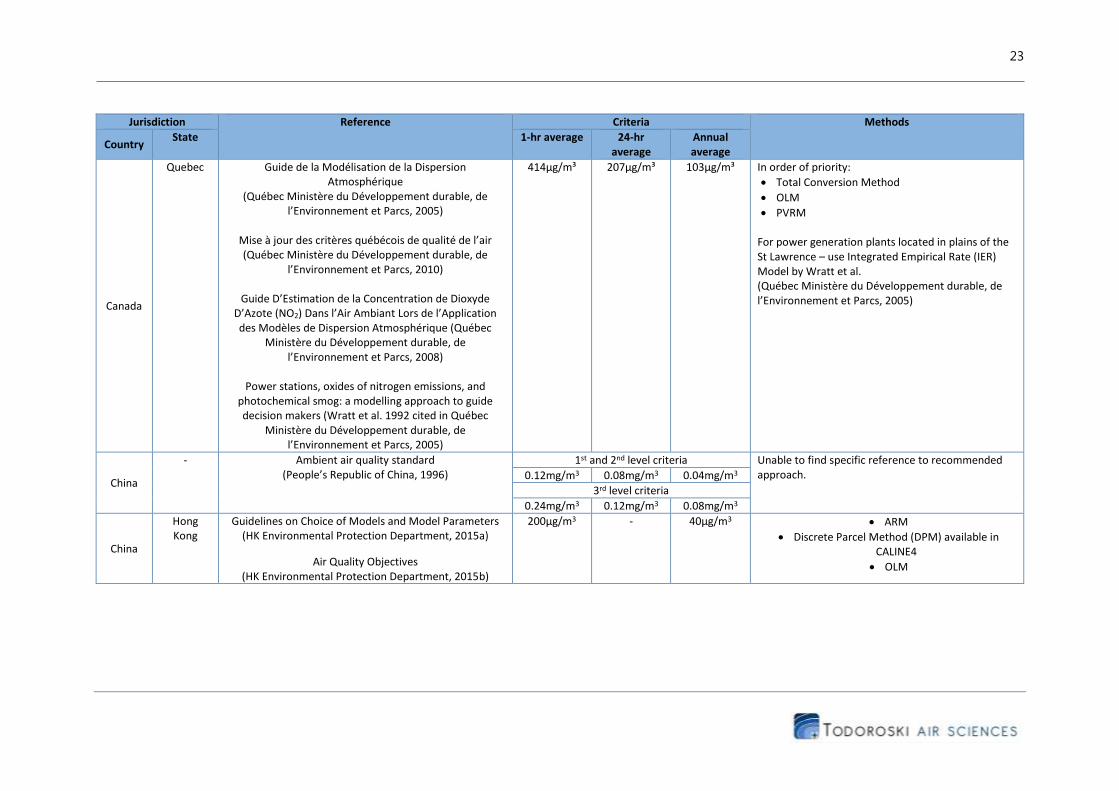
Table 5-2: Summary of the current NO2 impact criteria and assessment approaches in various jurisdictions
Jurisdiction Reference Criteria Methods
Country State 1-hr average 24-hr
average Annual average
Canada
Alberta Air Quality Modelling Guideline (Alberta Environment, 2009)
Draft Proposed Air Quality Modelling Guideline (Alberta ESRD, 2012)
Alberta Ambient Air Quality Objectives and Guidelines Summary (Alberta Environment, 2013)
300µg/m3 (159ppb)
- 45µg/m3 (24ppb)
Total Conversion Method
Plume Volume Molar Ratio Method (PVMRM) in AERMOD
RIVAD/ARM3 Chemical Formulations in CALPUFF
Ozone Limiting Method (OLM)
Ambient Ratio Method (ARM)
Canada
British Columbia
Guidelines for Air Quality Dispersion Modelling in British Columbia (BC Ministry of Environment, 2008)
British Columbia Ambient Air Quality Objectives
(BC Ministry of Environment, 2014)
188µg/m3 (100ppb)
- 60µg/m3 (32ppb)
In order of priority:
Total Conversion Method
ARM
OLM
PVRM in AERMOD
Canada
Ontario Air Dispersion Modelling Guideline for Ontario (Ontario Ministry of the Environment, 2009)
Ontario’s Ambient Air Quality Criteria (Ontario Ministry of the Environment, 2012)
400µg/m3 (0.20ppm)
200µg/m3 (0.10ppm)
- Not specifically mentioned but refers to OLM and PVMRM as AERMOD options. Refers to post processing approaches described in the US EPA Guidelines on Air Quality Models.
Canada
Manitoba Manitoba Ambient Air Quality Criteria (Manitoba Government, 2005)
Maximum Tolerable Level Concentration Not specifically stated however indicates reference to US EPA Guidelines. 1000µg/m3
(0.53ppm) - -
Maximum Acceptable Level Concentration
400µg/m3 (0.213ppm)
200µg/m3 (0.106ppm)
100µg/m3 (0.053ppm)
Maximum Desirable Level Concentration
- - 60µg/m3 (0.032ppm)
Canada
Newfoundland
Labrador
Guideline for Plume Dispersion Modelling (Newfoundland and Labrador DEC, 2012)
Air Pollution Control Regulations (2004)
400µg/m3 200µg/m3 100µg/m3 RIVAD/ISORROPIA for CALPUFF assessments
PVMRM for AERMOD and AERSCREEN applications
Canada
Saskatchewan
Saskatchewan Air Quality Modelling Guideline (Saskatchewan Ministry of Environment, 2012)
Ambient Air Quality Standards (The Clean Air Act, 2014)
400µg/m3 (0.2ppm)
- 100µg/m3 (0.05ppm)
Total Conversion Method
ARM
OLM
PVMRM
23
Jurisdiction Reference Criteria Methods
Country State 1-hr average 24-hr
average Annual average
Canada
Quebec Guide de la Modélisation de la Dispersion Atmosphérique
(Québec Ministère du Développement durable, de l’Environnement et Parcs, 2005)
Mise à jour des critères québécois de qualité de l’air (Québec Ministère du Développement durable, de
l’Environnement et Parcs, 2010)
Guide D’Estimation de la Concentration de Dioxyde D’Azote (NO2) Dans l’Air Ambiant Lors de l’Application des Modèles de Dispersion Atmosphérique (Québec
Ministère du Développement durable, de l’Environnement et Parcs, 2008)
Power stations, oxides of nitrogen emissions, and
photochemical smog: a modelling approach to guide decision makers (Wratt et al. 1992 cited in Québec
Ministère du Développement durable, de l’Environnement et Parcs, 2005)
414µg/m³ 207µg/m³ 103µg/m³ In order of priority:
Total Conversion Method
OLM
PVRM
For power generation plants located in plains of the St Lawrence – use Integrated Empirical Rate (IER) Model by Wratt et al. (Québec Ministère du Développement durable, de l’Environnement et Parcs, 2005)
China
- Ambient air quality standard (People’s Republic of China, 1996)
1st and 2nd level criteria Unable to find specific reference to recommended approach. 0.12mg/m3 0.08mg/m3 0.04mg/m3
3rd level criteria
0.24mg/m3 0.12mg/m3 0.08mg/m3
China
Hong Kong
Guidelines on Choice of Models and Model Parameters (HK Environmental Protection Department, 2015a)
Air Quality Objectives (HK Environmental Protection Department, 2015b)
200µg/m3 - 40µg/m3 ARM
Discrete Parcel Method (DPM) available in CALINE4
OLM
24
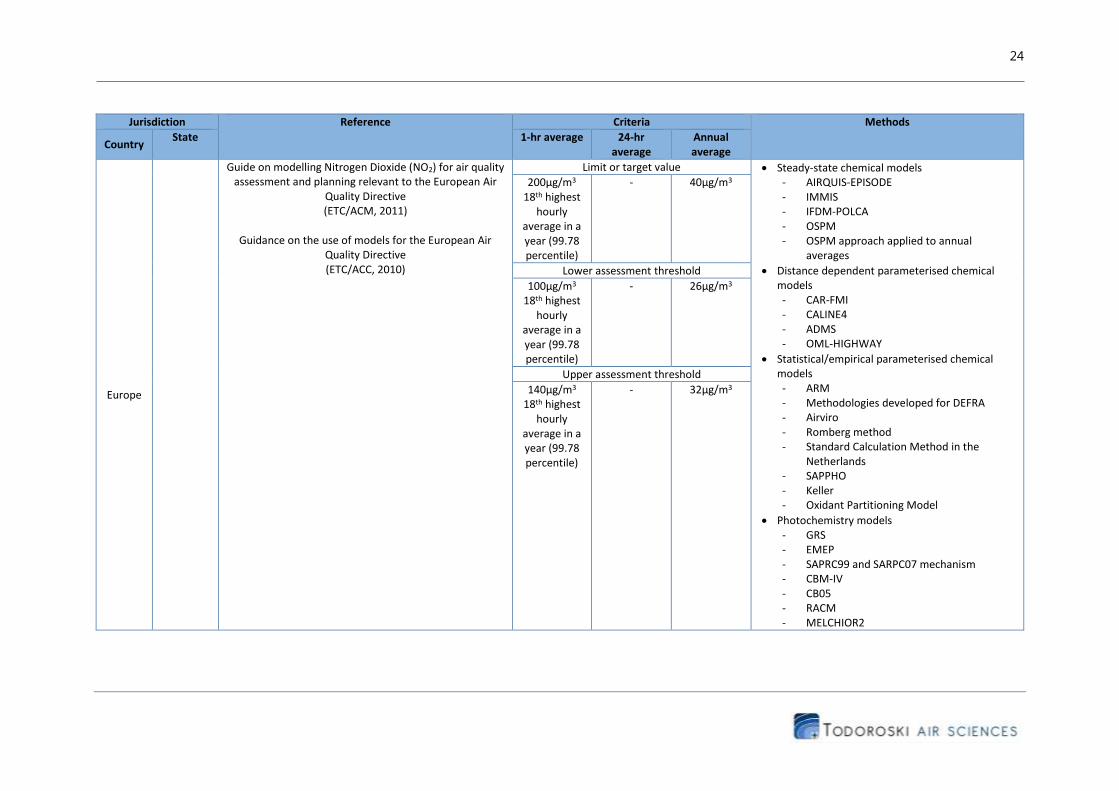
Jurisdiction Reference Criteria Methods
Country State 1-hr average 24-hr
average Annual average
Europe
Guide on modelling Nitrogen Dioxide (NO2) for air quality assessment and planning relevant to the European Air
Quality Directive (ETC/ACM, 2011)
Guidance on the use of models for the European Air
Quality Directive (ETC/ACC, 2010)
Limit or target value Steady-state chemical models - AIRQUIS-EPISODE - IMMIS - IFDM-POLCA - OSPM - OSPM approach applied to annual
averages
Distance dependent parameterised chemical models - CAR-FMI - CALINE4 - ADMS - OML-HIGHWAY
Statistical/empirical parameterised chemical models - ARM - Methodologies developed for DEFRA - Airviro - Romberg method - Standard Calculation Method in the
Netherlands - SAPPHO - Keller - Oxidant Partitioning Model
Photochemistry models - GRS - EMEP - SAPRC99 and SARPC07 mechanism - CBM-IV - CB05 - RACM - MELCHIOR2
200µg/m3 18th highest
hourly average in a year (99.78 percentile)
- 40µg/m3
Lower assessment threshold
100µg/m3 18th highest
hourly average in a year (99.78 percentile)
- 26µg/m3
Upper assessment threshold
140µg/m3 18th highest
hourly average in a year (99.78 percentile)
- 32µg/m3
25
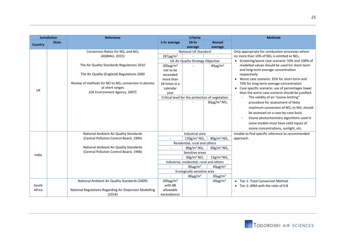
Jurisdiction Reference Criteria Methods
Country State 1-hr average 24-hr
average Annual average
UK
Conversion Ratios for NOx and NO2 (AQMAU, 2015)
The Air Quality Standards Regulations 2010
The Air Quality (England) Regulations 2000
Review of methods for NO to NO2 conversion in plumes
at short ranges (UK Environment Agency, 2007)
National UK Standard Only appropriate for combustion processes where no more than 10% of NOx is emitted as NO2.
Screening/worst case scenario: 50% and 100% of modelled values should be used for short-term and long-term average concentration respectively
Worst case scenario: 35% for short-term and 70% for long-term average concentration
Case specific scenario: use of percentages lower than the worst case scenario should be justified. - The validity of an “ozone-limiting”
procedure for assessment of likely
maximum conversion of NOx to NO2 should
be assessed on a case-by-case basis
- Ozone photochemistry algorithms used in
some models must have valid inputs of
ozone concentrations, sunlight, etc.
287µg/m3 - -
UK Air Quality Strategy Objective
200µg/m3 not to be exceeded more than
18 times in a calendar
year
- 40µg/m3
Critical level for the protection of vegetation
- - 30µg/m3 NOx
India
National Ambient Air Quality Standards (Central Pollution Control Board, 1994)
National Ambient Air Quality Standards (Central Pollution Control Board, 1998)
Industrial area Unable to find specific reference to recommended approach. - 120g/m3 NOx 80g/m3 NOx
Residential, rural and others
- 80g/m3 NOx 60g/m3 NOx
Sensitive areas
30g/m3 NOx 15g/m3 NOx
Industrial, residential, rural and others
- 80µg/m3 40µg/m3
Ecologically sensitive area
- 80µg/m3 30µg/m3
South Africa
National Ambient Air Quality Standards (2009)
National Regulations Regarding Air Dispersion Modelling (2014)
200µg/m3 with 88
allowable exceedances
40µg/m3 Tier 1: Total Conversion Method
Tier 2: ARM with the ratio of 0.8

26
Jurisdiction Reference Criteria Methods
Country State 1-hr average 24-hr
average Annual average
Japan
Air Pollution Control Technology Manual (Overseas Environmental Cooperation Center, 1998)
- Within the 0.04-
0.06ppm zone or below.
- Exponential function model 𝑁𝑂2
𝑁𝑂𝑋= 1 −
𝑎
1 + 𝑏 (exp(−𝑘𝑡) + 𝑏)
k = 0.0062UO3B (stationary sources, vessels) or k = 0.208UO3B (automobiles, houses) b = 0.3 a = 0.9 Here, t is time, U is velocity and O3B is concentration of Ozone. Statistical model
𝑁𝑂2 = 𝑎[𝑁𝑂𝑋]𝑏 Where a and b are determined using observed data. The exponential function is generally used in estimating NO2 impacts from stationary sources and the statistical model is used for automobile influences.
Australia
QLD Environmental Protection (Air) Policy 2008 Health and wellbeing Indicates reference to NSW EPA Guidelines.
250µg/m3 with
allowable exceedance of 1 day per
year
- 62µg/m3
Health and biodiversity of ecosystems
- - 33µg/m3
Australia
SA EPA Guidelines - Air quality impact assessment using design ground level pollutant concentrations (DGLCs)
(SA EPA, 2006)
In Adelaide metro areas Unable to find specific reference to recommended approach. 0.113mg/m3 - -
Outside Adelaide metro areas
0.158mg/m3 - -
27
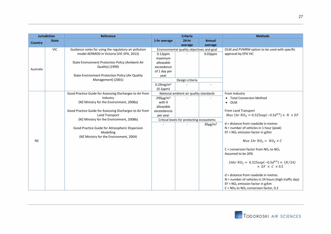
Jurisdiction Reference Criteria Methods
Country State 1-hr average 24-hr
average Annual average
Australia
VIC Guidance notes for using the regulatory air pollution model AERMOD in Victoria (VIC EPA, 2013)
State Environment Protection Policy (Ambient Air
Quality) (1999)
State Environment Protection Policy (Air Quality Management) (2001)
Environmental quality objectives and goal OLM and PVMRM option to be used with specific approval by EPA VIC 0.12ppm
maximum allowable
exceedance of 1 day per
year
- 0.03ppm
Design criteria
0.29mg/m3 (0.1ppm)
- -
NZ
Good Practice Guide for Assessing Discharges to Air from Industry
(NZ Ministry for the Environment, 2008a)
Good Practice Guide for Assessing Discharges to Air from Land Transport
(NZ Ministry for the Environment, 2008b)
Good Practice Guide for Atmospheric Dispersion Modelling
(NZ Ministry for the Environment, 2004)
National ambient air quality standards From Industry
Total Conversion Method
OLM
From Land Transport
𝑀𝑎𝑥 1ℎ𝑟 𝑁𝑂𝑋 = 0.325exp(−0.3𝑑0.5) × 𝑁 × 𝐸𝐹
d = distance from roadside in metres N = number of vehicles in 1 hour (peak) EF = NOx emission factor in g/km
𝑀𝑎𝑥 1ℎ𝑟 𝑁𝑂2 = 𝑁𝑂𝑋 × 𝐶
C = conversion factor from NOx to NO2 Assumed to be 20%
24ℎ𝑟 𝑁𝑂2 = 0.325exp(−0.3𝑑0.5) × (𝑁 24⁄ )
× 𝐸𝐹 × 𝐶 × 0.5
d = distance from roadside in metres N = number of vehicles in 24 hours (high traffic day) EF = NOx emission factor in g/km C = NOX to NO2 conversion factor, 0.2
200µg/m3 with 9
allowable exceedances
per year
- -
Critical levels for protecting ecosystems
- - 30µg/m3
28
Jurisdiction Reference Criteria Methods
Country State 1-hr average 24-hr
average Annual average
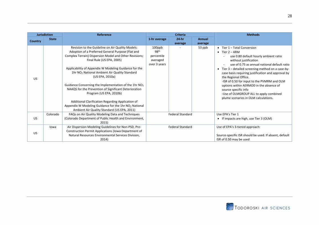
US
Revision to the Guideline on Air Quality Models: Adoption of a Preferred General Purpose (Flat and
Complex Terrain) Dispersion Model and Other Revisions; Final Rule (US EPA, 2005)
Applicability of Appendix W Modeling Guidance for the
1hr NO2 National Ambient Air Quality Standard (US EPA, 2010a)
Guidance Concerning the Implementation of the 1hr NO2
NAAQS for the Prevention of Significant Deterioration Program (US EPA, 2010b)
Additional Clarification Regarding Application of
Appendix W Modeling Guidance for the 1hr NO2 National Ambient Air Quality Standard (US EPA, 2011)
100ppb 98th
percentile averaged
over 3 years
- 53 ppb Tier 1 – Total Conversion
Tier 2 – ARM - use 0.80 default hourly ambient ratio
without justification - use of 0.75 as annual national default ratio
Tier 3 – detailed screening method on a case-by-case basis requiring justification and approval by the Regional Office. -ISR of 0.50 for input to the PVMRM and OLM options within AERMOD in the absence of source specific info -Use of OLMGROUP ALL to apply combined plume scenarios in OLM calculations.
US Colorado FAQs on Air Quality Modeling Data and Techniques
(Colorado Department of Public Health and Environment, 2015)
Federal Standard Use EPA’s Tier 1
If impacts are high, use Tier 3 (OLM)
US
Iowa Air Dispersion Modeling Guidelines for Non-PSD, Pre-Construction Permit Applications (Iowa Department of
Natural Resources Environmental Services Division, 2014)
Federal Standard Use of EPA’s 3-tiered approach: Source-specific ISR should be used. If absent, default ISR of 0.50 may be used

29
Jurisdiction Reference Criteria Methods
Country State 1-hr average 24-hr
average Annual average
US
California Modeling Compliance of The Federal 1-Hour NO2 NAAQS (CAPCOA, 2011)
Nitrogen Dioxide – Overview (CARB, 2011)
California Standard Use US EPA guidance (3-tiered approach)
1. Significant Impact Level (SIL) 2. Max Modeled + Max Monitor Value 3. Max Modeled + 98th Monitor value 4. 8th Highest Modeled + Max Monitor Value 5. 8th Highest Modeled + 98th Monitor Value 6. 5yr ave of the 98th percentile + Max
Monitor Value 7. 5yr ave of the 98th percentile + 98th
monitor value 8. 5yr ave of the 98th percentile + monthly
hour-of-day (1st highest) 9. 5yr ave of the 98th percentile + Seasonal
hour-of-day (3rd highest) 10. 5yr ave of the 98th percentile + Annual
Hour-of-Day (8th Highest) 11. Paired-Sum (5yr Ave of the 98th percentile)
0.18ppm - 0.030ppm
Federal Standard
US
New York NYSDEC Guidelines on Dispersion Modeling Procedures for Air Quality Impact Analysis (NYS DEC, 2006)
Federal Standard Screening methods 1. Gaussian model with total conversion of NOx to NO2 2.ARM using default of 0.75 ratio or site-specific ratio Refined method - Case-by-case analysis
US
Ohio Engineering Guide #69: Air Dispersion Modeling Guidance (Ohio EPA, 2014)
Federal Standards Refers to US EPA’s guidelines
Ohio EPA Generally Acceptable Incremental Impact
188µg/m3 - 12.5µg/m3
US Rhode Island
Rhode Island Air Dispersion Modeling Guidelines for Stationary Sources (Rhode Island Department of
Environmental Management, 2013)
Federal Standards US EPA approach
US Texas Air Quality Modeling Guidelines (Texas Commission on
Environmental Quality, 2014) Federal Standards US EPA Approach
30
5.3 Description of methods for NO2 assessment
5.3.1 Total Conversion Method
The Total Conversion Method assumes 100 per cent conversion of NO to NO2. This is the simplest and
most conservative method of evaluating NO2 impacts from NOX sources. Due to the conservative nature
of the method, no justification is needed for its use and it is often applied as the screening method for
the assessment of NO2 impacts (Level 1 assessment) in various jurisdictions.
5.3.2 Ambient Ratio Method
The Ambient Ratio Method (ARM) uses an NO2 to NOx ratio to predict the NO2 impact from the NOX
concentrations. The principle behind the ARM is that a source plume NO2 to NOx ratio will be the same
in the long-term as the existing ambient NO2 to NOx ratio (OLM/ARM Workgroup, 1998). To determine
the NO2 to NOx ratio, ambient NO2 and NOx data from monitoring stations located away from the source
(approximately 15 to 60km downwind) (Hanrahan, 1999a) are needed.
Ambient NOX monitoring however is not always sufficient to determine the ratio as the ambient
concentrations are often below the minimum concentration threshold for NOX of 20ppb (Hanrahan,
1999a). This is a potential limitation in NSW where hourly NOX monitoring data would not appear to
be publically available (i.e. it may be necessary to report this data if ARM is to be adopted). Further, NO2
to NOX ratios should only be determined using NOX concentration data of at least 20ppb (OLM/ARM
Workgroup, 1998 from Chu & Meyer, 1991). The inclusion of NOx concentration data that are less than
20ppb would introduce “potentially large errors introduced by small signal to noise ratios typical of
current monitoring instrument at low ambient levels of NOx” (OLM/ARM Workgroup, 1998 from Chu &
Meyer, 1991). This situation may have improved with advancements in monitoring equipment.
As the source plume will only achieve the ambient ratio on a long-term basis, the method has been
originally used only for the estimation of the annual average NO2 concentrations (US EPA, 2005). Chu
and Meyer recommended using the daily average concentration during daylight hours to determine the
annual average NO2 and NOX concentrations (OLM/ARM Workgroup, 1998). Night-time data should
not be used to eliminate the low NO2 bias to get a conservative NO2 to NOX ratio (OLM/ARM
Workgroup, 1998 from Chu & Meyer, 1991).
The OLM/ARM Workgroup (1998) recommends using the annual average concentrations rather than
the average daily average approach by Chu and Meyer as the ARM theory will only be true if the
predicted and the observed NO2 and NOX concentrations are averaged in the same way.
The US EPA (2011) has recommended a fixed ratio of 0.8 for modelling hourly NO2 concentrations when
applying the ARM, based on ambient NO2/NOX ratios from studies by Wang et al (2011) and Jansenn
et al (1991).
5.3.3 Ambient Ratio Method 2
The Ambient Ratio Method 2 (ARM2) is a modified version of the ARM. ARM2 is based on observed
hourly NO2/NOX concentration ratios from a large data set with diverse source-monitor distances,
atmospheric ozone concentrations, and atmospheric dispersion conditions (Podrez, 2015). The upper
limits of the observed NO2 to NOx ratio with the observed NOx concentration are used to derive the

31
empirical relationship and are found to perform better than ARM and produce comparable results for
more refined 1-hour NO2 modelling (RTP Environmental Associates, 2013).
Studies show that the NO2 to NOX ratio increases with distance from the source, and thus using the
ARM method would tend to overestimate the NO2 predictions near the source (RTP Environmental
Associates, 2013).
A variable NO2 to NOX ratio with distance would predict a more realistic NO2 concentration. By plotting
the NO2 to NOX ratio as a function of the NOX concentration, it was found to produce a similar
relationship to plotting the ratio as a function of the inverse distance (Podrez, 2012).
Thus, the variable ratio has been developed for determining the NO2 to NOX ratio as a function of NOX
concentrations. This method removes challenges associated with distance to monitoring stations and
the influence of other sources. The ARM2 approach has been incorporated into AERMOD version 14134
(Podrez, 2015).
5.3.4 Ozone Limiting Method
The Ozone Limiting Method (OLM) predicts the NO2 concentration with the assumption that NO and
O3 react to form NO2 in proportion to their receptor concentrations (Hanrahan, 1999a). It assumes total
conversion of either NO or O3, whichever is limiting, based on the receptor NO and O3 concentrations.
It requires an in-stack NO2 concentration contribution to be added to the NO2 concentration formed by
reaction with ozone.
OLM neglects the oxidation of NO to NO2 by oxidants other than ozone and ignores the
photodissociation of NO2 (Cole & Summerhays, 1979). “The actual reactions occur in proportion to the
moles of each reactant rather than in proportion to concentration” which would make OLM theoretically
valid if the reaction occurs in a closed system (Hanrahan, 1999a). However, as the atmosphere is an
open system, there is practically an unlimited amount of O3 available for reaction and some of the NO
would have been converted to NO2 as the plume travels to the receptor (Hanrahan, 1999a).
The US EPA limits the use of OLM to a single plume at a time unless the plumes overlap (US EPA, 2010).
5.3.5 Plume Volume Molar Ratio Method
The Plume Volume Molar Ratio Method (PVMRM) addresses some of the limitations of the OLM.
PVMRM takes into account the expansion of the plume and the reaction of NO with O3 as the plume
expands downwind by “computing the number of moles of NOX and O3 that are contained within a
plume segment as it reaches a receptor” (Hanrahan, 1999a). In a plume segment, the amount of primary
NOX remains the same as it travels downwind but the amount of O3 increases as the segment expands
downwind (Hanrahan, 1999a).
PVMRM has been found to predict close to the measured values while still being conservative
(Hanrahan, 1999a and 1999b).
5.3.6 RIVAD/ARM3 in CALPUFF
The Acid Rain Mountain Mesoscale Model (ARM3) predicts acid deposition and air quality impacts with
chemical transformation in complex terrain at mesoscale distances (Morris et al, 1989). ARM3 was found
to perform as good as, or even better than, other mesoscale models in terms of transport or dispersion.
32
However its chemical transformation and deposition component has not been evaluated (Moore et al,
1990). RIVAD is one of the chemical transformation schemes available in the ARM3.
The RIVAD is a condensed pseudo-first-order chemical scheme available in CALPUFF as prepared for
the ARM3 (Earth Tech, 2000). The scheme assumes a low VOC background concentration and is thus
not suitable for urban areas (Earth Tech, 2000). The scheme includes solving the pseudo-steady-state
concentrations of NO, NO2 and O3 from the photolysis of NO2 to NO and O3 and the reaction of NO
and O3 to NO2 (Atmospheric and Environmental Research, 2008). In the revised RIVAD/ARM3 scheme
of CALPUFF, the puff O3 concentration is consumed by the oxidation of NO and is replenished by the
background O3 concentration (Atmospheric and Environmental Research, 2008).
Thus, the puff O3 concentration is the average, weighted by the change in the puff volume, of the puff
O3 concentration for the previous time step and the background concentration (Atmospheric and
Environmental Research, 2008). The original RIVAD/ARM3 scheme in CALPUFF does not take into
account the depletion of O3 in the plume and has still been retained as an option in CALPUFF as
MCHEM=3, while the revised RIVAD/ARM3 scheme is a new option as MCHEM=5 (Atmospheric and
Environmental Research, 2008). The difference in the results of the original and revised RIVAD/ARM3
was not significant in the case studies for which they were evaluated (Atmospheric and Environmental
Research, 2008).
5.3.7 Discrete Parcel Method in CALINE4
The Discrete Parcel Method predicts the NO2 impacts by assuming that the oxidation and dissociation
of NOx occurs in isolated discrete parcels of mixed reactants (Benson, 1989). The method assumes that
the reactants are initially fully mixed within the mixing zone, the initial NOX emissions are composed of
92.5 per cent NO and 7.5 per cent NO2 by mass, and that the parcels of reactants are isolated for a
certain time/distance before molecular diffusion takes place (Benson, 1989). Plume travel times are not
long enough for diffusion to significantly take place in the discrete parcels for most of the microscale
modelling applications (Benson, 1989).
As the reactions in the parcels occur independently from their dispersion, the time-averaged NO2
concentrations are computed in CALINE4 by adjusting the initial NO2 emission to be equal to the
discrete parcel NO2 concentration after time t for each element-receptor combination and then
computes the time-averaged NO2 concentration as with non-reactive species (Benson, 1989).
A study by Wang et al (2011) has found that CALINE4 predicts the NOX profiles well but under predicts
NO2 concentrations at high wind speed. Also the initial emission of 5 per cent NO2 by volume (or 7.5
per cent by mass) is not likely to be appropriate for most roadways (Wang et al, 2011). Another study
by Levitin et al (2005) has found that CALINE4 predicts NOX and NO2 well and performs similarly to CAR-
FMI. However the performance of either model deteriorates with decreasing wind speed and as the
wind direction approaches a direction parallel to the road.
5.3.8 Methodologies developed for DEFRA
Empirical methods for calculating the NO2 concentrations from the NOx concentrations for the roadside
have been developed in the UK. Derwent and Middleton (1996) developed an empirical relationship
between hourly NO2 and NOX from monitoring data for a kerbside site in London (UK Environment
Agency, 2007). The Derwent-Middleton curve has been used by a number of local authorities, as part

33
of the Aeolius street canyon model and in the ADMS model (UK Environment Agency, 2007). The
Derwent-Middleton curve follows the equation (UK Environment Agency, 2007):
[𝑁𝑂2] = 2.166 − [𝑁𝑂𝑥](1.236 − 3.348𝐴10 + 1.933𝐴102 − 0.326 𝐴10
3
Where A10 = log10([NOx])
Another study examined the relationship between NO2 and NOX concentrations (Dixon et al as cited in
UK Environment Agency, 2007). The study uses a larger dataset of 12 study sites over 7 consecutive
years of data (UK Environment Agency, 2007). The Dixon-Middleton-Derwent curve follows the
equation (UK Environment Agency, 2007):
𝑌2 = 𝐴 + 𝐵𝐴10 + 𝐶𝐴102 + 𝐷𝐴10
3 + 𝐸𝐴104
Where Y2 = [NO2]/[NOx] and A, B, C, D and E are published constants.
Laxen and Wilson used more stations and years in the dataset and provided a simpler relationship for
the annual average NO2 from NOx measurements which is as follows (ETC/ACM, 2011):
[𝑁𝑂2(𝑟𝑜𝑎𝑑)] = (−0.068 log([𝑁𝑂𝑥(𝑡𝑜𝑡𝑎𝑙)]) + 0.53)[𝑁𝑂𝑥(𝑟𝑜𝑎𝑑)]
Where [NOX(total)] = [NOX(road)] + [NOX(background)]
5.3.9 Airviro
Airviro developed the following relationship to determined NO2 concentrations from NOX
concentrations (ETC/ACM, 2011). The formula is based on the existence of a statistical relation between
the NO2/NOX ratio to the absolute NOX level, in that the ratio normally is higher for low NOX
concentration values.
[𝑁𝑂2] = 0.73[𝑁𝑂𝑥]exp (−0.00452[𝑁𝑂𝑥] + 0.003014[𝑁𝑂𝑥]2
5.3.10 Romberg Method
The Romberg method has been used in Germany within a number of models such as PROKAS, IMMIS
and MISKAM and has the following relationship (ETC/ACM, 2011):
[𝑁𝑂2] = 𝐴[𝑁𝑂𝑥]
[𝑁𝑂𝑥] + 𝐵 + 𝐶[𝑁𝑂𝑥]
Where A, B and C are constants determined from monitoring data.
The parameters of the Romberg method were updated by Bächlin et al. using more recent NO2 and NOX
monitoring data (Düring et al, 2011).
5.3.11 Standard Calculation Method in the Netherlands
An empirical relation for the calculation of NO2 contributions from traffic emissions was developed and
refined in the Netherlands. It is presently used in many Dutch legislated models as part of the “Standard
Calculation Method (SCM)” applied in the Netherlands which is as follows (ETC/ACM, 2011):
∆𝑁𝑂2 = 𝐹 ∙ ∆𝑁𝑂𝑥
+ 𝛽 ∙ 𝑂3𝑎 ∙
(1 − 𝐹) ∙ ∆𝑁𝑂𝑥
(1 − 𝐹) ∙ ∆𝑁𝑂𝑥 + 𝐾
34
Where ∆𝑁𝑂𝑥 is the average NOX concentration contribution, ∆𝑁𝑂2 is the average NO2 concentration
contribution, and F is the NO2 to NOx emission ratio.
For the annual average calculations in urban areas, K=100 and β=0.6. The results using the equation
for the urban environment were found to agree well with measured concentrations (Wesseling and
Sauter as cited in ETC/ACM, 2011) and with OSPM calculations (Nguyen and Wesseling, 2008).
In Dutch street canyons, β varies from 0.6 to 0.9 (ETC/ACM, 2011). For the annual average
concentrations around open roads, β=0.1 and the concentration contribution is determined in 12 wind
sectors and weighted averaged appropriately (ETC/ACM, 2011).
For hourly average concentrations for both urban street and open roads, β=0.1 (ETC/ACM, 2011).
Results were found to agree with measured concentrations along roads although the calculated
contributions tend to overestimate by approximately 5 per cent close to the road and underestimate by
approximately 15 per cent far from the road (ETC/ACM, 2011). The value of K was found to be
dependent on the road distance (ETC/ACM, 2011).
5.3.12 SAPPHO
A basic photochemical steady-state solution for NO2 is as follows (ETC/ACM, 2011):
𝑓𝑁𝑂22 − 𝑓𝑁𝑂2(1 + 𝑓𝑂𝑥 + 𝐽′) + 𝑓𝑂𝑥 = 0
Where
𝑓𝑁𝑂2 = [𝑁𝑂2]
[𝑁𝑂𝑥] , 𝑓𝑂𝑥 =
[𝑂𝑥]
[𝑁𝑂𝑥] and 𝐽′ =
𝐽
𝑘1[𝑁𝑂𝑥]
This has a solution of the form
𝑓𝑁𝑂2 = (1 + 𝑓𝑂𝑥 + 𝐽′) − √(1 + 𝑓𝑂𝑥 + 𝐽′)2 − 4𝑓𝑂𝑥
2
An algorithm (SAPPHO) based on the above equation was presented in the Fifth National Environmental
Report from RIVM but the factor J’ and [OX] have been determined from 8 years of annual average
measurements in the Netherlands and are as follows (Erens and van Dam as cited in ETC/ACM, 2011):
𝐽′ = 0.27[𝑁𝑂𝑥] + 4.5
[𝑂𝑥] = 1.3√[𝑁𝑂𝑥] + 27.4
5.3.13 Keller
An empirical formula for calculating NO2 concentrations was also presented in the same report (Erens
and van Dam as cited in ETC/ACM, 2011). Although its performance is considered satisfactory in
Switzerland, it performs poorly in the Netherlands (ETC/ACM, 2011).
[𝑁𝑂2] = 0.055[𝑁𝑂𝑥] + 55(1 − exp (−(0.7 − 0.055)[𝑁𝑂𝑥]/55))

35
5.3.14 Oxidant Partitioning Model
Jenkin developed an empirical equation for the prediction of NO2 by taking into consideration NO, NO2
and O3 as a set of chemically coupled species (ETC/ACM, 2011). The following is the empirical
relationship used by Jenkin.
[𝑁𝑂2] = (𝐴[𝑁𝑂𝑥] + 𝐵). 𝑓(𝑁𝑂𝑥)
Where A is an empirical and site specific parameter representing the local oxidant contribution, B is the
regional oxidant concentration and the function f(NOX) is the empirically fitted NO2:Ox ratio (ETC/ACM,
2011).
5.3.15 Limited mixing steady state approach applied to annual averages
Düring et al. (2011) has found that the equation used in the Operational Street Pollution Model (OSPM),
as shown below, could predict the NO2 concentrations well over the long term.
[𝑁𝑂2] = 0.5(𝐵 − √𝐵2 − 4([𝑁𝑂𝑥][𝑁𝑂2]𝑂 + [𝑁𝑂2]𝑛/𝑘𝜏)
With the variables
[𝑁𝑂2]𝑛 = [𝑁𝑂2]𝑉 + [𝑁𝑂2]𝐵
[𝑁𝑂2]𝑂 = [𝑁𝑂2]𝑛 + [𝑂3]𝐵
𝐵 = [𝑁𝑂𝑥] + [𝑁𝑂2]𝑂 + 1
𝑘(𝐽 +
1
𝜏)
The J and k parameters in the above equation are dependent on meteorological parameters and can
only be used in time series calculations (Düring et al, 2011).
Studies by BASt (Bundesanstalt für Straßenwesen) (Düring et al as cited in Düring et al, 2011) and the
Landesumweltamt Brandenburg (Düring and Bächlin as cited in Düring et al, 2011) suggest that the
equation can also be used for annual mean concentrations with the following parameters:
J = 0.0045 s-1
k = 0.00039 (ppb s)-1
τ = 100 s (street canyons) or 40 s (free dispersion)
5.3.16 Janssen et al (1988)
Janssen et al (1988) proposed the relationship to describe the conversion of NO to NO2:
𝑁𝑂2/𝑁𝑂𝑥 = 𝐴(1 − 𝑒𝑥𝑝(−𝛼𝑥))
Where x is the distance from the source and A and α are parameters based on ozone concentration,
wind speed and season of the year. Janssen et al (1988) determined the value of the parameters by
collecting monitoring data using an aircraft at distances between 0.5 and 30km downwind of a number
of power plants in the Netherlands.
5.3.17 Photochemistry models
Some of the available photochemistry models include the following schemes:

36
Generic Reaction Set (GRS)
EMEP
SAPRC99 and SARPC07 mechanism
Carbon Bond-IV (CBM-IV)
CB05
RACM
MELCHIOR2
GRS is a relatively simple scheme which considers hydrocarbons as a single lumped term to generate a
pool of radicals which enhance the oxidation of NO to NO2 and increase in O3 through photolysis (see
equation below) (ETC/ACM, 2011). GRS is applied in TAPM and ADMS (ETC/ACM, 2011).
𝑅𝑂2 + 𝑁𝑂 → 𝑁𝑂2 + 𝑅𝑂
The other photochemistry models are based on a similar mechanism to GRS and are considered more
‘complete’ as the “lumping of hydrocarbons is often carried out differently” (ETC/ACM, 2011). The
limitation of the photochemical schemes is that they do not describe near source reactions well as the
emissions are often instantaneously diluted into the model grid volume (ETC/ACM, 2011).
Detailed examination of the available photochemical models is not part of the scope of this study.
37
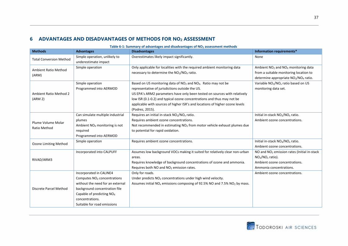
6 ADVANTAGES AND DISADVANTAGES OF METHODS FOR NO2 ASSESSMENT
Table 6-1: Summary of advantages and disadvantages of NO2 assessment methods
Methods Advantages Disadvantages Information requirements*
Total Conversion Method Simple operation, unlikely to
underestimate impact
Overestimates likely impact significantly. None
Ambient Ratio Method
(ARM)
Simple operation Only applicable for localities with the required ambient monitoring data
necessary to determine the NO2/NOX ratio.
Ambient NO2 and NOX monitoring data
from a suitable monitoring location to
determine appropriate NO2/NOX ratio.
Ambient Ratio Method 2
(ARM 2)
Simple operation
Programmed into AERMOD
Based on US monitoring data of NO2 and NOX. Ratio may not be
representative of jurisdictions outside the US.
US EPA’s ARM2 parameters have only been tested on sources with relatively
low ISR (0.1-0.2) and typical ozone concentrations and thus may not be
applicable with sources of higher ISR’s and locations of higher ozone levels
(Podrez, 2015).
Variable NO2/NOx ratio based on US
monitoring data set.
Plume Volume Molar
Ratio Method
Can simulate multiple industrial
plumes
Ambient NOX monitoring is not
required
Programmed into AERMOD
Requires an initial in-stack NO2/NOx ratio.
Requires ambient ozone concentrations.
Not recommended in estimating NO2 from motor vehicle exhaust plumes due
to potential for rapid oxidation.
Initial in-stack NO2/NOx ratio.
Ambient ozone concentrations.
Ozone Limiting Method Simple operation Requires ambient ozone concentrations. Initial in-stack NO2/NOx ratio.
Ambient ozone concentrations.
RIVAD/ARM3
Incorporated into CALPUFF Assumes low background VOCs making it suited for relatively clear non-urban
areas.
Requires knowledge of background concentrations of ozone and ammonia.
Requires both NO and NO2 emission rates.
NO and NO2 emission rates (Initial in-stack
NO2/NOx ratio).
Ambient ozone concentrations.
Ammonia concentrations.
Discrete Parcel Method
Incorporated in CALINE4
Computes NO2 concentrations
without the need for an external
background concentration file
Capable of predicting NOX
concentrations.
Suitable for road emissions
Only for roads.
Under predicts NO2 concentrations under high wind velocity.
Assumes initial NOx emissions composing of 92.5% NO and 7.5% NO2 by mass.
Ambient ozone concentrations.

38
Methods Advantages Disadvantages Information requirements*
Methodologies
developed for DEFRA (UK)
Simple operation
Suitable for road emissions
Only for roads.
May not be representative of jurisdictions outside the UK.
NO2 and NOx monitoring data to develop
the empirical relationship.
Airviro (SE) Simple operation Algorithm may not be representative of jurisdictions outside Sweden. None
Romberg Method (DE)
Simple operation
Incorporated in models such as
PROKAS, IMMIS and MISKAM
May not be representative of jurisdictions outside Germany.
Requires NO2 and NOX monitoring data.
Requires ambient ozone concentrations.
NO2, NOX and ozone monitoring data
required in derivation.
Standard Calculation
Method in the
Netherlands (NL)
Simple operation May not be representative of jurisdictions outside Netherlands.
Applicable for only road applications.
Tends to overestimate by approximately 5 per cent close to the road and
underestimates by approximately 15 per cent away from the road.
Initial NO2 to NOx emission ratio.
Ambient ozone concentrations .
SAPPHO (NL) Simple operation May not be representative of jurisdictions outside Netherlands. None (in Netherlands)
Keller (CH) Simple operation May not be representative of jurisdictions outside Switzerland. None (in Switzerland)
Oxidant Partitioning
Model (UK)
Considers inter-relationships
between NO, NO2 and ozone
Considers source distance
May not be representative of jurisdictions outside UK.
Applicable only to annual average concentrations.
Ambient ozone concentrations.
Limited mixing steady
state approach applied to
annual averages (DE)
May not be representative of jurisdictions outside Germany.
Applicable only to annual average concentrations or in time series
calculations.
Determination of constants for time series calculations can be cumbersome
Applicable for only road applications.
Requires traffic station and background station monitoring data.
NO2, NOx and O3 monitoring data.
Meteorological monitoring data.
Janssen et al (1988)
Simple operation Assumes constant ozone and uses an empirical fit.
Based on empirical data from power plant emissions in the Netherlands.
Ozone concentration, wind speed and
season of the year.
NO2 and NOx concentrations to verify
relationship and constant parameters.
Distance from the source of receptor of
interest.
Photochemistry models
Computer model based
application
Costly, require specialist to operate, may take a long time to run. Highly variable, depending on the
approach.
* It is assumed that basic information needed to describe or quantify the emissions and to model their dispersion in the ambient air is available.

39
7 COMPARISON OF THE ASSESSMENT METHODS FOR USE IN NSW
Table 7-1 presents the summary weighting scales applied in the quantitative evaluation of the NO2
assessment methods.
Table 7-2 to Table 7-3 present an evaluation of each of the potential NO2 assessment methods based
on the following key factors:
Simplicity, meaning the ease of correct use of the method, including by those with limited
specialists skills;
Data requirements, meaning the nature of the data necessary to operate the method, it’s likely
availability, costs and time needed to obtain the data;
Conservatism/ accuracy, meaning the potential scale of any inherent overestimation of the likely
actual impacts. Generally there is a trade-off between the simplicity and data requirements of
a method and its conservatism/ accuracy; and,
Applicability in NSW, an estimate of whether the approach would suit the typical situations
encountered in NSW. This has been considered for urban areas, rural areas and other uses. As
the other uses are generally outside of EPA’s purview, no weighting has been applied, but the
suitability of the method for wider application is indicated with a tick. The applicability of the
methods are determined in the context of emission sector, release type and local environmental
conditions in regard to how the methods are developed or would be adjusted for NSW.
Methods for on-road sources of NO2 are evaluated in a separate table.
Based on the methods’ assumptions, its approach and calculation procedures and the similarity (or not)
between NSW and the localities for which the methods were developed, the likely applicability and
conservatism of the method in NSW was estimated, as shown in the weightings applied in Table 7-2
and Table 7-3.
However, it is not possible within the scope of work for this study to precisely determine the actual
conservatism/ accuracy and applicability in NSW of the majority of the methods. Many of the methods
are developed for specific applications in specific locations outside NSW, thus there are no available
data (e.g. cases of the model use in NSW) to determine whether these methods would be appropriate
and accurate if used in NSW. Thus, such methods are presented in the tables but are not given a
numerical evaluation based on their predictions (conservatism/ accuracy) and applicability in NSW.
The scale for conservatism/ accuracy is non-linear. Assuming accuracy increases on the vertical axis, and
conservatism (overestimation increases on the horizontal axis, the relationship is assumed to be a hump
shape, with maximum accuracy/ conservatism rating of four at the peak of the hump, and lower ratings
lower down either side of the hump. A rating of 1 applies to either end of the base of the hump).

40
Table 7-1: Summary of weighting scales used to evaluate the various NO2 assessment methods
Simplicity
Data requirements
Conservatism/accuracy Applicability i. emission sector ii. release type iii. environmental conditions
1 Very complex 2 Complex 3 Neutral 4 Easy 5 Very easy
1 High 2 Medium 3 Low 4 None beyond minimum
1 Very over or very under conservative and inaccurate 2 Over or under conservative and moderately accuracy 3 Somewhat conservative and accurate 4 Ideally conservative and very accurate
1 Not applicable 2 Applicable in one of three 3 Applicable in two of the three 4 Applicable in all three
Table 7-2: Evaluation of assessment methods for generally all applications
Methods
Sim
plic
ity
Dat
a
req
uir
em
en
t
Co
nse
rvat
ism
/
accu
racy
Applicability in NSW (8)
Tota
l
(22
)
Urb
an
Ru
ral
Oth
er
use
s
(e.g
. ro
ads)
Total Conversion Method 5 4 1 4 4 18
Ozone Limiting Method 4 3 2 4 3 16
Janssen et al (1988) 3 4 3 3 4 - 17
Ambient Ratio Method (ARM) 5 4 2 4 3 18
Ambient Ratio Method 2 4 4 3 4 4 19
Plume Volume Molar Ratio Method
2 3 4 4 4 17
RIVAD/ARM3/ISORROPIA 1 3 - - - - 4
Japan’s exponential function method
2 2 - - - - 4
SAPPHO 3 4 - - - 7
* Most of these methods were developed for their specific jurisdictions. Each method needs to be tested to determine how it
performs in terms of accuracy and conservatism in different applications in NSW. The parameters of the method may also need
to be adjusted to reflect the conditions of NSW or specific region/locality of NSW to where it would be used.
Table 7-3: Evaluation of assessment methods for on-road sources
Methods
Sim
plic
ity
Dat
a
req
uir
em
en
ts
Co
nse
rvat
ism
/
accu
racy
Ap
plic
abili
ty in
NSW
Tota
l
(18
)
Discrete Parcel Method 1 3 3 3 10
Japan’s statistical model 4 4 - - 8
Methodologies developed for DEFRA
(UK) 4 4 - - 8
Airviro (SE) 4 5 - - 9
Romberg Method (DE) 4 3 - - 7
Standard Calculation Method in the
Netherlands (NL) 3 2 - - 5
SAPPHO (NL) 3 5 - - 8
Keller (CH) 4 5 - - 9
Oxidant Partitioning Model (UK)
4 3 - - 7
* Most of these methods were developed for their specific jurisdictions. Each method needs to be tested to determine how it
performs in terms of accuracy and conservatism in different applications in NSW. The parameters of the method may also need
to be adjusted to reflect the conditions of NSW or specific region/locality of NSW to where it would be used.
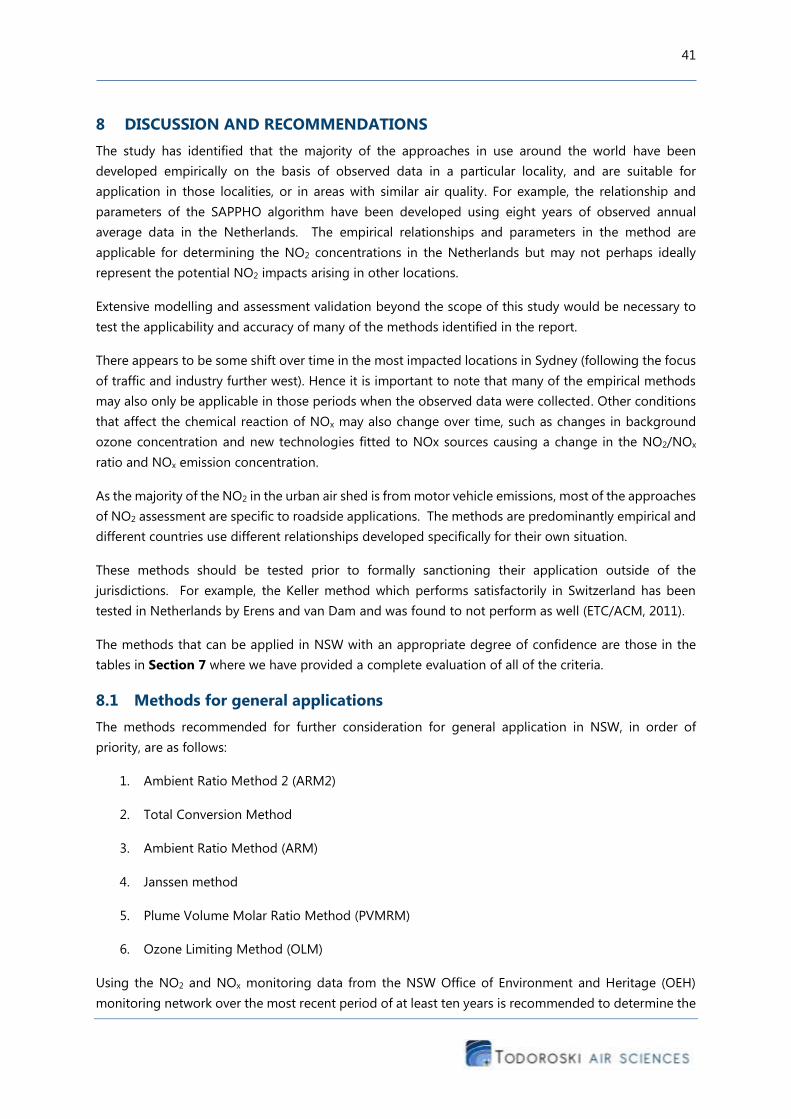
41
8 DISCUSSION AND RECOMMENDATIONS
The study has identified that the majority of the approaches in use around the world have been
developed empirically on the basis of observed data in a particular locality, and are suitable for
application in those localities, or in areas with similar air quality. For example, the relationship and
parameters of the SAPPHO algorithm have been developed using eight years of observed annual
average data in the Netherlands. The empirical relationships and parameters in the method are
applicable for determining the NO2 concentrations in the Netherlands but may not perhaps ideally
represent the potential NO2 impacts arising in other locations.
Extensive modelling and assessment validation beyond the scope of this study would be necessary to
test the applicability and accuracy of many of the methods identified in the report.
There appears to be some shift over time in the most impacted locations in Sydney (following the focus
of traffic and industry further west). Hence it is important to note that many of the empirical methods
may also only be applicable in those periods when the observed data were collected. Other conditions
that affect the chemical reaction of NOx may also change over time, such as changes in background
ozone concentration and new technologies fitted to NOx sources causing a change in the NO2/NOx
ratio and NOx emission concentration.
As the majority of the NO2 in the urban air shed is from motor vehicle emissions, most of the approaches
of NO2 assessment are specific to roadside applications. The methods are predominantly empirical and
different countries use different relationships developed specifically for their own situation.
These methods should be tested prior to formally sanctioning their application outside of the
jurisdictions. For example, the Keller method which performs satisfactorily in Switzerland has been
tested in Netherlands by Erens and van Dam and was found to not perform as well (ETC/ACM, 2011).
The methods that can be applied in NSW with an appropriate degree of confidence are those in the
tables in Section 7 where we have provided a complete evaluation of all of the criteria.
8.1 Methods for general applications
The methods recommended for further consideration for general application in NSW, in order of
priority, are as follows:
1. Ambient Ratio Method 2 (ARM2)
2. Total Conversion Method
3. Ambient Ratio Method (ARM)
4. Janssen method
5. Plume Volume Molar Ratio Method (PVMRM)
6. Ozone Limiting Method (OLM)
Using the NO2 and NOx monitoring data from the NSW Office of Environment and Heritage (OEH)
monitoring network over the most recent period of at least ten years is recommended to determine the

42
appropriate ARM ratio and ARM2 relationship. The development of the appropriate ARM ratio and
ARM2 relationship could follow the method used for their development in the US. One ARM ratio and
ARM2 relationship can be determined for the whole state of NSW. Alternatively, an ARM ratio and
ARM2 relationship for each region (Sydney/Illawarra/etc. or urban/rural) can be developed and applied
in the respective regions.
The use of a single ARM ratio and single ARM2 relationship across the whole state of NSW would require
an ARM ratio and ARM2 relationship that would be conservative enough to use in all regions, but whilst
this would reduce complexity, it may reduce accuracy.
The ARM and ARM2 relationship can be incorporated in current modelling applications which allow
users to modify the source codes. ARM2 values specific for US applications are now incorporated in
AERMOD (Podrez, 2015).
Since air quality impacts are of most concern in the most populated areas, these areas generally have
air quality monitoring data available. Currently, NSW OEH NO2/NOx monitors are located in the Sydney,
Illawarra, Lower Hunter, Upper Hunter and Central Coast regions. As the air quality differs across the
state, it would be more accurate to have an ARM ratio and ARM2 relationship that would differ among
the various regions.
To use the OLM and PVMRM methods, O3 concentration data are needed. Currently, NSW OEH O3
monitors are located in the Sydney, Illawarra, Lower Hunter and Central Coast regions. The assessors
are to justify their use of their chosen O3 concentration data. A conservative fixed O3 concentration
and/or a conservative hourly O3 concentration for an entire year is recommended to be developed for
applications in NSW to be applied in areas where no representative O3 data are available.
A conservative fixed O3 concentration could be set at some percentile of the available O3 monitoring
data across NSW or regions in NSW that would be representative of the maximum O3 concentration
across the state or the specific region in the absence of abnormal conditions. The conservative hourly
O3 concentration for an entire year could be set at a maximum hourly O3 concentrations based on
monitoring data but excluding measurements that may have been caused by abnormal events.
In-stack ratios (ISRs) are also required for the OLM and PVMRM. ISR values should be derived from
source-specific data. Alternatively, data can be obtained from the literature on similar sources.
The other methods, namely RIVAD/ARM3/ISORROPIA, Japan’s exponential function method, SAPPHO,
and Janssen, require evaluation of their performance in predicting NO2 impacts in NSW. Some of the
constant parameters may also need to be adjusted to make them suitable for NSW applications.
Janssen is a currently approved NO2 assessment method in NSW. As the Janssen method was developed
using data from power stations in Netherlands, the method may only be accurate for the situations from
which it was developed (similar to some of the other methods). Evaluation of the method performance
and/or refinement of the method for NSW conditions may be warranted to justify its continued use in
NSW. The use of the Janssen method or its modified form, when verified for NSW, would be appropriate
for application to industries in the GMR.

43
8.2 Methods for on-road sources
Most of the NO2 assessment methods for on-road sources are either empirically-derived or have
scientific basis with empirically-derived parameters. Each method needs to be evaluated for its
performance in predicting NO2 impacts from NSW roads. The equations may also need to be modified
to be suitable for NSW applications. Some of the methods would only allow assessment of NO2 at
longer averaging periods (e.g. annual average).
The Discrete Parcel Method, although not empirically-derived, has some simplified assumptions, and
also needs to be evaluated for NSW applications. The initial NO2/NOx ratio of the vehicle emissions
may also not be appropriate.
The applicable methods listed in Section 8.1 are recommended to be applied for on-road sources.
These methods are more sound, conservative and easier to use.
44
9 REFERENCES
Air Pollution Control Regulations (2004)
Air Pollution Control Regulations, 2004 under the Environmental Protection Act (O.C. 2004-
232), Newfoundland and Labrador Regulation 39/04, May 2004.
The Air Quality (England) Regulations (2000)
The Air Quality (England) Regulations 2000, Statutory Instruments 2000 No. 928, Environmental
Protection, England, enforced on 6 April 2000.
The Air Quality Standards Regulations (2010)
The Air Quality Standards Regulations 2010, Statutory Instruments 2010 No. 1001,
Environmental Protection, enforced on 11 June 2010.
Alberta Environment (2009)
“Air Quality Model Guideline”, Alberta Environment, Government of Alberta, May 2009.
Alberta Environment (2013)
“Alberta Ambient Air Quality Objectives and Guidelines Summary”, Alberta Environment,
Government of Alberta, August 2013.
Alberta ESRD (2012)
Draft Proposed “Air Quality Modelling Guideline”, Alberta Environment and Sustainable
Resource Development, Government of Alberta, November 2012.
AQMAU (2015)
“Conversion Ratios for NOx and NO2”, Air Quality Modelling and Assessment Unit, The
Environment Agency, UK, accessed on May 2015.
http://persona.uk.com/kings_lynn/Core_docs/Q/Q11.pdf
Arizona Department of Environmental Quality (2013)
“Air Dispersion Modeling Guidelines for Arizona Air Quality Permits”, Arizona Department of
Environmental Quality, 23 September 2013.
Atmospheric and Environmental Research (2008)
“CALPUFF Chemistry Upgrade”, prepared by Atmospheric & Environmental Research, Inc., for
American Petroleum Institute.
BC Ministry of Environment (2008)
“Guidelines for Air Quality Dispersion Modelling in British Columbia”, British Columbia Ministry
of Environment, March 2008.
BC Ministry of Environment (2014)
“British Columbia Ambient Air Quality Objectives”, British Columbia Ministry of Environment,
October 2014.
Benson P. (1989)

45
“CALINE4 – A Dispersion Model for Predicting Air Pollution Concentrations Near Roadways”,
Division of New Technology and Research, Department of Transportation, State of California,
June 1989.
CAPCOA (2011)
“Modeling Compliance of The Federal 1-Hour NO2 NAAQS”, California Air Pollution Control
Officers Association, 27 October 2011.
CARB (2011)
“Nitrogen Dioxide – Overview”, California Environmental Protection Agency, Air Resources
Board, last reviewed 21 July 2011.
http://www.arb.ca.gov/research/aaqs/caaqs/no2-1/no2-1.htm
Carslaw, D. (2005)
“Evidence of an increasing NO2/NOx emissions ratio from road traffic emissions”, Atmospheric
Environment 39 (2005) 4793-4802.
Central Pollution Control Board (1994)
“National Ambient Air Quality Standards”, notification S.O. 384(E), Delhi, 11 April 1994.
Central Pollution Control Board (1998)
“National Ambient Air Quality Standards”, notification S.O. 935(E), Delhi, 14 October 1998.
Chu S. H. & Meyer E. L. (1991)
“Use of Ambient Ratios to Estimate Impact of NOx Sources on Annual NO2 Concentrations.” Air
and Waste Management Association 84th Annual Meeting, June 1991. (AWMA Document
Number 91-180.6).
The Clean Air Act (2014)
“Ambient Air Quality Standards”, Appendix to The Clean Air Act, Saskatchewan.
Cole H.S., & Summerhays J.E. (1979)
“A Review of Techniques Available for Estimating Short-Term NO2 concentrations”, Journal of
the Air Pollution Control Association, 29:8, 812-817.
Colorado Department of Public Health and Environment (2015)
“FAQs on Air Quality Modeling Data and Techniques”, v.13July, Colorado Department of Public
Health and Environment, accessed on May 2015.
http://www.colorado.gov/airquality/permits/FAQsOnAirQualityModelingDataAndTechniques1
3Jul.pdf
Düring I., Bächlin W., Ketzel M., Baum A., Friedrich U. & Wurzler S. (2011)
“A new simplified NO/NO2 conversion model under consideration of direct NO2-emissions”,
Meteorologische Zeitschrift, Vol. 20, No. 1, 067-073.
Earth Tech (2000)
“A User’s Guide for the CALPUFF Dispersion Model (Version 5)”, Earth Tech Inc, January 2000.

46
Environmental Protection (Air) Policy (2008)
Environmental Protection (Air) Policy 2008, under Environmental Protection Act 1994,
Queensland, current as at 9 November 2012.
ETC/ACC (2010)
“Guidance on the use of models for the European Air Quality Directive”, ETC/ACC report Version
6.2, European Topic Centre on Air Pollution and Climate Change.
ETC/ACM (2011)
“Guide on modelling Nitrogen Dioxide (NO2) for air quality assessment and planning relevant
to the European Air Quality Directive”, ETC/ACM Technical Paper 2011/15, European Topic
Centre on Air Pollution and Climate Change Mitigation, December 2011.
Ferrari, L. and Salisbury, J. (1997)
“Nitrogen Dioxide”, National Environmental Health Forum Monographs, Air Series No. 3,
National Environmental Health Forum.
Hanrahan P. (1999a)
“The Plume Volume Molar Ratio Method for Determining NO2/NOx Ratios in Modeling – Part I:
Methodology”, Journal of Air and Waste Management Association 49:1324-1331.
Hanrahan P. L. (1999b)
“The Plume Volume Molar Ratio Method for Determining NO2/NOx Ratios in Modeling – Part II:
Evaluation Studies”, Journal of the Air & Waste Management Association, 49:11, 1332-1338.
HK Environmental Protection Department (2015a)
“Guidelines on Choice of Models and Model Parameters”, accessed on May 2015.
http://www.epd.gov.hk/epd/english/environmentinhk/air/guide_ref/guide_aqa_model_g1.html
HK Environmental Protection Department (2015b)
“Air Quality Objectives”, accessed on May 2015.
http://www.epd.gov.hk/epd/english/environmentinhk/air/air_quality_objectives/air_quality_obj
ectives.html
Idriss A. & Spurrell F. (2009)
“Air Quality Model Guideline”, Climate Change, Alberta Environment, Government of Alberta.
Iowa Department of Natural Resources Environmental Services Division (2014)
“Air Dispersion Modeling Guidelines for Non-PSD, Pre-Construction Permit Applications”, Iowa
Department of Natural Resources Environmental Services Division, 19 December 2014.
Janssen L.H.J.M., van Wakeren J.H.A., van Duuren H. & Elshout A.J. (1988)
“A Classification of NO Oxidation Rates in Power Plant Plumes Based on Atmospheric
Conditions”, Atmospheric Environment Vol. 22, No. 1, pp. 43-53, 1988.
Janssen L.M.J.M., Van Haren F., Bange P., & Van Duuren H. (1991)
“Measurements and modelling of reactions of nitrogen oxides in power-plant plumes at night.”
Atmos. Env., 25A, No. 5/6, 829-840.
47
Levitin J., Härkönen J. & Kukkonen J. (2005)
“Evaluation of the CALINE4 and CAR-FMI models against measurements near a major road”,
Atmospheric Environment Volume 39, Issue 25, Pages 4439-4452, August 2005.
Manitoba Government (2005)
“Manitoba Ambient Air Quality Criteria”, Manitoba Government, July 2005.
Moore G.E., Morris R.E., Douglas S.G. & Kessler R.E. (1990)
“Rocky Mountain Acid Deposition Model Assessment: ARM3 Model Performance Evaluation”,
US EPA, Atmospheric Sciences Research Laboratory, Research Triangle Park, NC, June 1990.
Morris R.E., Kessler R.C., Douglas S.G., Styles K.R. & Moore G.E. (1989)
“Rocky Mountain Acid Deposition Model Assessment: Acid Rain Mountain Mesoscale Model
(ARM3)”, US EPA, Atmospheric Sciences Research Laboratory, Research Triangle Park, NC.
National Ambient Air Quality Standards (2009)
National Ambient Air Quality Standards, under National Environmental Management: Air
Quality Act, 2004, Noar. 1210 published in the Government Gazette Staatskoerant, 24 December
2009.
National Regulations Regarding Air Dispersion Modelling (2014)
National Regulations Regarding Air Dispersion Modelling, under National Environmental
Management: Air Quality Act, 2004, No. R. 533 published in the Government Gazette
Staatskoerant, 11 July 2014.
Newfoundland and Labrador DEC (2012)
“Guideline for Plume Dispersion Modelling”, Department of Environment and Conservation,
Government of Newfoundland and Labrador, September 2012.
Nguyen L. & Wesseling J.P. (2008)
“OSPM: Comparison between modelled results obtained for the Erzeijstraat in the Netherlands
and measurements”, RIVM Report 680705011/2008, National Institute for Public Health and
Environment, Netherlands.
NHMRC (2008)
“Air Quality In and Around Traffic Tunnels”, National Health and Medical Research Council,
Commonwealth of Australia.
NSW DEC (2005)
“Approved Methods for the Modelling and Assessment of Air Pollutants in NSW”, August 2005.
NSW DECC (2009)
“Interim DECC Nitrogen Oxide Policy for Cogeneration in Sydney and the Illawarra”, Department
of Environment and Climate Change NSW, February 2009.
http://www.environment.nsw.gov.au/resources/air/inp09124.pdf
NSW DECCW (2010a)
“Current air quality in New South Wales – A technical paper supporting the Clean Air Forum
2010”, Department of Environment, Climate Change and Water NSW, August 2010.

48
NSW DECCW (2010b)
“State of Knowledge: Ozone”, State of NSW and Department of Environment, Climate Change
and Water NSW, September 2010.
NYS DEC (2006)
“NYSDEC Guidelines on Dispersion Modeling Procedures for Air Quality Impact Analysis”, DEC
Program Policy, New York State Department of Environmental Conservation, 9 May 2006.
NSW EPA (2012a)
“Tracking sources of air pollution in NSW communities – Air emissions inventory for the Greater
Metropolitan Region of NSW”, Environment Protection Authority, State of NSW, August 2012.
NSW EPA (2012b)
“2008 Calendar Year Air Emissions Inventory for the Greater Metropolitan Region in New South
Wales – On-Road Mobile Emissions: Results”, Environment Protection Authority, State of NSW,
August 2012.
NSW EPA (2012c)
“2008 Calendar Year Air Emissions Inventory for the Greater Metropolitan Region in New South
Wales – Industrial Emissions: Results”, Environment Protection Authority, State of NSW, August
2012.
NZ Ministry for the Environment (2004)
“Good Practice Guide for Atmospheric Dispersion Modelling”, prepared by the National
Institute of Water and Atmospheric Research, Aurora Pacific Limited and Earth Tech
Incorporated for the Ministry of the Environment, June 2004.
NZ Ministry for the Environment (2008a)
“Good Practice Guide for Assessing Discharges to Air from Industry”, Ministry for the
Environment, May 2008.
NZ Ministry for the Environment (2008b)
“Good Practice Guide for Assessing Discharges to Air from Land Transport”, Ministry for the
Environment, June 2008.
Ohio EPA (2014)
“Engineering Guide #69: Air Dispersion Modeling Guidance”, Ohio Environmental Protection
Agency, July 2014.
http://epa.ohio.gov/Portals/27/sip/document/2014-07-17%20FINAL%20Revised%20EG69.pdf
OLM/ARM Workgroup (1998)
Draft Recommendations “Use of the Ambient Ratio Method (ARM) for Estimating Ambient
Nitrogen Dioxide Concentrations”, prepared by the OLM/ARM Workgroup, May 1998.
https://dec.alaska.gov/air/ap/docs/sitearm.pdf
Ontario Ministry of the Environment (2009)
“Air Dispersion Modelling Guideline for Ontario”, Version 2.0, Ontario Ministry of the
Environment, March 2009.
Ontario Ministry of the Environment (2012)
“Ontario’s Ambient Air Quality Criteria”, Ontario Ministry of the Environment, April 2012.

49
Overseas Environmental Cooperation Center (1998)
“Air Pollution Control Technology Manual”, FY 1997 project for the advisement of Sustainable
Development Support commissioned by Environment Agency, Government of Japan, Overseas
Environmental Cooperation Center, March 1998.
People’s Republic of China (1996)
“Ambient Air Quality Standard”, Document in Chinese.
Podrez M. (2012)
“Updated Tier 2 Ambient Ratio Method (ARM) for 1-hr NO2 NAAQS Analyses”, prepared by
Mark Podrez of RTP Environmental Associates at the EPA’s 10th Modeling Conference, 14 March
2012.
http://www.epa.gov/scram001/10thmodconf/presentations/2-12-
ARM2_Presentation_for_EPA_10th_Modeling_Conference_-_3-12-2012.pdf
Podrez M. (2015)
“An update to the ambient ratio method for 1-h NO2 air quality standards dispersion modeling”,
Atmospheric Environment 103 (2015) 163-170.RTP Environmental Associates (2013)
Québec Ministère du Développement durable, de l’Environnement et Parcs (2005)
“Guide de la Modélisation de la Dispersion Atmosphérique”, Québec Ministère du
Développement durable, de l’Environnement et Parcs, Avril 2005.
Québec Ministère du Développement durable, de l’Environnement et Parcs (2008)
“Guide D’Estimation de la Concentration de Dioxyde D’Azote (NO2) Dans l’Air Ambiant Lors de
l’Application des Modèles de Dispersion Atmosphérique”, Québec Ministère du Développement
durable, de l’Environnement et Parcs, Août 2008.
Québec Ministère du Développement durable, de l’Environnement et Parcs (2010)
“Mise à jour des critères québécois de qualité de l’air”, Québec Ministère du Développement
durable, de l’Environnement et Parcs, Mars 2010.
Rhode Island Department of Environmental Management (2013)
“Rhode Island Air Dispersion Modeling Guidelines for Stationary Sources”, State of Rhode
Island, Department of Environmental Management, Office of Air Resources, March 2013.
RTP Environmental Associates (2013)
“Ambient Ratio Method Version 2 (ARM2) for use with AERMOD for 1-hr NO2 Modeling –
Development and Evaluation Report”, prepared by RTP Environmental Associates, Inc. for
American Petroleum Institute, September 2013.
SA EPA (2006)
“EPA Guidelines – Air quality impact assessment using design ground level pollutant
concentrations (DGLCs)”, Environment Protection Authority, Government of South Australia,
updated January 2006.
Saskatchewan Ministry of Environment (2012)

50
“Saskatchewan Air Quality Modelling Guideline”, Saskatchewan Ministry of Environment,
Government of Saskatchewan, March 2012.
South Africa’s Department of Environmental Affairs (2014)
Code of Practice for Air Dispersion Modelling in Air Quality Management in South Africa, 2014,
Department of Environmental Affairs, Republic of South Africa.
State Environment Protection Policy (Ambient Air Quality) (1999)
State Environment Protection Policy (Ambient Air Quality), under Environment Protection Act
1970, published in the Victoria Government Gazette, No. S 19, 9 February 1999.
State Environment Protection Policy (Air Quality Management) (2001)
State Environment Protection Policy (Air Quality Management), under Environment Protection
Act 1970, published in the Victoria Government Gazette, No. S 240, 21 December 2001.
TAS (2015)
“Air Quality Considerations – Proposed Badgerys Creek Airport”, presentation by Aleks
Todoroski of Todoroski Air Sciences for the Penrith Council, 2015.
Texas Commission on Environmental Quality (2014)
“Air Quality Modeling Guidelines”, APDG 6232, Air Permits Division, Texas Commission on
Environmental Quality, June 2014.
UK Environment Agency (2007)
“Review of methods for NO to NO2 conversion in plumes at short ranges”, Environment Agency,
UK.
US EPA (2005)
40 CFR Part 51 “Revision to the Guidelines on Air Quality Models: Adoption of a Preferred
General Purpose (Flat and Complex Terrain) Dispersion Model and Other Revisions” Final Rule,
US EPA, November 2005.
US EPA (2010a)
“Applicability of Appendix W Modeling Guidance for the 1-hour NO2 National Ambient Air
Quality Standard”, US EPA Memo, 28 June 2010.
US EPA (2010b)
“Guidance Concerning the Implementation of the 1-hour NO2 NAAQS for the Prevention of
Significant Deterioration Program”, US EPA Memo, 29 June 2010.
US EPA (2011)
“Additional Clarification Regarding Application of Appendix W Modeling Guidance for the 1-
hour NO2 National Ambient Air Quality Standard”, US EPA Memo, 1 March 2011.
VIC EPA (2013)
“Guidance notes for using the regulatory air pollution model AERMOD in Victoria”, Publication
1551, EPA Victoria, October 2013.

51
Wang Y.J., DenBleyker A., McDonald-Buller E., Allen D., & Zhang K. (2011)
“Modeling the chemical evolution of nitrogen oxides near roadways”. Atmos. Env., 45, 43-52.
Weiss M., Bonnel P., Kühlwein J., Provenza A., Lambrecht U, Alessandrini S., Carriero M., Colombo R.,
Forni F., Lanappe G., Le Lijour P., Manfredi U., Montigny F. and Sculati M. (2012)
“Will Euro 6 reduce the NOX emissions of new diesel cars? – Insights from on-road tests with
Portable Emissions Measurement Systems (PEMS)”. Atmos. Env., 62, 657-665.