assessing the timber situation in georgia using the …

ASSESSING THE TIMBER SITUATION IN GEORGIA USING THE MULTI-PRODUCT

SUBREGIONAL TIMBER SUPPLY (MP-SRTS) MODEL: 2005-2025

by

VERNON WESTON HIOTT

(Under the Direction of Michael L. Clutter)

ABSTRACT

The development of the Multi-Product Subregional Timber Supply Model (MP-SRTS)

has expanded the ability to precisely project future quantities of raw forest products. Developed

from the Subregional Timber Supply Model (SRTS), MP-SRTS allows projections to be made

on a product basis. The ability to differentiate among product classifications has allowed

declined demand levels for forest products to be examined by product. Using MP-SRTS allows

market conditions to be assessed more precisely and provides a better understanding of the future

regional outlook for raw forest products within the state of Georgia. The State is projected to

experience depressed levels of raw forest product inventory with stable harvest levels and

increasing upward pressure on raw forest product prices. The largest reduction in raw forest

product inventory is projected to occur in the North Central FIA survey unit and documents the

continued impact of land use change surrounding Atlanta, Georgia.

INDEX WORDS: MP-SRTS, Forest Market Modeling, Timber Product Supply, Supply and

Demand, Georgia, Timber Price



by

VERNON WESTON HIOTT

B.S., Clemson University, 2004

A Thesis Submitted to the Graduate Faculty of

The University of Georgia

in Partial Fulfillment of the Requirements for the Degree

MASTER OF SCIENCE

ATHENS, GEORGIA

2006

© 2006

Vernon Weston Hiott

All Rights Reserved



by

VERNON WESTON HIOTT

Major Professor: Michael L. Clutter

Committee: Bruce E. Borders Jacek P. Siry

Electronic Version Approved: Maureen Grasso Dean of the Graduate School The University of Georgia August 2006

DEDICATION

To my father, Craig Hiott, for instilling in me the drive and determination to achieve my

goals, and to my mother, B.J. Hiott for her endless support, love and encouragement.

iv

ACKNOWLEDGEMENTS

My major professor, Dr. Michael L. Clutter, deserves thanks for providing guidance

during this project and for introducing me to many academic concepts that have influenced my

professional life. My committee members, Dr. Bruce E. Borders and Dr. Jacek P. Siry who have

helped with this project and have taught me so much.

I also extend thanks to my family and friends for all the support they have given me.

Their encouragement throughout the past year and a half is greatly appreciated.

v

TABLE OF CONTENTS

Page

ACKNOWLEDGEMENTS.............................................................................................................v

LIST OF TABLES........................................................................................................................ vii

LIST OF FIGURES ..................................................................................................................... viii

CHAPTER

1 Introduction and Literature Review...............................................................................1

Model Development ..................................................................................................6

Current Trends.........................................................................................................10

2 Methods........................................................................................................................18

Market Module ........................................................................................................19

Inventory Module ....................................................................................................22

Model Scenario........................................................................................................24

3 Results..........................................................................................................................27

4 Conclusions..................................................................................................................43

REFERENCES ..............................................................................................................................45

vi

LIST OF TABLES

Page

Table 1: MP-SRTS Model Softwood Projections by Region ........................................................31

Table 2: MP-SRTS Model Hardwood Projections by Region.......................................................33

vii

LIST OF FIGURES

Page

Figure 1: Georgia Statewide Quarterly Real Stumpage Prices......................................................11

Figure 2: Georgia Statewide Quarterly Percent Change in Pine Product Prices ...........................12

Figure 3: Georgia Statewide Quarterly Percent Change in Hardwood Product Price ...................13

Figure 4: Georgia Softwood Timber Product Output ....................................................................15

Figure 5: Georgia Hardwood Timber Product Output...................................................................15

Figure 6: Forest Service Survey Units for Georgia .......................................................................19

Figure 7: MP-SRTS Market Module .............................................................................................20

Figure 8: MP-SRTS Inventory Module .........................................................................................23

Figure 9: State level hardwood and softwood inventory shifts by product ...................................28

Figure 10: State level hardwood and softwood growth shifts by product .....................................28

Figure 11: State level hardwood and softwood removals by product............................................29

Figure 12: State level raw forest product prices by product ..........................................................29

Figure 13: Softwood inventory shifts by FIA survey unit .............................................................35

Figure 14: Hardwood inventory shifts by FIA survey unit............................................................35

Figure 15: Softwood growth shifts by FIA survey unit .................................................................36

Figure 16: Hardwood growth shifts by FIA survey unit................................................................37

Figure 17: Softwood removals by FIA survey unit .......................................................................38

Figure 18: Hardwood removals by FIA survey unit ......................................................................38

Figure 19: Raw timber product price projections for the Northern survey unit ............................40

viii

Figure 20: Raw timber product price projections for the North Central survey unit.....................41

Figure 21: Raw timer product price projections for the Central survey unit .................................41

Figure 22: Raw timber product price projections for the Southeastern survey unit ......................42

Figure 23: Raw timber product price projections for the Southeastern survey unit ......................42

ix

Chapter 1

Introduction and Literature Review

The southern United States produces more timber than any single country in the

world and is projected to remain the dominant producing region for many decades to

come (Prestmon and Abt, 2003). The U.S. South produces approximately 15% of the

industrial roundwood in the world (Smith et al. 2004). The ability to produce this amount

of raw forest products can be contributed in large part to loblolly pine (Pinus taeda L.),

the most economically significant timber species in the world. The range of loblolly pine

reaches across the Atlantic and Gulf Coastal Plains from eastern Texas to southern

Maryland (Wahlenberg, 1960). Loblolly pine in this region consists of more than 68

billion cubic feet in total growing stock (Haynes, 1990).

Loblolly pine is becoming an increasingly important species in Southern forests

as acreage under intensive management increases. During the past thirty years, pine

plantation acres have surpassed natural pine acres; hence loblolly pine plantations have

become the major source of raw forest products (Cost, 1989). As of 2005, the U.S. South

is estimated to contain 177.4 million acres of forestland of which 37.8 million acres

supports pine plantations (Cubbage et al., 2006).

Forestland ownership in the Southern United States is composed of three major

groupings: private industrial, non-industrial private, and public. The South produces

approximately 60 percent of the Nation’s timber products and almost all of it originates

from private forests (Prestmon and Abt, 2003). Private forestland owners control 93% of

1

the South’s forestland with only 7% being under public control. Within the 93% that is

privately held, forest industry controls 32% and non-industrial private forestland owners

(NIPFs) hold 61% (Siry et al., 2005). The U.S. South has the largest concentration of

both industrial ownership and non-industrial private ownership in the United States

(Clutter et al., 2005).

Non-industrial private forestland owners control the vast majority of forestland in

the Southern U.S. with approximately 110.2 million acres (Cubbage et al., 2006). NIPFs

are a diverse group of forestland owners with a wide array of timberland management

objectives. Members include individuals, family trusts, and S-corporations created to

hold timberland assets. The NIPF ownership classification is expected to become even

more important as ownership trends continue to favor private ownership over C-

corporations (Clutter et al., 2005). Birch (1996a and b) found that within the U.S. South

55% of the forestland controlled by NIPFs had a financially based primary management

objective with 35% being to produce timber. Many NIPFs hold forestland as part of a

larger land holding such as farmland. In these instances the forestland owner may not

view timber management as a primary source of income as owners holding only

forestland. The inventory distribution by management type somewhat reflects this across

the South. For NIPFs throughout the Southern U.S. the majority of forestland is held in

upland hardwood, approximately 42% or 45.7 million acres. Pine plantations under

NIPF ownership only comprise around 12.4% or 13.5 million acres, but these plantations

are not completely uniform monocultures due to their contributing 2.3% of the annual

hardwood timber removals (Cubbage et al., 2006).

2

The forest industry within the Southern U.S. is a management intensive, ever

evolving class of forestland owners. Southern U.S. forestland controlled by the forest

industry is approximately 56.6 million acres and is composed of 22.7 million acres of

pine plantation (Cubbage et al., 2006). The pine plantation component of forest industry

holdings represents 40% of the ownership and reflects the emphasis that is placed on

property to maximize return with intensively managed plantations and also provide a

consistent source of raw forest products to manufacturing facilities. Recent trends have

documented a realization by forest industry that wood can be procured continually on the

open market and has spawned movement of forest ownership away from this ownership

class. From 1996 through 2004 the Southern U.S. experienced movement of 18.4 million

acres, the majority of which transferred ownership from forest industry entities to

institutional ownership (Clutter et al., 2005). The implications for future timber supplies

are unclear at present; however, by examining the relative intensity of NIPF management,

impacts are likely to be negative.

Public ownership of timberland rarely identifies timber production as a primary

management objective. In the Southern U.S. public ownership accounts for only 7% of

the forestland base and of that 7%, only 11% is held as pine plantations (Cubbage et al.,

2006). The management of public forestland in not primarily aligned with financial

principles and therefore is not considered as a significant participant within the forest

sector. In addition, when considering future projections that are based on economic

factors, the modeling assumptions are not appropriate and therefore public holdings are

not examined as a source of future timber supply (Prestmon and Abt, 2003).

3

Similar to the region, the State of Georgia follows the Southern U.S. in forestland

significance and structure. In 2001, Georgia’s forest products industry employed

approximately 204,000 workers, produced an economic output of over $19 billion, and

supported approximately $30.5 billion in economic activity (Riall, 2002). The economic

output of the forest sector represents the direct influence of the industry on the State’s

economy. The $19 billion is created by the operations and transactions related to the raw

forest products. Economic activity resulting from the forest sector amounted to $30.5

billion and is the secondary dispersion of value back into the State’s economy, for

instance, lumber being sold at a home improvement store or a forest industry employee

spending an earned salary. Clearly, the forest industry has a substantial impact on the

economic health of Georgia.

Investment within the forest product sector can be a primary force for growth and

new development across the State. Identifying potential investment opportunities,

whether for an individual purchasing timberland or an industrial entity establishing or

expanding a mill requires careful consideration of current and future raw materials

market conditions. The ability to predict these future relationships is central to business

planning and investment analysis. Assessing the raw material needs of the industry and

predicting the future quantities of these materials is crucial in supporting sustainable

operations and maintaining a healthy forest products sector.

Investment analysis is also used when applying stand level silvicultural

treatments. Silvicultural activities should be justified by producing a sufficient marginal

return. Price fluctuations influence the realized return resulting from silvicultural

applications, and depressed prices result in lower silvicultural investment particularly for

4

non-industrial private forestland owners. Decreased levels of stand investment result in

lower stand production rates and consequently lower supplied levels of raw forest

products in the market place. The ability to reflect these production declines in market

modeling better equips members within the forest sector when formulating a long-term or

strategic plan.

Forecasting timber conditions for the projection period requires projecting

growth, inventory and harvest in the market on an annual basis. The initial point of the

projection period is described as having an established inventory level. This supply level

determines the starting point upon which the following year’s characteristics are

calculated. With the initial inventory established, the annual harvest is applied along

with the amount of growth over the year. At the end of the year, deducting the harvest

and adding the growth to the initial inventory, calculates the net movement in timber

inventory levels. Based on the amount of timber available for harvest and the harvest

level, a price is determined for each product for the year. The calculated price for the

year influences the quantity and distribution of timberland acreage and the assignment of

pine plantation acreage for the area being analyzed. This process is repeated for each

year in the projection period.

One of the major components in expanding the market conditions from the initial

point to the end of the projection period is the amount of growth that is accomplished

over the course of each individual year. The growth of timber is a function of many

factors including the current price level of forest products in the market. In order to

capture the effect of depressed price levels in the projection, adjustments are made to the

annual growth rates applied to the timber inventory level. Due to recent depressed price

5

levels for timber products, as shown in Figure1, this analysis provides an understanding

of the influence of current price levels on projected market conditions for raw forest

products.

Model Development:

Timber supply, demand and price trends have been evaluated for the nation and

for the South (Haynes, 2003; Prestmon and Abt, 2003). Forest modeling has evolved

from multiple state inventory approaches such as the Aggregate Timberland Assessment

System, or ATLAS, to representing subregional inventory and economic implications

based on products as with the Multi-Product Subregional Timber Supply model (MP-

SRTS). Initial modeling attempted and achieved the ability to represent aggregate

inventory levels for a multi-state region such as the Southern United States. As

shortcomings were identified and models were developed to include factors such as land

use change, economic conditions, and product classifications.

An initial challenge was the vast areas of forestland that were analyzed as a

consistent group or strata in such inventory projection models. Projections were made on

a regional basis where the regions included several states grouped together. This

approach assumes that species, growth, and market behavior remain constant over the

entire region. Without question these factors vary within a single state and are much less

likely to remain unchanged over a multi-state region. The market presence is likely to be

the most varying factor within an area. Market presence is the demand for raw forest

products in a particular area. Depending on the number and capacity of processing

centers in the area, pressure placed on the inventory by product varies. As processing

capacity increases the pressure applied to the surrounding inventory is increased.

6

Consequently in this situation the area will experience a real increase in the price of the

demanded raw material.

The Aggregate Timberland Assessment System-ATLAS was developed by the

U.S. Forest Service and used in conjunction with the 1989 Renewable Resource Planning

Act. The model was developed to address a broad range of policy questions related to

future timber supplies (Mills and Kincaid, 1992). Renewed concern in the potential of

consuming the country’s forest resources fueled the development and use of ATLAS as

an evaluation tool for the forest resources in the United States.

The ATLAS system employs aggregate estimates of inventory, harvest and

growth at various, but course, levels of resolution to describe the region. The inventory

data is collected at the U.S.F.S. Forest Inventory and Analysis survey unit level and

combined to describe the region where the harvest is applied. The model covers a broad

area that is considered as having homogenous growth and market characteristics.

The primary input modules are inventory, management and harvest. The

inventory component establishes the base level of resources available by acre and volume

per acre by age class. This measure sets the base upon which to develop forecasts.

Geographic region, owner, forest type, site and other factors categorize the acreage and

volume per acre quantities. The total inventory for the region is found by combining the

established inventory units that are at a more specific level of resolution. Within the

individual inventory units, five management classifications are applied which reflect

differences in management intensity. The management assignment includes:

regeneration, growth and harvest variables that simulate stand improvement, management

alternatives and area change characteristics. The management component can vary in the

7

levels of each variable applied to simulate differences in species composition. This

allows several stand situations to be represented with varying degrees of management

intensity. The inventory units with management scenarios applied are assigned a harvest

level that is distributed among the separate inventory units.

The ATLAS model approach allows the forest resources for the region to be

assessed and projected based on the established base, assigned growth and yield rates,

and by given levels of harvests. The use of aggregate data allows a prediction to be

formed for the region has a whole but for no smaller resolution and ATLAS lacks product

resolution as well. The applications of the model results are limited due to the large area

that is included and the lack of product specificity.

In order to be more specific and concentrate on the State of Georgia’s timber

situation the Georgia Regional Inventory Timber Supply or GRITS, was developed to

gain understanding regarding the timberland resources within the state of Georgia. The

model uses each of five regions defined by the USDA Forest Service FIA as reporting

levels. GRITS uses estimates from the USDA Forest Service FIA database, which

presents timber inventory by region within the state. The Forest Inventory and Analysis

(FIA) database supplies levels of timberland area, timberland inventory, timber growth

rates, and timber removals (Abt et al., 2000). Using the supplied information GRITS

computes the future levels of timber available within the five regions in Georgia.

The GRITS model expands on the capabilities of ATLAS by being more specific

to a particular area that may perform more similar to a homogeneous unit. This inventory

model provides a methodology for predicting future timber supply based on existing

inventories, management intensities (representing ownership), and current and future

8

harvest levels. A primary flaw in using GRITS is that the current harvest level represents

demand and is adjusted over time by anticipated movements in that harvest level. In

addition, shifts in land area under management are exogenous to the model. The GRITS

model allows the resources for the state of Georgia to be assessed independently from

other states in the Southeastern United States.

Expanding on the GRITS inventory model, the Subregional Timber Supply

(SRTS) model was developed to incorporate impacts from market conditions. The Sub-

Regional Timber Supply model is widely used and accepted for projecting supply,

demand and price trends in the South (Prestmon and Abt, 2003). SRTS was initially

developed at North Carolina State University to provide the southern United States with a

model that did not consider the area as a homogenous timber-producing sector as did

previous models (e.g. ATLAS), but rather a diverse region composed of subunits that

contain wide variation in market conditions (Mills and Kincaid, 1992; Prestmon and Abt,

2003). SRTS provides an economic overlay to traditional inventory models. These

market conditions drive the determination of timberland allocation by area and

management type. The SRTS model applies economic conditions to inventory models

and has been used in conjuncture with both the ATLAS and GRITS models. SRTS

provides useful projections that are specific by region; however, the model does not have

the capability to capture movements based on specific raw materials product categories.

To address product movements individually, the Multi-Product Subregional

Timber Supply (MP-SRTS) model was developed. The MP-SRTS model is a partial-

equilibrium timber market simulation model, and is used to analyze various forest

resource and timber supply scenarios (Abt et al., 2000). The MP-SRTS model provides a

9

tool for examining timber conditions in light of multiple product classifications, land

conversion or land use change, and management intensity. The major implication of

using the MP-SRTS model is that this model is capable of classifying values based on

more descriptive product classes, such as pine pulpwood or hardwood sawtimber, as

opposed to SRTS classifications of growing stock and inventory by hardwood and

softwood classes.

The classifications based on product class and species group allow projections to

be made that identify fluctuations not only in the inventory level as a whole, but as

individual product classes. Separating values by product class allows information to be

provided that is particular to specific area and user. For instance, a pulp and paper

manufacturer would be provided with projected hardwood and softwood pulpwood

values separate from sawtimber projections. Additionally, this model allows

interdependencies between product classes to be simulated. For example, the quantity of

hardwood pulpwood used to produce pulp is directly related to the amount of softwood

pulpwood used as a substitute and is, therefore, indirectly related to softwood sawtimber

harvest in any given year. These projections will be more relevant to many users than

those previously provided by the Southern Forest Resource Assessment, which was based

on the SRTS model (Prestemon and Abt, 2003).

Current Trends

The MP-SRTS model will be used to predict values of timber market conditions

and timberland allocation in Georgia from 2005 to 2025. These projections will reflect

recent trends in raw forest product prices in Georgia, particularly pine pulpwood, and

steadily increasing hardwood stumpage costs, as shown in Figure 1. Considering these

10

price trends and associated timber product output levels presented below, market

responses are sure to occur.

0

10

20

30

40

50

60

1985

1986

1987

1988

1989

1990

1991

1992

1993

1994

1995

1996

1997

1998

1999

2000

2001

2002

2003

2004

2005

$/To

n

Pine PW Pine CNS Pine Saw Hd PW Hd Saw

Figure 1. Georgia Statewide Quarterly Real Stumpage Prices Source: Timber-Mart South, 2006

Since 2002, pine pulpwood prices have remained at levels not seen since 1989.

Similarly, pine chip-n-saw and sawtimber have both experienced price declines following

strong levels during the late 1990s and early 2000. Pine sawtimber prices have

strengthened after a substantial reduction during 2000 and 2001. In contrast, hardwood

pulpwood and hardwood sawtimber prices have experienced an upward trend.

Figures 2 and 3 present the statewide quarterly price movements as percentages

and show the fluctuation in the volatility of the timber product prices. Throughout the

1990s, timber product prices fluctuated drastically before settling and becoming more

stable after 2000. Pine product prices, as shown in Figure 2, became less volatile after

11

2002. The pine product prices move in the same direction annually; however, the

severity in movements by product varies with pine pulpwood being most volatile.

-35%

-25%

-15%

-5%

5%

15%

25%

35%

1985

1986

1987

1988

1989

1990

1991

1992

1993

1994

1995

1996

1997

1998

1999

2000

2001

2002

2003

2004

2005

Pine Pulp Pine CNS Pine Saw

Figure 2. Georgia Statewide Quarterly Percent Change in Pine Product Prices Source: Timber-Mart South, 2006

The quarterly price movements for hardwood product prices are presented in

Figure 3 and document that hardwood product prices have historically been more volatile

than softwood products. Over the last twenty years, hardwood product price variability

has been greatest in the early to mid nineties. More recent movements, from 2003 to the

first quarter of 2006, have witnessed a heightened level of variability as compared to the

2000 to 2003 period. As with the softwood product prices, hardwood pulpwood

experiences more movement than sawtimber.

12

-35%

-25%

-15%

-5%

5%

15%

25%

35%

45%

55%

65%

1985

1986

1987

1988

1989

1990

1991

1992

1993

1994

1995

1996

1997

1998

1999

2000

2001

2002

2003

2004

2005

Hardwood Sawtimber Hardwood Pulpwood

Figure 3. Georgia Statewide Quarterly Percent Change in Hardwood Product Price Source: Timber-Mart South, 2006

Forest managers and owners relate the volatility in product prices as risk. As the

volatility of these product prices increases, the amount of risk assumed by management is

heightened. Management may be altered to limit the assumed risk, which would impact

stand development and growth negatively. Deferring stand treatments or substituting

with less costly and less effective methods will not allow growth potentials on sites to be

realized. The implication of less silvicultural investment across the State is a significant

reduction in total forest product supplied to the market. The reduction in supply resulting

from increased levels of harvest and declines in growth rates will cause stumpage prices

to increase.

13

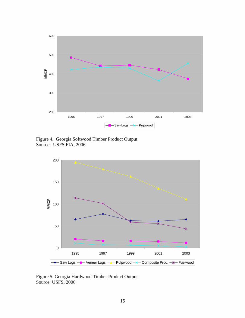
As seen in Figure 4, initial production rates were unresponsive to price shifts for

pulpwood from 1999 to 2001; however, during 2003 pulpwood production levels

increased by approximately 100 million cubic feet. Sawtimber production responded to

increasing prices as product output declined by approximately 75 million cubic feet from

1999 to 2003 (USFS, 2006). These product output trends will lead to lower sawtimber

prices and increased stumpage cost for pine pulpwood. Other product output levels of

composite products have increased by approximately 6 million cubic feet among the four

composite panel, or oriented strand board, mills in Georgia (Johnson and Wells, 2005).

The increased production is obviously related to the decline in stumpage of pine

pulpwood and chip-n-saw. Relative to saw logs and pulpwood, all other softwood

products have remained stable with little variation.

Hardwood trends are similar in being responsive to price levels; however,

hardwood prices have steadily strengthened from 1995 to 2003 and with the exception of

slight growth in hardwood sawtimber output, hardwood product output has declined. As

seen in Figure 5, hardwood pulpwood has declined most dramatically with a fifty million

cubic foot reduction in product output. Much of this decline can be contributed to the

increase in pine pulpwood output as a substitute and limited supplies of hardwood fiber.

14

200

300

400

500

600

1995 1997 1999 2001 2003

MM

CF

Saw Logs Pulpwood

Figure 4. Georgia Softwood Timber Product Output Source. USFS FIA, 2006

0

50

100

150

200

1995 1997 1999 2001 2003

MM

CF

Saw Logs Veneer Logs Pulpwood Composite Prod. Fuelwood

Figure 5. Georgia Hardwood Timber Product Output Source: USFS, 2006

15

The movements in prices heavily influence management decisions, particularly,

silvicultural practices. Additionally, price declines reduce the feasibility of retaining

certain acreage in timber management and management intensity. An increasing factor

that magnifies reductions in the timberland base has been coined as urban sprawl. The

Southern Forest Resource Assessment has indicated that urban sprawl has a major impact

on the operations of the forest sector and contributes to losses in southern United States

timberland (Prestmon and Abt, 2003). Urbanization has a significant impact on average

parcel size and if present trends continue, by the year 2010 approximately 95% of the

nation’s private forest ownership will be in parcels of less than 100 acres (Mehmood and

Zhang, 2001; DeCoster, 1998). This increase of owners holding fewer acres is known as

parcelization and generally leads to fragmentation and timberland loss (Mehmood and

Zhang 2001). The implication for the State of Georgia is important when considering

development hotbeds within the State such as areas in and around Atlanta.

Parcelization influences management activities in that the feasibility of

silvicultural applications is related to the treatment unit’s size. The affect of parcelization

is two-fold. Not only is timberland lost as a direct effect of new owner objectives being

outside of timber management but also through the loss of management options that were

viable on the original, larger, tract. In Mississippi and Alabama, proximity to

development and more densely populated areas almost always led to lower harvesting

rates (Barlow et al., 1998). The implication is that with limited management options,

acreage will more rapidly experience land use change or will provide less than optimum

levels of return.

16

Timberland forms the base of an actively growing and contributing sector within

the State. The forest sector provides substantial monetary and social benefits and will

continue to be a strong industry. Modeling techniques have been developed to forecast

market conditions that can aid in planning and investment. Using the MP-SRTS model

the current low price levels can be reflected in these projections to predict the impacts on

future levels of supply, demand and price of forest products and the acreage under timber

management.

17

Chapter 2

Methods

The Multi-Product Subregional Timber Supply model, like SRTS, provides an

economic component to inventory models; however, the implications are examined for

each product. The use of MP-SRTS provides results that are specific to each state survey

unit. This geographical scope allows variation to be captured across the State of Georgia

and among separate market baskets within the State. Figure 6 shows the subregional

survey units that will act as reporting levels to assist in delineating separate timber

markets across the State. MP-SRTS works similar to many inventory models that

consider a particular harvest scenario and allows conditions including potential price

consequences, subregional harvest shifts, and inventory fluctuations to be represented

consistently.

MP-SRTS is applicable to several inventory models including ATLAS and

GRITS. The inventory module used for this analysis was modeled after the GRITS

model (Cubbage et al. 1990). The inventory and market modules are the two major

modeling components. Beginning with the market, which is composed of the subregional

survey units, the base price equilibrium is calculated using various market statistics.

Subregional movements in price and inventory are used to determine the distribution of

harvest intensity by subregion. Within Georgia there are five FIA survey units, as shown

in Figure 6, and when analyzed by forest industry and NIPF owners there are ten separate

owner / areas that exist in the model (5 subregions * 2 ownership classes). As discussed

18

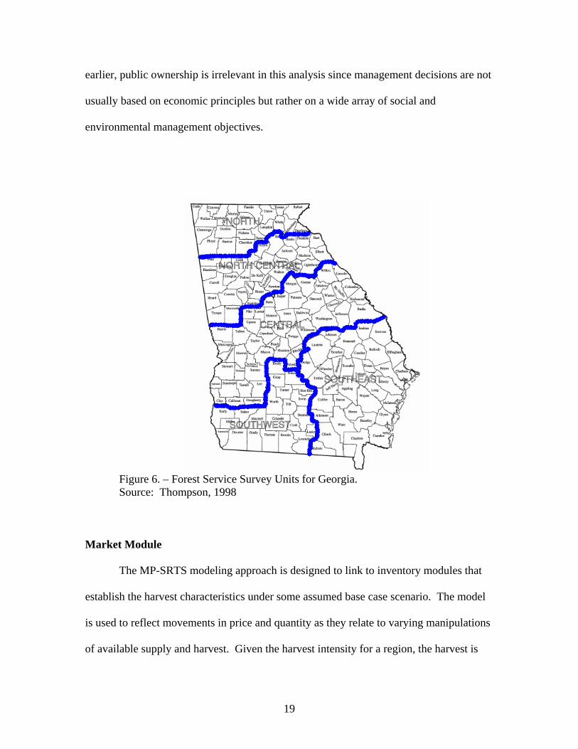
earlier, public ownership is irrelevant in this analysis since management decisions are not

usually based on economic principles but rather on a wide array of social and

environmental management objectives.

Figure 6. – Forest Service Survey Units for Georgia. Source: Thompson, 1998

Market Module

The MP-SRTS modeling approach is designed to link to inventory modules that

establish the harvest characteristics under some assumed base case scenario. The model

is used to reflect movements in price and quantity as they relate to varying manipulations

of available supply and harvest. Given the harvest intensity for a region, the harvest is

19

distributed among the more specific subregional units and the inherent demand, price,

and subregional harvest shifts are calculated. Figure 7 depicts the MP-SRTS market

module and the relative positioning of the inventory module.

DemandPrice orHarvestProjection

by Product

DemandElasticities

by Product

SupplyPrice andInventoryElasticities

by Productby Owner

InventoryShifts

by Product-Owner-Unit

Equilibrium

Price byProduct

Harvest byProduct-Owner-Unit

Goal Program

Inventory Module

Multi-Product Equilibrium

Figure 7. MP-SRTS Market Module

The MP-SRTS algorithm determines the annual harvest based on the quantity

supplied and demanded for each year during the projection period. The harvest level is

assigned at the aggregate region level. For this analysis the aggregate region is the State

of Georgia. Timber supply is a function of several factors with the largest influences

being made by the product prices and inventory levels for the given year. The demand of

raw forest products is a function primarily of price levels at that given time and an array

20

of other influencing factors including: input prices, technological change, land quality,

management, and landowner characteristics. Harvest levels for a given year are based on

the raw forest product prices, initial annual inventory levels, and other supply and

demand shifting variables including management and landowner characteristics. As

harvest levels increase they are assumed to produce a marginal cost per unit. This

implies that the harvest supply function is positively sloping. The initial annual inventory

of merchantable raw forest products positively influences t year’s harvest with constant

elasticity.

In MP-SRTS, modeled inventory changes are used to compute the price, demand,

and supply shifts when the harvest level is assigned to the projection as an exogenous

variable (the most common method used to produce MP-SRTS simulations). The region

is assumed to be at equilibrium at the base year. At this point the demand and supply

variables are known and are used to solve for the price levels of raw forest products and

the inherent demand shift. On the subregional level, the proportion of harvest relative to

the assigned regional harvest level is calculated using the regional price movements and

subregional inventory shifts. The subregional harvest quantities are then adjusted in

order to sum to the amount of the regional harvest. The need for the adjustment comes

from the application of the Cobb-Douglas functional form, which is not additive. The

model can be run assuming that subregional specifications hold and that the aggregate

price is found by using a binary search algorithm that determines the market-clearing

price by summing the supply response across subregions and owners. In addition to

harvest scenarios, timber demand or price can be assigned as exogenous variables where

the remaining market conditions or equilibrium parameters are solved by the model. For

21

this analysis a top-down approach is used and the technique maintains the aggregate

market relationships.

The primary model assumption is that within the region the market is competitive

with no price discrimination between the two ownership classifications. Both NIPF

owners and forest industry owners alike face the same price trends consistent with

economic theory. MP-SRTS represents subregional market conditions that vary

according to regional price levels. Demand is assumed to move between subregions in

response to price movements and comparative advantages among subregional units. For

the life of the projection period, all owners and regions are exposed to the same general

price trend; however, the levels experienced may be different. Comparative advantages

determine the shifts in harvest among owner classes and subregions.

Inventory Module

The GRITS model forms the basis of inventory projections for MP-SRTS. Figure

8 depicts the layout of the MP-SRTS inventory module and the relative positioning of the

market module. The modified internal inventory model allows inventories to be formed

from USDA Forest Service FIA estimates of timberland characteristics. These estimates

include timber removals, growth and inventory, and timberland area. Timber and

timberland estimates are made by five year age class, species and product (softwood

pulpwood, hardwood sawtimber, etc.). Timberland characteristics include being

associated with one of five management types. These management types are: planted

pine, natural pine, oak-pine, upland hardwood, and bottomland hardwood). FIA data by

ten-year age class, species group, product and forest management type are summarized

for each of Georgia’s five subregions and for the State as a single unit.

22

Figure 8. MP-SRTS Inventory Module

Growth. – MP-SRTS, in order to project growth, uses five-year age classes that are

described by species, product, subregion, owner, and management type. Growth is

estimated by a regression equation where growth is a function of the subregion,

ownership class, age and an allowance for interaction between the ownership class and

age. The growth function is modeled as a cubic age relationship. This cubic age

relationship allows the growth to be modeled for the entire state but allows the quantity to

vary by subregion and ownership class.

Harvest. – The approach to harvest allocation within MP-SRTS initiates with distributing

the regional aggregate harvest quantities among the subregions by ownership. The

harvests are distributed based on subregional supply shifts and is part of market

23

equilibrium calculations. On the subregional/owner level, exogenous parameters

allocate harvests by management type and ten-year age class and allow harvests to reflect

historical trends, inventory levels, growth or any weighted combination of these. Timber

harvesting can be distributed by age class within the management type through

proportions of total subregional/owner harvest. For example, higher proportions being

assigned to the older age classifications accomplish an older first approach. Similarly,

assigning the same proportion evenly across age classes allows harvests to be distributed

evenly across all age classes. Abt and others (2000) found through empirical

examination of harvest allocations in the FIA data that for all management types other

than pine plantations, harvest allocations across age classes are highly correlated with

inventory age class distributions.

Model Scenario

The MP-SRTS model can be applied to timber markets at various levels of

resolution for the private forest sector. For the purpose of this analysis the State of

Georgia was considered as a whole and at the FIA survey unit level. The raw timber

product base was established using the 1997 FIA survey, which represents the most

recently completed survey for the area. The simulation is dictated by a depressed level of

growth in demand for raw forest products, which reflects the current timber markets

across the State.

Establishing a base inventory using the FIA data, harvests were allocated for

softwoods by proportions based on management type at a rate of 70% inventory and 30%

growth. This allocation assigns removals to originate from the initial years inventory and

the annual growth proportionately. The softwood harvests were assigned to age classes

24

based on inventory levels for 70% and by an oldest first approach for 30%. Harvest

allocations for hardwood were not assigned based on growth or age class but purely by

the inventory distribution. The harvest levels were adjusted down by 17% in the initial

year (1997-1998) of the projection in order to better reflect realized harvest levels.

The simulation spans from the base year of 1997 to 2025 to encompass a twenty-

eight year projection life. The course of the projection was determined by an annual

growth in the demand for raw forest products at an assigned rate of .5% annually. This

level of demand growth is less than that of previous analysis using SRTS by Abt and

others, 2000, which was assigned at 1.6% based on previous FIA trends. This lower level

of demand growth better reflects the current market for raw forest products for the State

of Georgia.

An increasingly influential factor in the availability of raw forest products in

Georgia is the productivity of pine plantations. Due to variations in management

intensity and development, growth rates are assigned separately to NIPF and industry

ownership classes. Over the life of the projection period, plantations under industry

ownership are assumed to realize a 30% increase in plantation growth rates while a 15%

increase in plantation growth rates for NIPF owners. The growth rate increases are

applied so that the majority is realized in the first half of the projection period and is

assumed to impact all age classes. In addition to the growth rates increasing over the life

of the projection period, the growth rates were increased by 10% initially to reflect

current plantation growth rates.

The timberland base is ever changing as real estate is converted to and from forest

applications. Fluctuations in land use impact the contribution of an area to the timber

25

market and are influenced by factors such as population growth, aggregate U.S. economic

growth, and agricultural and residential land rents. Within the model, movement in land

use is determined based on the regional raw timber product prices. The elasticity of land

use conversion to raw timber product price is assumed to be approximately .3 based on

the findings of Hardie and others (2000). Timber management has aided in the

conversion of natural and mixed pine management types to pine plantations. For the life

of the projection, acres of timberland in pine plantation were held constant at

approximately 26% of the privately held timberland area. Acres under natural and mixed

pine were converted to pine plantation to retain the 26% pine plantation based on the

relative abundance of each within the survey unit. The allowance for conversion among

management types allows the amount of total timberland across the life of the projection

to remain constant.

26

Chapter 3

Results

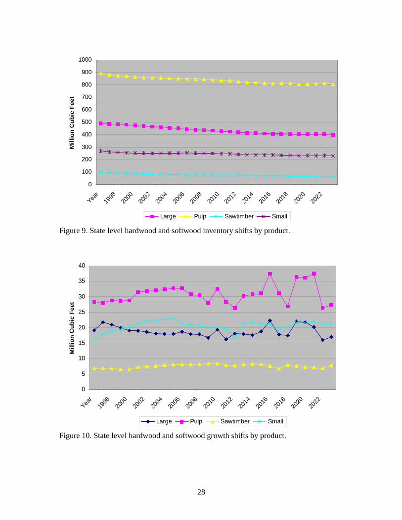
Figure 9 presents the statewide inventory results. Inventories are seen to decline

throughout the projection period with the largest reductions being in pulpwood and large

sawtimber. The growth that is supported from these inventories and influenced by

subregion, ownership class and age is presented in Figure 10. The growth is distributed

around a general flat trend by product; however, the variation in annual growth increases

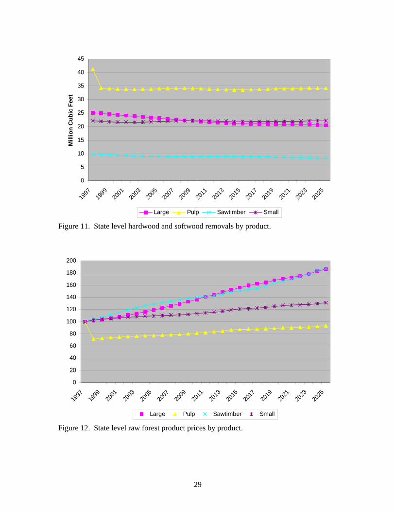
over the projection life. The removals for the State are presented in Figure 11 and remain

unresponsive with the largest shift being in large sawtimber, which declined 16% over

the period. The initial drop in pulpwood removals is a result of pulpwood harvest levels

being adjusted by the administrator prior to performing the simulation. From the 1998

initial harvest level, the projection of pulpwood removals is more closely aligned with

current trends.

The timber product prices are measured in real terms and are presented in Figure

12. The trends are formed using a price index where the price of raw forest products

during the initial year serves as the base and the movement in price is presented as a

percent increase or decrease from the original value. The raw timber product prices

strengthen for the life of the projection period. Sawtimber and large sawtimber

experience the largest increases in product value with approximate increases of 90%.

27

0

100

200

300

400

500

600

700

800

900

1000

Year

1998

2000

2002

2004

2006

2008

2010

2012

2014

2016

2018

2020

2022

Mill

ion

Cub

ic F

eet

Large Pulp Sawtimber Small

Figure 9. State level hardwood and softwood inventory shifts by product.

0

5

10

15

20

25

30

35

40

Year

1998

2000

2002

2004

2006

2008

2010

2012

2014

2016

2018

2020

2022

Mill

ion

Cub

ic F

eet


Figure 10. State level hardwood and softwood growth shifts by product.

28

0

5

10

15

20

25

30

35

40

45

1997

1999

2001

2003

2005

2007

2009

2011

2013

2015

2017

2019

2021

2023

2025

Mill

ion

Cub

ic F

eet


Figure 11. State level hardwood and softwood removals by product.

0

20

40

60

80

100

120

140

160

180

200

1997

1999

2001

2003

2005

2007

2009

2011

2013

2015

2017

2019

2021

2023

2025


Figure 12. State level raw forest product prices by product.

29

The MP-SRTS projections of inventory, growth and removals for softwoods are

presented in Table 1. The projections are categorized by State, FIA survey unit and

product. Data are characterized by product as being pulpwood, small sawtimber,

sawtimber and large sawtimber. The small sawtimber category under softwood products

is commonly referred to as chip-n-saw.

The hardwood data presented in Table 2 is similar to the softwood grouping

however there is no small sawtimber or chip-n-saw category. These projections represent

the potential development of raw forest product inventories throughout Georgia under a

situation of low demand. These forecasts pertain only to timberland holdings under

private ownership and do not consider the implications of publicly owned timberland.

30

Table 1. MP-SRTS Model Softwood Projections by Region 1997 2004 2011 2018 2025

StateInventory Pulpwood 250,928 229,477 216,855 206,503 202,542

Small Saw 213,215 196,753 194,009 183,079 177,520 Sawtimber 99,226 81,516 75,430 69,728 61,012 Large Saw 189,659 150,103 114,678 95,273 83,421

Growth Pulpwood 16,219 19,507 15,960 20,338 18,311 Small Saw 14,641 21,065 18,573 18,274 20,242 Sawtimber 6,799 7,619 8,415 6,762 7,800 Large Saw 12,309 9,605 9,919 10,844 10,806

Removals Pulpwood 23,926 19,702 19,627 19,575 19,847 Small Saw 20,747 20,344 20,652 20,514 20,714 Sawtimber 9,712 8,994 8,863 8,770 8,319 Large Saw 17,378 15,450 13,730 12,965 12,456

NorthInventory Pulpwood 26,306 23,875 22,415 21,201 18,968


Growth Pulpwood 780 890 939 998 589 Small Saw 761 992 1,311 696 904 Sawtimber 117 595 413 583 565 Large Saw 726 507 709 660 887

Removals Pulpwood 1,353 1,095 1,109 1,114 1,084 Small Saw 1,359 1,316 1,337 1,333 1,246 Sawtimber 533 504 508 496 509 Large Saw 1,018 963 938 898 881

NorthcentralInventory Pulpwood 43,897 32,096 21,122 16,749 14,146


Growth Pulpwood 1,920 1,345 1,209 2,119 1,878 Small Saw 1,599 1,705 1,416 2,246 1,976 Sawtimber 1,026 804 873 1,021 1,112 Large Saw 1,946 1,126 1,579 1,670 1,896


- - Thousand Cubic Feet - -

31

Table 1. MP-SRTS Model Softwood Projections by Region (conti…) 1997 2004 2011 2018 2025



Growth Pulpwood 5,547 6,083 5,349 6,785 6,226 Small Saw 5,189 7,115 6,024 5,909 6,372 Sawtimber 2,221 2,613 3,329 3,204 2,799 Large Saw 3,356 2,867 4,139 4,988 5,202


SoutheastInventory Pulpwood 29,093 26,834 27,131 27,067 27,557


Growth Pulpwood 1,799 2,648 1,826 2,432 2,356 Small Saw 1,188 2,687 2,314 2,167 2,368 Sawtimber 729 774 877 980 1,054 Large Saw 2,184 1,482 1,389 2,170 2,271


SouthwestInventory Pulpwood 29,093 26,754 26,882 26,188 26,222


Growth Pulpwood 1,799 2,626 1,811 2,291 2,286 Small Saw 1,188 2,671 2,314 2,098 2,309 Sawtimber 729 760 885 915 1,046 Large Saw 2,184 1,427 1,341 1,882 2,167



32

Table 2. MP-SRTS Hardwood Model Projections by Region 1997 2004 2011 2018 2025


Sawtimber 55,146 54,078 53,236 52,402 51,207 Large Saw 301,720 309,217 311,782 312,476 310,355

Growth Pulpwood 12,096 12,551 16,567 10,772 9,065 Sawtimber 1,099 1,250 1,646 1,172 1,015 Large Saw 6,778 8,434 9,430 6,903 6,176

Removals Pulpwood 17,270 14,221 14,291 14,346 14,348 Sawtimber 1,456 1,447 1,448 1,454 1,452 Large Saw 7,722 7,862 7,942 8,018 8,054

NorthInventory Pulpwood 108,204 110,268 111,449 111,893 114,193


Growth Pulpwood 1,292 856 1,563 1,356 603 Sawtimber 169 61 154 150 75 Large Saw 798 970 1,051 776 441

Removals Pulpwood 944 799 816 834 856 Sawtimber 83 85 87 88 91 Large Saw 411 428 441 452 465

NorthcentralInventory Pulpwood 151,492 156,660 161,842 153,932 140,661


Growth Pulpwood 4,095 3,986 2,369 835 892 Sawtimber 332 422 266 112 127 Large Saw 2,238 2,783 1,508 946 1,067

Removals Pulpwood 3,342 2,821 2,892 2,861 2,774 Sawtimber 294 300 306 305 296 Large Saw 1,480 1,540 1,602 1,611 1,576

CentralInventory Pulpwood 189,439 193,339 200,928 208,701 207,810


Growth Pulpwood 6,362 6,386 7,486 6,769 5,511 Sawtimber 548 681 737 729 612 Large Saw 3,090 4,124 4,307 4,166 3,825

Removals Pulpwood 6,802 5,793 5,982 6,199 6,304 Sawtimber 607 626 645 667 682 Large Saw 3,084 3,208 3,340 3,489 3,575


33

Table 2. MP-SRTS Model Hardwood Projections by Region (conti…) 1997 2004 2011 2018 2025



Growth Pulpwood 1,749 1,905 2,031 1,541 1,673 Sawtimber 162 182 204 182 195 Large Saw 870 1,107 1,291 889 1,074

Removals Pulpwood 1,576 1,340 1,385 1,424 1,452 Sawtimber 140 145 149 154 157 Large Saw 684 716 751 777 798

SouthwestInventory Pulpwood 65,287 64,857 68,027 68,380 67,498


Growth Pulpwood 1,749 1,146 1,890 637 1,507 Sawtimber 162 125 188 101 167 Large Saw 870 801 1,202 465 997

Removals Pulpwood 1,576 1,317 1,355 1,377 1,390 Sawtimber 140 143 146 148 150 Large Saw 684 703 735 752 767


Figure 13 documents the softwood inventory levels across the projection period

by FIA survey unit. The Central FIA survey unit contains the majority of the State’s raw

forest products, particularly pulpwood and small sawtimber. The inventory in the Central

region is relatively unchanged throughout the period with the exception of the large

sawtimber. The North Central region experiences the largest amount of inventory loss

across all product classes due to land conversion. Similarly, Figure 14 documents the

hardwood inventory shifts by product and survey unit. Hardwood inventories remain

unchanged or are seen to increase for the life of the projection period in all regions with

the exception of the North Central region.

34

-

10

20

30

40

50

60

70

80

pulp

woo

d

smal

lsaw

saw

timbe

r

larg

esaw

pulp

woo

d

smal

lsaw

saw

timbe

r

larg

esaw

pulp

woo

d

smal

lsaw

saw

timbe

r

larg

esaw

pulp

woo

d

smal

lsaw

saw

timbe

r

larg

esaw

pulp

woo

d

smal

lsaw

saw

timbe

r

larg

esaw

North Northcentral Central Southeast Southwest

mill

ion

cubi

c ft.

1997 2004 2011 2018 2025

Figure 13. Softwood inventory shifts by FIA survey unit

-

50

100

150

200

250

pulp

woo

d

saw

timbe

r

larg

esaw

pulp

woo

d

saw

timbe

r

larg

esaw

pulp

woo

d

saw

timbe

r

larg

esaw

pulp

woo

d

saw

timbe

r

larg

esaw

pulp

woo

d

saw

timbe

r

larg

esaw


mill

ion

cubi

c ft.

1997 2004 2011 2018 2025

Figure 14. Hardwood inventory shifts by FIA survey unit

35

Figure 15 documents the amount of growth experienced by survey unit and

product class for softwood. Much of the growth is concentrated in the Central region,

which corresponds to the proportion of inventory that the region holds. In most cases the

level of growth is increasing over the projection period as would be expected from the

assigned rates of growth increase in pine plantations. Figure 16 documents the hardwood

growth during the projection period. Unlike softwood trends, hardwood growth over the

projection is forecasted to decline. The most dramatic movements in the level of growth

over the projection period occur in pulpwood, which decreases in four of the five survey

units.

0.00

1.00

2.00

3.00

4.00

5.00

6.00

7.00

8.00

pulp

woo

d

smal

lsaw

saw

timbe

r

larg

esaw

pulp

woo

d

smal

lsaw

saw

timbe

r

larg

esaw

pulp

woo

d

smal

lsaw

saw

timbe

r

larg

esaw

pulp

woo

d

smal

lsaw

saw

timbe

r

larg

esaw

pulp

woo

d

smal

lsaw

saw

timbe

r

larg

esaw


mill

ion

cubi

c ft.

1997 2004 2011 2018 2024

Figure 15. Softwood growth shifts by FIA survey unit

36

0.00

1.00

2.00

3.00

4.00

5.00

6.00

7.00

8.00

pulp

woo

d

saw

timbe

r

larg

esaw

pulp

woo

d

saw

timbe

r

larg

esaw

pulp

woo

d

saw

timbe

r

larg

esaw

pulp

woo

d

saw

timbe

r

larg

esaw

pulp

woo

d

saw

timbe

r

larg

esaw


mill

ion

cubi

c ft.

1997 2004 2011 2018 2024

Figure 16. Hardwood growth shifts by FIA survey unit The inventory coupled with the annual growth can depict trends that present how

and in which regions the timber resources in Georgia are plentiful. With Figures 17 and

18 the amount of pressure that is being placed on these inventories is evident. These

expected timber harvest trends document where opportunities exist for increased use of

raw forest products. Figure 17 presents the softwood harvest levels for the projection

period by FIA survey unit. In most cases the harvest levels remain relatively unchanged.

The North Central survey unit, unlike the other regions, experiences sharp declines in

harvest levels for all product classes. In Figure 18 the hardwood harvest levels are

presented. These levels remain constant for all regions except for the Central survey unit

which experiences increasing levels of harvest over the projection interval.

37

0.00

1.00

2.00

3.00

4.00

5.00

6.00

7.00

8.00

pulp

woo

d

smal

lsaw

saw

timbe

r

larg

esaw

pulp

woo

d

smal

lsaw

saw

timbe

r

larg

esaw

pulp

woo

d

smal

lsaw

saw

timbe

r

larg

esaw

pulp

woo

d

smal

lsaw

saw

timbe

r

larg

esaw

pulp

woo

d

smal

lsaw

saw

timbe

r

larg

esaw


mill

ion

cubi

c ft.

1997 2004 2011 2018 2025

Figure 17. Softwood removals by FIA survey unit

0.00

1.00

2.00

3.00

4.00

5.00

6.00

7.00

8.00

pulp

woo

d

saw

timbe

r

larg

esaw

pulp

woo

d

saw

timbe

r

larg

esaw

pulp

woo

d

saw

timbe

r

larg

esaw

pulp

woo

d

saw

timbe

r

larg

esaw

pulp

woo

d

saw

timbe

r

larg

esaw


mill

ion

cubi

c ft.

1997 2004 2011 2018 2025

Figure 18. Hardwood removals by FIA survey unit

38

The implication of movements in inventory and growth, and the pressure that is

applied to the inventories through harvest is the resulting price of raw forest products.

Product prices dictate much of the activity that takes place within the industry and impact

the strategic planning of many entities within the forest sector. By exploring the

projected price levels, movements within the industry can be identified and possibly

addressed through governmental policy. Price forecasting in this fashion allows users of

the forest resources to better plan and invest capital efficiently. The administrator prior

to performing the simulation adjusted the pulpwood projections in this analysis. The

initial drop in year one (1997-1998) represents a realized reduction in harvest levels of

17%. The manipulation allows projections to reflect harvest levels that have been

realized thus far in the projection period.

Figure 19 presents the projected price levels for forest products for the Northern

survey unit. The pulpwood price level has been adjusted in year one as explained earlier.

The price of sawtimber peaks in 2002 and begins to decline till the end of the period.

Pulpwood and small sawtimber prices increase for the entire period while large

sawtimber prices increase most noticeably during the first half of the projection period.

Figure 20 documents the raw timber product price projection for the North

Central region, which are all increasing for the life of the projection. Figure 21

represents the price projections for the Central region. This area as presented previously

has the largest amount of inventory in the State and the product prices within the region

remain relatively unchanged over the projection period.

In Figure 22, the price projections pertain to the Southeastern survey unit. The

product price for sawtimber and large sawtimber increase rapidly until 2015 when they

39

both decelerate and gradually continue to increase toward the end of the period. Small

sawtimber and pulpwood products remain relatively unchanged over the period. The

Southwestern region experiences similar price movements over the period with

sawtimber and large sawtimber increasing in real terms.

0

20

40

60

80

100

120

140

1997

1999

2001

2003

2005

2007

2009

2011

2013

2015

2017

2019

2021

2023

2025


Figure 19. Raw timber product price projections for the Northern survey unit.

40

0

50

100

150

200

250

300

350

1997

1999

2001

2003

2005

2007

2009

2011

2013

2015

2017

2019

2021

2023

2025


Figure 20. Raw timber product price projections for the North Central survey unit.

0

20

40

60

80

100

120

140

1997

1999

2001

2003

2005

2007

2009

2011

2013

2015

2017

2019

2021

2023

2025


Figure 21. Raw timber product price projections for the Central survey unit.

41

0

20

40

60

80

100

120

140

160

180

1997

1999

2001

2003

2005

2007

2009

2011

2013

2015

2017

2019

2021

2023

2025


Figure 22. Raw timber product price projections for the Southeastern survey unit.

0

20

40

60

80

100

120

140

160

180

200

1997

1999

2001

2003

2005

2007

2009

2011

2013

2015

2017

2019

2021

2023

2025


Figure 23. Raw timber product price projections for the Southwestern survey unit.

42

Chapter 4

Conclusions

The MP-SRTS model is a strategic planning tool with the capabilities of

identifying opportunities for expansion/contraction within the forest sector and possible

needs for protection from or encouragement for modified forest policy. The model has

evolved from previous approaches to better project the forest market conditions of more

specific areas, which has increased the model’s applications and benefits. The MP-SRTS

model allows inventory conditions to be given an economic overlay that is capable of

forecasting future conditions by specific area and product class and has allowed

information to be tailored for individual entities within the forest sector.

This analysis has examined the response of the Georgia regional and subregional

markets to the conditions aligned with a lower demand scenario for raw forest products.

The low demand scenario still results in a statewide decline in raw forest product

inventories which gives rise to increased prices over the period of the projection for most

products. The harvest levels are predicted to remain level for the projection period.

Regional responses vary among survey units and between species class, from

drastic reductions in softwood inventory as seen in the North Central region to increasing

hardwood inventories such as in the Central region. Fluctuations are predicted to be

more drastic in softwood inventories with hardwood levels remaining relatively constant

if not increasing. The Central survey unit contains the largest amount of timber resources

within the State. This region is predicted to supply the largest amount of raw forest

43

products to the forest industry by sustaining the largest projected harvest. Hardwood and

softwood harvests are expected to return to 1997 harvest levels by the end of the

projection period.

As the inventory, growth, and harvest levels vary the price levels fluctuate widely

among the five survey units and may indicate operational opportunities. The North

Central region experiences dramatic price increases over the period of the projection and

is influenced by the growing metropolis, Atlanta. In most cases the price projected for

raw forest products increases over the projection period. This is an expected outcome in

that the inventory declines and harvests are relatively constant which applies upward

pressure on the price of raw forest products.

There are several weaknesses in the MP-SRTS approach. Projecting future

market conditions using MP-SRTS assumes that historical trends hold true, which may

not be the case in some areas, particularly those with high levels of urbanization.

Projecting inventory levels using product specifications generates issues in that stands are

assumed to contain a historically consistent distribution of products when being “grown”

in the inventory model. As management techniques are implemented, such as thinning

treatments, stands will undoubtedly be changed to support a larger amount of higher end

products. This shift from previous product distributions to being proportionally skewed

toward sawtimber is not fully reflected in the inventory component of the MP-SRTS

model. The MP-SRTS model however is a useful tool and can be adapted to address

future needs of the forest sector. The use of MP-SRTS provides entities within the forest

sector with a tool for management and long term planning.

44

References

Abt, R., F. Cubbage, and G. Pacheco. 2000. Southern forest resources assessment using

the Sub-Regional Timber Supply (SRTS) model. Forest Products Journal. 50(4):

25-33.

Barlow, S.A., I.A. Munn, D. A. Cleaves, and D.L. Evans. 1998. The effect of urban

sprawl on timber. Journal of Forestry. 96(12): 10-14.

Birch, T.W. 1996a. Private forestland owners of the United States, 1994. Res. Bull. NE-

134. USDA Forest Service, Northeastern For. Exper. Station, Radnor, PA. 183 p.

Birch, T.W. 1996b. Private forestland owners of the Southern United States, 1994. Res.

Bull. NE-138. USDA Forest Service, Northeastern For. Exper. Station, Radnor,

PA. 195

Clutter, Mike L., B. Mendell, D. Newman, D. Wear, J. Gries. 2005. Strategic Factors

Driving Timberland Ownership Changes in the U.S. South. USFS Working Paper.

2005.

Cost, N. D. 1989. Multi-resource inventories in the southeast. USDA For. Ser. Res. Pap.

SE-269.

Cubbage, F.W., D.W. Hogg, T.G. Harris and R.J. Alig. 1990. Inventory projection with

the Georgia Regional Timber Supply (GRITS) Model. Southern J. of Appl.

Forestry 14(3): 137-142.

Cubbage, Frederick W., Jacek P. Siry, and Robert C. Abt. 2006. Fast Grown Plantations,

Forest Certification, and the U.S. South: Environmental Benefits and Economic

45

Sustainability. Prepared for Submission to the New Zealand Journal of Forest

Science.

DeCoster, L.A. 1998. The boom in forest owners-A bust for forestry? Journal of Forestry

96(5): 25-28.

Hardie, Ian. Peter Parks, Peter Gottleib, and David Wear. 2000. Responsiveness of rural

and urban land uses to land rent determinates in the U.S. South. Land Economics.

76 (4); 659-673.

Haynes, R.W. 1990. An analysis of the timber situation in the United States: 1989-2040.

For. Resour. Rpt. 23. Washington, DC. USDA Forest Service. 499 p.

Haynes, R.W., 2003. An analysis of the timber situation in the United States: 1952 –

2050. General Technical Report. Portland, OR: USDA Forest Service, Pacific

Northwest Research Station.

Johnson, T.G., J.L. Wells. 2005. Georgia’s timber industry – an assessment of timber

product output and use, 2003. Resour. Bull. SRS-68. Asheville, NC: U.S.

Department of Agriculture Forest Service, Southern Research Station.

Mehmood, S.R. and D.W. Zhang. 2001. Forest parcelization in the United States – A

study of contributing factors. Journal of Forestry. 99(4): 30-34.

Mills, J.R. and J.C Kincaid. 1992. The Aggregate Timberland Assessment System-

ATLAS: A comprehensive timber projection model. Gen. Tech. Rept. PNW-

GTR-281. USDA Forest Serv., Pacific Northwest Res. Sta., Portland, OR.

Nagubadi, R.V. and D. Zhang. 2004. Determinants of timberland use by ownership and

forest type in Alabama and Georgia. Journal of Agricultural and Applied

Economics, 37,1 (April 2005): 173-186.

46

Prestemon, Jeffrey and Robert Abt. 2003. Timber products supply and demand. P. 299-

326. In: Wear, D.N., and J.G. Greis, Editors, Southern Forest resource

Assessment. General Technical Report SRS-53. USDA Forest Service, Southern

Research Station. Asheville, North Carolina, USA.

Riall, B. W., 2002. Economic Benefits of the Forestry Industry in Georgia: 2001.

Research Services, Economic Development Institute, Georgia Institute of

Technology. 21 pp.

Siry, Jacek P., Frederick W. Cubbage, David H. Newman. 2005. Who Owns the World’s

Forests? Implications for Forest Production, Management, and Protection. 2005

IUFRO World Congress proceedings. Paper Prepared for Submission to Forest

Policy and Economics. In Press.

Smith, W. Brad, Patrick D. Miles, John S. Vissage, and Scott A. Pugh. 2004. Forest

Resources of the United States, 2002. General Technical report NC-241. St.

Paul, MN: USDA Forest Service North Central Forest Experiment Station. 137 p.

Thompson, Michael T. 1998. Forest Statistics for Central Georgia, 1997. Resour. Bull.

SRS-26. Asheville, NC: U.S. Department of Agriculture, Forest Service, Southern

Research Station. 60 pp.

Timber Mart-South, 2006. Personal Communication.

U.S. Department of Agriculture Forest Service. 2006. Forest Inventory and Analysis

database. February 13-15, 2006.

Wahlenberg, W.G. 1960. Loblolly Pine. Duke University School of Forestry, Durham,

N.C. 603 p.

47

assessing the timber situation in georgia using the …

Documents