Assessing the synergistic effect of two invasive

plants on native plant communities in Kanha

National Park, Central India

Dissertation submitted to Saurashtra University, Rajkot

In partial fulfilment of

Master’s degree in Wildlife Science

2015-2017

By

Rajat Rastogi

Under the supervision of

Shri Aseem Shrivastav

Prof. Qamar Qureshi

Dr. Y. V. Jhala

Assessing the synergistic effect of two invasive plants on native plant

communities in Kanha National Park, Central India

ACKNOWLEDGEMENT

This journey from being undergraduate student in Zoology to a master’s (almost) in Wildlife

Science was full of thrill, excitement, twists and turns. The Wildlife Institute of India (WII) has

been a major growth factor for me both in my personal life and professional life and I will

always be indebted to it. Taking this opportunity firstly, I thank Director, Dean, all faculties and

staff members at WII for their support and guidance at each and every step in these two years.

My sincere gratitude goes to my supervisors, Shri Assem Shrivastav, Prof Qamar Qureshi

and Dr Y.V. Jhala. Their support in completion of this study has been immense and I consider

myself lucky to have you as my source of guidance.

I am hugely grateful to PCCF, CWLW Madhya Pradesh and Sanjay Shukla sir (Field

director), K.S. Bhadauria sir (Joint Director), Anjana Suchitra Tirki mam (Deputy director-

Buffer), Rakesh Shukla sir (Research officer), Sandeep Agarwal sir (Veterinarian) Kanha

Tiger Reserve to provide permissions to live in the sacred scape of Kanha and study biological

invasions. I thank Sudhir Mishra sir and Surendra Kumar Khare sir (Assistant Directors, Kanha

NP), Uttam Singh ji (Range Officer, Mukki range), Kranti Jhariya ji (RO, Sarhi Range and

Kanha Range), Pathak ji (RO, Kisli range) and Narpat Singh Markam ji (Asst. RO, mukki

range) for creating a healthy and supportive environment and I thank them for all the support

and guidance. I thank the extremely hard working and enthusiastic field staff at Kanha it has

been a journey of immense learning and exploration with them. Their warm and caring nature

made it so difficult for me to return back to the headquarters at Dehradun.

I now extend my gracious gratitude and regards to ‘& Beyond-Taj Safari (Banjaar tola, Kanha

NP)’ for being my external funding agency and providing monetary support for the study, it

would have been really tough for me to successfully complete this study without your support. I

am especially grateful to Ms Mridula Tangirala, Mr Amit Kumar, Mr Narayan Rangaswami and

other friends at Banjaar tola, for their help and support. Thanks a lot.

I would like to thank Prem Sir, Padma mam and other staff from the academic cell to keep us as

their own kids, during these two years. I thank Mr Harikrishan and Mr Madan lal, Accounts

section, for their speedy release of funds during our study tours and during dissertation. I thank

Vinod Thakur sir, Ajay Sharma sir and Rakesh Sundriyal sir, Anita Devi, Monika Sharma and

Ajay Shrivastav for their support in lab analysis.

I now thank Ms Shivani Shrivastava, Mr Nishant Kumar (XIII M.Sc. WII), Ms Neha Awasthi

and Naman Goyal, who have nurtured the wild seed inside me and have shown me the path, on

which I walk today. I thank all my school teachers at Bal Bharti Public School, Mawana and

Translam Academy International, Meerut, to ingrain curiosity in my mind and help me grow

with it. I thank my professors at Deshbandhu College, University of Delhi to set me free and let

me fly like Black Kite (Milvus migrans) in and around the corners of our country to learn and

explore.

I thank my flatmates and friends, Shruti, Himanshu, Kaku, Abhinav, Mrinal, Harsha, Shubh,

Deepu, Vikas, Neha, Divya, Anu, Dev and Mayank (soulmates precisely ^.^) to harass and love

me like anything. I am thankful to Visha for supporting me in the hard times and being a shield.

I thank Ankita Sahrawat and Aishwarya Bhandari for their kind support during my undergrad

and grad life. I thank the XV M.Sc. for being the devil and diva, handling with love and care,

this cranky mind all through these two years. It was because of you guys that, classes were fun

and field was life. Samyuktha, being the most sincere late comer and Ashish being the silent

soul, Ravi’s lephad talk and Ankit (Golu) being our Elephus. I enjoyed the subtle company of

Monisha (momo) and ever jumping priyanka (Justa nivas). Nimisha and sultan giving the UP

wala feel and Krishna’s wonly in every presentation. Rakesh’s simplistic yet bong attitude,

Rohi’s sketching and Ashwin’s political corrections, Naman and Aishwarya comes with no

mention, since, they were already a part of this journey since our Kite days. I will miss these

days throughout my life. I thank you all for being there.

I thank Ms Jade Bernard, a beautiful soul from Salt Spring Island for giving me a good friend

for life. Deep thanks to Ms. Rutu Prajapati, Mr Deb Ranjan Laha and Mr Anup Pradhan for

teaching me about the field techniques and being an integral part of my life. I also thank Mr

Jayanata borah, Ms Shravana Goswami and Mr Sanjay Xaxa for being a nice company in

Kanha. I thank Ms Madhura Davate, Ms Ridhima Solanki, Mr Neeraj Mahar, Ms Ankita

Bhattacharya, Ms Dimpi Patel, Dr Vishnupriya Kolipakam, Dr Bopanna Ponappa, Ms Shikha

Bisht, Mr Anant Pande, Ms Ankita Sinha, Mr Bipin C.M., Ms Amrita Laha, Ms Pritha Dey, Ms

Preeti Virkar, Preeti, Keshab, Deepak, Harsh, Bheem, Moumita, Oyndrilla, Adrita and all other

people whom I am forgetting right now. I deeply enjoyed the time spent with all of you.

I am grateful to Ninad, Dr Monika Kaushik, Dr Kavita Iswaran, Dr Suhel Quader, Dr Adwait

Edgaonkar and endless people who have helped me in conceptualizing and designing the current

study. I am thankful to my extended field family Manish, Manjhla, Satish, Kanhaiya, Nirottam,

Kamlesh ji, Abir and Chintu bhaiya for helping me out and being there for me, whenever I

needed. I thank Mr Ujjwal Kumar for being big brother and Dr Sutirtha dutta and Dr Rashid

Raza for brainstorming during the analysis season during the six month dissertation.

I whole heartedly thank Bivash Sir, Rawat Sir, Qamar sir and Gopi sir, for the much needed

moral boost up during the last two semesters.

I extend my warm regards to IRCH, and AIIMS, New Delhi, for their speedy actions.

Completing this thesis and preparing defence presentation in the corridors, staircase and on the

roads has been an experience on its own. I thank Dr Lalit Kumar and his full team for taking

care of my loved ones. I thank Ankita Dhondiyal, Dietician at IRCH, AIIMS, for being a pillar

of positivity during the time we were at AIIMS. I am thankful to Nitish Kumar, Dr Priyankar

dutta, Abhilash Prabhat, Kashish, Anu mam, Vishal, Kartik, Harru, for reasons best known to all

of us.

I thank my invaders Lantana camara and Pogostemon benghalensis, without whom this study

could have never been thought about and of course, bububabam :P, for holding it all together

despite all odds.

I thank readers for taking so much pain, to go through this document and I also apologize for the

flaws and mistakes, I have done in the write-up.

All this is one part of the story, but nothing will ever be complete, without the support of my

family. My deepest love and thanks to mumma, papa, amma, bhai, gudda and other family

members for their support all through this journey. It is because of the freedom provided by

them that I could deliver this work to all of you.

- Rajat Rastogi

Table of Contents

Chapter

number Chapter title

Page

number

Acknowledgement

List of Tables

List of Figures

Summary 1

1 Introduction

Background 3

The question 6

2 Methods

Study area & Study design 7

Laboratory methods 12

Statistical analyses 12

3 Results

Distribution of Invasive plants 18

Species composition and community structure 25

Comparing response variables along the

aaaaaaaagradient of plant invasion using linear model

aaaaaaaa(ANOVA) 30

4 Discussion

Distribution of Invasive plants 34

Species composition and community structure 35

Biotic homogenization 37

Invasional meltdown hypothesis 38

Intermediate disturbance hypothesis 39

5 Conclusion 40

References

Appendix S1

Appendix S2

Appendix S3

Appendix S4

Appendix S5

Appendix S6

Appendix S7

Appendix S8

Appendix S9

Appendix S10

List of tables

Table

number Table title

Table 1 Invasion matrix showing thirteen classes of invasion, based on the

percent cover of Lantana and Pogostemon.

Table 2 Physiological parameters, germination success and environmental

stress threshold of lantana and pogostemon in the study area; used for

deriving the mechanistic model of species.

Table 3 Relative contribution of different environmental parameters to explain

the presence or absence of lantana in study area in different correlative

SDMs.

Table 4 Relative contribution of different environmental parameters to explain

the presence or absence of pogostemon in study area in different

correlative SDMs.

Table 5 Comparing the discriminatory power of SDMs for differentiating

species’ presence and absence using the sensitivity index, specificity

index and model performance.

Table 6 Proportion of variations explained by different components of

Canonical Correspondence Analysis (CCA) and their eigen values.

Table 7 Relationship of environmental parameters with different components

of CCA.

Table 8 Mean values of diversity and soil parameters arranged in the categories

of invasion at 10X10m scale.

List of Figures

Figure

number Figure title

Figure 1

Cumulative increase in studies (n=132) reporting invasional

meltdown hypothesis, since 1999 when the hypothesis was

proposed.

Figure 2 Arrangement of 120 sampling plots depicting overall sampling

effort in the increasing magnitude of Lantana and Pogostemon.

Figure 3

Plots surveyed across the Sal forest in the study area to record

the abundance of lantana (red), pogostemon (blue), both

(maroon) and none (green). Inserted map on the top right corner

shows the geographic location of study area in the Kanha

National Park, Madhya Pradesh, India. Inserted figure on

bottom right shows the survey design where transect (A) and

perpendicular to it (B, C) were walked to sample the plots

(black points).

Figure 4 (a) Alignment of sampling plots in a 100X100m grid,

Figure 4 (b) A sampling plot with arrangement of 1X1m sub plots.

Figure 5

Lantana distribution modelled by Linear Model (LM),

Occupancy Model (OM), Maximum Entropy (MaxEnt),

Biophysical Threhold Model (BTM), Biophysical Density

Model (BDM) and Ensemble of all these models (Ensemble) in

the study area

Figure 6

Pogostemon distribution modelled by Linear Model (LM),

Occupancy Model (OM), Maximum Entropy (MaxEnt),

Biophysical Threshold Model (BTM), Biophysical Density

Model (BDM) and Ensemble of all these models (Ensemble) in

the study area.

Figure 7 Species accumulation curve for trees, shrub and herbs.

Figure 8 Stress plot for Non-metric multidimensional scaling (Non

metric fit, R2=0.963).

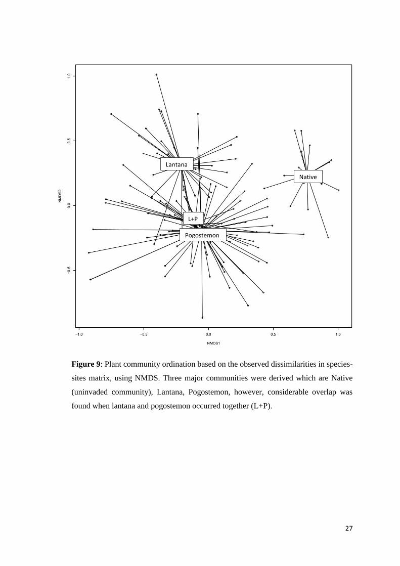
Figure 9 Plant community ordination based on the observed

dissimilarities in species-sites matrix, using NMDS.

Figure 10

Correlation of Native species with abundance of lantana,

pogostemon, environmental parameters and edaphic factors

using Canonical Correspondence Analysis.

Figure 11 Map showing the location of 24 grids (100X100m)

1

SUMMARY

1. Over time, community assembly and functioning of native ecosystems is

known to shift from native species to non-native species thus, restructuring the

native community. When this shift of diverse native ecosystem interaction to

less diverse invasive-centric interaction, occurs due to synergistic effect of two

invasive species, it is known as ‘invasional meltdown’. Since last two decades,

the effects posed by invasive species on ecosystems are widely debated.

Studies across the globe have reported simplification in community structure

with biological invasions, leading towards monotonous ecosystems and

homogenization of biodiversity.

2. I assessed the interaction of two invasive plant species, Lantana camara

complex (lantana) and Pogostemon benghalensis (pogostemon) with native

understorey vegetation in Shorea robusta (Sal) forest of Kanha National Park,

Central India. Here, I tested biotic homogenization, invasional meltdown and

intermediate disturbance hypothesis. To achieve this, 56 km2 out of 230 km

2 of

Sal forest covering 5613 cells (100X100m) was extensively surveyed, to model

species distribution of lantana and pogostemon using different correlative,

mechanistic and ensemble models. From the surveyed area, 120 plots

(10X10m) were selected based on the percent cover of invasive species, where

vegetation and soil sampling was conducted. The correlations in community

composition with edaphic and climatic parameters were established using non-

parametric ordination, and the potential effects of single invasive species and

their interaction were estimated using linear models by considering the

uninvaded plots as control.

3. From the sampled area, 40 km2 (71%) and 37 km

2 (66%) were found to be

invaded by lantana and pogostemon respectively. Lantana presence was best

explained as a function of nearby lantana density and was constrained by

evapo-transpiration rate of summer, light availability and dry stress. Whereas,

pogostemon presence was best explained by moistness of forest patch, lower

summer temperature and habitat openings due to anthropogenic factors and

was constrained due to climatic heat, edaphic dry stress, and remote deciduous

forest.

2

4. I found that the plant species composition differed between uninvaded and

invaded plots. A negative correlation of Shorea robusta was also found when

lantana and pogostemon were present together. Linear Models established a

significant decrease in native plant diversity and richness of rare plants

(5.33±0.10), with an increase in pogostemon (0.67±0.29) and lantana

abundance (0.50±0.38). However, when both invasive species were present, a

substantial decline in native species diversity, richness of rare plants

(0.40±0.36), soil moisture and an increase in species evenness, soil organic

carbon and soil potassium was assessed.

5. Study results indicate an insignificant effect of intermediate disturbances, and

significant impacts of invasive species on species composition and edaphic

factors, thereby affirming the biotic homogenization and invasional meltdown

hypothesis and rejecting intermediate disturbance hypothesis. Present study

can be used as an evidence to prioritize immediate management interventions

in areas where multiple invasions are present, as the chances of extirpation of

rare species is high.

Keywords: Single invasion, multiple invasions, Lantana camara, Pogostemon

benghalensis, invasional meltdown, biotic homogenization, species distribution

models (SDM)

Field view 1: Lantana camara invasion on the banks of a stream bed in Kanha.

3

CHAPTER ONE: INTRODUCTION

Background

In the very first episode of its second season, Planet Earth, one of the most popular

web series showcasing global biodiversity, highlighted the synergistic effects of

multiple species invasions on island ecosystem (BBC media centre, 2016). This

popularity reflects the growing concern on biotic homogenization of the earth due to

“a few winners replacing many losers in the next mass extinction” (McKinney &

Lockwood, 1999); invasive species are one such winner. Invasive species are native or

non-native species with established viable populations, which tends to modify the

native ecosystem in a short span of time (Colautti and MacIsacc 2004, Blackburn et al.

2011). Biotic homogenization (Sax et al, 2005), reduction in biodiversity (Hejda et al.

2009, Shea and Chesson, 2002, Thelen et al., 2005), alteration in nutrient cycling

(Wright et al., 2014, Sharma and Raghuvanshi, 2009) are some of the characteristics

shown by them.

Release from controlling agents (enemy release hypothesis; Keane 2002), high

phenotypic plasticity (Elton, 1958) and genetic diversity (Ray and Quader 2014)

mostly help the invasive species to exploit essential resources. Invasive species alter

the dynamics of invaded ecosystem and the interactions within the biotic and abiotic

components of the invaded area (Green et al., 2011, Martin et al., 2009, Mcgrath &

Binkley, 2009). Being opportunistic, they can sustain in limited amount of resources

and induce changes in the soil chemistry, making it undesirable for native plants. Such

allelochemicals are known to reduce the abundance and richness of native plants, at

times resulting in local extinction. Dassonville et al. 2007 found invasion of Fallopia

japonica (Japanese knotweed) increased top soil mineral contents by enhancing

nutrient recycling rates leading to soil homogenization. Ehrenfeld et al. 2001 attributes

changes in soil chemistry by Berberis thunbergii, a woody shrub, and Microstegium

vimineum, a C4 grass, to decrease in native plant richness following exotic understorey

plant invasion. High magnitude of such changes can restructure the native ecosystem

interactions to invasion centric interactions (Simberloff 2006). This restructuring due

to synergistic effects of two invasive species can further facilitate other invasive

species and magnify the impacts on native ecosystems, a hypothesis proposed as

‘invasional meltdown’ (Simberloff & Van holle 1999).

4

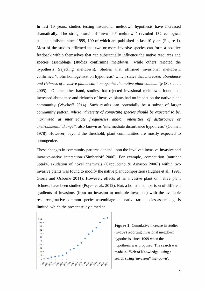
In last 10 years, studies testing invasional meltdown hypothesis have increased

dramatically. The string search of ‘invasion* meltdown’ revealed 132 ecological

studies published since 1999, 100 of which are published in last 10 years (Figure 1).

Most of the studies affirmed that two or more invasive species can form a positive

feedback within themselves that can substantially influence the native resources and

species assemblage (studies confirming meltdown); while others rejected the

hypothesis (rejecting meltdown). Studies that affirmed invasional meltdown,

confirmed ‘biotic homogenisation hypothesis’ which states that increased abundance

and richness of invasive plants can homogenize the native plant community (Sax et al.

2005). On the other hand, studies that rejected invasional meltdown, found that

increased abundance and richness of invasive plants had no impact on the native plant

community (Wyckoff 2014). Such results can potentially be a subset of larger

community pattern, where “diversity of competing species should be expected to be,

maximized at intermediate frequencies and/or intensities of disturbance or

environmental change”, also known as ‘intermediate disturbance hypothesis’ (Connell

1978). However, beyond the threshold, plant communities are mostly expected to

homogenize.

These changes in community patterns depend upon the involved invasive-invasive and

invasive-native interaction (Simberloff 2006). For example, competition (nutrient

uptake, exudation of novel chemicals (Cappuccino & Arnason 2006)) within two

invasive plants was found to modify the native plant composition (Hughes et al,. 1991,

Gioria and Osborne 2011). However, effects of an invasive plant on native plant

richness have been studied (Psyek et al,. 2012). But, a holistic comparison of different

gradients of invasions (from no invasion to multiple invasions) with the available

resources, native common species assemblage and native rare species assemblage is

limited, which the present study aimed at.

Figure 1: Cumulative increase in studies

(n=132) reporting invasional meltdown

hypothesis, since 1999 when the

hypothesis was proposed. The search was

made in ‘Web of Knowledge’ using a

search string ‘invasion* meltdown’.

5

For this, I first estimated the densities of Lantana camara complex (Lantana,

henceafter), an introduced species, and Pogostemon benghalensis (Pogostemon,

henceafter), a native weed, through extensive sampling in the Shorea robusta (Sal,

henceafter) forest of Kanha National Park in Central Indian landscape. I derived

Species Distribution Maps (SDMs) and tested correlative and mechanistic models to

predict their presence and absence. From the surveyed area, 120 plots of 10X10m each

were selected based on the cover of invasive species, to record abundance of native

and invasive plant species. I calculated diversity parameters like species richness,

species evenness and Shannon-Weaver diversity index and assessed plant community

structure and composition using non-metric multidimensional scaling (NMDS) and

Canonical Correspondence Analysis (CCA).

Both species, being opportunistic are expected to extract nutrients from the top soil

level, thereby altering with the soil nutrient composition. With this change in soil

chemistry, native plant richness is expected to decrease with the increasing abundance

of the invasive plants. In the present study, I also tested invasional meltdown

hypothesis (Simberloff and Von Holle 1999), intermediate disturbance hypothesis

(Connell 1978) and biotic homogenisation hypothesis (McKinney and Lockwood,

1999) for invasion of lantana and pogostemon using linear models.

Field view 2: Morning view of open Shorea robusta forest invaded with Lantana

camara and Pogostemon benghalensis.

6

The Question

To test Invasional meltdown hypotheses, Biotic homogenization hypothesis and

Intermediate disturbance hypothesis, the following objectives and research questions

were studied:

Objective 1: To estimate the distribution and density of Lantana camara and

Pogostemon benghalensis in Sal forest of Kanha National Park.

Research question:

1. How are Lantana and Pogostemon distributed in sal forest of study area?

2. Which environmental parameters explain their presence and absence?

Objective 2: To assess the difference in plant species composition along the gradient

of plant invasion.

Research questions:

1. Is there a difference in species composition of invaded and uninvaded areas?

2. What is the relationship between environment and plant community in the

study area?

3. What is the difference in species richness, diversity, evenness of native plants

and edaphic factors across the plant invasion gradient?

Field view 3: Pogostemon benghalensis invasion along the bank of a stream in Kanha.

7

CHAPTER TWO: STUDY AREA AND METHODS

Study area and design

The present study was conducted in Kanha National Park in Madhya Pradesh. Kanha

NP is a part of central Indian highlands and extends from 22o 02’ 52” N to 22

o 25’ 49”

N and 80o 30’ 09” E to 81

o 02’ 49” E. This 940 km

2 broad area has a mosaic of four

major forest type viz. Shorea robusta dominated forest, Shorea - Terminalia

dominated miscellaneous forest, bamboo forest and grasslands. Kanha harbours a wide

range of flagship species and endangered species, some of which are Tiger (Panthera

tigris tigris), Gaur (Bos gaurus), Wild dog (Cuon alpinus), Barasingha (Rucervus

duvaucelli branderi), Vulture (Gyps sp.). Apart from native plants, the area also has

numerous weed species like Senna tora, Lantana camara, Pogostemon benghalensis,

Parthenium hysterophorus, Ageratum conyzoides, Hyptis suaveolens etc. that are

known to affect the habitat of endangered flagship species in the park (Management

plan, 2010).

Taking into consideration, objectives of the study and diverse habitat types of Kanha

NP, Shorea robusta (Sal) dominated forest in the four western ranges (i.e, Kisli,

Kanha, Mukki and Sarhi) was selected to be the intensive study area. Rationale behind

this selection was to minimize the innate variability in plant understorey composition

caused due to heterogeneous forest type. Selected ranges in the study area also share

similarity in weather conditions, moisture regime and management timeline. Although,

the other two ranges, namely, Supkhar and Baisanghat, hold good percentage of Sal

dominated forests but are relatively moister, hilly (undulating), dissimilar in weather

conditions, because of which they were excluded from the current study.

METHODS:

For objective 1: A map of drier Shorea robusta (sal) forest of Kanha National Park

(geographically located in the Kanha, Kisli, Mukki and Sarhi forest ranges of the park)

was obtained from the Management plant (2010). The forest was divided virtually in a

grid of 100X100m using a GIS domain. 1 or 2 non-overlapping straight transects of 2

km (Fig 3A) were walked in the sal forest of every beat (an administrative unit of the

forest department, 15-20 km2) in the study area. At every 100m, a perpendicular

distance of 200 m (Fig 3B) to transect was walked along which five plots of 15m

radius were sampled at every 40 m distance. At these plots another perpendicular

8

distance of 40m (Fig 3C) was walked on both the sides and a plot was sampled. At

each plot, percent cover of all the invasive plants, ocular canopy cover, and number of

native trees were recorded. In addition to this, trail walks and vehicle surveys were

also conducted in the study area, where, at every 40m a 15m radius plot was sampled

(in case of vehicle transect, the plot was away from the road) to record the percent

cover of invasive plants. On an average, every cell of 100X100 m had 3 plots (range 2-

7), covering 22% area of the grid. In total 5613 grid cells were sampled, covering 56

km2 of the 231 km

2 Sal forest in the study area.

Remotely sensed data was used to index the bioclimatic parameters. Annual

temperature, temperature of warmest and coldest month, precipitation of wettest

quarter was used from the WorldClim database (Fick & Hijmans 2017). Land surface

temperature was further derived as an index of soil surface temperature using the band

10 and band 11 of the summer (April 2017) image of Landsat 8. NDVI was derived

from the same image as well as image of post-monsoon (November 2016) as an index

of vegetation cover. Soil moisture data procured from the SMAP (Soil Moisture

Active Passive) was used as an index of soil moisture. Sal forest map was used for

calculating Euclidean distance from the edge to the centre of each patch. I also derived

a layer of Euclidean distance from tourism roads, forest clearings used as fire lines and

water bodies as an index of canopy openings. All of these layers’ information was

averaged and attached to the 100x100 m2 grid using ArcMap 10.2. Source and

resolution of the remotely sensed data is provided in the Appendix S1 C.

Figure 2: Arrangement of 120 sampling plots in the increasing magnitude of lantana

and pogostemon.

0102030405060708090

100

0 20 40 60 80 100

% c

ove

r o

f P

ogo

ste

mo

n

% cover of Lantana

9

Table 1: Invasion matrix showing thirteen classes of invasion, based on the % cover

of lantana and pogostemon. Number in brackets indicates the number of sampling

plots for every invasion category.

Invasive plant 2

( Pogostemon

benghalensis )

Invasive Plant 1 ( Lantana camara )

No

Low

(10-30%)

Medium

(40-60%)

High

(70-100%)

No NPNL (15) NPLL (04) NPML (04) NPHL (04)

Low

(10-30%) LPNL (06) LPLL (11) LPML (06) LPHL (15)

Medium

(40-60%) MPNL (16) MPLL (05) MPML (04)

High

(70-100%) HPNL (12) HPLL (08)

Demographically does not

exist

For objective 2:

From the surveyed area of 56km2, 120 plots (10X10m each) were further selected, to

intensively record the biological aspects of both the species, and native vegetation

structure. The sampling was based along the increasing magnitude of plant invasion,

where both the invasive species were categorized with respect to their percent cover

(Absent, low, medium and high abundance; Figure 2). Thirteen classes which differed

in the abundances of both the invasive species were thus formed (Table 1).

In these sampling plots, all the native trees and shrubs were recorded (Jhala et al.,

2013). Species were identified using Krishen 2013 and Madhya Pradesh vegetation list

(Jhala et al, 2015). Along with the data on species and their abundance, data on

phenology and height of trees and shrubs was collected (Appendix S1 A, B).

Three subplots of 1m×1m were also laid in every sampling plot where, all the herbs

and grass species and their abundance were noted. Ocular estimation of litter cover,

herb cover, grass cover and bare ground (in percentage) was also done, Litter depth

was noted by using a ruler and light penetration on ground was also noted down (Jhala

et al,. 2013).

10

Figure 3: Plots surveyed across the Sal forest in the study area to record the

abundance of lantana (red), pogostemon (blue), both (maroon) and none (green).

Inserted map on the top right corner shows the geographic location of study area in the

Kanha National Park, Madhya Pradesh, India. Survey design where transect (A) and

perpendicular to it (B, C) were walked to sample the plots (black points).

11

Figure 4: (a) Alignment of sampling plots in a 100 X100m grid, (b) A sampling plot

with arrangement of 1 X1m sub plots.

At every plot three samples (150g each) of soil were collected and stored for further

analysis. Canopy cover was visually estimated from three different points in the plot.

Number of lantana and pogostemon seedlings (< 15cm height), saplings (15-50cm)

and grown plants (> 50cm) were recorded at every plot.

In order to minimize the effect of linear forest infrastructure (forest roads and fire

control lines), grasslands, waterbodies (streams and lakes) and other forest type,

sampling plots were laid at a minimum distance of 300 m from them. To minimize the

effect of terrain structure and complexity on sampling outcomes, terrain type was also

restricted to flatter areas.

Field view 4: Field staff indulged in vegetation and habitat sampling.

12

Lab methods

Soil analysis: The collected soil sample was spread out on a tray and left for air drying

in the field and the dried sample was then weighed by using a digital weighing scale.

The dried sample was then sieved using a 2mm sieve.

For analysing soil moisture, sample was weighed and put in the oven for twelve hours

at 1050 C. The sample was then cooled down to room temperature and weighed again.

Moisture content (%) = ((Weightwet – Weightdry) X 100)/ Weightdry

Walkeley and Black (1934) was followed to estimate Organic Carbon content in the

soil sample. Estimation of Phosphorus was done by following Bray and Kurtz, 1945

and Potassium by following Hanway and Heidel 1952.

Statistical analysis

Mechanistic models

Biophysical threshold modelling (BTM) - The genus lantana and pogostemon

comprise of tropical shrubs with high phenotypic plasticity and genetic diversity (Ray

& Ray 2014, Ray and Quader 2014). However, species at local scale are known to be

influenced by micro-climate and hence, I assume them to respond to the present subset

of their fundamental niche. Being plastic as well as ruderal species, I assume both the

species to grow on range of soil fertility, excluding barren rocks, steep cliffs and water

bodies. I calculated species’ water requirement as function of their thermoregulation

and body mass. I determined the average transpiration through plant surface to account

for water lost in thermoregulation, and added this amount to the total body water

requirement. This water requirement of both the plants was calculated as a function of

area (1-hectare) and average annual precipitation. Both, lantana and pogostemon are

known to grow with minimal light available, but during sampling period they were

observed to not occupy areas where the native canopy was dense (>0.4). As both

species can germinate across the year, I extracted the average temperature within the

range of species’ germination temperature, while the germination moisture is known to

be present across tropical India. I further used the areas below heat, cold, dry and wet

stress threshold of both the species by correlating the sampled information from 120

plots with the remotely sensed data. These physiological, reproductive and stress

parameters range for both the plants across the sampling were added together. High

13

scores represented high probability of species occurrence while low scores represent

species’ absence.

Biophysical Density Modelling (BDM) - As both the study species grow as thickets

and are known to spread in a way, where the thicket at centre is densest and gets rarer

away from the centre, which might be attributed to the vegetative propagation of these

species. I used the average densities of lantana and pogostemon in the 1-hectare grid

as a basic source of information on species density distribution. I further produced 100

simulations of densities based on these training grids using the empirical Bayesian

kriging (Krivoruchko 2012) that corrects for the error introduced by estimating the

underlying semi-variogram. I rejected all the predicted densities where the standard

error of density was higher than the mean density probability of lantana or

pogostemon. I used the density surface for each species as a weight to the BTM to

produce a biophysical density model of lantana and pogostemon.

Correlative models

Linear modelling (LM) - I modelled averaged percent cover of species within a grid

cell, as a linear function of environmental covariates. I first z-transformed (Zar, 1989)

the covariates for every species and inputted all the covariates for linear regression

modelling. Later, I modelled the species percent cover as a function of uni-model and

different combinations of climatic, edaphic and disturbance covariates. The most

parsimonious combination with highest classification accuracy was considered as the

best model. I used Akaike information criterion (AIC) for assessing the accuracy of

each model. Model with least AIC was considered as the best explanatory model of

species density (Johnson & Omland 2004).

Occupancy modelling (OM) - I explicitly account for detection bias by modelling

and correcting for detection probability of species on our sampled plots (MacKenzie et

al., 2002). Further I modelled species occurrence with covariates as a logit - link

function (MacKenzie et al., 2002, Hines 2006). Z-transformed covariates were first

used one at time as a logit – link function to model occupancy. Covariates that

significantly improved the model were retained. I further combined these significant

covariates to parsimoniously explain occupancy. Similar to LM, AIC was used for

assessing these univariate and multivariate models, and model with least AIC was

considered as the best explanatory model of species occupancy.

14

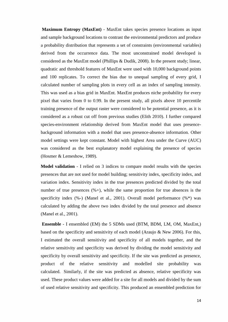
Maximum Entropy (MaxEnt) - MaxEnt takes species presence locations as input

and sample background locations to contrast the environmental predictors and produce

a probability distribution that represents a set of constraints (environmental variables)

derived from the occurrence data. The most unconstrained model developed is

considered as the MaxEnt model (Phillips & Dudik, 2008). In the present study; linear,

quadratic and threshold features of MaxEnt were used with 10,000 background points

and 100 replicates. To correct the bias due to unequal sampling of every grid, I

calculated number of sampling plots in every cell as an index of sampling intensity.

This was used as a bias grid in MaxEnt. MaxEnt produces niche probability for every

pixel that varies from 0 to 0.99. In the present study, all pixels above 10 percentile

training presence of the output raster were considered to be potential presence, as it is

considered as a robust cut off from previous studies (Elith 2010). I further compared

species-environment relationship derived from MaxEnt model that uses presence-

background information with a model that uses presence-absence information. Other

model settings were kept constant. Model with highest Area under the Curve (AUC)

was considered as the best explanatory model explaining the presence of species

(Hosmer & Lemeshow, 1989).

Model validation - I relied on 3 indices to compare model results with the species

presences that are not used for model building; sensitivity index, specificity index, and

variation index. Sensitivity index in the true presences predicted divided by the total

number of true presences (%+), while the same proportion for true absences is the

specificity index (%-) (Manel et al., 2001). Overall model performance (%*) was

calculated by adding the above two index divided by the total presence and absence

(Manel et al., 2001).

Ensemble - I ensembled (EM) the 5 SDMs used (BTM, BDM, LM, OM, MaxEnt,)

based on the specificity and sensitivity of each model (Araujo & New 2006). For this,

I estimated the overall sensitivity and specificity of all models together, and the

relative sensitivity and specificity was derived by dividing the model sensitivity and

specificity by overall sensitivity and specificity. If the site was predicted as presence,

product of the relative sensitivity and modelled site probability was

calculated. Similarly, if the site was predicted as absence, relative specificity was

used. These product values were added for a site for all models and divided by the sum

of used relative sensitivity and specificity. This produced an ensembled prediction for

15

every site, where probability greater than 0.5 was considered as presence, else

absence. I further, calculated the sensitivity, specificity and overall performance for

the ensemble model. As the BDM is based on exclusive density which might outfit

other models, I modelled another ensemble (EM-BDM) with only 4 SDMs (BTM,

LM, OM, MaxEnt) and validated the model in similar way. Statistical and GIS

analysis was performed using R. 3.0.2 and ArcMap 10.2 respectively.

Diversity parameters:

With the collected information, ‘Species accumulation curves’ and ‘Rank abundance

plots’ (RA) were generated using Microsoft excel 2010, for all the vegetation strata.

RAs were generated to infer commonness, rarity and evenness for 13 different

categories of invasion (Appendix S2 A). Measures of diversity like species richness,

Shannon diversity and species evenness were also calculated for each sampling plot

using R.3.0.2.

NMDS: To visualize the difference in community ordination between species and 120

sampled sites, non-metric multidimensional scaling (NMDS) was used. For plotting

NMDS on the species-sites matrix, Bray-Curtis dissimilarity matrix was calculated

(distance = "bray"). The rationale behind the selection of Bray-Curtis index was that

this index is based on “the sum of the differences in attributes between each pair of

sites divided by the sum of the attributes for the pairs of sites” (Abreu and Durigan

2011). Species abundance data was used from each plot with four divisions Native

(uninvaded plots), Lantana (plots invaded with Lantana only), Pogostemon (plots

invaded with Pogostemon only), L+P (plots invaded with both the species).

The NMDS was calculated with the VEGAN package in R (Oksanen et al. 2009),

which aims to find a stable solution using several random starts. To find a stable

solution, 50 permutations (trymax = 50) and 3 axes (k = 3) were selected for the

analysis. All the data analyses were made in R 3.0.2 (R Development Core Team

2009).

CCA: After visualising the invaded and uninvaded plots in NMDS, Canonical

Correspondence Analysis (CCA) was done to relate the distribution of plant species

composition with the environmental predictors (Guisan et al. 1999, Braak 1987). CCA

was performed using BiodiversityR package in R 3.0.2 (Kindt and Kindt 2016). A

total of 1000 permutations were set and environmental variables which explained

16

maximum proportion of variance were selected for the analysis (Abundance of

Pogostemon (PogoAbun), Abundance of Lantana (LanAbun), Soil moisture (Smoist),

Light on ground (lightGr), land surface temperature of April (ran_aprlst) and

deciduousness of the forest (ran_ndvidi)).

Comparing response variables along the gradient of plant invasion

using linear model (ANOVA)

To establish the correlation of lantana and pogostemon abundances with diversity

parameters and soil nutrients, native species richness, richness of rare species,

Shannon-Weaver diversity, evenness, organic carbon, potassium and soil moisture

content (response variables) were calculated for 120 sampling plots. Difference in the

response variables for plots with single and multiple invasions as compared to native

plots were estimated using the Linear Models (LMs) in ANOVA framework (Werts

and Linn 1970, Bolker 2008). Thus, un-invaded plot (NPNL) was taken as contrast or

reference plot, against which the beta values for each plot represented the degree of

variation and p-value represented the significance of it. These response variables were

assessed for multicollinearity and checked for pearson’s correlation. The analyses

were computed in R. 3.0.2.

17

Field view 5: Prof Qamar Qureshi and Dr Y.V.Jhala visiting a

sampling plot in a low lantana abundance area.

18

CHAPTER THREE: RESULTS

Distribution of Invasive plants

Out of the 56 km2 surveyed area, 40 km

2 (71%) and 37 km

2 (66%) was found to be

invaded by lantana and pogostemon; while, 14 km2 (29%) and 20 km

2 (34%) was

devoid of their invasion, respectively. Results of 120 plots intensively surveyed for

understanding the physiological parameters, germination success and environmental

stress are summarized in table 2.

Lantana camara complex:

Mechanistic models: BTM best explained lantana presence to be constrained by

evapotranspiration rate of summer (<130 mm/day), light availability and dry stress (<

37°C); as other constrains did not limit the study area. It could only classify 53% of

presence and 29% of absence of lantana. BDM on other hand best explained lantana

presence as a function of nearby lantana density, and then, by constrains explained by

BTM. BDM could classify 94% of lantana presence and 97% of its absence in the

study area.

Correlative model: LM best explained lantana cover to increase with increase in

summer temperature, Annual temperature, deciduousness of forest and decrease with

distance from canopy opening and forest patch edge. It could classify 95% and 13% of

lantana presence and absence, respectively. OM best explained lantana presence to

increase with increase in summer temperature, Annual temperature, deciduousness of

forest, distance from forest patch edge (insignificant) and decrease with distance from

canopy opening and post-monsoon NDVI. OM could classify 97% presence and 16%

absence of lantana. MaxEnt best modelled lantana presence with increase in summer

temperature, Annual temperature, deciduousness of forest, distance from forest patch

edge (insignificant) and decrease in distance from canopy opening and post-monsoon

NDVI. It could classify 76% and 28% of lantana presence and absence. Relative

importance of the environmental covariates for explaining lantana presence in LM,

OM and MaxEnt is summarized in table 3. However the explanatory power of LM and

OM was low (LM R2 value =0.18, OM R

2 value=0.13), while that for MaxEnt was

19

relatively higher (AUC=0.59). Details on stepwise selection of different models for

each correlative SDM is provided in the Appendix S1 D.

Table 2: Physiological parameters, germination success and environmental stress

threshold of lantana and pogostemon in the study area; used for deriving the

mechanistic model of species.

Mechanisms Lantana Pogostemon Source

Physiology

Body water content (g) 748 (18-

1953)

554 (40-

1403)

Present

study

Body temperature (°C) 29 (22-38) 25 (21-33) Present

study

Evapotranspiration

threshold (mm/day)

< 130 < 95 Present

study

Germination

Germination temperature

(Annual average

temperature(°C))

22 (15-38) 19 (16-33) CABI

Germination moisture throughout throughout CABI

Light (canopy density) NDVI <

0.40

NDVI <

0.43

Present

study

Stress

Heat stress (Maximum

temperature of warmest

month (°C))

> 41 > 40.5 Wijayaba

ndara et al

2013

Cold stress (Minimum

temperature of coldest

month (°C))

< 5 < 5 Wijayaba

ndara et al

2013

Dry stress (Soil surface

temperature (°C))

>37 >33 Present

study

Wet stress (maximum

rainfall of the wettest

month (mm))

>1195 >1280 Present

study

20

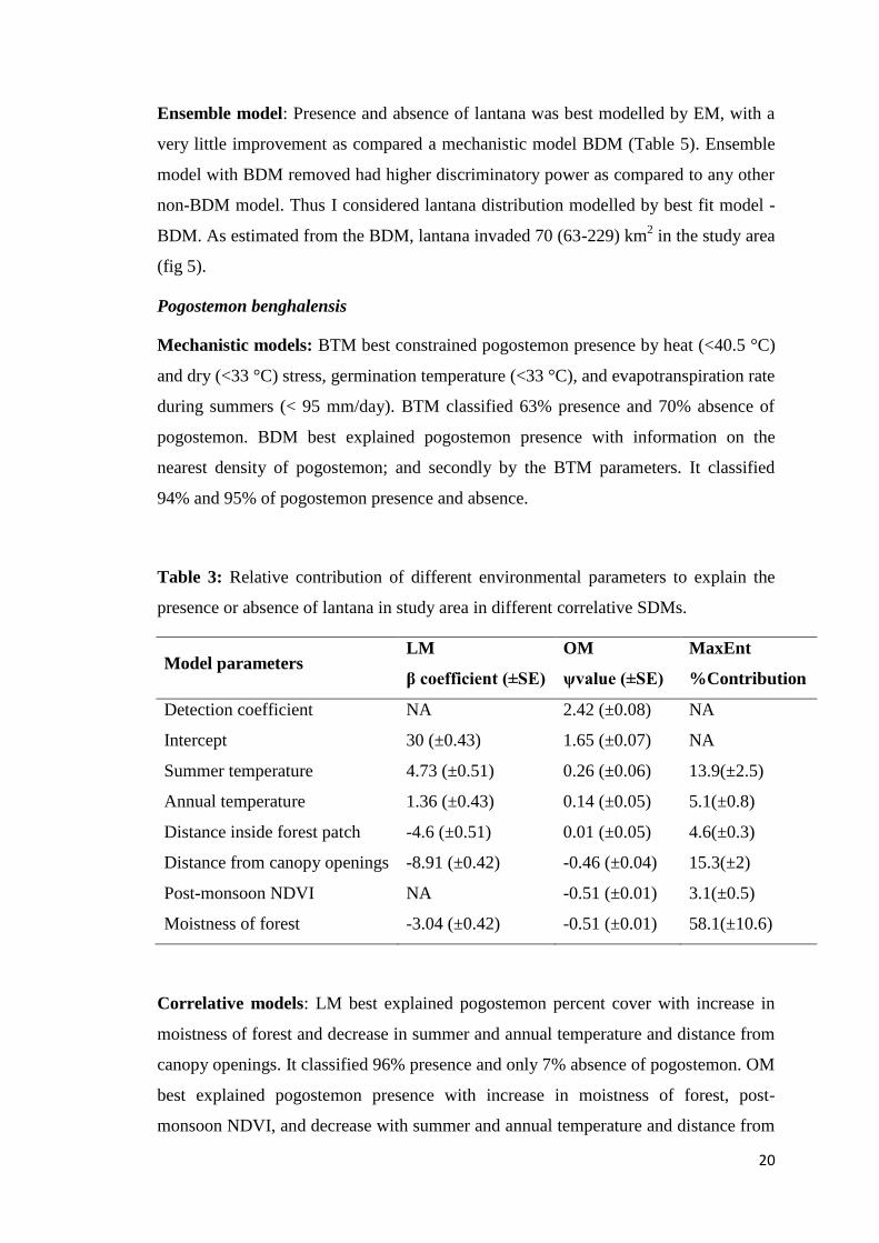
Ensemble model: Presence and absence of lantana was best modelled by EM, with a

very little improvement as compared a mechanistic model BDM (Table 5). Ensemble

model with BDM removed had higher discriminatory power as compared to any other

non-BDM model. Thus I considered lantana distribution modelled by best fit model -

BDM. As estimated from the BDM, lantana invaded 70 (63-229) km2 in the study area

(fig 5).

Pogostemon benghalensis

Mechanistic models: BTM best constrained pogostemon presence by heat (<40.5 °C)

and dry (<33 °C) stress, germination temperature (<33 °C), and evapotranspiration rate

during summers (< 95 mm/day). BTM classified 63% presence and 70% absence of

pogostemon. BDM best explained pogostemon presence with information on the

nearest density of pogostemon; and secondly by the BTM parameters. It classified

94% and 95% of pogostemon presence and absence.

Table 3: Relative contribution of different environmental parameters to explain the

presence or absence of lantana in study area in different correlative SDMs.

Model parameters LM OM MaxEnt

β coefficient (±SE) ψvalue (±SE) %Contribution

Detection coefficient NA 2.42 (±0.08) NA

Intercept 30 (±0.43) 1.65 (±0.07) NA

Summer temperature 4.73 (±0.51) 0.26 (±0.06) 13.9(±2.5)

Annual temperature 1.36 (±0.43) 0.14 (±0.05) 5.1(±0.8)

Distance inside forest patch -4.6 (±0.51) 0.01 (±0.05) 4.6(±0.3)

Distance from canopy openings -8.91 (±0.42) -0.46 (±0.04) 15.3(±2)

Post-monsoon NDVI NA -0.51 (±0.01) 3.1(±0.5)

Moistness of forest -3.04 (±0.42) -0.51 (±0.01) 58.1(±10.6)

Correlative models: LM best explained pogostemon percent cover with increase in

moistness of forest and decrease in summer and annual temperature and distance from

canopy openings. It classified 96% presence and only 7% absence of pogostemon. OM

best explained pogostemon presence with increase in moistness of forest, post-

monsoon NDVI, and decrease with summer and annual temperature and distance from

21

canopy openings. It classified 88% and 19% of pogostemon presence and absence.

While, MaxEnt modelled pogostemon presence with increase in moistness of forest,

post-monsoon NDVI, and decrease with summer and annual temperature and distance

from canopy openings and patch edge. It could discriminate 90% presence and 23%

absence of pogostemon. Relative importance of these covariates for explaining

pogostemon presence is summarized in table 4.

Ensemble model: Pogostemon presence and absence was best discriminated by

ensemble models (94% presence and 95% absence; Figure 6). EM-BDM lost its

discriminatory accuracy when density information was removed from it (52%

presence and 67% absence).

Table 4: Relative contribution of different environmental parameters to explain the

presence or absence of pogostemon in study area in different correlative SDMs.

Model parameters LM OM MaxEnt

β coefficient (±SE) ψ value (±SE) %contribution

Detection coefficient NA 3.28 (±0.12) NA

Intercept 38.4 (±0.49) 0.82 (±0.04) NA

Summer temperature -6.76 (±0.59) -0.79 (±0.05) 19.1(±3.2)

Annual temperature NA NA 0.5(±0.1)

Distance inside forest patch -4.82 (±0.59) -0.46 (±0.04) 9.1(±1.7)

Distance from canopy

openings -3.6 (±0.49) -0.33 (±0.04) 4.3(±0.6)

Post-monsoon NDVI NA 0.45 (±0.14) 0.5(±0.1)

Moistness of forest 18.52 (±0.49) 0.45 (±0.14) 66.5(±11.2)

22

Table 5: Comparing the discriminatory power of SDMs for differentiating species’

presence and absence using the sensitivity index (%+), specificity index (%-) and

model performance (%*). Darker shade represents stronger index. Area estimated to

be invaded by each SDM is given separately.

Model Lantana camara Pogostemon benghalensis

%+ %- %* Area (km2) %+ %- %* Area (km

2)

LM 0.95 0.13 0.69 212 0.96 0.07 0.65 220

OM 0.97 0.16 0.74 229 0.88 0.19 0.71 225

MaxEnt 0.76 0.28 0.74 221 0.90 0.23 0.89 176

BTM 0.53 0.29 0.52 139 0.63 0.70 0.64 124

BDM 0.94 0.97 0.95 63 0.94 0.95 0.95 69

EM 0.95 0.95 0.95 70 0.94 0.95 0.95 79

EM-BDM 0.75 0.59 0.71 148 0.52 0.67 0.57 92

Field view 6: Early morning visit to sample Sal forest for cover of invasive plants.

23

Figure 5: Lantana distribution modelled by Linear Model (LM), Occupancy Model

(OM), Maximum Entropy (MaxEnt), Biophysical Threhold Model (BTM),

Biophysical Density Model (BDM) and Ensemble of all these models (Ensemble) in

the study area

24

Figure 6: Pogostemon distribution modelled by Linear Model (LM), Occupancy

Model (OM), Maximum Entropy (MaxEnt), Biophysical Threshold Model (BTM),

Biophysical Density Model (BDM) and Ensemble of all these models (Ensemble) in

the study area.

25

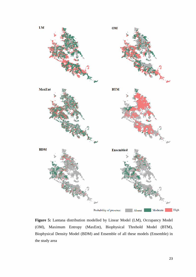
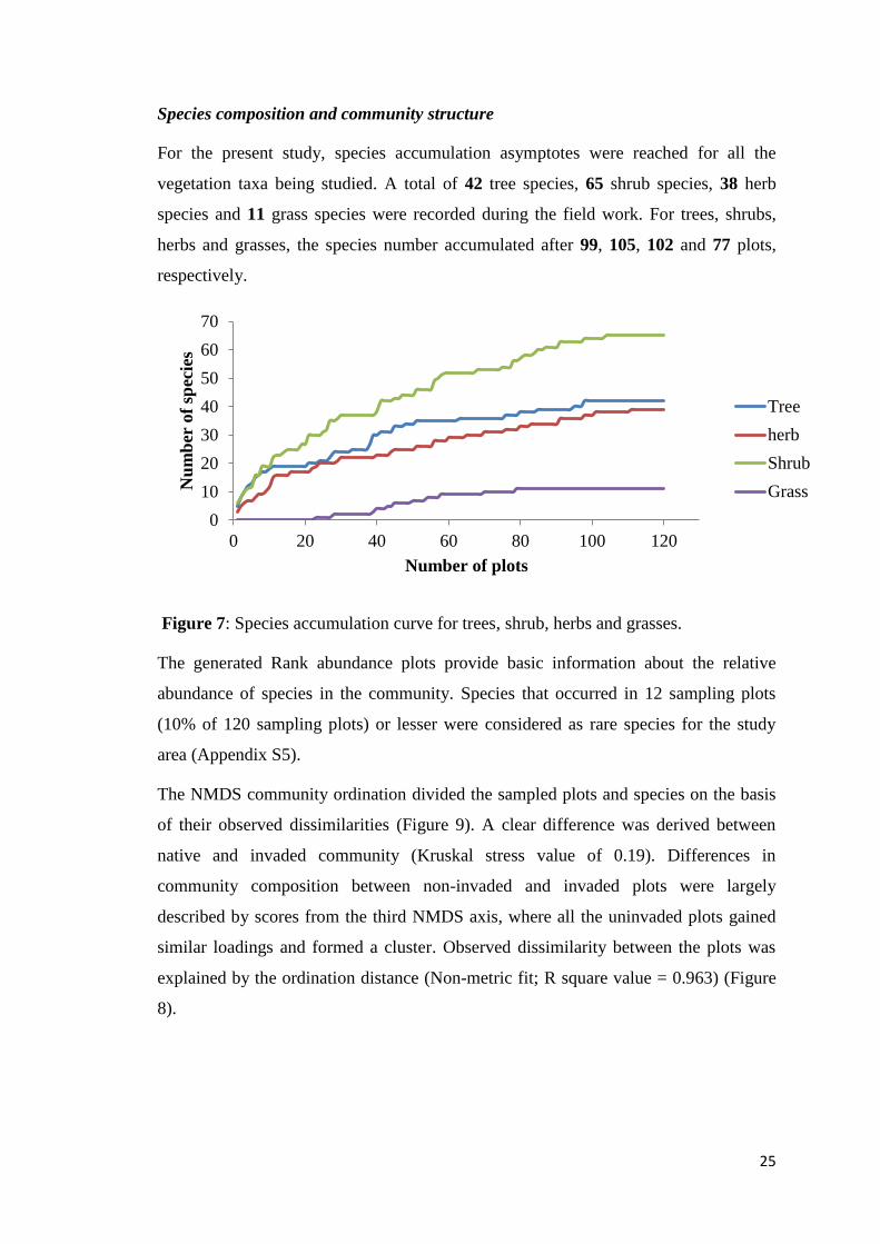
Species composition and community structure

For the present study, species accumulation asymptotes were reached for all the

vegetation taxa being studied. A total of 42 tree species, 65 shrub species, 38 herb

species and 11 grass species were recorded during the field work. For trees, shrubs,

herbs and grasses, the species number accumulated after 99, 105, 102 and 77 plots,

respectively.

Figure 7: Species accumulation curve for trees, shrub, herbs and grasses.

The generated Rank abundance plots provide basic information about the relative

abundance of species in the community. Species that occurred in 12 sampling plots

(10% of 120 sampling plots) or lesser were considered as rare species for the study

area (Appendix S5).

The NMDS community ordination divided the sampled plots and species on the basis

of their observed dissimilarities (Figure 9). A clear difference was derived between

native and invaded community (Kruskal stress value of 0.19). Differences in

community composition between non-invaded and invaded plots were largely

described by scores from the third NMDS axis, where all the uninvaded plots gained

similar loadings and formed a cluster. Observed dissimilarity between the plots was

explained by the ordination distance (Non-metric fit; R square value = 0.963) (Figure

8).

0

10

20

30

40

50

60

70

0 20 40 60 80 100 120

Nu

mb

er o

f sp

ecie

s

Number of plots

Tree

herb

Shrub

Grass

26

Figure 8: Stress plot for Non-metric multidimensional scaling (Non metric fit,

R2=0.963).

27

Figure 9: Plant community ordination based on the observed dissimilarities in species-

sites matrix, using NMDS. Three major communities were derived which are Native

(uninvaded community), Lantana, Pogostemon, however, considerable overlap was

found when lantana and pogostemon occurred together (L+P).

Native

Lantana

Pogostemon

L+P

28

Canonical Correspondence Analysis (CCA): Six axes were obtained by

CCA for establishing correlation between native plant community (species variables)

and environmental variables. Due to high prevalence of rare species in sampling plots,

species which are present in twelve and/or lesser number of plots were eliminated

from the analysis. Among 6 components, first four explained 87% (0.87678) of the

variability (Table 6). A logical correlation was found between the plant community

structure, the abundance of invasive plants and other environmental parameters used

for CCA (Figure 10).

Table 6: Proportion of variations explained by different components of Canonical

Correspondence Analysis (CCA) and their eigen values.

CCA1 CCA2 CCA3 CCA4 CCA5 CCA6

Eigenvalue 0.1103 0.08799 0.05013 0.0306 0.02457 0.01464

Proportion Explained 0.3467 0.27646 0.15751 0.09614 0.0772 0.04602

Cumulative Proportion 0.3467 0.62313 0.78064 0.87678 0.95398 1

34 % of the variability was explained by the first component of CCA. Soil moisture

formed the major explanatory variable for component 1 (eigen value 0.1103), and

accounted for moist Sal forest with high soil moisture and less significance of lantana

presence (Table 7). Colebrokia oppositifolia, Flemingia macrophylla, Syzigium cumini

were positively correlated with the axis whereas, Mallotus phillipensis, Bauhinia

malabarica, Desmodium oojeinense, Smilax sp., Casearia graveolens, Trema

orientalis, were found to be correlated negatively. However, a significant negative

correlation was found for Ageratum conyzoides, which is another invasive species in

India and is a native species in Central America (Appendix S7).

Component 2 (eigen value 0.08799) which explained 27 percent of the variability was

dominated by abundance of Lantana and accounts for dry Sal forest with Lantana

presence (Table 7). Holarrhena antidysentrica, was found to be positively correlated

with Lantana and negative correlation was observed in Desmodium oojeinense and

Chloroxylon swietenia (Appendix S7).

15 % variability was explained by Component 3 (eigen value 0.05013) which was

dominated by land surface temperature of april, the axis primarily comprised of

decidious forest with significant presence of lantana and pogostemon (Table 7).

29

Holarrhena antidysentrica, Schleichera oleosa, Colebrokia oppositifolia, Ageratum

conyzoides, were few of the positively correlated species, whereas, Flemingia

semialata, Cordia myxa, Shorea robusta, Phoenix acaulis, Dendrocalamus strictus

and Asparagus racemosus were found to be negatively correlated with the axis.

Figure 10: Correlation of Native species with abundance of lantana (LanAbun),

pogostemon (PogoAbun), environmental parameters (Light intensity – lightGr,

deciduousness of forest - ran_ndvidiff) and edaphic factors (soil moisture- Smoist)

using Canonical Correspondence Analysis.

30

Component 4 and Component 5 which collectively explained 16 % of the total

variability (eigen values 0.0306, 0.02457, respectively) had no presence of Lantana or

Pogostemon and contained relatively moister Sal forest area (Table 7). Component 4

was interpreted to be relatively moist, cold and with high canopy cover (negative

correlation of land surface temperature and light on ground), whereas component 5

accounts for significant negative correlation with lantana and pogostemon and high

soil moisture. Species like Asparagus racemosus and Dendrocalamus strictus were

found to be positively correlated.

Component 6 with 4 % explanation (eigen value 0.01464) had significant correlation

with Pogostemon abundance and forest moistness (significant negative correlation

with NDVI difference). Species like Dendrocalamus strictus, Cassia fistula and Trema

orientalis were found to have negative correlation with the axis (Table 7).

Table 7: Relationship of environmental parameters with obtained six components of

CCA. Environmental parameters like Soil moisture, lantana abundance, pogostemon

abundance, light on ground, land surface temperature for the month of April,

deciduousness of the forest were selected.

Environmental parameter CCA1 CCA2 CCA3 CCA4 CCA5 CCA6

Soil moisture 0.85 -0.43 0.02 -0.03 0.32 0.01

Lantana Abundance 0.13 0.58 0.12 -0.03 -0.78 -0.16

Light on ground 0.04 0.44 -0.48 -0.58 -0.47 0.15

Land surface temperature (April) -0.13 0.06 0.54 -0.70 0.15 -0.42

Pogostemon Abundance -0.21 -0.52 0.04 -0.25 -0.76 0.21

Forest deciduousness -0.36 -0.38 0.04 -0.30 -0.12 -0.78

Comparing response variables along the gradient of plant invasion using linear

model (ANOVA)

Effect on native plant diversity: The diversity of native plants declined significantly

with lantana invasion (p< 0.001), pogostemon invasion (p<0.01) and invasion of both

species (p<0.05). However the decline in diversity was more with single species

31

invasion (lantana=1.04, pogostemon=1.43) when compared with both the species’

invasion together (1.47) (Table 8A).

Effect on native plant richness: The richness of native plants declined significantly

with lantana invasion (p< 0.001), pogostemon invasion (p<0.001) and invasion of both

species (p<0.01). However, the decline in richness was less with pogostemon invasion

(8.92) and when both the species’ invasion together (7.80) as compared to decline with

lantana invasion (4.75) (Table 8B).

Effect on native rare plant richness: The richness of native rare plants declined

significantly with lantana invasion (p< 0.001), pogostemon invasion (p<0.001) and

invasion of both species (p<0.001). However the decline in richness was less with

single species invasion (lantana=0.50±0.38, pogostemon=0.67±0.29) when compared

with both the species’ invasion together (0.40±0.36) (Table 8C).

Effect on native plant evenness: The evenness of native plants increased significantly

with lantana invasion (p< 0.05), pogostemon invasion (p<0.05) and insignificantly

with invasion of both species (p<0. 1). However the increase in evenness was more

with invasion of lantana (0.55) as compared to pogostemon (0.49) or both the species

together (0.46) (Table 8D).

Effect on soil chemicals: Soil moisture insignificantly increased with increase in

lantana cover (0.55, p>0.1), significantly increased with pogostemon (0.49, p<0.05)

and varied insignificantly when both the species occurred together (p>0.1) (Table 8E).

Among soil nutrients, organic carbon increased significantly with high lantana cover

(3.24, p<0.01) and increasing pogostemon cover (2.46, P<0.01) and varied

insignificantly (p>0.1) when both the species occurred together (Table 8F). Soil

potassium significantly increased with high pogostemon cover (4481, p<0.01) (Table

8G) and decreased with increased lantana (1736, p<0.05).

32

Table 8: Mean values of diversity and soil parameters arranged in the categories of

invasion at 10X10m scale. Different classes of no lantana (NL), low lantana (LL),

medium lantana (ML), high lantana (HL), no pogostemon (NP), low pogostemon (LP),

medium pogostemon (MP) and high pogostemon (HP) abundance are given. Here,

Green colour denotes the highest mean value, followed by orange, yellow and red the

least value. Bold values indicate a significant difference in the response variables as

compared with the uninvaded plot (NP, NL). The estimates on errors and significance

are given in Appendix S7.

A Shannon

NL LL ML HL

NP 1.84 1.61 1.23 1.04

LP 1.57 1.75 1.95 1.65

MP 1.54 1.66 1.47

HP 1.43 1.45

B Richness

NL LL ML HL

NP 17.60 7.00 5.00 4.75

LP 7.29 9.40 10.43 7.86

MP 8.71 8.67 7.80

HP 8.92 7.70

C Richness of rare species

NL LL ML HL

NP 5.33 0.50 0.50 0.50

LP 1.29 1.30 1.43 0.57

MP 0.82 1.67 0.40

HP 0.67 1.40

33

D Evenness

NL LL ML HL

NP 0.38 0.63 0.59 0.55

LP 0.64 0.55 0.59 0.55

MP 0.55 0.55 0.46

HP 0.49 0.49

E Soil moisture

NL LL ML HL

NP 10.48 9.71 8.69 7.51

LP 13.11 5.95 6.81 5.62

MP 10.40 7.57 7.84

HP 10.88 8.53

F Organic carbon

NL LL ML HL

NP 1.81 1.89 1.92 3.24

LP 2.67 1.21 1.87 1.78

MP 2.46 2.11 2.46

HP 2.46 1.71

G Potassium

NL LL ML HL

NP 2955 2179 1841 1736

LP 2984 3337 3289 3504

MP 3240 2964 3478

HP 4481 3593

This significant decline in species richness and diversity with increase in lantana and

pogostemon cover (single species invasion) indicates towards the biotic

homogenization of the plant community.

34

CHAPTER FOUR: DISCUSSION AND CONCLUSION

The present study aimed to look at the effects of two invasive plants, a non-native

invasive, Lantana camara complex and a native invasive, Pogostemon benghalensis

and the difference in plant community structure with an increasing magnitude of their

invasion. In addition to this, three hypotheses which are biotic homogenization

hypothesis (BH), intermediate disturbance hypothesis (IDH) and invasional meltdown

hypothesis (IMH) were tested (Simberloff and Von Holle 1999, Connell 1978,

McKinney 1999). To test these hypotheses, the study was designed so as to control the

effect of extrinsic factors like anthropogenic disturbances and establish a cause-effect

relationship of altered community structure with invasive species (lantana and

pogostemon).

Distribution of Invasive plants

For the first objective, the study area was extensively surveyed for the percent cover of

lantana and pogostemon, which were later modelled using different Species

Distribution Models (SDMs). It was found that lantana has invaded habitats that are

changed by anthropogenic modifications like tourism roads, fire control lines and

water bodies (Table 3). It has also invaded the edges of forest patch more as compared

to the core, suggesting that fragmentation can further elevate the invasion, particularly

done by anthropogenic modifications. Lantana distribution was however restricted due

to remote, moist forest patches, and due to climatic heat and edaphic dry stress.

Pogostemon on the other hand is best explained by moistness of forest patch, lower

summer temperature and habitat opening by anthropogenic factors (Table 4). It is

restricted due to climatic heat and edaphic dry stress, and remote deciduous forest

(Table 4). Thus, in addition to the precise distribution map made by ensembling the

correlative and mechanistic SDMs, it also provides a holistic understanding of species

spatial ecology and the likely effects of any conservation management action taken by

the concerned stakeholder.

In one of the most intensive survey based comparison of correlative, mechanistic and

ensemble models at microscale for native and non-native invasive weedy plants I

found mechanistic models and ensemble models outperformed correlative models.

However, if density information from the ensemble model was removed (as it is most

of the times unavailable), MaxEnt model had the best performance, but under-

35

predicted the species’ absence. Poor performance of linear modelling (LM) and

occupancy modelling (OM) amongst the correlative models can potentially be due to

fitting a linear function with the most significant correlated parameter (distance from

canopy openings in the present case). In areas where both the species are absent due to

parameters that are less significantly correlated (temperature and moistness of the

forest in present case), the former takes over the later, producing pseudo-presence and

under-fitting the absences. As a result I got a higher sensitivity index but a very poor

specificity index. In case of MaxEnt, it fits non-linear and interactive relations with the

covariates that checks for the spatially interacting constraints (Phillips & Dudik,

2008). Hence, the specificity index of MaxEnt was highest in comparison with LM

and OM.

Mechanistic BTM model on other hand considers extreme constraints that represent

localized range of the species, due to which few areas within the range those are

devoid of invasion may be misclassified as presence. This is resolved when density

informed from intraspecific distances are incorporated to interact with the BTM.

Though BDM that are produced by such interactions, need exhaustive ground survey,

turned to best explain the species presence and absence. The sensitivity and specificity

of BDM outnumbered any other model, so much so that the ensemble of all these

models was similar to the BDM. Ensemble models with the BDM removed produced

sensitivity and specificity index, which was less than either sensitivity or specificity

index of other SDMs. Hence, due to intensive information on microscale densities that

interact with mechanistic models, I contradict previous studies who reported poor

performance of mechanistic models as compared to correlative models (e.g. Buckley

et al 2010). Ensemble models based on such information not only produces a precise

distribution estimate, but also provides an insight into how species are limited in the

ecosystems. Particularly in case of invasive plants, such information can assist in

taking adaptive decisions for invasive species management.

Species composition and community structure

For achieving the second objective, diversity parameters were derived and community

ordination was carried out. Rank abundance plots obtained from the study clearly

indicate the presence of more than 50 % of rare species (27 trees, 38 shrubs and 28

herbs). These species were termed ‘rare’ because of their occurrence in less than 10

percent of the sampled plots (<12 plots), however, this connotation of rarity is defined

36

for the present study and does not pertain to the rare status of the species, per se.

These basic diagnostic graphs also provided insights about the low evenness of the

study area which can be attributed to Sal forest itself, since it is one of the most

homogenous forest types in the tropical India (Champion and Seth 1968).

Based on the observed dissimilarity, visual demarcation of invaded and un-invaded

communities was depicted in the NMDS plot. This assessment was supported by the

Kruskal stress value of 0.19, which indicates a good fit for the ordination (Figure 8).

Similar results were obtained when, correlation between native plant species and

independent explanatory variables like abundance of lantana and pogostemon, edaphic

factors and canopy opening was established using Canonical Correspondence analysis

(CCA).

In CCA, Component 1 and 2, which collectively explained 62 % of the variability in

the dataset accounted for soil moisture and presence of lantana. Palatable species like

Bauhinia malabarica, Caseraria graveolens, Smilax sp., Schleichera oleosa, Miliusa

tomentosa, Ziziphus rugosa, Mallotus phillipensis were negatively loaded on these

axes. This negative relationship with palatable species might indicate towards

depletion of quality of forage available and facilitation of weedy species like

Colebrokia oppositifolia which is positively correlated with the first component

(Appendix S7).

With the presence of lantana and pogostemon both, negative relationship was obtained

for species like Ziziphus rugosa, Smilax, Asparagus racemosus, Dendrocalamus

strictus, Phoenix acaulis, Shorea robusta, Cordia myxa and Flemingia semialata on

component three. Asparagus racemosus (Shatavar) was found to be a rare species for

sal forest in the study area and is proven to have many medicinal properties (Mandal et

al., 2000), depiction of a negative relationship with Shorea and Asparagus raises

concern as it might indicate towards a decline in the population of the species in the

longer run. Positive correlation of component three with another invasive species i.e,

Ageratum conyzoides, supports the argument of Invasional meltdown being studied.

Component four and five indicated towards positive relationship obtained for above

mentioned palatable and rare species. Sampling plots with dense canopies, low land

surface temperature and relatively high moisture content were present in the accounted

component. Negative loadings with lantana and pogostemon abundance in the

37

component might refer to the failure of their establishment in these forest patches.

Component six of CCA, explained the presence of pogostemon and negative

correlation with Trema orientalis, Cassia fistula, Chloroxylon swietenia and

Desmodium oojeinense was obtained.

Biotic homogenization hypothesis

Biotic homogenization is a phenomenon where species diversity of a community

declines and forms a simpler community with less number of species. In such a

scenario, it is mostly few common species taking over the community assemblage and

rare species are mostly eliminated. In the present study, I observed the evenness of

plant assemblage to significantly increase with increase in either invasive species or

when both the species occur together (in low abundance of either one or both; Table

8). Significant increase in soil organic carbon with increase in the cover of single

invasive species was found. Similar to the theoretical predictions, we also observed

that elevated soil organic carbon potentially elicited facilitation of selective common

Fabaceae plants which in turn fixed nitrogen in the soil and facilitated lantana and

pogostemon.

A significant decline in diversity and richness and a significant increase in species

evenness and soil organic carbon support the notion that with increase in the

abundance of invasive species, simplification of the community assemblage takes

place, thus affirming the biotic homogenization hypothesis (Connell 1978).

Field view 7: Sal forest area with homogenized understorey, Phoenix acaulis (left)

and Holarrhena antidysentrica (right).

38

Invasional meltdown hypothesis

In the present study, increase in pogostemon decreased the diversity of native plants

and richness of rare plants; while increase in lantana decreased the native plant

diversity and rare species richness more substantially. It indicates that invasive plant

species are detrimental to the native plant diversity (Fensham et al., 1994; Swarbrick

et al., 1998; Batianoff and Butler, 2003; Sharma et al., 2005; Gooden et al., 2009).

When both the species were present in lesser proportion (10-50% cover of the plot)

there was an insignificant effect on the species diversity and richness as compared to

single invasion effect. However, presence of both invasive plants in higher proportions

(> 50% cover of the plot) and this combined effect might have exerted a significant

and substantial decline in the native plant diversity and richness of rare species (Table

8; Appendix S7). However, decline in the native diversity or richness can only

partially indicate towards invasional meltdown. As Gurevitch (2006) asserted that the

invasional meltdown is not mere additive effect of two species, which also happens to

be invasive, but a “cascade of positive feedbacks that accelerates its effects like a

snowball”. In current study, I found that when both the invasive species were present,

the native species diversity and richness declined, soil moisture decreased and organic

carbon and potassium increased (Table 8). Invasive species are globally known to

invade in potassium rich soils (Pieters & Baruch, 1997). I observed that in potassium

rich soils more native (Colebrookia oppositifolia) and non-native (Ageratum

conyzoides, Achyranthus aspera) weedy species in the plots with where pogostemon

and lantana were present. This indicates towards the paradigm of facilitation of

secondary invaders, but needs further validation. Hence, I observe an invasion centric

assemblage as a result of invasional meltdown brought by pogostemon and lantana in

the present study.

I see this Invasional meltdown as an alternate stable species assemblage to the native

stable species assemblage. Where, due to perturbation caused by synergistic

facilitation of invasive species the assemblage constrained by native species is shifted

to the assemblage constrained by invasive species. Though in the present study, I

might have unaccounted many complex interactions but, I observe a significant change

in species assemblage and potential species interactions due to presence of two

invasive plants. I take it a step ahead to propose that invasional meltdown can likely

shift the native regime of ecological assemblage to an invasive regime (Box1).

39

Box 1: Invasional meltdown to alternate

stable state (Scheffer and Carpenter 2003)

Schematic representation of shift from the native

ecosystem state (N) constrained by native species

assemblage (A) to invasion centered ecosystem

state (I) due to biological invasion in N, which is

initially constrained by native and invasive species

assemblage (B, C, D) but is later constrained by

invasive species assemblage alone (E). F1

represents the native stable state trajectory while

F2 represents an alternate invasive state trajectory

of an ecosystem that is influenced by the

‘attractors’ N and I.

Intermediate disturbance hypothesis:

Established negative impacts of invasive plants in the present study align with the

studies on biological invasions worldwide (Catford 2012, Shea 2004). So, it is safe to

assume biological invasions as a disturbance for native community. According to the

intermediate disturbance hypothesis, diversity of competing species is expected to

increase at intermediate frequencies of disturbance or environmental change (Connell

1978). However, in a review of more than 100 case studies, the diversity rarely peaked

(<20%) due to intermediate disturbances (Mackey and Currie 2001). This can be

attributed to the over-simplistic approach of IDH, it is mostly unable to inculcate, the

complexity associated with the magnitude and spatial context of disturbance regimes

(Chesson and Huntly, 1997). Studies that have affirmed IDH are many a times found

to have skewed study design and bias in selecting ecosystems where it IDH is likely to

be true (Fox 2013). In a theoretical framework, competition among the native species

is weakened by disturbances and should lead towards reduced species densities.

Similarly, this weakened competition should act upon all the taxa in a similar manner,

or should have an enhanced effect on rare species composition and their growth rate.

The difference in the growth rates between competitively superior and inferior species

A

B

C

D

E

N

Invasions

I I

Invasions

40

determines the rates of competitive exclusion; therefore intermediate disturbances are

affecting species’ abundance but not coexistence.

Even in the present study, I found a linear decrease in the native plant diversity,

richness and richness of rare plants (Table 8 A, B and C). When both the invasive

species co-occurred at lesser densities (<50% of the plot), I observed an insignificant

rise in native plant diversity, but it was still lesser when compared with the uninvaded

areas. For areas, where both the plants were present in high magnitude, all the

diversity and richness parameters significantly decreased. Hence, I do not see any

significant peak in diversity due to intermediate invasions (single as well as multiple);

rather observe a substantial decline as compared to the un-invaded community.

Sticking to the constraints of time and issue with seasonality of dataset, the study

indicates towards a linear decline in diversity with increasing invasion magnitude,

hence, I reject the intermediate disturbance hypothesis in the spatial context. However,

community and disturbance regime are complex phenomenon and should essentially

be observed over a long span of time, so, I also suggest that the patterns of community

organization with respect to biological invasions should be testified over a long span

of time.

With such conclusions and significant rejection power, scholars (e.g. Fox 2013) might

classify present study to have accepted a sceptic hypothesis. However, I confront to

the time constrain of present study, which might have potentially rejected the

intermediate disturbance hypothesis, with the assumption that biological invasions can

be placed in Joseph Hurd Connell’s definition of ‘disturbance’ (e.g. Sheil and Burslem

2013).

Conclusion, personal observations and management implication:

The current study clearly points out the factors associated with invasion of Lantana

camara and Pogostemon benghalensis in drier Sal forest of Kanha National Park.

Lantana invasion was primarily explained by canopy openings and edges of forest and

was constrained by moist forest patches, drier soil. On the other hand, pogostemon

invasion was explained by canopy openings, moist forest and relatively colder forest

floor. Pogostemon distribution was primarily constrained with deciduousness of forest.

With the current comparison among various species distribution models, I found that

mechanistic models outperform correlative models at finer scales and ensembling

41

these models can not only provide better distribution maps but also informs about

ecological constraints of the species.

Coming to the community organization and effect of single and multiple invasions on

native plant community, I found that when lantana and pogostemon are present (either

single or together) in higher abundance, it triggers change in the species composition.

Being on field and taking close observations of the plant assemblage in that area, I

observed an increase in common species from family Fabaceae (Flemingia semialata,

Cassia fistula, etc; nitrogen fixers) with increased multiple invasions. I also observed

that it was only when these two species are present together that, other native weeds

(Colebrokia oppositifolia) and non-native (Ageratum conyzoides) species are present.

However, it can also be an artefact of my sampling and it needs further validation.

A dramatic change in soil chemicals (increase in soil organic carbon and decrease in

soil potassium) content is also found when uninvaded and twelve classes of invasion

were compared. But, I would refrain myself from coming to any conclusion, since

many other soil parameters like soil nitrogen, phosphorus, salinity and pH are yet to be

investigated.

With the present study, it is clear that invasive species impacts the community

structure and ecosystem functioning by not only the decline in diversity and richness

of the native species but also modification in the abiotic components like soil

nutrients.

I also found that multiple species invasion impacts richness of rare species more than

single species invasion. These rare species comprise of many palatable and medicinal

species like (Asparagus racemosus, Buchanania lanzan, Phyllanthus emblica and

Casearia graveolens). These species are not only providing forage to various

ungulates in the area, but can also indicate towards ecological health of the ecosystem.

Present study can be used as an evidence to prioritize immediate management

interventions inside Sal forest. In order to shift the invasion-centric assemblage to the

native species centred assemblage, consistent large scale and intensive efforts are

needed to revert back the areas invaded by multiple species. Field observations pooled

with the statistical outcomes suggest that intensive invasive species management is

required in areas where multiple invasions are present in lesser magnitude, as the

42

chances of extirpation of rare species in such areas are high. In this manner, a larger

area can be managed and preserved for native species.

Field view 8: Soil samples being processed on field (left) and Ninad sampling lantana

invaded area (right).

43

References

Araújo, M.B. and M. New, 2007. Ensemble forecasting of species

distributions. Trends in ecology & evolution, 22(1), pp.42-47.

Batianoff, G.N. and D.W. Butler, 2003. Impact assessment and analysis

of sixty-six priority invasive weeds in south-east Queensland. Plant Protection

Quarterly, 18(1), pp.11-15.

Batten, M. Katharine, M. Kate, M. Scow, Kendi F. Davies, and Susan

P. Harrison. 2006. "Two invasive plants alter soil microbial community

composition in serpentine grasslands." Biological Invasions 8, no. 2: 217-230).

Blackburn, T.M., P. Pyšek, S. Bacher, J.T. Carlton, R.P. Duncan, V.

Jarošík, J.R. Wilson, and D.M. Richardson, 2011. A proposed unified

framework for biological invasions. Trends in ecology & evolution, 26(7),

pp.333-339.

Blank, Robert R. 2008. "Biogeochemistry of plant invasion: a case

study with downy brome (Bromus tectorum)." Invasive Plant Science and

Management1, no. 2, 226-238.

Bolker, B.M., 2008. Ecological models and data in R. Princeton

University Press.

Buckley, L.B., M.C., Urban, M.J. Angilletta, L.G Crozier, L.J. Rissler,

and M.W. Sears, 2010. Can mechanism inform species’ distribution models?.

Ecology letters, 13(8), pp.1041-1054.

Cappuccino, N. and J.T. Arnason, 2006. Novel chemistry of invasive

exotic plants. Biology Letters, 2(2), pp.189-193.

Catford, J.A., C.C. Daehler, H.T. Murphy, A.W. Sheppard, B.D.

Hardesty, D.A. Westcott, M. Rejmánek, P.J. Bellingham, J. Pergl, C.C.

Horvitz, and P.E. Hulme, 2012. The intermediate disturbance hypothesis and

plant invasions: Implications for species richness and management.

Perspectives in Plant Ecology, Evolution and Systematics, 14(3), pp.231-241.

44

Champion, S.H. and S.K. Seth, 1968. A revised survey of the forest

types of India. A revised survey of the forest types of India.

Charles, Krebs J. 2009. "Ecology 6th Edition: The Experimental

Analysis of Distribution and Abundance." Person International Edition. San

Francisco, United States of America.

Chesson, P. and N. Huntly, 1997. The roles of harsh and fluctuating

conditions in the dynamics of ecological communities. The American

Naturalist, 150(5), pp.519-553.

Colautti, R.I., A. Ricciardi, I.A. Grigorovich, and H.J. MacIsaac, 2004.

Is invasion success explained by the enemy release hypothesis?. Ecology

Letters, 7(8), pp.721-733.

Connell, J.H., 1978. Diversity in tropical rain forests and coral reefs.

Science, 199(4335), pp.1302-1310.

Dassonville, N., S. Vanderhoeven, W. Gruber, and P. Meerts, 2007.

Invasion by Fallopia japonica increases topsoil mineral nutrient

concentrations. Ecoscience, 14(2), pp.230-240.

de Abreu, R.C. and G. Durigan, 2011. Changes in the plant community

of a Brazilian grassland savannah after 22 years of invasion by Pinus elliottii

Engelm. Plant Ecology & Diversity, 4(2-3), pp.269-278.

Ehrenfeld, J.G., 2009. Implications of Invasive Species for

Belowground Community and Nutrient Processes1.

Ehrenfeld, J.G., P. Kourtev, and W. Huang, 2001. Changes in soil

functions following invasions of exotic understory plants in deciduous forests.

Ecological applications, 11(5), pp.1287-1300.

Elith, J., M. Kearney, and S. Phillips, 2010. The art of modelling range‐

shifting species. Methods in ecology and evolution, 1(4), pp.330-342.

Elton, Charles S., 1958. "The ecology of invasions by plants and

animals." Methuen, London 18.

Ens, E.J., J.B. Bremner, K. French, and J. Korth, 2009. Identification of

volatile compounds released by roots of an invasive plant, bitou bush

45

Chrysanthemoides monilifera spp. rotundata), and their inhibition of native

seedling growth. Biological invasions, 11(2), pp.275-287.

Ens, E.J., K. French, and J.B. Bremner, 2009. Evidence for allelopathy

as a mechanism of community composition change by an invasive exotic

shrub, Chrysanthemoides monilifera spp. rotundata. Plant and Soil, 316(1-2),

pp.125-137.

Entekhabi, D., E.G. Njoku, P.E. O'Neill, K.H. Kellogg, W.T. Crow,

W.N. Edelstein, J.K. Entin, S.D. Goodman, T.J. Jackson, J. Johnson, and J.

Kimball, 2010. The soil moisture active passive (SMAP) mission. Proceedings

of the IEEE, 98(5), pp.704-716.

Entekhabi, D., E.G. Njoku, P.E. O'Neill, K.H., Kellogg, W.T. Crow,

W.N. Edelstein, J.K. Entin, S.D. Goodman, T.J. Jackson, J. Johnson, and J.

Kimball, 2010. The soil moisture active passive (SMAP) mission. Proceedings

of the IEEE, 98(5), pp.704-716.

Fensham, R.J., R.J. Fairfax, and R.J. Cannell, 1994. The invasion of

Lantana camara L. in forty mile scrub National Park, north Queensland.

Austral Ecology, 19(3), pp.297-305.

Fick, S.E. and R.J. Hijmans, 2017. WorldClim 2: new 1‐km spatial

resolution climate surfaces for global land areas. International Journal of

Climatology.

Fox, J.W., 2013. The intermediate disturbance hypothesis should be

abandoned. Trends in ecology & evolution, 28(2), pp.86-92.

Gioria, M. and B.A. Osborne, 2014. Resource competition in plant

invasions: emerging patterns and research needs. Frontiers in plant science, 5,

p.501.

Gioria, M., B. Dieterich, and B. Osborne, 2011, December. Battle of

the giants: primary and secondary invasions by large herbaceous species. In

Biology and Environment: Proceedings of the Royal Irish Academy (pp. 177-

193). Royal Irish Academy.

46

Gooden, B., K. French, P.J. Turner, and P.O. Downey, 2009. Impact

threshold for an alien plant invader, Lantana camara L., on native plant

communities. Biological conservation, 142(11), pp.2631-2641.

Green, P.T., D.J. O'Dowd, K.L. Abbott, M. Jeffery, K. Retallick, and R.

Mac Nally, 2011. Invasional meltdown: invader–invader mutualism facilitates

a secondary invasion. Ecology, 92(9), pp.1758-1768.

Guisan, A., S.B. Weiss, and A.D. Weiss, 1999. GLM versus CCA

spatial modeling of plant species distribution. Plant Ecology, 143(1), pp.107-

122.

Gurevitch, J., S.M. Scheiner, and G.A. Fox, 2006. The ecology of

plants (pp. 215-216).

Hanway, J.J. and H. Heidel, 1952. Soil analysis methods as used in

Iowa state college soil testing laboratory. Iowa agric, 57, pp.1-31.

Hejda, M., P. Pyšek, and V. Jarošík, 2009. Impact of invasive plants on

the species richness, diversity and composition of invaded communities.

Journal of Ecology, 97(3), pp.393-403.

Hines, J.E., 2006. PRESENCE 2: Software to estimate patch occupancy

and related parameters. USGS-PWRC.

Hosmer, D.W. and S. Lemeshow, 1989. Applied regression analysis.

New York, John Willey.

Hughes, F., P.M. Vitousek, and T. Tunison, 1991. Alien grass invasion

and fire in the seasonal submontane zone of Hawai'i. Ecology, 72(2), pp.743-

747.

Jhala, Y.V, Q, Qureshi and R, Gopal, 2015. Monitoring tigers, co-

predators and prey in India.

Johnson, J.B. and K.S. Omland, 2004. Model selection in ecology and

evolution. Trends in ecology & evolution, 19(2), pp.101-108.

Keane, R.M. and M.J. Crawley, 2002. Exotic plant invasions and the

enemy release hypothesis. Trends in Ecology & Evolution, 17(4), pp.164-170.

Kindt, R. and M.R. Kindt, 2016. Package ‘BiodiversityR’.

47

Krishen, P. 2013. Jungle trees of Central India.

Krivoruchko, K., 2012. Empirical bayesian kriging. ESRI: Redlands,

CA, USA.

MacKenzie, D.I., J.D. Nichols, G.B. Lachman, S. Droege, J. Andrew

Royle, and C.A. Langtimm, 2002. Estimating site occupancy rates when

detection probabilities are less than one. Ecology, 83(8), pp.2248-2255.

Mackey, R.L. and D.J. Currie, 2001. The diversity–disturbance

relationship: is it generally strong and peaked?. Ecology, 82(12), pp.3479-

3492.

Mandal, S.C., A. Nandy, M. Pal, and B.P. Saha, 2000. Evaluation of

antibacterial activity of Asparagus racemosus Willd. root. Phytotherapy

Research, 14(2), pp.118-119.

Manel, S., H.C. Williams, and S.J. Ormerod, 2001. Evaluating

presence–absence models in ecology: the need to account for prevalence.

Journal of applied Ecology, 38(5), pp.921-931.

Martin, R. Melissa W. Philip 2008. Tipping, and James O. Sickman.

"Invasion by an exotic tree alters above and belowground ecosystem

components. "Biological invasions, 8 1883-1894.

McGrath, D.A. and M.A. Binkley, 2009. Microstegium vimineum

invasion changes soil chemistry and microarthropod communities in

Cumberland Plateau forests. Southeastern Naturalist, 8(1), pp.141-156.

McKinney, M.L. and J.L. Lockwood, 1999. Biotic homogenization: a

few winners replacing many losers in the next mass extinction. Trends in

ecology & evolution, 14(11), pp.450-453.

Mu, Q., Zhao, M. and Running, S.W., 2013. MODIS Global Terrestrial

Evapotranspiration (ET) Product (NASA MOD16A2/A3). Algorithm

Theoretical Basis Document, Collection, 5.

Oksanen, J., F.G. Blanchet, R. Kindt, P. Legendre, P.R. Minchin, R.B.

O’hara, G.L. Simpson, P. Solymos, M.H.H. Stevens, H. Wagner, and M.J.

Oksanen, 2013. Package ‘vegan’. Community ecology package, version, 2(9).

48

Phillips, S.J. and M. Dudík, 2008. Modeling of species distributions

with Maxent: new extensions and a comprehensive evaluation. Ecography,

31(2), pp.161-175.

Pieters, A. and Z. Baruch, 1997. Soil depth and fertility effects on

biomass and nutrient allocation in jaraguagrass. Journal of Range

Management, pp.268-273.

Pyšek, P., V. Jarošík, P.E. Hulme, J. Pergl, M. Hejda, U. Schaffner, and

M. Vilà, 2012. A global assessment of invasive plant impacts on resident

species, communities and ecosystems: the interaction of impact measures,

invading species' traits and environment. Global Change Biology, 18(5),

pp.1725-1737.

Ray, A. and S. Quader, 2014. Genetic diversity and population

structure of Lantana camara in India indicates multiple introductions and gene

flow. Plant Biology, 16(3), pp.651-658.

Ray, A. and Ray, R., 2014. Rapid divergence of ecotypes of an invasive

plant. AoB Plants, 6, p.plu052.

Richards, C.L., O. Bossdorf, N.Z. Muth, J. Gurevitch, and M. Pigliucci,

2006. Jack of all trades, master of some? On the role of phenotypic plasticity in

plant invasions. Ecology letters, 9(8), pp.981-993.

Roy, D.P., V. Kovalskyy, H.K. Zhang, E.F. Vermote, L. Yan, S.S.

Kumar, and A. Egorov, 2016. Characterization of Landsat-7 to Landsat-8

reflective wavelength and normalized difference vegetation index continuity.

Remote Sensing of Environment, 185, pp.57-70.

Rozenstein, O., Z. Qin, Y. Derimian, and A. Karnieli, 2014. Derivation

of land surface temperature for Landsat-8 TIRS using a split window

algorithm. Sensors, 14(4), pp.5768-5780.

Sardans, J. and J. Peñuelas, 2015. Potassium: a neglected nutrient in

global change. Global Ecology and Biogeography, 24(3), pp.261-275.

Sax, D.F., J.J. Stachowicz, and S.D. Gaines, 2005. Species invasions:

insights into ecology, evolution and biogeography.

49

Sharma, G.P. and A.S. Raghubanshi, 2009. Lantana invasion alters soil

nitrogen pools and processes in the tropical dry deciduous forest of India.

Applied Soil Ecology, 42(2), pp.134-140.

Sharma, G.P., A.S. Raghubanshi, and J.S. Singh, 2005. Lantana

invasion: an overview. Weed Biology and Management, 5(4), pp.157-165.

Shea, K., S.H. Roxburgh, and E.S. Rauschert, 2004. Moving from

pattern to process: coexistence mechanisms under intermediate disturbance

regimes. Ecology letters, 7(6), pp.491-508.

Shea, Katriona, and P. Chesson, 2002."Community ecology theory as a

framework for biological invasions." Trends in Ecology & Evolution 17, no. 4

170-176.

Sheil, D. and D.F.R.P. Burslem, 2013. Defining and defending

Connell’s intermediate disturbance hypothesis: a response to Fox. Trends Ecol

Evol, 28, pp.571-572.

Simberloff, D. and B. Von Holle, 1999. Positive interactions of

nonindigenous species: invasional meltdown?. Biological invasions, 1(1),

pp.21-32.

Simberloff, D., 2006. Invasional meltdown 6 years later: important

phenomenon, unfortunate metaphor, or both?. Ecology Letters, 9(8), pp.912-

919.

Swarbrick, J.T., B.W. Willson, M.A. Hannan-Jones, 1998. Lantana

camara L., in: F. D. Panetta, R. H. Groves, and R. C. H. Shephard, (Eds.), The

Biology of Australian Weeds. RG and FJ Richardson, Melbourne, pp. 119-140.

Team, R.C., 2014. R: A language and environment for statistical

computing (Version 3.0. 2). R Foundation for Statistical Computing, Vienna,

Austria.

Ter Braak, C.J., 1987. The analysis of vegetation-environment

relationships by canonical correspondence analysis. In Theory and models in

vegetation science (pp. 69-77).

50

Thelen, G.C., J.M. Vivanco, B. Newingham, W. Good, H.P. Bais, P.

Landres, A. Caesar, and R.M. Callaway, 2005. Insect herbivory stimulates

allelopathic exudation by an invasive plant and the suppression of natives.

Ecology Letters, 8(2), pp.209-217.

Walkley, A. and I.A. Black, 1934. An examination of the Degtjareff

method for determining soil organic matter, and a proposed modification of the

chromic acid titration method. Soil science, 37(1), pp.29-38.

Werts, C.E. and R.L. Linn, 1970. A general linear model for studying

growth. Psychological Bulletin, 73(1), p.17.

Wijayabandara, S.M.K.H., K.M.G.G. Jayasuriya, and J.L.D.H.C

Jayasinghe, 2013. Seed dormancy, storage behavior and germination of an

exotic invasive species, Lantana camara L.(Verbenaceae). International

Research Journal of Biological Sciences, 2(1), pp.7-14.

Wilkinson, D.M., 1999. The disturbing history of intermediate

disturbance. Oikos, pp.145-147.

Wyckoff, P.H., A. Shaffer, B. Hucka, M. Bombyk, and A. Wipf, 2014.

No evidence of facilitation between invasive Rhamnus cathartica (European

buckthorn) and invasive earthworms in west central Minnesota. Pedobiologia,

57(4), pp.311-317.

Zar, J.H., 1999. Biostatistical analysis. Pearson Education India.

http://www.bbcearth.com/modal/episode-one/

http://www.cabi.org/

3

Appendix S1 : Datasheet for sampling Trees and Shrubs (including other invasive species like Hyptis and Ageratum, and highly abundant grasses, If

any.)

GPS Latitude (N) GPS Longitude (E) Lan% Pogo% Oth.Inv. Soil Temp. Range Terrain Ground Substrate Observer

A A Flat Sand

B B Beat Gentle slope Silt Date

C C Moderate slope Loam

D D Camp Steep Clay Time

E E Undulating/Rugged Rocky/Gravely

*Tree & Shrub Phenology codes: 1) no leaves (bare branches), 2) no leaves plus flowers 3) no leaves plus fruit, &flower, 4) leaf bud burst, 5) green leaves

6) green leaves + flower, 7) green leaves plus fruit (& flower), 8) brown leaves or burnt.

If in more than one phase, e.g. some in leaf & others in flower, mention "%" in each phenological phase, like 90% leaf and 10% flower.

Trees (in 10m x 10m) Shrubs ( in 10m x 10m) ID Species Number Phenology Canopy GBH height Species Number Phenology Height Canopy

4

Appendix S2: Datasheet for sampling Ground cover.

Recorder…………………………………… Date……………………… Time………………………. Field staff……………………………………………………

Beat: Plot:

Litter grass herbs

P L O T

Dry %

Green %

Sp (abundance)

% cover

Sp (abundance + phenology)

% cover

Dry %

Wet %

Dept h-cm

1 2 3 4 5 1 2 3 4 5 Bare

ground% Light

ground

A

a

b

c

B

a

b

c

C

a

b

c

D

a

b

c

E

a

b

c

Comments:

5

Appendix S3: Information on scale and source of remotely sensed data used for

present study

Dataset Scale and pre-processing Source

Worldclim data

representing Temperature

and Rainfall parameters

1 km (rescale to 100m by

PRISM)

Hijman 2017

Pre-monsoon and Post-

monsoon NDVI

30 m (Derived from the

near infrared and infrared

bands of Landsat 8 for

year 2016-2017)

Roy 2014

Soil Surface Temperature 100m (Derived from the

thermal bands of Landsat

8 for year 2016-2017)

Rozenstein 2014

Evapotranspiration rate 1 km Mu 2013

Soil Moisture Active

Passive

250m Entekhabi 2010

Tourism road, Water

streams, Forest type map

30m Kanha Management Plan

2010

6

Figure 11: Map showing the location of 24 grids (100X100m).

7

Appendix S4

Lantana occupancy model selection

Model AIC delta AIC

~Lantana presence ~ Distance from canopy openings +

Distance from edge + Summer temperature + Post-monsoon

NDVI + Moistness of forest + Annual temperature 5412.383 0

~Lantana presence ~ Post-monsoon NDVI 5554.35 141.9679

~Lantana presence ~ Moistness of forest 5554.35 141.9679

~Lantana presence ~ Distance from edge + Distance from

canopy openings + Summer temperature 5743.375 330.9928

~Lantana presence ~ Distance from canopy openings 5746.974 334.5919

~Lantana presence ~ Annual temperature 5813.334 400.9519

~Lantana presence ~ Distance from edge 5819.299 406.9164

~Lantana presence ~ Summer temperature 5819.743 407.3606

~Lantana presence~ Null Model 5822.37 409.9873

Pogostemon occupancy model selection

MODEL AIC delta AIC

~Pogostemon presence ~ Summer temperature + Distance

from edge + Distance from canopy openings + Post-monsoon

NDVI + Moistness of forest 5308.732 0

~Pogostemon presence ~ Post-monsoon NDVI 5716.492 407.7606

~Pogostemon presence ~ Moistness of forest 5716.492 407.7606

~Pogostemon presence ~ Distance from edge + Distance from

canopy openings + Summer temperature 5753.535 444.803

~Pogostemon presence ~ Summer temperature 5896.788 588.0561

~Pogostemon presence ~ Distance from canopy openings 5944.769 636.0374

~Pogostemon presence ~ Null model 6035.636 726.9046

~Pogostemon presence ~ Distance from edge 6037.437 728.7048

~Pogostemon presence ~ Annual temperature 6037.473 728.7416

8

Appendix S5: Rank abundance plots for tree, shrub and herb species in the study area

Figure a: Rank abundance plot for trees.

Figure b: Rank abundance plot for shrubs.

Figure c: Rank abundance plot for herbs.

020406080

100120140

020406080

100120140

Van

ch

ana

Ch

hin

d

Am

alta

s

Bam

bo

o

Laso

da

Gir

chi

Len

dia

chip

pa

goh

lar

Van

tam

bak

u

Bh

irra

Kam

ar k

as

Ch

idch

ida

Am

la

Gh

atia

Dh

ava

Van

su

li

Ku

mb

hi

Dad

her

a

Gh

ari

Pan

iab

illo

**

Van

mu

sli

Shrub

020406080

100

Tota

l nu

mb

er

of

sam

plin

g p

lots

Species name

Herb

9

Appendix S6: Loadings of various components of CCA on individual species.

Species CCA1 CCA2 CCA3 CCA4 CCA5 CCA6

Ageratum_conyzoides -0.95 -0.64 0.83 -0.24 0.14 -0.21

Asparagus_racemosus 0.43 0.47 -0.89 0.08 1.49 1.06

Bauhinia_malabarica -0.27 -0.20 0.27 -0.58 0.29 -0.35

Butea_monosperma 0.66 0.89 0.32 -0.38 1.21 0.17

Butea_superva 0.01 0.18 0.66 0.12 -0.12 0.65

Casearia_graveolens -0.69 -0.25 0.34 -1.02 0.33 1.20

Cassia_fistula 0.36 0.56 0.06 0.20 -0.40 -1.34

Chloroxylon_swietenia 1.29 -1.97 0.13 -1.42 0.08 -0.72

Colebrokia_oppositifolia 3.60 -1.92 0.96 -0.12 -0.14 -0.28

Cordia_myxa 1.18 0.06 -0.11 -0.64 1.01 1.38

Dalbergia_lanceolaria 0.84 0.95 0.13 -1.17 -1.32 0.33

Dendrocalamus_strictus 0.35 0.07 -0.69 0.27 1.19 -0.98

Desmodium_oojeinense -0.34 -1.45 0.39 -0.26 0.34 -0.47

Diospyros_meloanoxylon 0.29 0.16 0.00 -0.50 -0.36 0.44

Dud_bel -1.47 -0.09 0.50 2.69 0.56 1.14

Flemingia_macrophylla 2.38 -1.55 0.74 0.27 0.73 -0.36

Flemingia_semialata 0.04 0.06 -0.06 -0.09 -0.34 0.00

Gohlar 1.25 -2.12 -1.60 1.75 -0.44 0.14

Holarrhena_antidysentrica 0.99 1.50 1.21 0.33 0.20 -0.08

Kamar kas -0.07 1.06 -1.72 0.86 0.13 -1.27

Lagerstomia_parviflora 0.23 1.40 -0.04 -0.33 -0.09 0.65

Mallotus_phillipensis -0.24 -0.16 0.13 0.64 -0.43 0.12

Miliusa_tomentosa 0.65 -0.84 0.09 0.35 0.22 -0.02

Phoenix_acaulis 0.13 0.33 -0.44 0.28 -0.21 0.07

Schleichera_oleosa 1.03 -0.92 0.98 0.74 0.64 0.70

Shorea_robusta -0.07 0.11 -0.30 -0.25 0.18 0.06

Smilax -0.55 0.23 -0.92 -0.04 1.12 1.20

Syzygium_cumini 1.57 -1.50 0.13 -0.24 -0.05 0.35

Trema_orientalis -0.71 0.08 0.50 0.79 -0.17 -1.60

Urena_lobata -0.01 -1.09 0.05 -0.04 0.25 -0.28

V_tam -0.95 0.19 0.05 0.44 0.69 -0.01

ziziphus_rugosa 0.36 -0.53 -1.08 1.09 0.82 1.08

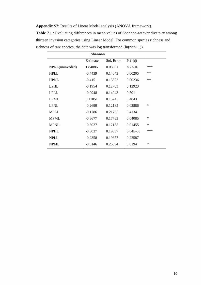
10

Appendix S7: Results of Linear Model analysis (ANOVA framework).

Table 7.1 : Evaluating differences in mean values of Shannon-weaver diversity among

thirteen invasion categories using Linear Model. For common species richness and

richness of rare species, the data was log transformed (ln(rich+1)).

Shannon

Estimate Std. Error Pr(>|t|)

NPNL(uninvaded) 1.84086 0.08881 < 2e-16 ***

HPLL -0.4439 0.14043 0.00205 **

HPNL -0.415 0.13322 0.00236 **

LPHL -0.1954 0.12783 0.12923

LPLL -0.0948 0.14043 0.5011

LPML 0.11051 0.15745 0.4843

LPNL -0.2699 0.12185 0.02886 *

MPLL -0.1786 0.21755 0.4134

MPML -0.3677 0.17763 0.04085 *

MPNL -0.3027 0.12185 0.01455 *

NPHL -0.8037 0.19357 6.64E-05 ***

NPLL -0.2358 0.19357 0.22587

NPML -0.6146 0.25894 0.0194 *

11

Appendix S7: Results of Linear Model analysis (ANOVA framework).

Table 7.2: Evaluating differences in mean values of native species’ richness among

thirteen invasion categories using Linear Model.

Richness

Estimate Std. Error Pr(>|t|)

NPNL(uninvaded) 2.8299 0.1025 < 2e-16 ***

HPLL -0.6332 0.1621 0.00016 ***

HPNL -0.6434 0.1537 5.87E-05 ***

LPHL -0.5643 0.1475 0.00022 ***

LPLL -0.4535 0.1621 0.0061 **

LPML -0.3261 0.1817 0.0755 .

LPNL -0.7928 0.1406 1.42E-07 ***

MPLL -0.5587 0.2511 0.02815 *

MPML -0.576 0.205 0.0059 **

MPNL -0.6619 0.1406 7.56E-06 ***

NPHL -1.1304 0.2234 1.75E-06 ***

NPLL -0.7544 0.2234 0.00102 **

NPML -1.0522 0.2988 0.00063 ***

12

Appendix S7: Results of Linear Model analysis (ANOVA framework).

Table 7.3: Evaluating differences in mean values of rare species’ richness among

thirteen invasion categories using Linear Model.

Richness of rare species

Estimate Std. Error Pr(>|t|)

NPNL(uninvaded) 1.7744 0.1309 < 2e-16 ***

HPLL -1.0353 0.2069 2.22E-06 ***

HPNL -1.3602 0.1963 3.29E-10 ***

LPHL -1.3988 0.1883 2.83E-11 ***

LPLL -1.0407 0.2069 1.99E-06 ***

LPML -1.0065 0.232 3.26E-05 ***

LPNL -1.1558 0.1795 3.51E-09 ***

MPLL -0.946 0.3205 0.00389 **

MPML -1.4971 0.2617 9.75E-08 ***

MPNL -1.3396 0.1795 2.38E-11 ***

NPHL -1.4278 0.2852 2.19E-06 ***

NPLL -1.7744 0.2852 9.75E-09 ***

NPML -1.4278 0.3815 0.0003 ***

13

Appendix S7: Results of Linear Model analysis (ANOVA framework).

Table 7.4: Evaluating differences in mean values of soil moisture content among

thirteen invasion categories using Linear Model.

Soil Moisture

Smoist Estimate Std. Error Pr(>|t|)

NPNL(uninvaded) 10.4847 0.95908 < 2e-16 ***

HPLL -1.9566 1.51643 0.19974

HPNL 0.39252 1.43861 0.7855

LPHL -4.8667 1.38035 0.00062 ***

LPLL -4.5362 1.51643 0.00345 **

LPML -3.6735 1.70026 0.03296 *

LPNL 2.6243 1.31584 0.04865 *

MPLL -2.9122 2.34925 0.21783

MPML -2.6427 1.91815 0.17116

MPNL -0.0879 1.31584 0.94688

NPHL -2.979 2.09026 0.15701

NPLL -0.7735 2.09026 0.71208

NPML -1.7919 2.79616 0.52299

14

Appendix S7: Results of Linear Model analysis (ANOVA framework).

Table 7.5: Evaluating differences in mean values of soil potassium (mg/kg) among

thirteen invasion categories using Linear Model.

K Estimate Std. Error Pr(>|t|)

NPNL(uninvaded) 2954.56 334.452 2.20E-14 ***

HPLL 638.484 528.815 0.22995

HPNL 1526.22 501.678 0.00295 **

LPHL 549.875 481.359 0.25586

LPLL 382.304 528.815 0.47129

LPML 334.853 592.92 0.57342

LPNL 29.066 458.864 0.94961

MPLL 9.644 819.237 0.99063

MPML 522.967 668.904 0.43604

MPNL 285.259 458.864 0.53549

NPHL -1218.9 728.921 0.0974 .

NPLL -775.74 728.921 0.28962

NPML -1113.4 975.087 0.25606

15

Appendix S7: Results of Linear Model analysis (ANOVA framework).

Table 7.6: Evaluating differences in mean values of soil organic carbon (%) among

thirteen invasion categories using Linear Model.

OC Estimate Std. Error Pr(>|t|)

NPNL(uninvaded) 1.80914 0.19702 3.61E-15 ***

HPLL -0.1029 0.31151 0.74175

HPNL 0.65394 0.29553 0.02904 *

LPHL -0.0309 0.28356 0.91336

LPLL -0.5957 0.31151 0.05852 .

LPML 0.05713 0.34928 0.87039

LPNL 0.86288 0.27031 0.00185 **

MPLL 0.30352 0.4826 0.53073

MPML 0.64722 0.39404 0.10342

MPNL 0.64872 0.27031 0.01813 *

NPHL 1.43477 0.42939 0.00115 **

NPLL 0.08052 0.42939 0.8516

NPML 0.10756 0.5744 0.85182

16

Appendix S8: List of shrubs recorded during field work.

SHRUB

Vernacular name Scientific name Vernacular name Scientific name

Ageratum Ageratum conyzoides Gud sukri Trema orientalis

Amaltas Cassia fistula Jamun Syzygium cumini

Amla Embelica officinalis Katjamun Syzygium salcifolium

Amti Bauhinia malabarica Kakai kata Bridelia retusa

Bamboo Dendrocalamus strictus Kamar kas

Band chippa Flemingia macrophylla Kari Miliusa tomentosa

Barga Kydia calycina Kasai/Khassi Bridelia retusa

Beeja Pterocarpus marsupium Katori Radermachera xylocarpa

Bhador Butea superva kosum Schleichera oleosa

Bhirra Chloroxylon swietenia Kumbhi Careya arborea

Char Buchcnania lanzan Lantana Lantana camara

Chhind Phoenix acaulis Lasoda Cordia myxa

Chidchida Acairanthus aspera Lendia Lagerstomia parviflora

chippa Urena lobata Mainhar Catunaregam spinosa

Churna ziziphus rugosa Mohin bela Bauhinia vahlii

chutni plant Antidesma acidum Mohti Colebrokia oppositifolia

Dadhera Bauhinia racemosa Palash Butea monosperma

Dhamin Grewia eriocarpa Paniabillo Gardenia latifolia

Dhandhani

Papdi Pavetta crassicaulis

Dhava Anogeissus latifolia Patavan Diospyros montana

Dhimar chnocarpus frutescens Pogostemon Pogostemon bengalhensis

Dhoban Dalbergia lanceolaria Ram datun Smilax

Dodhe bel

Saja Terminalia elliptica

Dudhi Holarrhena antidysentrica Sal Shorea robusta

dudhi bel

Sendur Mallotus phillipensis

Dudhi2 Writia tinctoria Shatavar Asparagus racemosus

Ghari Lannea coromandelica Tendu Diospyros meloanoxylon

Ghatia Ziziphus xylopyrus Tinsa Desmodium oojeinense

Girchi Casearia graveolens Van chana Flemingia semialata

17

Appendix S9: List of trees recorded during field work.

TREE

Vernacular

name Scientific name Vernacular name Scientific name

Amaltas Cassia fistula Kari Miliusa tomentosa

Amla Phyllanthus emblica Kasai/Khassi Bridelia retusa

Amti Bauhinia malabarica Katori Radermachera xylocarpa

Bamboo Dendrocalamus strictus Khamer Gmelina arborea

Barga Kydia calycina Kosum Schleichera oleosa

Beeja Pterocarpus marsupium Kumbhi Careya arborea

Bhilva Semecarpus anacardium Kurraiya(dudhi)

Holarrhena

antidysentrica

Bhirra Chloroxylon swietenia Lasoda Cordia myxa

Bhormal Hymenodictyon orixense Lendia Lagerstroemia parviflora

Char Buchcnania lanzan Mahua Madhuca latifolia

Churna Ziziphus rugosa Mohan bela Bauhinia vahlii

Dadhera Bauhinia racemosa Mundi Mitragyna parviflora

Dhamin/Dohan Grewia eriocarpa Pakri Ficus cupulata

Dhava Anogeissus latifolia Palash Butea monosperma

Dhoban Dalbergia lanceolaria Peepal Ficus religiosa

Ghari Lannea coromandelica Saja Terminalia elliptica

Ghari Lannea coromandelica Sal Shorea robusta

Ghatia zizyphus xylopyrus Sendur Mallotus philippensis

Haldu Haldina cordifolia Tendu Diospyros melanoxylon

Harra Terminalia chebula Thod Bauhinia roxburghiana

Jamun Syzigium cumini Tinsa Desmodium oojeinense

18

Appendix S10: List of herbs recorded during field work.

HERB

Vernacular name Scientific name Vernacular name Scientific name

Ageratum Ageratum conyzoides Jamun Syzigium cumini

Amla Phyllanthus emblica Kamarkas

Amti Bauhinia malabarica Khareta

Band chippa Flemingia macrophylla Khassi/Kasai Bridelia retusa

Beeja Pterocarpus marsupium Kosum Schleichera oleosa

Chidchida Acairanthus aspera Lantana Lantana camara

Churna Ziziphus rugosa Neela phool

Dhimar bel

Papdi bel

Dhoban Dalbergia lanceolaria Pogostemon Pogostemon bengalhensis

Dhudsi

Ram datun Smilax

Dodhe bel

Sal Shorea robusta

Doodhi bel

Sendur Mallotus philippensis

Dudhi

Holarrhena

antidysentrica Shatavar Asparagus racemosus

Ghatia Zizyphus xylopyrus Tendu Diospyros melanoxylon

Girchi Casearia graveolens Tinsa Desmodium oojeinense

Gohlar

Urena lobata Urena lobata

Harra Terminalia chebula Van chana Flemingia semialata

19

Response to comments for M.Sc. dissertation titled

‘Assessing the synergistic effect of two invasive plants on

native plant communities in Kanha National Park, Central

India’.

I thank the examiners for critical evaluation of my dissertation study and the

comments posed. Thank you for acknowledging the research work as an important

advance in the field of invasion ecology. Comments have been responded in a point

wise manner and attached overleaf.

______________________

Rajat Rastogi

XV M.Sc. Wildlife Science

Wildlife Institute of India.

Forwarded by:

_____________________

Prof Qamar Qureshi

Scientist-G

Co-supervisor

Date: 7 July 2017

Place: Dehradun

20

COMMENTS

1. Good work!

Thank you!

2. Without an experimental design, how do you know which direction the

causality lies? Ie. are invasive species able to colonize the less fertile areas rather

than cause the decline in fertility and associated diversity?

The ecological relationship between invasive plants and soil nutrients has been

a topic of major concern, lately. Recent studies have showed that with increase in

Lantana soil carbon and soil nitrogen has increased (Osunkoya & Perrett 2010). The

present case study was an observational experiment and not a manipulative one,

designed to compare the diversity parameters and edaphic factors in thirteen classes of

Invasion given in table 1. To achieve this, the forest type was selected to be Sal

(Shorea robusta) and extrinsic effects from canopy opening and different habitat type

were controlled. In this way, any change in diversity and edaphic factors was

considered to be an effect of invasive species only. However, I also agree that the

relationship thus found is correlative and needs manipulative experimentation, which

was beyond the scope of current study.

3. Discuss the limitations of intermediate disturbance hypothesis wrt

operational definition in discussion section

The suggestion is accepted and I have incorporated critiques of IDH in the

discussion (Page 39 and 40).

4. Replace all we with I, this is your thesis, you can put we in your research

paper.

The suggestion has been incorporated in the revised thesis.

5. How did you select them? Describe in methods section.

Selection of these 120 study plots was done after surveying 56km2 of Sal forest

area. It was based upon the percent cover of invasive species, Flat terrain, similar

canopy cover, distance from canopy openings, different forest types and water bodies.

The selection criterion was mentioned in the method section, in the draft sent to the

examiner.

6. Map with overlaid grids and selected grids would help in judging whether

sampling was biased in any way

Map has been added as a part of appendix S3

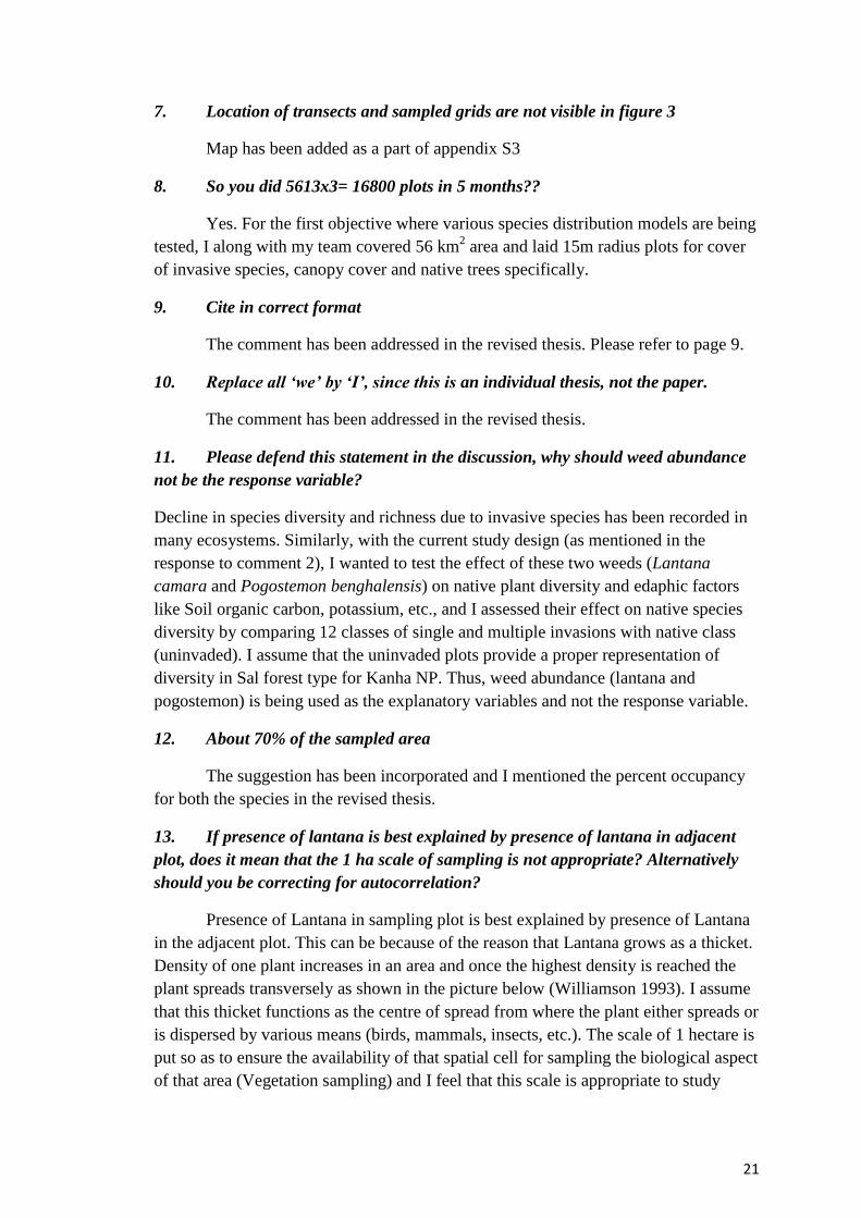
21

7. Location of transects and sampled grids are not visible in figure 3

Map has been added as a part of appendix S3

8. So you did 5613x3= 16800 plots in 5 months??

Yes. For the first objective where various species distribution models are being

tested, I along with my team covered 56 km2 area and laid 15m radius plots for cover

of invasive species, canopy cover and native trees specifically.

9. Cite in correct format

The comment has been addressed in the revised thesis. Please refer to page 9.

10. Replace all ‘we’ by ‘I’, since this is an individual thesis, not the paper.

The comment has been addressed in the revised thesis.

11. Please defend this statement in the discussion, why should weed abundance

not be the response variable?

Decline in species diversity and richness due to invasive species has been recorded in

many ecosystems. Similarly, with the current study design (as mentioned in the

response to comment 2), I wanted to test the effect of these two weeds (Lantana

camara and Pogostemon benghalensis) on native plant diversity and edaphic factors

like Soil organic carbon, potassium, etc., and I assessed their effect on native species

diversity by comparing 12 classes of single and multiple invasions with native class

(uninvaded). I assume that the uninvaded plots provide a proper representation of

diversity in Sal forest type for Kanha NP. Thus, weed abundance (lantana and

pogostemon) is being used as the explanatory variables and not the response variable.

12. About 70% of the sampled area

The suggestion has been incorporated and I mentioned the percent occupancy

for both the species in the revised thesis.

13. If presence of lantana is best explained by presence of lantana in adjacent

plot, does it mean that the 1 ha scale of sampling is not appropriate? Alternatively

should you be correcting for autocorrelation?

Presence of Lantana in sampling plot is best explained by presence of Lantana

in the adjacent plot. This can be because of the reason that Lantana grows as a thicket.

Density of one plant increases in an area and once the highest density is reached the

plant spreads transversely as shown in the picture below (Williamson 1993). I assume

that this thicket functions as the centre of spread from where the plant either spreads or

is dispersed by various means (birds, mammals, insects, etc.). The scale of 1 hectare is

put so as to ensure the availability of that spatial cell for sampling the biological aspect

of that area (Vegetation sampling) and I feel that this scale is appropriate to study

22

distribution of invasive plants. Since percent cover of invasive species in the adjacent

cells is taken into consideration, I corrected for autocorrelation.

14. If this is compared to the naïve estimate of 70% area, esp the BDM model,

how do you explain the small area (approx. 25% ) predicted?

The total study area is 231km2, out of which 56km

2 (24%) area was sampled

for cover of invasive plants. The estimate of 71% of area being invaded by lantana and

66% by pogostemon is based on the surveyed area of 56 km2, whereas, the modelled

distribution is for complete study area.

In the Biophysical density model (BDM), we used the physiological thresholds from

the Biophysical threshold model (BTM) and incorporated densities of both invasive

plants by using Bayesian density kriging. Each Species distribution models being used

were further validated using 25% of the known data cells and checked for sensitivity

and specificity indices. Taking p<0.05 as the validation criterion, If the predicted and

known presences showed an overlap or a difference, they were considered as presence

or absence respectively.

15. Birds are not in the objective

The word 'Bird' has been removed from the revised thesis. Please refer to page

number 25.

16. Use full variable names, and cut down on decimal places

Suggestion has been incorporated in the revised thesis. Please refer to page 30.

17. Can the difference be tested for significance?

I did not test the differences for significance but the means of response

variables (diversity indices and edaphic factors) with standard errors. Also, the

comparison for all the response variables was made between the uninvaded class and

twelve classes of invasion (Table 1). The estimates of their errors is provided in the

appendix S7

18. Are these the results of t-tests? Are the samples independent? Anything will

be significant with a sample size of 5600 or 18000.

23

No, the results are of linear modelling in an ANOVA framework. The detailed

table is given in appendix S7. The samples were independent in an spatial and design

context.

For the second objective the sample size was 120 sampling plots. The sampling was

considered to be completed when for all the vegetation taxa, species asymptotes were

acquired.

19. Do you have estimates of error on the indices?

Yes, the error estimates are given in the appendix S7 with individual tables.

For the ease in reading and understanding, I tried to make these tables coloured, where

green colour signifies highest value decreasing to the colour red. And values which

either decrease or increase significantly (p<0.05) w.r.t. NPNL (uninvaded plots) are

BOLD

20. Can you call 50% less? If there is correlation only after 50% what is the

effect size?

I have corrected my statement here and less is replaced by 'lesser'. It is a

relative connotation to the magnitude of invasion. Also, there have been studies

mentioning about the threshold after which the dignificant effects of invasive species

are found (75% in case of lantana).

21. Please rewrite this paragraph, it is not clear what you are trying to say.

The suggestion has been incorporated in the discussion section (Page 39 and

40).

22. In the light of the fact that this is an observational study, how do you account

for the mechanism of these processes? How do the weeds do this?

I tried to make a theoretical context of the prospective mechanisms which

might be underlying with biological invasions. I observed the increased abundance of

nitrogen and calcium fixing plants when lantana was present in higher abundance.

Which, I feel can be an indication towards the patterns of altered nutrient dynamics,

where, N-C ratios in soil changes leading towards a homogenized community

dominated by few common species. This can be attributed to the theoretical

explanation that invasive plants take in resources from soil and alter with the nutrient

cycling, they are also found to have deleterious impacts on native biodiversity (as

mentioned in the previous answers). These theoretical phenomena have been tested

and affirmed by various studies (Ehrenfield 2001, Ehrenfield 2003).