MARINE ECOLOGY PROGRESS SERIESMar Ecol Prog Ser

Vol. 364: 181–197, 2008doi: 10.3354/meps07499

Published July 29

INTRODUCTION

Several policy commitments to protect marine biodi-versity, both globally and regionally, underpin therecent moves towards an ‘ecosystem approach to man-agement’ (EAM) in the North Sea (Greenstreet 2008).The convention for the protection of the marine envi-ronment of the north-east Atlantic, OSPAR, deemedthe competent authority to develop the EAM, identi-fied 10 key ecological quality issues for the North Seaand requested relevant expert bodies, such as theInternational Council for the Exploration of the Sea(ICES), to define ecological quality objectives (Eco-QOs) for each issue. Developing the EAM along theselines requires indicators that portray the ‘state’ of dif-

ferent components of marine ecosystems (Jennings &Reynolds 2000, Frid 2003, Garcia & Cochrane 2005).

Groundfish surveys, carried out for decades in sup-port of traditional fisheries management, provide dataon the numbers at length of all species sampled(Heessen 1996, Heessen & Daan 1996). Such data areideal for the computation of many multi-species com-munity descriptors (e.g. Washington 1984). Since ‘fishcommunities’ was the fifth in OSPAR’s list of 10 eco-logical quality issues (Johnson 2008, Heslenfeld &Enserink 2008), examining long-term change of differ-ent aspects of the North Sea demersal fish communityreceived considerable attention (Greenstreet & Hall1996, Hall & Greenstreet 1996, 1998, Rice & Gislason1996, Greenstreet et al. 1999, Jennings et al. 1999, 2002,

© Inter-Research 2008 · www.int-res.com*Email: s.greenstreet@marlab.ac.uk

Assessing the sampling effort required to estimateαα species diversity in the groundfish assemblages

of the North Sea

Simon P. R. Greenstreet1,*, Gerjan J. Piet2

1Fisheries Research Services, Marine Laboratory, PO Box 101, Victoria Road, Aberdeen AB11 9DB, UK2Wageningen IMARES, PO Box 68, 1970 AB IJmuiden, The Netherlands

ABSTRACT: Conserving and restoring biodiversity are key objectives for an ecosystem approach tomanagement in the North Sea, but ecological quality objectives for the groundfish communityinstead concentrate on restoring size structure. Species richness and diversity estimates are stronglyinfluenced by sampling effort. Failure to account for this has led to the belief that species richness anddiversity indices are not adequate indicators of ‘state’ for the groundfish community. However, ad-herence to a standard procedure that is robust within respect to sampling effort influence shouldallow these metrics to perform a state indicator role. The Arrhenius power and Gleason semi-log spe-cies–area relationships are examined to determine whether they can provide modelled estimates ofspecies richness at the ICES (International Council for the Exploration of the Sea) rectangle scale. Ofthese, the Gleason semi-log appears most reliable, particularly when a randomised aggregation pro-cess is followed. Aggregation of at least 20 trawl samples is required to provide empirically derivedindex values that are representative of the communities sampled, and therefore sensitive to drivers ofchange in these communities. However, given current groundfish survey sampling levels, combining20 half-hour trawl samples to provide single estimates of species richness and diversity will requireconsiderable aggregation over time and/or space. This can lead to estimates of α or local richness/diversity becoming inflated through the inclusion of elements of β or regional richness/diversity. Forthe North Sea groundfish assemblage, this occurs when the distance between the focal position andthe location of the most distant sample exceeds 49 km.

KEY WORDS: Ecosystem approach to management · State indicators · Sample-size dependency ·Species–area relationships · α-diversity · β-diversity · Management frameworks

Resale or republication not permitted without written consent of the publisher

Mar Ecol Prog Ser 364: 181–197, 2008

Rogers et al. 1999, Rogers & Ellis 2000, Piet & Jennings2005). Long-term declines in species richness anddiversity were revealed (e.g. Greenstreet & Hall 1996,Rijnsdorp et al. 1996, Greenstreet et al. 1999), andshown to be a result of fishing activity (Greenstreet &Rogers 2006). Given the political concern over bio-diversity, one might have anticipated that the EcoQOfor fish communities would address this decline infish species diversity. Instead, the EcoQO is directedtowards restoring the size structure of demersal fish inthe North Sea (ICES 2007, Greenstreet 2008). How didthis change in focus arise?

When asked by OSPAR to recommend appropriatestate indicators to support an EcoQO for Fish Com-munities, ICES proposed 7 criteria on which to basetheir judgement (ICES 2001). These criteria, listed inTable 1, place considerable emphasis on the linkagebetween indicator performance and the anthropogenicactivity in question. Species diversity indices per-formed poorly against several of these criteria, and sowere discarded as possible state indicators for the fishcommunity EcoQO (Greenstreet 2008). Explainingwhy species diversity indices performed so poorly wasthe main purpose of this study. To do this, attentionwas directed towards 3 of the criteria (criteria b, c, andd; Table 1) that proved to be the most serious impedi-ments to using species diversity indices.

Criterion b in Table 1 requires a good state indicatorto be ‘sensitive to a manageable human activity’. Inthe northern North Sea, analysis of Scottish Augustgroundfish survey (SAGFS) data revealed steeperdeclines in groundfish species diversity in areas wherefishing activity levels were highest (Greenstreet & Hall1996, Greenstreet et al. 1999, Greenstreet & Rogers2006), suggesting that species diversity indices were

sensitive to fishing activity. However, other studiesrevealed no, or even positive, trends in species diver-sity, depending on the data set analysed (e.g. Rogers &Ellis 2000, Piet & Jennings 2005). This inconsistencyled ICES (2001) to conclude that diversity indices werenot particularly sensitive to fisheries-related impactson the marine ecosystem (see also Chadwick & Canton1984, Robinson & Sandgren 1984). Most diversity indi-ces are sample-size dependent (Magurran 1988, Col-well et al. 2004). Frequently, problems have arisenthrough failure to appreciate the influence of samplingeffort on index performance. If sampling effort re-quirements are not assessed a priori, the application ofdiversity indices to samples of inadequate size leads toinsensitive metrics that fail to detect real differences indiversity (Soetaert & Heip 1990, Boulinier et al. 1998).

The problem is exemplified by island biogeographytheory, wherein species richness increases as a (Arrhe-nius) power function of the area sampled:

S = cAz (1)

where S is the species richness count, A the area sam-pled, and c and z are constants (MacArthur & Wilson1967, Rosenzweig 1995).

This implies that local (α) species richness (Hill’s[1973] index N0) cannot be determined empiricallywithout sampling the entire habitat area. Instead, bysequentially aggregating samples and tracking boththe total aggregated species richness and the totalaggregated area sampled, the species–area relation-ship (SAR) can be parameterised and used to modelspecies richness in the area in question (e.g. Palmer1988, 1990, Colwell & Coddington 1994, Keating et al.1998, Gotelli & Colwell 2001, Storch et al. 2003, Uglandet al. 2003, Fridley et al. 2005, O’Hara 2005, vanGemerden et al. 2005). Species diversity indices thattake account of relative species abundance are simi-larly influenced by sampling effort. Hill’s (1973) N1 andN2 are, respectively, mathematically defined as:

(2)

where ps is the proportion of the total number of indi-viduals sampled contributed by each of the S speciesrecorded in the sample (Magurran 1988).

The inclusion of additional species with increasingsampling effort increases the number of ps values ineach of the summation terms, thereby affecting bothindices.

Piet & Jennings (2005) computed their richness anddiversity index values as the ‘mean value per haul’ ineach year of the 2 groundfish survey time-series thatthey analysed. However, as illustrated above, speciesrichness of the community will always be higher than

N e and Nln

1 22

1

1 1= =− ∑

=

=

∑* ( )p p

ss

Ss

s

S

s

p

182

Criterion Property

a Relatively easy to understand by non-scien-tists and those who will decide on their use

b Sensitive to a manageable human activityc Relatively tightly linked in time to that activityd Easily and accurately measured, with a low

error ratee Responsive primarly to a human activity, with

low responsiveness to other causes of change

f Measureable over a large proportion of thearea to which the EcoQ metric is to apply

g Based on an existing body or time-series ofdata to allow a realistic setting of objectives

Table 1. Traffic light system showing results of the applicationof the ICES criteria for a ‘good state indicator’ to speciesdiversity indices (after ICES 2001). Green indicates noappreciable concerns; amber indicates some concerns; red

indicates serious concerns

Greenstreet & Piet: Species diversity in demersal fish

the number of species in any single sample (e.g. Broseet al. 2003). Calculating the mean species richness persample still only provides an estimate of the averagespecies richness in the average area covered in eachsample, and therefore remains a poor indicator of theactual species richness of the community (e.g. Colwellet al. 2004). Reporting species richness as richness perunit sampling effort is theoretically unsound because,as indicated by the SAR, species richness (S) is propor-tional to Az, and not just to A alone (Rosenzweig 1995).Since z is a parameter that is characteristic of eachcommunity sampled, in each case, it is a parameterthat needs to be estimated.

Application of the traditional Arrhenius power func-tion assumes that local species assemblages are simplysub-sets of the regional species pool (Cornell & Lawton1992, Angermeier & Winston 1998, Cornell & Karlson1997, Findley & Findley 2001). However, studies exam-ining the role of regional and local processes in dictat-ing local species richness have demonstrated a phe-nomenon termed ‘saturation’. After an initial sharp riseas the first samples are aggregated, the species accu-mulation rate drops markedly compared with the ever-increasing traditional Arrhenius power function (Find-ley & Findley 2001, Cottenie et al. 2003, Heino et al.2003, Kiflawi et al. 2003, Wright et al. 2003). This hasled to debate over which function best fits the SAR.There may be a fundamental difference between local-and regional-scale SARs; the latter may be best fittedby the Arrhenius power function, while the former arebest fitted by the Gleason semi-log plot, S = c + z(logA)(Whittaker 1972, van der Maarel 1988, Stohlgren etal. 1995). At local spatial scales, extrapolation from atraditional Arrhenius power function SAR could over-estimate species richness in specified areas, such asICES 0.5° latitude by 1° longitude statistical rectangles(Fridley et al. 2005).

Neither the Gleason nor the Arrhenius model isasymptotic in nature; both imply that additional sam-pling will always reveal new species. Species satura-tion could suggest that an asymptotic model, such asthe Michaelis-Menton equation, might be more suit-able to estimate local (α) diversity (e.g. Soberón &Llorente 1993, Denslow 1995, Keating & Quinn 1998).However, asymptotic models are only appropriatewhen the local habitat is absolutely defined (e.g. amountain slope, Denslow 1995) and sampling isexhaustive (Magurran 2004). ICES statistical rectan-gles are arbitrarily defined and cover an area ofapproximately 3640 km2. The average groundfish sur-vey rarely includes more than 4 trawl samples per rec-tangle, each covering an area of 0.07 km2, so samplingis not exhaustive. Asymptotic models therefore do notprovide appropriate SARs to estimate ICES rectangle-scale species richness.

The sample aggregation method may also influencethe resultant SAR. Several authors (e.g. Rosenzweig1995, Fridley et al. 2005) have suggested that samplesbe nested (each new area sampled is contiguous withthe area sampled in samples lower in the aggregationorder). In randomised aggregation, samples adjacentin the aggregation order may be separated in space,increasing the probability that the new sample willinclude new habitats, and hence add new species morequickly. Nested aggregation, focusing on α-diversity,produces shallower species accumulation curves(Palmer 1990, Rosenzweig 1995), while a randomisedapproach may more rapidly incorporate elements ofβ-diversity (Colwell et al. 2004). The type of aggrega-tion could have an influence on which SAR best fits thedata: nested aggregation may be better fitted by theArrhenius power function, while the Gleason semi-logplot may provide a better fit to randomised aggrega-tions.

An alternative approach is to estimate the samplesize required to derive indices of species richness andspecies diversity that reflect actual rankings in speciesrichness and diversity in sampled communities. Thismay not provide estimates of actual species richnessand diversity, but should allow temporal or spatialtrends to be detected. This approach was adopted inthe SAGFS studies discussed above. Preliminaryanalysis revealed that 10 h of Aberdeen 48-foot ottertrawl effort was necessary before the aggregated sam-ple obtained produced reliable estimates of Hill’s N0,N1 and N2 (Greenstreet & Hall 1996, Greenstreet et al.1999, Greenstreet & Rogers 2006). Accounting for sam-ple-size dependency in this way provided indices sen-sitive enough to detect long-term, fishing-relateddeclines in demersal fish species richness and diversityin the northwestern North Sea.

This approach, however, also has drawbacks.Marine sampling is difficult and expensive, limitingthe level of sampling effort that is feasible. The bestsupported North Sea groundfish surveys, the ICES first(Q1) and third quarter (Q3) International Bottom TrawlSurvey (IBTS), rarely achieve more than 3 trawl sam-ples per ICES rectangle surveyed per year. Addressingspatial questions will therefore require the aggrega-tion of samples collected over several years; con-versely, investigating temporal issues will require theaggregation of samples collected across several ICESrectangles (e.g. Greenstreet & Rogers 2006). Moststudies will be directed towards estimating α-diversity;the diversity in a particular location (habitat, ICES rec-tangle, etc.) at a given point in time. Aggregationacross space risks including new species as new habi-tats get included in the aggregated sample area, thusconfounding α-diversity with β-diversity (Whittaker1972, Lande 1996, Kiflawi & Spencer 2004). Similarly,

183

Mar Ecol Prog Ser 364: 181–197, 2008

temporal turnover of vagrant species may lead to over-estimation of species richness when samples areaggregated over time (Hadley & Maurer 2001, Adler &Lauenroth 2003, Adler et al. 2005, White et al. 2006,Magurran 2007, Shurin 2007). Both processes wouldtherefore tend to inflate estimates of α-species rich-ness.

The lack of a consistent approach to estimating spe-cies diversity and species richness from groundfishspecies abundance data has produced inconsistentresults. In the past, studies that took account of sam-ple size dependency showed significant trends anddemonstrated fishing effects, while studies that ig-nored sample size dependency produced results thatwere difficult to interpret. This inconsistency led ICES(2001) to conclude that metrics of species diversityand richness were either insensitive to a manageablehuman activity, or not tightly linked to the activity,illustrating that the use of diversity indices is notstraightforward. Depending on how they are deter-mined, indices of species richness and species diversitymay not be easily and accurately measured. In a morerecent treatise on the characteristics desirable in astate indicator, the capacity to convey information onaspects of the ecosystem that are of societal concernwas assigned high priority (Rice & Rochet 2005). Con-serving and restoring biodiversity remain key principalpolicy drivers underlying the implementation of anEAM, which underlines the need for operational bio-diversity state indicators. Addressing the problemsidentified by the application of the ICES criteria to bio-diversity metrics is therefore an urgent priority formarine scientists.

A systematic approach to applying species diversityand richness metrics to groundfish survey data shouldrectify many of these problems, enabling such metricsto perform the role of state indicators and allowing theconservation and restoration of biodiversity to beaddressed directly. Therefore, this study examines thesample size dependency of Hill’s (1973) indices ofspecies richness and diversity (N0, N1 and N2) in orderto establish a standard procedure for their use. Todemonstrate such a procedure, the question of map-ping groundfish species richness and diversity acrossthe North Sea is addressed. First, spatial variation inspecies composition is examined to ensure that, whenselecting samples for sequential aggregation to ex-plore the effect of sampling effort on metric perfor-mance, samples are drawn from similar species assem-blages. Six such sites are selected covering a widegeographic area and 3 different assemblages. Havingestablished a suitable procedure to estimate speciesrichness and diversity in each ICES rectangle, spatialvariation in the 3 Hill’s metrics is determined by aggre-gating the necessary number of samples closest to the

centre point of all rectangles included in the survey.The extent to which this spatial aggregation results inconfounding elements of β-diversity into each of theindividual ICES rectangle estimates of α-diversity isthen explored, and the impact this has on qualitativeassessment of the resulting diversity maps is exam-ined.

METHODS

The Q3 IBTS survey effort is approximately evenlydistributed over ICES statistical rectangles across thewhole North Sea. Each rectangle is usually fished byships belonging to 2 participating countries using agrande ouverture verticale (GOV) trawl, resulting in atleast 2 hauls per rectangle in most rectangles in mostyears. Numbers at length of all species caught aredetermined, and information on location, distancetowed, and area swept by the gear is noted. Followingprevious practice (e.g. Greenstreet & Hall 1996,Greenstreet et al. 1999), only data for species consid-ered to be members of the ‘demersal fish community’were analysed. Prior to 1998, not all participatingcountries used the same trawl gear, and tow durationsvaried. After 1998 all participating countries used theGOV trawl gear and tow duration was standardised to30 min across the entire survey. Therefore, only datacovering the period 1998 to 2004 were analysed. Thisproduced the most consistent data set in terms of sam-pling procedure on which to base analyses of speciesdiversity.

Data for a total of 2076 hauls were available. Despitefairly rigid protocols being laid down for the IBTS,these trawl samples varied markedly in terms of theirswept area. Because of the sensitivity of diversity met-rics to variation in sampling effort, ‘valid’ trawl sam-ples were defined on the basis of swept area (Fraser etal. 2008), and only trawl samples conforming to thisstandard were analysed. This process resulted inapproximately 8% of the IBTS trawl samples beingexcluded, leaving 1909 trawl samples with swept areasranging from 51 473 to 80 835 m2 available for analysis.

Similarity in the species composition of the demersalfish community sampled in different ICES rectangleswas assessed using the Bray-Curtis similarity index.Data for all trawl samples in each ICES rectangle werecombined to provide a single species abundance ‘sam-ple’. Abundance data were root-root transformed todown-weight the effects of the more abundant species.Similarity between all pairs of ICES rectangles wasdetermined. The resulting similarity matrix was sub-jected to hierarchical group-average cluster analysis toidentify groups of ICES rectangles with demersal fishcommunities of similar species composition. These

184

Greenstreet & Piet: Species diversity in demersal fish

analyses were performed using the PRIMER software(Clarke & Warwick 2001). Six ICES rectangles werechosen for detailed analysis of the influence of sam-pling effort on the performance of 3 species diversityindices. Criteria for selection were:

• the focal rectangles should be widely dispersedacross the North Sea

• the focal rectangles should belong to at least 3different species composition groups

• the number of trawls in the focal rectangles shouldbe relatively high

• all rectangles adjacent to the focal rectanglesshould belong to the same species composition group.

There are 2 different aspects to species diversity: theactual number of species included in any particularsample, and the evenness of the distribution of individ-uals between all species encountered. Three metricscommonly used in analyses of groundfish survey datawere applied (e.g. Greenstreet & Hall 1996, Green-street et al. 1999, Piet & Jennings 2005), each differingin the extent to which they are influenced by theseaspects of species diversity (Southwood 1978). Hill’s N0

is simply the count of all species (species richness)encountered in a sample, a metric strongly influencedby sampling effort variation. Two indices of speciesdiversity (Hill’s N1 and N2, the exponential of the Shan-non-Weiner index and the reciprocal of Simpson’sindex, respectively) were also applied. The mathemat-ical notation for both N1 and N2 is provided in Eq. (2).N1 is more sensitive to variation in the number of spe-cies recorded in a sample, whereas N2 is more sensi-tive to variation in the evenness of the distribution ofindividuals between species. All diversity metrics weredetermined using PRIMER (Clarke & Warwick 2001).

At least 91 trawl samples (across all 7 years) wereavailable for analysis in each of the 6 focal rectanglesand their immediate neighbours. To apply the rando-mised aggregation method, 90 samples were selectedat random (without replacement) from the availablesample pool and sequentially aggregated. After theaddition of each new sample, the total area swept byall aggregated samples was determined and the valueof each of the 3 metrics calculated on the combinedspecies abundance data. The order in which samplesare aggregated affects the shape of the SAR, depend-ing on whether the first sample in the accumulationorder happens to be relatively species rich or speciespoor, compared with the remaining samples (Palmer1990). To counter this, the sequential sample aggrega-tion process was repeated 10 times, so that the order ofaggregation was also randomised. Arrhenius powerand Gleason semi-log functions were fitted to the datafor all 10 randomisations. A true nested aggregationcould not be carried out, because the IBTS trawl sam-ples were not adjacent to each other in space. Such

sampling has never been a survey requirement. How-ever, as an approximation to this approach, 90 sampleswere aggregated in order of their distance from thecentre-point of each of the 6 focal rectangles. Only oneaggregation order fitted this criterion, so no replicationwas possible. Again, both the Arrhenius power andGleason semi-log functions were fitted to the resultingaccumulation curves.

As samples were aggregated to estimate ICES rec-tangle-scale index values for each of Hill’s metrics, theactual extent of the area from which these sampleswere obtained also increased. Variation in the areafrom which the samples were collected was measuredusing a metric termed the ‘search radius’. This wasdefined as the distance from the sample focal point(e.g. the centre position of an ICES rectangle) and thelocation of the most distant sample in the sampleaggregation.

RESULTS

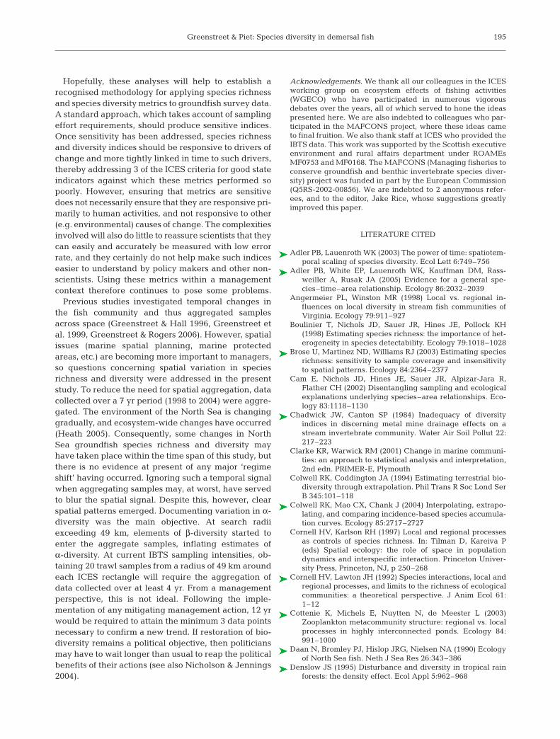
Cluster analysis of the ICES rectangle species abun-dance data revealed distinct groups of rectangles withsimilar species composition. When these clusters weremapped, clear spatial organisation was apparent(Fig. 1). On the basis of the data shown in Fig. 1 and thecriteria given above, 6 ICES rectangles (‘assemblages’)were selected for investigation of the effect of samplingeffort on species diversity index performance.

Randomised aggregations

In 5 of the 6 assemblages (the exception being Red2),the R2 values obtained (Table 2) suggested that speciesrichness (Hill’s N0) was best fitted by the Gleason semi-log function, rather than by the Arrhenius power func-tion (Fig. 2). Residuals to the Arrhenius power functionshowed a significant negative departure from theexpected distribution at high sample aggregation lev-els (large A) in 4 (Red1, Green1, Green2 and Pink1) ofthe 6 rectangles (Fig. 2). Consequently, estimates ofICES statistical rectangle-scale (3642 km2 in the cen-tral North Sea) species richness based on extrapolationof the fitted Arrhenius power functions were unrealis-tically high (Table 2). The total North Sea fish speciesinventory, including pelagic species excluded from thisanalysis, has been estimated at around 224 species(Yang 1982). Extrapolation of the Gleason semi-logfunctions provided more reasonable estimates of rect-angle-scale species richness (Table 2). However, re-siduals to the Gleason semi-log function showed asignificant positive departure from the expected dis-tribution at high sample aggregation levels in the other

185

Mar Ecol Prog Ser 364: 181–197, 2008

2 assemblages, Red2 and Pink2 (Fig. 2), suggestingthat, in these cases, the Gleason semi-log functionmight under-estimate ICES rectangle-scale speciesrichness. In summary, 5 of the assemblages (Red1,Green1, Green2, Pink1 and Pink2) were better fittedby the Gleason semi-log function, but with Pink2,showing significant positive deviations from the fit athigh sample aggregation levels, and 1 assemblage,Red2, was best fitted by the Arrhenius power function.

The Arrhenius and Gleason functions produced asimilar, but not identical, ranking of the 6 assemblagesin terms of their ICES rectangle-scale species richness(Table 2). The Arrhenius power function ranked theassemblages Pink1 > Green1 > Red1 > Green2 > Pink2> Red2, while the Gleason semi-log function inter-changed the first and second, and third and fourthrectangles to rank the assemblages Green1 > Pink1 >Green2 > Red1 > Pink2 > Red2. However, 95% confi-dence limits (CLs) around the ICES rectangle-scaleestimates of species richness of both the interchangedassemblage pairs overlapped, regardless of the SARapplied to the data (Table 2). Neither of the SARs couldtherefore provide a definitive ranking order for these 2

assemblage pairs. Given that the Gleason semi-logfunction provided the best fit to the data from the 4 top-ranked assemblages, the latter ranking is probably themost reliable. Even though the Gleason semi-logfunction probably underestimated species richness inthe 2 lowest-ranked assemblages, these same 2 assem-blages were also ranked lowest, and in the same order,by the Arrhenius power function.

More critically, the assemblage rankings were notestablished until both SARs had been extrapolated toareas greater than 40 km2. At aggregation levels of 90trawl samples, the total area sampled was approxi-mately 7 km2 (Fig. 3), suggesting that the samplingrequired to rank fish communities using empirical esti-mates of ICES rectangle-scale groundfish species rich-ness (i.e. based simply on aggregated sample speciescounts) would be too onerous and well beyond current,or likely, levels of groundfish survey activity. However,the situation is not as stark as this initial assessmentsuggests. Deciding relative species richness rankingsbetween the Red1 and Green2 and between the Pink1and Green1 assemblages posed the greatest difficultywhen using the Arrhenius power function (Fig. 3).

186

66

87

7157

1353

711161712179

177745

12131313161924199

18141210114

3131213111316171219201513131313156

12

6121514131315161321131214121412125

126

135

13131213141416131213171411171213

115

127

13191318141315131213151611124

4116

14191421131414151112

141914201413141413

720141913141651

3413201415125

1

Longitude

50°4° 2° 0 2° 4° 6° 8° 10°W E

51°

52°

53°

54°

55°

56°

57°

58°

59°

60°

61°

62°

63°N

ba

100 80 60 40

Latit

ude

Similarity ≥≥ 70%

Similarity ≥≥ 65%

Bray-Curtis similarity (%)

Pink 1

Pink 2

Red 1

Red 2

Green 1

Green 2

Fig. 1. (a) Results of hierarchical group-averaging cluster analysis of the Bray-Curtis similarity matrix constructed for the Interna-tional Bottom Trawl Survey (IBTS) grande ouverture verticale (GOV) data set. Clusters of ICES rectangles grouped at similaritylevels of 65 and 70% are colour coded. (b) Chart of spatial distribution of groups from (a). The chart indicates the number of GOVtrawl samples available for analysis in each ICES rectangle over the full period 1998 to 2004. The 6 focal rectangles (assemblages)

selected for ‘sample-size’ analyses are annotated

Greenstreet & Piet: Species diversity in demersal fish

Similarly, defining the ranking order of the Pink1 andGreen2 assemblages was hardest when using theGleason semi-log function (Fig. 3). For clarity, 95%CLs were not shown in Fig. 3, but reference to Table 2reveals that the 95% CLs around the species richnessestimates of each assemblage within these assemblagepairs overlap. Within each pair, the assemblage rank-ing order could not therefore be conclusively defined,and if this is the case, Fig. 3 suggests that extrapolationof the SARs to an area of 7 km2 was sufficient to pro-vide relative species richness rankings. Estimates ofspecies richness capable of ranking the species rich-ness of different ICES rectangle groundfish assem-blages might therefore be empirically derived fromaggregated collections of 90 half-hour GOV trawlsamples.

The sample aggregation–species diversity plots forthe 2 species diversity indices, Hill’s N1 and N2,

revealed horizontal, funnel-shapedforms that differed markedly from thespecies richness (Hill’s N0) ‘dataclouds’ (Fig. 2). This is because N1 andN2 take account of both aspects ofdiversity, species richness and speciesevenness. With species richness, it ispossible that the first sample in theaccumulation order might be par-ticularly species rich or particularlyspecies poor, thereby causing theobserved spread of data at the left ofthe data clouds (Fig. 2). However, it isalso inevitable that, as the combinedarea sampled increases, new specieswill be added to the aggregated total,no matter how high the initial startpoint. Stochastic variation in the spe-cies richness of the first samplesaggregated also affects N1 and N2 in asimilar fashion, causing the generallypositive convex shape of the dataclouds in many of the plots (Fig. 2).However, the degree of evenness alsovaries in a stochastic manner, so thatthe first samples in an aggregationorder might be characterized by rela-tively low levels of dominance (un-usually low abundance of normallydominant species, or higher-than-usualabundance of some less common spe-cies), resulting in unusually high N1

and N2 values. Further accumulationof additional samples characterized bymore normal levels of dominance thencauses aggregated N1 and N2 valuesto fall. This gives rise to the character-

istic funnel-shaped data clouds prevalent in Fig. 2.Since neither of the SARs can be consistently fitted toeither of the diversity indices, a similar statisticalmodel-fitting approach to estimating species diversityat the ICES rectangle spatial scale was not possible.However, once the total aggregated area sampled wassufficiently large, the data tended to stabilize aroundmean index values. Therefore, the mean index value,calculated across all 10 randomised aggregations of 90samples, probably provides the most reliable estimateof species diversity at the ICES rectangle scale for eachof the 6 assemblages (Table 3).

Nested aggregations

Arrhenius power functions provided marginallyhigher R2 values for 4 (Red1, Green2, Pink1 and Pink2)

187

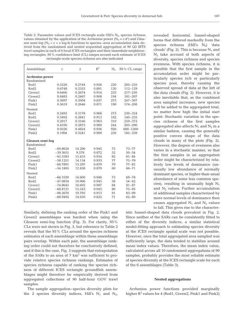
Assemblage c z R2 N0 95% CL range

Arrhenius power RandomisedRed1 0.5226 0.2744 0.926 220 205–235Red2 0.6748 0.2353 0.891 120 112–129Green1 0.6466 0.2674 0.914 233 217–250Green2 0.8483 0.2467 0.908 194 181–207Pink1 0.3697 0.3004 0.857 275 247–307Pink2 0.5619 0.2646 0.871 190 174–208

NestedRed1 0.2493 0.3179 0.968 273 230–324Red2 0.3492 0.2841 0.913 182 140–235Green1 0.2917 0.3166 0.963 310 259–372Green2 0.4356 0.2875 0.960 244 205–290Pink1 0.0226 0.4824 0.956 926 680–1260Pink2 0.1994 0.3241 0.909 250 185–339

Gleason semi-logRandomisedRed1 –60.8624 14.206 0.945 75 73–77Red2 –39.3651 9.578 0.872 52 50–54Green1 –65.3583 15.455 0.954 82 81–84Green2 –58.1251 14.154 0.933 77 75–79Pink1 –66.7891 15.297 0.879 79 77–82Pink2 –54.1805 12.838 0.879 69 66–71

NestedRed1 –66.1030 14.600 0.946 73 69–78Red2 –47.0834 10.966 0.945 58 54–62Green1 –74.8645 16.602 0.987 84 81–87Green2 –68.8151 15.543 0.945 80 75–85Pink1 –98.2670 19.795 0.913 91 83–99Pink2 –68.9492 14.650 0.825 71 62–80

Table 2. Parameter values and ICES rectangle scale Hill’s N0, species richnessvalues obtained by the application of the Arrhenius power (N0 = cAz) and Glea-son semi-log (N0 = c + z logA) functions to species–area accumulation data de-rived from the randomised and nested sequential aggregation of 90 Q3 IBTStrawl samples in each of 6 focal ICES rectangles and their immediate neighbour-ing rectangles. 95% confidence limit (CL) ranges around each estimate of ICES

rectangle-scale species richness are also indicated

Mar Ecol Prog Ser 364: 181–197, 2008

of the 6 assemblages species richness plots (Fig. 4), butin all cases extrapolation to the area of an ICES rect-angle again resulted in unrealistically high estimatesof species richness (Table 2). Gleason semi-log func-tions may not have fitted the data quite so well, but the

differences were small, and extrapolation to the ICESrectangle scale resulted in more reasonable estimatesof species richness (Table 2). The Arrhenius functionranked the 6 assemblages Pink1 > Green1 > Red1 >Pink2 > Green2 > Red2, while the Gleason function

188

0

10

20

30

40

50N

0N

1N

2Green 2Green 1Red 2Red 1 Pink 1 Pink 2

0

1

2

3

4

5

6

7

0

0 4 8 0 4 8 0 4 8 0 4 8 0 4 8 0 4 8

1

2

3

4

5

6

Area trawled (km2)

Fig. 2. Effect of increasing area sampled on Hill’s N0 (species richness), N1, and N2 (species diversity) index values for each ofthe 6 assemblages, using a randomised sequential aggregation of 90 samples. Data for 10 separate randomised aggregations areplotted. For N0, solid grey lines show Arrhenius power function fits to the data; dashed grey lines show Gleason semi-log fits

to the data

0

20

40

60

80

No.

of s

pec

ies

Red1Red2Green1Green2Pink1Pink2

Area (km2)

00 10 20 30 40 50

Area (km2)

0 10 20 30 40 50

10

20

30

40

50

60Arrhenius power function Gleason semi-log function

Fig. 3. Extrapolation of the Arrhenius power and Gleason semi-log functions up to 50 km2, illustrating overlaps in each type ofspecies–area relationship (SAR) fitted to the 6 assemblages. Final rankings are not established until extrapolation to areas

greater than 40 km2

Greenstreet & Piet: Species diversity in demersal fish

ranked them Pink1 > Green1 > Green2 > Red1 >Pink2 > Red2, elevating the fifth ranked assemblageinto third place. In both cases, the 95% CLs around theICES rectangle-scale species richness estimates for theassemblages ranked 3, 4 and 5 overlapped, so neitherSAR could conclusively rank these 3 assemblages. Foreach SAR, the aggregation method had little effecton the assemblage rankings. Compared with the ran-domised aggregation, nested aggregations transposedthe fourth- and fifth-ranked assemblages using theArrhenius function, whilst the first and second assem-

blages were transposed when the Gleason functionwas used. In both cases, the 95% CLs around the ICESrectangle-scale species richness estimates for theassemblages concerned again overlapped. A Spear-man rank correlation matrix, comparing the 4 sets ofspecies richness estimates, confirmed the similarity inranking order achieved by all 4 methods (Table 4), butno 2 ranking orders were identical.

Nested aggregation plots for Hill’s N1 and N2 speciesdiversity indices revealed a variety of forms (Fig. 4),demonstrating the interplay between species richnessand species evenness in influencing index behaviourwith increasing sampling effort. Index values sta-bilised to some extent, once the aggregated samplearea exceeded 1 to 2 km2. However, compared withthe randomised aggregation plots (Fig. 2), even in thefinal stages of aggregation, clear positive or negativetrends in both indices were still apparent for several ofthe assemblages, making it difficult to determineappropriate index values.

The nested aggregation plots for all 3 of Hill’s indiceswere not smooth (Fig. 4), suggesting the influence ofprocesses other than simply the effect of increasing thearea sampled. Fig. 5 shows similar plots, but here theindex values are plotted against search radius (the dis-

189

0

10

20

30

40

50

N0

N1

N2

Green2Green1Red2Red1 Pink1 Pink2

01234567

0

0 4 8 0 4 8 0 4 8 0 4 8 0 4 8 0 4 8

1

2

3

4

5

6

Area trawled (km2)

Fig. 4. Effect of increasing the area sampled (km2) on Hill’s N0 (species richness), N1, and N2 (species diversity) index values ineach of the 6 assemblages, using a nested sequential aggregation of 90 samples. For N0, solid grey lines show Arrhenius power

function fits to the data; dashed grey lines show Gleason semi-log fits to the data

Assemblage N0 N1 N2

Red1 36 3.99 3.14Red2 27 4.94 4.26Green1 40 3.19 2.63Green2 39 2.59 2.07Pink1 37 3.89 3.07Pink2 34 2.83 2.12

Table 3. Average Hill’s N0 (species richness), N1, and N2

(species diversity) index values, calculated across 10 ran-domised aggregations of 90 trawl samples for 6 North Sea

groundfish assemblages

Mar Ecol Prog Ser 364: 181–197, 2008

tance between each new sample in the aggregationand the centre of the ICES rectangle concerned). Fifth-order polynomial functions fitted to these data indi-cated multi-phasic species accumulation curves withmarked increases in the species accumulation rate atsearch distances of around 40 to 50 km. This wasalmost certainly associated with the incorporation ofelements of β-diversity into the estimate of speciesrichness as the region within the expanding searchradius included new habitats with different speciescomposition.

Assessing sample size requirementsfor assemblage ranking

For each of the 6 assemblages, theaverage index value across each of the10 randomised aggregations of 90trawl samples provided the bestempirical estimates of each metric foreach assemblage (Table 3). Thisranked the 6 assemblages, in terms ofspecies richness (Hill’s N0), Green1 >Green2 > Pink1 > Red1 > Pink2 >Red2. Similar to the ranking derivedfrom extrapolation of the randomised

aggregation Gleason semi-log SARs to the ICES rec-tangle scale, just the second and third ranked assem-blages were transposed. This confirms the point madeabove and illustrated in Fig. 3. Even after aggregating90 trawl samples, the ranking of empirical estimates ofspecies richness, based on aggregated sample speciescounts, did not exactly match the ranking obtainedby extrapolating Gleason semi-log SARs to the ICESrectangle scale. Hill’s N1 and N2 both ranked the 6assemblages in identical order: Red2 > Red1 > Pink1 >Green1 > Pink2 > Green2.

190

0

10

20

30

40

50

N0

N1

N2

Green2Green1Red2Red1 Pink1 Pink2

01234567

0

0 40 80 0 40 80 0 40 80 0 40 80 0 40 80 0 40 80

1

2

3

4

5

6

Search radius (km)Fig. 5. Effect of increasing search radius (km) on Hill’s N0 (species richness), N1, and N2 (species diversity) index values in each ofthe 6 assemblages using a nested sequential aggregation of 90 samples. Fitted curves are assemblages fifth-order polynomials

Aggregation Randomised NestedFunction Arrhenius Gleason Arrhenius Gleason

Randomised Arrhenius 0.866 0.943 0.943Gleason p < 0.05 0.771 0.943

Nested Arrhenius p < 0.01 p = n.s. 0.829Gleason p < 0.01 p < 0.01 p < 0.05

Table 4. Spearman correlation coefficients (upper right cells), comparing theranking order of 6 groundfish assemblages in terms of the species richnessdetermined by extrapolation of Arrhenius power or Gleason semi-log functions,fitted to randomised or nested aggregated sample data up to the spatial scaleof the ICES rectangle. Significance levels are indicated (lower left cells;

n.s.: p > 0.05)

Greenstreet & Piet: Species diversity in demersal fish

Next, the level of sample aggregation required inorder to have a good chance of ranking the assem-blages in the correct order was assessed using Pear-son’s correlation. Values determined for each metric ateach aggregation level (as y variables) were comparedwith the mean values obtained for each metric when90 trawls samples were aggregated (as x variables; i.e.Table 3). Correlation coefficients approaching 1 indi-cated good performance, while scores near zero indi-cated poor performance. Negative coefficients implieda reversal of the correct ranking order. Since 10 ran-domisations were carried out, means and standarddeviations of the correlation coefficient at each aggre-gation level could be determined (Fig. 6). For each ofthe 3 metrics, aggregation of at least 20 trawl sampleswas required. By this point, mean Pearson’s R wasclose to the curve asymptotes (>0.75 in all cases), andthe standard deviations around these mean values haddeclined by more than 66%. This does not mean thatestimates of species richness based on 20 GOV trawlsamples indicate actual species richness in any givenICES rectangle. Rather, it suggests that measures ofspecies richness based on 20 or more samples are suf-ficient to compare species richness between differentlocations or different times.

Mapping species richness and species diversity

Hill’s N0, N1 and N2 indices for each ICES statisticalrectangle were derived from the aggregation of the 20trawl samples closest to each rectangles’ central pointand maps of spatial variation of species richness and

diversity were plotted (Fig. 7). Species composition ofthe North Sea groundfish community varied signifi-cantly across space; the greater the distance between 2ICES rectangles, the more different the communities ateach location were (Fig. 8). This confirmed the possi-bility that aggregating samples in space posed a realrisk of confounding β-diversity with α-diversity, lead-ing to inflated estimates of the latter. Consequently, inmapping the 3 indices (Fig. 7), ICES rectangles requir-ing a search radius of >95 km in order to aggregate 20samples were excluded. Relationships between searchradius and each metric were then examined to ensurethat this precaution was sufficient to preclude theincorporation of β-diversity.

Since all metric values were based on identical sam-ple size, there was no reason to anticipate that the met-ric values should be influenced by the search radius.However, this assumption was falsified with respect toHill’s N0, the species richness index (Fig. 9). Below asearch radius of 49 km, N0 was independent of searchradius, but above this distance, N0 was significantlylinearly related to search radius, suggesting increasinginclusion of β-diversity. For all rectangles where thesearch radius required to ‘capture’ 20 trawl samplesexceeded 49 km, this linear regression was used toestimate the β diversity contribution (N0,β) where N0,β =N̂0,SR = x – N̂0,SR = 49. N̂0,SR = x and N̂0,SR = 49 are the esti-mates of N0 obtained from the regression equation atthe observed search radius for each of the rectanglesconcerned and at a search radius of 49 km, respec-tively. This estimated β-diversity contribution was thensubtracted from actual observed estimates of N0 ineach rectangle for which the search radius exceeded

191

No. of hauls

–0.4

0 20 40 60 80 100 0 20 40 60 80 100 0 20 40 60 80 100

–0.2

0

0.2

0.4

0.6

0.8

1

Pea

rson

’s R

N0 N1 N2

Fig. 6. Mean (±1 SD) Pearson correlation scores for different sample aggregation levels of Hill’s N0, N1, and N2 diversity metrics

Mar Ecol Prog Ser 364: 181–197, 2008

49 km. Spatial variation in species richness (N0) acrossthe North Sea was then re-mapped (Fig. 10). Little dif-ference was apparent between this revised map andthe original map (Fig. 7), suggesting that the incorpo-ration of elements of β-diversity in some instances hadlittle effect on qualitative interpretation of spatial vari-ation in α-diversity across the North Sea.

DISCUSSION

The current EcoQO for fish communities in the NorthSea concentrates on the restoration of community sizestructure because fish size metrics were believed tocomply with the ICES criteria for good state indicators(ICES 2007). Indices of biodiversity, on the other hand,were considered to violate too many of these criteria tobe of use within a management context. Conflictingand inconsistent results in studies undertaken in theNorth Sea implied that indices of species richness andspecies diversity were not sensitive to a manageablehuman activity, not responsive primarily to that humanactivity, not tightly linked in time to that activity, or noteasily and accurately measured. Hill’s N0, N1 and N2,the indices of species richness and species diversitymost commonly applied to North Sea groundfish sur-vey data, are shown here to be strongly influenced byvariation in sampling effort. When the influence ofsampling effort has been taken into account by a prioriassessing and then meeting sampling effort require-ments, these indices were sensitive to drivers ofchange in a community (e.g. Greenstreet & Rogers2006). However, when the influence of sampling effortwas ignored, results were less conclusive (e.g. Piet &Jennings 2005). Failure to follow a standard methodol-ogy in applying Hill’s diversity indices to groundfishsurvey data, rather than any failing in the indicesthemselves, may largely be responsible for giving theimpression that these metrics are insensitive to driversof change in the North Sea groundfish community.

192

50°5°W 5°W 5°W0 5° 10°E 10°E 10°E0 5° 0 5°

52°

54°

56°

58°

60°

62°N

Latit

ude

14

18

22

26

30

34

38

14

18

22

26

30

34

38N0

Longitude

1

1.51.5

2

2.52.5

3

3.53.5

4

4.54.5

5

5.55.5

6

1

1.5

2

2.5

3

3.5

4

4.5

5

5.5

6

1

1.1.4

1.1.8

2.2.2

2.2.6

3

3.3.4

3.3.8

4.4.2

4.4.6

1

1.4

1.8

2.2

2.6

3

3.4

3.8

4.2

4.6N1 N2

Fig. 7. Spatial variation in Hill’s N0, N1 and N2 across the North Sea, based on aggregation of the 20 Q3 IBTS trawls closest to thecentral point of each ICES statistical rectangle. Interpolation is by radial basis function in SURFER

Distance between rectangles (km)

00 400 800 1200

20

40

60

80

100

Bra

y-C

urtis

sim

ilarit

y (%

)

BCS = –0.0587D + 79.784N = 11476

R2 = 0.562, p < 0.001

Fig. 8. Relationship between the Euclidean distance betweenpairs of ICES rectangles and the Bray-Curtis similarity (BCS)in species composition of the groundfish community present

in each rectangle

Greenstreet & Piet: Species diversity in demersal fish

Furthermore, because Hill’s metrics were not believedto be sensitive to a human activity, they were also defacto considered not to be tightly linked in time, or to

respond primarily to that activity. Methodological fail-ures in the application of diversity indices have there-fore blighted them across several of the ICES criteria.Consequently, in the minds of many marine scientiststhis precluded the use of diversity indices as state indi-cators, despite the importance of biodiversity as one ofthe principal drivers at the heart of the EAM.

In this study, data from the Q3 IBTS were analysed.This is an international survey coordinated throughICES and supported by many countries within andbeyond the European Union, particularly those with afisheries interest in the North Sea. These surveys haveoperated over at least 2 decades (Heessen 1996,Heessen & Daan 1996, Piet & Jennings 2005), andbecause of their importance to the traditional stockassessment process (ICES 2006), they will no doubtcontinue to provide the main source of fisheries-inde-pendent groundfish abundance data for many years tocome. As well as supporting traditional fisheries man-agement, these surveys also provide an importanttime-series with which to demonstrate the impacts ofhuman activities on the broader fish community, and tomonitor the effectiveness of management action to mit-igate these. If biodiversity issues are to be addresseddirectly in future developments of the EAM, then it iscrucial that an effective standard methodology for theapplication of diversity metrics to these IBTS data isestablished. Determining the level of sample aggrega-tion required, assessing how these samples should beaggregated, and identifying and resolving any other

193

10

0 20 40 60 80 100 0 20 40 60 80 100 0 20 40 60 80 100

15

20

25

30

35

40

45

N0

N1

N2

R2 = 0.129p < 0.001

R2 = 0.002Not sig.

R2 = 0.000Not sig.

Search radius (km)

0

2

4

6

0

1

2

3

4

5

Fig. 9. Effects of ICES rectangle search radius on Hill’s N0, N1, and N2, calculated on the 20 trawls ‘captured’ within the search ra-dius aggregated to provide a single rectangle scale species abundance sample. Black curves show Lowess smoother fits to thedata (tension = 0.8; SYSTAT). Grey lines show linear regression fits. On the basis of the shape of the significant Lowess fit to theHill’s N0 data, the species richness fit was split into 2 components (dashed grey line): rectangles for which search radii ≥ 49 kmwere required to ‘capture’ 20 trawl samples, and for which a significant positive relationship (N0 = 17.7601 + 0.1764D, R2 = 0.103,p < 0.01) to the data was obtained, and rectangles with search radii < 49 km for which the linear fit was not statistically significant

Longitude

50°4°W 2° 0 2° 4° 6° 8° 10°E

52°

54°

56°

58°

60°

62°N

Latit

ude

14

16

18

20

22

24

26

28

30

32

34

36

38

14

16

18

20

22

24

26

28

30

32

34

36

38N0

Fig. 10. Spatial variation in species richness (Hill’s N0) afterelimination of the β-diversity contribution based on the linear

regression for N0 from Fig. 9

Mar Ecol Prog Ser 364: 181–197, 2008

issues associated with such sample aggregation areessential components of this.

Cluster analysis revealed spatial zonation in thegroundfish community across the North Sea, with dif-ferent areas being occupied by communities differingin their species composition. Similar zonation has beennoted previously (Daan et al. 1990, Fraser et al. 2008).However, our analysis was necessary to ensure that, inexamining the influence of sampling effort on the per-formance of species richness and species diversityindices, each successive sample in the cumulativesample aggregations was drawn from essentially thesame community.

Regardless of the aggregation method applied,residuals to the Arrhenius power function fits fre-quently became increasingly negative at high aggre-gation levels. Consequently, given previous completeNorth Sea species inventories (Yang 1982), extrapola-tion of Arrhenius power function SARs to the ICESrectangle scale produced estimates of species richnessthat were unrealistically high. Gleason semi-log SARsgenerally provided the better fit, particularly to therandomised aggregation species richness curves, andextrapolation to the ICES rectangle scale producedmore reasonable estimates of species richness. As faras the North Sea groundfish community is concerned,areas as large as an ICES statistical rectangle may beconsidered ‘local’ in scale (van der Maarel 1988,Stohlgren et al. 1995). Local resources place a limit onthe number of species able to coexist within eachrectangle so that the fish communities present are ‘sat-urated’: species richness is lower than expected, giventhe regional species pool (Findley & Findley 2001, Cot-tenie et al. 2003, Heino et al. 2003, Kiflawi et al. 2003).

The nested aggregations, particularly when plottedagainst search radius, suggested multi-phasic speciesaccumulations. These have been noted before (Fridleyet al. 2005) and indicate the operation of processes notreflected by either of the 2 SARs (Colwell et al. 2004).The marked effect of search radius suggests that thespecies richness estimates are increasingly influencedby the inclusion of β-diversity as new habitats becomeincorporated within the aggregated sample’s searchradius. Second-phase increases in species richnessaccumulation rates occurred at ‘search radii’ of 40 to50 km. Even though the aggregations were all carriedout within the major community types defined bythe cluster analysis at similarity levels of between 65and 70%, finer-scale clustering at higher similaritylevels must still be critical in distinguishing β- fromα-diversity.

In both nested and randomised aggregations, Hill’sN1 and N2 stabilised at some stage in the sampleaggregation process. At this point, the index valuesobtained may be considered representative of the

community sampled, and so have maximum sensitivityto drivers of change. Both indices are influenced byvariation in both species richness and species even-ness, so the basic theory underpinning the relationshipbetween species richness and area sampled is contra-vened (Cam et al. 2002, He & Legendre 1996,2002).The 2 SARs could therefore not be applied to Hill’s N1

and N2 and extrapolated to estimate species diversityat ICES rectangle scale.

A minimum of 20 IBTS GOV hauls was required toobtain reliable empirical estimates of all 3 metrics. The‘stopping rule’ reflected a balance between gains inestimate sensitivity against the economic costs ofmarine sampling and concerns over the confounding ofβ- and α-diversity (see Magurran 2004). The most spe-cies-rich areas in the North Sea were adjacent to majorinflows — the Fair Isle, East Shetland and NorwegianTrench currents in the North and the English Channelto the south (Turrell 1992, Lenhart et al. 1995) — sug-gesting that immigration is important in maintainingspecies richness (e.g. MacArthur & Wilson 1967,Williamson 1981, Earn et al. 2000). Highest speciesdiversity (both N1 and N2) occurred across the centralNorth Sea at the border between 2 major communitytypes. Elements of both community types may havebeen included in the aggregated samples, thus raisingestimates of α-diversity. Hill’s N1 and N2 appearedrobust to the inclusion of β-diversity as search radiusincreased, but this was not so for N0. Above searchradii of 49 km, estimates of α-species richness wereincreasingly inflated by the inclusion of β-diversity.However, at a qualitative level, this had little effect onmaps of spatial variation in species richness across theNorth Sea.

While an empirical approach may be the only optionwith respect to Hill’s N1 and N2, this is not the idealsolution for species richness (N0). Empirical estimatesof N0 produced a fifth ranking order for the 6 assem-blages, similar to the ranking obtained by fitting theGleason semi-log SAR to randomised aggregations. Nosingle method of ranking species richness of the 6assemblages corresponded exactly with any of theother methods examined. This begs the question: Whyshould such a high level of sampling aggregation berequired to estimate species richness reliably? Catcha-bility of many demersal fish species in the GOV trawlis low (Fraser et al. 2007). When ‘detectability’ ofspecies in the sampling gear is poor, species richnessmetrics are much more strongly influenced by chanceevents. It becomes more difficult to sample rarespecies, requiring much greater sampling effort toaccurately parameterise SARs and to attain a sufficientsample to rank communities accurately (Boulinier etal. 1998, Cam et al. 2002, Wintle et al. 2004, Mao &Colwell 2005).

194

Greenstreet & Piet: Species diversity in demersal fish

Hopefully, these analyses will help to establish arecognised methodology for applying species richnessand species diversity metrics to groundfish survey data.A standard approach, which takes account of samplingeffort requirements, should produce sensitive indices.Once sensitivity has been addressed, species richnessand diversity indices should be responsive to drivers ofchange and more tightly linked in time to such drivers,thereby addressing 3 of the ICES criteria for good stateindicators against which these metrics performed sopoorly. However, ensuring that metrics are sensitivedoes not necessarily ensure that they are responsive pri-marily to human activities, and not responsive to other(e.g. environmental) causes of change. The complexitiesinvolved will also do little to reassure scientists that theycan easily and accurately be measured with low errorrate, and they certainly do not help make such indiceseasier to understand by policy makers and other non-scientists. Using these metrics within a managementcontext therefore continues to pose some problems.

Previous studies investigated temporal changes inthe fish community and thus aggregated samplesacross space (Greenstreet & Hall 1996, Greenstreet etal. 1999, Greenstreet & Rogers 2006). However, spatialissues (marine spatial planning, marine protectedareas, etc.) are becoming more important to managers,so questions concerning spatial variation in speciesrichness and diversity were addressed in the presentstudy. To reduce the need for spatial aggregation, datacollected over a 7 yr period (1998 to 2004) were aggre-gated. The environment of the North Sea is changinggradually, and ecosystem-wide changes have occurred(Heath 2005). Consequently, some changes in NorthSea groundfish species richness and diversity mayhave taken place within the time span of this study, butthere is no evidence at present of any major ‘regimeshift’ having occurred. Ignoring such a temporal signalwhen aggregating samples may, at worst, have servedto blur the spatial signal. Despite this, however, clearspatial patterns emerged. Documenting variation in α-diversity was the main objective. At search radiiexceeding 49 km, elements of β-diversity started toenter the aggregate samples, inflating estimates ofα-diversity. At current IBTS sampling intensities, ob-taining 20 trawl samples from a radius of 49 km aroundeach ICES rectangle will require the aggregation ofdata collected over at least 4 yr. From a managementperspective, this is not ideal. Following the imple-mentation of any mitigating management action, 12 yrwould be required to attain the minimum 3 data pointsnecessary to confirm a new trend. If restoration of bio-diversity remains a political objective, then politiciansmay have to wait longer than usual to reap the politicalbenefits of their actions (see also Nicholson & Jennings2004).

Acknowledgements. We thank all our colleagues in the ICESworking group on ecosystem effects of fishing activities(WGECO) who have participated in numerous vigorousdebates over the years, all of which served to hone the ideaspresented here. We are also indebted to colleagues who par-ticipated in the MAFCONS project, where these ideas cameto final fruition. We also thank staff at ICES who provided theIBTS data. This work was supported by the Scottish executiveenvironment and rural affairs department under ROAMEsMF0753 and MF0168. The MAFCONS (Managing fisheries toconserve groundfish and benthic invertebrate species diver-sity) project was funded in part by the European Commission(Q5RS-2002-00856). We are indebted to 2 anonymous refer-ees, and to the editor, Jake Rice, whose suggestions greatlyimproved this paper.

LITERATURE CITED

Adler PB, Lauenroth WK (2003) The power of time: spatiotem-poral scaling of species diversity. Ecol Lett 6:749–756

Adler PB, White EP, Lauenroth WK, Kauffman DM, Rass-weiller A, Rusak JA (2005) Evidence for a general spe-cies–time–area relationship. Ecology 86:2032–2039

Angermeier PL, Winston MR (1998) Local vs. regional in-fluences on local diversity in stream fish communities ofVirginia. Ecology 79:911–927

Boulinier T, Nichols JD, Sauer JR, Hines JE, Pollock KH(1998) Estimating species richness: the importance of het-erogeneity in species detectability. Ecology 79:1018–1028

Brose U, Martinez ND, Williams RJ (2003) Estimating speciesrichness: sensitivity to sample coverage and insensitivityto spatial patterns. Ecology 84:2364–2377

Cam E, Nichols JD, Hines JE, Sauer JR, Alpizar-Jara R,Flather CH (2002) Disentangling sampling and ecologicalexplanations underlying species–area relationships. Eco-logy 83:1118–1130

Chadwick JW, Canton SP (1984) Inadequacy of diversityindices in discerning metal mine drainage effects on astream invertebrate community. Water Air Soil Pollut 22:217–223

Clarke KR, Warwick RM (2001) Change in marine communi-ties: an approach to statistical analysis and interpretation,2nd edn. PRIMER-E, Plymouth

Colwell RK, Coddington JA (1994) Estimating terrestrial bio-diversity through extrapolation. Phil Trans R Soc Lond SerB 345:101–118

Colwell RK, Mao CX, Chank J (2004) Interpolating, extrapo-lating, and comparing incidence-based species accumula-tion curves. Ecology 85:2717–2727

Cornell HV, Karlson RH (1997) Local and regional processesas controls of species richness. In: Tilman D, Kareiva P(eds) Spatial ecology: the role of space in populationdynamics and interspecific interaction. Princeton Univer-sity Press, Princeton, NJ, p 250–268

Cornell HV, Lawton JH (1992) Species interactions, local andregional processes, and limits to the richness of ecologicalcommunities: a theoretical perspective. J Anim Ecol 61:1–12

Cottenie K, Michels E, Nuytten N, de Meester L (2003)Zooplankton metacommunity structure: regional vs. localprocesses in highly interconnected ponds. Ecology 84:991–1000

Daan N, Bromley PJ, Hislop JRG, Nielsen NA (1990) Ecologyof North Sea fish. Neth J Sea Res 26:343–386

Denslow JS (1995) Disturbance and diversity in tropical rainforests: the density effect. Ecol Appl 5:962–968

195

Mar Ecol Prog Ser 364: 181–197, 2008

Earn DJD, Levin SA, Rohani P (2000) Coherence and con-servation. Science 290:1360–1364

Findley JS, Findley MT (2001) Global, regional, and localpatterns in species richness and abundance of butterflyfishes. Ecol Monogr 71:69–91

Fraser HM, Greenstreet SPR, Piet GJ (2007) Taking accountof catchability in groundfish survey trawls: implicationsfor estimating demersal fish biomass. ICES J Mar Sci 64:1800–1819

Fraser HM, Greenstreet SPR, Fryer RJ, Piet GJ (2008) Map-ping spatial variation in the species diversity and composi-tion of the demersal fish community of the North Sea:taking account of species- and size-related differentialcatchability in survey trawls. ICES J Mar Sci 65:531–538

Frid CLJ (2003) Managing the health of the seafloor. FrontiersEcol Environ 1:429–436

Fridley JD, Peet RK, Wentworth TR, White PS (2005) Connect-ing fine- and broad-scale species–area relationships ofsouthern U.S. Flora. Ecology 86:1172–1177

Garcia SM, Cochrane KL (2005) Ecosystem approach to fish-eries: a review of implementation guidelines. ICES J MarSci 62:311–318

Gotelli NJ, Colwell RK (2001) Quantifying biodiversity: proce-dures and pitfalls in the measurement and comparison ofspecies richness. Ecol Lett 4:379–391

Greenstreet SPR (2008) Biodiversity of North Sea fish: Why dothe politicians care but marine scientists appear obliviousto this issue? ICES J Mar Sci 65 (in press)

Greenstreet SPR, Hall SJ (1996) Fishing and the ground-fishassemblage structure in the north-western North Sea: ananalysis of long-term and spatial trends. J Anim Ecol65:577–598

Greenstreet SPR, Rogers SI (2006) Indicators of the health ofthe fish community of the North Sea: identifying referencelevels for an ecosystem approach to management. ICES JMar Sci 63:573–593

Greenstreet SPR, Spence FE, McMillan JA (1999) Fishingeffects in northeast Atlantic shelf seas: patterns in fishingeffort, diversity and community structure. V. Changes instructure of the North Sea groundfish assemblagebetween 1925 and 1996. Fish Res 40:153–183

Hadley EA, Maurer BA (2001) Spatial and temporal patternsof species diversity in montane mammal communities ofwestern North America. Evol Ecol Res 3:477–486

Hall SJ, Greenstreet SPR (1996) Diversity, abundance andbody size: relationships in the North Sea fish fauna.Nature 383:133

Hall SJ, Greenstreet SPR (1998) Taxonomic distinctness anddiversity measures: responses in marine fish communities.Mar Ecol Prog Ser 166:227–229

He F, Legendre P (1996) On species–area relationships. AmNat 148:719–737

He F, Legendre P (2002) Species diversity patterns derivedfrom species-area models. Ecology 83:1185–1198

Heath MR (2005) Changes in the structure and function of theNorth Sea fish foodweb, 1973–2000, and the impacts offishing and climate. ICES J Mar Sci 62:847–886

Heessen HJL (1996) Time series data for a selection of fortyfish species caught during the International Beam TrawlSurvey. ICES J Mar Sci 53:1079–1084

Heessen HJL, Daan N (1996) Long-term trends in ten non-target North Sea fish species. ICES J Mar Sci 53:1063–1078

Heino J, Muotka T, Paavola R (2003) Determinants ofmacroinvertebrate diversity in headwater streams: re-gional and local influences. J Anim Ecol 72:425–434

Heslenfeld P, Enserink L (2008) OSPAR ecological quality

objectives: health indicators for the North Sea. ICES J MarSci 65 (in press)

Hill MO (1973) Diversity and evenness: a unifying notationand its consequences. Ecology 54:427–432

ICES (2001) Report of the ICES advisory committee on eco-systems. ICES cooperative research report 249. ICES,Copenhagen

ICES (2006) Report of the working group on the assessmentof demersal stocks in the North Sea and Skagerrak(WGNSSK), 6–15 September 2005, ICES HeadquartersCopenhagen. ICES CM 2006 ACFM:09

ICES (2007) Report of the working group on ecosystem effectsof fishing activities (WGECO). ACE:04

Jennings S, Reynolds JD (2000) Impacts of fishing on diver-sity: from pattern to process. In: Kaiser MJ, de Groot B(eds) Effects of fishing on non-target species and habitats:biological, conservation and socio-economic issues. Black-well Science, Oxford, p 235–250

Jennings S, Greenstreet SPR, Reynolds J (1999) Structuralchange in an exploited fish community: a consequence ofdifferential fishing effects on species with contrasting lifehistories. J Anim Ecol 68:617–627

Jennings S, Greenstreet SPR, Hill L, Piet GJ, Pinnegar JK,Warr KJ (2002) Long-term trends in the trophic structureof the North Sea fish community: evidence from stable iso-tope analysis, size spectra and community metrics. MarBiol 141:1085–1097

Johnson D (2008) Environmental indicators: their utility inmeeting the OSPAR convention’s regulatory needs. ICES JMar Sci 65 (in press)

Keating KA, Quinn JF (1998) Estimating species richness: theMichaelis-Menton model revisited. Oikos 81:411–416

Keating KA, Quinn JF, Ivie MA, Ivie LL (1998) Estimating theeffectiveness of further sampling in species inventories.Ecol Appl 8:1239–1249

Kiflawi M, Spencer M (2004) Confidence intervals and hypo-thesis testing for beta diversity. Ecology 85: 2895–2900

Kiflawi M, Eitam A, Blaustein L (2003) The relative impact oflocal and regional processes on macro-invertebrate spe-cies richness in temporary pools. J Anim Ecol 72:447–452

Lande R (1996) Statistics and partitioning of species diversity,and similarity among multiple communities. Oikos 76:5–13

Lenhart HJ, Radach G, Backhaus JO, Pohlmann T (1995) Sim-ulations of the North Sea circulation, its variability, and itsimplementation as hydrodynamical forcing in ERSEM.Neth J Sea Res 33:271–299

MacArthur RH, Wilson EO (1967) The theory of island bio-geography. Princeton University Press, Princeton, NJ

Magurran AE (1988) Ecological diversity and its measure-ment. Chapman & Hall, London

Magurran AE (2004) Measuring biological diversity. Black-well Publishing, Oxford

Magurran AE (2007) Species abundance distributions overtime. Ecol Lett 10:347–354

Mao CX, Colwell RK (2005) Estimation of species richness:mixture models, the role of rare species, and inferentialchallenges. Ecology 86:1143–1153

Nicholson MD, Jennings S (2004) Testing candidate indica-tors to support ecosystem-based management: the powerof monitoring surveys to detect temporal trends in fishcommunity metrics. ICES J Mar Sci 61:35–42

O’Hara RB (2005) Species richness estimators: How manyspecies can dance on the head of a pin? J Anim Ecol74:375–386

Palmer MW (1988) Fractal geometry: a tool for describingspatial patterns of plant communities. Vegetatio 75:91–102

196

Greenstreet & Piet: Species diversity in demersal fish

Palmer MW (1990) The estimation of species richness byextrapolation. Ecology 71:1195–1198

Piet GJ, Jennings S (2005) Response of potential fish com-munity indicators to fishing. ICES J Mar Sci 62:214–225

Rice J, Gislason H (1996) Patterns of change in the size spec-tra of numbers and diversity of the North Sea fish assem-blage, as reflected in surveys and models. ICES J Mar Sci53:1214–1225

Rice JC, Rochet MJ (2005) A framework for selecting a suite ofindicators for fisheries management. ICES J Mar Sci 62:516–527

Rijnsdorp AD, Leeuwen PIv, Daan N, Heessen HJL (1996)Changes in the abundance of demersal fish species in theNorth Sea between 1906–1909 and 1990–1995. ICES JMar Sci 53:1054–1062

Robinson JV, Sandgren CD (1984) An experimental evalua-tion of diversity indices as environmental discriminators.Hydrobiologia 108:187–196

Rogers SI, Ellis JR (2000) Changes in the demersal fish assem-blages of British coastal waters during the 20th century.ICES J Mar Sci 57:866–881

Rogers SI, Maxwell D, Rijnsdorp AD, Damm U, Vanhee W(1999) Fishing effects in northeast Atlantic shelf seas: pat-terns in fishing effort, diversity and community structure.IV. Can comparisons of species diversity be used to assesshuman impacts on demersal fish faunas? Fish Res 40:135–152

Rosenzweig ML (1995) Species diversity in space and time.Cambridge University Press, Cambridge

Shurin JB (2007) How is diversity related to species turnoverthrough time? Oikos 116:957–965

Soberón JM, Llorente JB (1993) The use of species accu-mulation functions for the prediction of species richness.Conserv Biol 7:480–488

Soetaert K, Heip C (1990) Sample-size dependence of diver-sity indices and the determination of sufficient sample sizein a high-diversity deep-sea environment. Mar Ecol ProgSer 59:305–307

Sokal RR, Rohlf FJ (1981) Biometry, 2nd edn. WH Freeman,San Francisco, CA

Southwood TRE (1978) Ecological methods: with particularreference to the study of insect populations. Chapman &Hall, London

Stohlgren TJ, Falkener MB, Schell LD (1995) A modified-Whittaker nested vegetation sampling method. Vegetatio117:113–121

Storch D, Sizling AL, Gaston KJ (2003) Geometry of the spe-cies–area relationship in central European birds: testingthe mechanism. J Anim Ecol 72:509–519

Turrell WR (1992) New hypotheses concerning the circulationof the northern North Sea and its relation to North Sea fishstock recruitment. ICES J Mar Sci 49:107–123

Ugland KI, Gray JS, Ellingsen KE (2003) The species-accumu-lation curve and estimation of species richness. J AnimEcol 72:888–897

van der Maarel E (1988) species diversity in plant commu-nities in relation to structure and dynamics. In: DuringHJ, Werger MJA, Willems HJ (eds) Diversity and patternin plant communities. SPB Academic, The Hague, p 1–14

van Gemerden BS, Etienne RS, Olff H, Hommel PWFM, vanLangevelde F (2005) Reconciling methodologically dif-ferent biodiversity assessments. Ecol Appl 15:1747–1760

Washington HG (1984) Diversity, biotic and similarity indices:a review with special relevance to aquatic ecosystems.Water Res 18:653–694

White EP, Adler PB, Lauenroth WK, Gill RA and others (2006)A comparison of the species–time relationship acrossecosystems and taxonomic groups. Oikos 112:185–195

Whittaker RH (1972) Evolution and measurement of speciesdiversity. Taxon 21:213–251

Williamson MH (1981) Island populations. Oxford UniversityPress, Oxford

Wintle BA, McCarthy MA, Parris KM, Burgman MA (2004)Precision and bias of estimates for estimating point surveydetection probabilities. Ecol Appl 14:703–712

Wright JP, Flecker AS, Jones CG (2003) Local vs. landscapecontrols on plant species richness in beaver meadows.Ecology 84:3162–3173

Yang J (1982) The dominant fish fauna in the North Sea andits determination. J Fish Biol 20:635–643

197

Editorial responsibility: Jake Rice,Ottawa, Canada

Submitted: October 24, 2007; Accepted: March 25, 2008Proofs received from author(s): July 10, 2008