assessing the ecological conditions of the great rivers of the central united states bh hill, dw...
TRANSCRIPT

Assessing the Ecological Conditions of the Great Rivers
of the Central United States
BH Hill, DW Bolgrien, TR Angradi, TM Jicha, MS Pearson & DL Taylor
US Environmental Protection AgencyOffice of Research and Development
National Health and Environmental Effects Research LaboratoryMid-Continent Ecology Division
Duluth, Minnesota

Study Area2004-2005
Field Effort
Number of sites
Mississippi 146
Missouri 184
Ohio 120
450
State MS River
MO River
OH River
IL 79 12
IN 44
IA 54 37
KS 38
KY 75
MO 35 80
MN 48
MT 27
NE 58
ND 28
OH 54
PA 10
SD 12
WV 32
WI 37

√ Population Definition
AssessmentsPopulation Estimation
√ Consensus on methods
√ Adaptation & QA
Assessment and reference data
Bioassessment Framework
IndicatorsDesigns
√ Partnerships
Cooperative data analysis
√ Sampling & Analyses
√ Training
+√ Resource Definition
√ Schedule
Develop...Demonstrate...
Transfer...
√ Fair
GoodPoor

Zooplankton
John Chick & Alex Levchuk INHSJohn Havel & Kim Medley MSUJeff Jack et al. U of Loiuisville

Fish Species Richness(2004)
0
500
1000
1500
2000
2500
3000
3500
4000
4500
5000
Med
ian
Con
cent
ratio
n, n
g/g
lwLower Missouri RiverUpper Mississippi RiverOhio River
∑PCB ∑PBDE ∑CHL ∑DDT
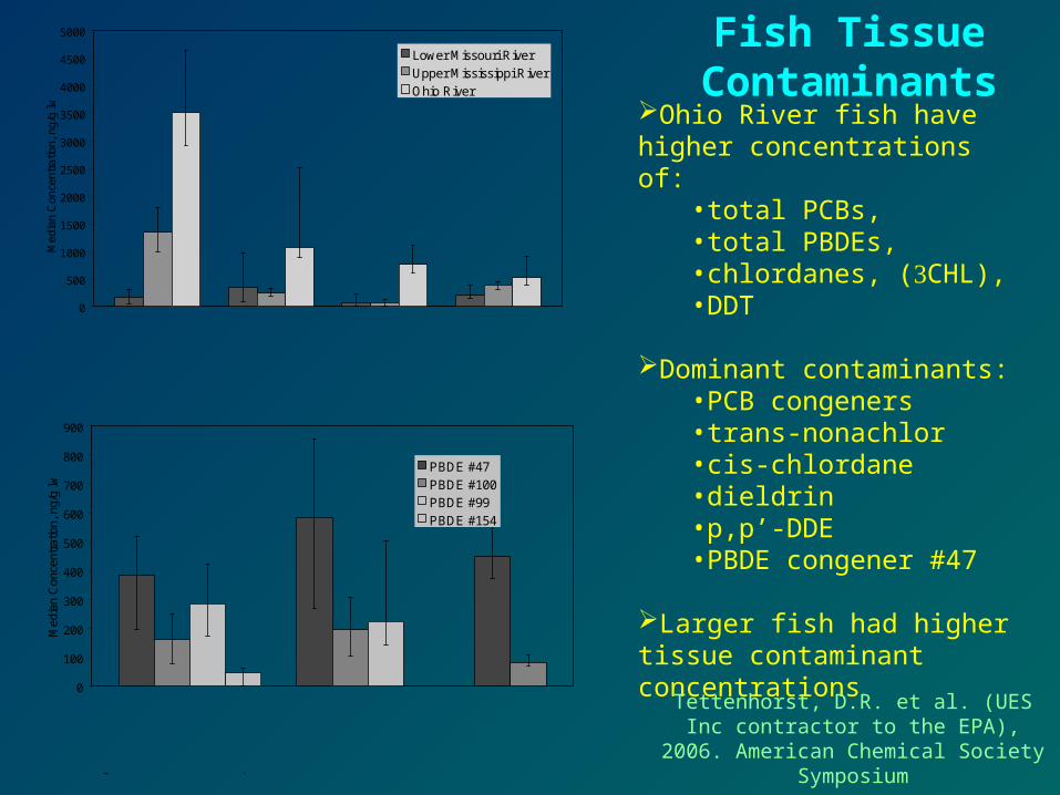
Figure 1. Total PCB congeners (∑PCB), total PBDE congeners (∑PBDE), total chlordanes (∑CHL), and total DDTs (∑DDT) median concentrations for large fish samples from the Ohio, Upper Mississippi and Lower Missouri Rivers.
0
100
200
300
400
500
600
700
800
900
Med
ian
Con
cent
ratio
n, n
g/g
lw
PBDE #47PBDE #100PBDE #99PBDE #154
Large Fish:Freshwater drum
Larger Fish: Sauger
Small Fish:Emerald shiner
Figure 2. Median conger-specific PBDE concentrations and the 95% confidence intervals for two large fish and one small fish species (with n>9) collected from the Ohio River.
Ohio River fish have higher concentrations of:
•total PCBs, •total PBDEs, •chlordanes, (CHL), •DDT
Dominant contaminants:•PCB congeners •trans-nonachlor•cis-chlordane•dieldrin•p,p’-DDE•PBDE congener #47
Larger fish had higher tissue contaminant concentrations
Tettenhorst, D.R. et al. (UES Inc contractor to the EPA), 2006. American
Chemical Society Symposium
Fish Tissue Contaminants
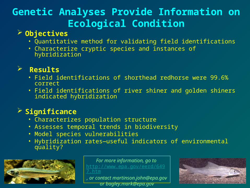
Genetic Analyses Provide Information on Ecological Condition
Objectives• Quantitative method for validating field identifications• Characterize cryptic species and instances of hybridization
Results • Field identifications of shorthead redhorse were 99.6% correct • Field identifications of river shiner and golden shiners indicated
hybridization
Significance • Characterizes population structure • Assesses temporal trends in biodiversity• Model species vulnerabilities• Hybridization rates—useful indicators of environmental quality?
For more information, go to http://www.epa.gov/eerd/6497.htm, or contact [email protected]
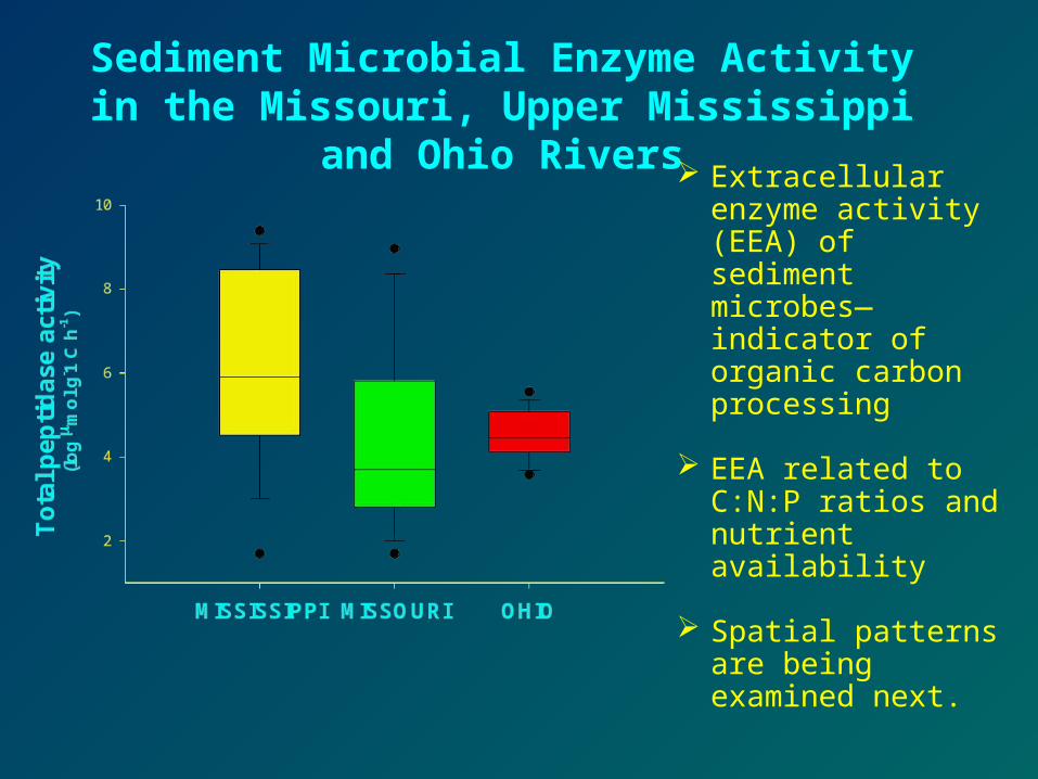
Sediment Microbial Enzyme Activity in the Missouri, Upper Mississippi and Ohio Rivers
Extracellular enzyme activity (EEA) of sediment microbes— indicator of organic carbon processing
EEA related to C:N:P ratios and nutrient availability
Spatial patterns are being examined next.

Chlorophyll a
Mississippi River
Ch
loro
ph
yll
a (
g L
-1)
20
40
60
80
Missouri River
Ch
loro
ph
yll
a (
g L
-1)
20
40
60
80 Ohio River
Ch
loro
ph
yll
a (
g L
-1)
20
40
60
80

Ohio River
0.0
0.2
0.4
0.6
0.8
1.0
1.2
0.00
0.01
0.02
0.03
0.04
0.05
River Mile (from Pittsburg, PA)
0 200 400 600 800 10000
1
2
3
4
5
6
Missouri River
0.0
0.2
0.4
0.6
0.8
1.0
1.2
0.00
0.01
0.02
0.03
0.04
0.05
River Mile (from mouth)
05001000150020000
1
2
3
4
5
6
Mississippi RiverD
iss
olv
ed
N (
mm
ol/L
)
0.0
0.2
0.4
0.6
0.8
1.0
1.2
Dis
so
lve
d P
(m
mo
l/L)
0.00
0.01
0.02
0.03
0.04
0.05
River Mile (from mouth)
02004006008001000
Dis
so
lve
d S
i (m
mo
l/L)
0
1
2
3
4
5
6
Nutrient Chemistry — Downstream Trends

Si:
N
0.1
1
10
100
N:P
Si:
N
0.1
1
10
100
1 10 100
Si:
N
0.1
1
10
100
Si:
P
0.1
1
10
100
1000
10000
Si:
P
1
10
100
1000
10000
N:P
0.1 1 10 100 1000
Si:
P
1
10
100
1000
10000
Stoichiometric Relationships
MississippiRiver
MissouriRiver
OhioRiver

DIN (mmol L-1)
0.01 0.1 1 10
DS
i:D
IN
0.01
0.1
1
10
100
1000
DIP (mmol L-1)
0.0001 0.001 0.01 0.1
DS
i:D
IP
0.1
1
10
100
1000
10000
Mississippi River r2=0.40Missouri River r2=0.65Ohio River r2=0.72
Dissolved Nutrients Control Stoichiometry
Mississippi River r2=0.42Missouri River r2=0.75Ohio River r2=0.56

Comparison with a
Previous Study
MS MO OHThis study DIN 327 136 242
DIP 18 11 6.8DSi 1797 1691 1126N:P 25 24 53Si:N 6.9 32 4.8Si:P 14 80 26
Justic et al. (1995)1981-87 data DIN 114
DIP 7.7DSi 108N:P 15Si:N 0.9Si:P 14
1960-62 data DIN 36DIP 3.9DSi 160N:P 9Si:N 4.3Si:P 40
Year 1960-62 Year 1981-87 Year 2004
DIN
(m
mo
l L
-1)
100
200
300
DIP
(m
mo
l L-1
)
5
10
15
Year 1960-62 Year 1981-87 Year 2004
N:P
5
10
15
20
25
Si:
N
0
3
6
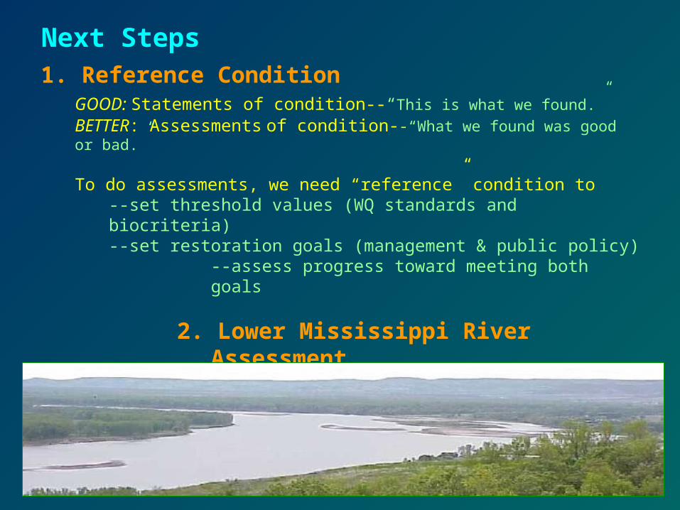
Next Steps1. Reference Condition
GOOD: Statements of condition--“This is what we found.”
BETTER: Assessments of condition--“What we found was good or bad.”
To do assessments, we need “reference” condition to--set threshold values (WQ standards and biocriteria) --set restoration goals (management & public policy)
--assess progress toward meeting both goals
2. Lower Mississippi River Assessment2007 Begin testing EMAP-GRE methods 2008-09 Data collection2010-11 Complete assessment

I. An empirical approach needs data.• Probability design yields full range of conditions—but relatively
few sites have LDC• Targeted designs can increase rate of finding reference sites—
but data can not be used for population estimates• The Target Probability Design (TPD) increases number of least
disturbed sites while optimizing the population assessment
II. Uses abiotic metrics as filters to define which sites have LDC (i.e. reference sites).
III. Verify reference set using biotic indicators
Characterizing and locating least disturbed conditions (LDC)

Gradient
Ab
iotic
ind
ica
tor
Least disturbed / pass / good
Highly disturbed / fail / poor
Fixed criteria
... but, could excludeentire sections of river
A common approach...

Gradient
Indi
cato
r
“Relative to conditions in the area, these are the best.”
A better approach distributes reference conditions along the gradient
“Relative to conditions in the area, these are the worse.”
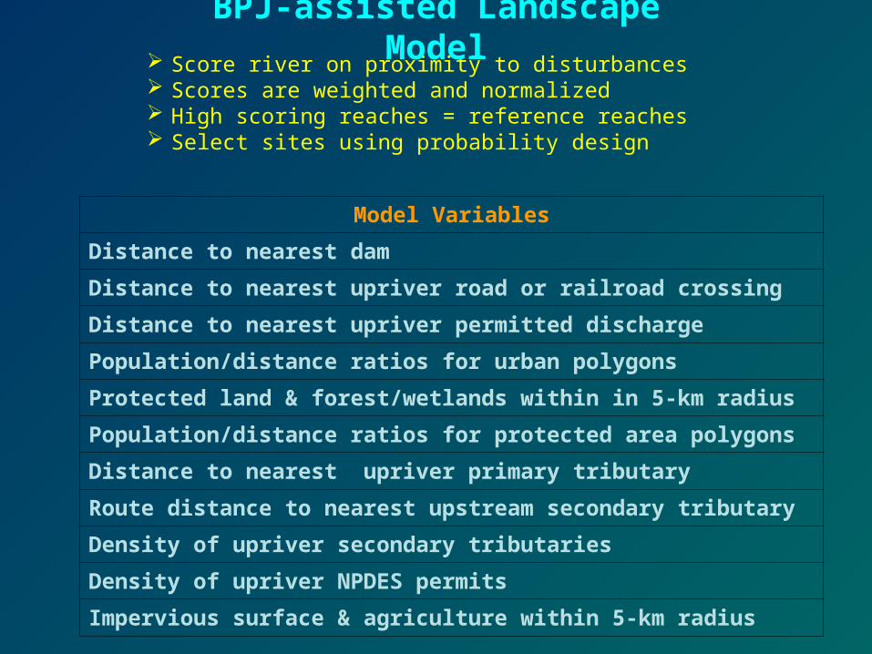
Model Variables
Distance to nearest dam
Distance to nearest upriver road or railroad crossing
Distance to nearest upriver permitted discharge
Population/distance ratios for urban polygons
Protected land & forest/wetlands within in 5-km radius
Population/distance ratios for protected area polygons
Distance to nearest upriver primary tributary
Route distance to nearest upstream secondary tributary
Density of upriver secondary tributaries
Density of upriver NPDES permits
Impervious surface & agriculture within 5-km radius
Score river on proximity to disturbances Scores are weighted and normalized High scoring reaches = reference reaches Select sites using probability design
BPJ-assisted Landscape Model

1 2 3 5 6 7 89
10
4
The further a site is from
disturbances, the higher the
score
Scored as “really good”
Scored as “other”Normalized scores from model

Candidate Reference Reaches
Medium score reach
Low score reach
GIS programmers: Tatiana Nawrocki, Roger Meyer, Matt Starry, and James QuinnComputer Science Corporation

Lower Mississippi River—sample design
TN
MO
MS
AR
LA
LA-LA
MS-LA
MS-AR
TN-MOTN-AR
KYMO-KY
Target 30 sites per State
Statelength (km)
shares with % Sites
Actual sites
LA 808 30
LA 60% 18
MS 40% 12
AR 515 30
MS 65% 20
TN 35% 10
MO 200 30
KY 50% 15
TN 50% 15
KY 15 30
MS 32
TN 5 30
TOTAL 182
•Sites are proportionally distributed within a State
•Sites sampled in interstate sections are used to assess both states

In the end….• Targeted Probability Design makes sense
– Accounts for gradients– Distributes reference sites
• Multi-metric approach– avoids bias of event-drive phenomenon– avoids bias of bad or missing values