Assessing Stakeholder Preferences for Chesapeake Bay Restoration Options: A Stated Preference Discrete

Choice-Based Assessment

Photo: Chesapeake Bay Gateways Network

Rob Hicks1

James E. Kirkley2

Kenneth E. McConnell3

Winifred Ryan2

Tara L. Scott2

Ivar Strand3

1 College of William and Mary, Department of Economics, Williamsburg, VA. 2 College of William and Mary, School of Marine Science, Gloucester Point, VA. 3 University of Maryland, Department of Agricultural and Resource Economics, College Park, Maryland Funding provided by NOAA Chesapeake Bay Office, National Marine Fisheries Service and the Virginia Institute of Marine Science, College of William and Mary.

Assessing Stakeholder Preferences for Chesapeake Bay

Restoration Options: A Stated Preference Discrete Choice-Based Assessment

Funded by: NOAA CHESAPEAKE BAY OFFICE

NATIONAL MARINE FISHERIES SERVICE ANNAPOLIS, MD

AND VIRGINIA INSTITUTE OF MARINE SCIENCE

GLOUCESTER POINT, VA

Completed by: Rob Hicks

James Kirkley Kenneth McConnell

Winifred Ryan Tara Scott Ivar Strand

January 2008

ii

Table of Contents

Section Page List of Tables ..................................................................................................................... iv List of Figures ..................................................................................................................... v Executive Summary ........................................................................................................... vi

1. Introduction..................................................................................................................... 1

1.1 Summary ................................................................................................................... 1 1.2 Some Reasons for Caution........................................................................................ 3 1.3 Status of the Bay ....................................................................................................... 6

2. Goals, Objectives, and Methodology.............................................................................. 8

2.1 Goals and Objectives of Chesapeake 2000............................................................... 8 2.2 Assessing Stakeholder Preferences......................................................................... 10

2.2.1 Estimating preferences for attributes of Bay Restoration ................................ 10 2.2.2 Study Design and Data Collection................................................................... 12

2.2.2.1 Study Attributes: What is being restored versus what people value......... 12 2.2.2.2 Pre-testing and Selection of Attributes ..................................................... 14 2.2.2.3 The Sample: Using stakeholders rather than the general public............... 14

2.3 The Choice Experiment .......................................................................................... 16 2.4 Determining Average Unit Cost of Restoration Attribute ...................................... 18 2.5 Modeling responses to the stated choice questions................................................. 20

2.5.1 The Random Utility Model.............................................................................. 20 2.6 Assessing Budget Allocations................................................................................. 22

3. Preferences and Budget Allocations ............................................................................. 23

3.1 Overview of Results and Empirical Analyses ........................................................ 23 3.2 Survey and Sample Results..................................................................................... 23 3.3 Assessing Preferences and Marginal Values .......................................................... 25 3.4 Multiple Changes in Attributes and Optimal Restoration Bundles ........................ 27

3.4.1 Case 1: No Joint Production and all goods valued directly ............................. 28 3.4.2 Case 2: Joint Production .................................................................................. 28

3.5 Budget Allocations, Competing Restoration Options, and Maximizing Utility..... 29 3.6 Applicability or Estimated Budget Allocations ...................................................... 34

4. Summary and Conclusions ........................................................................................... 35

References......................................................................................................................... 39 Appendix........................................................................................................................... 40

iii

List of Tables Table Page

Table 2.1. Major Goals and Sub goals, Estimated Restoration Costs, and Projected Funding (Millions of 2007 Dollars)............................................................................ 9

Table 2.2. Restoration Goals and Current Status for C2K............................................... 14 Table 2.3. Sampling Frames and Actual Sample for Stated Preference Survey.............. 16 Table 2.4. Per Unit Bay Restoration Costs ...................................................................... 19 Table 3.1. Percent of Respondents Indicating Level of Importance of Regional Issue... 23 Table 3.2. Respondents’ Familiarity with the Bay (Percent)........................................... 24 Table 3.3. Percent of Respondents Indicating Usage Level of Bay................................. 24 Table 3.4. Percent of Respondents Expressing Level of Concern about Bay Resources 25Table 3.5. Parameter Estimates for Three Specifications of the Utility Modela,b............ 26 Table 3.6. Levels of Utility and Restoration Given Different Constraints ...................... 33 Table 3.7. Allocations (Million $) For Restoration Options Given Different Constraints

................................................................................................................................... 34

iv

List of Figures Figure Page

Figure 1.1. Restoration Activities and Ecosystem Outputs ............................................... 5 Figure 2.1. A Stated Preference Question........................................................................ 18

v

Executive Summary Chesapeake 2000 or C2K is a multi-jurisdictional agreement between the states of Virginia, Maryland, Pennsylvania, the District of Columbia, the Chesapeake Bay Commission and the U.S. Environmental Protection Agency, representing the federal government, to restore the health of the Chesapeake Bay’s ecosystem. This agreement commits the participants to achieve five major restoration goals, 22 sub-objectives or categories, and 102 specific commitments or restoration activities. The five major goals are the following: (1) restore and protect natural living resources; (2) restore and protect vital habitat; (3) restore and protect water quality; (4) promote sound land use; and (5) promote stewardship and community engagement. The sub-categories and specific commitments impose specific restoration requirements relative to each of the five major categories. In 2003, the Chesapeake Bay Commission, utilizing a panel of experts, estimated the cost of achieving all five major objectives equaled approximately $18.7 billion, which equals approximately $21.0 billion in 2007 dollars. Unfortunately, all partners of C2K only committed $5.9 billion ($6.6 billion in 2007 dollars) in funding to achieving the five major objectives. There is, thus, a deficit of $12.8 billion or $14.4 billion in 2007 dollars. The funding available to achieve the goals of C2K is of considerable concern because the single sub-objective of the category of reducing nutrients and sediments requires more than $12.0 billion in 2007 dollars, and this is a major requirement for restoring the health of the Bay’s ecosystem. The cost of restoring the Bay complicates the choices and levels of restoration options. Given the large deficit for achieving the goals and objectives of C2K, it is necessary to assess how restoration might proceed. The available level of funding is simply inadequate for achieving all the goals and objectives necessary to restore the Bay’s ecosystem. In this study, we attempt to provide an assessment of how available funds might be distributed among the restoration goals and objectives in a manner, which generates the greatest social value. Restoring the ecosystem of the Bay is as much a social and economic issues as it is a scientific issue. That is, what restoration options do stakeholders desire given a limited budget and the cost of restoration? In this report, we present an approach for comparing Chesapeake Bay options based on stakeholder preferences and restoration costs, and a subsequent assessment of social welfare corresponding to different levels and mixes of restoration options. Our social welfare metrics, however, are not absolute or cardinal measures; there are instead ordinal or qualitative metrics (e.g., a welfare value of 200 relative to 100 implies that 200 is higher, but not necessarily that social welfare equals 200 and is twice as high as welfare equaling 100). We demonstrate how this empirical framework might be used to help policy-makers determine the best restoration options and allocations of available funds. We utilize a method known as the stated preference method in which survey respondents reveal preferences for Bay restoration options and their potential levels.

vi

Unfortunately, because of the large number of restoration goals, objectives, and specific commitments and the fact that many options have no stated or desired target levels, we cannot deal with all the options. We instead focus on the major restoration options necessary to restore the Bay, and those with outputs easily understandable by stakeholders. Our selected restoration options include oysters, blue crabs, shad, wetlands, nutrient and sediment levels, and chemical contaminant levels. The latter two, however, are expressed in terms of understandable outputs—seafood advisories for chemical contaminant reductions and beach advisories for nutrient and sediment reductions. Our survey questionnaire also informs the respondent about the linkages between seafood advisories and chemical contaminant levels and beach closures and nutrient and sediment levels. Outputs for the other options are stated in terms of biomass or number of fish and acres of wetlands. Because of the large number of potential stakeholders and high cost of conducting a large-scale survey, we primarily surveyed well-informed stakeholders that likely represent a much larger constituency (e.g., the desired options and level of a local or state planner likely reflects the desired options and restoration levels for his or her community). We confineed our survey to stakeholders in Maryland and Virginia, and include 15 broad stakeholder groups: (1) women’s clubs, (2) native Americans, (3) non-governmental organizations (NGOs and ENGOs), (4) recreational fishing organizations, (5) cruise operators, (6) marine transport companies, (7) federal officials, (8) local government staff, (9) local board members, (10), local elected officials, (11) state agency officials, (12) fish processors and producers, (13) watermen, (14) charter and party boat operators, and (15) marine and related scientists and economists and social scientists. Prior to asking questions about the preferred restoration options and levels, we asked four broad questions to determine the familiarity of respondents with the Bay problems, and to assess stakeholder concerns about other problems in the region. The first question requested respondents to indicate their level of concern about other problems in the region (e.g., the importance of reducing crime in the region; improving education in primary and secondary schools; decreasing air pollution; finding ways to reduce state taxes; and restoring the environmental quality of the Bay). Of the five issues, restoring the quality of Bay was viewed as extremely important by a large majority of the respondents. The least important issue was finding ways to reduce state taxes. Individuals were also asked to state their familiarity with the Bay and its problems; 66.1 % of the respondents indicated they were very familiar with the Bay. The third question attempted to obtain information on usage levels of the Bay by respondents. Oddly, a large number of respondents reported relatively moderate to low usage levels of the Bay. The fourth question asked respondents about their level of concern about the Bay’s resources; 52.4 % of the respondents indicated they were extremely concerned; 36.5 % of the respondents indicated they were very concerned; and 11.2% indicated they were either somewhat concerned or not concerned at all.

The next question in the survey requested respondents to indicate their restoration options and desired levels. Utilizing data obtained from this question, we estimated random utility models (RUM), which facilitated the determination of preferences for

vii

bundles of restoration options with different levels of attributes for each bundle (e.g., restore the oyster population by 50 %; maintain the current level of blue crabs; and fully restore the shad population). This same question was asked three times in the questionnaire with each question having different levels of the attributes of each restoration option. Also, there were 15 versions of the survey, with each version containing different levels of the attributes; each stakeholder group, but not individual stakeholder, received up to 15 different versions of the survey. The random utility models provided estimates of probabilities for each bundle, which can be translated into level of preferences or social welfare. Again, it must be stressed, however, that these metrics are ordinal and not cardinal. Our RUM models are actually models expressing utility or social welfare as a function of the different bundles of restoration options. We also estimated the feasible restoration options and levels, which maximize social welfare subject to an overall restoration budget constraint. The overall budget constraint was set equal to the funding available for the six options, which equaled $2.6 billion in 2007 dollars. This allowed us to determine the level of funding to allocate to each of the restoration options such that social welfare or satisfaction to society was maximized. In this case, we maximize utility subject to a budget constraint, given per unit restoration costs. We solved four basic optimization problems: (1) maximize utility subject to budget and non-negativity constraints; (2) maximize utility subject to a budget constraint and constraints requiring certain levels of nutrient reduction and chemical contaminant reduction; (3) maximize utility allowing for a $1.0 billion increase and decrease in available funding; and (4) maximize utility subject to the budget constraint and additional constraints prohibiting more funds than recommend by the Chesapeake Bay Commission for each restoration option (e.g., the Bay Commission recommended that $101.5 million was required to restore the oyster population to ten times its level in 1994; this problem constrained any funding for oyster restoration higher than $101.5 million). The first problem, the least restrictive problem, which maximizes social welfare regardless of desired target levels, indicated that stakeholders preferred higher levels of restoration than suggested by the Bay Commission for oysters, blue crabs, and shad. Stakeholders desired lower than stated target levels for wetlands, nutrient reduction, and chemical contaminant reduction. The solution to the problem with constraints on the restoration goals (i.e., cannot generate a solution requiring a higher level than listed as the target goal) yielded an allocation of funds such that all target levels, except those for nutrient and chemical contaminant reductions, were achieved. The lowest level of social welfare corresponded to the problem having constraints requiring expenditures on each restoration option to be less than or equal to that recommended by the Bay Commission. Although the results are very illuminating and quite interesting, it must be understood that there are some serious limitations of the analyses. First, it is highly likely that many respondents either did not adequately understand the questions related to nutrient and chemical contaminant reduction or are not familiar with the importance of reducing nutrients, sediments, and chemical contaminants. Second, there is a problem of jointly produced goods or the fact that some restoration outputs are inputs into other

viii

restoration options. For example, reducing nutrients and sediments helps restore oysters, blue crabs, shad, and wetlands, while also serving as inputs to these other restoration options. It is extremely difficult to adequately assess social welfare in the case of jointly produced ecosystem goods and services. Another problem is how representative was our survey of the general population of stakeholders in the region; we have no information to adequately assess this concern. An additional major limitation relates to restoration costs. On one hand, the most important restoration options are very costly, and stakeholders, particularly if they are unfamiliar with the importance of restoration options like nutrient reductions, may have simply viewed this option as too expensive. Then, there is the issue of calculating per unit cost of restoration options and levels. We used the cost projections provided by the Bay Commission divided by the desired restoration target levels, but in some cases, our target levels had to be converted to outputs most understandable by the general public (e.g., beach closures for nutrient reductions); in this case, the per unit restoration costs may have been viewed as extremely expensive by some stakeholders. Another problem related to cost involved the jointly produced nature of a given restoration option, and our inability to correctly derive a cost for jointly produced goods (e.g., the joint per unit cost of nutrient reductions and oyster restoration). Despite these limitations, the framework developed for this study indicates a strong need for an integrated model, where models of the Bay ecosystem and human preferences can be integrated to yield more definitive policy guidance. In addition, the empirical results provide benchmarks for examining alternative restoration targets, options, and funding. An additional important result is that the study indicates that stakeholders and the general public need to be better informed about the need for reducing nutrients, sediments, and chemical contaminants. Stakeholders appeared to adequately understand restoration options for living natural resources, but not for reducing nutrients, sediments, and chemical contaminants.

ix

1. Introduction 1.1 Summary A multi-jurisdictional effort to restore the ecosystem of the Bay has been conducted for more than 20 years. The Chesapeake Bay Agreement was signed into effect in 1983. Signatories represent the state of Maryland; the Commonwealths of Pennsylvania and Virginia; the District of Columbia; the U.S. Environmental Protection Agency representing the U.S. government; and the Chesapeake Bay Commission representing Bay state legislators. The Plan is committed to reducing pollution, restoring habitat, and managing fisheries. Over the past 20 years, the goals and objectives have evolved, reflecting new information, scientific findings and progress or the lack thereof in improving the Bay. There have been numerous subsequent agreements with Chesapeake 2000 being the most current.

The overall cost of restoration complicates choices of restoration options. In

2003, the Chesapeake Bay Commission produced the report “The Cost of a Clean Bay: Assessing Funding Needs Throughout the Watershed.” The total estimated cost was $18.7 billion, while the funding available equaled only $5.9 billion- a budget shortfall of $12.8 billion even after adjusting for all local, state, regional, federal, and private sources of funding. Any current restoration plan cannot achieve all goals. Given the shortfall in funding, there are two paramount policy questions for Bay restoration. The first question, and the one we address in this report, asks how restoration might proceed, given insufficient resources for achieving all goals. This question involves how difficult (and costly) it is to reach the individual goals, and which goals have the greatest social value. It is as much a social and economic issue as it is a scientific issue. In simple terms, what restoration activities do stakeholders desire, given the limited budget? While this will be a political decision, it will be informed by the preference of citizens and stakeholders. In this report we provide some evidence on these preferences that can be useful in forming a political solution. The second question, also important yet not dealt with in this report, concerns the formulation of policy that reduces the costs of achieving the Bay goals. Environmental policy that reduces pollution in least-cost ways can be viewed as freeing resources for more expansive restoration efforts or other uses of the savings.

In this report, we present an approach for comparing Chesapeake Bay restoration options based on stakeholder preferences for the Bay’s resources. We show how this empirical approach might be used to help policy-makers decide what restoration option is best and where the next restoration dollar spent yields the greatest public benefit. Throughout this report we highlight the important linkage and the analytical complications stemming from the interplay between restoration activities, a natural system that translates these restoration activities into ecological outcomes, and ultimately the public benefits from Bay restoration.

1

We probe individual preferences by having survey respondents choose among alternative scenarios for improving Bay quality. These choices reveal preferences. This approach, known as the stated preference method, uses discrete choice statistical tools outlined in Louviere et al. (2000. The estimated preferences describe how respondents would make trade-offs among the Bay goals. With these preferences and with independent information on the costs of achieving various goals, we compute the budget allocations among goals that would represent the best use of budget for the stakeholders. We find that stakeholders prefer the well-known resource stocks in the Bay (e.g. oysters, crabs, and fish stocks) compared to other indicators of system-wide habitat or water quality improvement (e.g. consumption advisories, beach closures, and wetland restoration). This result demonstrates that many of the most expensive restoration activities related to nutrient runoff reductions, habitat set-asides, and riparian buffers are not as highly valued as well-known Bay resources. Further, it bears mentioning that since this report focuses on stakeholders- presumably having better knowledge about the full array of restoration outcomes than the public- our results demonstrate that large-scale water and habitat programs are surely the toughest sell.

The analytical approach in this report follows from the environmental valuation literature, where the value of some environmental attribute is based on what individuals are willing to give up to have a restored bay. If individuals are not willing to give up anything to restore an organism in the Bay and the presence or absence of the organism has no affect on other members of the Bay ecosystem, then a restoration program aimed at this organism has no public benefits. If, however, the organism is a key member of the food web upon which crabs and other organisms depend, then the public may benefit from restoring this organism since its restoration will have positive affects on organisms and systems the public does value (e.g. crabs, oysters, etc.). Consequently, a key component of valuing an ecosystem restoration program is the science of how parts are related and how restoring parts of the ecosystem leads to ecological outcomes that people care about. Currently, significant uncertainty exists concerning predicting outcomes based on restoration activities making a complete accounting for economic benefits from restoration difficult.

Related to this issue is valuing the benefits from restoration programs when a program may consist of 102 commitments; there are simply too many ecosystem attributes for individuals to consider at one time. Even 22 sub goals are typically beyond comprehension of most individuals. Many of the restoration objectives or commitments are expressed in highly scientific terms, making it difficult for many stakeholders to adequately understand the objectives, and thereby making a study of stakeholder preferences for these objectives exceedingly difficult. A good example is the objective of reducing nutrients and sediments. Scientists and individuals who deal frequently with nutrient reduction issues may be able to express preferences for nutrient reductions because they understand the interactions between water quality conditions in the Bay and how nutrient levels impact well known resources (e.g. oysters) and the current levels of nutrients. Other stakeholders, however, may have little or no understanding of the importance of nutrient reduction and fail to appreciate how programs aimed at reducing nutrients impact other ecosystem components.

2

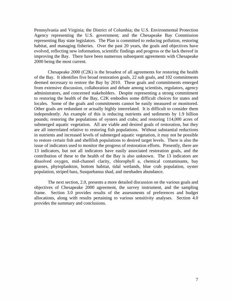
Other research on measuring ecosystem benefits has often tackled ecosystems having fewer components and has been able to educate the public about the workings of interrelated parts of the ecosystem prior to measuring preferences. Given the many components of a potential Bay restoration program (we term these “inputs”) and the many organisms and systems that may be affected, this approach is simply not feasible. The approach we take focuses on key ecosystem “outputs” that might be considered bell-weather indicators of outcomes related to a restoration program. Figure 1 depicts the relationship between “inputs” and “outputs”. The restoration activities (“inputs”) are conducted and the natural system translates these efforts into environmental outcomes that society values. It is possible that some “inputs” are valued directly by society (e.g. an acre of wetland restoration) whereas others may only serve to produce “outputs” that society does value.

Thinking of measuring preferences for Bay restoration in this way helps to reduce

the dimensions of the problem. By construction, the “outputs” we focus on in our empirical work are 1) well-known to stakeholders in the Bay, and 2) are considered by scientists to be important indicators of overall ecosystem health. Consequently our work should be viewed as measuring stakeholder preferences for restoration outcomes that could result from numerous restoration policies directed at each of the Bay’s hundred or so systems.

1.2 Some Reasons for Caution

Valuing ecosystem services for the Bay is a useful but hugely complex undertaking. Our approach might best be viewed as exploratory. We have touched on a couple of caveats above. The basic problems stem from the following issues:

1. Uncertainty in restoration success and time until recover; 2. Restoration costs and joint production and valuation of inputs and outputs; and 3. Sampling of stakeholders versus the general public. Attempting to determine the value of the services of the Bay ecosystem can be

compared with measuring the value of an imaginary large but cranky factory. Suppose the factory produces goods well known to consumers—TV’s, ipods, calculators, etc. Consumers are quite able to determine the value of these finals goods. But if the goods are available at uncertain future dates—next month, next year, a few years, a decade, then the valuation becomes quite difficult. The same holds for Bay ecosystem services, which will arrive at uncertain future dates even when restoration works. And if we look inside the factory at some of the factors of production, say an assembly line or the electricity used in production, we can be quite sure that consumers will have no inkling of how to value the inputs. Valuing Bay ecosystem services presents the same problems. Many of the goals of the Bay restoration are not final services, but inputs that help produce these services. For example, citizens may not understand the role of subaquatic vegetation in sustaining the blue crab population even though they have a well-formed sense of what the crabs themselves are worth. There is an additional problem with mixing inputs and outputs in valuation of Bay restoration goals—double counting of returns. Most inputs—

3

subaquatic vegetation and reduction in nitrogen loadings—produce several services. The sum of the values of inputs and outputs will exceed the value of the final services.

This feature of the Bay restoration—the various inputs and outputs—makes good

sense for sound ecological policy, but requires some adapting of the standard approach to valuation of environmental services. To understand the complex questions implicit in Bay restoration, we have designed a sample frame of respondents who are well informed about the Bay. We call these respondents stakeholders. We expect the stakeholders’ frame, which includes scientists, watermen and policy makers, to understand the role of nitrogen, subaquatic vegetation, and other inputs about which the public would be poorly informed. This formation of the sample frame has a drawback, however. The sample frame is not representative of the general public and may have quite different values for the final services of the Bay. Nevertheless, we pursue our valuation exercise as a means of gaining some understanding about how to use the available funds for Bay restoration. But we consider the document a report on some useful ways of tactics for pursuing Bay restoration, not a set of precise values of ecoservices for the Bay.

The problem of inputs and outputs is complicated by costs. Many of the high

costs of inputs include the costs of outputs. Determining an optimum mix of restoration activities requires information on the total and per unit cost of restoration. Many of the restoration options are extremely costly; for example, the cost of nutrient and sediment reduction is estimated to be $10.8 billion. The proposed objective is to reduce nutrients and sediments by approximately 1.9 billion pounds. This equates to an average per unit cost of $5.70 per pound. Yet a reduction in nutrients provides a joint benefit in that it potentially benefits many “outputs”- submerged aquatic vegetation, water-based recreation, and marine resources. For other restoration options, the total cost is known but the per unit cost cannot be directly calculated or must be developed in a proxy format. For example, the per unit cost of reducing chemical contaminants is not known since there are likely a myriad of activities that can be used to achieve a goal. Given incomplete and at times nonexistent information on costs, our policy guidance on what restoration outcomes are best could undoubtedly be improved with better cost information.

4

Figure 1.1. Restoration Activities and Ecosystem Outputs

An important limitation of our analysis relates to the uncertainty associated with

ecosystem restoration. Restoration activities may not be successful at all or may have unanticipated side effects. Some activities may lead to much faster recovery of some resources while others may take decades. Incorporating uncertainty into an empirical study of stakeholder preferences, while important, complicates the task even more. Our analysis ignores the uncertainty of restoration by asking respondents to consider certain outcomes.

Our study relies heavily on a sample of individuals who are knowledgeable about the Bay because they have worked as scientists on Bay issues or have been involved in the political process of improving the Bay or used the Bay to earn a living. We have called this group ‘stakeholders’, though this is a partially inaccurate characterization of our sample. The true stakeholders are all tax payers who provide the funds for Bay restoration and the households who use the Bay and its products. Because of funding limitations, we are unable to include all stakeholders. We do, however, include many other stakeholders, such as charter boat operators, various government officials and employees, recreational anglers, American Indians, various environmental organizations, and other interested stakeholders.

An advantage of focusing on these stakeholders, who might more aptly be called

vested interests, is that their vocations or avocations depend on or focus on the functioning of the Bay. Consequently, these stakeholders probably possess more information and have a better understanding of the inter-related nature of the Bays natural systems. For example, Bay restoration goals include targets such as the female biomass of crabs or acres of sub-aquatic vegetation. These Bay restoration goals reflect a well-functioning ecosystem. This type of information known by stakeholders, makes the task of measuring preferences for an ecosystem as complicated as the Bay much easier. In essence, to extrapolate our results to the public at-large, one must assume that preferences of well-informed stakeholders provide useful information of the value of the Bay ecosystem to the universe of stakeholders—taxpayers and citizens currently as well as

5

those of future generations. For example, the general public values the ability to harvest and consume blue crabs, but may not know how sub-aquatic vegetation enhances the crab population. The sampled knowledgeable stakeholder can be expected to be knowledgeable about the relative value of ecosystem functioning as well as the final services of the Bay. Consequently our results, while likely indicative of how restoration might benefit the public at-large, are hardly definitive. Care should be exercised when using this report for restoration policy making.

Even with the aforementioned caveats, the approach we outline here does point

towards an integrated model where models of the Bay ecosystem and human preferences can be integrated to yield more definitive policy guidance for Bay restoration programs. 1.3 Status of the Bay

The Chesapeake Bay is the largest estuary in North America. The accompanying watershed runs through six states, including New York, Pennsylvania, Delaware, Maryland, Virginia, and West Virginia, and the District of Columbia.1 More than 64,000 square miles of land drain into the watershed, which has a population of about 16 million people. The watershed encompasses approximately 66,000 square miles of land. Formally, the Bay is about 200 miles long and runs from Havre de Grace, MD to Norfolk, VA. The Bay supports more than 3,600 species of plants, fish and animals, including 348 species of finfish, 173 species of shellfish, and over 2,700 plant species. The Bay provides a wide range of recreational opportunities for the millions of households living in the Bay basin and supports numerous commercial activities such as fishing and shipping. Over the last fifty years, the health of the Bay has declined. Concern over the deteriorating functioning of the Bay has lead to a series of efforts to improve the quality of the Bay. The Bay’s health is assessed based on four broad aggregate indicators for capturing the status of animals, habitat, plankton and bottom dwellers and water quality. A multi-agency effort including various state and federal agencies and universities, formed to assess the habitat health of the Bay, gave the health of the Bay a grade of D+ for 2006.2 Notable concerns focused on declines in habitat, water quality, fish and shellfish populations, and contaminants. A multi-jurisdictional effort to restore the ecosystem of the Bay has been conducted for more than 20 years. The Chesapeake Bay Agreement was signed into effect in 1983. Signatories represent the state of Maryland; the Commonwealths of 1 Data and descriptive statistics relating to the Chesapeake Bay and Watershed are from the Chesapeake Bay Program, http://www.chesapeakebay.net/wshed.htm 2 The various agencies or organizations contributing to the development of the report card are the following: Chesapeake Bay Program, University of Maryland Center for Environmental Science, National Oceanic and Atmospheric Administration, Maryland Department of Natural Resources, Virginia Department of Environmental Quality, Virginia Institute of Marine Science, Versar Incorporated, US Environmental Protection Agency, Maryland Department of the Environment, Interstate Commission on the Potomac River Basin, Old Dominion University, and Morgan State University.

6

Pennsylvania and Virginia; the District of Columbia; the U.S. Environmental Protection Agency representing the U.S. government; and the Chesapeake Bay Commission representing Bay state legislators. The Plan is committed to reducing pollution, restoring habitat, and managing fisheries. Over the past 20 years, the goals and objectives have evolved, reflecting new information, scientific findings and progress or the lack thereof in improving the Bay. There have been numerous subsequent agreements with Chesapeake 2000 being the most current. Chesapeake 2000 (C2K) is the broadest of all agreements for restoring the health of the Bay. It identifies five broad restoration goals, 22 sub goals, and 102 commitments deemed necessary to restore the Bay by 2010. These goals and commitments emerged from extensive discussion, collaboration and debate among scientists, regulators, agency administrators, and concerned stakeholders. Despite representing a strong commitment to restoring the health of the Bay, C2K embodies some difficult choices for states and locales. Some of the goals and commitments cannot be easily measured or monitored. Other goals are redundant or actually highly interrelated. It is difficult to consider them independently. An example of this is reducing nutrients and sediments by 1.9 billion pounds; restoring the populations of oysters and crabs; and restoring 114,000 acres of submerged aquatic vegetation. All are viable and desired goals of restoration, but they are all interrelated relative to restoring fish populations. Without substantial reductions in nutrients and increased levels of submerged aquatic vegetation, it may not be possible to restore certain fish and shellfish populations to desired target levels. There is also the issue of indicators used to monitor the progress of restoration efforts. Presently, there are 13 indicators, but not all indicators have easily associated restoration goals, and the contribution of these to the health of the Bay is also unknown. The 13 indicators are dissolved oxygen, mid-channel clarity, chlorophyll a, chemical contaminants, bay grasses, phytoplankton, bottom habitat, tidal wetlands, blue crab population, oyster population, striped bass, Susquehanna shad, and menhaden abundance. The next section, 2.0, presents a more detailed discussion on the various goals and objectives of Chesapeake 2000 agreement, the survey instrument, and the sampling frame. Section 3.0 provides results of the assessments of preferences and budget allocations, along with results pertaining to various sensitivity analyses. Section 4.0 provides the summary and conclusions.

7

2. Goals, Objectives, and Methodology 2.1 Goals and Objectives of Chesapeake 2000

In 1983, the states of Virginia, Maryland, Pennsylvania, the District of Columbia, the Chesapeake Bay Commission, and the U.S. Environmental Protection Agency (representing the Federal Government), agreed to protect and restore the Chesapeake Bay ecosystem by establishing the Chesapeake Bay Program. The Bay Program was endorsed again in 1987. For over 20 years, the signatories to the agreements have sought to restore the health of the Bay.

The Bay program has led to considerable effort towards restoring the Bay and

some significant improvements. But the pressure on the Bay from population increases and economic growth is relentless. Considerably more effort is necessary to address the many complex issues related to the ecosystem. In 2000, the signatories of the original Bay Program reaffirmed their commitment to restoring the Bay. Chesapeake 2000 (C2K) is the most comprehensive, to date, initiative to restore the health of the ecosystem. Chesapeake 2000 has five major goals or objectives; 22 sub goals or subcategories; and 102 specific commitments (Table 2.1). The period of restoration activity is 2003 through 2010.

This comprehensive restoration effort, however, comes with a substantial price

tag. In a report by the Chesapeake Bay Commission (2003), a panel of experts estimated the cost of restoring the Bay to be $18.7 billion, which equals approximately $21.0 billion in 2007 when adjusted for inflation (all figures in 2007 dollars).3 Unfortunately, revenue projections indicate that only $6.6 billion in 2007 dollars will be available between 2003 and 2010. There is a deficit or unfunded gap of $12.8 billion.4

Of the 22 sub goals, the most expensive is nutrient and sediment reduction, which

has a projected cost of $10.8 billion (Table 2.1). The second and third most expensive sub goals are improving transportation ($1.3 billion), and increasing fish passages to enhance the populations of migratory and resident fish ($1.2 billion). There are projected deficits for all sub goals except transportation, air pollution, and partnerships. That is, the projected revenues are less than the estimated restoration costs. There is, of course, no need to provide funding for each goal separately. As we will see in Chapter 3, considering the goals and their costs jointly will provide the most effective use of financial resources for restoring the Bay.

Despite the enormous costs of restoring the Bay’s health and insufficient funding, there are several other aspects of C2K, which limit achieving the stated goals and sub goals. One major problem is that many of the goals, sub goals, and 102 specific 3 These cost figures are essential the costs of command and control approaches to reducing pollution. A critical issue, one that we do not address, concerns the many and various ways of using incentives to reduce costs. 4 The $12.8 billion gap pertains to 2003 levels. All additional summaries and analyses in this report are in terms of 2003 costs and revenues.

8

commitments lack quantifiable or well-defined targets. For example, the sub goal of reducing exotic species is to (C2K, page 2) “Work cooperatively with the U.S. Coast Guard, the ports, the shipping industry, environmental interests and others at the national level to help establish and implement a national program to substantially reduce and, where possible, eliminate the introduction of non-native species carried in ballast water.” Table 2.1. Major Goals and Sub goals, Estimated Restoration Costs, and Projected Funding (Millions of 2007 Dollars)

Goal/Sub-Goal Projected Costs

Projected Funding

Deficit

Living Resource Protection and Restoration Oysters 125.33 101.52 23.81 Exotic Species 23.58 12.47 11.12 Fish Passage 1,398.70 58.40 1,340.30 Multi-species Management 13.36 7.52 5.84 Crabs 22.01 11.57 10.44

Total 1,582.98 191.47 1,391.51 Vital Habitat Protection and Restoration -

Submerged Aquatic Vegetation 44.70 7.41 37.28 Watershed 711.42 249.42 462.00 Wetlands 275.92 129.37 146.55 Forests 122.52 108.59 13.93

Total 1,154.56 494.79 659.76 Water Quality Protection and Restoration - - -

Nutrients and Sediments 12,136.82 2,132.58 10,004.25 Chemical Contaminants 578.57 167.33 411.24 Priority Urban Waters 50.31 19.20 31.11 Air Pollution 92.98 92.98 - Boat Discharge 9.10 8.09 1.01

Total 12,867.78 2,420.18 10,447.61 Sound Land Use - - -

Land Conservation 1,991.08 1,204.64 786.44 Development, Redevelopment, 1,094.81 664.59 430.22 Transportation 1,465.63 1,465.63 - Public Access 120.50 86.02 34.48

Total 4,672.02 3,420.88 1,251.13 Stewardship and Community Engagement - - -

Education and Outreach 166.43 25.04 141.39 Community Engagement 125.89 29.98 95.90 Government by Example 450.66 14.15 436.51 Partnerships 0.11 0.11 -

Total 743.09 69.29 673.80 Total of All 21,020.43 6,596.61 14,423.81

9

The sub goal for crabs is to “Establish harvest targets for the blue crab fishery and begin implementing complementary state fisheries management Baywide.” Similarly, the sub goal of reducing chemical contaminants is not well quantified. The sub goal is in terms of partial or river-wide impairments, where impairments are characterized by bio-accumulative contaminants in fish tissue for Maryland and Virginia.

Assessment of the Bay targets is further complicated by the interrelatedness of the goals and sub goals. Some goals may not be realized unless other objectives or goals are satisfied. For example, it is unlikely that full restoration of oysters and crabs is possible without reductions in both nutrient and chemical contaminant levels. Once these reduction goals are satisfied, however, other restoration activities are necessary to restore the populations of oysters and crabs. Little is to be gained from restoring wetlands if nutrient, sediment, and contaminant levels are not reduced. Restoring wetlands, however, can help reduce the levels of nutrients and sediments in the Bay. We must, then, view many of the sub goals as interrelated activities. That is, realizing one sub goal may help to realize several other sub goals. Alternatively, realizing some of the sub goals produces intermediate outputs, which become inputs necessary for realizing other goals and sub goals.

The targets of C2K were constructed with the laudable goal of restoring the Bay

but without a clear sense of costs or available funding.. The projected funding is only $6.6 billion, less than a third necessary for full ecosystem restoration. Given this shortcoming in financing, policy makers will need to choose the goals worth pursuing. In the next section, we review a method of determining budget allocations among sub goals such that stakeholders are as satisfied as possible, given available funding. The approach facilitates an assessment of stakeholder satisfaction given different desired levels of sub goals, different levels of available funding, and recommended budget allocations to some of the sub goals when funding levels to other sub goals is required by regional authorities. 2.2 Assessing Stakeholder Preferences Determining preferences for goods and services, particularly goods and services of an ecosystem, can be accomplished using numerous methods.5 In this study, however, we use a stated choice method, which enables us to determine preferences for a bundle of attributes resulting from Bay restoration activities. We caution that regardless of the apparent rigor of the quantitative methods analysis and the subsequent numerical assessments, the results are best interpreted as indicative rather than definitive of the kinds of preferences stakeholders have. As we point out in the introduction, the complex interrelatedness of the attributes and the costs limits our confidence in the specific results. 2.2.1 Estimating preferences for attributes of Bay Restoration

The stated preference approach for obtaining empirical profiles of individual preferences relies on sampled individuals’ responses to hypothetical scenarios involving 5 Mithcell and Carson (1989), Louviere et al. (2000), and Bockstael and McConnell (2007) provide a comprehensive discussion on methods for assessing preferences, as well as extensive references.

10

different levels of environmental amenities. The hypothetical scenarios are described in survey instruments. The instruments describe Bay restoration scenarios with a variety of different attributes, and then ask the respondent to choose the best of alternatives. Stated preference techniques have two major classes of elicitation techniques that would let us estimate preferences for restoration. The first type, contingent valuation, measures the value of a change from the status quo to some other state of the world (Mitchell and Carson, 1989). One example would be the case of a researcher asking anglers to consider their current trip, and then ask them their willingness to pay to avoid a reduction in the creel limit of a desirable species. For our problem, the technique is not well suited to measuring preferences for all of the attributes of Bay restoration because the approach can typically model only one or two attributes.

We adopt the choice experiment approach of stated preferences. In this method,

respondents choose among alternatives that are described by their attributes, where in our case the attributes are goals of the Bay restoration plan. This approach, which has been used for several decades in marketing private goods, has been applied for some time to environmental problems. First attributed to Louviere et al. (2000), this approach has been applied to a wide array of environmental management problems. Like contingent valuation, the choice experiment approach can be applied to Bay restoration to obtain information about preferences by analyzing responses to hypothetical restoration scenarios. This approach considers Bay restoration as equivalent to improving a bundle of attributes that describe the ecosystem functioning. This idea is familiar to anyone who purchases market goods which are defined by their attributes. For example a car can be described in terms of make, color, horsepower, two versus four door, etc. This model follows from the economic theory of Lancaster [(1966, 1971) in which goods are defined by a collection of attributes.

The stated choice approach used in this study uses experimental design techniques

to present scenarios to respondents about Bay restoration outcomes. These scenarios require the respondent to simultaneously make tradeoffs across the different ecosystem attributes. By design, no scenario is better in all dimensions of Bay restoration, because in that case no trade-offs would be induced. It is possible, therefore, to examine how preferences for restoration attributes change as other ecosystem attributes change. The technique allows an empirical understanding of how respondents are willing to trade one ecosystem outcome for another.

In the standard approach using choice experiments, the respondent chooses

among a set of alternatives that differ in the attributes and include the cost of the alternative as one of the attributes. This type of choice experiment obviously works in market settings. Extending the auto example, we see that individuals choose among many different autos as bundles of attributes, and one of the most important attributes is the price of the auto. This idea extends to non-market settings in which an individual might choose among a variety of different recreational fishing alternatives based on the types of fishing, potential success, and location, as well as the cost of the trip. The cost of the recreational fishing trip makes intuitive sense to respondents who typically are forced to make trade-offs between attributes and costs in their experience with fishing. In

11

the case of Bay restoration, the connection between the restoration choices and the cost of choices is a critical issue for the public, but does not present itself so easily when individuals as private citizens consider the attributes. For example, if we consider one of the principal tasks of Bay restoration—reduction of nitrogen loadings—it is not feasible for individuals in their roles as private citizens to purchase reductions in nitrogen loadings. This is the nature of a public environmental good. To continue with the choice experiment approach, we have dispensed with the attribute of cost—it is conceptually feasible but practically difficult. Instead, we induce preferences across Bay restoration scenarios in which the attributes are varied to ensure that the respondent must always make trade-offs. 2.2.2 Study Design and Data Collection

As shown in Table 2.1, Chesapeake 2000 offers sub goals based on the collective recommendations by individuals with substantial knowledge about the Bay and its associated problems. Most restoration options are in terms of scientific metrics, which unfortunately, are often difficult for many of our sampled stakeholders to interpret or comprehend. For example, few stakeholders without a scientific background would be able to compare reducing impairments due to bio-accumulative contaminants in fish tissue with reducing nitrogen by 156 million pounds. Since so many of the restoration targets are in scientific terms, it was necessary to develop output metrics more easily understandable by stakeholders, while also making the output metrics consistent with specific sub goal objectives..

Chesapeake 2000 lists 22 sub goals and 102 commitments. Such large numbers of

sub goals and commitments are simply too many for individuals to review and assign preferences. In addition, many of the sub goals and commitments lack adequate targets or quantified metrics. Also, several of the sub goals have insufficient funding. We focus on essential restoration options (e.g., nutrient and sediment reduction), those restoration options for which stakeholders have expressed widespread concern (e.g., the restoration of native oysters and blue crabs), and some restoration activities that have easily defined metrics and associated sub goals. Our list includes 6 of the 22 sub goals, but does account for 69.2 % of the total projected cost of restoration and 75% of the only partially funded sub goals. In addition, it includes the nutrient, sediment, and chemical contaminant reductions, which are viewed as essential for restoring the health of the Bay’s ecosystem. Thus we develop our stated preference discrete choice survey instrument using relatively easy to comprehend output measures that provide the respondent with information about the status quo and desired target levels. 2.2.2.1 Study Attributes: What is being restored versus what people value

As previously stated, however, it was necessary to select major sub goals and to develop output metrics that stakeholders other than scientists could comprehend. The selected six broad sub goals were as follows: (1) oyster restoration, (2) wetlands restoration, (3) blue crab resource restoration, (4) shad resource restoration, (5) reduction of chemical contaminants, and (6) reduction of nutrient and sediment levels.

12

Unfortunately, some of the restoration options do not have easily interpretable and quantifiable targets or levels. For example, the goal for reducing chemical contaminants is in terms of impairments due to PCB tissue concentrations in fish from Maryland and Virginia and mercury tissue concentrations in fish from Virginia. The specific stated goal is to “Reduce chemical contaminants to levels that result in no toxic or bio-accumulative impact on living resources that inhabit the Bay or on human health.” This goal, however, is vague relative to monitoring and implementation. The states and the District of Columbia use information on impairments to develop risk assessments and fish consumption advisories. The advisories warn of which species not to consume and which species have safety limits on consumption. The same problem exists with nutrient and sediment reduction, except there are quantifiable desired levels. In this case, the desired level is to reduce nutrients and sediments by 1.9 billion pounds.

Because some respondents may not comprehend the desired restoration levels, we use target levels corresponding to outputs related to both chemical contaminant and nutrient and sediment reductions. Chemical contaminants are used to establish seafood advisories, and thus, our output metric for chemical contaminants is the number of seafood advisories. Similarly, levels of nutrients and sediment are used to establish beach closures, so we use the number of beach closures to express the goal of reducing nutrients and sediments.

Chesapeake 2000 lists the desired restoration levels for oysters, wetlands, and migratory fish. The desired restoration target for blue crabs has only recently been specified, but it has still not been implemented. An earlier goal for blue crabs was to double the female spawning biomass, which closely equates to the current goal of 232 million adult crabs. Using the ratio of the number of adult female blue crabs to the number of all adult blue crabs between 1990 and 1995 and the average weight of an adult female blue crab, we obtain an estimate of the desired biomass target level for female blue crabs—25,027,238 pounds (Table 2.2).

The restoration objective for oysters was to restore the oyster resource to 10 times the harvest levels existing in 1994; this equaled 11,184,100 pounds of meats. Chesapeake 2000 listed 25,000 acres as the objective for wetlands’ restoration. The restoration goal for migratory fish was 2,000,000 shad returning to Conowingo Dam. The restoration goal for reducing chemical contamination was expressed in terms of no seafood advisories. In 2005, there were 54 seafood advisories issued in Maryland and Virginia. The restoration goal for reducing nutrients and sediments was expressed in terms of beach closures. The goal was no beach closures or advisories, and in 2004 (most recent data available), there were 383 beach advisories or closures.

13

Table 2.2. Restoration Goals and Current Status for C2K Resource Goal Current Status

Seafood Consumption Advisories 0 54 Beach Closures or Advisories 0 383 Oyster Population-Biomass (lbs) 11,184,100 7.0 % of goal Acres of Wetlands 25,000 60.0% of goal Spawning Female biomass of Blue Crabs (lbs) 25,027,238 20.0 % of goal Shad Population 2,000,000 3.5 % of goal 2.2.2.2 Pre-testing and Selection of Attributes

A critical aspect of all survey questionnaires is the nature of the questions and the

informational content. Developing a final survey instrument often requires considerable pre-testing and evaluation. Initially, a booklet containing the survey questions was prepared and distributed to a limited stakeholder base, which included mostly scientists and graduate students of marine science, but also included a limited number of watermen, planners, administrators, and recreational anglers. The respondents were requested to complete and critique the survey questionnaire. The comments were used to restructure the survey.

The survey was again pre-tested using the same stakeholder base, but not the same

stakeholders. Respondents were requested to complete and critique the questionnaire, and again, comments were used to redesign the survey. A third pre-testing provided the basis for the final survey instrument. The final instrument contained information about why the survey was being conducted; questions about major regional issues; participation in Bay-based activities, such as recreational fishing and beach use; concerns about the current condition of the Bay’s resources using the attributes in Table 2.2; a detailed explanation of the goals and metrics used to express the goals; three sets of choice questions, which requested the respondent to select the bundle of attributes they preferred; and a question about occupation.6

2.2.2.3 The Sample: Using stakeholders rather than the general public

Although surveying the general public of the region would provide the most valid sampling frame for assessing the preferences of the true stakeholders—the taxpayers who are paying the bill for restoration—our sampling frame emphasized those stakeholders with a vested interest, and likely to have the greatest level of knowledge about the restoration activities. We did, however, include other stakeholders who may be less knowledgeable about the Bay and its problems. Our basic sampling framework included stakeholders from the following groups for Maryland and Virginia: (1) women’s clubs,

6 A copy of the final survey is contained in Table A-1 of an appendix to this report. In addition, there were 15 different surveys distributed to stakeholder groups. Variations of the survey related to desired restoration levels.

14

(2) native Americans, (3) non-governmental organizations (NGOs and ENGOs), (4) recreational fishing organizations, (5) cruise operators, (6) marine transport companies, (7) federal officials, (8) local government staff, (9) local board members, (10), local elected officials, (11) state agency officials, (12) fish processors and producers, (13) watermen, (14) charter and party boat operators, and (15) marine and related scientists and economists and social scientists. Because of the cost of conducting the survey, we had to limit our potential number of stakeholder groups to 15 and the number of surveys.

We had a total potential sampling frame of 2,991 stakeholders or stakeholder

groups. There were 1,321 stakeholders or groups from Maryland and 1,670 stakeholders or groups from Virginia (Table 2.3). The original intent was to sample 750 stakeholders from each state for a total of 1,500 stakeholders, stratified by stakeholder group proportions of the totals in each state. Because some stakeholder groups, however, had very little representation, it was necessary to sample nearly the entire list of stakeholders for a given group and a proportion-based stratified sample for other stakeholder groups. Individual stakeholders were selected from each group using a random selection process.

A mail survey was used to obtain information about stakeholder preferences for

Bay restoration goals. An eight-page booklet was prepared for the mail survey, which is presented in an appendix to this report. Proper survey procedures would require adhering to the Dillman (2000) method for surveys in which each survey form is traceable to a respondent, which can later be assessed for non-response and a friendly reminder to complete the survey. Because of limited funding and a need to maintain confidentiality, we were not able to follow the Dillman method. We, instead, sent out new survey forms for each stakeholder group every three weeks over a three-month period, but restricted the forms to the ones for which we had not received a response. For example, if we did not receive a response to a particular survey for a particular group, we mailed the same survey to another member of the group.

Our strategy for sampling was clearly limited. Limitations occurred because of

having to send surveys to all members of some stakeholder groups and samples of other groups. Additional limitations or problems included our inability to properly trace non-respondents and do follow-up mailings because of limited funding, and an inability to adequate sample all identified stakeholder groups. Subsequent results, therefore, mostly reflect responses by individuals having extensive professional knowledge about the Bay, restoration activities, and problems confronting the restoration of the ecosystem of the Bay.

The last column of Table 2.3 shows the number of useable surveys returned by

each of the stakeholder groups and the percentage that these represented of our designated potential stakeholders. Overall, we received about 10% useable returns and significantly under-sampled watermen, Native Americans, and women’s clubs. The only group that was over-sampled was the scientists.

15

Table 2.3. Sampling Frames and Actual Sample for Stated Preference Survey

Sampling Frame

Stakeholder/Group Potential Stakeholders Desired Sample

Maryland Virginia Maryland Virginia

Actual Sample (% of

Potential Stakeholders)

Women’s Club 10 39 9 39 3 (1.0%)

Native Americans 16 44 16 44 3 (1.0%)

Non-governmental Organizations 315 269 60 67 14 (4.7%)

Sportfishing Organizations 71 33 60 33 26 (8.7%)

Cruise Operators 36 15 36 15 9 (3.0%)

Marine Transport 39 31 39 31 12 (4.0%)

Federal Officials 89 11 75 11 26 (8.7%)

Local Staff 80 236 75 90 50 (16.7)

Local Boards 27 112 27 75 14 (4.7%

Local Elected Officials 138 472 70 75 21 (7.0%)

State Agency Officials 91 60 60 60 27 (9.0%)

Fish Processors/Producers 39 94 39 75 21 (7.0%)

Watermen 19 21 19 21 3 (1.0%)

Charter Boat Operators 102 39 90 39 29 (3.0%)

Scientists 249 194 75 75 41 (13.7%)

Totals 1,321 1,670 750 750 299 (10.0%)

2.3 The Choice Experiment

Given the target sample and the choice of attributes of Bay restoration to be assessed, we had to resolve several design questions relating to survey design. The survey design requires that we devise quantitative measures of the Bay restoration goals,

16

and present them in a way that is relatively easily understood by respondents. With the quantitative goals, we can frame alternatives in the choice experiments. We chose to offer two alternatives in each choice experiment, but each survey has three choice experiments in terms of desired levels of restoration goals. The three choice experiments were independent.

The survey instrument was mailed to our sample of 1,500 Bay stakeholders. Each

respondent was requested to complete the survey and respond to three independent choice experiments. That is, stakeholders were asked to assign their preferences to two choices of attribute bundles, but were also requested to do this a total of three times for each survey. Each selection, however, had different levels of restoration goals. This approach facilitates additions to the number of observations, which can be assessed, and provides a reference benchmark for consistency in responses.

An example of one of the actual restoration comparisons from the final design used in the choice experiment instrument is presented in Figure 2.1. In this survey, respondents were asked to choose between two alternatives, A and B depending on which they preferred. Three of the six attributes were different while three of the six were the same. The individual determines which of the two alternatives they prefer.

17

Figure 2.1 A Stated Preference Question

2.4 Determining Average Unit Cost of Restoration Attribute

Determining stakeholder preferences for Bay restoration goals, however, was not the only concern of this study. We needed information about levels of restoration goals

18

and potential funding allocations given budgetary constraints and prices of restoration activities. This latter assessment is extremely important since there is a $14.4 billion deficit in funding available for restoring the Bay. In order to be able to assess the economic feasibility of restoration sub goal restoration subject to budgetary constraints, we needed to develop per unit restoration costs. We approximated the average cost by simply dividing the restoration cost projections contained in the report by the Chesapeake Bay Commission (2003) by the desired level of restoration. For example, the projected cost for restoring oysters is $125.3 million and the desired level of restoration is 11.2 million pounds, which yields a restoration per unit cost of $11.21 per pound. The remaining per unit restoration costs are presented in Table 2.4. The assumption that average cost is constant over the range of Bay restoration is clearly an approximation. It is likely to be low for initial improvements and increase as the improvements become more costly. Table 2.4. Per Unit Bay Restoration Costs Resource Goal (Units) Cost per Unit Oysters 11,184,100 Pounds $11.21 per pound Blue Crabs 25,028,238 Pounds $0.88 per pound Migratory Fish 1,931,000 Shad $723.34 per fish Wetlands 25,000 (Acres) $11,136.84 per acre Chemical Contaminants Measured in terms of seafood advisories 0.0 $10,714,252 per

advisory reduction Nutrient/Sediment Reductions Measured in terms of beach closures 0.0 $31,688,831 per

closure reduction

Respondents were not provided information about either total restoration costs or the per unit restoration costs. Doing so could have resulted in serious biases by respondents, particularly relative to chemical contaminant and nutrient and sediment reductions. Respondents were simply informed of the level of the goal and the current status relative to the stated goal of each restoration option.

19

2.5 Modeling responses to the stated choice questions. Our best view of the choices made in the stated choice experiments is that the respondents read the questions and think sufficiently about them to choose the better of the two alternatives. Respondents are given three choice experiments, and make choices in each experiment. We estimate elements about their preferences by making mathematical assumptions consistent with the idea that the respondents choose the alternatives they like the best after considering the attributes of the choices. We utilize random utility or RUM models. 2.5.1 The Random Utility Model

For each stated preference question, respondents are asked to choose from one of two restoration scenarios. The return from scenario A, which we call the utility of scenario A, is given by iAiAu εβ +),(X where u is the preference function that depends on the bundle of Bay restoration attributes XiA given in the choice experiment; β is the vector of parameters that we will estimate based on responses; and iAε is the utility imputed to alternative A by respondent i but not observed by the researcher.7 We expect that the utility function has a structure sufficient to make it increasing in desirable attributes and decreasing in undesirable attributes. In most cases, we expect that the utility function will show decreasing marginal utility. For sufficient large changes, the marginal utility (change in utility or satisfaction given a one unit change in the restoration attribute) will be lower. Respondent will choose scenario A if iBiBiAiA uu εβεβ +>+ ),(),( XX (1). That is, an individual chooses alternative A if it gives more utility than alternative B. This will occur if the net effect of all restoration options in A is greater than the net effect of all options in B. In the classic random utility model framework when the random part of utility is distributed as a type I extreme value, the probability of observing individual i selecting alternative A rather than alternative B is written

),(),(

),(

),( ββ

β

βiBiA

iA

uu

u

iA eeeprob XX

X

X+

= (2),

which can be simplified to

7 Louivere et al. (2000) provide a more comprehensive discussion about using RUM models in stated choice experiments.

20

),(),(11),( βββ

iBiA uuiA eprob XXX −+

= (3)

for the binary choice we consider. The probabilities provide the basis of estimating the preference parameter vector β. We use classical maximum likelihood techniques, where the likelihood function is the probability that all individuals make each choice as we observed it. Since all choices for each individual are independent, and each individual’s choice is independent of other individuals’ choices, the probability that we find the particular configuration of choices is the product of the probability of all choices: . (4). isd

Ii BAsisprob ),();(

,

ββ ∏ ∏∈ =

= XXl

In the preceding expression, the term dis =1 for the chosen alternative and is zero otherwise. In our application of the random utility model, we examine three different functional forms for the alternative-specific payoff functions to explore the sensitivity of our results. The simplest model is the linear model, which is useful for assessing first order effects, but will be confounded if significant non-linearities are present. The linear function is simply (we have dropped the subscript denoting the individual in the following):

(5). ∑=

β=βT

1tts

fts X),X(u

where the variable t indexes the Tth independent variable in the regression model. Second, we consider a Cobb-Douglas or multiplicative utility function given by

(6), ∑=

β=βT

1ttsts Xlog),X(u

We also consider a quadratic function of each of the restoration attributes. This function is

(7), ∑∑==

β+β=βT

1t

2ts

st

T

1tts

fts XX),X(u

where the parameter vector includes first order linear terms (superscript f) and second order terms (superscript s) for each of the T attributes. The object of the survey and analysis is to understand in a quantitative sense the nature of preferences for the stated environmental goals for the Bay. There are several

21

ways to use the estimated models to do this. But the essence is always to determine the trade-offs that respondents imply that they would make. We study these trade-offs in two ways. One approach is to study how to make the best decisions at the margin—that is, we take small steps in the direction of advancing the Bay goals, which restoration attributes yield the most bang for the buck. The second approach is to understand how we would most effectively allocate a given budget for restoring the Bay, based on respondent preferences as inferred from the stated preference survey. In section 3.0, we provide an assessment of marginal values and potential best allocations of funds among the various restoration options. 2.6 Assessing Budget Allocations

Although rankings of restoration options based on preferences and marginal values are highly informative, an assessment often requested by decision-makers, particularly when having to make decisions subject to a fixed level of funding, is what options maximize utility or satisfaction to stakeholders. That is, what mix of restoration levels generates the highest level of satisfaction for stakeholders given the available budget? Using results from this study, we can provide some useful information about budget allocations and stakeholder preferences. The budget allocation that maximizes satisfaction or utility to stakeholders is the one that generates the highest level of utility given a funding constraint and prices. Alternatively, we can return to our three underlying utility functions: (1) linear, (2) Cobb-Douglas or multiplicative, and (3) quadratic. For illustrative purposes, consider the Cobb-Douglas utility function. We have a constrained optimization problem that can be solved via math programming:

Maximize ∑=

β=βT

1ttsts Xlog),X(u

subject to FXPT

ttst ≤∑

=1

where P is the per unit cost of the tth restoration activity, Xt is the tth restoration level, and F is the funding level. The solution to this problem gives us the restoration options that should be pursued, and the funding that should be allocated to each option. In this study, we first estimate the allocation, which maximizes utility to stakeholders given funding and prices. We next consider sub-optimization problems in that we force certain budget allocations for some of the restoration options, and then solve the optimization problem. We also examine allocations using different assumptions about the levels of utility corresponding to stakeholders; different per unit costs to reflect errors in estimating per unit costs; and different levels of budgets or available funding for restoration activities. We restrict our budget scenarios, however, to the Cobb-Douglas form of the utility function since this form has the least problems for empirical analysis.

22

3. Preferences and Budget Allocations 3.1 Overview of Results and Empirical Analyses

In this section, we provide the empirical results of our study. Initially, we discuss the results of our sample. Next, we present a discussion and overview of the estimates of the preferences for Bay restoration options. Last, we conclude with the assessment of ways to allocate funding among the competing restoration options. 3.2 Survey and Sample Results

As seen in Table 2.3, 10 % of the identified potential sample and 20% of the mail sample provided useable responses to the discrete choice questionnaire, which was designed to efficiently produce preference information.

Four broad questions were asked prior to the actual stated choice questions. These were asked to determine the familiarity of the respondents with the Bay problems as well as to assess stakeholder concerns about other problems in the region. The first question requested respondents to rank stakeholders’ concerns about broad issues in the region. The next question asked respondents to express their familiarity with the Bay. Question 3 inquired about stakeholders’ frequency of uses of the Bay and related resources. Question 4 asked the degree to which stakeholders were concerned about the Bay. Stakeholders responding to the survey indicated a high level of support for restoring the environmental quality of the Chesapeake Bay (Table 3.1). Nearly 60 % of the respondents indicated that restoring the environmental quality was extremely important. Improving education in primary and secondary schools was also ranked extremely or very important by a majority of the respondents—85.4 %. Decreasing air pollution and reducing crime were ranked very important by a majority of the stakeholders. Over 65 % of the stakeholders assigned a rating of being somewhat important or not important to finding ways to reduce state taxes. Table 3.1. Percent of Respondents Indicating Level of Importance of Regional Issue

Issue ExtremelyImportant

Very Important

Somewhat Important

Not Important

Do NotKnow

Improving Education in Our Primary and Secondary Schools 41.2 44.2 12.9 1.0 0.7 Reducing Crime 22.8 46.3 30.3 0.3 0.3 Decreasing Air Pollution 32.0 48.0 19.4 0.7 0.0 Restoring the Environmental Quality of the Chesapeake Bay 57.5 37.8 4.4 0.3 0.0 Finding Ways to Reduce State Taxes 12.2 21.1 35.0 31.3 0.3

23

Regarding stakeholders being familiar with the Bay, 66.1 % of the respondents indicated they were very familiar (Table 3.2). Approximately 31.0 % indicated they were somewhat familiar with the Bay. Less than 4 % of all respondents indicated they were either not very familiar or not at all familiar with the Bay.

Table 3.2. Respondents’ Familiarity with the Bay (Percent)

Familiarity with Chesapeake Bay Percent of Respondents Very Familiar 66.1 Somewhat Familiar 30.5 Not Very Familiar 2.4 Not at all Familiar 1.0 Respondents showed considerable variability in their use of the Bay. Almost 30% (28.3%) took more than 20 boating trips per year (Table 3.3). On the other hand, a majority of the stakeholders indicated they had four or fewer trips per year among the various recreational activities available in the Bay. Nearly 90 % of the respondents indicated they engaged in four or fewer recreational crabbing trips in a year. The overall results of this question suggest that some of the respondents are quite active in their use of the Bay while others appreciate the Bay vicariously. Table 3.3. Percent of Respondents Indicating Usage Level of Bay

Activity More than 20 Trips

11-20 Trips

5-10 Trips

1-4 Trips

No Trips

Sailing or motor boating in the Bay 28.30 7.80 10.00 26.00 27.90Beach Visits 8.90 7.40 13.00 43.90 26.80Fishing from a bank, dock, or pier 4.10 6.70 7.10 24.90 57.20Fishing from a boat 19.00 3.70 11.20 14.50 51.70Recreational Crabbing 3.70 3.70 3.30 21.20 68.00Research Trips 6.30 5.90 8.60 19.30 59.90Other Water Sport 4.80 5.20 10.40 26.00 53.50 Regardless of their immediate engagement with the Bay, the respondents expressed a high degree of concern about the Bay’s resources (Table 3.4). Over 85 % of the respondents indicated they were either extremely or very concerned about the resources of the Bay. Only 11.2 % of the respondents indicated they were somewhat concerned, not too concerned, or not concerned at all about the Bay’s resources.

24

Table 3.4. Percent of Respondents Expressing Level of Concern about Bay Resources

Level of Concern about Bay's Resources Percent of Respondents Extremely Concerned 52.4 Very Concerned 36.5 Somewhat Concerned 10.5 Not Too Concerned 0.7 Not Concerned at All 0 3.3 Assessing Preferences and Marginal Values

A major objective of this study was to estimate models that approximate stakeholder preferences for Bay restoration activities. We used survey responses in estimating the parameters of random utility models. The idea of utility is a convenient fiction: it simply means that if one scenario is considered to be better than others, it yields more utility. The random utility model maintains this fiction. This approach turns out to provide quite useful insights into appropriate tactics for Bay restoration because the estimated model describes how choices among scenarios change in response to changes in Bay restoration goals. In practice we never estimate or observe utility. Instead we deal with the probabilities of choice, and how these probabilities change with attribute levels.8

As previously indicated, we considered three functional forms for the utility

model: (1) linear, (2) Cobb-Douglas or multiplicative, and (3) quadratic. Each form has its advantages and disadvantages. All models are relatively simple to estimate, but each formulation offers varying degrees of conformity to economic theory and interpretation. The linear model is the simplest model but will be problematic if respondents’ incremental utility of a change in the resources varies as the resource becomes larger. The quadratic allows us to incorporate diminishing marginal utility or satiation of a choice (i.e., some level of restoration at which satisfaction or well being begins to diminish). Unfortunately, if our observations lack sufficient variability over a large range of choices, we can incorrectly estimate a maximum desired level of restoration. The Cobb-Douglas or multiplicative specification of the utility function is also not without problems. This model assumes that the representative stakeholder/user can never be satiated with a Bay restoration goal. That is, there is no such thing as too much of a good thing. The Cobb-Douglas causes statistical problems when the level of an attribute approaches zero.. The Cobb-Douglas, however, satisfies useful curvature properties (i.e. marginal values decline with increasing levels of an attribute) to enable us to estimate or determine the optimal Bay restoration bundle. Hence we use the Cobb-Douglas to assess potential allocations of funds among the various restoration options.

We estimated all three models—linear, quadratic and Cobb-Douglas—for

comparison. All three specifications were estimated by maximum likelihood and determined to be statistically significant (Table 3.5). Not all parameter estimates, 8 Hensher and Greene (2003) provide a comprehensive statistical discussion on random utility models.

25

however, were statistically significant. In the linear specification, the coefficient for beach advisories was not statistically significant. Several of the coefficients corresponding to the squared terms in the quadratic were not statistically significant (e.g., seafood advisories, which equate to reductions in chemical contaminants, and shad restoration). An alternative quadratic model, which omitted the squared term for seafood advisories was estimated and further assessed. Unfortunately, this latter quadratic specification still posed problems for assessing preferences for Bay restoration activities. Table 3.5. Parameter Estimates for Three Specifications of the Utility Modela,b

Variable Linear Cobb-Douglas Quadratic Oysters 0.124***

(7.88) 0.3751*** (8.13)

0.2600*** (5.16)

Wetlands 0.068*** (6.80)

0.0533*** (7.42)

0.1621** (4.85)

Reduced Seafood Advisories 0.423 (2.07)

0.011 (1.19)

0.5304 ( 2.09)

Blue Crab 0.013*** (4.48)

0.0303*** (4.59)

0.0352*** (3.35)

Shad 0.358*** (5.31)

0.231*** (6.20)

0.8650*** (3.04)

Reduced Beach Advisories 0.053 (1.47)

0.022*** (2.61)

5.6163*** (3.90)

Oysters2 N/A N/A -0.0000*** (-2.84)

Wetlands2 N/A N/A -0.0000*** (-2.59)

(Reduced Seafood Advisories)2 N/A N/A

Blue Crab2 N/A N/A -0.0000** (-2.09)

Shad2 N/A N/A -0.000* (-1.57)

(Reduced Beach Advisories)2 N/A N/A 0.0128*** (3.90)

N 156 1,656 1,656 Likelihood Ratio 159.7 186.05 203.264 aAll models use stocks (not changes in levels). *** denotes significance at the p<.01 level, ** denotes significance at the .01≤p≤.05, and * denotes significance at the .05<p≤.1. The quadratic model omits the square of beach advisories. bFor the quadratic model, data was scaled as follows: stocks of oysters, blue crab, and shad are expressed in millions; beaches and wetlands in thousands; and seafood advisories in hundreds. For the Cobb-Douglas model, any attribute having a stock of 0 was set to .000001 before taking the natural log.

26

We begin the application of the estimated models by examining the marginal values and the ratios of marginal values, which provides insights into the most effective use of financial resources at the margin. We have estimated a model of responses to the stated choice questions in terms of a utility index. This index describes the level of well being achieved by different levels of Bay attributes—oysters, wetlands, nutrient reduction, etc. Looking at the two types of utility functions estimated, we can see how the representative respondent’s index of well being changes with respect to Bay attributes. We get the change in utility by differencing the utility function or taking the derivative. This information by itself tells us nothing—we expect respondents to like changes in the ‘good’ attributes—e.g., oysters. But because we can say nothing about the units, an isolated change can be small or large. We can however, compare how utility changes to gain some quite useful information. For the three utility functions estimated, we know that the marginal utility of a change in an attribute is given by for the simple linear utility function; by for the Cobb-Douglas form; and by for the quadratic form.

fttss X/),X(u β=∂β∂

tsttss X/X/),X(u β=∂β∂

tsst

fttss X2X/),X(u β+β=∂β∂

The estimated utility functions make the most sense when the marginal utilities are compared with the per unit costs of the various restoration options. The reasoning goes as follows. When respondents choose among alternative scenarios, they reveal the extra utility that each option provides. But of course all options are costly so if we compare the extra utility from the restoration option, we can determine which options are more desirable in the situation where the budget for Bay restoration is limited. We have limited information on the costs of changing attributes that, when examined with preferences, can help guide the direction of change. For the desirable attributes, Table 2.4 in section 2 shows the unit costs of oysters and wetlands. Hence we can compare the value of increments in the two attributes, which would be computed as the marginal utility divided by the incremental cost. For oysters, the marginal value is 0.124/11.21=0.011 and for wetlands, 0.068/11,136=0.000061. For this comparison, Bay improvements would be much better off spending money on increments in oysters than on wetlands, at least as preferences are stated by the stakeholders. This describes the direction of most usefulness. It is of course subject to decreasing returns because intuition and concave utility functions tell us that we would not want to spend all of the Bay restoration funds on oysters, even if some individual stakeholders would prefer that. 3.4 Multiple Changes in Attributes and Optimal Restoration Bundles

For concave utility functions, it is in principle feasible to choose the optimal Bay restoration bundle. This would be the bundle that maximizes the representative stakeholder’s utility function subject to a budget for Bay restoration. In practice this is a difficult problem to tackle because (1) restoration budget items may not be valued directly by society, and (2) restoration budget items may be valued directly and jointly

27

produce other environmental goods society values. We are further constrained because we have limited costs per unit of Bay attribute for some of the attributes.

Consider the restoration budget of an agency that can spend money on any of restoration attributes, each having a per unit cost rt. Let the total funding available for restoration be F. 3.4.1 Case 1: No Joint Production and all goods valued directly

In this case, we assume that each restoration attribute is valued directly for its own sake. For example we would want more submerged aquatic vegetation or a higher reduction in nutrients irrespective of their contribution to the production of crabs. Consequently, we would optimize by going in each attribute direction until the budget was exhausted, and at the margin each attribute’s marginal utility to unit cost ratio was equal. Given an estimated parameter vector and unit restoration costs, P, the optimal restoration program is found by solving

XPX *F subject to ),( max ≥= βuLX

,

which yields T restoration demand equations, , that define the optimal amount of restoration item X

),ˆ,(* FPX t βt, for any price Pt , funding level F, and estimated parameter

vector ˆ β .9 This set of allocations depends, of course, on the assumption that returns for each attribute are separable. 3.4.2 Case 2: Joint Production

Now consider the more realistic (but more complicated) situation where ecosystem attributes are valued for their own sake, and in addition, for the improvement in others services. We recognize inputs into the ecosystem as elements of the vector R. They produce the XT ecosystem services that are valued directly by the true stakeholders of the Bay. In this case, we have joint production of ecosystem goods and services. Sometimes the inputs are also valued for their own sake, but our notation is sufficiently general to handle this case. Restoration proceeds by spending money on inputs that, while not valued directly by respondents, help in the production of the XT ecosystem attributes valued by society. Denote these inputs as R each having cost W. The restoration of the XT attributes depends explicitly on these additional items, made explicit by the T production functions, . In this case, the inputs may be valued for their own sake but more likely influence ecological services that are valued directly. For example there may no direct value provided by a reduction in nutrients, but the value increases because of the denser fish stocks that result from the reduction in nutrient load.

Xt (R)

9 It is possible to construct confidence intervals around this demand function by accounting for the estimation uncertainty of the parameter vector by simulating the preference distribution using a mean vector of ˆ β and variance covariance matrix ˆ Σ from the estimated model. Similar simulations could account for uncertainty regarding restoration costs rt.

28

With this structure, it is possible to re-specify the maximization problem as

RWuLR

*F subject to )),(( max ≥= βRX .

Solving this problem requires a lot more information about the underlying structure of the ecosystem and how restoration actions (e.g. seeding and siting three dimensional artificial reefs in the bay for oysters) ultimately affects each of the Xt resources. For example, an oyster reef program may benefit oyster populations and fish populations. This description of the ideal model for resource allocation is impossible to implement given what we now know about production processes in the Bay, and given our relative limited information on costs of the different means of Bay restoration. We can illustrate the idea with a constructed example. Consider the attributes of beach closures and seafood consumption advisories. They are partially determined by nitrogen loadings. Suppose that Xsca is the level of seafood consumption advisories and Xbc is the level of beach closings. These depend in part on nitrogen loadings, which we denote Rn: Xsca(Rn) and Xbc(Rn). The utility gain from a reduction in nitrogen loadings would be nbcbcnscasca R/XX/uR/XX/u ∂∂⋅∂∂+∂∂⋅∂∂ . We can compare spending money on reduction in nitrogen loadings with (for example) money spent on restoring oysters. By comparing the marginal utilities of Bay restoration goals (Table 3.5, Linear column) with their unit costs (Table 2.4), we can determine the most efficient directions for expanding resources. We know that the value of another dollar spent on crabs yields a return of 0.0148 (units of utility per dollar) while another dollar spent on oysters yields 0.011. In comparison, the next best use of money is to spend it on shad, where it yields 0.0005. Hence we would find crabs are our best use of money. All other restoration options yield lower utility per dollar spent. Suppose that we say that incurring costs of nutrient pollution will achieve the goal of no beach closures and that incurring costs of chemical controls would assure, in the long run, the goal of no seafood consumption advisories. Clearly this is a stretch, but so are many of the assumptions underlying Chesapeake 2000. If we did this, we would get a unit cost per beach opening and per reduced seafood advisory, which would provide additional guidance for allocating funds among potentially competing restoration options. 3.5 Budget Allocations, Competing Restoration Options, and Maximizing Utility

Although the analytical framework developed for this study can be easily used to assess preferences for restoration options, doing so provides only very limited information. The real issue is to determine what restoration options are most attractive, given preferences the unit costs of the restoration options and funding available for restoration. Of course, we would like all the options, but then most homeowners would like their houses without mortgages. This is the same issue facing C2K. We must trade off restoration options to find the combinations that are both affordable and desirable.

29

We have repeatedly cautioned that we cannot calculate desirable restoration options with great precision for a series of reasons:

• we lack adequate information on per unit costs for the restoration activities;

• there is likely to be joint production or outcomes of achieving a stated restoration option;

• we have incomplete information on the available funding; and • our estimates of preference parameters are imprecise.

We can, nevertheless, provide useful guidance on allocating expected funding among the six competing restoration options considered in this study.

The resource allocation problem we have described—to determine what

restoration options are most attractive, given preferences the unit costs of the restoration options and funding available for restoration—can be written as a mathematical programming problem with the objective of maximizing utility (from our estimated utility function) subject to a budget constraint and given estimated per unit restoration costs. Our initial total budget available is set equal to the funding committed, as identified by the Chesapeake Bay Commission (2003), for restoring oysters, crabs, shad, wetlands, and reducing chemical contaminants and nutrients and sediments. The total available for these six options equals $2.60 billion. We note, however, that the Chesapeake Bay Commission (2003) report actually assigns specific amounts to each restoration option. We ignore this allocation for our initial assessment of the optimal budget allocation because we seek to determine the allocation, which would maximize utility to society without imposing constraints on the allocations.

The most basic constrained utility maximization problem is as follows:

.*F subject to )),(( RRX WuMaximize ≥β

We utilize the Cobb-Douglas or multiplicative function as our utility (U) function, and maximize U subject to a budget constraint (F) and non-negativity conditions:

subject to the following constraints: Budget constraint

30

The negativity constraints require that all the restoration options be non-negative. For the sake of realism we also require that the reduced closures be integers. We supplement this basic problem with a series of scenarios which reflect some particular aspects of Bay policies and some peculiarities of survey returns. One of the advantages of a programming model is its flexibility in simulating ‘what if’ scenarios. We might for example want to know how allocations would change if the budget were increased by $1 billion or if the cost of a particular restoration goal were increased by 20%. We perform several sensitivity analyses that demonstrate how the allocations change under new conditions.

The basic problem is specified above. The utility function is the objective being

maximized; the budget constraint equals the dollar amount (as before, in 2007 dollars) allocated to the six restoration options via the Chesapeake Bay Commission (2003); the mathematical coefficients in the budget constraint equal the per unit restoration costs; the non-negativity constraints ensures that no level of restoration can be negative; and the integer constraints impose the condition that closures and advisories must be whole numbers or integer in value. This initial problem determines the budget allocation among the six restoration options, which maximizes overall stakeholder satisfaction or utility.

Our second assessment imposes additional constraints in the form of allocations

for reducing nutrients and sediments and chemical contaminants. We consider this problem because of concerns about stakeholders’ responses to beach closures and seafood advisories, which were the outputs used to reflect stakeholders’ preferences about nutrients and sediments and chemical contaminants, and concerns about the high costs of reducing closures and advisories. Our concern stems from the fact that despite a clear explanation in the survey booklet about how these two measures were related to closures and advisories, it appears that some stakeholders did not adequately understand the relationships, and simply responded relative to their own preferences for beach use and experiences with seafood advisories. Moreover, it is highly unlikely that some of the desired restoration options could be accomplished without reducing nutrients, sediments, and chemical contaminants. For our third problem, we examine a $1 billion increase and decrease in the budget. This is done to illustrate how the allocations should change if funding agencies were to change the funding available for the six restoration options. More important, it illustrates how changes in the available budget would affect the level of achieving each of the restoration options. A fourth assessment examines the allocation of funds to the restoration options assuming that no allocation can exceed the funding designated for each restoration option. This is consistent with the report by the Chesapeake Bay Commission (2003), which explicitly allocates dollar amounts to each restoration option such that the sum of the allocations equals the full budget of $2.6 billion. The allocations listed in the Chesapeake Bay Commission report are as follows: (1) oyster restoration--$101.5 million, (2) Shad restoration--$58.4 million, (3) blue crab restoration--$11.57 million, (4) wetlands restoration--$129.4 million, (5) reductions in chemical contaminants--$167.0

31

million, and (6) reductions in nutrients and sediments--$2,132.6 million. These are imposed as constraints on the optimization problem. We last examine the optimization problem by imposing the constraints that no restoration goal can be exceeded (e.g., we have a stated goal of restoring 1,931,000 shad, and we impose the restriction that we cannot exceed the goal). This is an interesting assessment because it provides information for decision-makers to assess funding levels and allocations to achieve a stated goal (e.g., this assessment might indicate that three goals could be satisfied without having to use the total available funding, and thus, remaining funds could be allocated to the other goals). The solution to the first problem indicates the allocation that maximizes stakeholders’ satisfaction (Table 3.6). This problem has only two constraints. One constraint is that it is not possible to spend more that already budgeted for the six restoration options. The second constraint requires that we cannot produce negative restoration levels. The solution suggests restoring both oysters and blue crabs at levels higher than target levels recommended in C2K. The solution also indicates that fewer wetlands than the target level should be restored given the available budget. Reductions in nutrients and chemical contaminants are minimal under the unconstrained utility maximizing problem. The solution to this problem also suggests allocating the highest levels of funding to oyster, blue crab, shad, and wetlands restoration given the budget of $2.6 billion (Table 3.7). Realizing that there may be some problems with stakeholder responses to seafood advisories and beach closures and the estimated per unit cost for these two restoration activities, we force budget expenditures for these two options to equal the funding allocated to these two options—$2,600 million for nutrient and sediment reduction and $167.0 million for chemical contaminant reduction. This generates a low level of utility and the second lowest levels of oyster, blue crab, shad, and wetlands restoration. Under this scenario, more funding than is necessary to realize the restoration goal of oysters is allocated, but less than is necessary is allocated to blue crabs, shad, and wetlands. The third and fourth problems are the same as the first (unconstrained problem), but modified to reflect a $1.0 billion decrease and increase relative to the proposed level of funding available for these two options. This enables decision-makers to evaluate how changes in overall funding might affect stakeholder welfare or satisfaction. Even with the $1.0 billion reduction, stakeholders receive more welfare or satisfaction by restoring more oysters and blue crabs than recommended as target levels. Restoration of shad and wetlands suffers from this budget reduction. With an increase of $1.1 billion, stakeholders gain satisfaction from oyster and blue crab restoration at extremely high levels relative to the target levels. In addition, the desired restoration targets for shad and wetlands are almost realized. The budget constraint scenario (the 5th) restricts spending on each restoration goal not to exceed the levels identified in the Chesapeake Bay Commission (2003) report. The results of this scenario indicate the levels of utility, restoration, and budget

32

allocations consistent with the projected funding for each of the restoration options. That is, no allocation can exceed the levels identified by the Chesapeake Bay Commission. This particular allocation, however, generates the least utility or well being for Bay stakeholders relative to the allocations recommended by all the optimization problems examined. As one can see from Table 3.7, the full budget is not spent. This occurs because the integer-valued restoration goals—reductions in seafood advisories and beach closures cannot be precisely met. Table 3.6. Levels of Utility and Restoration Given Different Constraints

Level of Units of Restorationb

Constraintsa

Utility

Oysters

Blue Crab

Shad

Wetlands

Reductionin SeafoodAdvisories

Reduction in Beach Closures

Unconstrained 82,202 119,562,349 123,227,111 1,137,455 17,268 4 3 Allocated to Chemical, Nutrient, and Sediment Reductions 21,725 15,383,970 15,855,512 146,355 2,222 15 67 $1.0 billion Decrease 54,600 69,161,476 71,281,377 657,967 9,988 2 1 $1.0 billion Increase 106,563 172,021,751 177,294,472 1,636,527 24,844 5 4 Cannot allocate more than allocated via Chesapeake Bay Commission 16,867 9,058,116 13,154,534 80,620 11,722 15 67 Cannot exceed level of restoration goal 39,285 11,184,100 25,028,238 1,931,000 25,000 25 16 aConstraints refers to the constraints imposed on the optimization problem. No constraints or unconstrained is the case in which only the budget is constrained to the amount available--$2,315.0 billion, and all restoration levels must be nonnegative. The case of allocated to chemical, nutrient, and sediment reductions imposes the constraint that the dollar amounts allocated via the Chesapeake Bay Commission for this options are allocated to these restoration options, but all other restoration options are unconstrained. The two cases of $1.0 billion increase and decrease are the same as the unconstrained problem, but having the budget, respectively, increased and decreased by $1.0 billion. The constraint “Cannot allocate more than allocated via Chesapeake Bay Commission” restricts expenditures to not exceed those allocations identified in the Chesapeake Bay Commission report. The last problem imposes restrictions on all restoration levels such that it is not possible to exceed any single restoration goal (e.g., it is not possible to restore more than 25,000 acres of wetlands). bThe units or levels of restoration are as follows: (1) pounds of oyster meats; (2) spawning biomass of adult female blue crabs; (3) number of shad returning to Conowingo Dam; (4) acres of wetlands; (5) number of seafood advisories; and (6) number of beach closures. The last problem we examine imposes the constraint that the level of all restoration options must be less than or equal to the desired target levels. In this case, we have full restoration of oysters, blue crabs, shad, and wetlands. The allocation of funds to permit reducing seafood advisories (chemical contaminants) and beach closures (nutrients and sediments), however, are inadequate to realize the desired target levels. As in all the other cases, the entire funding available is not utilized because of the integer-based solutions to seafood advisories and beach closures.

33

Table 3.7. Allocations (Million $) For Restoration Options Given Different Constraints

Constraints Oysters

Blue Crab

Shad

Wetlands

Reduction in Seafood

Advisories

Reduction in Beach

Closings Total Cost

Available Funding Constraint 1,340 108 824 191 43 95 2,600

Available Funding Constraint Separate budgets for chemical, nutrient, and sediment reductions

173 13 106 25 161 2,124 2,600

$1.1 billion Decrease 775 63 476 110 21 31 1,500 $1.1 billion Increase 1,928 156 1,186 274 54 127 3,700 Cannot allocate more than allocated via Chesapeake Bay Commission

101 11 58 129 161 2,124 2,600

Cannot exceed level of restoration goal

126 22 1,398 276 268 506 2,600

3.6 Applicability or Estimated Budget Allocations

Although the analysis contained in section 3 is empirical, we stress its indicative nature rather than accuracy of the numeric values. There are several limitations of the analysis. First, there is the possible problem that we did not adequately characterize outputs for chemical contaminants, nutrients, and sediments. Second, there is the strong possibility that we have joint products, particularly relative to chemical contaminants, nutrients, and sediments. We also have the potential problem of imprecise unit restoration costs for each restoration option.

Despite all the limitations, the analysis and analytical framework offer very

powerful guidance on allocating limited funds to Bay restoration. We can ascertain that that stakeholders desire a much larger level of restoration for oysters and blue crabs, and somewhat lower levels of restoration of shad and wetlands than identified in C2K as desired target levels. The framework also enables us to assess how changes in well- being, budgets, and costs of restoration options affect budget allocations.

34

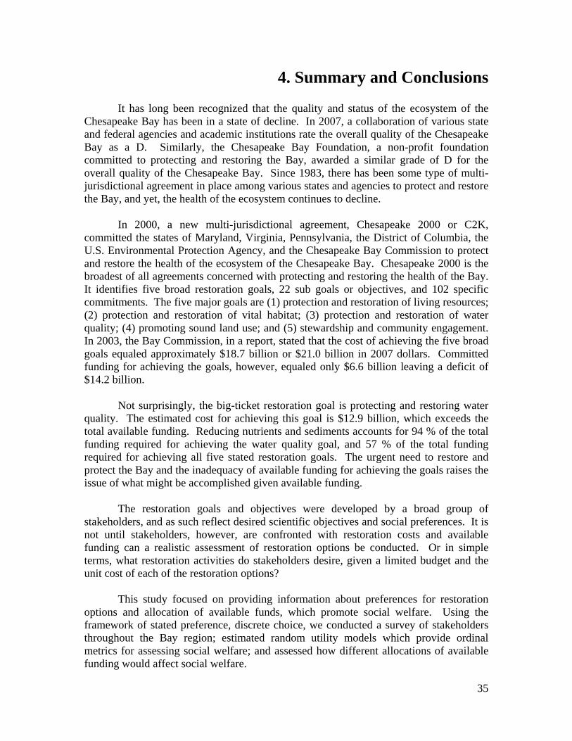
4. Summary and Conclusions

It has long been recognized that the quality and status of the ecosystem of the Chesapeake Bay has been in a state of decline. In 2007, a collaboration of various state and federal agencies and academic institutions rate the overall quality of the Chesapeake Bay as a D. Similarly, the Chesapeake Bay Foundation, a non-profit foundation committed to protecting and restoring the Bay, awarded a similar grade of D for the overall quality of the Chesapeake Bay. Since 1983, there has been some type of multi-jurisdictional agreement in place among various states and agencies to protect and restore the Bay, and yet, the health of the ecosystem continues to decline.

In 2000, a new multi-jurisdictional agreement, Chesapeake 2000 or C2K,

committed the states of Maryland, Virginia, Pennsylvania, the District of Columbia, the U.S. Environmental Protection Agency, and the Chesapeake Bay Commission to protect and restore the health of the ecosystem of the Chesapeake Bay. Chesapeake 2000 is the broadest of all agreements concerned with protecting and restoring the health of the Bay. It identifies five broad restoration goals, 22 sub goals or objectives, and 102 specific commitments. The five major goals are (1) protection and restoration of living resources; (2) protection and restoration of vital habitat; (3) protection and restoration of water quality; (4) promoting sound land use; and (5) stewardship and community engagement. In 2003, the Bay Commission, in a report, stated that the cost of achieving the five broad goals equaled approximately $18.7 billion or $21.0 billion in 2007 dollars. Committed funding for achieving the goals, however, equaled only $6.6 billion leaving a deficit of $14.2 billion.

Not surprisingly, the big-ticket restoration goal is protecting and restoring water

quality. The estimated cost for achieving this goal is $12.9 billion, which exceeds the total available funding. Reducing nutrients and sediments accounts for 94 % of the total funding required for achieving the water quality goal, and 57 % of the total funding required for achieving all five stated restoration goals. The urgent need to restore and protect the Bay and the inadequacy of available funding for achieving the goals raises the issue of what might be accomplished given available funding.

The restoration goals and objectives were developed by a broad group of

stakeholders, and as such reflect desired scientific objectives and social preferences. It is not until stakeholders, however, are confronted with restoration costs and available funding can a realistic assessment of restoration options be conducted. Or in simple terms, what restoration activities do stakeholders desire, given a limited budget and the unit cost of each of the restoration options?

This study focused on providing information about preferences for restoration

options and allocation of available funds, which promote social welfare. Using the framework of stated preference, discrete choice, we conducted a survey of stakeholders throughout the Bay region; estimated random utility models which provide ordinal metrics for assessing social welfare; and assessed how different allocations of available funding would affect social welfare.

35

Although C2K considers 22 sub-objectives or restoration categories, we included only six major restoration options: (1) restoration of oysters to stated target levels; (20 restoration of blue crabs to stated target levels; (3) restoration of shad; (4) restoration of wetlands; (5) reduction of nutrients and sediments; and (6) reduction of chemical contaminants. These six restoration options are viewed are being highly desired by stakeholders and account for 69.2 % of the total cost necessary for achieving all five broad restoration goals.

Our stated preference framework allowed us to determine preferences for not only

the six restoration options but also various levels of restoration targets (e.g., the restoration target for oysters is 10 times the level existing in 1994, which equals 11.2 million pounds of meats). Stakeholders were sent a questionnaire, which after asking some basic questions relating to Bay and regional issues, requested them to indicate their preferences for different mixes and levels of the six restoration options. Two of the restoration options included in the survey, however, may have caused some respondents to reject or, at least, assign a low preference to them. In earlier field tests of the survey questionnaire, we discovered that potential respondents did not have an adequate understanding of nutrient and sediment reductions and chemical contaminant reductions. We chose to use outputs used by monitoring agencies to reflect changes in these two options; these two outputs were beach closures for nutrient and sediment levels and seafood advisories for chemical contaminants.

Our sampling frame consisted of individuals who were well informed about Bay issues and problems in the region. Although we would have preferred to include more of the general public, funds were simply inadequate to do so. Also, our stakeholders were typically officers of associations or representatives of other large stakeholder groups. We did, however, include charter boat operators, watermen, fish processors, and scientists with the other stakeholders. In total, we had 15 stakeholder groups for the states of Maryland and Virginia. The survey was mailed to 1,500 stakeholders in the Bay region—750 each to Maryland and Virginia. Since some groups had only a few members, we had to resort to proportionate sampling of some groups and sampling of all members of other groups. In total, we received 299 responses to the 1,500 questionnaires mailed. The questionnaire included five questions. Four of the questions dealt with familiarity, importance, level of concern, and usage of the Bay, and the fifth question requested respondents to indicate their preference between two restoration bundles with different levels of restoration attributes. Two additional questions, identical to the fifth question were also included in the survey, but these two questions varied the levels of the restoration attributes. In addition, there was 15 versions of the survey instrument; all 15 versions were identical except they had varying levels of restoration options. Overall, we found stakeholders indicated a high level of importance to addressing improving education, reducing crime, decreasing air pollution, and restoring environmental quality to the Bay. There was little apparent concern among stakeholders for finding ways to reduce state taxes. We also found a very high proportion—66.1 %--

36

of the respondents indicated they believed they were very familiar with the Chesapeake Bay’s problems and issues. Somewhat surprising, however, was that a large majority of stakeholders indicated relatively low to moderate usage of the Bay. Last, 86.9 % of the respondents they were either very concerned or extremely concerned about the health of the Bay. Stakeholder responses to the questions about preferences for restoration options were used to estimate random utility models, which allowed us to determine an ordinal measure of utility as a function of the level of each of the restoration options. This random utility model or utility specification was then used in a mathematical programming specification to determine the budget allocations, which would generate the largest level of social welfare or satisfaction. The mathematical programming problem sought to determine the budget allocation, which maximized social welfare given budget constraints and per unit restoration costs. Several optimization problems were specified and solved, but in the conclusion we focus only on two solutions. The first solution is the maximization of utility in which the only constraint is the available funding, which equaled the funding--$2.6 billion-- committed to the six options considered in this study. This yields the allocation, which maximizes overall utility or welfare to society. The second problem considered the maximization of utility subject to the same budget constraint, but also constraints on the allowable levels of restoration options equal to the levels recommended by the Chesapeake Bay Commission as desired target levels. The solution to the first problem indicated that stakeholders desired levels of oysters and blue crabs well in excess of stated target levels. They preferred slightly lower levels of restoration of shad and wetlands than the target levels, and substantially lower levels of nutrient and chemical contaminant reductions. The solution to the second problem indicated a budget allocation, which would accomplish stated goals for oysters, blue crabs, shad, and wetlands, but would generate only modest reductions in chemical contaminants and nutrient levels. As is typical of many studies, this study does have several limitations. The first major limitation is that the outputs we used to specify the restoration options for nutrient and sediment reductions and chemical contaminant reductions may not have been well understood by the respondents. On the page preceding the question pertaining to preferences for restoration options, it was explained that beach advisories were being used as a measure of nutrient reduction and seafood advisories were being used as a measure of chemical contaminant reduction. It may be that individuals did not understand that nutrient and chemical reductions are necessary for achieve most of the restoration goals of the Bay. Alternatively, they have believed that nutrients really only affected beach usage and chemical contaminants only related to seafood advisories. Another major problem was the joint good nature of the options, particularly chemical contaminants and nutrient reductions. Reducing nutrients not only reduces beach closures, but it also helps the restoration of all living resources in the Bay. In addition, reductions in nutrients serve as inputs to the overall restoration process. Without careful

37

attention to the specification of outputs, the use of inputs as outputs could result in a double counting of the social welfare. Another problem we encountered was that many of the restoration options lack well defined targets and monitoring metrics, and thus, it was difficult to develop unit restoration cost for each of the options.

Despite the various problems, the analytical framework developed for this study provides powerful policy guidance on allocating limited funds to Bay restoration. We can ascertain that stakeholders prefer higher levels of restoration for oysters and blue crabs than specified by the restoration target levels. They also, however, prefer slightly lower levels of wetlands and shad than indicated by the target levels. They either desired considerably lower levels of nutrient and chemical contaminant reductions than the target levels, or stakeholders simply did not adequately understand the output metrics used to express nutrient and chemical contaminant reductions. Last, the analytical framework allows a more formal assessment of how changes in social welfare, budgets, and costs affect budget allocations, or of how different funding allocations might affect social welfare.

38

References

Chesapeake Bay Commission; the States of Maryland, Virginia, and Pennsylvania, the District of Columbia, and the United States of America. (2000). Chesapeake 2000.

Chesapeake Bay Commission. (2003). The Cost of a Clean Bay - Assessing Funding

Needs Throughout the Watershed. Available from the following web site: http://www.chesbay.state.va.us/.

Dillman, D.A. (2000). Mail and Internet Surveys: The Tailored Design Method. New

York: John Wiley & Sons. Hensher, D.A. and W.H. Greene. (2003). The Mixed Logit Model: The State of

Practice. Transportation Journal. Vol. 30, No. 2, pp. 133-176. Lancaster, K.J. (1966). A New approach to Consumer Theory. The Journal of Political

Economy. Vol. 74, No. 2, pp. 132-157. Lancaster, K.J. (1971). Consumer Demand: A New Approach. New York: Columbia

University Press. Mitchell, R.C. and R.C. Carson. (1989). Using Surveys to Value Public Goods: The

Contingent Valuation Method. Washington, D.C.: Resources for the Future. Washington, D.C.

Louviere, J.J., D.A. Hensher, and J.D. Swait. (2000). State Choice methods: Analysis

and Applications. Cambridge: Cambridge University Press. Bockstael, N.E. and K.E. McConnell (2007). Environmental and Resource Valuation

with Revealed Preferences: A Theoretical Guide to Empirical Models (The Economics of Non-Market Goods and Resources). Springer.

39

Appendix

40

41

42

43

44

45

46

47