assessing prognosis for chronic kidney...

ASSESSING PROGNOSIS FOR CHRONIC KIDNEY

DISEASE USING NEURAL NETWORKS

by

Michael R. Zeleny

B.S. Biology, Juniata College, 2012

Submitted to the Graduate Faculty of

the Graduate School of Public Health in partial fulfillment

of the requirements for the degree of

Master of Science

University of Pittsburgh

2016

UNIVERSITY OF PITTSBURGH

GRADUATE SCHOOL OF PUBLIC HEALTH

This thesis was presented

by

Michael R. Zeleny

It was defended on

April 22nd 2016

and approved by

Douglas Landsittel, PhD, Professor of Medicine, Biostatistics, and Clinical and Translational

Science, School of Medicine, University of Pittsburgh

Stewart J. Anderson, PhD, Professor of Biostatistics, Graduate School of Public Health,

University of Pittsburgh

Ada O. Youk, PhD, Associate Professor of Biostatistics, Epidemiology, and Clinical and

Translational Science, Graduate School of Public Health, School of Medicine, University of Pittsburgh

Thesis Advisor: Douglas Landsittel, PhD, Professor of Medicine, Biostatistics, and Clinical

and Translational Science, School of Medicine, University of Pittsburgh

ii

Copyright c© by Michael R. Zeleny

2016

iii

ASSESSING PROGNOSIS FOR CHRONIC KIDNEY DISEASE USING

NEURAL NETWORKS

Michael R. Zeleny, M.S.

University of Pittsburgh, 2016

Neural networks can be used as a potential way to predict continuous and binary outcomes.

With their ability to model complex non-linear relationships between variables and outcomes,

they may be better at prognosis than more traditional regression methods such as logistic

regression. In this thesis, the prognostic abilities of neural networks will be assessed using

data from the Consortium for Radiological Imaging Studies of Polycystic Kidney Disease

(CRISP) using clinically significant variables such as BMI, Blood Urea Nitrogen (BUN),

Height Adjusted Total Kidney Volume (htTKV), baseline estimated glomeruler filtration rate

(eGFR), and type of PKD.

Both a logisitic regression and variations of neural networks were modeled. The neural

networks had hidden units from 2 to 10, and weight decays from 0.01 to 0.05. Each of

these models was assessed by looking at Receiver Operator Characteristic (ROC) curves,

specifically the area under the curve (AUC). The complexity of these models was also looked

at by calculating the degrees of freedom for each model. More complex models could lead to

an overfitting of the data, and were therefore examined in this study.

The study showed that neural networks have the capability to predict the outcome of

stage 3 kidney disease better than a more traditional logistic regression, however, the models

become increasingly complex as the predictive ability increases.

These findings could have a great impact on public health in the future. They could

greatly impact the methods that are used for prognosis. The use of neural networks might

lead to better prognosis and earlier treatment for kidney disease based on an individuals

iv

Douglas Landsittel, PhD

ABSTRACT

baseline measurements of the aformentioned variables, or any other new biomarkers that are

discovered in the future.

v

TABLE OF CONTENTS

PREFACE . . . . . . . . . . . . . . . . . . . . . . . . . . . . . . . . . . . . . . . . . x

1.0 INTRODUCTION . . . . . . . . . . . . . . . . . . . . . . . . . . . . . . . . . 1

2.0 METHODS . . . . . . . . . . . . . . . . . . . . . . . . . . . . . . . . . . . . . 3

2.1 DATA AND VARIABLES . . . . . . . . . . . . . . . . . . . . . . . . . . . . 3

2.2 MULTIVARIABLE LOGISTIC REGRESSION . . . . . . . . . . . . . . . . 3

2.3 ARTIFICIAL NEURAL NETWORKS . . . . . . . . . . . . . . . . . . . . . 4

2.4 ROC CURVES . . . . . . . . . . . . . . . . . . . . . . . . . . . . . . . . . . 6

2.5 COMPLEXITY OF THE MODEL . . . . . . . . . . . . . . . . . . . . . . . 6

2.5.1 DEGREES OF FREEDOM FOR BINARY VARIABLES . . . . . . . 7

2.5.2 DEGREES OF FREEDOM FOR CONTINUOUS VARIABLES . . . 7

2.5.3 DEGREES OF FREEDOM FOR BOTH BINARY AND CONTINUOUS

VARIABLES . . . . . . . . . . . . . . . . . . . . . . . . . . . . . . . . 7

3.0 RESULTS . . . . . . . . . . . . . . . . . . . . . . . . . . . . . . . . . . . . . . 9

3.1 DESCRIPTION OF DATA . . . . . . . . . . . . . . . . . . . . . . . . . . . 9

3.2 MULTIVARIABLE LOGISTIC REGRESSION . . . . . . . . . . . . . . . . 10

3.3 NEURAL NETWORKS . . . . . . . . . . . . . . . . . . . . . . . . . . . . . 12

3.3.1 NEURAL NETWORKS WITH TWO HIDDEN UNITS . . . . . . . . 12

3.3.2 NEURAL NETWORKS WITH THREE HIDDEN UNITS . . . . . . . 14

3.3.3 NEURAL NETWORKS WITH FOUR HIDDEN UNITS . . . . . . . 16

3.3.4 NEURAL NETWORKS WITH FIVE HIDDEN UNITS . . . . . . . . 18

3.3.5 NEURAL NETWORKS WITH SIX HIDDEN UNITS . . . . . . . . . 20

3.3.6 NEURAL NETWORKS WITH SEVEN HIDDEN UNITS . . . . . . . 22

vi

3.3.7 NEURAL NETWORKS WITH EIGHT HIDDEN UNITS . . . . . . . 24

3.3.8 NEURAL NETWORKS WITH NINE HIDDEN UNITS . . . . . . . . 26

3.3.9 NEURAL NETWORKS WITH TEN HIDDEN UNITS . . . . . . . . 28

3.4 SUMMARY OF MODEL COMPLEXITY . . . . . . . . . . . . . . . . . . . 30

4.0 DISCUSSION . . . . . . . . . . . . . . . . . . . . . . . . . . . . . . . . . . . . 32

APPENDIX. R CODE . . . . . . . . . . . . . . . . . . . . . . . . . . . . . . . . . 34

BIBLIOGRAPHY . . . . . . . . . . . . . . . . . . . . . . . . . . . . . . . . . . . . 46

vii

LIST OF TABLES

1 Descriptive Statistics for Continuous Variables . . . . . . . . . . . . . . . . . 9

2 Descriptive Statistics for Continuous Variables . . . . . . . . . . . . . . . . . 10

3 Multivariable Logistic Regression . . . . . . . . . . . . . . . . . . . . . . . . . 11

4 AUC Values for Neural Networks with Two Hidden Units . . . . . . . . . . . 14

5 AUC Values for Neural Networks with Three Hidden Units . . . . . . . . . . 16

6 AUC Values for Neural Networks with Four Hidden Units . . . . . . . . . . . 18

7 AUC Values for Neural Networks with Five Hidden Units . . . . . . . . . . . 20

8 AUC Values for Neural Networks with Six Hidden Units . . . . . . . . . . . . 22

9 AUC Values for Neural Networks with Seven Hidden Units . . . . . . . . . . 24

10 AUC Values for Neural Networks with Eight Hidden Units . . . . . . . . . . . 26

11 AUC Values for Neural Networks with Nine Hidden Units . . . . . . . . . . . 28

12 AUC Values for Neural Networks with Ten Hidden Units . . . . . . . . . . . 30

13 Summary of Model Complexity . . . . . . . . . . . . . . . . . . . . . . . . . . 30

viii

LIST OF FIGURES

1 Diagram of Simple Neural Network . . . . . . . . . . . . . . . . . . . . . . . . 5

2 ROC Curve for Multivariable Logistic Regression . . . . . . . . . . . . . . . . 12

3 ROC Curves for Neural Networks with Two Hidden Units . . . . . . . . . . . 13

4 ROC Curves for Neural Networks with Three Hidden Units . . . . . . . . . . 15

5 ROC Curves for Neural Networks with Four Hidden Units . . . . . . . . . . . 17

6 ROC Curves for Neural Networks with Five Hidden Units . . . . . . . . . . . 19

7 ROC Curves for Neural Networks with Six Hidden Units . . . . . . . . . . . . 21

8 ROC Curves for Neural Networks with Seven Hidden Units . . . . . . . . . . 23

9 ROC Curves for Neural Networks with Eight Hidden Units . . . . . . . . . . 25

10 ROC Curves for Neural Networks with Nine Hidden Units . . . . . . . . . . . 27

11 ROC Curves for Neural Networks with Ten Hidden Units . . . . . . . . . . . 29

ix

PREFACE

I would like to express my thanks and gratitude to Dr. Douglas Landsittel, who brought this

topic to my attention and lead me throughout the entire learning process for this thesis. I

would also like to thank both Dr. Stewart J. Anderson and Dr. Ada O. Youk for sitting on

my thesis committee and giving me important suggestions to succeed in this thesis.

I would also like to thank my family, especially my parents Robin and Ray Zeleny for

pushing me to achieve this degree and supporting me throughout the process. They have

always pushed me to be my best.

x

1.0 INTRODUCTION

Polycystic kidney disease (PKD) is a group of disorders that result in renal cyst development.

PKD is one of the leading causes of end stage renal failure. Most forms of the disease are

inherited although it is possible to develop the disease in other ways. Of the hereditary types

of PKD, the PKD1 genotype accounts for about 85% of PKD cases. PKD2 is another less

common genotype1. The significance of PKD in leading to renal failure strongly motivates

the need to study prognostic factors for renal decline within this population.

One way to determine if an individual has chronic kidney disease (CKD) is by measuring

glomerular filtration rate (GFR). The GFR can be estimated in a number of ways including

serum-creatinine based estimates, which can be based on Cockcroft-Gault equations, Mod-

ification of Diet in Renal Disease, or the CKD-EPI equation that uses information from

demographics and measured values of serum-creatinine2. It has been found that the CKD-EPI

equation results in a more accurate prediction of GFR than the MDRD estimate3.

The estimation of GFR is used for diagnosing stage 3 kidney disease. When looking at a

value of GFR, the larger the number indicates better functioning of the kidney. When the

GFR value drops below a threshold value of 60mL/min1.73m2 the individual is classified as having

stage 3 kidney disease, which is considered chronic kidney disease. At this point half of the

normal adult kidney function is lost4.

There are many variables which can be used as potential predictors to predict stage

3 kidney disease. One measure that could be a potential predictor of the onset of kidney

disease is the total kidney volume, which can be measured as height adjusted total kidney

volume. In one study, it was found that a height adjusted total kidney volume (htTKV)

600 ccm

was a significant predictor of developing renal sufficiency in PKD patients5. Blood

urea nitrogen (BUN) levels can also indicate the onset of kidney disease with higher BUN

1

concentrations indicating advancement of disease in the kidney6. Body Mass Index (BMI)

can also be considered a potential predictor as one study showed that study participants who

developed kidney disease had a higher mean BMI than those who did not develop kidney

disease7.

The Consortium for Radiological Imaging Studies of Polycystic Kidney Disease (CRISP)

was established to use imaging techniques to determine if certain markers, such as the

ones above, can be used to determine the progression of kidney disease in a cohort of

individuals. Individuals enrolled in the CRISP study had some form of PKD and were

followed prospectively8. Measurements of different variables were obtained to determine if

there was any significance between possible markers and stage 3 kidney disease.

Neural networks, with the potential predictors mentioned, can be explored as a classifi-

cation technique alongside a more traditional logistic regression approach to determine the

predictive ability of each different model in turn. Neural networks allow for the modelling of

complex non-linear relationships through the use of a component called the hidden layer, and

in some studies show better predictive performance than techniques such as logistic regression9.

When non-linear relationships are present the network will automatically adjust its weights in

order to reflect this, a feature not present in traditional logistic regression. Neural networks,

because of this ability to utilize non-linear relationships and complex interactions, are prone

to overfitting. Weight decay is one way to address this problem with neural networks as it

penalizes large weight terms to reduce complexity of the model10.

In this thesis, we will assess whether neural networks can improve on the prognostic

ability of logistic models specific to the CRISP study and CKD outcomes. We will also assess

the utility of different variations of network model fitting for these data. The prognostic

ability of neural networks will be assessed and compared to prognostic abilities of logistic

regression to analyze binary outcomes. When examining neural network prognostic abilities,

models with different number of hidden layers will be assessed and overfitting considerations

will be assessed by using different values of weight decay. Model complexity using degrees of

freedom will also be assessed in relation to prognostic abilities.

2

2.0 METHODS

2.1 DATA AND VARIABLES

In this study, data from CRISP was used to develop a predictive model for the outcome of

chronic kidney disease. For purposes of this analysis, the glomerular filtration rate (GFR),

as estimated by the CKD-EPI equations (i.e. eGFR), was categorized as either eGFR of

<60mL/min1.73m2 i.e. reached Stage 3 CKD, or eGFR ≥60mL/min

1.73m2 . Participants who reached CKD

Stage 3 or worse at any time during through the study were categorized as having the event

of Stage 3 kidney disease (even if they were lost to follow-up because renal function can

only decline over time). Participants who had an eGFR ≥60mL/min1.73m2 at 10 years or more past

baseline were categorized as no event. Participants who had no available eGFR measurements

at 10 years or more past baseline were excluded from the analysis.

The predictor variables of interest for this study were height adjusted total kidney volume

(htTKV), eGFR at baseline, body mass index (BMI), Blood Urea Nitrogen (BUN), and their

genotype of PKD (i.e. PKD1, PDK2, and no mutation detected, or NMD). For this study,

PKD2 and NMD were grouped together as the reference category.

2.2 MULTIVARIABLE LOGISTIC REGRESSION

Multivariable logistic regression was used to predict the outcome that a patient would reach

stage three kidney disease in the duration of the study. The model for this logistic regression

3

was defined as follows:

ln(p

1− p) = Xβ (2.1)

Where X is the matrix of covariates used in this study and β is the vector of parameters

estimated through maximum likelihood estimation. When constructing this model, the

variables used were based on clinical significance. In this case, the predictor variables used to

build the model were BUN, PKD type, BMI, eGFR, and htTKV, and the outcome variable

was an indicator of type 3 kidney disease (CKD).

2.3 ARTIFICIAL NEURAL NETWORKS

Feed forward neural networks with a single hidden layer were also used to model the data

with the clinically significant variables (named a-priori). Feed forward neural networks do

not form a cycle and are diagramed in Figure 1. To describe the model, we use the following

notation:

1. Xik: i=1,2,. . .,r, k=1,2,. . . ,n where i corresponds to each input, in this case variables and

k corresponds to each observation

2. Wij: i=1,2,. . .,r j=1,2,,h defined as weights, where i corresponds to the weight for each

input and j corresponding to the hidden unit number in which the data feeds to

3. Hj : j=1,2,. . .,h corresponding to hidden units, where j corresponds to hidden unit number

4. Vj: j=1,2,. . .,h corresponding to weights, where j corresponds to the hidden unit number

5. W0j: intercept term

6. V0j: intercept term

7. Y: outcome

Model coeffiecients are fit by minimizing the log likelihood of the data using an iterative

process called back propogation, where coefficients are adjusted in small steps until they

reach a local minimum. Feed forward neural networks can essentially be thought of as a set

of nested logistic models, as shown in Figure 1. For this study 1000 iterations were used.

4

Figure 1: Diagram of Simple Neural Network

Each of the hj’s are referred to as hidden units. The network can have any number of

hidden units or hidden layers. The final output, or predicted response, with a single hidden

layer, is given by equation 2.2 for the kth observation .

yk = f(v0 +H∑j=1

vjf{w0j +

p∑i=1

wijxik}) (2.2)

Weight decay, which is a penalty term that is multiplied by the sum of squared weights

was also used to minimize over-fitting and optimize model convergence. This penalizes larger

weights more and the backpropogation algorithm minimizes the error using these penalized

weights, rather than unpenalized weights. The weight decay values in this thesis were varied

from 0.01 to 0.05.

5

A neural network may have a number of hidden layers. In this study, one hidden layer was

used and the number of hidden units in this hidden layer was allowed to vary. The number of

hidden units chosen were 2 through 10 for the hidden layer. Based on these different numbers

of hidden units, the predictive ability of each network was assessed.

2.4 ROC CURVES

Receiver Operating Characteristic (ROC) curves graph the sensitivity (y-axis) by 1-sensitivity

(x-axis). Each specific cutoff value yields a different sensitivity and specificity for model

prediction13.

sensitivity =TruePositives

TruePositives+ FalseNegatives(2.3)

specificity =TrueNegatives

TrueNegatives+ FalsePositives(2.4)

We will also calculate he AUC, which is the probability that the classifier will rank a

randomly chosen positive instance higher than a randomly chosen negative instance14. The

values of these AUCs will be assessed in this study and confidence intervals will be calculated.

2.5 COMPLEXITY OF THE MODEL

The effect of weight decay and number of hidden units on the complexity of the model

was also of interest. To determine the complexity of the model, a calculation was used to

determine the number of degrees of freedom there were for each of the neural networks

tested. An estimate of the degrees of freedom was used based on both degrees of freedom

calculations for binary variables and degrees of freedom calculations for continuous variables

proposed by Landsittel (2009)15. Landsittel calculated the mean likelihood ratio test for

model independence and associates that mean with degrees of freedom (df) for the associated

6

chi-squared distribution, and derived equations for interpolating the degrees of freedom over

a range of models.

2.5.1 DEGREES OF FREEDOM FOR BINARY VARIABLES

For binary variables the degrees of freedom calculation relies on both the maximum number

of terms, given by 2i - 1 where i corresponds to the number of variables, and the number

of model parameters, given by h(i + 1) + (h + 1), where h is the number of hidden units.

Using these values, the degrees of freedom can be calculated using the interpolated equation

dfp

= 0.6643 + 0.1429× log2(m− p), where m is the maximum number of terms and p is the

number of model parameters.

2.5.2 DEGREES OF FREEDOM FOR CONTINUOUS VARIABLES

For continuous variables the degrees of freedom calculation relies on the number of hidden

units, h, and the number of variables, i. Using these values, the degrees of freedom can be

calculated using the interpolated equation df = h× [3× (i− 2) + 5].

2.5.3 DEGREES OF FREEDOM FOR BOTH BINARY AND CONTINUOUS

VARIABLES

No established methods exist to calculate degrees of freedom for both binary and continuous

variables in the same model. Therefore estimation of the degrees of freedom for these models

was accomplished by the following steps:

1. Let i be the number of variables in the model

2. Let ib be the number of binary variables in the model

3. Let ic be the number of continuous variables in the model

4. Let propb be the proportion of binary variables in the model, ibi

and propc be the proportion

of continuous variables in the model, 1− propb

7

5. Determine the degrees of freedom if all i variables were binary variables

6. Determine the degrees of freedom if all i variables were continuous variables

7. Estimate model degrees of freedom using propb × dfb + propc × dfc

The above method was used for each of neural network models. This method assumes the

degrees of freedom varies proportionally between what it would be with all binary variables

versus all continuous variables. Future studies will need to validate this approach.

8

3.0 RESULTS

3.1 DESCRIPTION OF DATA

In this section we report the results of the analysis performed in the thesis. There were a

total of 241 patients who were examined for the presence of stage 3 kidney disease. Of these,

203 patients had complete data for the variables of interest and 38 patients had incomplete

data for these variables. Of the 38 patients with missing data, 33 were missing the outcome

variable,that is, Stage 3 kidney Disease. Patients with missing data were dropped for this

analysis.

Table 1: Descriptive Statistics for Continuous Variables

Variable Mean (Std. Dev)

Estimated GFR 91.57 (22.94)

BMI 25.96 (5.28)

Height Adjusted Total Kidney Volume 637.47(377.98)

BUN 14.59(4.30)

9

On the set of complete data, descriptive statistics were calculated. From Table 1, the

mean estimated GFR was 91.57 with a standard deviation of 22.94. This mean puts the

average patient into the category of no Stage 3 kidney disease. The average BMI of the

patients was 25.96 with a standard deviation of 5.28. The mean height adjusted total kidney

volume was 637.47 with a standard deviation of 377.98. The average BUN of the patients

was 14.59 with a standard deviation of 4.30.

Table 2: Descriptive Statistics for Continuous Variables

Variable Total (%) (N=203)

Stage 3 Kidney Disease Yes 123(61%)

No 80(39%)

Type of PKD PKD1 162(80%)

Other 41(20%)

From Table 2 of the patients in the study, 123 were diagnosed with stage 3 kidney disease

(61%) and 80 did not reach stage 3 kidney disease during the course of the study (39%). Out

of the patients that were in the study who suffer from PKD, 162 of them have PKD1 (80%),

whereas only 41 have PKD2 or another classification of the disease (20%).

3.2 MULTIVARIABLE LOGISTIC REGRESSION

A multivariable logistic regression was run with the clinically significant variables mentioned

in Section 1.

10

Table 3: Multivariable Logistic Regression

Variable Odds Ratio p-value

eGFR 0.9424 <0.00001

Type of PKD 1.976 0.1578

Height Adjusted TKV 1.004 <0.0001

BMI 1.029 0.4838

BUN 1.130 0.0476

Table 3 shows the results of the multivariable logistic regression. Height adjusted total

kidney volume and the estimated GFR were the most significant predictors with BUN also

being significant at the 0.05 level. Type of PKD and BMI were not statistically significance

based on these data, but were left in the model because they were deemed to be clinically

significant.

11

Figure 2: ROC Curve for Multivariable Logistic Regression

The ROC curve was also plotted for the multivariable logistic regression and the area

under the curve was calculated. As seen from Figure 1 the discrimination exhibited by the

multivariable logistic regression is excellent with an AUC of 0.906.

3.3 NEURAL NETWORKS

3.3.1 NEURAL NETWORKS WITH TWO HIDDEN UNITS

Feedforward neural networks were constructed with a single hidden layer in which the number

of hidden units was 2. These neural networks were then varied with multiple values of weight

decay to explore how weight decays affect the predictive abilities of these networks.

12

Figure 3: ROC Curves for Neural Networks with Two Hidden Units

From Figure 3, the AUCs of the ROC curves for these neural networks have a maximum

value of 0.913 when weight decay of 0.05 is used. The minimum value of the AUC for this set

of neural networks is 0.859 when the weight decay was set to 0.01. The other weight decay

values gave values of 0.889, 0.911, and 0.911, for weight decay values of 0.02, 0.03, and 0.04

respectively. These results are summarized below in Table 4.

13

Table 4: AUC Values for Neural Networks with Two Hidden Units

Weight Decay AUC 95% Confidence Interval

0.01 0.859 (0.804,0.914)

0.02 0.889 (0.843,0.935)

0.03 0.911 (0.868,0.954)

0.04 0.911 (0.867,0.955)

0.05 0.913 (0.870,0.956)

For neural networks with two hidden units the confidence intervals were reasonably narrow

with widths ranging from ±0.043 to ±0.055.

3.3.2 NEURAL NETWORKS WITH THREE HIDDEN UNITS

Feedforward neural networks were again constructed with a single hidden layer in which the

number of hidden units was 3. These neural networks were then varied with multiple values

of weight decay to again explore how weight decays affect the predictive abilities of these

networks.

14

Figure 4: ROC Curves for Neural Networks with Three Hidden Units


value of 0.940 when weight decays of 0.01 and 0.03 are used. The minimum value of the AUC

for this set of neural networks is 0.911 when the weight decay was set to 0.04. The other

weight decay values gave values of 0.916 and 0.928, for weight decay values of 0.02 and 0.05

respectively. These results are summarized in Table 5 below.

15

Table 5: AUC Values for Neural Networks with Three Hidden Units


0.01 0.940 (0.906,0.973)

0.02 0.916 (0.878,0.953)

0.03 0.911 (0.868,0.954)

0.04 0.911 (0.867,0.954)

0.05 0.928 (0.893,0.963)

For neural networks with three hidden units the confidence intervals were reasonably

narrow with widths ranging from ±0.034 to ±0.038.

3.3.3 NEURAL NETWORKS WITH FOUR HIDDEN UNITS




networks.

16

Figure 5: ROC Curves for Neural Networks with Four Hidden Units






17

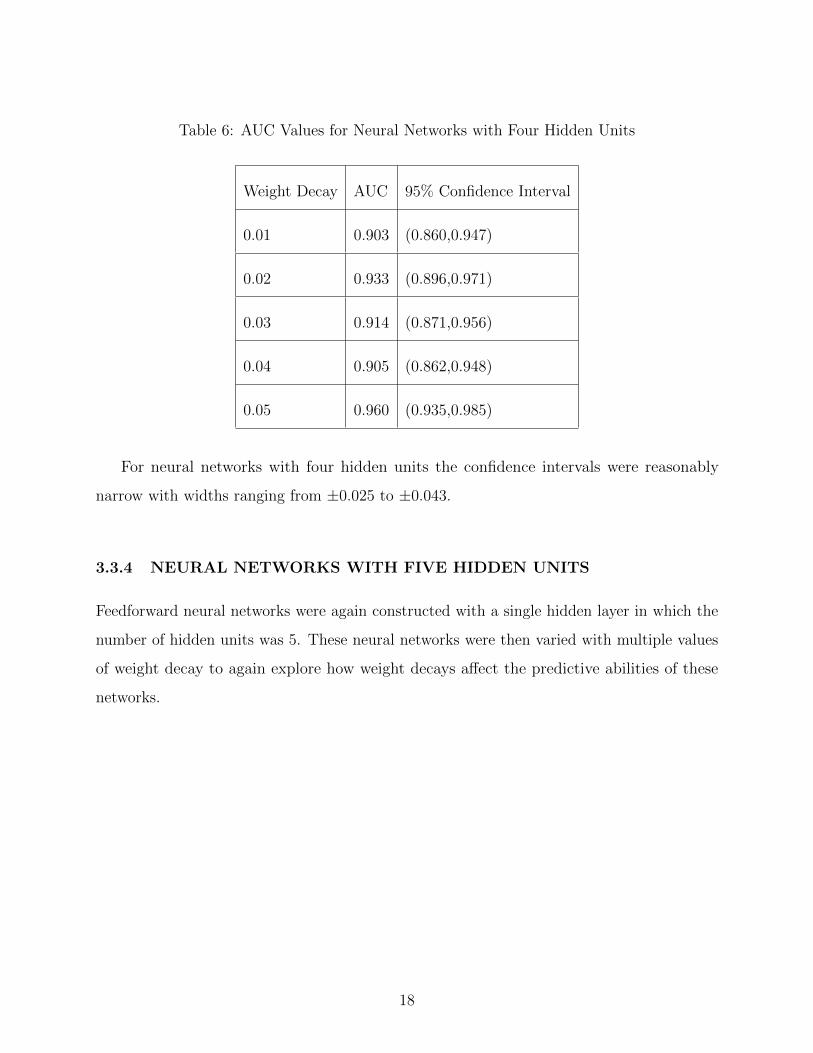
Table 6: AUC Values for Neural Networks with Four Hidden Units


0.01 0.903 (0.860,0.947)

0.02 0.933 (0.896,0.971)

0.03 0.914 (0.871,0.956)

0.04 0.905 (0.862,0.948)

0.05 0.960 (0.935,0.985)

For neural networks with four hidden units the confidence intervals were reasonably


3.3.4 NEURAL NETWORKS WITH FIVE HIDDEN UNITS




networks.

18

Figure 6: ROC Curves for Neural Networks with Five Hidden Units






19

Table 7: AUC Values for Neural Networks with Five Hidden Units


0.01 0.902 (0.858,0.946)

0.02 0.937 (0.903,0.970)

0.03 0.912 (0.869,0.955)

0.04 0.926 (0.888,0.964)

0.05 0.942 (0.911,0.973)

For neural networks with five hidden units the confidence intervals were reasonably narrow


3.3.5 NEURAL NETWORKS WITH SIX HIDDEN UNITS




networks.

20

Figure 7: ROC Curves for Neural Networks with Six Hidden Units


value of 0.960 when weight decay of 0.05 is used. The minimum value of the AUC for this

set of neural networks is 0.924 when the weight decay was set to 0.01 and 0.03. The other

weight decay values gave values of 0.947 and 0.952, for weight decay values of 0.02 and 0.04


21

Table 8: AUC Values for Neural Networks with Six Hidden Units


0.01 0.924 (0.884,0.964)

0.02 0.947 (0.919,0.975)

0.03 0.924 (0.884,0.964)

0.04 0.952 (0.925,0.978)

0.05 0.960 (0.936,0.984)

For neural networks with six hidden units the confidence intervals were reasonably narrow


3.3.6 NEURAL NETWORKS WITH SEVEN HIDDEN UNITS




networks.

22

Figure 8: ROC Curves for Neural Networks with Seven Hidden Units




values gave values of 0.951, 0.946, and 0.942, for weight decay values of 0.01, 0.02 and 0.05


23

Table 9: AUC Values for Neural Networks with Seven Hidden Units


0.01 0.951 (0.924,0.978)

0.02 0.9465 (0.915,0.976)

0.03 0.820 (0.761,0.879)

0.04 0.967 (0.945,0.988)

0.05 0.942 (0.912,0.971)

For neural networks with seven hidden units the confidence intervals were reasonably


3.3.7 NEURAL NETWORKS WITH EIGHT HIDDEN UNITS




networks.

24

Figure 9: ROC Curves for Neural Networks with Eight Hidden Units






25

Table 10: AUC Values for Neural Networks with Eight Hidden Units


0.01 0.949 (0.920,0.979)

0.02 0.939 (0.908,0.970)

0.03 0.940 (0.911,0.969)

0.04 0.938 (0.904,0.973)

0.05 0.977 (0.959,0.996)

For neural networks with eight hidden units the confidence intervals were reasonably


3.3.8 NEURAL NETWORKS WITH NINE HIDDEN UNITS




networks.

26

Figure 10: ROC Curves for Neural Networks with Nine Hidden Units






27

Table 11: AUC Values for Neural Networks with Nine Hidden Units


0.01 0.984 (0.971,0.996)

0.02 0.930 (0.898,0.963)

0.03 0.968 (0.944,0.993)

0.04 0.969 (0.948,0.990)

0.05 0.965 (0.944,0.986)

For neural networks with nine hidden units the confidence intervals were reasonably


3.3.9 NEURAL NETWORKS WITH TEN HIDDEN UNITS




networks.

28

Figure 11: ROC Curves for Neural Networks with Ten Hidden Units






29

Table 12: AUC Values for Neural Networks with Ten Hidden Units


0.01 0.980 (0.967,0.994)

0.02 0.988 (0.976,1.000)

0.03 0.981 (0.966,0.997)

0.04 0.929 (0.894,0.963)

0.05 0.983 (0.969,0.997)

For neural networks with two hidden units the confidence intervals were reasonably narrow


3.4 SUMMARY OF MODEL COMPLEXITY

Degrees of freedom were estimated for neural networks with 2, 4, 6, 8, and 10 hidden units

and a weight decay value of 0.01 to determine the model complexity.

Table 13: Summary of Model Complexity

Method Hidden Units Weight Decay AUC 95% CI Parameters df AIC

Logistic - - 0.906 (0.863,0.949) 5 5 165.84

NN 2 0.01 0.859 (0.804,0.914) 15 26.11 125.66

NN 4 0.01 0.903 (0.860,0.947) 29 49.48 160.10

NN 6 0.01 0.924 (0.884,0.964) 43 73.40 202.33

NN 8 0.01 0.949 (0.920,0.979) 57 95.8 240.01

NN 10 0.01 0.980 (0.967,0.994) 71 118.2 263.24

30

From Table 13, as the number of hidden units is increased in the model the degrees of

freedom also increases. The maximum degrees of freedom calculated for this study were

118.20 when the number of hidden units was set to 10 and the minimum degrees of freedom

calculated were 26.11 when the number of hidden units were set to 2. Table 13 also shows

that as the number of hidden units increases the AIC value also increases with the maximum

being 263.24 for a neural network with 10 hidden units and a minimum being 125.66 for a

neural network with 2 hidden units. The logistic regression had a lower value for degrees of

freedom and also had a lower AIC value than all but neural networks with 2 and 4 degrees of

freedom.

31

4.0 DISCUSSION

When looking at the prediction of Stage 3 kidney disease, it has been shown that neural

networks can perform better than standard logistic regression using the same variables. The

maximum AUC value found in this study was 0.988 with a confidence interval of (0.976,

1.000) whereas the logistic regression gave an AUC of 0.904 with a confidence interval of

(0.863, 0.949).

With new research being completed, new biomarkers and other potential predictors are

being identified. With these new potential predictors being identified, the importance of

prediction modeling becomes highlighted. Prediction models have the ability to both provide

the ability to assess predictors in a model and the ability to estimate risk for individual

patients16. Neural networks can potentially more accurately predict the risk of an individual

to develop a certain disease and therefore allow for better medical treatment and prevention.

This has already been shown in prediction of prostate cancer, where neural networks could

be used in order to change the way patients are counseled for treatment options17.

The research to identify new biomarkers extends into the field of nephrology where both

the PKD Foundation18 and the Consortium for Radiologic Imaging Studies of Polycystic

Kidney Disease8 are both working to identify new markers. Once new markers are identified,

neural networks will be able to use these markers to make predictions on outcome predictions

and potentially change the way treatments are administered based on baseline values of

biomarkers.

However, when looking at modern regression techniques such as neural networks the pros

and cons must be weighed. Neural networks allow for the modeling of complex non-linear

relationships between variables, detection of all possible interactions between variables, and

32

can be used with many different algorithms for training for specific types of data. All of these

could be very useful when employed for prediction modeling. Neural networks have certain

disadvantages as well. These disadvantages include the use of neural networks as a black box

technique, leading to a limited ability for detecting casual relationships between variables

and hence, making interpretation difficult. Neural networks are also prone to overfitting.

However, to adress overfitting, weight decay can be used. Limiting the amount of training

can also be a solution to overfitting. For looking at outcome prediction, neural networks are

a good candidate for prediction modeling.

Overall, the use of neural networks is a promising technique in which known predictors

and biomarkers can be used in order to create a prediction model. And with this prediction

model, the way in which the condition is treated could be modified in a way that benefits

patients with the disease.

33

APPENDIX

R CODE

##Libraries

require(mlogit)

require(nnet)

require(psych)

require(ROCR)

library(pROC)

##Data management

summary(thesis.data)

thesis <-cbind(thesis.data$ckd_epi , thesis.data$type , thesis.data$httkv0 , thesis.data$bmi_c0, thesis.data$sbune_ca0 , thesis.data$ckd3_120)

colnames(thesis)<-c("ckd_epi","type","httkv0","bmi","sbun","ckd3")

describe(thesis)

thesis.f<-data.frame(thesis)

thesis.final <-na.omit(thesis.f)

## Descriptives

describe(thesis.final)

summary(thesis.final)

t=table(thesis.final$type)

tcount=as.data.frame(t)

tcount

o=table(thesis.final$ckd3)

ocount=as.data.frame(o)

ocount

# multivariable logistic regression

full <-glm(ckd3~ckd_epi+type+httkv0+bmi+sbun , family=binomial(link=logit),data=thesis.final)

summary(full)

pred1 <-predict(full , type=c("response"))

thesis.final$pred1=pred1

34

logisticROC <-roc(ckd3~pred1 , data=thesis.final , plot=TRUE , print.auc=TRUE , legacy.axes=T, main="ROC Curve for Logistic Regression", ci=T)

#seed

set.seed (0625199016)

#2 Hidden Unit Network Variations

#neural network with 2 hidden units with weight decay 0.01

neural1 <-nnet(ckd3~ckd_epi+bmi+type+httkv0+sbun ,data=thesis.final ,size=2, entropy=TRUE , maxit =1000, decay =0.01)

summary(neural1)

pred21 <-predict(neural1 , newdata=thesis.final , type=c("raw"))


n21 <-roc(ckd3~pred2 , data=thesis.final , print.auc=T, legacy.axes=T, plot=T, main="2 Hidden Units and Weight Decay of 0.01")

plot(n21)

#neural network with 2 hidden units with weight decay 0.02

neural12 <-nnet(ckd3~ckd_epi+bmi+type+httkv0+sbun ,data=thesis.final ,size=2, entropy=TRUE , maxit =1000 , decay =0.02)

summary(neural12)



n22 <-roc(ckd3~pred22 , data=thesis.final , print.auc=T, legacy.axes=T, plot=T, main="2 Hidden Units and Weight Decay of 0.02")

plot(n22)

##neural network with 2 hidden units with weight decay 0.03


summary(neural13)



n23 <-roc(ckd3~pred23 , data=thesis.final , print.auc=T, legacy.axes=T, plot=T, main="2 Hidden Units and Weight Decay 0.03")

plot(n23)



summary(neural14)



n24 <-roc(ckd3~pred24 , data=thesis.final , print.auc=T, plot=T, legacy.axes=T, main="2 Hidden Units and Weight Decay of 0.04")

plot(n24)



summary(neural15)




plot(n25)

##plots for 2 Hidden units

35

par(mfrow=c(3,2))

n21 <-roc(ckd3~pred21 , data=thesis.final , print.auc=T, legacy.axes=T, plot=T, main="A. Weight Decay of 0.01", ci=F)

n22 <-roc(ckd3~pred22 , data=thesis.final , print.auc=T, legacy.axes=T, plot=T, main="B. Weight Decay of 0.02", ci=F)

n23 <-roc(ckd3~pred23 , data=thesis.final , print.auc=T, legacy.axes=T, plot=T, main="C. Weight Decay of 0.03", ci=F)

n24 <-roc(ckd3~pred24 , data=thesis.final , print.auc=T, plot=T, legacy.axes=T, main="D. Weight Decay of 0.04", ci=F)

n25 <-roc(ckd3~pred25 , data=thesis.final , print.auc=T, plot=T, legacy.axes=T, main="E. Weight Decay of 0.05", ci=F)

par(mfrow=c(1,1))

##CI can be toggled to T to obtain confidence interval



summary(neural21)



n31 <-roc(ckd3~pred31 , data=thesis.final , print.auc=T, plot=T, legacy.axes=T, main="3 Hidden Units and Weight Decay 0.01")

plot(n31)



summary(neural22)




plot(n32)



summary(neural23)




plot(n33)



summary(neural24)



n34 <-roc(ckd3~pred34 , data=thesis.final ,print.auc=T, plot=T, legacy.axes=T, main="3 Hidden Units and Weight Decay 0.04")

plot(n34)



summary(neural25)




plot(n35)

36

##plots 3 Hidden Units

par(mfrow=c(3,2))

n31 <-roc(ckd3~pred31 , data=thesis.final , print.auc=T, plot=T, legacy.axes=T, main="A. Weight Decay 0.01", ci=F)

n32 <-roc(ckd3~pred32 , data=thesis.final , print.auc=T, plot=T, legacy.axes=T, main="B. Weight Decay 0.02", ci=F)

n33 <-roc(ckd3~pred33 , data=thesis.final , print.auc=T, plot=T, legacy.axes=T, main="C. Weight Decay 0.03", ci=F)

n34 <-roc(ckd3~pred34 , data=thesis.final , print.auc=T, plot=T, legacy.axes=T, main="D. Weight Decay 0.04", ci=F)

n35 <-roc(ckd3~pred35 , data=thesis.final , print.auc=T, plot=T, legacy.axes=T, main="E. Weight Decay 0.05", ci=F)

par(mfrow=c(1,1))



summary(neural31)



n41 <-roc(ckd3~pred41 , data=thesis.final ,print.auc=T, plot=T, legacy.axes=T, main="4 Hidden Units and Weight Decay 0.01")

plot(n41)



summary(neural32)




plot(n42)



summary(neural33)




plot(n43)



summary(neural34)




plot(n44)



summary(neural35)




37

plot(n45)

##plot 4 Hidden Units

par(mfrow=c(3,2))






par(mfrow=c(1,1))



summary(neural41)




plot(n51)



summary(neural42)



n52 <-roc(ckd3~pred52 , data=thesis.final , print.auc=T,plot=T, legacy.axes=T, main="5 Hidden Units and Weight Decay 0.02")

plot(n52)



summary(neural43)




plot(n53)



summary(neural44)




plot(n54)



summary(neural45)




38

plot(n55)


par(mfrow=c(3,2))






par(mfrow=c(1,1))



summary(neural51)




plot(n61)



summary(neural52)




plot(n62)



summary(neural53)




plot(n63)



summary(neural54)



n64 <-roc(ckd3~pred64 , data=thesis.final , print.auc=T, plot=T, legacy.axes=T, main="6 Hidden Units and Weight Deacy 0.04")

plot(n64)



summary(neural55)



39


plot(n65)


par(mfrow=c(3,2))




n64 <-roc(ckd3~pred64 , data=thesis.final , print.auc=T, plot=T, legacy.axes=T, main="D. Weight Deacy 0.04", ci=F)


par(mfrow=c(1,1))



summary(neural61)




plot(n71)



summary(neural62)




plot(n72)



summary(neural63)




plot(n73)



summary(neural64)




plot(n74)



summary(neural65)


40



plot(n75)


par(mfrow=c(3,2))






par(mfrow=c(1,1))



summary(neural71)




plot(n81)



summary(neural72)




plot(n82)



summary(neural73)




plot(n83)



summary(neural74)



n84 <-roc(ckd3~pred84 , data=thesis.final , print.auc=T, plot=t, legacy.axes=T, main="8 Hidden Units and Weight Decay 0.04")

plot(n84)



summary(neural75)

41




plot(n85)


par(mfrow=c(3,2))




n84 <-roc(ckd3~pred84 , data=thesis.final , print.auc=T, plot=t, legacy.axes=T, main="D. Weight Decay 0.04", ci=F)


par(mfrow=c(1,1))



summary(neural81)




plot(n91)



summary(neural82)




plot(n92)



summary(neural83)




plot(n93)



summary(neural84)




plot(n94)



42

summary(neural85)




plot(n95)

##plots for 9 Hidden Units

par(mfrow=c(3,2))






par(mfrow=c(1,1))



summary(neural91)




plot(n101)



summary(neural92)




plot(n102)



summary(neural93)




plot(n103)



summary(neural94)




plot(n104)



43

summary(neural95)




plot(n105)


par(mfrow=c(3,2))






par(mfrow=c(1,1))

### degrees of freedom calculations ###

##2 Hidden Units

k2<-2^5-1

p2<-2*(5+1)+(2+1)

df2 <-(0.6643+0.1429*log2(k2-p2))*p2

df2c <-2*(3*(5 -2)+5)

edf2 <-df2*.2+ df2c*.8

##4 Hidden Units

k4<-2^5-1

p4<-4*(5+1)+(4+1)

df4 <-(0.6643+0.1429*log2(k4-p4))*p4

df4c <-4*(3*(5 -2)+5)

edf4 <-df4*.2+ df4c*.8

##6 Hidden Units

k6<-2^5-1

p6<-6*(5+1)+(6+1)

df6 <-(0.6643+0.1429*log2(k6-p6))*p6

df6c <-6*(3*(5 -2)+5)

edf6 <-k6*.2+( df6c*.8)

## 8 Hidden Units

k8<-2^5-1

p8<-8*(5+1)+(8+1)

df8 <-(0.6643+0.1429*log2(k8-p8))*p8

df8c <-8*(3*(5 -2)+5)

edf8 <-k8*.2+ df8c*.8

##10 Hidden Units

k10 <-2^5-1

p10 <-10*(5+1)+(10+1)

df10 <-(0.6643+0.1429*log2(k10 -p10))*p10

44

df10c <-10*(3*(5 -2)+5)

edf10 <-k10+((df10c -k10)*.8)

##AIC values

AIC11 <-(73.44+2*edf2)

AIC41 <-(61.14+2*edf4)

AIC61 <-(55.53+2*edf6)

AIC81 <-(48.41+2*edf8)

AIC101 <-(26.84+2*edf10)

45

BIBLIOGRAPHY

[1] Harris, Peter C., and Vicente E. Torres. ”Polycystic kidney disease.”, Annual review of

medicine 60 (2009): 321.

[2] Rule, Andrew D., Vicente E. Torres, Arlene B. Chapman, Jared J. Grantham, Lisa M.

Guay-Woodford, Kyongtae T. Bae, Saulo Klahr et al. ”Comparison of methods for

determining renal function decline in early autosomal dominant polycystic kidney

disease: the consortium of radiologic imaging studies of polycystic kidney disease

cohort.” Journal of the American Society of Nephrology 17, no. 3 (2006): 854-862.

[3] Stevens, Lesley A., Christopher H. Schmid, Tom Greene, Yaping Lucy Zhang, Gerald

J. Beck, Marc Froissart, Lee L. Hamm et al. ”Comparative performance of the CKD

epidemiology collaboration (CKD-EPI) and the modification of diet in renal disease

(MDRD) study equations for estimating GFR levels above 60 mL/min/1.73 m 2.”

American Journal of Kidney Diseases 56, no. 3 (2010): 486-495.

[4] Levey, Andrew S., Josef Coresh, Ethan Balk, Annamaria T. Kausz, Adeera Levin,

Michael W. Steffes, Ronald J. Hogg, Ronald D. Perrone, Joseph Lau, and Garabed

Eknoyan. ”National Kidney Foundation practice guidelines for chronic kidney disease:

evaluation, classification, and stratification.” Annals of internal medicine 139, no. 2

(2003): 137-147.

[5] Chapman, Arlene B., James E. Bost, Vicente E. Torres, Lisa Guay-Woodford, Kyongtae

Ty Bae, Douglas Landsittel, Jie Li et al. ”Kidney volume and functional outcomes

46

in autosomal dominant polycystic kidney disease.” Clinical Journal of the American

Society of Nephrology 7, no. 3 (2012): 479-486.

[6] Liu, Kathleen D., Jonathan Himmelfarb, Emil Paganini, T. Alp Ikizler, Sharon H.

Soroko, Ravindra L. Mehta, and Glenn M. Chertow. ”Timing of initiation of dialysis

in critically ill patients with acute kidney injury.” Clinical Journal of the American

Society of Nephrology 1, no. 5 (2006): 915-919.

[7] Fox, Caroline S., Martin G. Larson, Eric P. Leip, Bruce Culleton, Peter WF Wilson,

and Daniel Levy. ”Predictors of new-onset kidney disease in a community-based

population.” JAMA 291, no. 7 (2004): 844-850.

[8] ”NIDDK Central Repository.” NIDDK: Consortium for Radiologic Imag-

ing Studies of Polycystic Kidney Disease. Accessed March 16, 2016.

https://www.niddkrepository.org/studies/crisp/.

[9] Tu, Jack V. ”Advantages and disadvantages of using artificial neural networks versus

logistic regression for predicting medical outcomes.” Journal of clinical epidemiology

49, no. 11 (1996): 1225-1231.

[10] Bartlett, Peter L. ”The sample complexity of pattern classification with neural networks:

the size of the weights is more important than the size of the network.” Information

Theory, IEEE Transactions on 44, no. 2 (1998): 525-536.

[11] Zweiri, Yahya H. ”Optimization of a three-term backpropagation algorithm used for

neural network learning.” Int J Comput Intell 3 (2007): 322-327.

[12] Dreiseitl, Stephan, and Lucila Ohno-Machado. ”Logistic regression and artificial neu-

ral network classification models: a methodology review.” Journal of biomedical

informatics 35, no. 5 (2002): 352-359.

[13] Bradley, Andrew P. ”The use of the area under the ROC curve in the evaluation of

machine learning algorithms.” Pattern recognition 30, no. 7 (1997): 1145-1159.

47

[14] Fawcett, Tom. ”An introduction to ROC analysis.” Pattern recognition letters 27, no. 8

(2006): 861-874.

[15] Landsittel, Douglas. ”Estimating Model Complexity of Feed-Forward Neural Networks.”

Journal of Modern Applied Statistical Methods 8, no. 2 (2009): 13.

[16] Steyerberg, Ewout W., and Yvonne Vergouwe. ”Towards better clinical prediction models:

seven steps for development and an ABCD for validation.” European heart journal

(2014): ehu207.

[17] Djavan, Bob, Mesut Remzi, Alexandre Zlotta, Christian Seitz, Peter Snow, and Michael

Marberger. ”Novel artificial neural network for early detection of prostate cancer.”

Journal of Clinical Oncology 20, no. 4 (2002): 921-929.

[18] ”Home - PKD Foundation.” PKD Foundation. Accessed March 21, 2016.

http://www.pkdcure.org/page.aspx?pid=329.

48

assessing prognosis for chronic kidney...

Documents