assessing predictive count data distributions · assessing predictive count data distributions...

Assessing predictive count data distributionsStephan KolassaSwiss Data Science Day, September 16, 2016 Public

© 2016 SAP SE or an SAP affiliate company. All rights reserved. 2Public

Overview

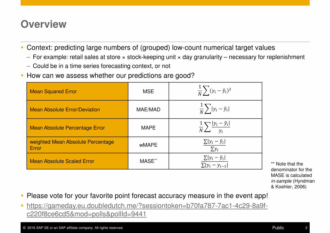
� Context: predicting large numbers of (grouped) low-count numerical target values

– For example: retail sales at store × stock-keeping unit × day granularity – necessary for replenishment

– Could be in a time series forecasting context, or not

� How can we assess whether our predictions are good?

� Please vote for your favorite point forecast accuracy measure in the event app!

� https://gameday.eu.doubledutch.me/?sessiontoken=b70fa787-7ac1-4c29-8a9f-c220f8ce6cd5&mod=polls&pollId=9441

Mean Squared Error MSE1� � �� − ��

Mean Absolute Error/Deviation MAE/MAD1� � �� − ��

Mean Absolute Percentage Error MAPE1� � �� − ��

��

weighted Mean Absolute Percentage Error

wMAPE∑ �� − ��

∑��

Mean Absolute Scaled Error MASE**∑ �� − ��

∑|�� − ��| ** Note that the denominator for the

MASE is calculated in-sample (Hyndman & Koehler, 2006)


Overview

� Context: predicting large numbers of grouped low-count numerical target values

– For example: retail sales at store × stock-keeping unit × day granularity – necessary for replenishment

– Could be in a time series forecasting context, or not

� How can we assess whether our predictions are good?

� However, optimizing (some of) these can lead to systematically biased predictions!

� Better: predict & assess full densities!

� (Full paper here: http://dx.doi.org/10.1016/j.ijforecast.2015.12.004)

“Robust”? Defined? Comparable*? Intuitive?

MSE1� � �� − ��

� ��

MAE1� � �� − ��

MAPE1� � �� − ��

�� ((�)) � ��

wMAPE∑ �� − ��

∑�� (�) � ��

MASE**∑ �� − ��

∑|�� − ��| �� (�) �

** Note that the denominator for the

MASE is calculated in-sample (Hyndman & Koehler, 2006)

* Comparability between

groups/series on different levels, e.g., fast vs. slow selling products

Part 1

Part 2


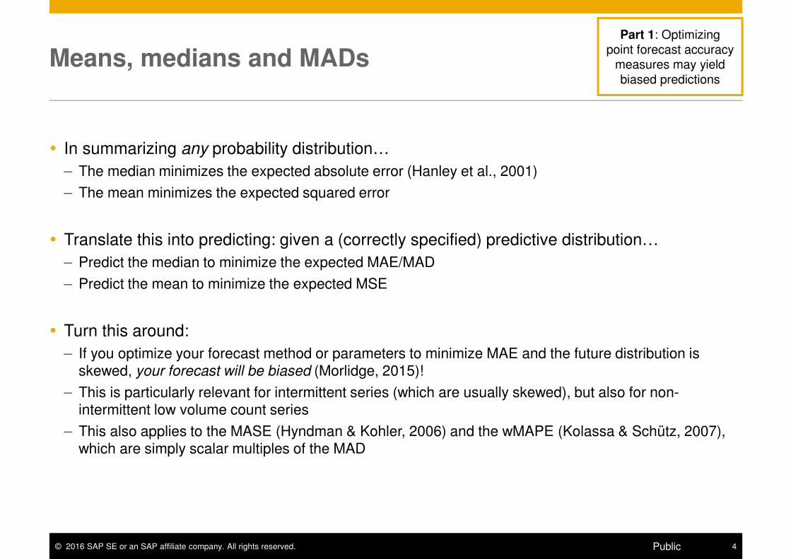
Means, medians and MADs

� In summarizing any probability distribution…

– The median minimizes the expected absolute error (Hanley et al., 2001)

– The mean minimizes the expected squared error

� Translate this into predicting: given a (correctly specified) predictive distribution…

– Predict the median to minimize the expected MAE/MAD

– Predict the mean to minimize the expected MSE

� Turn this around:

– If you optimize your forecast method or parameters to minimize MAE and the future distribution is skewed, your forecast will be biased (Morlidge, 2015)!

– This is particularly relevant for intermittent series (which are usually skewed), but also for non-intermittent low volume count series

– This also applies to the MASE (Hyndman & Kohler, 2006) and the wMAPE (Kolassa & Schütz, 2007), which are simply scalar multiples of the MAD

Part 1: Optimizing

point forecast accuracy measures may yield

biased predictions


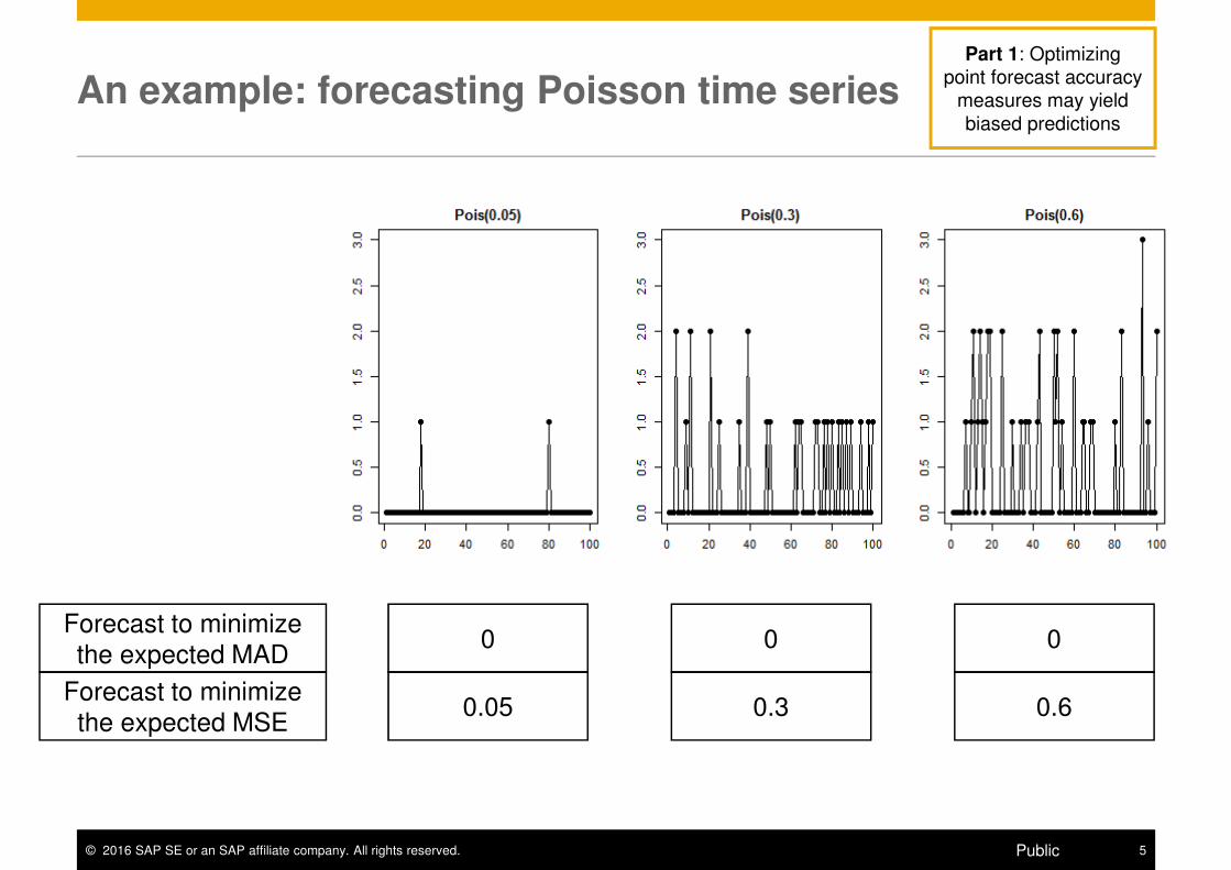
An example: forecasting Poisson time series

000

0.60.30.05

Forecast to minimize the expected MAD

Forecast to minimize the expected MSE

Part 1: Optimizing

point forecast accuracy measures may yield

biased predictions


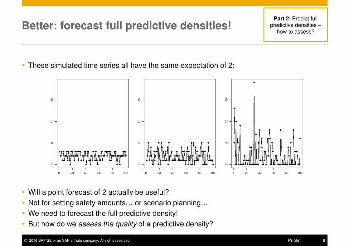
Better: forecast full predictive densities!

� These simulated time series all have the same expectation of 2:

� Will a point forecast of 2 actually be useful?

� Not for setting safety amounts… or scenario planning…

� We need to forecast the full predictive density!

� But how do we assess the quality of a predictive density?

Part 2: Predict full

predictive densities –

how to assess?


The Probability Integral Transformation (PIT)

� Assume predictive distributions with densities �� and cumulative distribution functions �� Transform observations ��:

�� ≔ �� ≤ �� = �� = � ��

�� If the predictive distributions are correct, �� = � and �� = ��, then �� ∼ �(0,1) – this can be

tested (e.g., Ledwina, 1994; Berkowitz, 2001; or others)



how to assess?


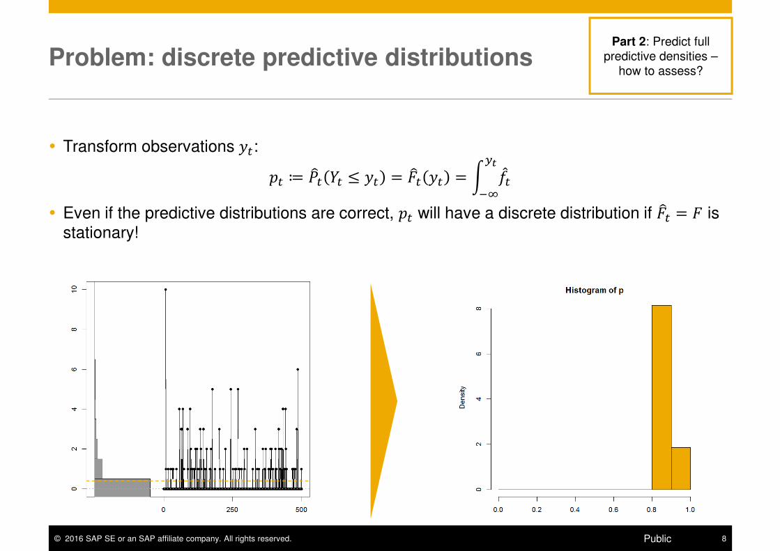
Problem: discrete predictive distributions

� Transform observations ��:�� ≔ �� ≤ �� = �� = � ��

��

�� Even if the predictive distributions are correct, �� will have a discrete distribution if �� = � is

stationary!



how to assess?


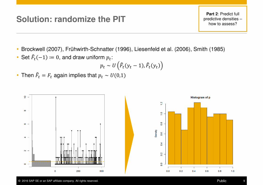
Solution: randomize the PIT

� Brockwell (2007), Frühwirth-Schnatter (1996), Liesenfeld et al. (2006), Smith (1985)

� Set �� −1 ≔ 0, and draw uniform ��:�� ∼ � �� − 1 , ��

� Then �� = �� again implies that �� ∼ �(0,1)



how to assess?


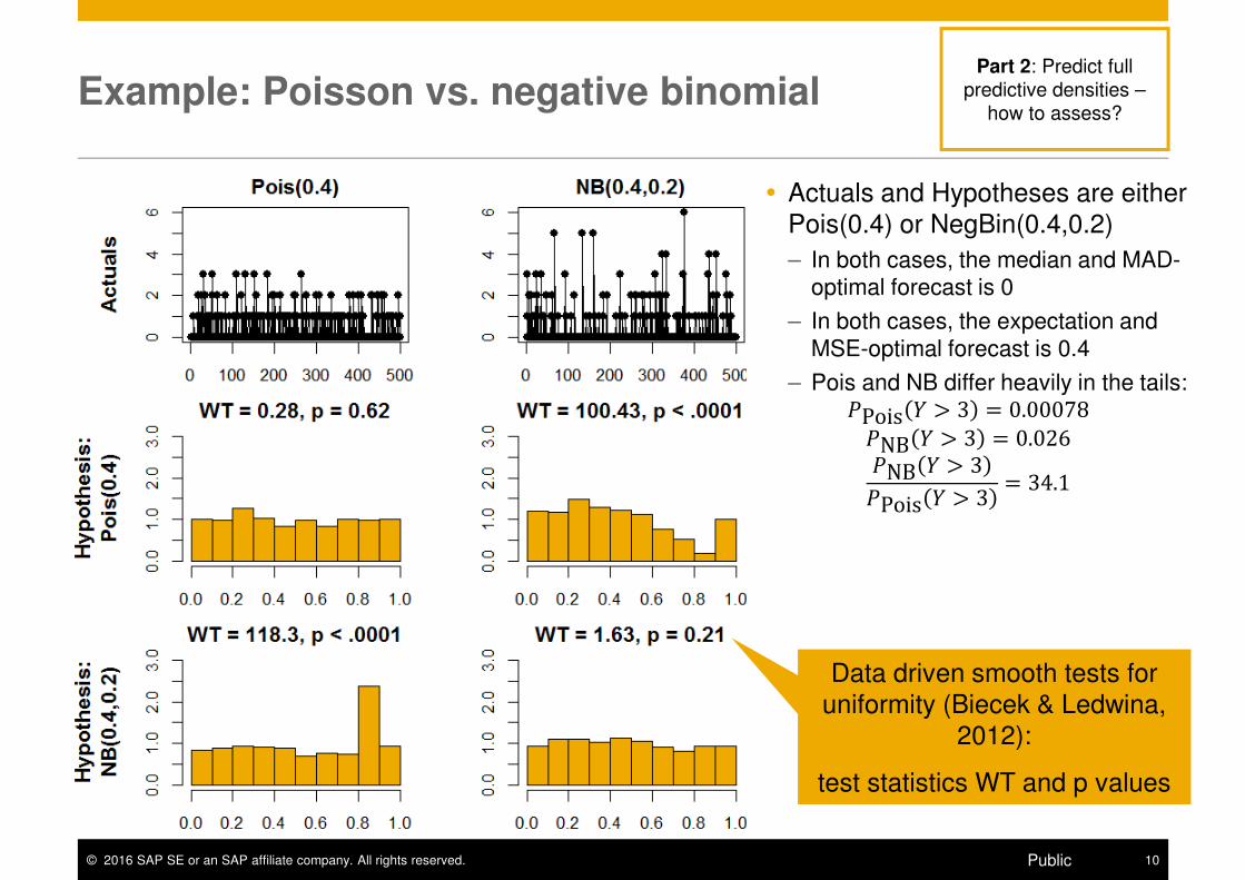
Example: Poisson vs. negative binomial

Data driven smooth tests for uniformity (Biecek & Ledwina,

2012):

test statistics WT and p values

� Actuals and Hypotheses are either Pois(0.4) or NegBin(0.4,0.2)

– In both cases, the median and MAD-optimal forecast is 0

– In both cases, the expectation and

MSE-optimal forecast is 0.4

– Pois and NB differ heavily in the tails:�Pois � > 3 = 0.00078

�NB � > 3 = 0.026�NB � > 3

�Pois � > 3 = 34.1



how to assess?


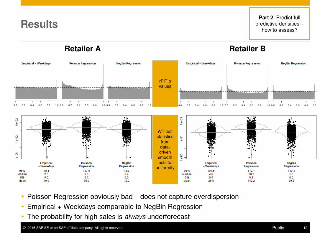
How to apply this to grouped data,

e.g. multiple time series?

� Two possible summaries:

– Simply “stack” all p values and test this big vector for uniformity

– Test each series’ p values for uniformity, yielding a test statistic WT for each series – plot, summarize, compare these

� Illustration: two datasets with daily sales from European retailers

– 1000 series each

– Forecast horizon up to 100 days for each series

� Try multiple forecasting approaches – here, look at three:

– Empirical + Weekday

o Density forecast for next Friday is just the historically observed distribution of Friday sales

– Poisson Regression

– NegBin Regression

o Regressions include day of week, price, trend and Christmas



how to assess?


Results

Retailer A Retailer B

� Poisson Regression obviously bad – does not capture overdispersion

� Empirical + Weekdays comparable to NegBin Regression

� The probability for high sales is always underforecast



how to assess?

rPIT p values

WT test statistics

from data-driven

smooth tests for

uniformity


Conclusion

� Do not rely on the MAE et al. to find an unbiased point forecast

– If you do need to report MAE/MAPE/wMAPE/MASE, also report bias

– For point predictions, use MSE, or RMSE, or a scaled RMSE that is comparable between scales

� Better: forecast and assess full predictive densities, as we did here

– Alternative to the rPIT: proper scoring rules (see the paper)

– Possibly assess misspecified dynamics/correlations

o E.g., AR(7) error structure by comparing against Markov Chain alternatives

o This is hard for low counts (low power!)

� Finally: assess the consequences of your forecast

– “Cost of Forecast Error”

– “Forecast Value Added”

– These will usually include both interval forecasts/predictive distributions and subsequent processes, like logistical optimization for replenishment


References

� Berkowitz, J. (2001). Testing Density Forecasts, With Applications to Risk Management. Journal of Business and

Economic Statistics, 19, 465-474

� Biecek, P. & Ledwina, T. (2012). ddst: Data driven smooth test. R package version 1.03. http://CRAN.R-

project.org/package=ddst

� Brockwell, A. E. (2007). Universal residuals: A multivariate transformation. Statistics & Probability Letters, 77,

1473–1478.

� Frühwirth-Schnatter, S. (1996). Recursive residuals and model diagnostics for normal and non-normal state

space models. Environmental and Ecological Statistics, 3, 291–309.

� Hanley, J. A.; Joseph, L.; Platt, R. W.; Chung, M. K. & Belisle, P. (2001). Visualizing the Median as the Minimum-

Deviation Location. The American Statistician, 55, 150-152

� Hyndman, R. J. & Koehler, A. B. (2006). Another look at measures of forecast accuracy. International Journal of

Forecasting, 22, 679-688

� Kolassa, S. & Schütz, W. (2007). Advantages of the MAD/Mean ratio over the MAPE. Foresight, 6, 40-43

� Liesenfeld, R., Nolte, I., & Pohlmeier, W. (2006). Modelling financial transaction price movements: a dynamic

integer count data model. Empirical Economics, 30, 795–825

� Ledwina, T. (1994). Data-Driven Version of Neyman's Smooth Test of Fit. Journal of the American Statistical

Association, 89, 1000-1005

� Morlidge, S. (2015). Measuring the Quality of Intermittent Demand Forecasts: It’s Worse than We’ve Thought!

Foresight, 37, 37-42

� Smith, J. Q. (1985). Diagnostic checks of non-standard time series models. Journal of Forecasting, 4, 283–291

© 2014 SAP SE or an SAP affiliate company. All rights reserved.

Thank you!

Contact information:

Stephan Kolassa

[email protected] ExpertProducts & Innovation Suite Engineering Consumer IndustriesSAP Switzerland


© 2016 SAP SE or an SAP affiliate company.

All rights reserved.

No part of this publication may be reproduced or transmitted in any form or for any purpose without the express permission of SAP SE or an SAP affiliate company.

SAP and other SAP products and services mentioned herein as well as their respective logos are trademarks or registered trademarks of SAP SE (or an SAP affiliate company) in Germany and other countries. Please see http://global12.sap.com/corporate-en/legal/copyright/index.epx for additional trademark information and notices.

Some software products marketed by SAP SE and its distributors contain proprietary software components of other software vendors.

National product specifications may vary.

These materials are provided by SAP SE or an SAP affiliate company for informational purposes only, without representation or warranty of any kind, and SAP SE or its affiliated companies shall not be liable for errors or omissions with respect to the materials. The only warranties for SAP SE or SAP affiliate company products and services are those that are set forth in the express warranty statements accompanying such products and

services, if any. Nothing herein should be construed as constituting an additional warranty.

In particular, SAP SE or its affiliated companies have no obligation to pursue any course of business outlined in this document or any related presentation, or to develop or release any functionality mentioned therein. This document, or any related presentation, and SAP SE’s or its affiliated companies’ strategy and possible future developments, products, and/or platform directions and functionality are all subject to change and may be changed by SAP SE or its affiliated companies at any time for any reason without notice. The information in this document is not a commitment,

promise, or legal obligation to deliver any material, code, or functionality. All forward-looking statements are subject to various risks and uncertainties that could cause actual results to differ materially from expectations. Readers are cautioned not to place undue reliance on these forward-looking statements, which speak only as of their dates, and they should not be relied upon in making purchasing decisions.

assessing predictive count data distributions · assessing predictive count data distributions...

Documents