assessing positive matrix factorization model ﬁt: a new

Atmos. Chem. Phys., 9, 497–513, 2009www.atmos-chem-phys.net/9/497/2009/© Author(s) 2009. This work is distributed underthe Creative Commons Attribution 3.0 License.

AtmosphericChemistry

and Physics

Assessing positive matrix factorization model fit: a new method toestimate uncertainty and bias in factor contributions at themeasurement time scale

J. G. Hemann1, G. L. Brinkman 2, S. J. Dutton2, M. P. Hannigan2, J. B. Milford 2, and S. L. Miller 2

1Department of Applied Mathematics, University of Colorado, Boulder, USA2Department of Mechanical Engineering, University of Colorado, Boulder, USA

Received: 3 January 2008 – Published in Atmos. Chem. Phys. Discuss.: 14 February 2008Revised: 4 December 2008 – Accepted: 5 December 2008 – Published: 22 January 2009

Abstract. A Positive Matrix Factorization receptor modelfor aerosol pollution source apportionment was fit to a syn-thetic dataset simulating one year of daily measurements ofambient PM2.5 concentrations, comprised of 39 chemicalspecies from nine pollutant sources. A novel method wasdeveloped to estimate model fit uncertainty and bias at thedaily time scale, as related to factor contributions. A circularblock bootstrap is used to create replicate datasets, with thesame receptor model then fit to the data. Neural networks aretrained to classify factors based upon chemical profiles, asopposed to correlating contribution time series, and this clas-sification is used to align factor orderings across the modelresults associated with the replicate datasets. Factor contri-bution uncertainty is assessed from the distribution of resultsassociated with each factor. Comparing modeled factors withinput factors used to create the synthetic data assesses bias.The results indicate that variability in factor contribution es-timates does not necessarily encompass model error: contri-bution estimates can have small associated variability acrossresults yet also be very biased. These findings are likely de-pendent on characteristics of the data.

1 Introduction

Air pollution comprised of particulate matter smaller than2.5µm in aerodynamic diameter (PM2.5) has been associatedwith a significant increased risk of morbidity and mortality(Dockery et al., 1993; Pope et al., 2002; Peel et al., 2005).Existing regulations have focused on average and peak PM2.5concentrations (µg m−3). To help policy makers design more

Correspondence to:J. G. Hemann([email protected])

targeted and cost-effective approaches to protecting publichealth and welfare, an understanding of the association be-tween PM2.5 sources and morbidity and/or mortality needsto be developed.

The Denver Aerosol Sources & Health study (DASH) hasbeen undertaken to understand the sources of PM2.5 that aredetrimental to human health. PM2.5 filter samples are col-lected daily from a centrally located site in Denver, CO. Spe-ciated PM2.5 is quantified including sulfate, nitrate, bulk el-emental and organic carbon, trace metals, and trace organiccompounds. These speciated PM2.5 data are used as input toa receptor model, Positive Matrix Factorization (PMF), forpollution source apportionment. The PMF model fit yieldscharacterizations of pollution sources, known asfactors, withrespect to their contributions to total measured PM2.5, as wellas their chemical profiles. Ultimately, an association willbe explored between the individual factor contributions andshort-term, adverse health effects, including daily mortality,daily hospitalizations for cardiovascular and respiratory con-ditions, and measures of poor asthma. For example, histori-cal records of daily hospitalizations due to respiratory prob-lems might be regressed against the daily concentrations ofPM2.5 pollution from diesel fuel combustion (as estimatedby PMF) over the same time span. Having measures of un-certainty associated with the contribution of diesel fuel com-bustion to PM2.5, at the daily time scale, may lead to morereliable characterization of the role diesel fuel combustionhas in daily health effects data.

PMF is a factor analytic method developed by Paatero andTapper in 1994 (Paatero and Tapper, 1994) that has beenwidely used for pollution source apportionment modeling(Anderson et al., 2001; Kim and Hopke, 2007; Larsen andBaker, 2003; Lee et al., 1999; Polissar et al., 1998; Ramadanet al., 2000). The objective of this paper is to present a novel

Published by Copernicus Publications on behalf of the European Geosciences Union.

http://creativecommons.org/licenses/by/3.0/

498 J. G. Hemann et al.: A new method to estimate PMF model uncertainty

method that has been developed to quantify uncertainty andbias in a PMF source apportionment model as it is applied tospeciated PM2.5 data. Uncertainty in a PMF solution existsat a number of levels and is important to quantify, especiallyif the solutions will inform environmental and health policydecisions.

Uncertainty can stem from the data and from the PMFmodel itself. With respect to the data, uncertainty in the so-lution is imparted through measurement error as well as ran-dom sampling error. For the PMF model, there is generally“rotational ambiguity” in the solutions (i.e. solutions are notunique); further, solutions based upon the same data can varydepending upon how the model parameters are set. Past stud-ies have considered these aspects, primarily by using the sta-tistical method of the bootstrap to analyze model fit results.For example, Heidam (1987) considered the uncertainty infactor profiles due to receptor model uncertainty by varyingthe model parameters in models fit to bootstrapped datasets.

The Environmental Protection Agency’s Office of Re-search and Development distributes two software products,EPA PMF 1.1 (Eberly, 2005) and EPA Unmix 6.0 (Norriset al., 2007), which incorporate the bootstrap to analyze re-ceptor model fit results. The software can be used to assessuncertainty in factor profile estimates and has been used bystudies such as Chen et al. (2007) and Olson et al. (2007) tocharacterize sources of PM2.5. Few studies, however, haveaddressed uncertainty in factor contribution estimates. Twoexamples are Nitta et al. (1994) and Lewis et al. (2003),though the estimates come from different source apportion-ment models and pertain to average contribution variability.

The method presented in this paper estimates, at the mea-surement time scale, bias and variability due to randomsampling error in factor contribution estimates. Replicatedatasets are created using a circular block bootstrap, andthe subsequent application of two novel techniques makesuch estimation possible. First, neural networks are used formatching factors across PMF results on that data. Secondthe measurements resampled across the replicate datasets aretracked within the PMF solutions. This discussion describesthe method in the context of application to a synthetic PM2.5dataset, which was designed to simulate DASH data, fit bythe PMF model. Using synthetic data allows assessment ofmodel fit as well as a way to validate the method itself.

2 Methodology

Presented here is a method of assessing uncertainty in sourceapportionment model results using two different measures:bias and variability due to random sampling error. Themethod goes beyond computing these measures in terms of“average values” and gives estimates at the measurementtime scale.

A synthetic time series of daily PM2.5 measurements isused in which the concentrations of chemical species are de-

rived from published source profiles and source contributionsconsistent with the Denver area. The solution from applyingPMF can be compared with “known” profiles and contribu-tions, allowing estimates of bias to be computed.

A circular block bootstrap generates additional data by re-sampling, with replacement, from the original synthetic mea-surement series. Each new dataset, or replicate, is again fitby the PMF model to apportion the PM2.5 mass to factors.

The first novel aspect pertains to how factors are sortedbetween solutions. For each solution the factors should cor-respond to the same real-world pollution sources. The fac-tors need to be aligned such that “factork” in each solutionalways refers to the same factor. To accomplish this factoralignment, or matching, the standard approach has been touse scalar metrics like linear correlation to match a factorfrom one solution to the “closest” factor in another solution.This is the approach taken by the EPA PMF 1.1 software,where it is specifically the time series of factor contributionsthat are matched between solutions. In contrast, the presentwork takes the novel approach of using Multilayer FeedForward Neural Networks (NN), trained to perform patternrecognition, to align factors between PMF solutions. Further,using the intuitive notion that pollution sources are character-ized best by the chemical species they emit, the matching isbased on factors’ profiles rather than their contribution timeseries. The NN approach is a robust factor matching tech-nique: it avoids the sensitivity to outliers that is problematicwhen using measures such as linear correlation and replacesit with a method that is capable of capturing linear as well asnon-linear relationships.

The second novel aspect in the method presented hereis the tracking of the measurement days resampled in eachbootstrapped dataset. Through this bookkeeping it is possi-ble to arrive at a collection of PMF results for each factor’scontribution on each day. Accordingly, descriptive statisticscan be computed for each factor contribution on each day.

2.1 Positive Matrix Factorization

PM2.5 pollution is typically comprised of dozens of chemicalspecie emitted from multiple sources. The concentration ofeach species may be treated as a random variable observedover time. The statistical technique offactor analysiscan beused to explain the variability in these observations as linearcombinations of some unknown subset of the sources, calledfactors. In traditional factor analysis approaches, includingPrincipal Components Analysis, the variance-covariance ma-trix of the observations is used in an eigen-analysis to find thefactors that explain most of the variability observed. The un-certainty in the observations, for all variables, is assumed tobe independent and normally distributed. These assumptionsare often not valid in the context of air pollution measure-ment data. In contrast, PMF – a receptor-based source appor-tionment model – offers an alternative technique that is basedupon a least squares method, and measurement uncertainties

Atmos. Chem. Phys., 9, 497–513, 2009 www.atmos-chem-phys.net/9/497/2009/

J. G. Hemann et al.: A new method to estimate PMF model uncertainty 499

can be specific to each observation, correlated, and non-normal in distribution. Further, the factors resultant fromPMF need not be orthogonal, which is an important qualitywhen trying to associate modeled factors to real-world pollu-tion sources that can be highly temporally correlated but arenonetheless important to characterize separately (e.g. dieselversus gasoline fuel combustion).

Given a matrix of observed PM2.5 concentrations,X, PMFattempts to solve

X = GF + E (1)

by finding the matricesG andF that recoverX most closely,with all elements ofG andF strictly non-negative.G is thematrix of factor contributions (or “scores” in traditional fac-tor analysis terminology), whereGik is the concentration fac-tor k contributed to the total PM2.5 observed in samplei. Fis the matrix of factor profiles (or “loadings”), whereFkj isthe fraction at which speciesj makes up factork. Finally, Eis the matrix of residuals defined by

Eij = Xij −

p∑k=1

GikFkj (2)

G andF are found through an alternating least squares al-gorithm that minimizes the sum of the normalized, squaredresiduals,Q

Q =

n∑i=1

m∑j=1

(Eij

Sij

)2

(3)

whereEij is weighted bySij , the uncertainty associated withthe measurement of thej th pollutant species in thei sample.The ability to weight specific observations with specific un-certainties allows PMF to handle data that include heteroge-nous measurement uncertainty, outliers, values below mea-surement detection limits, and missing values. As such, PMFcan often yield better results than traditional factor analysismethods (Huang et al., 1999).

An algorithm for implementing PMF is available as a com-mercial software library, PMF2 (Paatero, 1997). The workpresented here uses PMF2 version 4.2, and specifically, thepmf2wopt executable file (Paatero, 2007). PMF2 has numer-ous optimization parameters that can be set by the user, andmethods of choosing these values have been published else-where (Paatero, 2000; Paatero et al., 2002, 2005). Since thefocus of this paper is on a method of assessing uncertaintyand bias in PMF solutions, the discussion of fine-tuning thenumerous algorithm parameters is kept to a minimum. TwoPMF2 parameters are especially important to the PMF modelfit and deserve mention. First, the number of factors in themodel,p, must be set by the user. In the present work, eightand nine factor solutions are considered, with the primaryfocus on the results for the nine factor solutions. The otherimportant parameter is FPEAK, which controls the rotationalfreedom of the possible solutions. It is advised that FPEAK

values range between−1 and 1, with positive values causingextremes in theF matrix (values near 0 or 1) and negative val-ues causing extremes in theG matrix. In the present work,FPEAK is zero for all PMF2 solutions, which corresponds tothe default setting.

2.2 Synthetic data

Given that the results of pollution source apportionmentmodels may ultimately be used as critical components of en-vironmental policy and regulatory decisions, it is especiallyimportant to assess their quality. One approach for evaluatingreceptor models is the use of synthetic data, which is definedas simulated PM2.5 measurements rather than actual obser-vations (Willis, 2000). Predefined sources are used, alongwith their respective contributions and profiles, to create theG andF matrices in Eq. (2). WithG andF definedX can becalculated directly and given as input (along with uncertaintyestimates) to the PMF2 software, where the resultantG andF matrices can then be compared with the actual values toassess model fit.

The method of creating synthetic datasets followed in thispaper is described in detail in Brinkman et al. (2006) andVedal et al. (2007). Briefly, nine pollutant sources were used(Table 1), which contributed concentrations of 39 chemicalspecies (Table 3), over 365 synthetic sampling days. Thesynthetic measurements were assumed to come from a singlereceptor site. Table 1 also lists the references used to generatethe annual contributions, chemical profile, temporal patternsand variability for each source. Table 2 shows the lag zerocross correlations between the source contributions. With re-spect to PMF modeling, the relatively high cross-correlationsbetween some of the input source contribution time series hasthe implication that some of these sources may be harder tocleanly separate from others.

Distinct time series for the contributions from each sourcewere generated by starting with average contribution es-timates from preliminary DASH studies and the NorthernFront Range Air Quality Study (Watson et al., 1998), thenadding day-to-day variations reflecting both random variabil-ity and hypothesized weekly or seasonal patterns, as appro-priate. Daily totals for the nine source contributions werenormalized to match actual daily PM2.5 levels observed inDenver in 2003. It should be noted that the presence of ad-ditional sources, such as secondary organic aerosols, couldcomplicate application of PMF to observed data. The ma-trix of data uncertainties,S from Eq. (3), is computed asfollows. Measurement detection limits, detection limit un-certainty, and measurement uncertainty associated with typ-ical analytical techniques used to speciate PM2.5 filter sam-ples (Ion Chromatography, Thermal Optical Transmission,and Gas Chromatography/Mass Spectrometry), were incor-porated into the PMF input via

Sij =

√(αjXij

)2+

(βjDj

)2 (4)

www.atmos-chem-phys.net/9/497/2009/ Atmos. Chem. Phys., 9, 497–513, 2009


Table 1. Synthetic PM2.5 sources.

Source References

Secondary Ammonium Sulfate Lough (2004)Secondary Ammonium Nitrate Lough (2004)Gasoline Vehicles Watson et al. (1998); Chinkin et al. (2003);

Cadle et al. (1999); Hildeman et al. (1991); Rogge et al. (1993a)Diesel Vehicles Watson et al. (1998); Chinkin et al. (2003);

Hildeman et al. (1991); Rogge et al. (1993a); Schauer (1998)Paved Road Dust Watson et al. (1998); Chinkin et al. (2003); Hildeman et al. (1991);

Rogge et al. (1993b)Wood Combustion Watson et al. (1998); Fine et al. (2004)Meat Cooking Watson et al. (1998); Schauer et al. (1999)Natural Gas Combustion Hildeman et al. (1991); Hannigan (1997); Rogge et al. (1993d)Vegetative Detritus Hildeman et al. (1991); Hannigan (1997); Rogge et al. (1993c)

Table 2. Source contribution cross-correlations, Lag=0.

Amm Sulfate Amm Nitrate Gasoline Diesel Road Dust Wood Meat Natural Gas Veg

Ammonium Sulfate 1 0.55 0.89 0.57 0.73 0.24 0.81 0.68 0.49Ammonium Nitrate . 1 0.39 0.26 0.32 0.82 0.35 0.8−0.15Gasoline Vehicles . . 1 0.62 0.74 0.13 0.81 0.64 0.54Diesel Vehicles . . . 1 0.61 0.08 0.28 0.33 0.31Paved Road Dust . . . . 1 0.13 0.57 0.5 0.37Wood Combustion . . . . . 1 0.14 0.77−0.34Meat Cooking . . . . . . 1 0.64 0.53Natural Gas . . . . . . . 1 0.08Vegetative Detritus . . . . . . . . 1

where for speciesj , αj is the measurement uncertainty,βj isthe detection limit uncertainty, andDj is the detection limit.Table 3 contains theα, β andD associated with each species.The Sij uncertainties were incorporated into the final datamatrixX′ with the following formula

X′

ij = Xij + SijZij (5)

whereZij is a random number drawn from a standard normaldistribution. If X′

ij was less than the detection limit associ-ated with measuring speciesj , then a value of one-half thedetection limit was substituted in the final data matrix.

2.3 The bootstrap

The bootstrap is a computationally intensive method for es-timating the distribution of a statistic, the statistic itself be-ing an estimator of some parameter of interest (Efron, 1979).The essence of the method is to create replicate data by re-sampling, with replacement, from the original observationsof a random variable. For each replicate dataset the statisticof interest is computed, and the distribution of these valuesserves as an estimate for the random sampling distribution

of the statistic. The properties of this distribution are thenused to make inferences about the parameter of interest. Inthe present context, each pollutant species’ time series repre-sents realizations of a random variable. TheF andG matri-ces resulting from PMF’s fitting of these data are functionsof these random variables, thus, each element of those ma-trices may be considered a statistic. Previous studies usingPMF have focused on analyzing theF matrix, the matrix offactor profiles. This discussion takes a different tack, withthe statistic of interest being each element of theG matrix,the matrix of factor contributions over time.

2.3.1 Dependent data considerations

Much of bootstrap theory is based upon the assumption thatthe data are comprised of observations of independent andidentically distributed (iid) random variables. Time seriesdata, however, are typically serially correlated. Singh (1981)showed that the bootstrap can be inconsistent in estimat-ing the distribution of statistics based upon dependent data.Since then, numerous modifications of the original iid boot-strap have been formulated to better handle dependent data



Table 3. Synthetic PM2.5 species, measurement detection limits(D), measurement errors (α), and detection limit uncertainties (β).

Species # Species Name D α β

(ng/m3) (%) (%)1 Elemental Carbon 13 10 1972 Organic carbon 3.6 14 1003 Nitrate 0.094 5 2964 Sulfate 0.20 3 6145 Ammonium 0.22 6 10576 n-Tricosane 0.97 8 1257 n-Tetracosane 1.4 9 1868 n-Pentacosane 1.1 8 2099 n-Hexacosane 1.1 7 21410 n-Heptacosane 1.1 6 24511 n-Octacosane 1.2 4 20712 n-Nonacosane 0.96 4 23413 n-Triacontane 0.92 6 18514 n-Hentriacontane 0.92 8 14515 n-Dotriacontane 0.23 9 10816 n-Tritriacontane 0.16 9 9617 n-Tetratriacontane 0.093 8 9318 Oleic acid 6.6 14 3919 n-Pentadecanoic acid 1.4 15 23520 n-Hexadecanoic acid 48 16 11621 n-Octadecanoic acid 26 14 13722 Acetovanillone 0.064 14 21223 Coniferyl aldehyde 1.9 14 8624 Syringaldehyde 0.62 12 13925 Acetosyringone 0.97 11 46826 Retene 0.079 12 31627 Alkyl Cyclohexanes 0.085 8 12328 Benzo[k]fluoranthene 0.0068 10 64929 Benzo[b]fluoranthene 0.0068 10 64930 Benzo[e]pyrene 0.0056 15 27231 Indeno[1,2,3-cd]pyrene 0.017 13 105232 Indeno[1,2,3-cd]fluoranthene 0.021 13 105233 Benzo[ghi]perylene 0.023 10 16934 Coronene 0.021 13 2335 Cholestanes 0.21 8 6536 Hopane 0.045 17 20237 Norhopane 0.050 19 11338 Homohopanes 0.013 18 34239 Oxygen 41 3 106

(Carlstein, 1986; Kunsch, 1989; Liu and Singh, 1992). Oneapproach often used for time series data is to resample blocksof successive observations. If the blocks are of sufficientlength, l, and the series is only weakly dependent, then theobservations within each block may be considered indepen-dent of the observations within the other blocks. Further, ifthe series is stationary then all blocks will share the samel-dimensional joint distribution. These two conditions allowthe blocks themselves to be treated as independent and iden-tically distributed observations to which the iid bootstrap canbe applied. This approach is currently used by the EPA PMF1.1 software tool, which uses a 3-day, Moving Block Boot-strap (MBB).

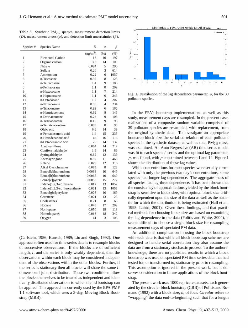
Fig. 1. Distribution of the lag dependence parameter,p, for the 39pollutant species.

In the EPA’s bootstrap implementation, as well as thisstudy, measurement days are resampled. In the present case,realizations of a composite random variable comprised of39 pollutant species are resampled, with replacement, fromthe original synthetic data. To investigate an appropriatebootstrap block size the serial correlation of each pollutantspecies in the synthetic dataset, as well as total PM2.5 mass,was examined. An Auto Regressive (AR) time series modelwas fit to each species’ series and the optimal lag parameter,p, was found, withp constrained between 1 and 14. Figure 1shows the distribution of these lag values.

While concentrations for most species were serially corre-lated with only the previous two day’s concentrations, somespecies had longer lag-dependence. The aggregate mass ofall species had lag-three dependence. It has been shown thatthe consistency of approximations yielded by the block boot-strap is sensitive to block size, with optimal block size criti-cally dependent upon the size of the data as well as the statis-tic for which the distribution is being estimated (Hall et al.,1995; Lahiri, 2001). Given these findings, and that practi-cal methods for choosing block size are based on examiningthe lag-dependence in the data (Politis and White, 2004), itseems difficult to choose a single block size for resamplingmeasurement days of speciated PM data.

An additional complication in using the block bootstrapwith such data is that while all block bootstrap schemes aredesigned to handle serial correlation they also assume thedata are from a stationary stochastic process. To the authors’knowledge, there are no published results in which a blockbootstrap was used on speciated PM time series data that hadtested for, or transformed to, stationarity prior to resampling.This assumption is ignored in the present work, but it de-serves consideration in future applications of the block boot-strap.

The present work uses 1000 replicate datasets, each gener-ated by the circular block bootstrap (CBB) of Politis and Ro-mano (1992) with a block size,b, of four. Circular refers to“wrapping” the data end-to-beginning such that for a length



N series,XN+k=Xk. A block length of four was chosensince the lag-dependence for mass was three days, and themajority of species had lag-dependence of five or less days.As an example, to create a bootstrap replicate data matrixX∗,let Y be a copy of the original matrixX, and append the firstb-1 rows ofX to the bottom ofY. Divide the rows ofY intoN consecutive sizeb blocks. IfXi andYi denote theith rowof X andY, respectively, then the blocks would be

block 1 : Y1, Y2, Y3, Y4=X1, X2, X3, X4block 2 : Y2, Y3, Y4, Y5=X2, X3, X4, X5...

block N : YN , YN+1, YN+2, YN+3=XN , X1, X2, X3

ConstructX∗ by selectingN/b blocks randomly, with re-placement, fromY. Construct an associated replicate matrixof uncertainties,S∗, by selecting these same blocks fromS.Note that ifN/b is not an integer, round up and truncate asneeded. For example, in the present case withN=365 andb=4, 92 blocks would be chosen to createX∗. The last threeelements of the 92nd block would not be used, yielding a to-tal of 365 rows (measurement days) resampled fromX. Im-portantly, under CBB resampling each row ofX has the sameprobability of being resampled, which is not the case underMBB resampling (Lahiri, 2003).

2.3.2 Record keeping

In the following results an important component in imple-menting the bootstrap is the tracking of days resampled ineach replicate dataset. Since the essence of bootstrapping isresampling with replacement it is possible that for any givenreplicate dataset some synthetic measurement days are in-cluded multiple times and other days are not included at all.By keeping track of which days are resampled in which repli-cate dataset it is possible to assess factor contribution uncer-tainty and bias at the daily time scale.

2.4 Factor matching

The use of the bootstrap yields a collection of factor contri-bution matrices,Gk, k=1,. . . ,B, whereB is the number ofbootstrap replicate datasets. The collection of matrices maybe considered as a single, three-dimensional matrixG′, withelementsG

′kij , i=0,. . . ,N-1; j=0,. . . ,P-1; k=0,. . . ,B,whereN

is the number of samples andP is the number of factors (notethat theG matrix associated with the original data and “basecase” solution is also included inG′). While the nature of thefactors that the PMF2 algorithm finds should be stable acrossthe “bootstrap” solutions, the ordering of the factors withinthose solutions may be different. Before computing statisticson the elements ofG′, the dimension indexed byj must besorted, such that across theB+1 matrices factorj is alwaysassociated with the same real-world pollution source. Thetypical approach to matching and sorting factors has reliedon comparisons between the factor contribution time series,

using linear correlation to match a given factor from a boot-strap solution (or a factor from another analysis method) tothe “closest” factor in a base case solution.

There are several concerns with this approach. First,“closeness” is measured with a scalar metric that is highlysensitive to outliers. Second, the bootstrap replicate data setswill not preserve the temporal patterns seen in the originaldata when viewed over the course of the entire sampling pe-riod (although there are block bootstrap methods that seekto address this). Correlation ceases to be a useful measureonce there is no temporal consistency between the contribu-tion time series being compared. Third, there are no clearrules for what constitutes sufficient correlation, especially incases where two factors in one bootstrap solution are highly(or even poorly but equally) correlated with the same factorin the base case solution. The use of this metric invites “datadredging”, where the practitioner must make ad hoc choicesto separate and match factors.

The present discussion employs an approach that the au-thors believe to be novel and robust when applied to aerosolpollution data: neural networks are used to match factors be-tween bootstrap solutions and the base case solution basedupon their profiles. Matching on profiles addresses the sec-ond issue noted above, while the use of neural networksrather than correlation address the first and third issues. Theneed to classify a measured spectrum (profile) with a knownreference spectrum is a problem found in multiple scientificsettings, most notably in the analysis of stellar spectra anddata from hyperspectral remote sensing. Findings in thesefields may be useful in the modeling of aerosol pollution dataand are considered briefly. Work by van der Meer (2006)found that a spectral similarity measure based on correla-tion was more sensitive to noisy data than other traditionalmeasures based on Euclidean distance or spectral angle. Fur-ther, Shafri et al. (2007) reported that neural networks wereaccurate at classifying spectra from remote sensing of trop-ical forests, especially when compared to measures basedon spectral angle. Tong and Cheng (1999) found that us-ing neural networks was superior to using maximum corre-lation when classifying gas chromatography mass spectrom-etry data. Based on these findings, as well as the findingspresented herein, the authors are confident that using neuralnetworks to match factor profiles allows the bootstrap tech-nique to be better leveraged. The factor matching processcan be easily automated, adapted to complex patterns andnew, possibly noisy, data, and can avoid subjective “close-ness” thresholds required when using less robust measureslike correlation.



2.5 Neural networks

Artificial Neural Networks are statistical modeling methodscapable of characterizing highly non-linear functions, doingso by approximating the behavior of the brain. The term “ar-tificial” is used to distinguish this numerical approximationof biological, adaptive, cognition from those biological sys-tems. In general, this is understood in statistical modeling,and Artificial Neural Networks are simply referred to as Neu-ral Networks (NN). Excellent introductions to the subject canbe found in Haykin (1998) and Munakata (1998).

The specific type of NN used in this study is called aMulti-layer Feed Forward Network. This type of network relies onsupervised learning, in which the network is given inputs andlearns how to transform it into desired outputs. The learn-ing is encoded in numerical weights defining the strengthof connection between elements in the network. Weightsare found through quasi-Newton optimization incorporatedwith the backpropagation method, where “backpropagation”refers to the ground-breaking algorithm developed in the1970s and 1980s (Rumelhart et al., 1986; Werbos, 1974),allowing neural networks to classify linearly inseparable pat-terns. A trained network, characterized by its structure andits weights, can then be given novel input and transform it tothe correct output. In the present work that transformation isclassification: given a new factor profile, the trained neuralnetworks will classify it as a known type, or possibly classifyit as unknown.

2.5.1 Neural network configuration

In the present work, NN software from Visual Numerics’IMSL® C Numerical Library, version 6.0, is used. The struc-ture of the network is three fully connected layers, with 39nodes in the input layer, five nodes in the hidden layer, andtwo nodes in the output layer. All nodes in the hidden andoutput layers use a logistic activation function. The valuesof the two output nodes range between 0 and 1. An outputof [1,0] indicates a perfect match between an input factorprofile and the profile that particular network was trained toclassify as a “Yes”. Likewise, an output of [0,1] indicatesa perfect non-match between an input factor profile and thelearned profile. A “Yes” match is only possible if the firstoutput node has a value of at least 0.95, with the second nodehaving a value no larger than 0.05.

The performance of the network depends heavily upon thedata used for training. It is well established that neural net-works can be unstable when data used for training variesgreatly in scale; therefore, transformation and normalizationof data are typical preprocessing steps. In this study, factorprofiles are normalized before being learned by the networks.In “raw” form, the rows of theF matrix correspond to factorprofiles and each row sums to 1. Viewing factor profiles thisway can sometimes result in factors that are difficult to dis-tinguish, since some species will be present in large amounts

in many factors (e.g. organic carbon and oxygen). To makeplots of factor profiles more visibly distinguishable the fol-lowing normalization is done,

F′

kj =Fkj

P∑k=1

Fkj

(6)

whereF ′

kj is the relative weighting speciesj has in factork’s profile when considering all other factors. When viewingfactor profiles under this normalization, species common tomany factors are damped and marker species become morepronounced, as compared to viewing the raw profiles.

2.5.2 Training data

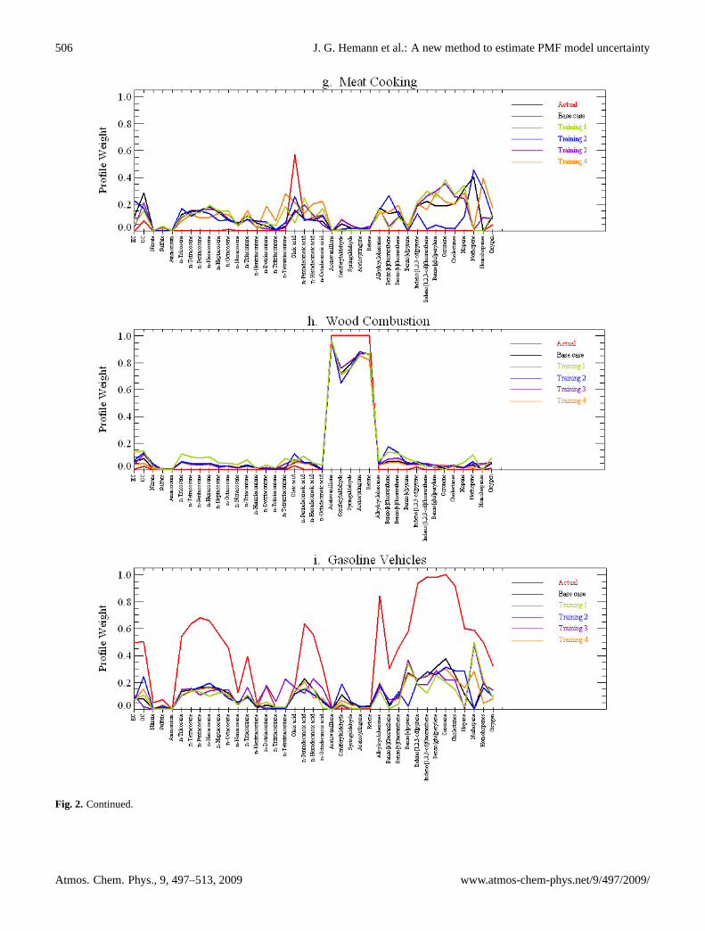
Five datasets were used to train the neural networks. Onedataset was the original synthetic data, with the remainingfour being bootstrap replicates. PMF was fit to each dataset,with the solution associated with the original dataset beingthe base case. The base case factor profiles were normal-ized (as described in Sect. 2.5.1), plotted, and visually com-pared to the normalized factor profile plots associated withthe bootstrap solutions. For each bootstrap solution the fac-tors were reordered to match the base case ordering. Figure 2shows the end result of this process, with the five factor pro-file plots used to classify each factor for the neural networktraining, as well as the actual profile used to create the origi-nal synthetic dataset.

2.6 Method steps

Having discussed the major components of the method foranalyzing factor contribution uncertainty and bias, it is help-ful to summarize their relationship in the following steps:

Step 1:Using the synthetic PM2.5 data and measurementuncertainties, compute a base case PMF model fit that hasP

factors. In the present work,P=9.Step 2: CreateT bootstrap replicate data matrices, with

corresponding uncertainty matrices, and fit each set withPMF. These results, in addition to the base case result, willserve as the neural network training data. In the present work,T =4.

Step 3:For each training replicate dataset, visually com-pare the normalized bootstrap factor profiles versus the nor-malized base case profiles, and define the factor matchingbetween the results. Reorder the factors to be consistent withthe base case factor ordering.

Step 4:For each factor, train a neural network to learn itsnormalized profile, as well as what is not its profile (thus,there will beP networks). For each factor there will beT +1profiles to be learned as “Yes” patterns. The remainingP -1profiles associated with the base case results are learned as“No” patterns.



Fig. 2. Plots of five normalized profiles for each factor learned by the neural networks. The thicker, black line represents the profile associatedwith the “base case” solution, while the thicker red line indicates the actual profile used to create the synthetic data. The remaining fourcolors correspond to factor profiles for “bootstrap” solutions based on resampled data. The factor ordering is now relative to the ordering inthe base case solution.



Fig. 2. Continued.



Step 5:CreateB new bootstrap replicate datasets and fiteach one with PMF. These results will be used to assess PMFmodel fit uncertainty. In the present work,B=1000

Step 6:For each bootstrap solution, allow each of theP

neural networks to examine each of theP normalized factorprofiles. Each network should identify a unique factor profileas a “Yes”, with all others classifying the profile as “No”.Reorder the factors in the bootstrap solution accordingly.

Step 7: Parse the factor contribution data by day-factorcombination. For example, consider examining the bias andvariability in the PMF solutions for the 3rd factor on day 126.All B+1 datasets would be searched for where the originalday 126 was resampled. This collection of indices wouldbe used to index into the 3rd column of the correspondingsolutions’G matrix to get factor 3’s contribution on day 126.The distribution of values is then compared with the actualcontribution used to create the original synthetic dataset.

Note that Step 3 is what establishes the supervisor for thesupervised learningalgorithm used to train the neural net-work. The role of the neural network is to learn the classifi-cation defined by an expert human observer, such that whennew factor profiles are analyzed, they are classified as wouldthe expert. In Step 6, it is possible that a bootstrap factorcan be matched with more than one base case factor, or, per-haps, it cannot be matched to any base case factor. In eithercase, that particular solution is excluded from the collectionof other solutions. In this way, after the last replicate datasethas been fit by PMF, the collection of solutions correspondto the case where bootstrap factors were matched uniquely tobase case factors.

3 Results

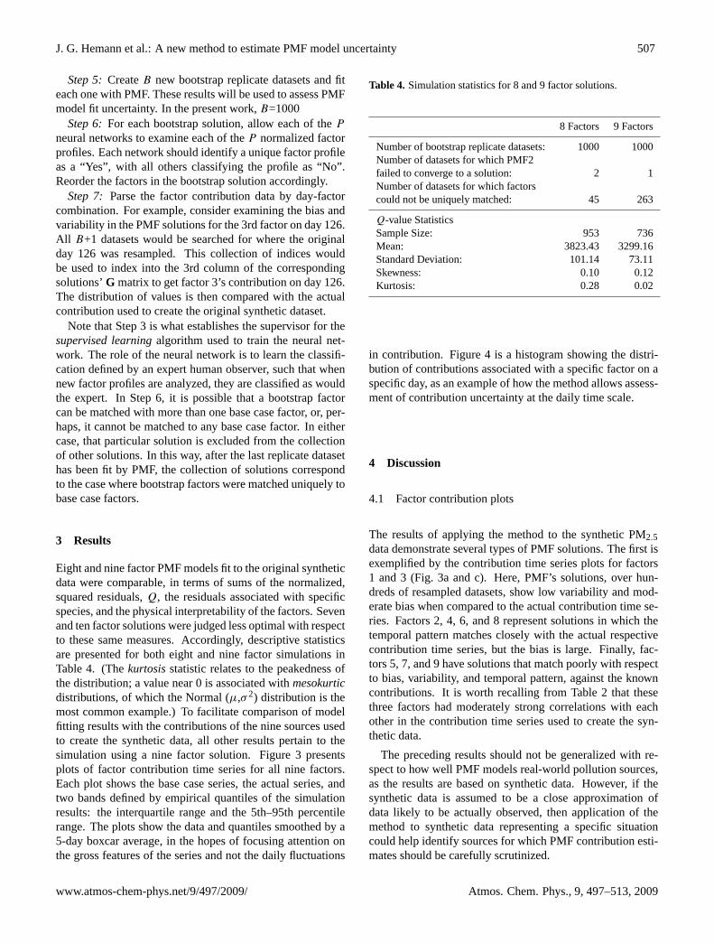
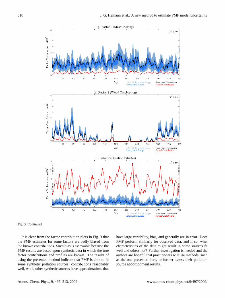
Eight and nine factor PMF models fit to the original syntheticdata were comparable, in terms of sums of the normalized,squared residuals,Q, the residuals associated with specificspecies, and the physical interpretability of the factors. Sevenand ten factor solutions were judged less optimal with respectto these same measures. Accordingly, descriptive statisticsare presented for both eight and nine factor simulations inTable 4. (Thekurtosisstatistic relates to the peakedness ofthe distribution; a value near 0 is associated withmesokurticdistributions, of which the Normal (µ,σ 2) distribution is themost common example.) To facilitate comparison of modelfitting results with the contributions of the nine sources usedto create the synthetic data, all other results pertain to thesimulation using a nine factor solution. Figure 3 presentsplots of factor contribution time series for all nine factors.Each plot shows the base case series, the actual series, andtwo bands defined by empirical quantiles of the simulationresults: the interquartile range and the 5th–95th percentilerange. The plots show the data and quantiles smoothed by a5-day boxcar average, in the hopes of focusing attention onthe gross features of the series and not the daily fluctuations

Table 4. Simulation statistics for 8 and 9 factor solutions.

8 Factors 9 Factors

Number of bootstrap replicate datasets: 1000 1000Number of datasets for which PMF2failed to converge to a solution: 2 1Number of datasets for which factorscould not be uniquely matched: 45 263

Q-value StatisticsSample Size: 953 736Mean: 3823.43 3299.16Standard Deviation: 101.14 73.11Skewness: 0.10 0.12Kurtosis: 0.28 0.02

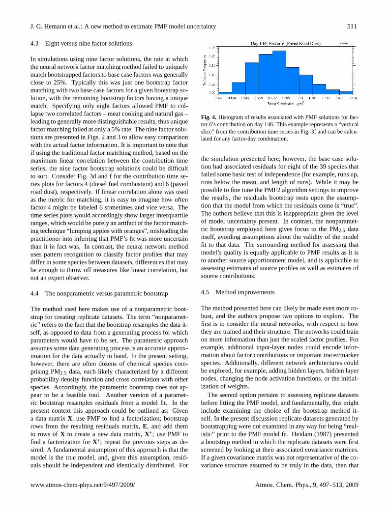
in contribution. Figure 4 is a histogram showing the distri-bution of contributions associated with a specific factor on aspecific day, as an example of how the method allows assess-ment of contribution uncertainty at the daily time scale.

4 Discussion

4.1 Factor contribution plots

The results of applying the method to the synthetic PM2.5data demonstrate several types of PMF solutions. The first isexemplified by the contribution time series plots for factors1 and 3 (Fig. 3a and c). Here, PMF’s solutions, over hun-dreds of resampled datasets, show low variability and mod-erate bias when compared to the actual contribution time se-ries. Factors 2, 4, 6, and 8 represent solutions in which thetemporal pattern matches closely with the actual respectivecontribution time series, but the bias is large. Finally, fac-tors 5, 7, and 9 have solutions that match poorly with respectto bias, variability, and temporal pattern, against the knowncontributions. It is worth recalling from Table 2 that thesethree factors had moderately strong correlations with eachother in the contribution time series used to create the syn-thetic data.

The preceding results should not be generalized with re-spect to how well PMF models real-world pollution sources,as the results are based on synthetic data. However, if thesynthetic data is assumed to be a close approximation ofdata likely to be actually observed, then application of themethod to synthetic data representing a specific situationcould help identify sources for which PMF contribution esti-mates should be carefully scrutinized.



Fig. 3. Comparison of PMF bootstrap solutions for factor contributions versus actual factor contributions. Each plot corresponds to a differentfactor, showing the actual contribution time series, the time series corresponding to the base case PMF solution, and two bands based on theempirical quantiles of the bootstrap solutions. The listed coefficient of correlation is with respect to the base case and actual contributiontime series. The factor ordering is relative to the base case solution.

4.2 Uncertainty, variability, and bias

Application of the method to synthetic, daily, measurementsof PM2.5 yields estimates of variability and bias in daily fac-tor contributions, which can be used in an uncertainty anal-ysis of the PMF model fit. However, the uncertainty in re-

sults brought out by fitting PMF to resampled data is likelydifferent compared to the uncertainty in the results due tomodel assumptions. For example, how would the solutionschange if seven or eight factors were instead considered; ifcertain pollutant species were added or removed; if differ-ent assumptions were made about measurement errors; if a



Fig. 3. Continued.

different source apportionment model was used altogether?As Chatfield (1995) notes,“It is indeed strange that we of-ten admit model uncertainty by searching for a best modelbut then ignore this uncertainty by making inferences andpredictions as if certain that the best fitting model is actu-ally true.” In the present work, as much as possible, modelassumptions have been avoided: input data was not filteredafter seeing preliminary output, and PMF2 parameters were

set to avoid assumptions about the distribution or “quality”of the data. Still, the use of PMF as the receptor model, thechemical species included in the analysis, and the number offactors to be characterized, were all choices and are clearlysubjective. The present work seeks to offer a method for as-sessing uncertainty in model fit when it is assumed that themodel is valid, and this distinction should be kept in mind.



Fig. 3. Continued.

It is clear from the factor contribution plots in Fig. 3 thatthe PMF estimates for some factors are badly biased fromthe known contributions. Such bias is assessable because thePMF results are based upon synthetic data in which the truefactor contributions and profiles are known. The results ofusing the presented method indicate that PMF is able to fitsome synthetic pollution sources’ contributions reasonablywell, while other synthetic sources have approximations that

have large variability, bias, and generally are in error. DoesPMF perform similarly for observed data, and if so, whatcharacteristics of the data might result in some sources fitwell and others not? Further investigation is needed and theauthors are hopeful that practitioners will use methods, suchas the one presented here, to further assess their pollutionsource apportionment results.



4.3 Eight versus nine factor solutions

In simulations using nine factor solutions, the rate at whichthe neural network factor matching method failed to uniquelymatch bootstrapped factors to base case factors was generallyclose to 25%. Typically this was just one bootstrap factormatching with two base case factors for a given bootstrap so-lution, with the remaining bootstrap factors having a uniquematch. Specifying only eight factors allowed PMF to col-lapse two correlated factors – meat cooking and natural gas –leading to generally more distinguishable results, thus uniquefactor matching failed at only a 5% rate. The nine factor solu-tions are presented in Figs. 2 and 3 to allow easy comparisonwith the actual factor information. It is important to note thatif using the traditional factor matching method, based on themaximum linear correlation between the contribution timeseries, the nine factor bootstrap solutions could be difficultto sort. Consider Fig. 3d and f for the contribution time se-ries plots for factors 4 (diesel fuel combustion) and 6 (pavedroad dust), respectively. If linear correlation alone was usedas the metric for matching, it is easy to imagine how oftenfactor 4 might be labeled 6 sometimes and vice versa. Thetime series plots would accordingly show larger interquartileranges, which would be purely an artifact of the factor match-ing technique “lumping apples with oranges”, misleading thepractitioner into inferring that PMF’s fit was more uncertainthan it in fact was. In contrast, the neural network methoduses pattern recognition to classify factor profiles that maydiffer in some species between datasets, differences that maybe enough to throw off measures like linear correlation, butnot an expert observer.

4.4 The nonparametric versus parametric bootstrap

The method used here makes use of a nonparametric boot-strap for creating replicate datasets. The term “nonparamet-ric” refers to the fact that the bootstrap resamples the data it-self, as opposed to data from a generating process for whichparameters would have to be set. The parametric approachassumes some data generating process is an accurate approx-imation for the data actually in hand. In the present setting,however, there are often dozens of chemical species com-prising PM2.5 data, each likely characterized by a differentprobability density function and cross correlation with otherspecies. Accordingly, the parametric bootstrap does not ap-pear to be a feasible tool. Another version of a paramet-ric bootstrap resamples residuals from a model fit. In thepresent context this approach could be outlined as: Givena data matrixX, use PMF to find a factorization; bootstraprows from the resulting residuals matrix,E, and add themto rows ofX to create a new data matrix,X∗; use PMF tofind a factorization forX∗; repeat the previous steps as de-sired. A fundamental assumption of this approach is that themodel is the true model, and, given this assumption, resid-uals should be independent and identically distributed. For

Fig. 4. Histogram of results associated with PMF solutions for fac-tor 6’s contribution on day 146. This example represents a “verticalslice” from the contribution time series in Fig. 3f and can be calcu-lated for any factor-day combination.

the simulation presented here, however, the base case solu-tion had associated residuals for eight of the 39 species thatfailed some basic test of independence (for example, runs up,runs below the mean, and length of runs). While it may bepossible to fine tune the PMF2 algorithm settings to improvethe results, the residuals bootstrap rests upon the assump-tion that the model from which the residuals come is “true”.The authors believe that this is inappropriate given the levelof model uncertainty present. In contrast, the nonparamet-ric bootstrap employed here gives focus to the PM2.5 dataitself, avoiding assumptions about the validity of the modelfit to that data. The surrounding method for assessing thatmodel’s quality is equally applicable to PMF results as it isto another source apportionment model, and is applicable toassessing estimates of source profiles as well as estimates ofsource contributions.

4.5 Method improvements

The method presented here can likely be made even more ro-bust, and the authors propose two options to explore. Thefirst is to consider the neural networks, with respect to howthey are trained and their structure. The networks could trainon more information than just the scaled factor profiles. Forexample, additional input-layer nodes could encode infor-mation about factor contributions or important tracer/markerspecies. Additionally, different network architectures couldbe explored, for example, adding hidden layers, hidden layernodes, changing the node activation functions, or the initial-ization of weights.

The second option pertains to assessing replicate datasetsbefore fitting the PMF model, and fundamentally, this mightinclude examining the choice of the bootstrap method it-self. In the present discussion replicate datasets generated bybootstrapping were not examined in any way for being “real-istic” prior to the PMF model fit. Heidam (1987) presenteda bootstrap method in which the replicate datasets were firstscreened by looking at their associated covariance matrices.If a given covariance matrix was not representative of the co-variance structure assumed to be truly in the data, then that



bootstrapped dataset was not fit by the source apportionmentmodel. There are numerous accept-reject criteria that couldbe employed such that non-representative replicate datasetswould not be fit by PMF. For example, if certain markerspecies or “rare event” sampling days were deemed criticalto the model fit, replicate datasets could be tested for suffi-cient representation of those data before use in subsequentanalyses. This approach was avoided in the present discus-sion in order to focus on the method’s performance with asfew practitioner-defined assumptions as possible. In certainsettings, however, such assumptions may be warranted.

With respect to the underlying choice of bootstrap method,the effect of block length choice for speciated PM datashould be explored. It is known that thestationary blockbootstrap(SBB) of Politis and Romano (1994), which usesrandom block lengths, is less sensitive to block size mis-specification when compared to the CBB employed in thepresent work, or the moving block bootstrap (MBB) used inEPA PMF 1.1 (Politis and Romano, 1994). Thus, using theSBB could provide a simple way of mitigating block sizemisspecification. More sophisticated (and harder to imple-ment) methods of addressing block size choice also exist. Forexample, Christensen and Sain (2002) provide a bootstrapvariant and goodness-of-fit test for choosing a block size forresampling multivariate data, and Rajagapolan (1999) devel-oped ak-nearest-neighborbootstrap method for resamplingfrom a multivariate state space. Future investigation into, andapplication of, bootstrapping schemes that best reproduce thecorrelation structure in multivariate data is needed.

Acknowledgements.This work is supported under the NationalInstitute of Health grant 972343/7 R01 ES012197-02. The authorswish to thank Balaji Rajagopalan, Department of Civil Engineer-ing, University of Colorado, for assistance with understandingmultivariate, nonparametric time series simulation methods; ShellyEberly, formerly with the US Environmental Protection Agency, forassistance with understanding the methods used by EPA PMF 1.1software; Sverre Vedal, Department of Environmental and Occu-pational Health Sciences, University of Washington, for assistancewith understanding the role of PMF model results in health effectsstudies. Finally, the authors wish to thank the editors and refereesfor their many helpful comments on how to improve the manuscript.

Edited by: S. Pandis

References

Anderson, M. J., Daly, E. P., Miller, S. L., and Milford, J. B.: Sourceapportionment of exposures to volatile organic compounds: II.Application of receptor models to TEAM study data, Atmos. En-viron., 36, 3643–3658, 2002.

Brinkman, G., Vance, G., Hannigan, M. P., and Milford, J. B.: Useof synthetic data to evaluate positive matrix factorization as asource apportionment tool for PM2.5 exposure data, Environ. Sci.Technol., 40, 1892–1901, 2006.

Cadle, S. H., Mulawa, P., Hunsanger, E. C., Nelson, K., Ragazzi,R. A., Barrett, R., Gallagher, G. L., Lawson, D. R., Knapp, K.

T., and Snow, R.: Light-duty motor vehicle exhaust particulatematter measurement in the Denver, Colorado, area, J. Air WasteManage., 49, 164–174, 1999.

Carlstein, E.: The use of subseries values for estimating the varianceof a general statistic from a stationary sequence, Ann. Stat., 14,1171–1179, 1986.

Chatfield, C.: Model uncertainty, data mining and statistical infer-ence, J. Roy. Stat. Soc. A Sta., 158, 419–466, 1995.

Chen, L. W. A., Watson, J. G., Chow, J. C., and Magliano, K. L.:Quantifying PM2.5 source contributions for the San Joaquin val-ley with multivariate receptor models, Environ. Sci. Technol., 41,2818–2826, 2007.

Chinkin, L. R., Coe, D. L., Funk, T. H., Hafner, H. R., Roberts, P. T.,Ryan, P. A., and Lawson, D. R.: Weekday versus weekend activ-ity patterns for ozone precursor emissions in California’s southcoast air basin, J. Air Waste Manage., 53, 829–843, 2003.

Christensen, W. F. and Sain, S. R.: Accounting for dependence ina flexible multivariate receptor model, Technometrics, 44, 328–337, 2002.

Dockery, D. W., Pope, C. A., Xu, X. P., Spengler, J. D., Ware, J. H.,Fay, M. E., Ferris, B. G., and Speizer, F. E.: An association be-tween air-pollution and mortality in 6 United-States cities, NewEngl. J. Med., 329, 1753–1759, 1993.

Dominici, F., McDermott, A., Daniels, M., Zeger, S. L., and Samet,J. M.: Revised analyses of the national morbidity, mortality, andair pollution study: Mortality among residents of 90 cities, J.Toxicol. Env. Heal. A, 68, 1071–1092, 2005.

Eberly, S. I.: EPA PMF 1.1 User’s Guide, U.S. Environmental Pro-tection Agency, Research Triangle Park, NC, 2005.

Efron, B.: 1977 Rietz lecture – bootstrap methods – another look atthe jackknife, Ann. Stat., 7, 1–26, 1979.

Fine, P. M., Cass, G. R., and Simoneit, B. R. T.: Chemical charac-terization of fine particle emissions from the fireplace combus-tion of wood types grown in the midwestern and western UnitedStates, Environ. Eng. Sci., 21, 387–409, 2004.

Hall, P., Horowitz, J. L., and Jing, B. Y.: On blocking rules for thebootstrap with dependent data, Biometrika, 82, 561–574, 1995.

Hannigan, M. P.: Mutagenic particulate matter in air pollutantsource emissions and in ambient air, Doctorate of Philosophy,California Institute of Technology, Pasadena, CA, 221 pp., 1997.

Haykin, S.: Neural networks: A comprehensive foundation, Pren-tice Hall, 2nd Ed., Upper Saddle River, 1998.

Heidam, N. Z.: Bootstrap estimates of factor model variability, At-mos. Environ., 21, 1203–1217, 1987.

Huang, S. L., Rahn, K. A., and Arimoto, R.: Testing and optimizingtwo factor-analysis techniques on aerosol at Narragansett, RhodeIsland, Atmos. Environ., 33, 2169–2185, 1999.

Kiefer, N. M. and Vogelsang, T. J.: A new asymptotic theoryfor heteroskedasticity-autocorrelation robust tests, Economet.Theor., 21, 1130–1164, 2005.

Kim, E. and Hopke, P. K.: Source identifications of airborne fineparticles using positive matrix factorization and US Environmen-tal Protection Agency positive matrix factorization, J. Air WasteManage., 57, 811–819, 2007.

Kunsch, H. R.: The jackknife and the bootstrap for general station-ary observations, Ann. Stat., 17, 1217–1241, 1989.

Lahiri, S. N.: Effects of block lengths on the validity of block re-sampling methods, Probab. Theory Rel., 121, 73–97, 2001.

Lahiri, S. N.: Resampling methods for dependent data, Springer



series in statistics, Springer-Verlag, New York, 2003.Larsen, R. K. and Baker, J. E.: Source apportionment of polycyclic

aromatic hydrocarbons in the urban atmosphere: A comparisonof three methods, Environ. Sci. Technol., 37, 1873–1881, 2003.

Lee, E., Chan, C. K., and Paatero, P.: Application of positive matrixfactorization in source apportionment of particulate pollutants inHong Kong, Atmos. Environ., 33, 3201–3212, 1999.

Lewis, C. W., Norris, G. A., Conner, T. L., and Henry, R. C.: Sourceapportionment of Phoenix PM2.5 aerosol with the Unmix recep-tor model, J. Air Waste Manage., 53, 325–338, 2003.

Lough, G. C.: Sources of metals and NMHCs from motor vehicleroadways, Doctor of Philosophy University of Wisconsin, Madi-son, WI, 2004.

Munakata, T.: Fundamentals of the new artifical intelligence: Be-yond traditional paradigms, in: Graduate texts in computer sci-ence, edited by: Grles, D. and Schneider, F. B., Springer-Verlag,New York, 1998.

Nitta, H., Ichikawa, M., Sato, M., Konishi, S., and Ono, M.: A newapproach based on a covariance structure model to source appor-tionment of indoor fine particles in Tokyo, Atmos. Environ., 28,631–636, 1994.

Norris, G. A., Vedantham, R., and Duvall, R.: EPA Unmix 6.0 Fun-damentals & User Guide, US Environmental Protection Agency,Research Triangle Park, NC, 2007.

Olson, D. A., Norris, G. A., Seila, R. L., Landis, M. S., and Vette,A. F.: Chemical characterization of volatile organic compoundsnear the World Trade Center: Ambient concentrations and sourceapportionment, Atmos. Environ., 41, 5673–5683, 2007.

Paatero, P. and Tapper, U.: Positive matrix factorization – a nonneg-ative factor model with optimal utilization of error-estimates ofdata values, Environmetrics, 5, 111–126, 1994.

Paatero, P.: Least squares formulation of robust non-negative factoranalysis, Chemometr. Intell. Lab., 37, 23–35, 1997.

Paatero, P., Hopke, P. K., Song, X. H., and Ramadan, Z.: Un-derstanding and controlling rotations in factor analytic models,Chemometr. Intell. Lab., 60, 253–264, 2002.

Paatero, P., Hopke, P. K., Begum, B. A., and Biswas, S. K.: Agraphical diagnostic method for assessing the rotation in factoranalytical models of atmospheric pollution, Atmos. Environ., 39,193–201, 2005.

Paatero, P.: User’s guide for positive matrix factorization programsPMF2 and PMF3, part 1: tutorial, University of Helsinki, Fin-land, 2007.

Peel, J. L., Tolbert, P. E., Klein, M., Metzger, K. B., Flanders, W. D.,Todd, K., Mulholland, J. A., Ryan, P. B., and Frumkin, H.: Am-bient air pollution and respiratory emergency department visits,Epidemiology, 16, 164–174, 2005.

Polissar, A. V., Hopke, P. K., and Paatero, P.: Atmospheric aerosolover Alaska – 2. Elemental composition and sources, J. Geophys.Res.-Atmos., 103, 19045–19057, 1998.

Politis, D. N. and Romano, J. P.: A Circular Block-Resampling Pro-cedure for Stationary Data, in: Exploring the Limits of Bootstrap,edited by: LePage, R. and Billard, L., John Wiley, New York,1992.

Politis, D. N. and Romano, J. P.: The stationary bootstrap, J. Am.Stat. Assoc., 89,1303–1313, 1994.

Politis, D. N. and White, H.: Automatic block-length selection forthe dependent bootstrap, Economet. Rev., 23, 53–70, 2004.

Pope, C. A., Burnett, R. T., Thun, M. J., Calle, E. E., Krewski, D.,

Ito, K., and Thurston, G. D.: Lung cancer, cardiopulmonary mor-tality, and long-term exposure to fine particulate air pollution, J.Amer. Med. Assoc., 287, 1132–1141, 2002.

Rajagopalan, B. and Lall, U.: A k-nearest-neighbor simulator fordaily precipitation and other weather variables, Water Resour.Res., 35, 3089–3101, 1999.

Ramadan, Z., Song, X. H. and Hopke, P. K.: Identification ofsources of Phoenix aerosol by positive matrix factorization, J.Air Waste Manage., 50, 1308–1320, 2000.

Rogge, W. F., Hildemann, L. M., Mazurek, M. A., Cass, G. R., andSimoneit, B. R. T.: Sources of fine organic aerosol. 2. Noncat-alyst and catalyst-equipped automobiles and heavy-duty dieseltrucks, Environ. Sci. Technol., 27, 636–651, 1993.

Rogge, W. F., Hildemann, L. M., Mazurek, M. A., Cass, G. R.,and Simoneit, B. R. T.: Sources of fine organic aerosol. 3. Roaddust, tire debris, and organometallic brake lining dust – roads assources and sinks, Environ. Sci. Technol., 27, 1892–1904, 1993.

Rogge, W. F., Hildemann, L. M., Mazurek, M. A., Cass, G. R., andSimoneit, B. R. T.: Sources of fine organic aerosol. 4. Particulateabrasion products from leaf surfaces of urban plants, Environ.Sci. Technol., 27, 2700–2711, 1993.

Rogge, W. F., Hildemann, L. M., Mazurek, M. A., Cass, G. R., andSimoneit, B. R. T.: Sources of fine organic aerosol. 5. Natural-gas home appliances, Environ. Sci. Technol., 27, 2736–2744,1993.

Rumelhart, D. E., Hinton, G. E., and Williams, R. J.: Learning rep-resentations by back-propagating errors, Nature, 323, 533–536,1986.

Schauer, J. J.: Source contributions to atmospheric organic com-pound concentrations: Emissions measurements and model pre-dictions, Doctor of Philosophy, California Institute of Technol-ogy, Pasedena, CA, 399 pp., 1998.

Schauer, J. J., Kleeman, M. J., Cass, G. R., and Simoneit, B. R.T.: Measurement of emissions from air pollution sources. 1. C-1through C-29 organic compounds from meat charbroiling, Envi-ron. Sci. Technol., 33, 1566–1577, 1999.

Shafri, H. Z. M., Suhaili, A., and Mansor, S.: The performance ofmaximum likelihood, spectral angle mapper, neural network anddecision tree classifiers in hyperspectral image analysis, Journalof Computer Science, 3, 419–423, 2007.

Singh, K.: On the asymptotic accuracy of Efron’s bootstrap, Ann.Stat., 9, 1187–1195, 1981.

Tong, C. S. and Cheng, K. C.: Mass spectral search method usingthe neural network approach, Chemometr. Intell. Lab., 49, 135–150, 1999.

van der Meer, F.: The effectiveness of spectral similarity measuresfor the analysis of hyperspectral imagery, Int. J. Appl. Earth Obs.,8, 3–17, 2006.

Vedal, S., Dutton, S. J., Hannigan, M. P., Milford, J. B., Miller,S. L., Rabinovitch, N., and Sheppard, L.: The Denver AerosolSources and Health (DASH) Study: 1 Overview, Atmos. Envi-ron., in press, 2009.

Watson, J. G., Fujita, E., Chow, J., Zielinska, B., Richards, L. W.,Neff, W., and Dietrich, D.: Northern Front Range Air QualityStudy final report, Desert Research Institute, Fort Collins, CO,1998.

Werbos, P. J.: Beyond regression: New tools for prediction andanalysis in the behavioral sciences, Doctorate of Philosophy,Harvard University, Cambridge, 1974.


assessing positive matrix factorization model ﬁt: a new

Documents