assessing irrigation performance by using remote -

Assessing irrigation performance by using remote sensing

ii

Dit onderzoek is uitgevoerd binnen de onderzoekschool WIMEK-SENSE

Promotoren: Prof. dr. ir. M. G. Bos Hoogleraar in Irrigation water management, ITC, Enschede Prof. dr. ir. R. A. Feddes Hoogleraar in de Bodemnatuurkunde, agrohydrologie en grondwaterbeheer Samenstelling promotiecommissie: Prof. L. F. Vincent Wageningen Universiteit Prof. dr. ir. N. van de Giesen TU Delft Prof. dr. W. G. M. Bastiaanssen Waterwatch, Wageningen Dr. ir. J. C. van Dam Wageningen Universiteit

iii

Assessing irrigation performance by using remote sensing

K.M.P.S. Bandara

Proefschrift ter verkrijging van de graad van doctor

op gezag van de Rector Magnificus van Wageningen Universiteit

Prof. dr. M. J. Kropff in het openbaar te verdedigen

op woensdag 7 juni 2006 des namiddags te 13.30 uur in de Aula

iv

ISBN: 90-8504-406-5 ITC Dissertation number 134 K.M.P.S.Bandara Department of Irrigation Bauddhaloka Mawatha Colombo 7 Sri Lanka E-mail: [email protected] K.M.P.S.Bandara, 2006 Assessing irrigation performance by using remote sensing / Bandara, K.M.P.S. Doctoral thesis, Wageningen University, Wageningen, The Netherlands – with references – with summaries in English and Dutch.

v

This work is dedicated to my late mother who could not witness this achievement, yet always encouraged me for higher studies.

vii

Abstract Bandara, K.M.P.S., 2006. Assessing irrigation performance by using remote sensing. Doctoral thesis, Wageningen University, Wageningen, The Netherlands.

In Sri Lanka, most irrigation schemes irrigate rice and are located in the dry zone. The national annual average yield of rice is around 50 % of the genetic potential. In order to improve capabilities, productivity of paddy cultivation and objective data on actual field performance are needed. The improved satellite remote sensing can now provide information on a daily basis of biomass, soil moisture and ETact with spatial resolutions of 250 m to 1000 m. The main objective of this study was to develop and introduce a cost effective performance assessment program to manage irrigation systems using satellite remote sensing, and to assess whether the results are sufficiently accurate to support the managerial decisions at all levels.

The study area consists of the Uda_Walawe and the Liyangastota irrigation schemes located in the South-east dry zone of Sri Lanka providing irrigation facilities for about 20000 ha of paddy. The Surface Energy Balance Algorithm for Land (SEBAL) was used for computing ETact over the cropped area with MODIS images. To assess operational performance, the temporal scale for each growth stage was considered for 10 day intervals. The indicators used were: relative evapotranspiration ETact /ETpot, delivery performance ratio Vc /Vc,int, depleted fraction ETact /(Vc + P) and drainage ratio Vdr /(Vc + P) (see Table 3.2).

During the wet and dry seasons, ETact fluctuated around 80 % of its potential value. During the wet season, the irrigation managers delivered more irrigation water than required. Due to this excess water delivery, as well as rainwater from surrounding highland areas which also flows into the drainage canal system, the drainage ratio Vdr /(Vc + P) increased. In addition, by combining two indicators, the relative evapotranspiration ETact /ETpot and the depleted fraction ETact /(Vc + P) a new water use matrix for irrigated crops was introduced in this thesis. Based on this matrix, each 10 day interval of the growth period is positioned in one of the four zones (see Fig.6.7). Thereby, the matrix describes how effectively the irrigation manager has delivered the irrigation water to reduce crop water stress.

The indicators used to assess the socio-economic irrigation performance were: grain yield Yact, water productivity WPm,ET, and price ratio Rprice. The grain yield Yact calculated for all four sub schemes ranged from 4290 to 5012 kg ha-1 which was above the estimated critical value of 4000 kg ha-1. The wet season showed higher values of the grain yield than the dry season. The seasonal average of the water productivity WPm,ET ranged from 0.82 to 0.96 kg m-3 while on 10 day intervals WPm,ET ranged from 0.37 to 1.24 kg m-3. The price ratio in Sri Lanka remained rather stable around 0.78. When the country reaches near self-sufficiency in paddy production, the market price of rice will be stable against the consumer demand and in the short run, the farmer gets a stable price. However, in the long run, neither the farmer nor the consumer would benefit.

viii

Under water stressed situations, the ETact derived from the 1000 m × 1000 m MODIS data deviated 10% from those derived from the 30 m × 30 m Landsat data. However, under normal situations (i.e. ETact ≈ ETpot) this deviation was reduced to only 6% and below. MODIS gives information with sufficient accuracy if the irrigated area is greater than 2000 ha.

Without a comprehensive performance assessment program, field officers use their own experience and skills to control water distribution. Through this practice hardly any improvement in performance can be expected. The operational performance as well as the socio-economic performance of irrigation has to be improved. In the context of the water institutions (e.g. the Irrigation Department), the recommended strategies by the author of this thesis are: 1) introduce a performance assessment program for the irrigation schemes, with a minimum number of indicators as used in this study, 2) arrange obtaining near real-time measurements of rain fall from digital weather stations, ETact from low cost satellite data and canal flows from regular field measurements, 3) carry out GIS operations and satellite remote sensing for estimating ETact through the SEBAL approach for quantifying related parameters of the selected performance indicators, and 4) select and train staff for image processing, GIS techniques, and data processing of performance evaluations i.e. to implement the proposed program.

Key words: Performance indicators, performance assessment, diagnostic approach, SEBAL, target level, grain yield, water productivity, error estimation, spatio-temporal resolution.

ix

Acknowledgements

In the summer 2000, a discussion of Prof. Wim Bastiaanssen and I had with Prof. M.G. Bos in the old ILRI building initiated this PhD study. Wim, with your recommendation, Prof. Reinder Feddes from the sub-department of Water Resources of the Wageningen University, accepted me as one of his PhD candidates. I would like to express my special gratitude to Prof. Wim Bastiaanssen for his great effort in my academic career.

Subsequently, in October 2001, I started this study with the supervision of Prof. M.G.Bos. The funding problems encountered in the beginning as well as in the final stages of this study were solved by Prof. Bos. Also, this thesis would not have been possible without his continued support, guidance in practical aspects and on critical issues to finish in time.

Prof. Feddes rigorously reviewed the content as well as the context of all my writings and provided detailed comments on my drafts. Without his critical reading and suggestions there could not have been any guarantee of the academic qualification of this thesis.

A major part of this study includes remote sensing work and the field data collection. The practical work of this study would never have been performed without facilities and logistics provided by the International Water Management Institute (IWMI), Sri Lanka. I express my indebtedness to the present Director General of IWMI, Prof. Frank Rijsberman for providing me with all necessary facilities and financial supports through the capacity building program of the IWMI Sri Lanka. In this aspect, I extend my deepest gratitude to the former Director (Asia Region) of the International Water Management Institute Mr. Ian Makin for his strong recommendation. The technical support extended by Dr. Peter Droogers, Dr. Hugh Turrel and Prof. Rijsberman is highly appreciated. I would like to express my special gratitude to Ranjith Samarakoon, SMB Senavirathne, Shanthi, Mala, David van Dyke and all the staff members of the IWMI.

I am extremely grateful to Eng. M. Sinappoo, former Director (PD & SS) and former Director General Eng. D. W. R. Weerakoon of the Irrigation Department of Sri Lanka for their administrative support and encouragement. I appreciate the service provided by Eng. Kannangodaarachchi, Eng. Abeysiriwardhana, Eng. Mrs. Kanthi Chandralatha and their field staff for the success of my field works. They are too many to mention each by name, but I would especially mention Kuruppu, Ranasinghe, and Nuwan. Without their contribution my field work would have been difficult.

I would like to express my sincere gratitude to Lalith Chandrapala for his personal attention to provide me with climatic data on time. Also Lal Muthuwatte and Yann Chemin your endless cooperation is highly appreciated.

x

When I started this work first time in ILRI Netherlands, I met Catharien Terwisscha and Shaakeel Hasan, just after their wedding ceremony. I was very fortunate to have spent some evenings at their home. After three years, when I came to complete the thesis, I was able to endure my most difficult time with your co-operation; especially with your two kids. Furthermore, Fons Jaspers realized my lonely task of writing a thesis and invited to participate in ILRI activities. Other staff members of the ILRI with Elly Verschoor and Elisaberth Rijksen, I want to thank you all.

I thankfully acknowledge the staff for education and the student affairs at WUR, particularly Maria Wijkniet and Dieuwke Alkema for the help they provided in office matters. Many thanks are due to the secretarial section of the sub-department of Water Resources, Mrs. Henny van Werven for her help.

I am extremely grateful to my good friends Prof. Sohan Wijesekara, Eng. Inoka Samarasuriya and Dr. Kasyapa Yapa for setting aside their valuable time to read draft chapters of my thesis, making valuable comments, and correcting language errors.

I would like to express my deepest appreciation to my father, late mother, father-in-law, brothers, brothers-in-law and late mother-in-law for their moral support and affection all along. Last, but not least, I express my most profound gratitude to my loving wife Shyamali for patiently taking care of household management and looking after our two daughters throughout my long absence. To my two daughters Niroopama and Nisansala, your fullest cooperation ever extended your parents is highly appreciated.

Palitha Bandara June, 2006 Wageningen, The Nethelands

xi

Contents 1. Introduction 1

1.1 Water for irrigated agriculture 1 1.2 Challenges of irrigated paddy cultivation in Sri Lanka 2 1.3 Water in dry zone areas and irrigation for paddy 4 1.4 Problem statement 5 1.5 Opportunities of remote sensing for irrigation performance 8 1.6 Outline of the thesis 12

2. Description of the study area 15

2.1 Introduction 15 2.2 Historical development of the study area 17 2.3 Climate and weather 19 2.4 Land use 21 2.5 Irrigation management 22 2.6 Farmer’s income and the productivity level of irrigated agriculture 23

3. A new performance program for the study area 27

3.1 Management hierarchy of the irrigated agriculture sector in Sri Lanka 27 3.2 Strategic performance and operational performance 28 3.3 Current state of performance assessment in the study area 29 3.4 Major aspects related to irrigated agriculture 30 3.5 Role of state water institutions in irrigated agriculture, Sri Lanka 31 3.6 Key stakeholders and managerial hierarchy in irrigated agriculture 33 3.7 Boundary conditions for the performance assessment 34 3.8 Rationale of selecting performance indicators for the study area 36 3.9 Discussion on selected performance indicators 39

4. Satellite remote sensing approach to determine crop parameters 43

4.1 Introduction 43 4.2 Satellite measurements 43 4.3 Classification approach 44 4.4 SEBAL approach 47 4.5 Estimation of potential evapotranspiration 50 4.6 Estimation of biomass growth and grain yield 53

5. Estimating actual evapotranspiration using remote sensing images with different spatial resolutions 57

5.1 Introduction 57 5.2 Constitution of errors due to pixel aggregation of spectral data 57 5.2.1 Error estimation of ETact due to the spatial resolution using proposed approach 61 5.2.2 Impact of error of ETact due to the spatial resolution on management decisions 66 5.3 Constitution of errors due to variation of ground cover area in estimation of

ETact using the MODIS measurements 68 5.3.1 Approach to determine the error component of ETact with respect to the area of

ground cover 69

xii

5.3.2 Estimation of error of ETact due to variations of land cover through regression analysis 70

5.3.3 Behavior of the error component of ETact due to variation of the spatial extent 72 5.3.4 Discussion on feasible extent for ETact estimation using the MODIS

measurements 76

6. Assessing strategic performance in the Liyangastota scheme 79

6.1 Implementation of performance assessment 79 6.2 The target values and the critical values for water balance indicators 81 6.2.1 Evapotranspiration and crop yield 82 6.2.2 Delivery performance ratio 86 6.2.3 Drainage ratio 87 6.2.4 Depleted fraction 90 6.3 Water use matrix for irrigated crops 91 6.4 Performance assessment; examples of the Liyangastota scheme (right bank) 95 6.4.1 Performance assessment for the wet season of 2002-2003. 95 6.4.2 Performance assessment for the dry season of 2003. 100 6.5 Concluding remarks 105

7. Assessing socio-economic performance and institutional arrangements 109

7.1 Introduction 109 7.2 Seasonal grain yield 109 7.2.1 Comparison of grain yield with field measurements 112 7.3 Water productivity 114 7.3.1 Comparison of water productivity of paddy with published studies 116 7.4 Price ratio 118 7.5 Recommended Institutional arrangements for the Irrigation Department 120

Summary and conclusions 123 Samenvatting en conclusies 131 References 139 Appendix A Rainfall records and computation of effective precipitation 147 Appendix B Evapotranspiration derived from remote sensing 149 Appendix C Canal discharges and determination of intended irrigation supply 151 Appendix D Determination of water productivity in 10 day intervals 153 Curriculum vitae 155

xiii

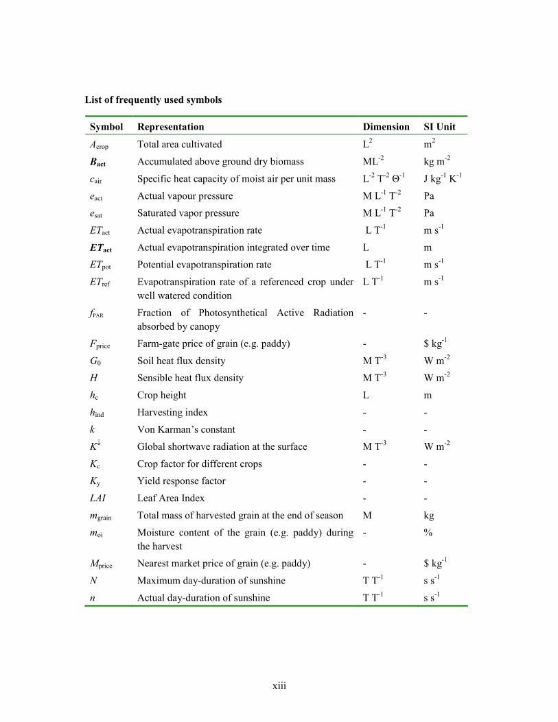
List of frequently used symbols

Symbol Representation Dimension SI Unit

Acrop Total area cultivated L2 m2

Bact Accumulated above ground dry biomass ML-2 kg m-2

cair Specific heat capacity of moist air per unit mass L-2 T-2 Θ-1 J kg-1 K-1

eact Actual vapour pressure M L-1 T-2 Pa

esat Saturated vapor pressure M L-1 T-2 Pa

ETact Actual evapotranspiration rate L T-1 m s-1

ETact Actual evapotranspiration integrated over time L m

ETpot Potential evapotranspiration rate L T-1 m s-1

ETref Evapotranspiration rate of a referenced crop under well watered condition

L T-1 m s-1

fPAR Fraction of Photosynthetical Active Radiation absorbed by canopy

- -

Fprice Farm-gate price of grain (e.g. paddy) - $ kg-1

G0 Soil heat flux density M T-3 W m-2

H Sensible heat flux density M T-3 W m-2

hc Crop height L m

hind Harvesting index - -

k Von Karman’s constant - -

K↓ Global shortwave radiation at the surface M T-3 W m-2

Kc Crop factor for different crops - -

Ky Yield response factor - -

LAI Leaf Area Index - -

mgrain Total mass of harvested grain at the end of season M kg

moi Moisture content of the grain (e.g. paddy) during the harvest

- %

Mprice Nearest market price of grain (e.g. paddy) - $ kg-1

N Maximum day-duration of sunshine T T-1 s s-1

n Actual day-duration of sunshine T T-1 s s-1

xiv


NDVI Normalized Difference Vegetation Index - -

P Precipitation on the gross command area L T-1 m s-1

Pe Effective Precipitation, derived from actual precipitation on the gross the command area, for the use of crop growth

L T-1 m s-1

Pe,ant Effective Precipitation, derived from Anticipated rainfall (predicted by past records) on the command area, for the use of crop growth

L T-1 m s-1

r0 Surface albedo - -

ra,h Near-surface aerodynamic resistance for heat transport

L-1T s m-1

rc Canopy resistance L-1T s m-1

rc,min Minimum value of the canopy resistance i.e. when soil water is not limited

L-1T s m-1

Rn Net radiation flux density: Rn = G0 + H + λET M T-3 W m-2

Rprice Price ratio: farm gate price of grain in terms of

nearest market price: price

priceprice

M

FR =

- -

t Time T s

Vc Actual irrigation water supply from the main source (e.g. reservoir, river diversion) to a command area

L T-1 m s-1

Vc,int Intended irrigation water supply from the main source (e.g. reservoir, river diversion) to a command area

L T-1 m s-1

Vdr Water discharged to the drainage canal system L T-1 m s-1

WPm,ET Productivity of Water determined by total Mass of grain Yield (seasonal) in terms of ETact:

act

grainETm,

ETm

WP =

ML-3 kg m-3

Yact Actual grain yield (paddy): cropgrain

act Am

Y = ML-2 kg m-2

Ymax Maximum attainable grain yield (paddy) ML-2 kg m-2

zoh Roughness length for heat transport L m

xv


zom Roughness length for momentum transport L m

∆v Slope of the vapor pressure curve - Pa K-1

ε Light use efficiency of crop L-2 T2 kg J-1

εapp Application efficiency of the available water for crop in the command area

- -

εcon Conveyance efficiency of the main canals in the irrigation system

- -

εdis Distribution efficiency of the distributary canals in the irrigation system

- -

γ Psychrometric constant L-1 M T-2 Θ-

1 Pa K-1

Λ Evaporative fraction: HR

λETGR

λETΛ+

=−

=n0n

- -

λ Latent heat of vaporization L2 T-2 J kg-1

λET Latent heat flux density M T-3 W m-2

ρair Air density ML-3 kg m-3

ρw Density of water ML-3 kg m-3

1. Introduction

1.1 Water for irrigated agriculture

By the year 2025, 83 % of the expected global population of 8.5 billion is expected to be live in developing countries. Yet the capacity of available resources and technologies to satisfy the demands of this growing population for food and other agricultural commodities remains uncertain. The world's food production depends on the availability of water, a precious but finite resource. The role of water as a social, economic, and life-sustaining good should be reflected in demand management mechanisms and be implemented through resource assessment, water conservation and reuse (UNCED, 2002). In Asia, irrigated agriculture produces rice as the major food crop because it is the region’s staple food. Asian countries dominate the world’s rice production (Fig. 1.1) controlling 90 % of the total with South Asia1 contributing 31 % (FAO_RAP, 2004). The challenge for irrigated agriculture today is to contribute to the world’s food production and to improve food security through more efficient and effective use of water.

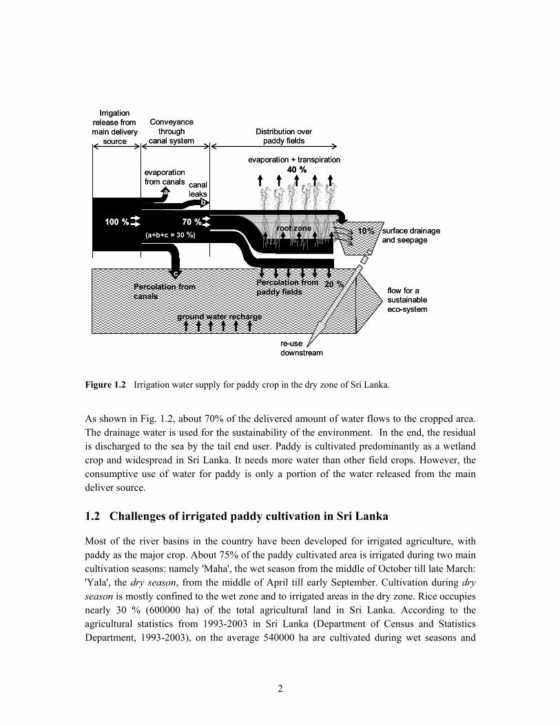
Water demands are increasing rapidly and thereby, available water for agriculture is getting limited. However within a river basin water is used by numerous of users (e.g. upstream nature, storage, irrigated and rain-fed agriculture, industries, and downstream wetlands). The only “volume of water” leaving the basin is the actual evapotranspiration which is the consumptive use of water and discharge to the ocean. Also, in irrigation systems for paddy cultivations consumptive use of water is about 40 % of the amount of water delivered to the cropped area from the reservoir or a river diversion (Fig. 1.2).

Figure 1.1 Average distribution of world’s rice production from 1993-2003

1 India, Pakistan, Sri Lanka, Bangladesh, Nepal, Bhutan and Maldives

9.5% (Rest of the World)

31% (South Asia)

59.5% (Rest of the Asia )

2

Figure 1.2 Irrigation water supply for paddy crop in the dry zone of Sri Lanka.

As shown in Fig. 1.2, about 70% of the delivered amount of water flows to the cropped area. The drainage water is used for the sustainability of the environment. In the end, the residual is discharged to the sea by the tail end user. Paddy is cultivated predominantly as a wetland crop and widespread in Sri Lanka. It needs more water than other field crops. However, the consumptive use of water for paddy is only a portion of the water released from the main deliver source.

1.2 Challenges of irrigated paddy cultivation in Sri Lanka

Most of the river basins in the country have been developed for irrigated agriculture, with paddy as the major crop. About 75% of the paddy cultivated area is irrigated during two main cultivation seasons: namely 'Maha', the wet season from the middle of October till late March: 'Yala', the dry season, from the middle of April till early September. Cultivation during dry season is mostly confined to the wet zone and to irrigated areas in the dry zone. Rice occupies nearly 30 % (600000 ha) of the total agricultural land in Sri Lanka. According to the agricultural statistics from 1993-2003 in Sri Lanka (Department of Census and Statistics Department, 1993-2003), on the average 540000 ha are cultivated during wet seasons and

re-use downstream

surface drainage and seepage

flow for a sustainable eco-system

Irrigation release from main delivery

source

Conveyance through

canal systemDistribution over

paddy fields

evaporation + transpiration

10%

canal leaks

40 %

(a+b+c = 30 %)

ab

100 %

evaporation from canals

root zone70 %

cPercolation from paddy fields

20 %

ground water recharge

Percolation from canals

re-use downstream

surface drainage and seepage

flow for a sustainable eco-system

Irrigation release from main delivery

source

Conveyance through

canal systemDistribution over

paddy fields

evaporation + transpiration

10%

canal leaks

40 %

(a+b+c = 30 %)

ab

100 %100 %

evaporation from canals

root zone70 %70 %

cPercolation from paddy fields

20 %

ground water recharge

Percolation from canals

3

320000 ha during dry seasons. Since 1977, about 155000 ha of paddy lands were developed under large-scale irrigation development programs launched in the country and the total rice production was also increased by 100% (Fig. 1.3).

About 1.8 million farm families are engaged in paddy cultivation island-wide. Sri Lanka currently produces 2.7 106 ton of rice annually and manages to satisfy around 95 % of the domestic requirement. The per capita consumption of rice fluctuates around 100 kg a-1 depending on the price of rice, bread and wheat flour. However, to meet the growing needs of the population, it is necessary to produce more in the future. New irrigation developments can be proposed to increase total production. Since land and water are becoming scarce resources against the increasing demand, such proposals are less feasible. However in 2000, the national annual average yield of rice (3700 kg ha-1) was around 50 % of the genetic potential of improved cultivars recommended for use in Sri Lanka. The predicted national average yield for the year 2005 was 4100 kg ha-1 (Dhanapala, 2000).

This situation shows that to increase the yield nearly by 50% over the existing paddy lands with available water, the productivity of paddy cultivation needs to be improved. In the irrigation sector, demand management stresses making on better use of existing supplies, rather than planning new developments. Irrigated agriculture has to meet this challenge by increasing the productivity of water, land, and other input commodities already in use.

Figure 1.3 Trend of annual paddy production and annual grain yield in Sri Lanka from 1952-2003. Source: Department of Census and Statistics, Sri Lanka (1952-2003).

0.0

0.5

1.0

1.5

2.0

2.5

3.0

3.5

4.0

1952

1955

1958

1961

1964

1967

1970

1973

1976

1979

1982

1985

1988

1991

1994

1997

2000

2003

Ann

ual p

addy

pro

duct

ion

(10

6 ton)

0

500

1000

1500

2000

2500

3000

3500

4000

Ann

ual g

rain

l yie

ld Y

act (

kg h

a-1)Annual paddy production

Annual grain yield of paddy

4

1.3 Water in dry zone areas and irrigation for paddy

Most of the irrigation schemes are located in the dry zone where expected water demand is much higher than what is received from monsoon rains. The lower part of the catchment receives an annual rainfall of less than 900 mm. During the wet season, most of the rainfall falls in a few very intensive storms, which result in only a partial storage in irrigation reservoirs. Thus, water availability has become a critical issue in the dry zone of Sri Lanka.

There are two types of irrigation schemes in the country, namely reservoir schemes and diversion weir schemes. In case of significant areas, additional reservoirs are constructed within the irrigation system for water storage. In a river basin, most of the irrigation schemes located one downstream of the other in the form of cascade, reusing drainage water from the schemes upstream.

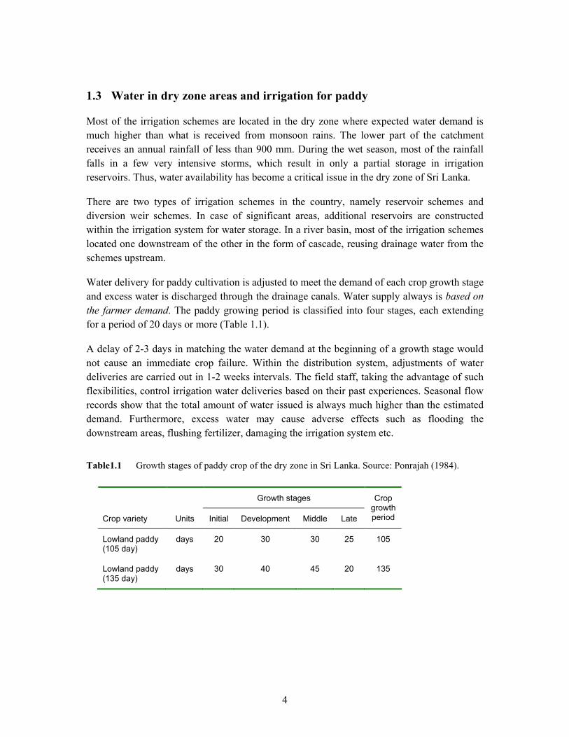
Water delivery for paddy cultivation is adjusted to meet the demand of each crop growth stage and excess water is discharged through the drainage canals. Water supply always is based on the farmer demand. The paddy growing period is classified into four stages, each extending for a period of 20 days or more (Table 1.1).

A delay of 2-3 days in matching the water demand at the beginning of a growth stage would not cause an immediate crop failure. Within the distribution system, adjustments of water deliveries are carried out in 1-2 weeks intervals. The field staff, taking the advantage of such flexibilities, control irrigation water deliveries based on their past experiences. Seasonal flow records show that the total amount of water issued is always much higher than the estimated demand. Furthermore, excess water may cause adverse effects such as flooding the downstream areas, flushing fertilizer, damaging the irrigation system etc.

Table1.1 Growth stages of paddy crop of the dry zone in Sri Lanka. Source: Ponrajah (1984).

Growth stages

Crop variety Units Initial Development Middle Late

Crop growth period

Lowland paddy (105 day)

days 20 30 30 25 105

Lowland paddy (135 day)

days 30 40 45 20 135

5

Hence, a proper water management system based on crop water demand and the farming practices is of great importance to guide the irrigation field staff. In order to achieve this, it is necessary to have a reliable criterion to assess the performance of the scheme at regular intervals.

1.4 Problem statement

To increase the productivity of paddy through improved management of the available resources, the national goals are specified. In the goal achieving process, performance of the irrigated agriculture process determines whether the targets are attained. Performance assessment from the operational level of the scheme up to the national level is of prime importance. Hence, it is necessary to evaluate whether the current performance assessment program can assess the performance of the schemes as well as the irrigated agriculture sector. In most of the irrigation schemes, seasonal performance is quantified only at the end of the season (Table 1.2).

The indicators shown in Table 1.2 measure the productivity of water in terms of irrigated land area, seasonal grain yield, and the district level rice production contributes to fulfill the national demand, respectively. Seasonal records of these measurements are maintained. Associated with other regular field measurements, the water managers compare the seasonal grain yield with the past records in order to make certain decisions about the forthcoming season, e.g. water adequacy, extent to be cultivated, suitable crop type and variety.

Table 1.2 Currently used performance indicators. Note: Measurements denoted by * are taken through sample surveys.

Relationship Performance indicator Units

Irrigation requirement cultivated area Total

supply irrigation Actual

crop

c AV

= m3 ha-1

Grain yield Yact

cultivated area Total grain harvested of mass *Total

crop

grain A

m= ton ha-1

District level grain yield *District level grain yield through statistical analysis

ton season-1

6

However, these indicators are susceptible to unusual weather conditions e.g. a long unexpected drought or excessive rainfall. Neither do they review the operational performance of the system e.g. identification of crop water stressed areas. Performance information on related activities (e.g. water delivery, drainage control, water shortage) is required by the operational managers on time to make relevant decisions. Also, productivity can be increased only by the effective use of input resources such as, water, land, labor, infrastructure, money etc.

Water managers of an irrigation scheme should monitor the performance of key operations closely to identify shortcomings and take corrective measures at the right time. Performance assessment provides relevant feedback controls to the management, where as performance indicators provide necessary information for those controls. A reliable performance assessment criterion requires a comprehensive study of the system, considering present management practices and associated boundary conditions. A performance indicator is set to a target level with an allowable range of deviation (tolerance margin) depending on the local boundary conditions. Continuous observations of the indicator value in close intervals indicate the output level variation against the target value (Fig.1.4). The indicator can fluctuate within the allowable range without triggering a management action. However, if the indicator moves out of this range, diagnosis of the problem should lead to the planning of corrective action.

Figure 1.4 Terminology on the use of performance indicators Source: Bos et al. (2005)

Target level

Valu

e of

per

form

ance

indi

cato

r

tolerance margin

impact of corrective action

Time

planning for corrective action

corrective action taken

Highest attainable level

critical deviation

Target level

Valu

e of

per

form

ance

indi

cato

r

tolerance margin

impact of corrective action

Time

planning for corrective action

corrective action taken

Highest attainable level

critical deviation

7

Performance gap, the deviation of the actual performance from the target level, is the determination of low performance. However, prior to take corrective measures, the cause for low performance needs be diagnosed. For example, taking one indicator used at present: irrigation requirement may show a relatively higher value than that of near past years. There may be several possible causes for low performance (Fig. 1.5) and to take corrective measures is not possible until the root causes are correctly identified.

By incorporating with some other indicators related to the possible causes, the root causes could be identified through a diagnostic approach. The rationale behind performance assessment is to diagnose any performance gap in the goal achieving process and to rectify the situation. Hence, managers at different levels should identify the performance gap (if any), find the cause for the gap, and take corrective measures to cure the below target performance. Therefore, a suitable performance assessment criterion has to be developed and assured. Also, appropriate performance indicators to assess the performance of the scheme have to be identified.

To assess performance, objective data on actual field performance is needed, but unavoidable time delays in this process cause delays in the decision making process. In order to make decisions at the right time, the delays of acquiring and processing of field data should be minimized. Satellite remote sensing can furnish near-real time data in an objective and unbiased manner.

.

Figure 1.5 Possible causes encountered while diagnosing to find the root-cause for low performance.

ProblemRelatively high

value of Irrigation requirement

Poorcontrol of water by

operational staff

Extended time for land preparation

(lack of machinery)

Seed paddy with extensive growth period

Poor scheduling

of water deliveries

Possible causes

ProblemRelatively high

value of Irrigation requirement

Poorcontrol of water by

operational staff

Extended time for land preparation

(lack of machinery)

Seed paddy with extensive growth period

Poor scheduling

of water deliveries

Possible causes

8

The use of remote sensing has several distinct advantages over traditional field data collection. Remote sensing can be used to gather information over an entire area, while field data collection relies on sample areas (e.g. sample survey for crop cutting data, crop evaporation using evaporation pan). Hence, the amount of field data can be reduced by the use of satellite remote sensing. The improved facilities of satellite remote sensing can now provide information on daily basis with the spatial resolution of 250 m to 1000 m.

1.5 Opportunities of remote sensing for irrigation performance

The potentiality of remote sensing techniques in irrigation and water resource management has been widely acknowledged. Environmental physics based on electromagnetic radiation and micro-hydrology has evolved in the development of quantitative algorithms to convert remotely sensed spectral radiances into useful information such as evapotranspiration, root zone soil moisture, and biomass growth. Estimation of crop water parameters using remote sensing techniques is an expanding research field and development trends have been progressing since 1970s (e.g. Hiler and Clark, 1971; Jackson et al., 1977; Seguin and Itier, 1983). The remote sensing algorithms such as SEBAL (Surface Energy Balance Algorithm for Land) by Bastiaanssen et al. (2003) and SEBS (Surface Energy Balance System) by Su (2002) are currently used approaches to estimate crop water parameters. Different applications relating crop water consumption to irrigation water supply by remote sensing (e.g. Roerink et al., 1997) with developed theories are available in the electronic media with easy access. Also, in the field of geoinformatics, the software developments provide advanced techniques and modern facilities to the user. The low cost high speed personal computers can handle vast amounts of data at a time.

The remote sensing technology is widespread in Sri Lanka, but it has rarely been applied to support irrigation management practices probably because of the associated costs and lack of transferred technology. Prices are decreasing rapidly, and the quality of images is improving.

The scale of satellite measurements is a measure of its quality and which is associated with two parameters, namely spatial resolution and temporal resolution. The spatial resolution measures the ability of a sensor to distinguish among closely spaced objects in the terrain. One pixel is the smallest area of the terrain that can be recorded as a unique element by the sensor. Ground objects smaller than the pixel size can be detected but not be resolved. In a satellite image, a ground object of whatever shape has to be identified approximately by a cluster of square shaped pixels i.e. a raster based image (Table 1.3).

9

Table 1.3 The main characteristics of the satellites considered for the study.

Characteristics Unit Landsat-7 ETM+ ASTER NOAA-AVHRR MODIS

Platform/Sensor - Landsat Enhanced Thematic Mapper Plus

Advanced Space-borne Thermal Emission and Reflection Radiometer

National Oceanic and Atmospheric Administration-Advanced Very High Resolution Radiometer

Moderate Resolution Imaging Spectroradiometer

Type High resolution High resolution Low resolution Low resolution

Orbital altitude km 705 705 833 705

Image coverage km 185 60 2399 2330

Temporal resolution d 16 16 0.5 1

Equator crossing time hrs (local) 10:00 10:30 2:30 and 14:30 10:30

Visible detectors

Band numbers - 1- 4 1-2 1 1, 3, 4 and 8 - 14

Spectral range µm 0.45 – 0.69 0.52 – 0.69 0.58 – 0.68 0.545 – 0.670

Spatial resolution m 30 15 1100 250 (band 1)

500 (band 3 and 4)

1000 (band 8 – 14)

10

Table 1.3 continued.

Characteristics Unit Landsat-7 ETM+ ASTER NOAA-AVHRR MODIS

Infrared detectors

Band numbers - 4,5 and 7 3 - 9 2 - 3 2, 5-7, and 15 - 30

Spectral range µm 0.76 - 2.35 0.76 – 2.43 0.725 – 3.93 0.62 – 9.88

Spatial resolution m 30 15 (band 3)

30 (band 4 – 9)

1100 250 (band 2)

500 (band 5 - 7)

1000 (band 15 – 30)

Thermal detectors

Band numbers - 6 10 - 14 4 - 5 31 - 36

Spectral range µm 10.4 – 12.5 8.125 – 11.65 10.3 – 12.5 10.78 – 14.385

Spatial resolution m 60 90 1100 1000

11

Images from satellites such as Landsat-7 ETM+ or ASTER produce a more accurate shape of the ground object because of their smaller pixel size (e.g. 30 m × 30 m), compared to those of the MODIS or the NOAA-AVHRR satellites which have pixels of 1000 m × 1000 m and 1100 m × 1100 m respectively. While checking high spatial resolution satellite images such as ASTER or Landsat-7 ETM+, in several ASTER images it was found that the sensor has scanned only a part of the study area. This is because of the narrow coverage of the ASTER scanner (60 km) and its specified path along the study area. This problem has not seriously arisen in the Landsat-7 ETM+ images.

The temporal resolution determines the frequency of revisits of the satellite to capture images of the same area. In practice, the frequency of image capture could be hampered by cloud cover, which makes the measurements useless. Both the Landsat-7 ETM+ and the ASTER satellites have a 16 day temporal resolution, meaning even if there would be no cloud cover, they could provide only 2 measurements of a particular area per month. In comparison, the MODIS and the NOAA-AVHRR satellites provide daily measurements.

Now, the growing period of the recommended paddy crop in Sri Lanka varies from 105 days to 120 days, and the field conditions need to be monitored in intervals at least of 10 days. Thus, the MODIS or the NOAA-AVHRR can provide images within the required monitoring frequency, even allowing for certain amount of cloudy days. In addition, its images are freely available through internet, the only cost being that of downloading them. For this study, both satellites can provide measurements with similar characteristics. The MODIS images have a minor advantage of the spatial resolution. The MODIS images were selected for the study. If MODIS images can be used to measure parameters with sufficient accuracy, a cost effective tool could be developed to support strategic management decisions.

12

1.6 Outline of the thesis

The main objective of this study is to develop and introduce a cost effective performance assessment program to manage irrigation systems using satellite remote sensing as a tool and to assess whether the results are sufficiently accurate to support the managerial decisions at all levels.

The specific research objectives of this study are:

• To develop an approach to select most relevant performance indicators from the published long lists to assess irrigation performance.

• Error estimation of evapotranspiration derived from remote sensing model due to changes in ground cover.

• Determination of the effectiveness of remotely sensed data in combination with regular flow measurements in improving productivity of irrigation schemes in Sri Lanka.

Chapter 2 describes the study area, the Uda-Walawe irrigation scheme and the Liyangastota irrigation scheme of Walawe rive basin. In addition, this chapter describes the topography, irrigation and drainage system, hydrology, and the land-use soil types of the study area. Important issues related to the present irrigation management practices, framers’ current position in the field of irrigated agriculture, and their potential needs are discussed in the end.

Chapter 3 presents the framework of performance assessment for the study area based on the management practices of the irrigated agriculture sector in Sri Lanka. Major aspects of irrigated agriculture are specified based on the role of water institutions and related boundary conditions. An approach is proposed for selecting relevant performance indicators from the published long lists. An appropriate set of performance indicators are selected by considering the facilities of satellite remote sensing and other feasible local conditions.

Chapter 4 describes the remote sensing approach used for the estimation of parameters required for the performance assessment. The SEBAL model is applied for the MODIS satellite measurements having 1000 m × 1000 m spatial resolution. The critical issues of applying the SEBAL model are discussed. A remote sensing model relating reflectance data is explained for estimating accumulated biomass and thereby, to predict seasonal grain yield of paddy.

Chapter 5 estimates the error of actual evapotranspiration due to the spatial scale of the MODIS images (1000 m × 1000 m) compared to the 30 m × 30 m resolution Landsat-7 ETM+ images. To assess the error component of actual evapotranspirtaion while increasing the spatial extent of the ground cover, an approach is developed. Impact of boundary pixels as well as the heterogeneity of the land cover on actual evapotranspiration is considered. By

13

considering the trend of the error component of actual evapotranspiration, a feasible spatial extent for the MODIS measurements is recommended.

In Chapter 6 two examples of assessing operational irrigation performance of the Liyangastota right bank system, is assessed using selected indicators for water balance: one for a wet season and the other for a dry season. The target level and the critical level of the indicators are determined. To assess the variations of the crop water stress with the irrigation water deliveries, a water use matrix for irrigated crops is introduced. To assess the irrigation performance, the growth period of paddy is divided into 10 day intervals.

In Chapter 7 the socio-economic performance is assessed for all four sub-schemes in the study area. The indicators are seasonal grain yield, water productivity, and price ratio. Seasonal grain yield is compared with the measurements of crop cutting surveys in the area. The time factor and the cost factor of using satellite remote sensing for performance assessment are discussed. In addition, institutional settings required for the implementation of performance assessment in the Irrigation Department of Sri Lanka are discussed and recommendations are made.

15

2. Description of the study area

2.1 Introduction

The study area, Uda_Walawe and Liyangastota irrigation schemes, is located in the South-east dry zone of Sri Lanka. The main water source for these irrigation schemes is the river Walawe, which has the largest river basin in this part of the country. This river originates at the southern edge of the central massif at a relatively high elevation of around 1800 m, above MSL and traverses about 136 km before it reaches the ocean. The Walawe river basin falls approximately between latitudes 6.110 and 6.840 and longitudes 80.570 and 81.020. The catchment of the basin amounts to 2442 km2 and extends about 57 km east to west and 82 km from north to south (Fig. 2.1).

Figure 2.1 Geographical location and main features of the study area: a) Walawe river basin and the study area located in a river basin map of the country, and b) details of the study area and the river basin.

Weather station at Angunakolapelessa

Colombo

Trincomalee

HambantotaIndian ocean

Reservoir dam

Walawe river basinStudy area

Uda_Walawereservoir

Walawe river

Sevanagala

Command area

Ridiyagamareservoir

Liyangastotariver diversion

Rakwanariver

a b

Sea

N

0 20 40 km 0 12 km

Weather station at Angunakolapelessa

Colombo

Trincomalee

HambantotaIndian ocean

Reservoir dam

Walawe river basinStudy area

Uda_Walawereservoir

Walawe river

Sevanagala

Command area

Ridiyagamareservoir


Rakwanariver

a b

Sea

N

0 20 40 km0 20 40 km 0 12 km0 12 km

16

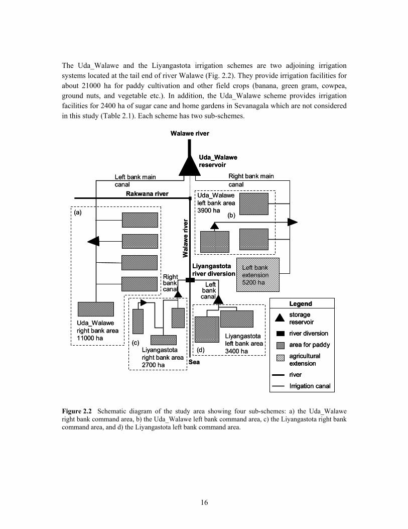
The Uda_Walawe and the Liyangastota irrigation schemes are two adjoining irrigation systems located at the tail end of river Walawe (Fig. 2.2). They provide irrigation facilities for about 21000 ha for paddy cultivation and other field crops (banana, green gram, cowpea, ground nuts, and vegetable etc.). In addition, the Uda_Walawe scheme provides irrigation facilities for 2400 ha of sugar cane and home gardens in Sevanagala which are not considered in this study (Table 2.1). Each scheme has two sub-schemes.

Figure 2.2 Schematic diagram of the study area showing four sub-schemes: a) the Uda_Walawe right bank command area, b) the Uda_Walawe left bank command area, c) the Liyangastota right bank command area, and d) the Liyangastota left bank command area.

Walawe river

Uda_Walawereservoir

Wal

awe

river

Left bank extension 5200 ha

Right bank canal


Right bank main canal

Left bank main canal

Rakwana river

Left bank canal

Uda_Walaweright bank area 11000 ha

Liyangastotaright bank area 2700 ha

Liyangastotaleft bank area 3400 ha

Uda_Walaweleft bank area 3900 ha

Sea

storage reservoir

river diversion

area for paddy

agricultural extension

river

Irrigation canal

Legend

(a) (b)

(d)(c)

Walawe river

Uda_Walawereservoir

Wal

awe

river

Left bank extension 5200 ha

Right bank canal


Right bank main canal

Left bank main canal

Rakwana river

Left bank canal

Uda_Walaweright bank area 11000 ha

Liyangastotaright bank area 2700 ha

Liyangastotaleft bank area 3400 ha

Uda_Walaweleft bank area 3900 ha

Sea

storage reservoir

river diversion

area for paddy


river

Irrigation canal

Legendstorage reservoir

river diversion

area for paddy


river

Irrigation canal

Legend

(a) (b)

(d)(c)

17

Table 2.1 Cropping pattern under the Liyangastota and the Uda_Walawe irrigation schemes during the research period. Source: Field offices of the Uda_Walawe scheme and the Liyangastota scheme.

Liyangastota Uda_Walawe

Right bank Left bank Right bank Left bank

Season Paddy Paddy Paddy Sugar Others Paddy Sugar Others

2002-2003 wet

2725 3440 6660 86 4141 2166 1911 1631

2003 dry 2725 3440 7404 172 3966 2185 1911 1328

2003-2004 wet

2725 3440 6785 172 4303 1994 1911 1509

2.2 Historical development of the study area

The Uda_Walawe multipurpose reservoir project was started in 1963, with land development for irrigated agriculture as the main objective. Construction works as well as water management activities were carried out by the River Valleys Development Board (RVDB), a state sector construction agency. The main structure of the Uda_Walawe reservoir, the 4 km long and 36 m earth-filled dam across the river was completed in 1967. The live storage of the reservoir is 269 106 m3 and provides irrigation facilities through two irrigation canals running either sides of the river. Only a part of the drainage discharge of the scheme reaches the main river course. The proposed plan anticipated that the Uda_Walawe reservoir would provide sufficient water to irrigate a command area of about 33000 ha with a cropping pattern of 14000 ha of rice, 7300 ha of sugar, and 11700 ha of cotton and non-rice crops.

While carrying out the construction works for the downstream development of the scheme, cultivation was started in the already completed part of the command area. With lack of marketing channels, and inexperience with non-rice crops, the farmers opted for what they perceived as the least risky approach. They focused exclusively on rice production. This resulted in higher water usage than anticipated. The right bank area envisioned for irrigation was consuming 3 times the water budgeted (ADB, 1979). Because of this further development of the left bank was curtailed.

In 1987, due to poor performance, the management of the project was handed over to the Mahaweli Authority of Sri Lanka2, another state sector organization. The cultivated area of the right bank was about 10500 ha out of 12000 ha of potential area. In the left bank area about 4000 ha was cultivated with paddy in addition to 2000 ha of sugar cane. In a relatively 2 Mahaweli Authority of Sri Lanka manages several irrigation schemes in selected river basins.

18

short period of time, the Mahaweli Authority increased the paddy yield from 3.6 ton ha-1 to 4.0 ton ha-1. However, the project was yielding only about 60% of the estimated benefits (Molle and Renwic, 2005). In 1988, Mahaweli Authority began a crop diversification program. About 5 % to 6% of the command area was cultivated with non-rice crops. However, banana cultivation was gradually increased over the highlands of the command area. Cultivation of banana and non-rice crops were sparsely scattered over the command area. Literature shows that banana cultivation is reached about 4000 ha in the command area (Molle and Renwic, 2005). An accurate land survey has yet to be carried out to determine the actual cultivated area of rice and non-rice crops. At present, the command area has increased to 11,000 ha in the right bank and 6400 ha in the left bank.

In 1991, Japan International Cooperation Agency (JICA), working along with the Mahaweli Authority, conducted a feasibility study for agricultural development in the left bank area. The overriding objective was to increase agricultural production and water use efficiency and to use resulting water savings for the development of further 5200 ha of the left bank area. The rehabilitation program was over in 2003. The development of left bank extension is now in progress.

Under the water resource development program of Walawe river basin, Liyangastota diversion weir was completed in 1889 and the down stream development of the right bank and the left bank canals were completed in 1928. Its 73 m long diversion weir is located at Liyangastota, 21 km upstream of the sea outfall of the river Walawe and 30 km downstream of Uda_Walawe dam. Water is diverted for irrigation through canals on both river banks. The left bank canal feeds the Ridiyagama storage reservoir before issuing water to the irrigation system. The right bank canal issues irrigation water directly from the river flow. There are two small storage reservoirs along the right bank main canal to stabilize the canal flow. At present, the command area has increased to 2700 ha in the right bank and 3400 ha in the left bank.

A part of the drainage discharge from Uda_Walawe is tapped by Liyangastota scheme, but its main source of water is the Rakwana River, a tributary of Walawe which joins the main river at immediate downstream of the Uda_Walawe reservoir as shown in Fig. 2.2.

Since the construction, no complete rehabilitation has been done in the canal system. However, urgent rehabilitation works, repairs and modifications have been carried out under routine maintenance programs. In 1994, JICA carried out a feasibility study on rehabilitation of the Liyangastota scheme. The yield standard was estimated as 3.4 ton ha-1 and cultivation of non-rice crops was found as minimal (JICA, 1996). The study report indicates the requirement of a complete rehabilitation program in order to improve the cropping intensity and the productivity of paddy cultivation. The proposed rehabilitation program of the Liyangastota scheme was commenced in year 2000. Prior to rehabilitation, due to poor

19

condition of the flow measuring structures, canal erosions, and sedimentation, it was not possible to launch an effective water management program.

2.3 Climate and weather

As in the rest of the country, the climate of the dry zone is classified as a tropical monsoon climate with two distinguished monsoons (South-West monsoon and North-East monsoon). Hence, rainfall in the Walawe basin is bi-model with precipitation occurring during two seasons each year: the South-West monsoon season from May to September and the North-East from December to February. The annual rainfall in the upper part of the study area had been fluctuating around 1500 mm (Fig. 2.3a). But a declining trend can be seen since last three decades. In the lower part of the study area, annual rainfall fluctuates around 1000 mm, also with a declining trend (Fig. 2.3b).

The monthly rainfall distribution over the basin (Fig. 2.4) reveals that the study area receives less rainfall than the average for the entire basin. The daily mean temperature of the study area varies from 240 C to 320 C. During the hot periods, from March to April and from August to September, daily maximum temperature rises from 330 C to 380 C. During the cooler period, from December to January, daily minimum temperature fluctuates around 200 C.

20

Figure 2.3 Annual rainfall of the study area from 1960 to 1999: a) upper part of the study area, and b) lower part of the study area. Source: The IWMI database on the Ruhuna basin (2005).

The Meteorology Department of Sri Lanka has established weather stations island-wide and records are maintained on hourly basis. Air temperature (maximum, minimum, and average), wind speed, sun shine records, relative humidity, and rainfall records were collected for this study from the weather stations close to the study area. The Angunakolapelessa weather station is located within the study area and two others are located at dam of the Uda_Walawe reservoir and Sevanagala as shown in Fig. 2.1b. Additionally, few rain gauges are fixed at selected places over the command area.

0

500

1000

1500

2000

2500

1960

1962

1964

1966

1968

1970

1972

1974

1976

1978

1980

1982

1984

1986

1988

1990

1992

1994

1996

1998

Rai

nfal

l (m

m)

declining trend

0

500

1000

1500

2000

2500

1960

1962

1964

1966

1968

1970

1972

1974

1976

1978

1980

1982

1984

1986

1988

1990

1992

1994

1996

1998

Rai

nfal

l (m

m)

declining trend

(a)

(b)

21

Figure 2.4 Spatial distribution of average monthly rainfall from 1961 to 1990. Source: Jayathilake (2002) and the IWMI database on the Ruhuna basin (2005).

2.4 Land use

According to the map of Agro-ecological regions of Sri Lanka (Dept. Agri., 2003), the soil groups are similar in the upper and lower parts of the study area despite the variation in rainfall. In the lower region, soil groups (for land use) are RBE (Reddish Brown Earths), LHG (Low Humic Gley soils)3 and Alluvial soils. These soil groups occur in gently undulating terrain and in the river flood plains and belong to different drainage and textural classes. RBE soils within the irrigation schemes are confined to paddy cultivation and could be used for rice during both seasons. Rice growing LHG soils are confined to the valley bottoms of the undulating terrain. The main soil groups in the upper region are also RBE and LHG, but drainage classes differ from well-drained to poorly-drained. The Agriculture Department reports that under good management control of both irrigation and agricultural aspects, a paddy yield of 6000 kg ha-1 to 8000 kg ha-1 can be expected from these soil classes in either season (Dept. Agri., 2003).

3 According to the ASTM-D 2487 (American Society for Testing and Materials), RBE is classified as SC (Clayey Sand) and LHG is classified as CL (Lean Clay) with the group name of Sandy Lean Clay

0

50

100

150

200

250

300

350

Jan

Feb

Mar

Apr

May

Jun

Jul

Aug

Sep Oct

Nov

Dec

Ave

rage

rain

fall

(mm

mon

th-1)

Walawe basinStudy area (upper part)Study area (lower part)

22

2.5 Irrigation management

In both schemes under study, seasonal water distribution schedules are prepared considering potential crop water demands and anticipated conveyance losses. Water distributions are managed by the field staff up to the secondary level and the farmer organizations are responsible for the tertiary level distributions. During the short fallow period between each cultivation season, the Irrigation Department carries out the routine maintenance of the irrigation system excluding the field canals (tertiary level).

Water allocations are computed on the basis of the growth stages shown in Table 1.1. For the dry zone of Sri Lanka, monthly evapotranspiration values of a referenced crop have been computed with respective crop factors. Irrigation efficiencies of different canal systems and anticipated monthly rainfall values are used for the computation of irrigation water requirements (Ponrajah, 1984). Recently, lined sections of the main canal were calibrated against the water depth. To adjust the water deliveries, these pre-computed flow ratings against the gauge heights are used by the field staff. To regulate the main canal flow, manually operated gates are adjusted. Each (lateral) distribution canal has an off-take structure with a manually operated flow control gate and a gauge fixed at the downstream canal section to measure the flow. Several (tertiary) field canals are connected to each distribution canal. Each field canal has a turn-out structure with a locking arrangement. At the field canal level, canal flows are not measured. The delivered water along the (lateral) distribution canal is distributed by the farmers. Daily gauge records are obtained by the field staff.

In both Uda_Walawe and Liyangastota irrigation systems, storage reservoirs are located along the main canals. Hence water deliveries are scheduled under the method of continuous flow system. However, irrigation water deficiencies have been reported from the tail end fields of both schemes because farmers at head reach of the canals tend to use more than their fair share of irrigation water by damaging hydraulic regulatory structures, canal banks and blocking the canal flow. Rotational water issues are started in such difficult areas. For paddy cultivation in the dry zone areas, rotational interval cannot be extended more than 3 to 4 days. However, for banana cultivation, the rotational interval can be extended more than 7 days. Because of this, farmers in the water shortage areas of the Uda_Walawe scheme have gradually turned into banana cultivation.

When cultivation starts, field officers have to use their own experience and skills to control the water distribution other than to stick to follow a planned process. Therefore, performance of canal operations is not assessed in a meaningful way as explained in the problem statement (section 1.4). Thus, operational controls are restricted only to find temporary solutions for emergencies, rather than to take corrective measures by diagnosing the situation. This situation becomes so critical during the dry periods that water managers are compelled to

23

provide additional water deliveries to save the crop. Through this practice hardly any improvement in performance can be expected.

Due to lack of proper controls, a huge amount of irrigation water is discharged into the drainage system; only a part of Uda Walawe drainage discharge is reused by Liyangastota scheme. Drain discharges, however, are not measured on a routine basis. As a result, the water balance of irrigated areas is inaccurate. The Liyangastota scheme does not receive a direct flow from Walawe river because of the reservoir upstream, but it does not suffer from water shortages because its main source, the Rakwana river (Fig. 2.2), has no storage facilities. Water development proposals of the Rakwana river are under investigation. One of the key proposals is to construct a new reservoir at the upstream of the Rakwana river basin which considers the water users of Rakwana river basin as the target beneficiaries. This proposal could restrict water inflow to the Liyangastota scheme. Furthermore, to irrigate additional 5200 ha in the Uda Walawe scheme left bank is currently in progress. This new extension is located in the lower part of the study area where the annual rainfall is less than 900 mm and the soil types are well drained RBE soils and poorly drained LHG soils. Some parts of this area are under rain fed cultivation during the wet season.

Having considered the soil types and the topography, less water consuming crops are recommended. With the extension, the total command area under both schemes increased by 25%. Thus, in the near future, only an effective and efficient water management strategy could assure the survival of these two irrigation schemes.

Since irrigation performance is assessed through this study, the next goal is to improve the productivity of other inputs. The outcomes of this study can be incorporated to assess the performance of other input needs such as quality of crop varieties (e.g. high yielding paddy), usage of fertilizer and other agro-chemicals, and water quality of drainage discharge etc. Also, this study computes the actual evapotranspiration, one of the water balance components. Hence, related to this study, modeling for ground water recharge would be a potential research area.

2.6 Farmer’s income and the productivity level of irrigated agriculture

During the last decade, production costs of paddy have increased tremendously though irrigation water is provided as a cost free service by the government. With the rapid increase in world’s oil prices and depreciation of local currency in the dollar market, prices of fertilizer and other agro-chemicals (i.e. petroleum by-products), and machinery hire charges have gone up. Daily labor charges also have gone up due to the increased cost of living. The subsidies provided by the government are not adequate to compensate the situation. The paddy cultivation is less labor intensive during the middle part of the season. The farmers engage in other small scale income generating activities during their free time. Also, the farmer knows

24

that the paddy cultivation ensures his domestic food supply. These reasons keep the Sri Lankan farmers stick to paddy cultivation though it brings low profits. On the other hand, the market price of rice has risen by 75% within the last 5 years due to high input costs and the consumers too cry out for government subsidies.

In this context, the paddy cultivating farmers need to receive more financial benefits for their existence where as the government need to ensure the food security of the country by eliminating any import bill for rice, as well as to protect the consumer. In order to make this situation stable, the irrigation and the agricultural authorities of the irrigated agriculture sector need to find feasible solutions. The crop diversification program has become one of the alternative solutions for the farmer community. Sri Lanka still imports other field crops such as chilies, onions, and cereals to meet the local demand. Most of the other field crops provide higher profits to the farmers than paddy. Well drained soils (e.g. RBE soils) are suitable for these crops and therefore the highland farmers have the advantage of crop diversification. However, the high capital investment associated with non-paddy crops and their continuous demand for labor compels the farmers not to commit them for crop diversification.

On the other hand, the local production costs of other field crops are high compared to neighboring countries and Sri Lanka cannot find an export market if the production of such crops exceeds the local demand. So, high yielding crop varieties suitable for local conditions need to be developed.

As another alternative, farmers of the South-east dry zone started cultivating banana in the highland areas because of its moderately low initial investment and considerably high profits. As a result of low interest credit facilities for banana cultivation introduced by some local investment banks, banana cultivation has been gradually picking up over the study area. An accurate survey has not yet been carried out to identify the correct extent of banana. At present, banana has a stable market in the area.

Under these circumstances, the most feasible option is to take adequate measures to increase the present yield level of paddy grain. Several pilot programs have been carried out by the Department of Agriculture in this context. Records of such a pilot project indicate that in the dry and wet seasons, the farmers were able to increase the average rice yield by 37% and 51 %, respectively (Table 2.2).

The yields could be increased by improving the technology as well as management practices. The Agriculture Department of the country has already introduced different high yield varieties to suit different environmental conditions of the country. Thus one can expect that with the existing technology, a grain yield of about 7 ton ha-1 is attainable in well managed irrigated paddy lands in the Dry zone of Sri Lanka.

25

Table 2.2 Average yield recorded (1998) with the implementation of the technological package in the dry zone of Sri Lanka, under major irrigation. Source: Dhanapala (2000).

Yield component of paddy Unit Wet season Dry season

Under normal management of irrigated agriculture

Average grain yield ton ha-1 4.66 3.90

With improved management of irrigated agriculture

Average grain yield ton ha-1 6.40 5.90

Average grain yield increased % 37 51

Highest grain yield ton ha-1 8.30 7.80

Highest grain yield increased % 78 96

Based on the attainable grain yield of 7 ton ha-1, seasonal grain yield of the Uda_Walawe scheme can be compared with the available past records (Fig. 2.5).Past records of the Liyangastota scheme are separately not available. Fig. 2.5 shows that the highest frequency level (4.8 ton ha-1) of the distribution of seasonal grain yield of paddy is below the attainable level.

Figure 2.5 Seasonal grain yield of paddy in the study area from 1979 to 2003. Source: The IWMI database on Ruhuna basin (2005).

0

1000

2000

3000

4000

5000

6000

7000

8000

1979

1981

1983

1985

1987

1989

1991

1993

1995

1997

1999

2001

2003

Sea

sona

l yie

ld (k

g ha

-1)

Wet seasonDry season

Highest frequency level of the distribution

Attainable level under improved management of irrogated agriculture

27

3. A new performance program for the study area

3.1 Management hierarchy of the irrigated agriculture sector in Sri Lanka

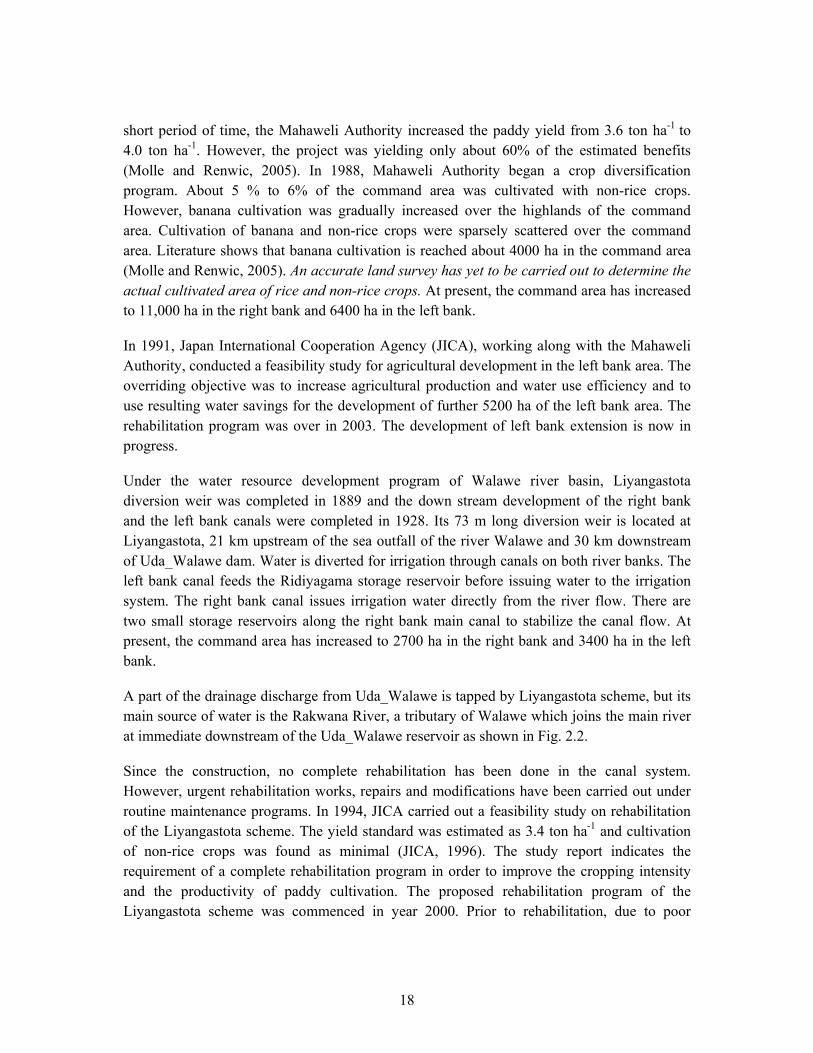
In Sri Lanka, the main objective of irrigated agriculture is to achieve self sufficiency through sustainable irrigation management while satisfying the farmer: the producer, the public: the consumer, and the environment: the agro eco-system. In the country, paddy cultivation forms the economy of the rural society and for the urban society it is the staple consumption. To achieve the national goals of rice production, the paddy cultivation is heavily subsidized by the Government. Coordinating with other organizations, the Irrigation Department implements the national cultivation program of paddy and other field crops. To formulate national policies related to the needs of irrigated paddy cultivation, information on current performance and the performance of the cultivation process are reviewed by the management at different levels of the management hierarchy (Fig. 3.1).

Figure 3.1 Management hierarchy of the irrigated agriculture sector in Sri Lanka.

Operationallevel

Tacticallevel

Strategiclevel

National economic plan

Ministries of theirrigated agricultural sector

Line organizations of the irrigated agriculture sector

[Irrig. Dept., Agri. Dept., etc.]

Offices of line organizations to regional level control[Regional officers, District secretary]

Field level operations [Field staff]

Offices of lineorganizations to divisional level operations[Divisional officers, Divisional secretaries]

Operationallevel

Tacticallevel

Strategiclevel

National economic plan

Ministries of theirrigated agricultural sector

Line organizations of the irrigated agriculture sector

[Irrig. Dept., Agri. Dept., etc.]

Offices of line organizations to regional level control[Regional officers, District secretary]

Field level operations [Field staff]

Offices of lineorganizations to divisional level operations[Divisional officers, Divisional secretaries]

28

Within this hierarchy, the respective ministries develop the strategic plans in consultation with the line organizations. The Irrigation Department and the Agriculture Department hold the main responsibility of developing the strategies as well as implementing the national plan.

The operational functions are sub-divided into two management levels: field level operations and divisional level operations. The divisional managers prepare the seasonal operational plans and oversee the performance while such plans are implemented by the field staff.

3.2 Strategic performance and operational performance

The Irrigation Department assesses the strategic performance to understand how irrigation schemes perform using available resources. Strategic performance is defined as a long-term activity that assesses the extent to which all available resources have been utilized to achieve the service or operation, also meets the broader set of objectives (Bos et al., 2005). Strategic performance assessment is carried out at long intervals (season, year) and looks at criteria of productivity, profitability, sustainability and environment impacts. The rate of change of performance, caused by the level of inputs and other services to achieve the desired outputs, provides information for strategic management. The end results caused by these outputs may contribute direct benefits (e.g. grain yield) as well as indirect benefits (e.g. downstream water re-use) to the society. In addition, the end results may be favorable (farmer income level) and unfavorable (downstream flooding). Hence, the purpose of strategic performance assessment is not only to ensure food security of the country, but also to furnish information to evaluate the societal needs and expectations, to a great extent.

Operational performance assessment is essential to accomplish targets of the cultivation process. Operational performance is concerned with the routine implementation of operational procedures based on specific functions. It specifically measures the extent to which target levels are being met while performing operational processes of the irrigation system4. These processes could be broken down in temporally or spatially sub processes (e.g. weekly drainage discharges, on-farm water delivery) depending on the level at which the analysis is required. Thus, to assess the operational performance it is required to measure the actual inputs of resources and the related outputs. However, the change of performance, caused by changes in the level of inputs and other services to achieve the desired outputs, provides information for strategic planning. Hence, performance assessment on operational activities contributes to the scheme performance in the long run. This reveals that the operational performance and the strategic performance are two interrelated processes.

4 Irrigation system refers to the network of irrigation canals, drainages, and structures.

29

3.3 Current state of performance assessment in the study area

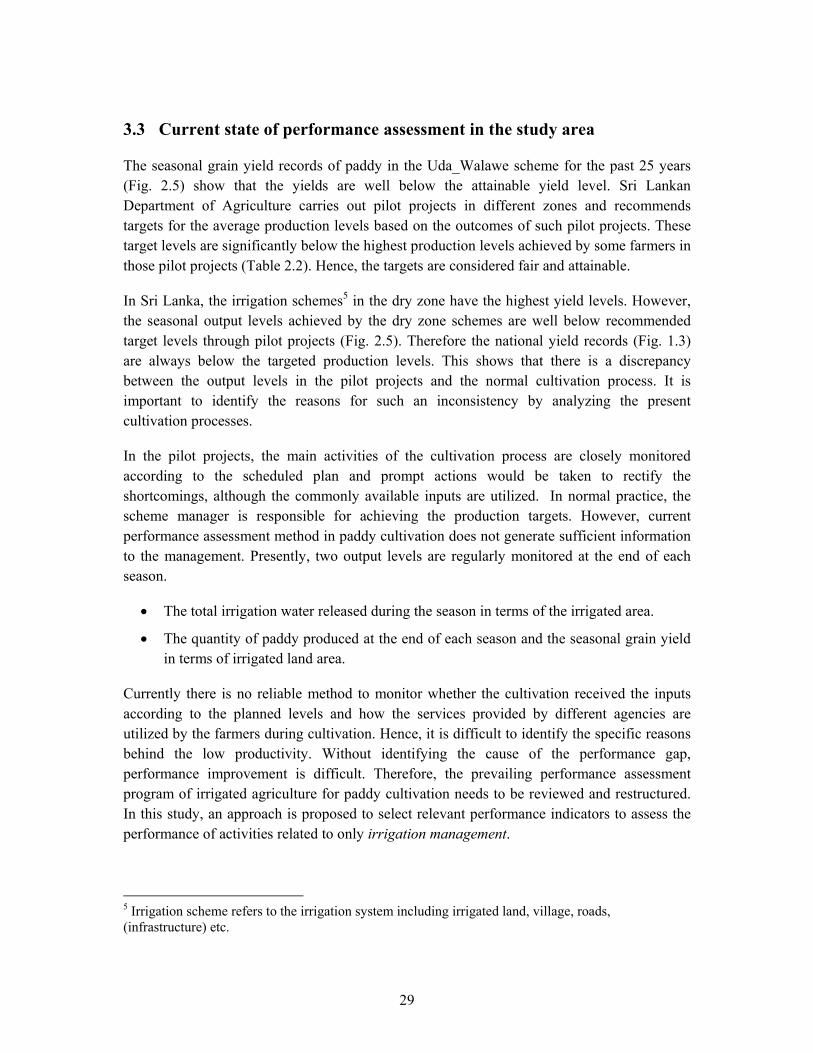
The seasonal grain yield records of paddy in the Uda_Walawe scheme for the past 25 years (Fig. 2.5) show that the yields are well below the attainable yield level. Sri Lankan Department of Agriculture carries out pilot projects in different zones and recommends targets for the average production levels based on the outcomes of such pilot projects. These target levels are significantly below the highest production levels achieved by some farmers in those pilot projects (Table 2.2). Hence, the targets are considered fair and attainable.

In Sri Lanka, the irrigation schemes5 in the dry zone have the highest yield levels. However, the seasonal output levels achieved by the dry zone schemes are well below recommended target levels through pilot projects (Fig. 2.5). Therefore the national yield records (Fig. 1.3) are always below the targeted production levels. This shows that there is a discrepancy between the output levels in the pilot projects and the normal cultivation process. It is important to identify the reasons for such an inconsistency by analyzing the present cultivation processes.

In the pilot projects, the main activities of the cultivation process are closely monitored according to the scheduled plan and prompt actions would be taken to rectify the shortcomings, although the commonly available inputs are utilized. In normal practice, the scheme manager is responsible for achieving the production targets. However, current performance assessment method in paddy cultivation does not generate sufficient information to the management. Presently, two output levels are regularly monitored at the end of each season.

• The total irrigation water released during the season in terms of the irrigated area.

• The quantity of paddy produced at the end of each season and the seasonal grain yield in terms of irrigated land area.

Currently there is no reliable method to monitor whether the cultivation received the inputs according to the planned levels and how the services provided by different agencies are utilized by the farmers during cultivation. Hence, it is difficult to identify the specific reasons behind the low productivity. Without identifying the cause of the performance gap, performance improvement is difficult. Therefore, the prevailing performance assessment program of irrigated agriculture for paddy cultivation needs to be reviewed and restructured. In this study, an approach is proposed to select relevant performance indicators to assess the performance of activities related to only irrigation management.

5 Irrigation scheme refers to the irrigation system including irrigated land, village, roads, (infrastructure) etc.

30

3.4 Major aspects related to irrigated agriculture

Irrigated agriculture can be described as a set of inter-related processes by which individual water users (or user organizations) and water institutions use water together with other input resources to grow crops (Fig. 3.2) in relation to their goals (Bos, 2001). The management activities, that control the level of inputs and the processes, determine crop yield. Performance assessment of irrigated agriculture can be related to the processes, level of outputs (e.g. crop production), and the efficiency of the outputs over inputs (e.g. grain yield in terms of cultivated area). Also, the degree of achieving ultimate goals using the optimum amount of resources determines how effectively the input resources have been utilized to produce the desired outputs i.e. effectiveness of the process.

Figure 3.2 Identification of major aspects of irrigated agriculture through analyzing its inputs, processes, and outputs.

Inflow control

Outflow control

Delivery control

Drainage control

Land management

Generaladministration

Systemmaintenance Cultivation

Rehabilitation

Infrastructure development

Water Balance

Environmental constraints

Socio-economic

Processes

Major aspects of irrigated agriculture

Input Resources[water, land, labor, machinery, and other inputs]

Operational level outputs

Strategic level outputs

Routine maintenance

Canal flow fluctuations

Crop water deficits

Drainage discharges

Downstream flooding

Water stagnation and down stream effects

Repairs to the system

Crop production

Return on investment

Productivity

Paddy price and farmer’s income

National economy

Inflow control

Outflow control

Delivery control

Drainage control

Land management

Generaladministration

Systemmaintenance Cultivation

Rehabilitation

Infrastructure development

Water Balance

Environmental constraints

Socio-economic

Processes

Major aspects of irrigated agriculture

Input Resources[water, land, labor, machinery, and other inputs]

Operational level outputs

Strategic level outputs

Routine maintenance

Canal flow fluctuations

Crop water deficits

Drainage discharges

Downstream flooding

Water stagnation and down stream effects

Repairs to the system

Crop production

Return on investment

Productivity

Paddy price and farmer’s income

National economy

31

3.5 Role of state water institutions in irrigated agriculture, Sri Lanka

Generally, water institutions deal with the water policy, water law, and water administration. The Department of Irrigation of Sri Lanka, has more than hundred years of experience, is responsible for preparing development proposals for water resources as well as implementing such proposals. In coordination with other line agencies, the Irrigation Department and the Mahaweli Authority of Sri Lanka manage all major irrigation schemes i.e. the irrigation schemes where the command area is greater than 400 ha. The Irrigation Department designs appropriate programs to improve performance of the schemes under its management and also implements such programs while providing irrigation facilities to the farmer community.

The only water law in the country is the Irrigation Ordinance (1946) as amended by the Irrigation Act in 1994. The Irrigation Ordinance stipulates conservation of water through following functions and activities in the irrigated agriculture.

• Powers entrusted to farmer organizations and their duties.

• Formation of Project Management Committees for major irrigation schemes and their duties.

• Constitution of district agriculture committees and their duties.

• Construction and maintenance of irrigation systems.

• Protection of irrigation systems and conservation of water.

To make rational decisions on crop cultivation, a project management committee is formed for each major irrigation scheme. This committee consists of farmer representatives and the representatives of all line agencies related to irrigated agriculture. In this committee, 50% of the total membership are farmers. The District Agriculture Committee (DAC) is the central administrative committee in a particular district to take district level decisions. The District Agriculture Committee is presided by the District Secretary and is composed of senior officials from other related organizations (Fig. 3.3).

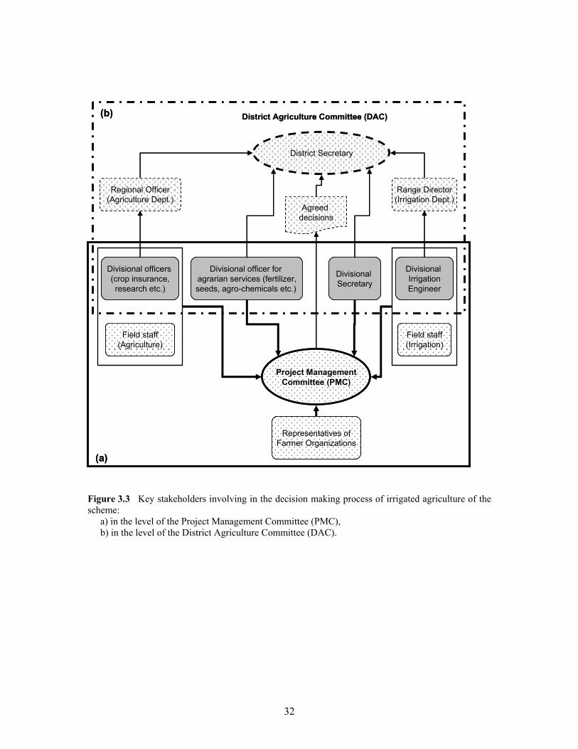
32

Figure 3.3 Key stakeholders involving in the decision making process of irrigated agriculture of the scheme:

a) in the level of the Project Management Committee (PMC), b) in the level of the District Agriculture Committee (DAC).

Project ManagementCommittee (PMC)

Divisional Secretary

Divisional IrrigationEngineer

Field staff(Irrigation)

Field staff(Agriculture)

Divisional officers (crop insurance,research etc.)

Divisional officer for agrarian services (fertilizer,seeds, agro-chemicals etc.)

Range Director(Irrigation Dept.)

District Secretary

Regional Officer(Agriculture Dept.)

Representatives ofFarmer Organizations

District Agriculture Committee (DAC)

Agreed decisions

(a)

(b)

Project ManagementCommittee (PMC)

Divisional Secretary

Divisional IrrigationEngineer

Field staff(Irrigation)

Field staff(Agriculture)

Divisional officers (crop insurance,research etc.)

Divisional officer for agrarian services (fertilizer,seeds, agro-chemicals etc.)

Range Director(Irrigation Dept.)

District Secretary

Regional Officer(Agriculture Dept.)

Representatives ofFarmer Organizations

District Agriculture Committee (DAC)

Agreed decisions

(a)

(b)

33

The Irrigation Ordinance describes the conditions on using irrigation water for agriculture, and is the prevailing water policy for irrigated agriculture. Water resources development plans for irrigated agriculture are prepared by the Irrigation Department. For domestic and industrial usage of water, National Water Supply and Drainage Board, another state organization furnishes respective proposals for the Government. At the feasibility stage, all such proposals are subject to the approval of the Irrigation Department. Thus, the Irrigation Department plays the coordinating role as the premier “water institution” for activities such as water resources development for irrigation, irrigation management, infrastructure development, capacity building, etc.

3.6 Key stakeholders and managerial hierarchy in irrigated agriculture

The paddy cultivating farmers have great expectations on improving their social life by increasing their income level. The Government intends to improve the social life of the farmer community. The Irrigation Department (i.e. the water institution for irrigation) coordinates and implements the national program of food security through provision of irrigation facilities to the farmer community while managing the irrigation schemes. In this context, the key stakeholders of irrigated agriculture are the Government, the Irrigation Department and the farmer organizations. Within the objectives of the process of irrigated agriculture, the interaction between each key stakeholder (Fig. 3.4) determines how they are accountable to each other in terms of its major aspects, which have already been defined. Sustainability of the entire process is the shared responsibility of all parties involved.

Figure 3.4 Interaction of key stakeholders for the sustainability of irrigated agriculture.

Socio-economic performance from

operationalto strategic

level

Socio-economic performance at

community level

Performance on water balance, and

environment

Sustainability of irrigatedagriculture

Government(National policy on food security

and social needs for farmer community)

Water institution(Irrigation Department)

Farmerorganizations

Socio-economic performance from

operationalto strategic

level

Socio-economic performance at

community level

Performance on water balance, and

environment

Sustainability of irrigatedagriculture

Government(National policy on food security

and social needs for farmer community)

Water institution(Irrigation Department)

Farmerorganizations

34

3.7 Boundary conditions for the performance assessment

To establish limits on the extent of the performance assessment, suitable boundaries should be defined. Firstly, the boundary conditions for the spatial distribution over the command area and for the time scale of data presentation need to be established. The significance of spatio-temporal changes over the system operations and the stakeholder requirements are considered.

Spatial boundaries of the irrigated agriculture sector depend on stakeholder requirements of the management hierarchy shown in Fig. 3.1:

• At the upper level, the spatial boundaries are established on the basis of district administration of the country.

• At the lower strategic levels i.e. ministry and line organization, the spatial boundaries are confined to each major irrigation scheme.

• Since the tactical managers perform the overall coordination of the schemes, specific spatial boundaries cannot be established.

• At the operational level of this study, based on the type of system administration of each scheme, the spatial boundaries are established for the four sub-schemes: the Left bank and the Right bank command areas of the Uda_Walawe scheme, and the Left bank and the Right bank command areas of the Liyangastota scheme. These boundaries are the spatial limits for the scheme managers. The performance assessment should start from each sub-scheme level. By reviewing the situational requirements and the nature of the problems encountered, performance assessment could be extended to the secondary or tertiary levels of the command area.

In associated with the time scale, the field data are acquired and processed on daily basis for the operational activities. In the seasonal cultivation plan, one common water delivery schedule is prepared for each sub-scheme i.e. within the sub-scheme, the starting date and the last date of water delivery, are fixed. Also, a uniform cultivation pattern is recommended i.e. similar crop varieties with the same growing period. However in practice, these schedules are subject to change with the changing of field conditions. For paddy cultivation, water deliveries are modified every 1 or 2 weeks. Hence, the temporal extent of the performance assessment could begin with 10 day intervals.

Given the broader perspective of irrigated agriculture in Sri Lanka, the purpose of assessing irrigation performance is not restricted to the individual farm level problems. The managers may have to attend to the problems of public (e.g. malaria breading caused by stagnant water) as well as of subordinating staff (e.g. resources constraints of field workers). Therefore, the boundaries are not always confined to system level operations. The internal and the external environment of the scheme may influence over the functioning of the irrigation scheme.

35

Considering the extents of such influences other boundaries should be defined, which are sometimes less clear and rather difficult to understand i.e. some physical limits on the external environment. However, they influence on the systems’ performance and consequently on the attainment of goals. The most common of such boundaries are socio-economic system, political system, physical system, and constraints on resources (Fig. 3.5). Since the irrigation schemes are managed by state sector service organizations (e.g. Irrigation and Agriculture departments) benefiting the nation and all the resources are valued by society.

Figure 3.5 Identification of boundary conditions in performance assessment.

Spatial extent

Temporal extent

Political system

Socio-economic

system

Physical system

Resourceconstraints

Water institutionsWater resources development for irrigationIrrigation management Infrastructure developmentCapacity building

Major aspects ofIrrigated agriculture Water balance and routing servicesSocio-economic and constraintsEmerging services

Spatial extent

Temporal extent

Political system

Socio-economic

system

Physical system

Resourceconstraints

Water institutionsWater resources development for irrigationIrrigation management Infrastructure developmentCapacity building

Major aspects ofIrrigated agriculture Water balance and routing servicesSocio-economic and constraintsEmerging services

36

3.8 Rationale of selecting performance indicators for the study area

The process of selecting appropriate indicators should focus on the intervention between each key stakeholder group, with respect to major aspects of irrigated agriculture. In this process three distinctive combinations are considered (Fig. 3.4):

• Interaction between the water institution and farmer organizations.

• Interaction between farmer organizations and the Government.

• Interaction between the water institution and the Government.

Out of the long list of performance indicators published in ICID guidelines (1978) and other literature (e.g. Levine, 1982; Makin et al., 1990; Wolters and Bos, 1990; Molden and Gates, 1990; Sharma et al., 1991; Molden and Sakthivadivel, 1999; Bastiaanssen and Bos, 1999), a minimum number is chosen, considering the cost of collection and data handling. Also, it is needed to verify whether these indicators are quantifiable from regular field measurements. Sometimes other measurements or techniques may be required. As such, the feasibility of doing so with the available facilities and resources needs to be determined. The application of satellite remote sensing and GIS is one such possibility. Further, it is necessary to check whether the parameters can be measured or collected with sufficient accuracy. Finally, the cost effectiveness should also be considered because the paddy cultivation is a heavily subsidized process. Fig. 3.6 depicts the applicability of these three conditions (i.e. feasibility of taking measurements, the accuracy of measurements and the cost effectiveness). The process of selecting most relevant performance indicators (step 1 of Fig. 3.6) is explained in next section. Each indicator listed in Table 3.1 was tested on the process described in Fig. 3.6. After passing the tests, it was added to Table 3.2.

In order to quantify performance indicators, canal flows of the Liyangastota schemes and reservoir releases of the Uda_Walawe scheme were available. These data were obtained from the respective scheme managers and the IWMI database for Ruhuna basin. Drainage data were started to collect by fixing new flow gauges since 2001. Cropping patterns and cultivation data were obtained from the offices of respective scheme managers. Rainfall data were collected from the IWMI database for Ruhuna basin. Other weather data (temperature, humidity, wind speed, daily durations of sunshine etc.) were obtained from the Meteorology Department, Sri Lanka. Cropping data were obtained from the publications of the Central Bank and the Department of Census and Statistics.

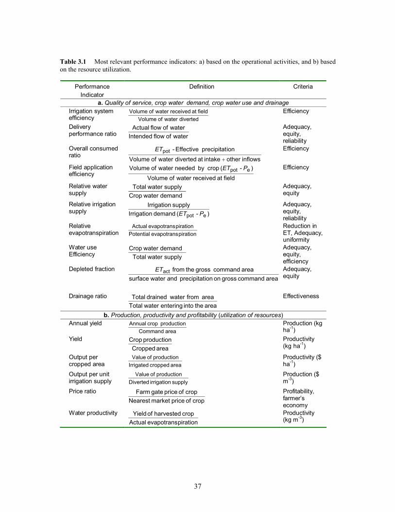
37

Table 3.1 Most relevant performance indicators: a) based on the operational activities, and b) based on the resource utilization.

Performance Indicator

Definition Criteria

a. Quality of service, crop water demand, crop water use and drainage Irrigation system efficiency diverted waterof Volume

field at received waterof Volume Efficiency

Delivery performance ratio waterofflow Intended

waterofflow Actual Adequacy, equity, reliability

Overall consumed ratio inflows other intake at diverted waterof Volume

ionprecipitat Effective -pot+

ET

Efficiency

Field application efficiency field at received waterof Volume

)- ( cropby needed waterof Volume epot PET

Efficiency

Relative water supply demand waterCrop

supply waterTotal Adequacy, equity

Relative irrigation supply )- ( demand Irrigation

supply Irrigation

epot PET Adequacy,

equity, reliability

Relative evapotranspiration pirationevapotrans Potential

pirationevapotrans Actual Reduction in ET, Adequacy, uniformity

Water use Efficiency supply waterTotal

demand waterCrop Adequacy, equity, efficiency

Depleted fraction area command gross on ionprecipitat nd watersurface

area command gross the from acta

ET

Adequacy, equity

Drainage ratio area the into entering waterTotal

area from waterdrained Total Effectiveness

b. Production, productivity and profitability (utilization of resources) Annual yield

area Commandproduction crop Annual Production (kg

ha-1) Yield

area Croppedproduction Crop

Productivity (kg ha-1)

Output per cropped area area cropped Irrigated

production of Value Productivity ($ ha-1)

Output per unit irrigation supply supply irrigation Diverted

production of Value Production ($ m-3)

Price ratio crop of price market Nearest

crop of price gate Farm Profitability, farmer’s economy

Water productivity pirationevapotrans Actual

crop harvested of Yield Productivity (kg m-3)

38

Figure 3.6 Process of selecting performance indicators: 1) selecting most relevant indicators from the published long lists, and 2) assessing practicality of the selected indicators for the local conditions.

Areparameters quantifiable

from regular fieldmeasurements?

Is arrangingnew field

measurementsfeasible?

Isquantifying the

parameter cost effective?

Is arranging new technology

feasible?

Yes

YesYes

Yes

YesNo

No

No

Canparameter

be measured/collected with sufficient

Accuracy?

No

Accepted indicator for performance assessment

program

Review selected performance Indicators

No

• Common objectives between each stakeholder groups.

• Concerns of each stakeholder groups on their activities related to irrigated agriculture.

Long-list of performance indicators

described in international literature

Select most relevant performance indicators

Step 1

Step 2

Areparameters quantifiable

from regular fieldmeasurements?

Is arrangingnew field

measurementsfeasible?

Isquantifying the

parameter cost effective?

Is arranging new technology

feasible?

Yes

YesYes

Yes

YesNo

No

No

Canparameter

be measured/collected with sufficient

Accuracy?

No

Accepted indicator for performance assessment

program

Review selected performance Indicators

No

• Common objectives between each stakeholder groups.

• Concerns of each stakeholder groups on their activities related to irrigated agriculture.

Long-list of performance indicators

described in international literature

Select most relevant performance indicators

Step 1

Step 2

39

3.9 Discussion on selected performance indicators

The interaction between the water institution and farmer organizations relates to the aspects of water balance and environment. A service agreement between the water institution and farmer organization describes the functions of each party related to the common targets. In Sri Lanka, the service agreement contains some conditionally agreed decisions made at the project management committee (PMC) through a negotiated process. The agreed conditions and decisions are documented and submitted to the District Agriculture Committee (DAC). Prior to the start of forthcoming cultivation season, the document is discussed and approved with necessary amendments. Generally this document contains the following terms and conditions.

• The rationale of water delivery considering the water availability and expected supply of water to the system.

• The time schedule of cultivation including routine maintenance, land preparation, cultivation, and harvesting.

• Cropping pattern (type and variety) for each irrigation scheme.

• Responsibilities of farmer organizations and the water institution on the operation, maintenance of the system, and other related issues.

The water institution, together with farmer organizations, formulates the cropping calendar of the cultivation season by fixing a common schedule for each irrigation sub-scheme of the study area. Related to the cropping calendar, the concerns and the objectives of the two stakeholder groups are considered. The activities related to the cropping calendar influence the operational performance. However, the trends of outcomes at operational level are used to assess the strategic performance.

While implementing the common cultivation schedule for each sub-scheme, the water institution needs to maintain the uniformity and equity of water delivery over the command area. Hence, one should select performance indicators that ensure the quality of service rendered by the water institution through water delivery (Table 3.1a).

From the farmer’s point of view, water adequacy for crop growth i.e. crop water demand, is more important. In practice, the inconsistency between water supply and the demand causes changes in actual water consumption by the crops. The water manager needs to know the zones where the water consumption is below target levels, which can be monitored through an indicator that measures the relative evapotranspiration (Table 3.1a).

Because paddy cultivation is a high water using process, a substantial quantity of irrigation water flows through the drainage canals, which is re-used by the downstream users. In

40

addition, excess, or short supply of water, due to poor operational control, an upstream canal breach or high rainfall intensity may cause unusual flow rates in drainage canals. Thus, measurement of excess quantity of drainage water helps in assessing the water balance in the command area and it can be used as a warning for under-performance (Table 3.1a).

The interaction between the Government and farmer organizations focuses on economic and social needs. The subsidy level on agro-based imports (e.g. fertilizer and agro-chemicals, machinery and equipment), credit facilities for farming activities on low interest rates, crop insurance schemes, and fixing farm-gate price over paddy are the socio-economic supports extended to the farmer community (profitability). To achieve the goal of self sufficiency, increased production of paddy during the season is desired by the Government. Thus, it is necessary to assess the changes in crop production per unit area (productivity) and also the changes in market conditions for paddy crop (Table 3.1b).

The intervention between the government and the water institution focuses on economic performance from the operational level to the strategic level. At the bottom level of the management hierarchy, performances are assessed per sub-scheme (primary) level over 10 day intervals i.e. moderate spatio-temporal scale, compared to the daily observations with tertiary or secondary levels of the command area. At the middle management level the temporal scale of the information is set in broader time spans (e.g. monthly, growing stages, seasonally) whereas the spatial scale is confined to the scheme level and above (e.g. scheme, district, river basin, national). At higher management levels, the performance assessment information is required on rather generalized spatio-temporal scales only. Political management is interested in the utilization of resources (i.e. land and water) over the process of food production. For this, performance indicators to assess the change in grain yield in terms of the land area irrigated as well as per unit amount of water supplied or used by the crop for producing grain (Table 3.1b). In addition, the performance indicators selected under other scenarios can be used at this stage, with suitable spatio-temporal scales i.e. spatial and time integration of indicators listed in Table 3.1.

By considering the objectives of the study and the purpose of the performance assessment, a minimum number of indicators were accepted from the selected list (Table 3.2).

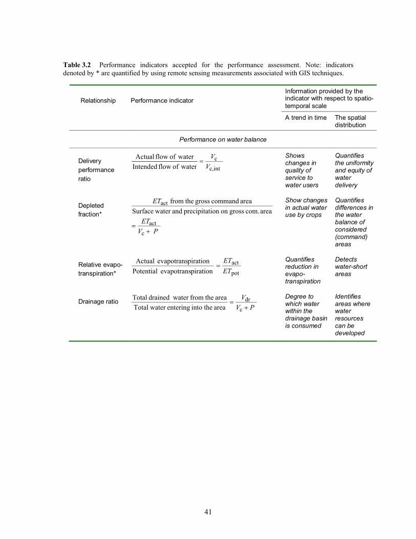
41

Table 3.2 Performance indicators accepted for the performance assessment. Note: indicators denoted by * are quantified by using remote sensing measurements associated with GIS techniques.

Information provided by the indicator with respect to spatio-temporal scale

Relationship

Performance indicator

A trend in time The spatial distribution

Performance on water balance

Delivery performance ratio

waterofflow Intended waterof flow Actual

c,int

cV

V=

Shows changes in quality of service to water users

Quantifies the uniformity and equity of water delivery

Depleted fraction* area com. grosson ion precipitat and water Surface

area command gross thefrom actET

PVET

+=

c

act

Show changes in actual water use by crops

Quantifies differences in the water balance of considered (command) areas

Relative evapo-transpiration* pirationevapotrans Potential

pirationevapotrans Actual

pot

actETET

= Quantifies reduction in evapo-transpiration

Detects water-short areas

Drainage ratio area theinto entering water Totalarea thefrom water drained Total

PVV

c

dr+

= Degree to which water within the drainage basin is consumed

Identifies areas where water resources can be developed

42

Table 3.2 continued.

Information provided by the indicator with respect to spatio-temporal scale

Relationship

Performance indicator

A trend in time

The spatial distribution

Socio-economics performance

Yield Yact * area Cropped

production Crop crop

grainAm

= Quantifies change in crop yield or value per unit area

Shows spatial variation in productivity (kg/ha)

Water productivity WPm,ET *

pirationevapotrans Actualcrop harvested of Yield

grain

actETm

= Quantifies change in crop yield or value per m3 water supplied

Shows spatial variation in productivity (kg/m3)

Price ratio Rprice crop of pricemarket Nearest

crop of price gate Farm price

priceMF

= Shows changes in marketing conditions for irrigated crop(s)

Shows areas where farmers may have to stop irrigation

43

4. Satellite remote sensing approach to determine crop parameters

4.1 Introduction

In the performance assessment of irrigated crops, satellite remote sensing techniques can be applied to quantify spatial-temporal variations of water use in two broad areas.

• Classification of land cover (e.g. water bodies, bare soils, and vegetation) and agricultural land use (irrigated and non irrigated areas).

• Estimating variations of important crop parameters such as evapotranspiration, root zone soil moisture and plant growth.

Land use, classification using satellite data becomes useful in situations where detailed digitized ground maps are not available, and especially when they are not updated regularly through overland surveys. The situation in the two Sri Lankan irrigation schemes which forms the study area of this thesis is just that, and spectral properties of satellite images of sufficient resolution are used to demarcate the areas under paddy cultivation.

Estimating crop parameters with satellite spectral data has the advantage that accessing such information being easy, fast and economical. However it faces a difficulty because algorithms used to interpret such data require too much input data which beats the purpose of applying remote sensing. For the particular case involved in this study, namely, determining the requirement of evaporative depletion of water at different stages of crop growth and the seasonal grain yield of paddy in irrigation schemes of Sri Lanka, a simplified algorithm called SEBAL (Surface Energy Balance Algorithm for Land) was used (Bastiaanssen, 1995). It overcomes such constraints by using the concept of evaporative fraction (i.e. latent heat, as a fraction of net available energy per given area) and the surface energy balance (Ahmad, 2002) which require a minimum amount of climatic data as inputs, generally available from the Meteorology Department of Sri Lanka.

4.2 Satellite measurements

MODIS measurements have been used as the remote sensing inputs in the study. Out of 36 MODIS spectral bands of different spatial resolutions, 4 have been used for the SEBAL model. The spatial resolution of both visible (band 1) and near infrared (band 2) bands is 250 m at satellite nadir and for both thermal bands (band 31 and 32) spatial resolution is 1000 m. However, the ultimate results are confined to the 1000 m resolution. Therefore the images of band 1 and band 2, which were pre-processed into the standard spatial resolution of 1000 m, are used for image analyses.

44

Furthermore, the resolution tends to vary with the view angle, i.e. the vertical angle from the satellite nadir towards the image area. Thus, images with view angles greater than 50 are discarded. Since cloudy images also have to be discarded, out of daily images of MODIS, only 40-60 % per month are effective for the SEBAL analysis.

Hence, it is necessary to assure whether such a moderate number of images are sufficient for the study. In Sri Lanka, for irrigated paddy cultivation, water is delivered under gravity and most of the distribution and field canals are unlined. The wetting conditions for paddy lands are staggered in 1 to 2 weeks intervals. Yet, since the output information is not required on daily basis MODIS images could be satisfactorily used for this study.

4.3 Classification approach

For either of the two irrigation schemes under study, updated digital project maps are not available, neither have field surveys done to update land use boundaries. Carrying out a land survey is a costly and time consuming activity. Therefore, it was decided to use satellite spectral classification techniques to demarcate the irrigation command areas.

Each 1000 m × 1000 m square MODIS pixel covers an area of 100 ha over the ground, and but these pixels cannot fit the smaller scale irregular periphery of the command area (Fig. 4.1). Therefore in pixel based classification using low spatial resolution images such as the MODIS, it is quite difficult to differentiate the irregular shaped objectives. In addition, if there is any pixel adjoining the boundary, which is having almost similar spectral properties, may be wrongly classified as one belongs to the area concerned.

45

Figure 4.1 A part of the study area overlaid on a pixel grid similar to the MODIS pixel size, showing irregularity of the land cover and the effect of boundary pixels: a) a part of the study area as a sample, b) sample area overlaid by a pixel grid of the MODIS pixel size, and c) spatial extent of the sample area represented by the pixel grid similar to the MODIS pixel size.

However in large irrigation schemes in the dry zone of Sri Lanka, paddy cultivated areas could be clearly distinguished using near infra-red spectral bands due to its high chlorophyll content i.e. spectral properties of the land cover. Similarly, if the classification is carried out during the off-season, the command area could be classified as bare soils using mid infra-red bands. If there is any wrong classification encountered in the demarcation of the periphery along the command area using low spatial resolution images, the error would be considerably high. Thus, the precision and the accuracy of the boundary classification along an irregular periphery depend on the pixel resolution as well as the spectral properties of the existing land cover. Therefore, in order to obtain a smooth precise boundary of the command area, a cloud-free 30 m × 30 m resolution Landsat-7 ETM+ image was used for land use classification.

The most common such techniques using false colour composites are supervised, unsupervised, hybrid and digital classification. To classify the command area, the spectral false color composite technique by changing the band combination was applied. In this method, the command area could be clearly identified, but some locations along the lower part of boundary were not clearly classified over the color composite map. Through a physical observation along such locations, it was found that the land cover out side the boundary was a kind of vegetation grown in marshy lands. This vegetation cover shows similar spectral characteristics as rice. GPS survey techniques and digital topographical maps of 1: 50000 scale were used to demarcate the such boundaries. Finally, a vector based digital boundary map was prepared for the study area displaying the command areas of both schemes (Fig. 4.2).

b ca

MODIS pixels fitting over the sample area

Sample area

b ca b ca

MODIS pixels fitting over the sample area

Sample area

46

Figure 4.2 Boundary map prepared to identify each command area of the Uda_Walawe scheme and the Liyangastota scheme using a color composite map of the Landsat 7 ETM+ image associated with GIS techniques.

Uda_Walawe right bank command area

Liyangastota left bank command area

Liyangastota right bank command area

Uda_Walawe left bank command area

km4 0 4 8

N









km4 0 4 8

N

47

4.4 SEBAL approach

SEBAL can analyze the water productivity at the irrigation system level as well as at the basin level in Sri Lanka (e.g. Bandara, 2003; Bastiaanssen and Bandara, 2001; Bastiaanssen and Chandrapala, 2003). A number of publications have been released on SEBAL approach and its’ applications describing the entire procedure (Bastiaanssen, 1995; Bastiaanssen, 2000; Bastiaanssen et al., 2003). However, two critical issues encountered in the SEBAL application of this study are discussed: 1) the time scale of SEBAL outcomes, and 2) assimilation of radiometric surface temperature into aerodynamic temperature.

The instantaneous latent heat flux )m(W -2λET , which is associated with the actual evapotranspiration, is calculated for each pixel of the image as a ‘residual’ of the surface energy balance equation:

HGRET - 0n −=λ )m(W -2 4.1

where nR is the net radiation flux (actual energy available at the surface), 0G is the soil heat flux, and H is the sensible heat flux to the air.

Eq. 4.1 can be re-written and expressed as latent heat flux by considering evaporative fraction (-) Λ and net available energy )( 0n GR − :

)( 0n GRΛET −=λ 4.2

where

HλETλET

GRλETΛ

+=

−=

0n 4.3

Time scale of SEBAL outcomes: The net available energy in Eq. 4.2 may have different time scales, i.e. from instantaneous (at the time of the satellite overpass) to daily-integrated values, or for periods elapsing between two consecutive satellite images. Depending on the time scale chosen, different time integrations of )( 0n GR − should be obtained. For the time scale of 1 day or multiple days, 0G can be ignored. Thereby net available energy 0n GR − reduces to net radiation nR . Following Shuttleworth et al. (1989), the instantaneous evaporative fraction is considered similar to its daily counterpart (Brutsaert and Sugita, 1992; Crago, 1996), and is used to compute the actual 24-hour evaporation from the instantaneous latent heat fluxes. For the daily time scale, ) d (mm -1

24ET is formulated as:

n24w

324

1086400 ΛRλρ

ET ×=

4.4

48

where n24R is the 24-hour average net radiation, )kg (J -1λ is the latent heat of the

vaporization and )m (kg -3wρ is the density of water. Eq. 4.2 requires Λ , nR and 0G to be

known.

Farah (2001) found that the accumulated evapotranspiration for a period of 10 to 20 days can be predicted satisfactorily from the following time integrated equation:

t,t ΛRρλ

ET dn24w

3d

1086400×=

4.5

where )interval (mm 1-dtET is the actual evapotranspiration during interval td measured in

days and )m(W -2dn24 t,R is the average n24R value for the time interval td . Farah (2001)

recommends that Eq. 4.5 computes the time integration of evapotranspiration for a period of 10 - 20 days. The computation of 24ET for a particular day within that period using Λ as a constant value estimated from the satellite overpass is however not accurate. It can be deduced that computing 24ET for days with no satellite measurements is erroneous. The time integrated values of tETd for a period of 10 days (i.e. by lowering the upper limit of Eq. 4.5 from 20 days to the maximum of 10 days) can be however predicted at a sufficient accuracy even with a temporally constant value of Λ .

In order to compute daily values or integrated daily values of evapotranspiration, n24R requires to be known. The conversion of global radiation into net radiation for time scale

of days was achieved using a simplified formula (Bruin and Stricker, 2000):

↓

↓↓ −−=

exo0n24 110)(

K

KKrR 1 4.6

where )(0 −r is the surface albedo, )m(W 2-↓K is the global radiation at the surface level, and

)m(W -2exo↓K is the theoretical extra-terrestrial solar radiation. Incoming solar radiation was

computed using the standard conversion equation suggested by Allen et al. (1998):

↓↓

+= exo0.50.25 K

NnK 4.7

where n (hr d-1) is the day-duration of actual sunshine measured in the field and N (hr d-1) is the theoretical maximum day-duration of sunshine.

49

Assimilation of radiometric surface temperature into aerodynamic temperature: Thermal infrared remotely sensed surface temperature (i.e. radiometric surface temperature T0) has been widely used in operational models to evaluate the spatial distribution of the energy balance components. However, the performance of the approach has been under question since radiometric surface temperature T0 cannot be assimilated into aerodynamic surface temperature. Under dense canopy, the difference between two temperature values is very small, which leads to small errors in heat flux prediction. Over sparsely vegetated surfaces, however, the difference can exceed 100 C and then it can be largely overestimated (Chehbouni et al., 1997). The SEBAL has overcome the difficulty of relating radiometric temperature 0T to source height ohz (Bastiaanssen, 2000). The procedure presumes that there is no H from the wet pixel and there is no evaporation λET from the dry pixel. SEBAL first computes H at extreme dry (hottest) and wet (coldest) locations because H is not known for all other pixels. This eliminates the need to install expensive instruments to determine H. Thus, a linear relationship between the temperature difference and the surface temperature (T0) is developed to describe the spatial distribution of the temperature difference which is a function of H.

Basically, a dry place is considered as drier than any other location with similar conditions but has a low temperature. However, this is not always true because land uses are not uniform within the image. Identification of dry pixels is based on the thermal infrared channel. Having selected a group of pixels with the highest range of surface temperature, the locations of dry pixels are manually identified on the satellite image using the knowledge of land use. In this study, the sandy areas close to the coastal belt were selected as dry pixels. As for wet pixels, it was however not appropriate to select wet locations like irrigation reservoirs. Morse et al. (2000) recommended to avoid deep water bodies due to the problem of lag in stored heat flux

0G into the body that may not be available at the same instant as nR , H and λET . Therefore marshy lands in wetland areas were selected as wet locations. However, selection of wet and dry pixels in the SEBAL model is a rather subjective as well as a knowledge based exercise.

50

4.5 Estimation of potential evapotranspiration

The potential evapotranspiration rate )d (mm -1potET is estimated from the Penman-Monteith

equation (Monteith, 1965; Rijtema, 1965; Smith, 1992; Allen et al., 1998):

++

−+

×=

ha,

minc,air

ha,

actsatairair0nv

w

3pot

1γ

)-(

1086400

rr

∆

reecρGR∆

ρλET

v

(mm d-1)

4.8

where v∆ represents the slope of the saturated vapor pressure temperature relationship

)K (kPa -1 , nR is the net radiation flux density above the canopy )m(W -2 , 0G is the soil heat

flux density )m(W -2 , airρ is the mean air density at constant pressure )m (kg -3 , airc is the

heat capacity of moist air per unit mass )K kg (J -1-1 , sate is the saturated vapor pressure

(kPa) , acte is the actual vapour pressure (kPa) , λ is the latent heat vaporization )kg (J -1 , wρ

is the density of water )m (kg -3 , airγ is the psychrometric constant )K (kPa -1 , minc,r is the

minimum value of the surface resistance of canopy (i.e. when soil water is not limited, the canopy resistance cr reaches a minimum value minc,r ) )m (s -1 , and ha,r is the aerodynamic

resistance for heat transport )m (s -1 . In order to solve Eq. 4.8, daily weather data of air humidity, wind speed and air temperature are required.

The transfer of heat and water vapour from the evaporating surface into the air above the canopy is determined by the aerodynamic resistance ha,r . In most practical applications, the aerodynamic resistance ha,r is calculated as a function of crop height (m) ch and wind speed

)s (m -1zu (e.g. Allen et al., 1990, 1996, 1998; Brutsaert, 1982; D’Urso, 2001):

z

c

c

c

cu

z2

ohom

u

ha, 0.168 0.0123

0.667ln

0.1230.667

ln

lnln TT

uh

hzh

hz

uk

zdz

zdz

r

−×

−

=

−×

−

=

4.9

where uz and Tz are the measurement heights for wind speed and temperature, d is the zero-plane displacement height and the variables omz , ohz represent the roughness lengths for momentum and heat respectively being estimated from ch .The standard value for von Karman’s constant k is taken as 0.41 (-). Consequently, the aerodynamic resistance ha,r becomes a function of crop height and wind speed. The ch values for the dry zone paddy,

51

obtained from the Rice Research and Development Institute of Sri Lanka were used in this study (Fig. 4.3)

The surface resistance of the canopy cr describes the resistance of vapour flow through the transpiring crop and evaporating soil surface. Where the vegetation does not completely cover the soil, the resistance factor should indeed include the effects of evaporation from the soil surface. If the crop is not transpiring at a potential rate, the resistance depends also on the water status of the vegetation.

Potential evapotranspiration of a crop can be expected when there is no restriction due to either biological control or to soil water content. In practice, this situation is described as a well-watered condition of a crop.

An acceptable approximation to a much more complex relation of the canopy resistance for densely growing vegetation is generally computed as (Allen et al., 1996, 1998):

eff

leafc

LAIr

r = 4.10

where leafr is the canopy (stomatal) resistance of the vegetation per unit LAI and effLAI is the effective leaf area index contributing to evapotranspiration. For well watered agricultural crops (i.e. when soil water is not limited), when calculations are made on 24-hr basis the value of leafr is taken as 100 s m-1 (Monteith, 1965; Allen et al., 1989, 1990).

Figure 4.3 The height variation of a paddy crop (BG 358) grown in the dry zone of Sri Lanka under normal condition. Source: Rice Research and Development Institute of Sri Lanka (2005).

0

0.2

0.4

0.6

0.8

1

1.2

0 10 20 30 40 50 60 70 80 90 100

Growing period (d)

Cro

p he

ight

(m)

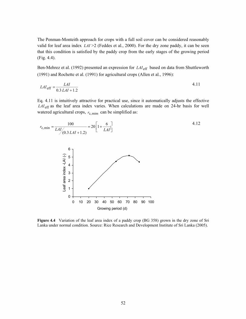
52

The Penman-Monteith approach for crops with a full soil cover can be considered reasonably valid for leaf area index LAI >2 (Feddes et al., 2000). For the dry zone paddy, it can be seen that this condition is satisfied by the paddy crop from the early stages of the growing period (Fig. 4.4).

Ben-Mehrez et al. (1992) presented an expression for effLAI based on data from Shuttleworth (1991) and Rochette et al. (1991) for agricultural crops (Allen et al., 1996):

1.2 0.3 eff +

=LAILAILAI 4.11

Eq. 4.11 is intuitively attractive for practical use, since it automatically adjusts the effective effLAI as the leaf area index varies. When calculations are made on 24-hr basis for well

watered agricultural crops, mimc,r can be simplified as:

+=

+=

LAILAILAI

r 61 20 1.2) (0.3

100 minc, 4.12

Figure 4.4 Variation of the leaf area index of a paddy crop (BG 358) grown in the dry zone of Sri Lanka under normal condition. Source: Rice Research and Development Institute of Sri Lanka (2005).

0

1

2

3

4

5

6

0 10 20 30 40 50 60 70 80 90 100

Growing period (d)

Leaf

are

a in

dex

-LA

I (-)

53

4.6 Estimation of biomass growth and grain yield

In Sri Lanka, rice yield is a key element for the dry zone development and is an indicator for national food security. Timely estimation of seasonal grain yield of paddy is essential to assess the level of self sufficiency in advance, and to take remedial measures (e.g. to import a deficit or to export a surplus), if necessary. A remote sensing model relating reflectance data to paddy crop parameters would be useful for monitoring of biomass and prediction of grain yield in time.

The Food and Agricultural Organization of the United Nations has developed several procedures to compute regional crop yields from the normalized difference vegetation index NDVI (-) using low resolution and high frequency satellite images (e.g. Hielkema, 1990). The visible and near infrared data of a satellite images can be used to form a “greenness index” or Normalized Difference Vegetation Index:

channeVisible channel infraredNear channel Visible - channel infraredNear

+=NDVI 4.13

And one commonly applied procedure is the development of empirical relationships between NDVI and crop yield. The general drawback of most methods using statistical relationships between NDVI and crop yield is that they have a strong empirical character and also the correlation coefficients yields from moderate to low (e.g. Gorten, 1993; Sharma et al., 1993). Moreover, crop yields basically depend on many more factors than chlorophyll presence (Rosema et al., 1998). For rice crop, the studies carried out by Gilabert and Melia (1990), Patel et al. (1985), and Casanova et al. (1998) have shown viable relationships between spectral response of paddy crop and its biomass.

Monteith (1972) pioneered the concept of calculating net primary biomass production as a function of Absorbed Photosynthetically Active Radiation (APAR). Experimental results have validated this concept for a number of crop types (e.g. Kumar and Monteith, 1981; Steven et al., 1983; Green et al., 1985; Wiegand et al., 1989, 1991; Casanova et al., 1998).

54

To determine the accumulation of biomass Bastiaanssen and Ali (2003) have given the following relationships (Eqs. 4.14 – 4.17):

∑

= ↓ tfKε t 0.48 PAR,24actB 4.14

where Bact (kg m-2) is the accumulated above ground dry biomass in period t, ε (g MJ-1) is the light use efficiency, t describes the period over which accumulation takes place, PARf is the fraction of photosynthetically active radiation absorbed by green leaves in a canopy, and the light use efficiency ε is expressed as:

Λ TTε 21ε′= 4.15

where ε’ is a maximum conversion factor for above ground biomass. When environmental conditions are optimal, T1 and T2 can be expressed as:

2optopt1 0.0005 0.02 0.8 TTT −+= 4.16

)}10 exp{0.3(-

)10 exp(0.2 monoptmonopt2 TTTT

T+−+

×−−+

=1

11

1

4.17

where Topt (0C) is the mean air temperature during the month of maximum leaf area index or NDVI development and Tmon (0C) is the mean monthly air temperature. The factor T1 essentially accounts for the reducing effect cooler regions have on the crop growth. Hence, for Sri Lanka as a tropical region, T1 can be taken as 1. T2 reduces the light use efficiency if the environmental temperature starts deviating from the optimum temperature and this is relevant for arid and semi-arid zones.

The conversion factor ε’ ranges 1.8 to 2.7 g MJ-1 (Bastiaanssen and Ali, 2003) for the rice varieties tested from 1989 to 1998. Therefore the average of above range 2.25 g MJ-1 has been used in this study.

The fraction PARf of photosynthetically active radiation absorbed by green leaves in a

canopy has been derived by both empirical (e.g. Daughtry et al., 1983; Steinmetz et al., 1990; Landsberg and Gower, 1997) and theoretical studies (Kumar and Monteith, 1981; Myneni et al., 1995). Remote sensing yields the opportunity to estimate PARf directly as a linear

function of NDVI (e.g. Hatfield et al., 1984; Asrar et al., 1992). Bastiaanssen and Ali (2003) have used the following linear relationship for rice by incorporating the experimental results from corn and soybeans (Daughtry et al., 1992), sunflower (Joel et al., 1997), and cereals (Myneni et al., 1997) and the same relationship is applied in this study:

NDVIf 1.257 0.161PAR +−= 4.18

55

Generating maps of PARf at the regional scale using NDVI is much more possible, since

NDVI can be calculated from multi-spectral sensors of most of the satellites.

Grain yield Yact is a component of the accumulated above ground dry biomass. Hence to predict paddy production, the accumulated biomass during the season should be multiplied by a harvest index hind (Horie et al., 1992). Richards and Townley-Smith (1987) has given a relationship to estimate the grain yield Yact as:

)m kg ( -1

2-

oi

indact m

hY actB

= 4.19

where moi (-) is the moisture content of the produce during the harvest.

The Rice Research and Development Institute in Sri Lanka (RRDI, 2005) indicates that the moisture content of paddy grain when the crop comes to the harvesting stage is almost 22%. For the storage of paddy grain, the recommended moisture content is 12% - 13%. To determine the seasonal harvest, sample measurements (i.e. weight of paddy grain) are taken at the end of the harvest; but before the storage. At this stage the moisture content remains slightly above the recommended level, thus, moi = 0.15 is taken for this study.

Through a research under open field condition, Janendra et al. (2004) mention a hind as 0.45 for medium duration rice in Sri Lanka (i.e. recommended rice in the dry zone). Hence, in computation of harvest, the hind = 0.45 is used.

57

5. Estimating actual evapotranspiration using remote sensing images with different spatial resolutions

5.1 Introduction

In order to monitor ETact in close intervals, ETact has been estimated using the MODIS measurements of 1000 m spatial resolution with daily images as explained in section 1.5 i.e. the higher the temporal resolution, the lower the spatial resolution. Therefore, it is necessary to assess whether the results are sufficiently accurate to support the management decisions of irrigation practices. Thus, ETact derived from the MODIS data are compared with satellite measurements having highest possible spatial resolution. Since the availability of the thermal band is an essential requirement for the SEBAL approach adopted for estimating ETact, either the Landsat ETM+ measurements or the ASTER measurements (Table 1.3) could be selected for the comparison. Due to the boundary problem of the ASTER images as explained in section 1.5, the Landsat ETM+ measurements were selected.

ETact depends on the land cover, land use and weather conditions. Hence, such a comparison would be realistic, if satellite data of different spatial resolutions were selected from one particular date. This was rather difficult task to match two satellite images with different properties such as temporal resolution, cloudiness, scan angle etc. (as explained in Table 1.3 and section 1.5). Having compared available Landsat-7 ETM+ images with suitable MODIS images, two satellite data sets, one from the MODIS and the other from the Landsat-7 ETM+, both acquired 14th March 2001 were selected for the comparison.

Thus, the Landsat-7 ETM+ images of 30 m spatial resolution are considered as the smallest possible pixel size which can be used for the comparison. This assumption is regarded to be valid until more precise satellite measurements become available which could have the facility of solving the surface energy balance. Thus, the error of ETact due to the spatial scale is described as the deviation of the resulting value of the energy balance (i.e. ETact) derived from the MODIS measurements with respect to that derived from the Landsat Measurements.

5.2 Constitution of errors due to pixel aggregation of spectral data

Since the input parameters of the MODIS and the Landsat measurements represent two distinctive pixel sizes, comparison between these output values which has the same disparity is unrealistic (Fig. 5.1). The study area is selected as the sample area to proceed with the SEBAL process using both data sets.

58

Figure 5.1 Comparison of one pixel of a MODIS image with Landsat pixels.

It is more practical to expand the smaller pixels of Landsat into the size of the larger pixel of MODIS by incorporating the neighbouring pixels. The geo-informatic software, Integrated Land and Water Information System (ILWIS), provides the facility to transform 30 m Landsat pixels into 1000 m sized pixels by linear aggregation of 33 pixels along each row and each column of the image: i.e. 30 m × 33 = 990 m ≈ 1000 m. However, such linear aggregation can constitute errors in two ways.

1) Some of the model functions of the SEBAL approach (e.g. NDVI ) are formulated by non-linear relationships among input variables. While computing ETact through the SEBAL approach, the linear aggregation of output parameters which have been derived through non-linear relationships can introduce errors.

2) In this study, the satellite measurements represent the spectral properties of the vegetation cover of the command area. Although the entire study area is mainly covered by paddy, in some areas cultivation is delayed because of water distribution problems. In addition, highlands within the command area are occupied by the framers to build their houses and with that the land is used as home gardens to cultivate coconut, banana, vegetable etc. In such areas spectral properties may be varying due to the heterogeneity of vegetation cover. Therefore, a normal distribution of spectral

One MODIS pixel of 1000 m × 1000 m

The MODIS pixel is replaced by 30 m ×30m Landsat pixels

Liyangastota left bank command area from a MODIS image

One MODIS pixel of 1000 m × 1000 m

The MODIS pixel is replaced by 30 m ×30m Landsat pixels

Liyangastota left bank command area from a MODIS image

59

measurement values cannot be assumed for each sample population, i.e. 33 × 33 set of pixels being used for the aggregation.

Since the spectral distribution in each 33 × 33 pixel set is not necessarily to be normal, the sample representative values (i.e. central tendency of the distribution) of the parameter ETact, have alternatively been computed by three different ways. The ILWIS software provides the facility to determine the central tendency of sample distribution by the following different ways.

• Pixel aggregation by taking the mean value of the sample distribution:

n

x

M

n

ii

i

∑== 1

5.1

where Mi is the aggregated spectral value of each simulated 1000 m pixel, xi is the value of each pixel inside the 33 × 33 set, and n is the number of pixels inside each set (n = 33 × 33 = 1089).

• Pixel aggregation by taking the median value of the sample distribution.

The median is defined as the middle value of a distribution. When pixel values are arranged in the ascending order, half the values are above the median and half are below the median. The median is less sensitive to extreme values of a distribution than the mean and this makes it a better measure than the mean for highly skewed distributions.

• Pixel aggregation by taking the mode value of the sample distribution.

By definition, mode is the most frequently occurring value in a distribution. The mode is greatly subject to sample fluctuations and there may be more than one mode values in a distribution. However, mode is the only measure of central tendency that can be used with nominal data.

The error due to non-linearity of the SEBAL model functions and the heterogeneity of the land cover cannot be differentiated while performing the computations. The error caused by non-linearity is illustrated in Fig. 5.2 using two different approaches of deriving SEBAL output.

60

Figure 5.2 Aggregation of spatially distributed values, following two different approaches: a) the linear aggregation followed by the SEBAL algorithm (section 4.4), and b) the SEBAL algorithm followed by linear aggregation.

Linear aggregationb

B−

FA

−

F

SEBAL MODEL [Processes including

nonlinear relationships] Aggregating results

Spectral measurements

Distributed results [Λ ,ETact]

a

Aggregated spectral measurements

Aggregated resultsAggregated results

Aggregated input variables of SEBAL

[r0,T0,NDVI ]


nonlinear relationships]

Distributed input variables of SEBAL

[r0,T0,NDVI ]

A−

F B

−

F≠

Linear aggregationb

B−

FA

−

F


nonlinear relationships] Aggregating results

Spectral measurements

Distributed results [Λ ,ETact]

a

Aggregated spectral measurements

Aggregated resultsAggregated results

Aggregated input variables of SEBAL

[r0,T0,NDVI ]


nonlinear relationships]

Distributed input variables of SEBAL

[r0,T0,NDVI ]

A−

F B

−

F≠

61

5.2.1 Error estimation of ETact due to the spatial resolution using proposed approach

Focusing on the elimination of the non-linearity error, the spectral measurements of the input bands have to be aggregated into the required scale prior to the start of any image processing. These aggregated spectral measurements can be used for the SEBAL approach as shown in Fig. 5.2a.

The SEBAL output values for ETact under each four population of the study area (i.e. Uda_Walawe: left bank and right bank, Liyangastota: left bank and right bank) were computed using both MODIS measurements and the aggregated Landsat measurements. This process is repeated for three approaches of pixel aggregation of the Landsat measurements by taking the mean value, the median value and the mode value of the sample distribution. Graphical representation is used to illustrate the degree of inter-relationship between the MODIS outputs, and the Landsat outputs which have been derived through three different aggregation methods (Fig. 5.3).

To evaluate the relationship between the ETact values derived through two satellite measurements, the following methods were used and the results have been tabulated in Table 5.1:

i) As shown in Fig. 4.1, any area concerned of the study area has always to be replaced by a set of MODIS fitting pixels. Thus, for each sub-scheme command area, the representative ETact value of the area concerned were estimated by taking the average value of those MODIS fitting pixels. For further comparison the extreme boundaries of the ETact values, the maximum and the minimum values of those fitting pixels within each sub-scheme were computed.

ii) The same procedure was repeated for the corresponding aggregated Landsat pixels. The aggregation by the mean, the median and the mode were separately considered.

iii) As the correlation coefficient is a measure of the degree of linear relationship between two variables, the correlation coefficient between both satellite measurements was computed for each sub-scheme.

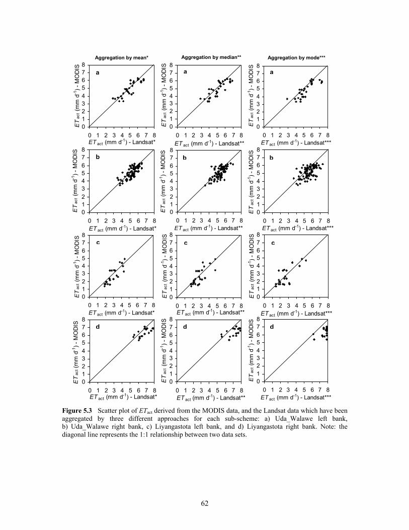
62

Figure 5.3 Scatter plot of ETact derived from the MODIS data, and the Landsat data which have been aggregated by three different approaches for each sub-scheme: a) Uda_Walawe left bank, b) Uda_Walawe right bank, c) Liyangastota left bank, and d) Liyangastota right bank. Note: the diagonal line represents the 1:1 relationship between two data sets.

a a a

b b b

c c c

d d d

Aggregation by mean* Aggregation by median** Aggregation by mode***

012345678

0 1 2 3 4 5 6 7 8ET act (mm d-1) - Landsat*

ET

act (

mm

d-1

) - M

OD

IS

012345678

0 1 2 3 4 5 6 7 8ET act (mm d-1) - Landsat**

ET

act (

mm

d-1

) - M

OD

IS

012345678

0 1 2 3 4 5 6 7 8ET act (mm d-1) - Landsat***

ET

act (

mm

d-1

) - M

OD

IS

012345678


ET

act (

mm

d-1

) - M

OD

IS

012345678


ET

act (

mm

d-1

) - M

OD

IS

012345678


ET

act (

mm

d-1

) - M

OD

IS

012345678


ET

act (

mm

d-1

) - M

OD

IS

012345678


ET

act (

mm

d-1

) - M

OD

IS

012345678


ET

act (

mm

d-1

) - M

OD

IS

012345678


ET

act (m

m d

-1) -

MO

DIS

012345678


ET

act (

mm

d-1

) - M

OD

IS

012345678


ET

act (

mm

d-1

) - M

OD

IS

63

Table 5.1 Comparisons of maximum, minimum, average, and coefficient of correlation of ETact values derived from the MODIS measurements and the Landsat measurements. Note: Absolute deviations, percentage deviations and the coefficient of correlation are denoted by Abs., % Dev., and *r respectively. Dimensionless percentage deviations are shown within brackets.

Value

ETact derived from MODIS

ETact derived from Landsat measurements; having sample aggregated by:

category Units measurements Mean Median Mode

Abs. %Dev. Abs. %Dev. Abs. %Dev.

Uda_Walawe left bank

Minimum mm d-1 3.3 2.9 (14) 2.9 (14) 2.9 (14)

Maximum mm d-1 6.3 6.7 (6) 6.9 (9) 7.3 (14)

Average mm d-1 4.9 5.0 (2) 5.1 (4) 5.4 (9)

*r - 0.87 0.85 0.84

Uda_Walawe right bank

Minimum mm d-1 3.5 3.5 (0) 3.5 (0) 3.7 (5)

Maximum mm d-1 6.3 6.5 (3) 7.0 (10) 7.3 (14)

Average mm d-1 5.1 5.3 (4) 5.4 (6) 5.6 (9)

*r - 0.75 0.67 0.55

Liyangastota left bank

Minimum mm d-1 1.4 1.9 (26) 1.7 (18) 1.5 (7)

Maximum mm d-1 4.9 4.4 (11) 4.8 (2) 5.2 (6)

Average mm d-1 2.7 3.0 (10) 2.8 (4) 2.7 (0)

*r - 0.85 0.76 0.75

Liyangastota right bank

Minimum mm d-1 4.6 5.4 (15) 5.5 (16) 6.2 (26)

Maximum mm d-1 7.1 7.9 (10) 8.0 (11) 7.9 (10)

Average mm d-1 6.3 6.7 (6) 7.0 (10) 7.6 (17)

*r - 0.68 0.62 0.53

64

Comparison of above results (Table 5.1) points out that the minimum, the maximum, and the average values of the aggregations performed by mean, median or mode values show deviations from 0% to 26%. However, the values derived from the aggregation by mean indicate the highest correlation.

The difference between the minimum values of the MODIS results and the Landsat results (derived through the aggregation by mean) shows a maximum of 26% in Liyangastota left bank that is in absolute terms 0.5 mm d-1. For such a small absolute deviation, the percentage deviation has taken a high value because of the low ETact values of the crop (i.e. 1.9 mm d-1

and 1.4 mm d-1). As per Irrigation Department records, on 14th of March 2001, paddy cultivation of the Liyangastota left bank was in the latter part of the late growth stage (wet season 2000-2001). To facilitate the paddy harvest, irrigation water is cut off during the latter part of the late growth stage. During this period, due to crop water stress condition, ETact takes low values. Under the same situation, the difference between the average values of the MODIS results and the Landsat results (derived through the aggregation by mean) shows a maximum of 10% in the the Liyangastota left bank scheme that is, in absolute terms 0.3 mm d-1 (i.e. from the difference of 3.0 mm d-1 and 2.7 mm d-1).

However, on 14th of March 2001, the Liyangastota right bank was in the beginning of the late stage of crop growth. Irrigation water is supplied to the cropped area. Therefore ETact has shown considerably high values. The difference between the average values of the MODIS results and the Landsat results (derived through the aggregation by mean) shows a maximum of 6% in the the Liyangastota right bank scheme.

In Sri Lanka, year 2000 was a drought year. Adequate water was not available in the Uda_Walawe reservoir to start the wet season of the year 2000-2001. Thus, following dry season was started in the beginning of the March, 2001. Land preparation takes nearly 4 weeks. On 14th of March 2001, lands may be partially prepared for the cultivation. Therefore, ETact has shown moderate values in both schemes under Uda_Walawe.

In most of the cases, the differences between the MODIS results and the Landsat results derived through the other categories (aggregation by median and mode), show percentage deviations higher than the values derived through the aggregation by mean values. The maximum and the minimum values are the two extremes of a sample distribution and do not represent the entire sample. The average is a good measure of central tendency for roughly symmetric distributions but can be misleading in skewed distributions since it can be greatly influenced by extreme scores. However, correlation is a statistical technique, which can show whether and how strongly pairs of variables are related.

In each sub-scheme, the Landsat measurements, which have been derived through aggregation by mean, have indicated the highest correlation when compared with the other two

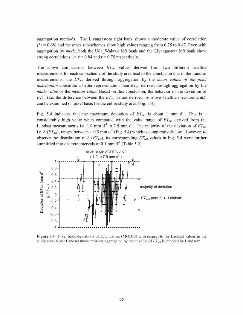
65

aggregation methods. The Liyangastota right bank shows a moderate value of correlation (*r = 0.68) and the other sub-schemes show high values ranging from 0.75 to 0.87. Even with aggregation by mode, both the Uda_Walawe left bank and the Liyangastota left bank show strong correlations i.e. r = 0.84 and r = 0.75 respectively.

The above comparisons between ETact values derived from two different satellite measurements for each sub-scheme of the study area lead to the conclusion that in the Landsat measurements, the ETact derived through aggregation by the mean values of the pixel distribution constitute a better representation than ETact derived through aggregation by the mode value or the median value. Based on this conclusion, the behavior of the deviation of ETact (i.e. the difference between the ETact values derived from two satellite measurements), can be examined on pixel basis for the entire study area (Fig. 5.4).

Fig. 5.4 indicates that the maximum deviation of ETact is about 1 mm d-1. This is a considerably high value when compared with the value range of ETact derived from the Landsat measurements i.e. 1.9 mm d-1 to 7.9 mm d-1. The majority of the deviation of ETact i.e. δ (ETact), ranges between ± 0.5 mm d-1 (Fig. 5.4) which is comparatively low. However, to observe the distribution of δ (ETact), its corresponding ETact values in Fig. 5.4 were further simplified into discrete intervals of 0.1 mm d-1 (Table 5.2).

Figure 5.4 Pixel basis deviations of ETact values (MODIS) with respect to the Landsat values in the study area. Note: Landsat measurements aggregated by mean value of ETact is denoted by Landsat*.

-1

-0.8

-0.6

-0.4

-0.2

0

0.2

0.4

0.6

0.8

1

0 1 2 3 4 5 6 7 8 9 10 11 12

value range of distribution( 1.9 to 7.9 mm d-1)

majority of deviation

Dev

iatio

n of

ET

act (

mm

d-1

)

δ (E

Tac

t)

ET act (mm d-1) - Landsat*

66

Table 5.2 Variation of resulting ETact values derived from the Landsat measurements with respect to the incremental change of δ (ETact) by 0.1 mm d-1 of discrete intervals.

Variation of resulting ETact values derived

from Landsat data Incremental changes

of δ (ETact) mm d-1

% Cumulative %

0 5 5

0.1 18 23

0.2 8 31

0.3 16 47

0.4 11 58

0.5 9 67

0.6 12 79

0.7 5 84

0.8 6 90

0.9 5 95

1.0 5 100

The above analysis shows that the deviation of ETact from 0 to 0.2 mm d-1 represents 31% of the pixel distribution in the study area, and the deviation from 0 to 0.5 mm d-1 represents 67% of the distribution which is two third of the entire study area. In addition, the top most deviation i.e. ranges from 0.8 mm d-1 to 1.0 mm d-1 acquires only 5% of the study area.

5.2.2 Impact of error of ETact due to the spatial resolution on management decisions

It is necessary to assess how the error component of ETact would affect the management decisions of irrigation practices in Sri Lanka. ETact or the crop water use is essential in both planning and implementing (including controlling) stages of irrigation management. Following conclusions are used assess the impact of the error component of ETact.

• Under water stressed situations (i.e. crop without irrigation water), ETact derived from the MODIS measurements (through SEBAL algorithm) have deviated 10% from those derived from the Landsat measurements.

• Under normal situations (i.e. crop with irrigation water) this deviation has reduced to 6% and below.

Therefore in estimation of evapotranspiration, it is much more accurate to use the MODIS measurements acquired on daily basis even with the deviations of 10% or less. At the

67

implementing stage of a cultivation season, it is important to assess the impact of these deviations on the water deliveries.

When compared to the negligible downloading cost and the high frequency of the MODIS measurements, this approach is more feasible for the country. Hence, the ETact values measured by the MODIS measurements with these deviations are sufficiently accurate for irrigation management decisions in large scale irrigation schemes in Sri Lanka.

In order to validate, remote sensing measurements, a larger aperture scintillometer (LAS) was arranged to measure the sensible heat flux density H with a net radiometer (NR-LITE) to measure the net radiation Rn. The transmitter was installed on top of a 12 m high steel tower at an elevation of 20 m above the paddy fields and at a distance of 1200 m from the receiver. The height of 20 m was needed to transmit over the top of the palm trees. Often, however, the ocean wind was blowing hard across the flat irrigated area. For a small twist of the steel structure (i.e. an angle ~ 0.0050) due to wind, the transmitted beam shifted out of range from the 100 mm diameter receiver. Also, local monkeys frequently interfered with the position of the instruments. As a result, the scintillometer could not be used to validate evapotranspiration results in this study. However, using the same instrument, the SEBAL outputs derived by NOAA satellite images (with similar band characteristics of the MODIS) were validated in Sri Lanka from December 1999 – February 2000. During this period, the transmitter and the receiver were fixed on two hills being 1900 m apart. The test area in the latter study consisted with mainly paddy and mixed vegetation. The difference between 10 day ETact estimates from the SEBAL computation and the scintillometer measurements averaged 17% (Hemakumara et al., 2003). For future studies in coastal plains it is suggested to use a shorter distance between the transmitter and receiver so that a beam can be transmitted without disturbance by trees. The use of the scintillometer to validate remotely sensed evapotranspiration is promising in areas where wet and dry pixels are not present (Gieske and Meijninger 2005).

68

5.3 Constitution of errors due to variation of ground cover area in estimation of ETact using the MODIS measurements

In the analysis using satellite measurements, distribution of the resulting values is always confined to the pixel size, which determines the precision of homogeneity. However, due to the undulations of the topography, the spatial distribution of the farm allotments over the command area never emerges as a uniform pattern. The smallest extent of the individual farm allotment in the study area is 1 ha and about 10 to 30 of such allotments are fed by each field canal of the irrigation system. A set of farm allotments attached to each field canal is treated as a smallest operational unit of the command area, which is managed by the respective farmer organization. Several of such field canals are connected to one distribution canal of the system. The water institution manages the operational control of water from the main water source to the distribution canal level.

Based on the farm allotments, which were distributed over the canal system (i.e. the block-out plan of the command area), the water distribution is carried out. In order to perform ETact computation based on satellite measurements, the irregular shaped water distribution areas could be replaced by a set of square shaped pixels. Some of these pixels along the periphery may be positioned partially outside the demarcated boundary. The values of such pixels contain the properties of the land cover immediately beyond the concerned area. The effect of boundary pixels may be varying due to the prevailing field condition of the surrounding area (Fig. 5.5).

In order to define a feasible extent for the MODIS measurements (ETact), following two conditions have to be considered.

1) When the area concerned is too small (Fig. 5.5a) compared with the low resolution of the MODIS measurements, the impact of boundary pixels on the final output value should be optimum i.e. a feasible extent. due to the pixel size

2) When the area concerned is too large (Fig. 5.5c) compared with the heterogeneity of the land cover (i.e. site specific condition), the effect due to the variations of the pixel values should be optimum i.e. a feasible extent due to the heterogeneity of land cover.

These two limits have to be defined by observing the variations of the error component of ETact derived from the MODIS measurements, when the spatial extent of the land cover is varied. Hence, a sample analysis has to be carried out to determine such variations of the error component against the spatial extent.

69

Figure 5.5 Effect of boundary pixels when they are mixed with the area at the outside of the concerned area: a) area concerned is considerably small and mixed pixels dominate, b) area concerned is moderately large and inner pixels dominate, and c) area concerned is too large and heterogeneity of the inner pixels dominates.

5.3.1 Approach to determine the error component of ETact with respect to the area of ground cover

For the sample analysis, 16 adjoining pixels (the sample size) were selected from the SEBAL output map of ETact obtained through the MODIS measurements. These pixels represent 1600 ha of the ground cover. This extent is quite small when compared to the 100 ha size of the MODIS pixel. Therefore, the sample analysis is started from the spatial extent of 1600 ha. Then the error component has to be determined.

The out puts of the 16 values were averaged to obtain the observed value (i.e. random variable). In order to represent the same spatial extent, one single effective value has been derived through the SEBAL process in such a way that the relevant spectral values have been aggregated by their mean values before subjected to the SEBAL process (see Fig. 5.2a). Thus, this effective value exhibits a fair representation of the sample and it can be regarded as an ordinary variable. The error component can be defined as the difference between the effective value and the observed value. However, one small sample cannot make a fair representation of a large land cover. In order to make an unbiased representation, the entire procedure is repeated for a cloud free data samples (n = 324) having the same sample size of 16 pixels, covering a large part of southern Sri Lanka. Thus, the error component of the entire population has to be estimated (Fig. 5.6).

Mixed pixels along the boundary

Different land cover types inside the concerned area

Boundaries of the concerned areas

(a) (b) (c)

Mixed pixels along the boundary

Different land cover types inside the concerned area

Boundaries of the concerned areas

(a) (b) (c)

70

Figure 5.6 Proposed approach to determine the error component of ETact with small samples of similar size.

5.3.2 Estimation of error of ETact due to variations of land cover through regression analysis

Since the random variable distribution cannot be expected to be normal, the Gaussian distribution function is not applicable for error estimation. Hence, linear regression analysis is applied for the two output data sets in which the observed values would become the dependent variables and the corresponding effective values would become the independent variables. Thereby, predicted values for the random variables are computed by the regression model (e.g. Kothari, 1978; Ross, 1996). For any given value x of the independent variable, the random variable y is the dependent variable and the predicted value can be expressed as:

xBAyE )( += 5.2

The values A and B are to be estimated using the observed and the effective values. The estimated relationship takes the form:

ii β xy +α= 5.3

where α and β are the estimated values from the selected sample representing A and B respectively (Fig. 5.7).

Repeat the process for different data samples with the same sample size

Spectral aggregation

SEBAL SEBAL

16 pixels (MODIS)

Validate two data setsby linear regression

16 output values

One single effective value

Repeat the process for different data samples with the same sample size

Spectral aggregation

SEBAL SEBAL

16 pixels (MODIS)

Validate two data setsby linear regression

16 output values

One single effective value

71

Figure 5.7 Linear regression model for error estimation.

Since the density of the dependent variables yi is not specified as normal, a method such as maximum-likelihood estimators cannot be applied to determine α and β . In a situation like this, the least-squares method of estimation can be utilized (Mood and Grabill, 1963). The square deviation (Q) of the observed values (i.e. variance of the observed values) can be expressed as:

2

1)] ( [(

2)-(1 xy

nQ

n

ii βα +−= ∑

=

5.4

where n is the number of observations (sample size) and (n-2) is referred to as the degree of freedom of the distribution. In order to obtain the minimum square deviation (Qmin), the corresponding α and β can be estimated by applying the principle of least squares. The value of Qmin could be obtained by setting the partial derivatives with respectα and β to 0

i.e. 0),(=

∂∂

αβαQ and 0),(

=∂

∂ββαQ . Hence,

0 )] ([( 2 =β+α−− ∑=

in

ii xy

1

5.5

0 )] ([( 2 =β+α−− ∑=

in

iii xyx

1

5.6

The mean values of yi and xi could be expressed as ynyn

ii =∑

=1 and xnx

n

ii =∑

=1 respectively.

By substituting the mean values of yi and xi, the Eqs.5.5 and 5.6 can be rearranged as:

0 - - =βα xnnyn 5.7

0

2

4

6

8

0 1 2 3 4 5 6 7 8Effective value (independent variable)

Obs

erve

d va

lue

(d

epen

dent

var

iabl

e)

value predicted )](,[ ii βxαx +

line regression ii βxαy +=

)]([ ii βxαy +−

value predicted and value observed between difference

X

Y

value observed ),( ji yx

72

0 - - 2 =βα ∑∑==

n

iii

n

ii xxnyx

11

5.8

By solving Eqs.5.7 and 5.8, β values are obtained as:

∑

∑

=

== n

ii

n

iii

xnx

yxnyx

1

22

1

-

- β

5.9

Since 0)( =−∑=

xxn

ii

1, β and α can be simplified respectively as:

∑

∑

=

== n

ii

n

iii

xx

xxy

1

2

1

) - (

) - ( β

5.10

xxx

xxyy n

ii

n

iii

) - (

) - (

1

2

1

−=

∑

∑

=

=α

5.11

By substituting the values of α and β into Eq. 5.4, the least-square deviation Qmin is obtained. The “square-root of Qmin” would be the error of the observed values q for the selected size of the spatial extent i.e. Qmin = q2.

5.3.3 Behavior of the error component of ETact due to variation of the spatial extent

In order to determine the behavior of the error of the observed values q with respect to the spatial variations, the process was executed as follows:

i) Using the same SEBAL output map of ETact, the sample size was increased from 16 pixels to 144 pixels by discrete intervals i.e. 144 pixels represent 14400 ha. When compared with the extent of the largest sub-scheme of the study area i.e. Uda_Walawe right bank area with 10500 ha of spatial extent, 14400 ha can be considered as a large extent.

ii) The process described in (i) was repeated for three data sets of the MODIS measurements. For this statistical analysis, 324 samples of 16 pixels were selected. Hence, the population has a spatial extent of 5184 km2 covering a large part of the

73

south-east Sri Lanka, as well as several land cover and land use types. The three data sets were selected to represent the period of three growth stages of paddy (i.e. initial, development, and middle) within a cultivation season and the behavior of the error was determined. The results are graphically illustrated in Fig. 5.8a in which two limits of the error component of ETact due to the pixel size and the heterogeneity of the ground cover respectively are explained in next section.

Error component of the slope coefficient of linear regression: Furthermore, the estimated slope coefficient (i.e. β ) of the linear regression determines the increment of the predicted value due to the increase of effective value by one unit. The error component of the slope coefficient (Sβ) indicates the rate of change of error due to the prediction using the linear regression. The Eq. 5.10 can be re-arranged as (e.g. Guttman et al., 1971; Bowker and Lieberman, 1959):

∑=

=n

iii yc

1 β

5.12

where the values of ci are known constants because of the values of xi are already known. The variance or the least squares deviation of yi is q2 and it remains constant for all xi. Then the variance of β can be expressed as;

2

1

2 )var( qcn

ii∑

=

=β

∑=

=n

ii )xx(

q

1

2

2

-

5.13

The error of β is the square root of the variance and can be expressed as:

∑=

=n

ii xx

qS

1

2) - ( β

5.14

In order to determine the behavior of the error component of the slope coefficient Sβ, the process described in section 5.3.3 (i) and (ii) is repeated (Fig. 5.8b).

Quality assessment of least squares fitting: The quality of the error component due to the interdependence between two variables is given by the coefficient of correlation (e.g. Kothari, 1978). Though the correlation coefficient (r) is a quantitative indicator, it describes the quality of least squares fitting of the observed values and the effective values:

74

∑ ∑

∑

= =

==n

i

n

iii

n

iii

yyxx

yyxxr

1 1

22

1

) - () - (

) -)( - (

5.15

The behavior of the correlation coefficient is observed by repeating the process described in section 5.3.3 (i) and (ii) is repeated (Fig. 5.8c).

75

Figure 5.8 Two limits to define a feasible extent (i.e. due to the pixel size and the heterogeneity of the land cover) of land cover using MODIS measurements of 1000 m ×1000 m pixel size: a) behavior of the error component of ETact, b) behavior of the slope error of ETact, and c) behavior of the correlation between the observed and the effective values of ETact.

0.10

0.15

0.20

0.25

0.30

0.35

0.40

0.45

0 1 2 3 4 5 6 7 8 9 10 11 12 13 14 15 16Extent of sample area (103 ha)

Erro

r of E

Tac

t (m

m d

-1)

0.000.010.020.030.040.050.060.070.08


Slo

pe e

rror o

f ET

act (-)

0.900.910.920.930.940.950.960.970.98


Coe

ffici

ent o

f cor

rela

tion

(-)

a

b

c

erro

r due

to p

ixel

si

ze in

crea

ses

erro

r due

to

hete

roge

neity

of t

he

land

cov

er in

crea

ses

initial stage

development stage

middle stage

middle stage

middle stage

initial stage

initial stage

development stage

development stage

erro

r due

to p

ixel

si

ze in

crea

ses

erro

r due

to p

ixel

si

ze in

crea

ses

erro

r due

to

hete

roge

neity

of t

he

land

cov

er in

crea

ses

erro

r due

to

hete

roge

neity

of t

he

land

cov

er in

crea

ses

feasible extent

feasible extent

feasible extent

76

5.3.4 Discussion on feasible extent for ETact estimation using the MODIS measurements

As shown in Fig. 5.8a, when the spatial extent is increased, the error of ETact sets off to decrease since the majority of the inner pixels of the area concerned begin to compensate the adverse effect of mixed pixels along the periphery. When the spatial extent is further increased, the error of ETact reaches to its minimum and thereafter starts to increase. The subsequent increasing trend of the error component justifies that the heterogeneity of pixel values distributed over the area concerned (i.e. site specific condition) has deteriorated the final output. Subject to these two conditions (also stipulated in section 5.3), the land cover area which determines the minimum error of ETact would be the optimal spatial extent for the MODIS pixels of 1000 m.

However from the application point of view, it is difficult to stick all computations to a particular limiting value of the area concerned. Hence, based on this optimal extent, it is required to establish a suitable range of extent i.e. a feasible extent. By observing deflection points of the curves closer to the optimal extent from either side, two limits of land cover were selected to represent the boundaries of a feasible extent (Fig. 5.8a). The lower limit is subjected to the MODIS measurements of 1000 m spatial resolution whereas the upper limit is subjected to the heterogeneity of the land cover due to site specific conditions. Thus, by considering two limits, the boundaries of the feasible extent can be set as 2000 ha and 4000 ha respectively.

Within this range, the magnitude of the error of ETact shows its values less than 0.3 mm d-1. As shown in section 5.2.1, the estimated values of potential evapotranspiration for paddy vary between 4 mm d-1 and 7.5 mm d-1. Hence, a 0.3 mm d-1 error of ETact computes 7.5% and 4% of the estimated potential evapotranspiration values respectively (i.e. error of ETact / ETpot). These percentage error values are considerably low when compared with the pixel resolution of 1000 m.

As in the previous case, when spatial extent increases, the slope error of the linear regression also indicates an increasing trend with fluctuations (Fig. 5.8b). Therefore, the same procedure was followed to demarcate the two boundaries. Also in this case, the feasible extent was found to be as close as to the previous case. For this feasible extent, Fig. 5.8b shows that the slope error of ETact is less than 3%. This clarifies that in the error estimation of ETact, for a unit increment of the effective value (within the feasible extent through a linear regression), the error of ETact is changed by less than 3%. Fig. 5.8b shows that even for an extent of 14500 ha, the slope error of the linear regression model has reached a maximum of 7%, which is a considerably low value. Thus, for the feasible extent with the MODIS measurements of 1000 m spatial resolution, the linear regression model is acceptable.

77

Moreover, when the spatial extent is increased, the correlation between the observed values and the effective values of the ETact, shows an decreasing trend with fluctuations in each growth stage (Fig. 5.8c). This reveals that for the low values of the spatial extent, the correlation coefficient takes high values. As in the earlier two cases, the feasible extent varies between 2000 ha and 4000 ha. For this feasible extent, the correlation between the observed values and the effective values of the ETact has exceeded 94% showing a strong correlation.

When the error due to the heterogeneity of the land cover is concerned, there are site specific conditions such as cultivation pattern, growth stage, land use, soil type and vegetation type, which can be varied with spatial and temporal changes. However in this statistical analysis, the selected population covers a large part of the south-east Sri Lanka. The major land cover types are paddy, tea, coconut, and tropical forest whereas the major land use types are irrigated and rain fed agriculture, and urban areas. The climate and the soil types are as described in section 2.2 and 2.3. In the context of Sri Lanka, the recommended range of feasible extent (i.e. 2000 ha to 4000 ha) for the MODIS measurements of 1000 m spatial resolution has a wide range of variety in the topography. However in the global context, to ensure error due to the heterogeneity of land cover, it is recommended to carry out a sample study based on the land cover variation.

79

6. Assessing strategic performance in the Liyangastota scheme

6.1 Implementation of performance assessment

Strategic performance is assessed considering the water balance components depicted in Fig. 6.1 for the Liyangastota sub-schemes, using indicators selected in Table 3.2. Two examples of assessing irrigation performance, one for the Liyangastota right bank during wet season of 2002-2003 and the other one for the same scheme during dry season of 2003, are described in this chapter. To quantify ETact , 34 MODIS images were used for the wet season 2002-2003 and 24 images were used for the dry season 2003. A water use matrix for irrigated crops is introduced to describe how effectively the irrigation manager has supplied irrigation water to reduce the crop water stress. Processed field-data received on daily basis from each sub_scheme and stored in a digital database, were used for the analysis. The values of ETact, and grain yield derived from the satellite measurements were combined with the field measurements. To estimate ETpot, daily weather data was associated with the satellite measurements. Socio-economic performance of both the schemes (Liyangastota and the Uda_Walawe) is assessed in next chapter.

Figure 6.1 Schematic representation of flows in the water balance of an irrigated area.

re-use in a cascade system

river diversion

from a reservoir

Irrigation supply,Vc

Precipitation (gross), P

ground water flow from upstream

ground water flow to river

Drainage, Vdr

Drainage, Vdr depression / lakesea

ETact from the area



river diversion

from a reservoir

Irrigation supply,Vc

Precipitation (gross), P

ground water flow from upstream

ground water flow to river

Drainage, Vdr

Drainage, Vdr depression / lakesea

ETact from the area

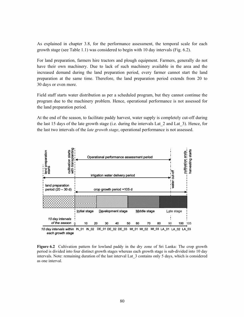
80

As explained in chapter 3.8, for the performance assessment, the temporal scale for each growth stage (see Table 1.1) was considered to begin with 10 day intervals (Fig. 6.2).

For land preparation, farmers hire tractors and plough equipment. Farmers, generally do not have their own machinery. Due to lack of such machinery available in the area and the increased demand during the land preparation period, every farmer cannot start the land preparation at the same time. Therefore, the land preparation period extends from 20 to 30 days or even more.

Field staff starts water distribution as per a scheduled program, but they cannot continue the program due to the machinery problem. Hence, operational performance is not assessed for the land preparation period.

At the end of the season, to facilitate paddy harvest, water supply is completely cut-off during the last 15 days of the late growth stage (i.e. during the intervals Lat_2 and Lat_3). Hence, for the last two intervals of the late growth stage, operational performance is not assessed.

Figure 6.2 Cultivation pattern for lowland paddy in the dry zone of Sri Lanka: The crop growth period is divided into four distinct growth stages whereas each growth stage is sub-divided into 10 day intervals. Note: remaining duration of the last interval Lat_3 contains only 5 days, which is considered as one interval.

land

pre

para

tion

star

ts

culti

vatio

n st

arts

w

ith tr

ansp

lant

ing

irrigation water delivery period

crop growth period =105 d

Initial stage Development stage Middle stage

land preparation period (20 – 30 d) w

ater

cut

-off

0

10

IN_01 IN_02 DE_01 DE_02 DE_03 MI_01 MI_02 MI_03 LA_01 LA_02 LA_03IN_01 DE_01 MI_02DE_03 LA_01 LA_03MI_03IN_02 MI_01DE_02 LA_02

30 40 50 60 70 80 1002010

Late stage

culti

vatio

n en

dsha

rves

ting

star

ts

10 day intervals of the season

10 day intervals within each growth stage

1050 90

Operational performance assessment period

land

pre

para

tion

star

ts

culti

vatio

n st

arts

w

ith tr

ansp

lant

ing

irrigation water delivery period

crop growth period =105 d

Initial stage Development stage Middle stage

land preparation period (20 – 30 d) w

ater

cut

-off

0

10

IN_01 IN_02 DE_01 DE_02 DE_03 MI_01 MI_02 MI_03 LA_01 LA_02 LA_03IN_01 DE_01 MI_02DE_03 LA_01 LA_03MI_03IN_02 MI_01DE_02 LA_02

30 40 50 60 70 80 1002010

Late stage

culti

vatio

n en

dsha

rves

ting

star

ts

10 day intervals of the season

10 day intervals within each growth stage

1050 90

Operational performance assessment period

81

6.2 The target values and the critical values for water balance indicators

For the indicators in Table 3.2, target levels to assess the performance need to be determined. In the assessment stage, the performance above target is considered as good performance or over performance. However, if the performance is slightly below this set target level performance may not be considered poor. Therefore, a justifiable tolerance margin is allowed below the target level for each performance indicator (Fig. 6.3). The lower limit of the transition range is referred to as the critical level. The performance below the critical level is considered as poor performance (i.e. under performance). Both the target level and the critical level are subject to local conditions.

Figure 6.3 Terminology on indicator related levels and ranges within the performance indicator value.

Poor performance(under performance)

Good performance(over performance)

Target level

Critical level

Perfo

rman

ce in

dica

tor v

alue

Tolerance margin Transition range

Poor performance(under performance)

Good performance(over performance)

Target level

Critical level

Perfo

rman

ce in

dica

tor v

alue

Tolerance margin Transition range

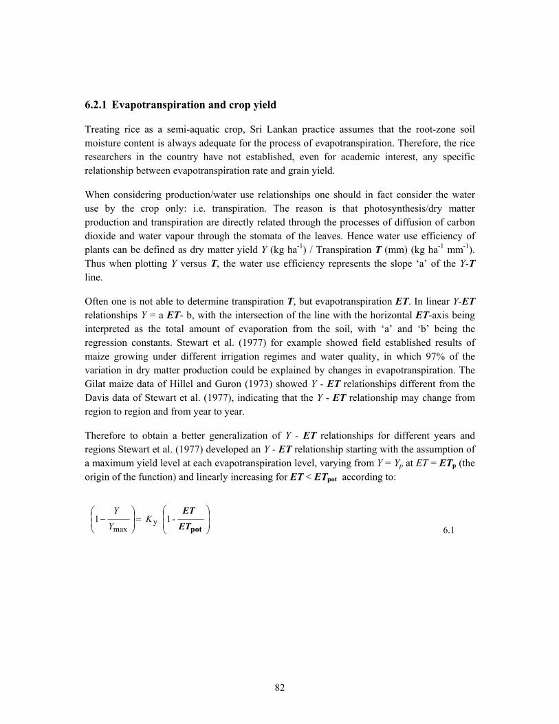
82

6.2.1 Evapotranspiration and crop yield

Treating rice as a semi-aquatic crop, Sri Lankan practice assumes that the root-zone soil moisture content is always adequate for the process of evapotranspiration. Therefore, the rice researchers in the country have not established, even for academic interest, any specific relationship between evapotranspiration rate and grain yield.

When considering production/water use relationships one should in fact consider the water use by the crop only: i.e. transpiration. The reason is that photosynthesis/dry matter production and transpiration are directly related through the processes of diffusion of carbon dioxide and water vapour through the stomata of the leaves. Hence water use efficiency of plants can be defined as dry matter yield Y (kg ha-1) / Transpiration T (mm) (kg ha-1 mm-1). Thus when plotting Y versus T, the water use efficiency represents the slope ‘a’ of the Y-T line.

Often one is not able to determine transpiration T, but evapotranspiration ET. In linear Y-ET relationships Y = a ET- b, with the intersection of the line with the horizontal ET-axis being interpreted as the total amount of evaporation from the soil, with ‘a’ and ‘b’ being the regression constants. Stewart et al. (1977) for example showed field established results of maize growing under different irrigation regimes and water quality, in which 97% of the variation in dry matter production could be explained by changes in evapotranspiration. The Gilat maize data of Hillel and Guron (1973) showed Y - ET relationships different from the Davis data of Stewart et al. (1977), indicating that the Y - ET relationship may change from region to region and from year to year.

Therefore to obtain a better generalization of Y - ET relationships for different years and regions Stewart et al. (1977) developed an Y - ET relationship starting with the assumption of a maximum yield level at each evapotranspiration level, varying from Y = Yp at ET = ETp (the origin of the function) and linearly increasing for ET < ETpot according to:

=

−

potET

ET-1 1 y

maxK

Y

Y

6.1

83

where Ky is the dimensionless slope to be determined from field experiments, for which the quantities (being the maximum attainable yield), ETpot, Y and ET have to be calculated/measured. Doorenbos and Kassam (1979) have analyzed Y - ET relationships in great detail for some 26 crops, distinguishing also between various growth periods being sensitive for water deficits.

Eq. 6.1 has further being used in this thesis to predict the reduction in grain yield of rice when a shortage of soil water would cause crop stress. In Eq. 6.1, Y can be replaced by Yact which is the actual grain yield (kg ha-1). Thereby, Ymax becomes the maximum attainable grain yield (kg ha-1). ET, can be replaced by ETact , which is the time integrated actual evapotranspiration over the season. Thus, ETpot becomes the time integrated potential evapotranspiration over the season.

Values of Ky in Eq. 6.1 vary between 0.7 and 1.35 (FAO 56, 1998). But for most of the crops, the seasonal Ky is nearly 1. Thus, for crops with Ky unknown, as is true for this study, Ky =1 is recommended for use (FAO 56, 1998). However, it is necessary to establish a more realistic crop-water production function for paddy in Sri Lanka by considering its growth related factors such as crop variety, seasonal weather condition etc.

Fig. 2.5 shows the average seasonal grain yield of a part of the study area (70 % of the study area) being presented for 15 years, starting from 1979. In most of the seasons, the average grain yield reached 4.8 ton ha-1 (i.e. the mode value of the frequency distribution) showing a maximum of 6 ton ha-1. Considering the difficulty in reaching the maximum average grain yield in all the seasons by every farmer, the target value of the grain yield can be set as 5 ton ha-1 i.e. just above the mode value of the grain yield during the last 15 years in the part of the study area. To reach this grain yield target, it is required to derive the corresponding level of ETact /ETpot to be maintained over the irrigated area.

To establish a critical level for the grain yield, two major factors have been considered: Farmer’s return on paddy cultivation investment and maintaining a stable price of rice to protect the consumer.

As indicated in section 1.2, from the year 2000 to 2005 to reach self-sufficiency in rice nationally, the national average grain yield has to be increased from 3.7 ton ha-1 to 4.1 ton ha-1. The Government needs to maintain this near self-sufficiency level of rice to fulfill the consumer’s demand because the majority of the population comes under low income category. When the supply level meets the consumer’s demand, as indicated in Fig. 6.4a, the price level will be stabilized.

At present, seasonal cultivation cost of paddy is about 54,000 SLR ha-1 (1 $ = 100 SLR, Sri Lankan Rupee) whereas farm gate price for paddy offered by the Government is 15.50 SLR kg-1 (e.g. MONLAR, 2005). Hence, to recover the investment cost (i.e. to reach the break

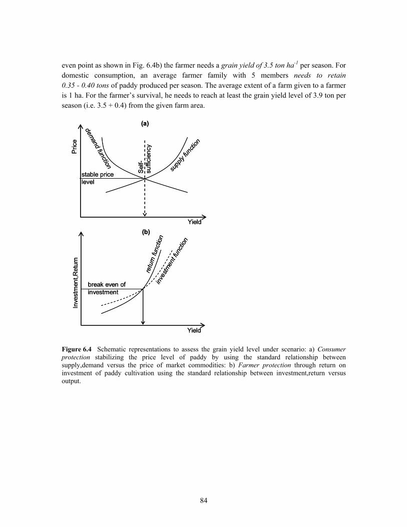
84

even point as shown in Fig. 6.4b) the farmer needs a grain yield of 3.5 ton ha-1 per season. For domestic consumption, an average farmer family with 5 members needs to retain 0.35 - 0.40 tons of paddy produced per season. The average extent of a farm given to a farmer is 1 ha. For the farmer’s survival, he needs to reach at least the grain yield level of 3.9 ton per season (i.e. 3.5 + 0.4) from the given farm area.

Figure 6.4 Schematic representations to assess the grain yield level under scenario: a) Consumer protection stabilizing the price level of paddy by using the standard relationship between supply,demand versus the price of market commodities: b) Farmer protection through return on investment of paddy cultivation using the standard relationship between investment,return versus output.

retu

rn fu

nctio

nin

vestm

ent fu

nctio

n

Inve

stm

ent,R

etur

n

Yield

break even of investment

Pric

e

supp

ly fun

ction

demand function

Yield

stable price level

(a)

(b)

Sel

f-su

ffici

ency

retu

rn fu

nctio

nin

vestm

ent fu

nctio

n

Inve

stm

ent,R

etur

n

Yield

break even of investment

Pric

e

supp

ly fun

ction

demand function

Yield

stable price level

(a)

(b)

Sel

f-su

ffici

ency

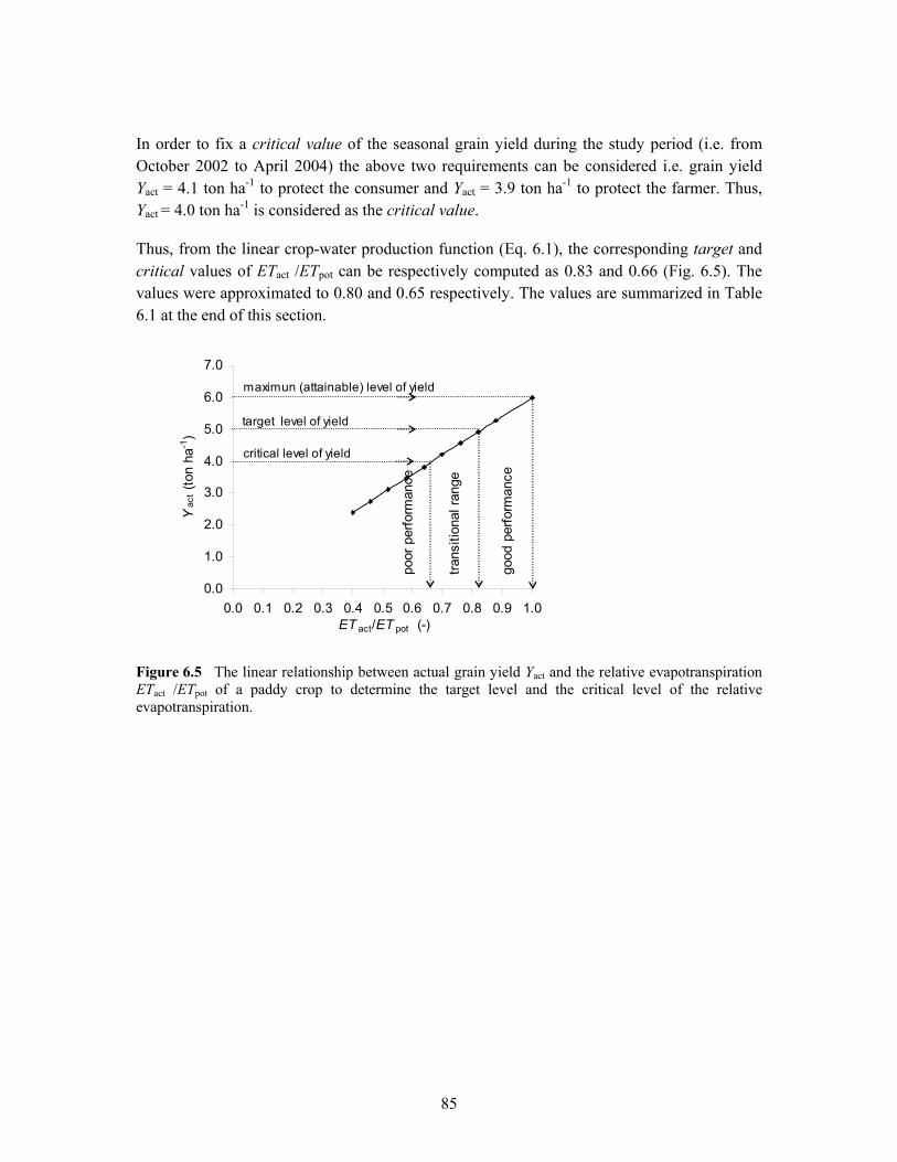
85

In order to fix a critical value of the seasonal grain yield during the study period (i.e. from October 2002 to April 2004) the above two requirements can be considered i.e. grain yield Yact = 4.1 ton ha-1 to protect the consumer and Yact = 3.9 ton ha-1 to protect the farmer. Thus, Yact = 4.0 ton ha-1 is considered as the critical value.

Thus, from the linear crop-water production function (Eq. 6.1), the corresponding target and critical values of ETact /ETpot can be respectively computed as 0.83 and 0.66 (Fig. 6.5). The values were approximated to 0.80 and 0.65 respectively. The values are summarized in Table 6.1 at the end of this section.

Figure 6.5 The linear relationship between actual grain yield Yact and the relative evapotranspiration ETact /ETpot of a paddy crop to determine the target level and the critical level of the relative evapotranspiration.

0.0

1.0

2.0

3.0

4.0

5.0

6.0

7.0

0.0 0.1 0.2 0.3 0.4 0.5 0.6 0.7 0.8 0.9 1.0 ET act/ET pot (-)

Yac

t (to

n ha

-1)

target level of yield

critical level of yield

maximun (attainable) level of yield

trans

ition

al ra

nge

good

per

form

ance

poor

per

form

ance

86

6.2.2 Delivery performance ratio

The delivery performance ratio is defined as:

intc,

c water of flow Intended waterof flow Actual

VV

=

6.2

Amount of Irrigation water to be delivered from the main source (i.e. the reservoir or the river diversion) Vc,int can be expressed as (Bos and Nugteren, 1990; ICID, 1978):

condisapp

e,antmintc, εεε

PVV

−=

6.3

where Vm is the amount of irrigation water needed and made available for evapotranspiration of the crop in order to avoid undesirable water stress in the plants throughout the growing cycle, Pe,ant is the effective use of anticipated rainfall, εapp is the application efficiency of the irrigated water from the field inlet to the crop, εdis is the distribution efficiency of the canal system from the off-takes of the distribution canal to the field inlet, εcon is the conveyance efficiency of the main canal system from its main source to the off-takes of the distribution canal, and Pe,ant is the effective use of anticipated rainfall computed using a semi-empirical method developed by the U.S. Department of Agriculture in 1970 (e.g. Bos and Nugteren, 1990). For large irrigation schemes in Sri Lanka, recommended values for εapp and εdisεcon are 0.6 and 0.7 respectively. Real rainfall records and computed values of actual precipitation and anticipated precipitation are given in Appendix A. ETact and ETpot values derived from MODIS images for the Liyangastota right bank are given in Appendix B.

To establish target and critical values, the following approach is adopted.

• The irrigation manager as well as the farmer intends to achieve the highest attainable grain yield of 6 ton ha-1 even though there are difficulties. Corresponding to this grain yield level, the ETact /ETpot = 1.0 (see Fig. 6.5). The computed annual average values of ETpot and Pe,ant were 5.4 mm d-1 and 1.2 mm d-1 respectively (see Appendix C). Thus, from Eq. 6.3, the intended irrigation water supply (Vc,int) can be computed as 10 mm d-1.

• Since all the farmers cannot achieve the highest attainable grain yield level, the target value of the grain yield has been set at 5 ton ha-1. From Fig. 6.5, the corresponding ETact /ETpot = 0.83. To compute the target value of the irrigation water supply, the term ETpot in Eq. 6.3 is replaced by ETact (= 0.83 ETpot) and computed as 7.8 mm d-1. The

87

irrigation manager should make the necessary arrangements to maintain the water deliveries i.e. the actual irrigation water supply, above this target level.

• Representing the efforts to protect the farmer as well as the consumer, the critical level of grain yield has been set at the level of Yact = 4.0 ton ha-1. From Fig. 6.5, the corresponding ETact /ETpot = 0.67. Following the procedure explained in the previous step, the critical value of the irrigation water supply Vc can now be computed as 5.8 mm d-1. If the actual irrigation water supply is reduced to this critical value, rice yield decreases to its critical level.

Substituting the values of the irrigation water supply from the above three steps into Eq. 6.2, the corresponding target value and the critical value of the delivery performance ratio Vc /Vc,int can be computed as 0.8 and 0.6 respectively. The target level of the delivery performance ratio is set as Vc /Vc,int = 0.80.

The critical level determines a safety margin for the target level (i.e. a tolerance margin). To control this safety margin in this study, the computed value of the critical level of the delivery performance ratio Vc /Vc,int was approximated to 0.65 to start the performance assessment. The target and critical values are summarized in Table 6.1 at the end of this section.

The manager plans to deliver his intended amount of irrigation water, with the anticipation of rain on the cropped area. When the situation is ideal Vc /Vc,int = 1. If the delivery performance ratio Vc /Vc,int exceeds 1, it indicates over-supply of irrigation water. Therefore, the values of the delivery performance ratio Vc /Vc,int > 1 are considered as undesirable, subjected to the anticipated rainfall i.e. excess water deliveries from the main source when compared to the ideal situation.

6.2.3 Drainage ratio

The drainage ratio is defined as:

PVV

area theinto entering water Totalarea from water drainage Total

c

dr+

=

6.4

In large scale gravity-irrigation systems in Sri Lanka with un-lined canals, a huge amount of water flows through drainage canals (Fig. 6.6). In the study area about 10% of the irrigation water flows through to the main drainage canals (ID, 2002). Therefore, the target value of the drainage ratio Vdr /(Vc + P) is set as 0.10.

88

Figure 6.6 Drainage canal in the cropped area with water level close to its bund top level.

In addition, when it rains, a substantial amount of rainfall runoff from the surrounding highlands accumulates in the drainage canals. Because there is no separate drainage system for the highlands, this drainage volume is included in the drainage flow of the study area. As the drainage ratio Vdr /(Vc + P) is a dimensionless indicator, the variation of the ratio Vdr /(Vc + P) is more appropriate in the assessment than to compare the values in absolute terms.

While fixing a critical value for the drainage ratio Vdr /(Vc + P), its impact on the cultivation has to be considered. Hence, situations such as downstream flood level and extent of water logging areas are not considered. Related to the irrigation performance, the following cases causing drainage ratio Vdr /(Vc + P) to increase, are considered as follows.

case 1). Due to operational deficiencies in the water distribution system, the inflow rate at the off-take would be higher than the outflow rate of the canal outlets. Such situations can be frequently observed in the distributary canals. The canal water level increases and thereby a portion of water overtops the canal banks along their weak sections and accumulates into the drainage system. In addition, due to such deficiencies, some areas may get more water than required. The excess water overtops the small field bunds in the cropped area and some are breached. Consequently, more irrigation water flows into the drainage canals. The farmer organizations carry out the field level (i.e. tertiary level) water distributions and their shortcomings in water distribution also causes the drainage water to increase. The overall outcome would be the increase of drainage water by decreasing the available water for the crop.

water level

flow

Drainage canal

Paddy fields

water level

flow

Drainage canal

Paddy fields

89

case 2). The drainage volume increases due to the defects of the canal system such as canal breaches because of the movement of cattle, water leaks along the sections where the canal is formed on an earth fill (i.e. canal bed level is above the ground level). In earthen canals, weeding of bunds and de-silting of canal beds have to be regularly carried out. Due to poor maintenance of such works, the carrying capacity of the canals decreases. Thereby, a portion of irrigation water accumulates into the drainage system by overtopping the canal banks along such sections.

case 3). Shortcomings in water delivery from the main source may cause the drainage flow to increase. There is no arrangement or procedure to obtain real-time information of the project area (e.g. rainfall records and crop water deficit). Hence, the irrigation manager cannot accurately adjust the water deliveries from the main source when it is raining in the cropped area. If it rains in the night time, the situation would be more complicated, since there are hardly any night operations practiced in these manually operated irrigation systems. Consequently, a huge amount of water flows into the drainage canals.

From the above three situations, the first two have direct impact over the cropped area by decreasing the amount of available water. The third one has an impact over the scheme performance by not saving irrigation water; but it may cause physical damages in the canal system or creates floods in the downstream areas. However, in the large irrigation schemes in Sri Lanka, the increased drainage volume, because of poor performance in water deliveries (case 3) and distribution (case1), is much higher than in situation of the case 2. The overall impact of all three cases affects the scheme performance.

Thus, it is rather complicated to fix a critical value for the drainage ratio Vdr /(Vc + P). Using anticipated rainfall values and the other estimated parameters in Eq. 6.3, the impact of increased drainage volumes can be expressed in terms of reduction in evapotranspiration from its target value of 0.83ETpot down to the critical value of 0.67 ETpot as shown in Fig. 6.5. Since the critical value is a safety margin for the target level, such a relationship gives a warning to the operational staff.

To compute the tolerance margin of the drainage ratio, this increased drainage volume (0.83ETpot - 0.67 ETpot) can be set as a fraction of (Vc + P). While fixing this critical value, (Vc + P) can be taken as the sum of intended irrigation water supply 10 mm d-1 and anticipated gross precipitation 1.2 mm d-1. Thereby, the tolerance margin can be computed as 0.07. Hence the critical value of the drainage ratio can be set as 0.17 (i.e. 0.1 + 0.07). This value is approximated to 0.15 and summarized in Table 6.1 at the end of this section.

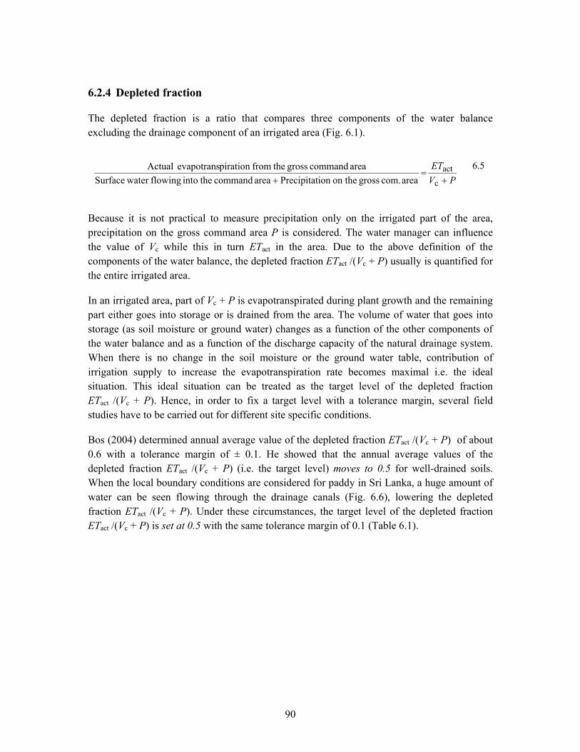
90

6.2.4 Depleted fraction

The depleted fraction is a ratio that compares three components of the water balance excluding the drainage component of an irrigated area (Fig. 6.1).

PVET

area com. gross on theion Precipitat area command theinto flowing water Surfacearea command gross thefrompiration evapotrans Actual

c

act+

=+

6.5

Because it is not practical to measure precipitation only on the irrigated part of the area, precipitation on the gross command area P is considered. The water manager can influence the value of Vc while this in turn ETact in the area. Due to the above definition of the components of the water balance, the depleted fraction ETact /(Vc + P) usually is quantified for the entire irrigated area.

In an irrigated area, part of Vc + P is evapotranspirated during plant growth and the remaining part either goes into storage or is drained from the area. The volume of water that goes into storage (as soil moisture or ground water) changes as a function of the other components of the water balance and as a function of the discharge capacity of the natural drainage system. When there is no change in the soil moisture or the ground water table, contribution of irrigation supply to increase the evapotranspiration rate becomes maximal i.e. the ideal situation. This ideal situation can be treated as the target level of the depleted fraction ETact /(Vc + P). Hence, in order to fix a target level with a tolerance margin, several field studies have to be carried out for different site specific conditions.

Bos (2004) determined annual average value of the depleted fraction ETact /(Vc + P) of about 0.6 with a tolerance margin of ± 0.1. He showed that the annual average values of the depleted fraction ETact /(Vc + P) (i.e. the target level) moves to 0.5 for well-drained soils. When the local boundary conditions are considered for paddy in Sri Lanka, a huge amount of water can be seen flowing through the drainage canals (Fig. 6.6), lowering the depleted fraction ETact /(Vc + P). Under these circumstances, the target level of the depleted fraction ETact /(Vc + P) is set at 0.5 with the same tolerance margin of 0.1 (Table 6.1).

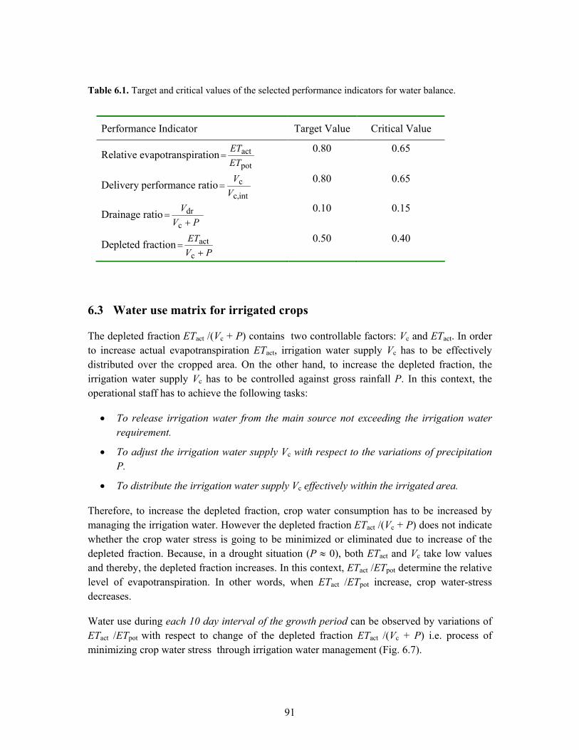
91

Table 6.1. Target and critical values of the selected performance indicators for water balance.

Performance Indicator Target Value Critical Value

Relative evapotranspirationpot

act ETET

= 0.80 0.65

Delivery performance ratiointc,

cV

V= 0.80 0.65

Drainage ratioPV

V c

dr+

= 0.10 0.15

Depleted fractionPV

ET

c

act+

= 0.50 0.40

6.3 Water use matrix for irrigated crops

The depleted fraction ETact /(Vc + P) contains two controllable factors: Vc and ETact. In order to increase actual evapotranspiration ETact, irrigation water supply Vc has to be effectively distributed over the cropped area. On the other hand, to increase the depleted fraction, the irrigation water supply Vc has to be controlled against gross rainfall P. In this context, the operational staff has to achieve the following tasks:

• To release irrigation water from the main source not exceeding the irrigation water requirement.

• To adjust the irrigation water supply Vc with respect to the variations of precipitation P.

• To distribute the irrigation water supply Vc effectively within the irrigated area.

Therefore, to increase the depleted fraction, crop water consumption has to be increased by managing the irrigation water. However the depleted fraction ETact /(Vc + P) does not indicate whether the crop water stress is going to be minimized or eliminated due to increase of the depleted fraction. Because, in a drought situation (P ≈ 0), both ETact and Vc take low values and thereby, the depleted fraction increases. In this context, ETact /ETpot determine the relative level of evapotranspiration. In other words, when ETact /ETpot increase, crop water-stress decreases.

Water use during each 10 day interval of the growth period can be observed by variations of ETact /ETpot with respect to change of the depleted fraction ETact /(Vc + P) i.e. process of minimizing crop water stress through irrigation water management (Fig. 6.7).

92

Figure 6.7 Water use matrix for irrigated crops showing performance of each 10 day interval over the growth period with four zones:

a) zone of Farmer satisfaction – crop water stress decreases by over supply of irrigation water b) zone of Water manager’s task - crop water stress decreases while utilizing minimum quantity of

irrigation water c) zone of Survival – crop growth affected by shortage of water d) zone of Risk – non-sustainable cultivation due to poor water management.

0.0

0.1

0.2

0.3

0.4

0.5

0.6

0.7

0.8

0.9

1.0

0.0 0.1 0.2 0.3 0.4 0.5 0.6 0.7 0.8 0.9 1.0Depleted fraction = ET act/(V c+P ) (-)

ET

act/E

Tpo

t (-)

Risk Survival

non-sustainable cultivation due to poor

water management

Crop growth affected by shortage of water

cd

Tran

sitio

nal r

ange

targ

et le

vel

criti

cal l

evel

Transitional range

target level

critical level

Farmer satisfaction Water manager's task

ba

Crop water consumption increases by managing irrigation water

Crop water consumption increases by over-supply

of irrigation water

Low

cro

p w

ater

stre

ssH

igh

crop

w

ater

stre

ss

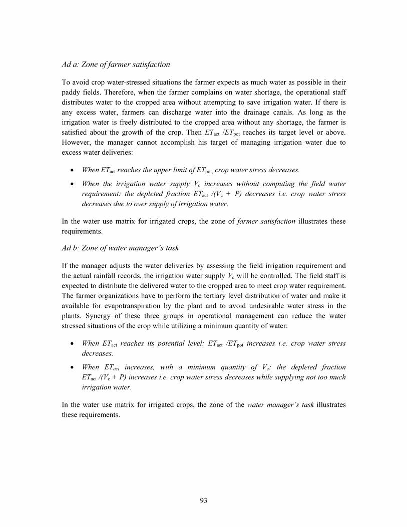
93

Ad a: Zone of farmer satisfaction

To avoid crop water-stressed situations the farmer expects as much water as possible in their paddy fields. Therefore, when the farmer complains on water shortage, the operational staff distributes water to the cropped area without attempting to save irrigation water. If there is any excess water, farmers can discharge water into the drainage canals. As long as the irrigation water is freely distributed to the cropped area without any shortage, the farmer is satisfied about the growth of the crop. Then ETact /ETpot reaches its target level or above. However, the manager cannot accomplish his target of managing irrigation water due to excess water deliveries:

• When ETact reaches the upper limit of ETpot, crop water stress decreases.

• When the irrigation water supply Vc increases without computing the field water requirement: the depleted fraction ETact /(Vc + P) decreases i.e. crop water stress decreases due to over supply of irrigation water.

In the water use matrix for irrigated crops, the zone of farmer satisfaction illustrates these requirements.

Ad b: Zone of water manager’s task

If the manager adjusts the water deliveries by assessing the field irrigation requirement and the actual rainfall records, the irrigation water supply Vc will be controlled. The field staff is expected to distribute the delivered water to the cropped area to meet crop water requirement. The farmer organizations have to perform the tertiary level distribution of water and make it available for evapotranspiration by the plant and to avoid undesirable water stress in the plants. Synergy of these three groups in operational management can reduce the water stressed situations of the crop while utilizing a minimum quantity of water:

• When ETact reaches its potential level: ETact /ETpot increases i.e. crop water stress decreases.

• When ETact increases, with a minimum quantity of Vc: the depleted fraction ETact /(Vc + P) increases i.e. crop water stress decreases while supplying not too much irrigation water.

In the water use matrix for irrigated crops, the zone of the water manager’s task illustrates these requirements.

94

Ad c: Zone of survival

Some cultivation seasons start with minimum storage in the irrigation reservoirs or minimum river flow in river-diversion schemes. In both cases, the monsoon rainfall is anticipated. If the anticipated rainfall does not occur during the cultivation, the manager has to limit water deliveries and yet save the crop. In such a situation, the available water has to be utilized more effectively:

• When water deliveries Vc are reduced during drought conditions (i.e. P≈ 0), ETact also reduces. In such a situation, the denominator (Vc + P) of the depleted fraction ETact /(Vc + P) dominates over the numerator ETact. Hence, the depleted fraction ETact /(Vc + P) increases

• When ETact decreases, ETact /ETpot also decreases affecting crop growth i.e. crop water stress exists due to lack of water available.

In the water use matrix for irrigated crops, the zone of survival illustrates these requirements i.e. the farmer can survive by saving the cultivation during a drought situation.

Ad c: Zone of risk

If in a drought situation as in the previous case, water is not effectively utilized, cultivation may fail. In addition, due to physical damages of the canal system (e.g. canal breaches, water leaks), more irrigation water flows into the drainage canals without being distributed in the cropped area. In such situations, both the depleted fraction ETact /(Vc + P) and the ETact /ETpot decreases i.e. crop water stress increases due to poor irrigation management. In the water use matrix for irrigated crops, the zone of risk illustrates these requirements i.e. the cultivation is not sustainable.

95

6.4 Performance assessment; examples of the Liyangastota scheme (right bank)

Performance of both parts of the Liyangastota scheme is assessed for three seasons. Here the results are given as an example for the right bank part of the scheme and one wet (2002-2003) and one dry (2003) season. Four indicators are used (Table 3.2): relative evapotranspiration ETact /ETpot, delivery performance ratio Vc /Vc,int, depleted fraction ETact /(Vc + P) and drainage ratio Vdr /(Vc + P). Concluding remarks are given at the end of this section.

6.4.1 Performance assessment for the wet season of 2002-2003.

The wet season of 2002-2003 started with land preparation on 18rd November 2002 and cultivation started in December (Fig. 6.8). Cultivation was delayed due to the ongoing rehabilitation program. Based on the graphical illustration of each performance indicator shown in Fig. 6.9, the operational performance of the scheme is assessed. The variation of ETact /ETpot versus the depleted fraction ETact /(Vc + P) for each interval is shown in the water use matrix for irrigated crops ( see Fig. 6.11).

The performance assessment is started with the relative evapotranspiration since it describes crop water stress against the potential water need. Throughout the season, ETact /ETpot fluctuated around its target value (Fig. 6.9a). The reasons for the shown performance levels can be diagnosed by assessing the water deliveries from the main source.

Figure 6.8 Cultivation calendar for the wet season of 2002-2003 of the Liyangastota right bank scheme.

0

12

Nov Dec Jan Feb Mar Apr

Initialstage

Developmentstage

Middlestage

Latestage

Irrigation water delivery period

Crop growth period

Ini_2Ini_1 Dev_1 Dev_2 Dev_3 Mid_1 Mid_2 Mid_3 Lat_1 Lat_2 Lat_3

Land preparation

96

Figure 6.9 Behaviour of the performance indicators during the wet season 2002-2003 at the Liyangastota right bank scheme: a) water use for crop growth, b) water deliveries and rainfall, c) drainage outflow, and d) water depletion. Note: *Excess water - subject to anticipated rainfall, more irrigation water has been delivered from the main source than required.

Good performanceTransitional range

Poor performance

0.40.50.60.70.80.91.0

Ini_

1

Ini_

2

Dev

_1

Dev

_2

Dev

_3

Mid

_1

Mid

_2

Mid

_3

Lat_

1

Interval

ET

act/E

Tpo

t (-)

target level

critical level

Good performance

Transitional range

Poor performance

0.0

0.5

1.0

1.5

2.0

Ini_

1

Ini_

2

Dev

_1

Dev

_2

Dev

_3

Mid

_1

Mid

_2

Mid

_3

Lat_

1Interval

Del

iver

y pe

rform

ance

ratio

= V

c/V

c,in

t(-)

0.01.53.04.5

6.07.59.0

Effe

ctiv

e ra

infa

ll -

Pe,

ant,

Pe

(mm

d-1

)

0.00.10.20.30.40.50.6

Ini_

1

Ini_

2

Dev

_1

Dev

_2

Dev

_3

Mid

_1

Mid

_2

Mid

_3

Lat_

1

Interval

Dra

inag

e ra

tio =

V

dr/(V

c+P

) (-)

critical level


High drainage flow

target level

target level

critical level

0.1

0.2

0.3

0.4

0.5

0.6

Ini_

1

Ini_

2

Dev

_1

Dev

_2

Dev

_3

Mid

_1

Mid

_2

Mid

_3

Lat_

1

Interval

Dep

lete

d fra

ctio

n =

E

Tac

t/(V

c+P

) (-)

critical level

target level

*Excess water

Poor performance

Transitional range

Good performance

(a)

(b)

(c)

(d)

P e,ant P e

97

In the beginning of the season, the delivery performance ratio Vc /Vc,int remained in the region of excess water (i.e. Vc /Vc,int = 1.5) and thereafter showed a decreasing trend. The command area has experienced less rainfall than anticipated. Throughout the season, the delivery performance ratio Vc /Vc,int is above its target level. This situation reveals that a short supply of irrigation water from the river diversion can no longer exist. There can be two possible reasons for the fluctuation of ETact /ETpot:

• A portion of delivered water has drained out from the canal system during the water deliveries.

• A portion of water retained in the cropped area has discharged to the drains.

During the initial stage and the beginning of the development stage, both the delivery performance ratio Vc /Vc,int and ETact /ETpot are kept above their target levels i.e. the manager has delivered more water from the reservoir than required and the cropped area has received sufficient water. Thus, the increasing trend of the drainage ratio Vdr /(Vc + P) during the initial stage indicates that excess water has drained from the cropped area.

In the field, when increased drainage flow is observed, the irrigation manager starts to reduce the water deliveries from the main source. Subsequently, the field staff also starts to reduce flow in the distributary system.

Throughout the season, rainfall has completely varied from its anticipated levels. Thus, for the field staff, manual operations of the canal system with frequent variations of rainfall would be rather complicated. However they have no real-time information on rainfall in order to make accurate adjustment in canal operations Hence, they perform canal operations based on their experience. Therefore, shortcomings in the field water distribution are unavoidable.

To retain water for a few days (i.e. 2 - 3 days) in the paddy fields, small bunds are formed in suitable intervals during land preparation (Fig. 6.10). Before the water level rises to the top of the field bunds, farmers divert excess water to the drainage canals. If the project area experiences regular rains when sufficient water is in the paddy fields, the farmer does not attempt to retain water in their paddy fields. Ultimately, the available water for the crop would decrease. In addition, because of moderately high permeability of the soil layers, it is not practical to retain water in the paddy fields for a longer period (i.e. more than 3 days). Under these circumstances, ETact/ETpot has fluctuated. The decreasing trend of evapotranspiration during the latter part of the season would seriously affect the grain yield than it did in the initial stages.

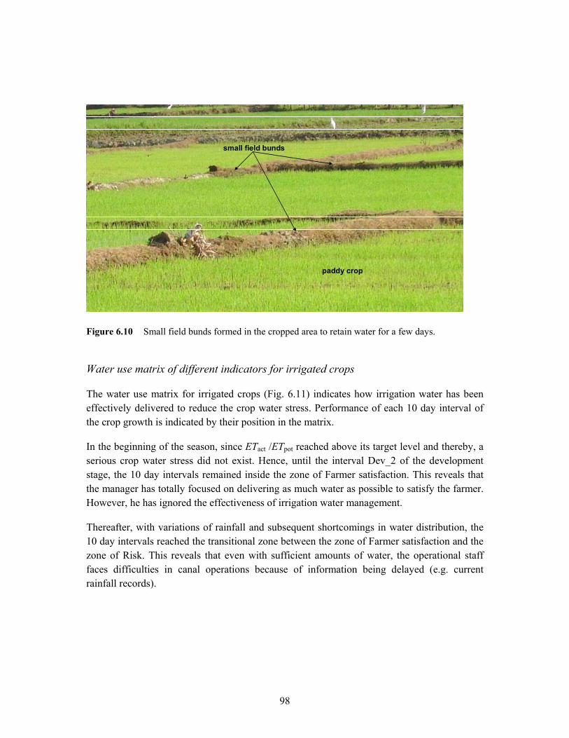
98

Figure 6.10 Small field bunds formed in the cropped area to retain water for a few days. Water use matrix of different indicators for irrigated crops

The water use matrix for irrigated crops (Fig. 6.11) indicates how irrigation water has been effectively delivered to reduce the crop water stress. Performance of each 10 day interval of the crop growth is indicated by their position in the matrix.

In the beginning of the season, since ETact /ETpot reached above its target level and thereby, a serious crop water stress did not exist. Hence, until the interval Dev_2 of the development stage, the 10 day intervals remained inside the zone of Farmer satisfaction. This reveals that the manager has totally focused on delivering as much water as possible to satisfy the farmer. However, he has ignored the effectiveness of irrigation water management.

Thereafter, with variations of rainfall and subsequent shortcomings in water distribution, the 10 day intervals reached the transitional zone between the zone of Farmer satisfaction and the zone of Risk. This reveals that even with sufficient amounts of water, the operational staff faces difficulties in canal operations because of information being delayed (e.g. current rainfall records).

small field bunds

paddy crop

small field bundssmall field bunds

paddy crop

99

During the entire season, the water deliveries have been increased without limiting to the actual requirement indicating over supply of irrigation water. In the irrigation schemes of Sri Lanka, the actual crop water deficit cannot be estimated because of non-availability of ETact measurements. As explained in section 2.4, in the near future, the Liyangastota scheme will receive less water from the Walawe river because of the new agricultural extension project in the Uda_Walawe left bank. Therefore it is necessary to use irrigation water in a productive manner.

Figure 6.11 Water use matrix for irrigated crops of the Liyangastota right bank scheme showing performance of each 10 day interval during the wet season 2002-2003 with four zones:



0.0

0.1

0.2

0.3

0.4

0.5

0.6

0.7

0.8

0.9

1.0


ET

act/E

Tpo

t (-)

Ini_1

Ini_2

Dev_1

Dev_2

Dev_3Mid_1

Mid_2

Mid_3

Lat_1

Risk Survival


water management


cd

Tran

sitio

nal r

ange

targ

et le

vel

criti

cal l

evel

Transitional range

target level

critical level


ba

100

6.4.2 Performance assessment for the dry season of 2003.

The dry season of 2003 started with land preparation on 27th April 2003 and cultivation started in June (Fig. 6.12). Based on the graphical illustration of each performance indicator shown in Fig. 6.13, the operational performance of the scheme is assessed. ETact estimated by remote sensing is shown in Fig. 6.14. The variation of ETact /ETpot versus the depleted fraction ETact /(Vc + P) for each interval is shown in the water use matrix for irrigated crops (see Fig. 6.15).

In this dry season both ETact /ETpot and the delivery performance ratio Vc /Vc,int are close to its target level with a few intermittent fluctuations. Until latter part of the development stage, ETact /ETpot is below its target level indicating that the cropped area has not received adequate water. This situation can be diagnosed by observing the other indicators.

In the beginning of the season, the delivery performance ratio Vc /Vc,int remains closely above its target level. The command area has received rainfall as anticipated. Thus, there cannot be a water shortage from the supply side. Hence, it is necessary to assess the performance of water distribution. The drainage ratio Vdr /(Vc + P) has increased above its critical level showing a portion of irrigation water has accumulated into the drainage canals. Justifying this situation, the depleted fraction ETact /(Vc + P) has moved below its critical level. This reveals that a substantial portion of the delivered water flowed directly into the drainage system. Since the water supply is on target, water cannot accumulate in the cropped area. Therefore, either the incorrect flow operations of the canal system or the physical damages of the canal system may cause the drain discharge to increase. When it rains, a substantial amount of rainfall runoff from the surrounding highlands accumulates in the drainage canals.

Figure 6.12 Cultivation calendar for the dry season of 2003 of the Liyangastota right bank scheme.

0

12

Apr May Jun Jul Aug Sep

Initialstage

Developmentstage

Middlestage

Latestage

Irrigation water delivery period

Crop growth period

Ini_2Ini_1 Dev_1 Dev_2 Dev_3 Mid_1 Mid_2 Mid_3 Lat_1 Lat_2 Lat_3

Land preparation

101

Figure 6.13 Behaviour of the performance indicators during the dry season 2003 at the Liyangastota right bank scheme: a) water use for crop growth, b) water deliveries and rainfall, c) drainage outflow, and d) water depletion. Note: *Excess water - subject to anticipated rainfall, more irrigation water has been delivered from the main source than required.

0.40.50.60.70.80.91.0

Ini_

1

Ini_

2

Dev

_1

Dev

_2

Dev

_3

Mid

_1

Mid

_2

Mid

_3

Lat_

1

Interval

ET

act/E

Tpo

t (-)

target level

critical level

Good performance

Transitional range

Poor performance

0.00.20.40.60.81.01.21.4

Ini_

1

Ini_

2

Dev

_1

Dev

_2

Dev

_3

Mid

_1

Mid

_2

Mid

_3

Lat_

1

Interval

Del

iver

y pe

rform

ance

ratio

= V

c/V

c,in

t (-)

0.00.51.01.52.02.53.03.54.0

Effe

ctiv

e ra

infa

ll -

Pe,

ant,

Pe

(mm

d-1

)

0.00.10.20.30.40.50.6

Ini_

1

Ini_

2

Dev

_1

Dev

_2

Dev

_3

Mid

_1

Mid

_2

Mid

_3

Lat_

1

Interval

Dra

inag

e ra

tio =

V

dr/(V

c+P

) (-)

critical level


High drainage flow

target level

target level

critical level

0.1

0.2

0.3

0.4

0.5

0.6

Ini_

1

Ini_

2

Dev

_1

Dev

_2

Dev

_3

Mid

_1

Mid

_2

Mid

_3

Lat_

1

Interval

Dep

lete

d fra

ctio

n =

E

Tac

t/(V

c+P

) (-)

critical level

target level


Poor performance

*Excess water

Poor performance

Transitional range

Good performance

(a)

(b)

(c)

(d)

P e,ant P e

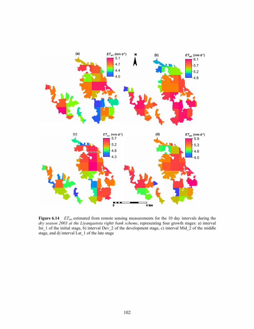
102

Figure 6.14 ETact estimated from remote sensing measurements for the 10 day intervals during the dry season 2003 at the Liyangastota rightt bank scheme, representing four growth stages: a) interval Ini_1 of the initial stage, b) interval Dev_2 of the development stage, c) interval Mid_2 of the middle stage, and d) interval Lat_1 of the late stage

5.9

5.3

4.6

4.0

5.7

5.2

4.8

4.3

6.1

5.7

5.2

4.8

5.1

4.7

4.4

4.0

(a) (b)

(c) (d)

N

0 16004 km0

ETact (mm d-1) ETact (mm d-1)

ETact (mm d-1)ETact (mm d-1)5.9

5.3

4.6

4.0

5.7

5.2

4.8

4.3

6.1

5.7

5.2

4.8

5.1

4.7

4.4

4.0

(a) (b)

(c) (d)

NN

0 16004 km00 16000 16004 km0

ETact (mm d-1) ETact (mm d-1)

ETact (mm d-1)ETact (mm d-1)

103

In the interval Mid_2, ETact /ETpot has suddenly dropped with variation of rainfall. However, ETact /ETpot has decreased to 0.7 and because of this, the plant would not go dry. Therefore, the farmers often do not complain about water. On the other hand, neither the farmers nor the field staff does have any measurements on ETact to check the crop water stress. In this dry season, ETpot increases due to dry weather condition with bright sun shine.

In order to get more water, some farmers block the canal flow and thereby the water level rises. A substantial amount of water overtops the canal bunds and flows into the drainage canals. However, it would be rather difficult to control, because all such malpractices are carried out during the night.

Water use matrix of different indicators for irrigated crops

In the beginning of the season, since ETact /ETpot reached marginally below its target level, the first four intervals (i.e. Ini_1 to Dev_2) positioned within the transitional range between the zone of Farmer satisfaction and the zone of Risk. Even with controlled condition, Fig. 6.13b illustrates that excess water deliveries from the main source. Thus, none of the positions of 10 day intervals in this dry season moved into the zone of Water manager’s task.

In the interval Mid_2, with a sudden drop of ETact /ETpot, its position has moved towards the zone of Risk. However, the next interval Mid_2 has moved sharply upward in the matrix. This indicates that in the latter case, the crop water stress has decreased. However, irrigation water management has therefore not improved. The manager has released irrigation water to meet the crop water requirement without attempting to save water.

Fig. 6.13b shows that in the intervals Dev_3, Mid_1, and Lat_1 of the season, the delivery performance ratio Vc /Vc,int as well as ETact /ETpot simultaneously reached their target levels. In the water use matrix, intervals have moved towards the zone of Water manager’s task while indicating reduced the crop water stress. During these intervals, the manager has responded the increased rainfall by reducing water deliveries. This reveals that the water productivity of the scheme could be further improved by controlling irrigation water supply and effective distribution of available water.

104

Figure 6.15 Water use matrix for irrigated crops of the Liyangastota right bank scheme showing performance of each 10 day interval during the dry season 2003 with four zones:



0.0

0.1

0.2

0.3

0.4

0.5

0.6

0.7

0.8

0.9

1.0


ET

act/E

Tpo

t (-)

Risk Survival


water management


cd Tran

sitio

nal r

ange

targ

et le

vel

criti

cal l

evel

Transitional range

target level

critical level


ba

Ini_1 Ini_2Dev_1

Dev_2Dev_3

Mid_2

Mid_3Lat_1

Mid_1

105

6.5 Concluding remarks

During the wet season, the manager has not followed the planned water delivery schedules and delivered more irrigation water than required. Hence, the water level in the paddy fields rises. Thus, a water deficit cannot exist in the cropped area. When rain starts, before the water level rises up to the field bunds, farmers drain excess water from the paddy fields. In this manner, rainwater also flows into the drainage canals. In reaction, the manager reduces water deliveries from the river diversion. Thus, ETact decreases. The drainage ratio Vdr /(Vc + P) also increases due to the defects of the canal system or incorrect canal operations. During the wet seasons, because of the over-supply of water, the delivery performance ratio Vc/Vc,int exceeds its target level.

With limited water availability, the dry season uses less irrigation water than the wet season. However, even in the dry season, the available water has not been used productively in the cropped area. Also, dry weather during dry season increases the potential evapotranspiration rate ETpot. In addition, due to malpractices of the farmers, the drainage ratio Vdr /(Vc + P) increases. Rainwater from surrounding highland areas also flows into the drainage canal system. Thus, the drainage ratio Vdr /(Vc + P) indicated values above its critical level.

When rainfall deviates from its anticipated level, the operational staff cannot make accurate adjustment in the water deliveries from the river diversion due to rainfall records being delayed. Such inaccurate adjustments would seriously affect the water distribution to the cropped area.

As shown in Fig. 6.16, the 10 day intervals in both seasons are distributed around the lower right corner of the zone of Farmer satisfaction. In the wet seasons, the operational staff has concentrated on distributing as much water as possible to the cropped area to satisfy the farmer. Therefore the crop water stress has decreased. However, in the wet season most of the 10 day intervals have remained within the zone of Farmer satisfaction. In the dry season, crop water stress has decreased even with available limited water and thereby, the 10 day intervals have shifted towards the zone of Water manager’s task.

The distribution of points in Fig. 6.16 are not scattered over the water use matrix. This reveals that the operational staff has succeeded to control the scheme performance without allowing it to perform in the danger zones i.e. the zones of Risk or Survival. However, to reach the zone of Water manager’s task, the operational performance should be further improved, which is the ultimate goal.

106

Figure 6.16 Water use matrix for irrigated crops of the Liyangastota right bank scheme showing performance of each 10 day intervals during the wet season 2002-2003 and the dry season 2003:



In order to accomplish the ultimate goal, the operational staff needs to deviate from their routine practices or rule based approach: when it rains heavily, they reduce water deliveries from the main source without any quantification and lift flow control gates for the safety of the canal system: when there is no rain or less rain as they feel, they increase irrigation water supply to stop farmer complains. They have to adopt a situational approach i.e. planning, monitoring, and assessing irrigation performance to diagnose the situation and thus to take corrective measures: performance oriented water management strategy.

0.0

0.1

0.2

0.3

0.4

0.5

0.6

0.7

0.8

0.9

1.0


ET

act/E

Tpo

t (-)

Risk Survival


water management


cd Tran

sitio

nal r

ange

targ

et le

vel

criti

cal l

evel

Transitional range

target level

critical level


ba

wet seasondry season

107

A period of 4-5 d is applied for the rotational water issues in paddy cultivation of the dry zone. When a water problem is identified, rotational water issues are started within the problematic area as a remedy. Thus, time delays can be minimized. Thereafter, system adjustments will be started from the down stream to the upstream. If necessary more water is release from the main source. With the available rate of suitable satellite images (25 – 35 images per growing period of 90 days), these performance indicators can be updated within 4 – 5 day intervals. Therefore, it is practically possible to assess the irrigation performance associated with MODIS images as a decision supportive tool.

It is necessary to establish a more realistic crop-water production function for paddy in Sri Lanka by considering its growth related factors such as crop variety, seasonal weather condition etc. As a paddy grown country, research fields are available for such studies. Also to study the ground water recharge, specific studies have not been reported in the research field of the irrigated agriculture. Such research findings are needed to establish the target and critical levels of the depleted fraction under the local boundary conditions. These two research studies are very much useful to improve the results of this study.

109

7. Assessing socio-economic performance and institutional arrangements

7.1 Introduction

In irrigated agriculture, socio-economic performance is used to assess strategic decisions related to different management levels as specified in the management hierarchy of Fig. 3.1. As shown in Fig. 3.4 socio-economic interactions on one hand occur between the Government and the water institution, on the other hand between Government and the farmer organizations.

Socio-economic performance is assessed for the Left bank and the Right bank of the Uda_Walawe scheme, and the Left bank and the Right bank of the Liyangastota scheme. The three consecutive seasons starting from October 2002 to April 2004 are considered for the assessment. As shown in Table 3.2, the indicators used to assess the socio-economic performance of each sub-scheme are seasonal grain yield Yact, water productivity WPm,ET, and the price ratio Rprice. The grain yield Yact and the water productivity WPm,ET were computed from data acquired through remote sensing.

7.2 Seasonal grain yield

The grain yield Yact at the end of the season is defined as the seasonal harvest of paddy grain by mass in terms of the cultivated land area (e.g. kg ha-1), which is given in Eq.7.1.

crop

grain area Cropped

production Crop A

m=

7.1

The farmer needs to recover the investment made on paddy cultivation and to improve his living standard from the seasonal harvest. With increasing costs of input commodities such as fertilizer, pesticides, labor, machinery, seed paddy etc, farmer can survive only by increasing grain yield.

The target value and critical value of the grain yield Yact have been already determined (see Fig. 6.5) as 5 ton ha-1 (i.e. 5000 kg ha-1) and 4 ton ha-1 respectively. The Yact estimated by remote sensing are shown in Figures 7.1 – 7.2 and tabulated in Table 7.1.

110

Figure 7.1 Grain yield estimated from remote sensing measurements for the dry season 2003 at the Uda_Walawe right bank scheme.

5697

4898

4099

3300

Seasonal grain yield Yact (kg ha-1)

N

0 16008 km0

5697

4898

4099

3300


NN

0 16008 km00 16000 16008 km0

111

Figure 7.2 Grain yield estimated from remote sensing measurements for the dry season 2003: a) at the Uda_Walawe left bank scheme, b) at the Liyangastota right bank scheme, and c) at the Liyangastota left bank scheme.

5508

4900

4292

3684


5122

4564

4007

3449


5692

4800

3909

3017


N

0 160008 km0

(a)

(b) (c)

5508

4900

4292

3684


5122

4564

4007

3449


5692

4800

3909

3017


NN

0 160000 160008 km0

(a)

(b) (c)

112

Table 7.1 Grain yield Yact derived by remote sensing at the end of three seasons for the four sub-schemes.

Seasonal grain yield Yact Sub-scheme

2002-2003 wet season

kg ha-1

2003 dry season

kg ha-1


kg ha-1

Liyangastota left bank 4702 4495 5012

Liyangastota right bank 4646 4290 4843

Uda_Walawe left bank 4860 4609 4746

Uda_Walawe right bank 5010 4702 4854

The grain yields shown in Table 7.1 are above the critical level of 4000 kg ha-1. In two occasions (i.e. 2002-2003 of the Uda_Walawe right bank and 2003-2004 of the Liyangastota left bank) the grain yield Yact reached its target level. The wet season of 2003-2004 has higher grain yields Yact than the other two seasons. The dry season 2003 has the lowest values.

The operational managers in the management hierarchy can be satisfied with the seasonal grain yield Yact, as it reached above critical level without launching any yield improvement program. This reveals that the present grain yield could be further improved by introducing such a program.

The grain yields of Table 7.1 are close to each other. Under the Liyangastota scheme, paddy cultivation has been carried out for more than 100 years and for the Uda_Walawe scheme for 30 years. In Sri Lanka, irrigated paddy cultivation has a long history of more than 2000 years. Thus, unless a drought situation exists, with routine water management practices of the field staff, and the traditional cultivation practices of the farmers, grain yield Yact rarely shows irregular fluctuations. In this context, also the similarities between the schemes such as soils, weather, water availability, variety of paddy can be considered. Hence, the field staff and the farmers have managed to maintain the grain yield Yact at a uniform level, being above the critical level.

7.2.1 Comparison of grain yield with field measurements

The grain yield as estimated by remote sensing can be compared with data collected through crop cutting surveys. The Department of Census and Statistics of Sri Lanka collects sample data on the basis of irrigation schemes (i.e. the Liyangastota scheme and the Uda_Walawe scheme). Hence, for the comparison of results, the yields derived from remote sensing were converted from the sub-scheme level to the scheme level by averaging (Table 7.2).

113

Table 7.2 shows that grain yield estimated by the Census and Statistics Department deviates from the remote sensing outputs within a range of - 4.5% to + 4.9%. The sample data collection through crop cutting surveys starts at the end of the season. Such surveys have to be completed within a very short period remains for harvesting (say about 2-3 weeks) because of the forthcoming inter monsoon rains. In addition, to collect crop cutting data, a limited number of field officers are employed in each district. These restrictions limit the number of samples, which could be collected. This manual process takes more than 4 weeks. If there is a shortage of paddy, without timely information on the seasonal harvest, it is difficult for the Government to plan for a national import program. Several occasions during past years (say 10 years), the Government (the decision maker) faced this difficulty. However, grain yield can be estimated using satellite remote sensing just before the start of crop cutting. Hence, it provides grain yield information to the decision makers with a minimum time gain of 4 weeks and such information is human unbiased. Due to the low resolution of the pixels such as MODIS, grain yield estimation needs the command area to be at least 2000 ha (as explained under section 5.3.4).

Table 7.2 Grain yield Yact of the Liyangastota scheme and the Uda_Walawe scheme derived from remote sensing as well as crop cutting surveys based on the schemes.*Source: Seasonal paddy production, the Department of Census and Statistics, Sri Lanka (2002-2004).

Seasonal crop yield Yact Scheme

Data from remotesensing

kg ha-1

Data from the Department of Census and Statistics

kg ha-1

Deviation of remote sensing data as a % of statistical data

2002-2003 wet season Liyangastota 4674 4897 4.6 Uda_Walawe 4935 5192 4.9

2003 dry season Liyangastota 4393 4205 -4.5 Uda_Walawe 4656 4872 4.4

2003-2004 wet season Liyangastota 4929 5165 4.6 Uda_Walawe 4801 5044 4.8

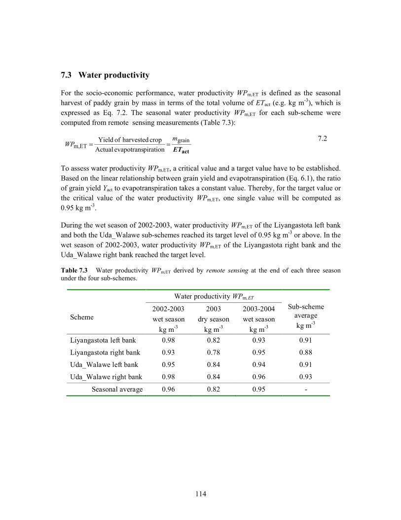
114

7.3 Water productivity

For the socio-economic performance, water productivity WPm,ET is defined as the seasonal harvest of paddy grain by mass in terms of the total volume of ETact (e.g. kg m-3), which is expressed as Eq. 7.2. The seasonal water productivity WPm,ET for each sub-scheme were computed from remote sensing measurements (Table 7.3):

actETgrain

ETm, pirationevapotrans Actual

crop harvested of Yield m

WP == 7.2

To assess water productivity WPm,ET, a critical value and a target value have to be established. Based on the linear relationship between grain yield and evapotranspiration (Eq. 6.1), the ratio of grain yield Yact to evapotranspiration takes a constant value. Thereby, for the target value or the critical value of the water productivity WPm,ET, one single value will be computed as 0.95 kg m-3.

During the wet season of 2002-2003, water productivity WPm,ET of the Liyangastota left bank and both the Uda_Walawe sub-schemes reached its target level of 0.95 kg m-3 or above. In the wet season of 2002-2003, water productivity WPm,ET of the Liyangastota right bank and the Uda_Walawe right bank reached the target level.

Table 7.3 Water productivity WPm,ET derived by remote sensing at the end of each three season under the four sub-schemes.

Water productivity WPm,ET Scheme


kg m-3

2003 dry season

kg m-3


kg m-3

Sub-scheme

average kg m-3

Liyangastota left bank 0.98 0.82 0.93 0.91

Liyangastota right bank 0.93 0.78 0.95 0.88

Uda_Walawe left bank 0.95 0.84 0.94 0.91

Uda_Walawe right bank 0.98 0.84 0.96 0.93

Seasonal average 0.96 0.82 0.95 -

115

During the dry season of 2003, WPm,ET of all four sub-schemes is below target level. Because of this, WPm,ET of all four sub-schemes during the entire study period (from the wet season of 2002-2003 to the wet season of 2003-2004) has not reached the target level.

During dry seasons more water evaporates from the paddy fields than in wet seasons. In addition, grain yield Yact in the dry season of 2003 is less than the two wet seasons. Thus, WPm,ET of the dry season of 2003 is relatively low.

Presently, the seasonal WPm,ET is not estimated because of non-availability of ETact measurements. As shown in Table 1.2, the total irrigation water supply from the main source is determined in terms of irrigated area (e.g. m3 ha-1).

Both performance indicators, the grain yield Yact and WPm,ET determine the total mass of harvested grain mgrain at the end of the season. Therefore, variations of these two indicators can be observed (Fig. 7.3).

Figure 7.3 Behaviour of the water productivity WPm,ET versus the grain yield Yact for each three season of the four sub-schemes in the study area.

0.0

0.1

0.2

0.3

0.4

0.5

0.6

0.7

0.8

0.9

1.0

1.1

1.2

0 500 1000 1500 2000 2500 3000 3500 4000 4500 5000 5500

Grain yield, Y act (kg ha-1)

Wat

er p

rodu

ctiv

ity, W

Pm

,ET (k

g m

-3) target level

targ

et le

vel

criti

cal l

evel

116

As shown in Fig. 7.3, in some seasons the WPm,ET is above its target level; but Yact remains below its target level. Most seasons may do not have access to find high quality seed paddy. As the Agriculture Department cannot supply the total demand of high yielding seed paddy, they recommend farmers to retain good quality paddy from their seasonal cultivation to use as seed paddy. There is no program to verify the quality of seed paddy produced by the farmers. Yact of such low quality seeds does not reach its target level even with increased ETact. In addition, how the farmer care about the crop throughout the season is also important to increase Yact. As explain in section 2.5 farmers engage other income generating activities for their survival until they harvest i.e. quality of the farmer.

7.3.1 Comparison of water productivity of paddy with published studies

Seasonal values of WPm,ET were computed based on 10 day MODIS data for each scheme (Appendix D). The range of minimum values and the range of maximum values were obtained as 0.37 – 0.68 kg m-3 and 1.06 – 1.24 kg m-3. Presently, the seasonal WPm,ET is not estimated because of non-availability of ETact measurements. For the comparison, maximum and minimum values obtained from a literature review were used (Fig. 7.4).

Figure 7.4 Comparison of the water productivity WPm,ET estimated from remote sensing for this study with WPm,ET for paddy in published studies.

In this study

Doorenbos and Kassam (1979)

Toung and Bouman (2003)

Zwart and Bastiaanssen (2004)

02468

1012141618

0 0.1 0.2 0.3 0.4 0.5 0.6 0.7 0.8 0.9 1 1.1 1.2 1.3 1.4 1.5 1.6 1.7

Water productivity WP m, ET (kg m-3)

min. max.

min. max. 0.37 0.68 1.06 1.24

1.1

min. max.

1.60.6

max.min.

0.4 1.6

0.7

117

Fig. 7.4 shows that the minimum range of the WPm,ET is close to the minimum values obtained from the other studies. The maximum WPm,ET of this study and the maximum value mentioned by Doorenbos and Kassam, (1979) are compatible. However, in paddy production WPm,ET increased through the years due to developments in new high yielding plant types with a higher ratio of photosynthesis to transpiration (Peng et al., 1998; Tong, 1999). The maximum values go up to 2.20 kg m-3 and were measured in China on alternate wetting and drying paddy plots (Dong et al., 2001) with highest rice yields of over 10000 kg ha-1. Also in the study area, certain high yielding paddy varieties have been introduced to suit the local conditions. However, the water productivity WPm,ET did not exceed 1.24 kg m-3 as indicated above. The same reasons given in the section 7.2.1 can be used to explain the situation which can be summarized as follows.

• The availability of improved seed varieties is not sufficient to fulfill the farmer’s demand.

• There is no program to maintain and verify the quality of seed paddy reproduced by the farmers.

• Farmer’s give little attention to the crop throughout the cultivation.

The behaviour of the seasonal grain yield Yact against the seasonal ETact (mm season-1) is shown in Fig. 7.5. Since the dry season 2003 indicated low WPm,ET, the dry season and the wet seasons are shown separately. The number of data points is not sufficient to assess the correlation between Yact versus ETact. However, a comparison can be made among Yact, WPm,ET and the delivery performance ratio Vc /Vc,int with following conclusions.

• During the dry season, greater slope of Yact versus ETact (Fig. 7.5) is shown than in the wet season. This determines that in the dry season, the consumptive use of water produces grain higher than in the wet season. However, during the wet season, WPm,ET relatively increases.

• Table 7.2 has shown that during the wet seasons, farmer produces more grain per unit land area than in the dry season. Hence, during the wet season, Yact relatively increases.

• The delivery performance ratio (Vc /Vc,int) for the wet season (Figures 6.9) shows excessive high values. For the dry season Figure 6.13 shows near-target values of the ratio while values of ETact / ETpot are the same order of magnitude. This indicates that Vc can be reduced during the wet season.

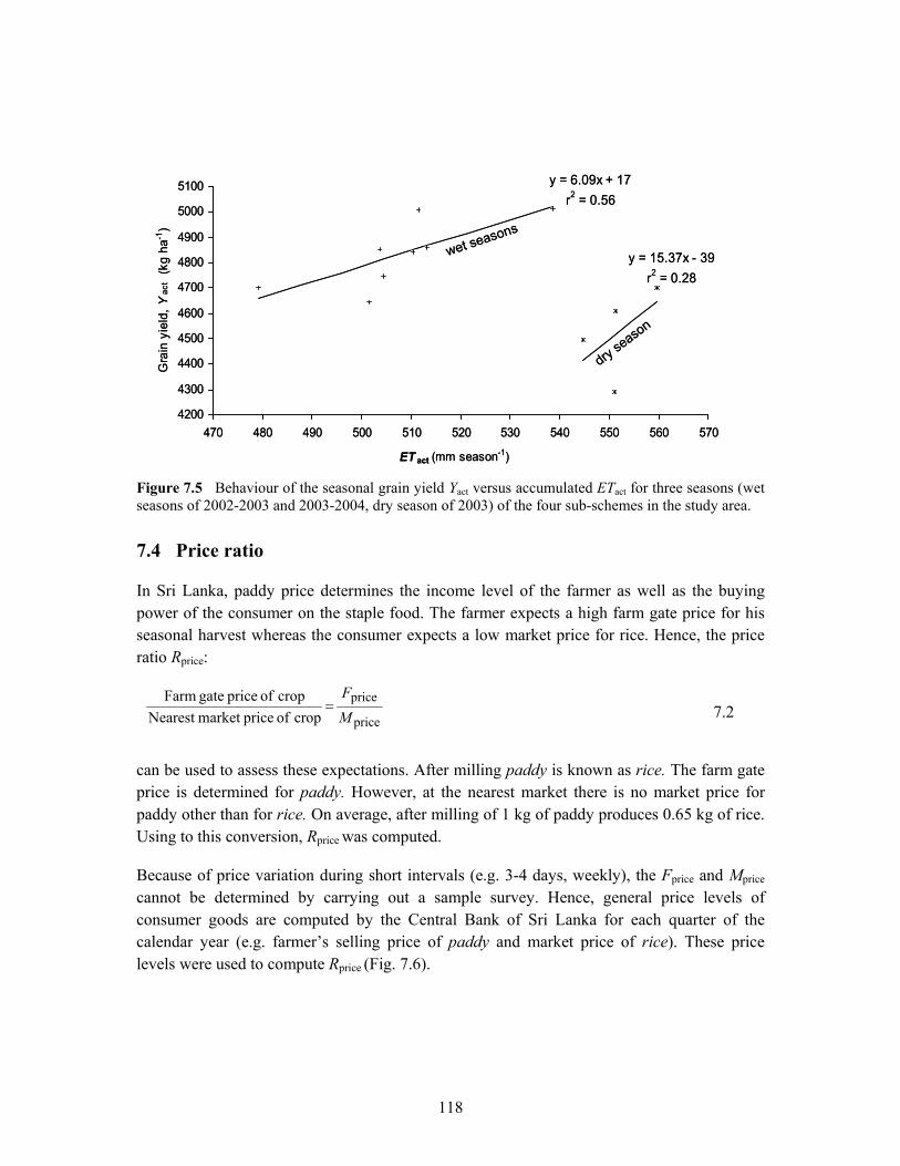
118

Figure 7.5 Behaviour of the seasonal grain yield Yact versus accumulated ETact for three seasons (wet seasons of 2002-2003 and 2003-2004, dry season of 2003) of the four sub-schemes in the study area.

7.4 Price ratio

In Sri Lanka, paddy price determines the income level of the farmer as well as the buying power of the consumer on the staple food. The farmer expects a high farm gate price for his seasonal harvest whereas the consumer expects a low market price for rice. Hence, the price ratio Rprice:

price

price crop of pricemarket Nearest

crop of price gate FarmMF

=

7.2

can be used to assess these expectations. After milling paddy is known as rice. The farm gate price is determined for paddy. However, at the nearest market there is no market price for paddy other than for rice. On average, after milling of 1 kg of paddy produces 0.65 kg of rice. Using to this conversion, Rprice was computed.

Because of price variation during short intervals (e.g. 3-4 days, weekly), the Fprice and Mprice cannot be determined by carrying out a sample survey. Hence, general price levels of consumer goods are computed by the Central Bank of Sri Lanka for each quarter of the calendar year (e.g. farmer’s selling price of paddy and market price of rice). These price levels were used to compute Rprice (Fig. 7.6).

wet seasons

dry season

y = 6.09x + 17r2 = 0.56

y = 15.37x - 39r2 = 0.28

4200

4300

4400

4500

4600

4700

4800

4900

5000

5100

470 480 490 500 510 520 530 540 550 560 570

ET act (mm season-1)

Gra

in y

ield

, Yac

t (k

g ha

-1)

wet seasons

dry season

y = 6.09x + 17r2 = 0.56

y = 15.37x - 39r2 = 0.28

4200

4300

4400

4500

4600

4700

4800

4900

5000

5100

470 480 490 500 510 520 530 540 550 560 570

ET act (mm season-1)

Gra

in y

ield

, Yac

t (k

g ha

-1)

119

Figure 7.6 Variation Rprice of a paddy crop from 2000 to 2004. Source: Monthly bulletin, Central Bank of Sri Lanka (2002 - 2005).

Fig. 7.6 indicates that the Rprice is rather stable around 0.78. When the country reaches near self-sufficiency in paddy production, the Mprice will be stable against the consumer demand and the farmer gets a stable price for the product Fprice. In the short run, a stable Rprice provides benefits to the farmer as well as to the consumer. In the long run, the escalating cost of production of paddy would lower the investment power of the farmer on paddy cultivation. To compensate for this trend, the Government frequently offers the farmer a price increase of paddy.

If there is a production shortage of paddy, without timely information on the seasonal harvest, it is difficult for the Government to plan for a national import program because of delays in crop cutting surveys. All records are manually entered and it takes a long time to compile and transform data into a digital database. In addition to this time lag, the import process itself takes at least two months. When the market receives the imported rice, the farmer would get ready to harvest his next crop. Thus, producer prices of paddy would fall, which would lower the income level of the paddy farmer. This reveals that the marketing of paddy is a highly time depended activity. However, grain yield estimation using satellite remote sensing can reduce the time taken for sampling. Thereby, the Government can take the decision before 3 – 4 weeks ahead.

0.0

0.1

0.2

0.3

0.4

0.5

0.6

0.7

0.8

0.9

1.0

1st Q

tr

2nd

Qtr

3rd

Qtr

4th

Qtr

1st Q

tr

2nd

Qtr

3rd

Qtr

4th

Qtr

1st Q

tr

2nd

Qtr

3rd

Qtr

4th

Qtr

1st Q

tr

2nd

Qtr

3rd

Qtr

4th

Qtr

1st Q

tr

2nd

Qtr

3rd

Qtr

4th

Qtr

Pric

e ra

tio, R

pric

e (-)

2000 2001 2002 2003 2004

average price ratio = 0.78

120

7.5 Recommended Institutional arrangements for the Irrigation Department

During the entire assessment process, it indicated the importance of timely observations to assess the performance, to diagnose the situation, and to find the root cause for performance gap (if any). However, to achieve the strategic objectives in the irrigation sector (e.g. to increase the grain yield Yact by minimum utilization of input resources), the operational performance as well as the socio-economic performance of irrigation schemes have to be improved.

As irrigation water is distributed free of charge, the farmer expects as much water as possible. However, with the development of the new command area in the Uda_Walawe left bank, the existing command area will be increased by 25% and thereby, irrigation water will become limited.

In this process, near real-time data of both point measurements and area measurements are required. The delivery performance ratio Vc /Vc,int can be assessed by the measurements of flow measuring structures. However, from the operational performance it was observed that the field staff as well as the manager did not give due attention to the drainage component of the water balance. In situations where the water delivery performance shows a decreasing trend even with adequate irrigation water supply, the drainage ratio Vdr /(Vc + P) can be used to diagnose the main causes. Hence, the drainage measurements in the secondary and the tertiary units of the scheme are recommended. To determine the crop water requirement, near real-time ETact is required. With low cost satellite measurements such as MODIS, ETact, can be estimated. In addition, when it is raining in the project area current rainfall records are necessary to adjust the canal flow. Low-cost mobile weather stations (digital) are now available (e.g. 3000 US $). It is recommended to install such systems within the command area of large irrigation schemes (based on the extent) to obtain real-time weather data such as, rainfall intensity, wind speed, air temperature. Such systems provide data based on short time intervals.

Under these circumstances, performance assessment of the irrigation schemes is recommended in the Irrigation Department (as one of the key stakeholders). The author of this thesis recommends to implement the following strategies.

• Introduce a performance assessment program for the irrigation schemes, with a minimum number of indicators as used in this study.

• Arrange obtaining near real-time measurements of rain fall from digital weather stations, ETact from low cost satellite data and canal flows from regular field measurements.

121

• Carry out GIS operations and satellite remote sensing for estimating ETact through the SEBAL approach and thereby, for quantifying related parameters of the selected performance indicators.

• Select and train staff for image processing, GIS techniques, and data processing related to performance evaluations i.e. to implement the proposed program.

• Cooperate with farmer organizations to achieve the objectives of the performance assessment program.

In order to implement a performance evaluation program as above, a central monitoring unit for each irrigation scheme should be established (Fig. 7.7).

Figure 7.7 Organizational setup to implement a performance assessment program in the Irrigation Department of Sri Lanka.

Irrigation Department

Irrigation management branch

Geoinformaticsbranch

Training program on geoinformatics

Remote sensing measurements

Divisional Irrigation Engineer

(Irrigation manager)

Field staff Office staff

Monitoring and performance assessment unit

Near real-time information

Regular field measurements

Rainfall records and weather data

Irrigation Department

Irrigation management branch

Geoinformaticsbranch

Training program on geoinformatics

Remote sensing measurements

Divisional Irrigation Engineer

(Irrigation manager)

Field staff Office staff

Monitoring and performance assessment unit

Near real-time information

Regular field measurements

Rainfall records and weather data

122

The recently established branch for Geoinformatics in the Irrigation Department should carry out such training programs with the cooperation of the Irrigation Management branch. It is recommended to start the performance assessment program with a few irrigation schemes (e.g. two or three schemes located close by). With that experience and skills, the program can be rapidly developed into the other irrigation schemes.

In the large and medium irrigation schemes in Sri Lanka, tertiary level water distribution is carried out by the farmer organizations. At present, the field staff delivers the irrigation water up to the tertiary level canal system and thereafter the farmer organizations distribute water to the paddy fields. Hence, to improve the irrigation performance, the farmer organizations as well as the field staff have to co-operate. The present exercise of minimizing water stress condition in the cropped area by increasing water deliveries should no longer exist. A new task of increasing of seasonal grain yield Yact by improving water productivity WPm,ET is recommended to put into practice.

123

Summary and conclusions Problem statement

The present challenge for irrigated agriculture is to improve food security through more efficient and effective use of water. Paddy, as the staple food crop, is widespread in Sri Lanka. The consumptive use of water by crops ETact is only part of the total irrigation water supply from a river diversion or a reservoir.

In Sri Lanka, most of the irrigation schemes are located in the dry zone and therefore, water use for irrigated agriculture is a critical issue. The national annual average yield of rice is around 50 % of the genetic potential of improved cultivars. This yield gap has to be reduced by improving productivity of paddy cultivation. The rationale behind performance assessment is to diagnose the performance and to rectify the shortcomings. Therefore, a suitable performance assessment program has to be developed. In Sri Lanka, paddy farmers have an income below the poverty line. To correct this, paddy cultivation is subsidized by the government, e.g. irrigation water is delivered free of charge. Therefore, to improve performance of irrigation schemes, a heavy cost incurring program is not viable.

To assess irrigation performance, objective data on actual field performance are needed. The improved facilities of satellite remote sensing can now provide information on a daily basis of biomass, of soil moisture and of ETact with spatial resolutions of 250 m to 1000 m.

Because the growth duration of paddy varieties varies from 105 to 120 days, field conditions need to be monitored in intervals of at least 10 days. The MODIS (MODerate resolution Imaging Spectroradiometer) images with one day temporal resolution can provide data within the required monitoring frequency even allowing for some cloudy days. In addition, these images are freely available through the internet, the only cost being that of downloading them. The MODIS images with 1000 m × 1000 m spatial resolution were selected for the present study. This study however, assesses mainly whether satellite measurements are sufficiently accurate to support management decisions.

The main objective of this study was to develop and introduce a cost effective performance assessment program to manage irrigation systems using satellite remote sensing as a tool, and to assess whether the results are sufficiently accurate to support the managerial decisions at all levels.

124

Study area

The study area consists of the Uda_Walawe and the Liyangastota irrigation schemes. They are located in the South-east dry zone of Sri Lanka (Fig. 2.1). Each scheme has two sub-schemes: one is at the right bank and the other one at the left bank. They provide irrigation facilities for about 20000 ha of paddy. The annual rainfall in the study area fluctuates around 1000 mm.

Performance assessment program

Chapter 3 discusses the needs of key stakeholders and the boundary conditions to assess the irrigation performance of paddy cultivation. Distinctions and interrelation between strategic performance and operational performance were elaborated. In this thesis, a new rational approach was proposed to select appropriate performance indicators. The key stakeholders of irrigated agriculture were identified as the Government, the Irrigation Department, and the Farmer Organizations. The interaction between key stakeholders determines how they are accountable to one another in terms of irrigated agriculture: water balance, socio-economics, and environmental constraints. To assess operational performance and socio-economic performance, the selected indicators quantify water use and grain yield production.

Satellite remote sensing approach to determine crop parameters

Actual evapotranspiration ETact is one of the water balance components used to assess the performance of irrigated crops. Presently, in Sri Lanka, field measurements of ETact are not available. Chapter 4 presents the Surface Energy Balance Algorithm for Land (SEBAL) approach for computing ETact over the cropped area using MODIS images. The SEBAL approach requires a limited number of weather data which are available at the Meteorology Department of Sri Lanka. Potential evapotranspiration ETpot was estimated through the Penman-Monteith approach. In addition, above canopy net-radiation derived from remote sensing measurements were also incorporated. A remote sensing model applying reflectance data was used to estimate the seasonal grain yield prior to start harvesting.

Accuracy assessment of information from the MODIS images

In chapter 5, the ETact -error due to the spatial scale of the MODIS images was described as the deviation of ETact with respect to those derived from the Landsat data.

The input parameters of the MODIS and the Landsat data represent two distinctive pixel sizes of 1000 m and 30 m respectively. Hence, the smaller pixels of Landsat were transformed into the size of the larger pixel of MODIS by incorporating the neighbouring pixels through a linear aggregation by 33 × 33 pixels. Some of the model functions of the SEBAL approach (e.g. Normalized Difference Vegetation Index - NDVI) were formulated by non-linear relationships among input variables. Therefore, linear aggregation of pixels was followed by the SEBAL approach.

125

Spectral properties over the ground may be varying due to the heterogeneity of vegetation cover. Therefore, a normal distribution of spectral measurement values cannot be assumed for each sample of 33 × 33 set of pixels. For a comparison, computation of ETact was carried out by taking the mean value, the median value and the mode value of the sample aggregation. The results indicate that ETact values computed by taking mean values have the highest correlation with the corresponding ETact values derived from the MODIS data. Under water stressed situations, the ETact derived from the 1000 m × 1000 m MODIS data deviated 10% from those derived from the 30 m × 30 m Landsat data. However, under normal situations (i.e. ETact being close to ETpot), this deviation was reduced to only 6% and below.

The error component of ETact when ground cover area increases could be described as follows:

Case 1: When the area concerned was too small as compared with the low resolution of the MODIS measurements, the impact of boundary pixels on the final output value would be significant.

Case 2: When the area concerned was too large compared with the heterogeneity of the land cover (i.e. site specific condition), the effect due to the variations of the pixel values would dominate the final output.

Firstly, the error component of ETact was estimated for a sample of 4 × 4 pixels in a MODIS output map of SEBAL. To make an unbiased representation, a large extent of the cloud free area was selected, the population being represented by 324 samples. Linear regression analysis was applied for error estimation. Using the same SEBAL output map of ETact, the sample size was increased from 4 × 4 pixels to 12 × 12 pixels by discrete intervals within the same population. Secondly, the same process was within a cultivation season repeated for three data sets representing the initial, development, and middle growth stages.

If the spatial extent of the land cover was less than 2000 ha, the error increased (Case 1). If the spatial extent was greater than 4000 ha, the error increased (Case 2). The upper limit of 4000 ha is very site specific and depends on the variation of ground cover over the area concerned. In Sri Lanka, an irrigation scheme having a command area of 400 ha is even treated as a large irrigation scheme. Hence, to determine ETact under the prevailing local boundary conditions, the spatial extent between Case 1 and Case 2 is recommended as more suitable for the MODIS measurements.

Assessing strategic irrigation performance

In chapter 6, two examples of assessing operational irrigation performance were given: one for the Liyangastota right bank during the wet season of 2002-2003, the second for the same scheme during the dry season of 2003. The temporal scale for each growth stage was

126

considered to begin with 10 day intervals. The indicators used were: relative evapotranspiration ETact /ETpot, delivery performance ratio Vc /Vc,int, depleted fraction ETact /(Vc + P) and drainage ratio Vdr /(Vc + P). To assess the irrigation performance, the target levels and the critical levels of each performance indicator was established by considering the present irrigation practices and the attainable targets stipulated for the paddy cultivation (see Table 6.1).

During the wet and dry seasons, ETact fluctuated around 80 % of its potential value. During the wet season, the irrigation managers delivered more irrigation water than required. Due to these excess water deliveries as well as rainwater from surrounding highland areas which also flows into the drainage canal system, the drainage ratio Vdr /(Vc + P) increased. With limited water availability over the dry season less irrigation water was used than over the wet season. However, even in the dry season, the available water was not used productively.

In addition, by combining two indicators, i.e. relative evapotranspiration ETact /ETpot and depleted fraction ETact /(Vc + P), a new water use matrix for irrigated crops was introduced in this thesis. The matrix describes how effectively the irrigation manager has delivered the irrigation water to reduce crop water stress. Based on this matrix, each 10 day interval of the growth period is positioned in each of the following four zones (see Fig.6.7).

a) Zone of Farmer satisfaction – crop water stress decreases by over supply of irrigation water.

b) Zone of Water manager’s task - crop water stress decreases while using minimum quantity of irrigation water.

c) Zone of Survival – crop growth reduced by shortage of water.

d) Zone of Risk – non-sustainable cultivation due to poor water management.

Evaluations by the water use matrix indicated that the 10 day intervals in both seasons were positioned around the zone of Farmer satisfaction. Hence, the farmers practically received irrigation water in their paddy fields as they desired. However, the operational staff failed to control the quantity of irrigation water by not reducing water deliveries from the river diversion. In addition, the positions of these 10 day intervals are close together in the matrix. This reveals that the operational staff has succeeded to control the scheme without allowing it to perform in the danger zones i.e. the zones of Risk or Survival. Also, the data points reveal that staff failed to reach the zone of Water manager’s task which is the ultimate goal.

When actual rainfall deviates from its anticipated level, the field staff cannot make accurate adjustments in canal operations because they receive rainfall records only with several days delay. As a result, inaccurate adjustments affect the water distribution in the cropped area. On the other hand, during a dry weather period, neither the farmers nor the field staff does have any measurements on ETact to check the crop water stress. Hence, to improve operational

127

performance there is a strong need for real-time monitoring systems: low-cost mobile weather stations (e.g. 3000 US $) for digital rainfall records, and low-cost satellite data for ETact.

Without a comprehensive performance assessment program, field officers use their own experience and skills to control the water distribution. Through this practice hardly any improvement in performance can be expected. In order to accomplish the ultimate goal, they need to deviate from their routine practices. They have to adopt a situational approach i.e. a performance oriented water management strategy.

Assessing socio-economic irrigation performance

In chapter 7, socio-economic performance of both schemes (Liyangastota and Uda_Walawe) was assessed. In irrigated agriculture, socio-economic performance is used to assess strategic decisions related to different management levels of the irrigated agriculture sector. The indicators used were:

• Grain Yield Yact i.e. seasonal grain yield in terms of irrigated land area (kg ha-1),

• Water Productivity WPm,ET i.e. seasonal grain yield in terms of the total volume of ETact ( kg m-3),

• Price Ratio Rprice i.e. farm gate price of paddy over the nearest market price,

Grain yield Yact and water productivity WPm,ET were computed from data acquired through remote sensing. For the survival of the producer i.e. the farmer, and for the protection of the consumer i.e. the public, estimated grain yield level was 4000 kg ha-1 which is considered to be the critical level. The grain yield Yact calculated for all four sub schemes ranged from 4290 to 5012 kg ha-1 i.e. above the critical level. The 2003-2004 wet season indicated higher values of the grain yield than the other two seasons. The dry season of 2003 showed the lowest values. The grain yield values ranged within a narrow margin. Sri Lanka has a long history of more than 2000 years of traditional paddy cultivation by irrigation. Thus, unless a drought situation exists, with routine water management practices of the field staff and the traditional cultivation practices of the farmers, grain yield rarely shows irregular fluctuations,. However with a continuously increasing demand for food in Sri Lanka and limited water being available for agriculture, the seasonal grain yield has to be increased while improving the productivity of water.

The grain yield estimated by the remote sensing outputs deviated from the crop cutting surveys of the Census and Statistics Department by ± 5%. The sample data collection through crop cutting surveys starts at the end of the season and delays are un-avoidable (e.g. more than 04 weeks). If there is a shortage of paddy, without timely information on the seasonal harvest, it is difficult for the Government (i.e. the decision maker) to plan for a national import program. For the decision maker, the grain yield estimated by satellite remote sensing

128

can eliminate such un-avoidable delays. Due to the low resolution of the pixels such as MODIS, grain yield estimation needs the command areas to be at least 2000 ha (as already explained under accuracy assessment).

During the dry season more water evaporates from the paddy fields than in the wet seasons. In addition, grain yield Yact in the dry season is below the yield obtained during the wet seasons. Thus, on average, the water productivity WPm,ET in the dry season was about 8 % lower than in the wet seasons. In the irrigation schemes of Sri Lanka, the seasonal water productivity WPm,ET has not been estimated so-far because of the non-availability of ETact measurements.

However, in paddy production, water productivity WPm,ET increased through the years due to developments in new high yielding plant types. In the local situation, less availability of improved seed paddy varieties, seed paddy reproduced by farmers without any quality assurance, as well as little attention being given by most of the farmers on the crop throughout the cultivation, hamper the water productivity.

The price ratio in Sri Lanka remained rather stable around 0.78. When the country reaches near self-sufficiency in paddy production, the market price of rice will be stable against the consumer demand and the farmer gets a stable price. In the short run, a stable price ratio Rprice provides benefits to the farmer as well as to the consumer. In the long run, the increasing costs of production of paddy would lower the investment power of the farmer on paddy cultivation. To compensate for this trend, from time to time the Government frequently offers the farmers a price increase of paddy.

Institutional arrangements

From the assessment of the operational irrigation performance as well as the socio-economic performance of the study area, it was observed that the operational staff carried out routine practices without any comprehensive performance assessment program. As irrigation water is distributed free of charge, the farmer expects as much water as possible. However, with the development of the new command area in the Uda_Walawe left bank, the existing command area will be increased by 25% and thereby, irrigation water will become limited. In order to achieve the strategic objectives in the irrigated agriculture sector (e.g. to increase the grain yield Yact by minimum utilization of input resources), the operational performance as well as the socio-economic performance of irrigation schemes have to be improved. In the context of the water institutions (e.g. the Irrigation Department), the author of this thesis recommends to implement the following strategies.

• Introduce a performance assessment program for the irrigation schemes, with a minimum number of indicators as used in this study.

129

• Arrange obtaining near real-time measurements of rain fall from digital weather stations, ETact from low cost satellite data and canal flows from regular field measurements.

• Carry out GIS operations and satellite remote sensing for estimating ETact through the SEBAL approach and thereby, for quantifying related parameters of the selected performance indicators.

• Select and train staff for image processing, GIS techniques, and data processing related to performance evaluations i.e. to implement the proposed program.

• Cooperate with farmer organizations to achieve the objectives of the performance assessment program.

131

Samenvatting en conclusies Beschrijving van het probleem

De huidige uitdaging voor de geïrrigeerde landbouw is het verbeteren van de voedselveiligheid door efficiënter en doeltreffender gebruik van water. In Sri Lanka is rijst, als het voornaamste voedselgewas, wijdverspreid. Het watergebruik voor de gewasgroei (ETact) is slechts een gedeelte van de totale irrigatiewatervoorziening vanuit een aftappunt van de rivier of een reservoir.

In Sri Lanka zijn de meeste irrigatiestelsels gelegen in de droge zone en daarom is het watergebruik in de geïrrigeerde landbouw een kritische kwestie. De gemiddelde nationale jaarlijkse opbrengst van rijst schommelt rond 50% van het genetische potentieel van verbeterde cultuurvariëteiten. Dit opbrengstverschil moet door het verbeteren van de productiviteit van de rijstbouw kleiner worden. Daarom moet een geschikte prestatiebeoordeling worden ontwikkeld.

In Sri Lanka hebben boeren die rijst verbouwen een inkomen onder de armoedegrens. Om dit te compenseren is de rijstverbouw door de overheid gesubsidieerd. Zo wordt het irrigatiewater gratis geleverd. Dure programma’s om de huidige situatie te verbeteren komen daarom niet in aanmerking.

Objectieve gegevens over actuele veldomstandigheden zijn nodig om het functioneren van het irrigatiesysteem te beoordelen. Informatie over biomassa, bodemvocht en ETact, op dagelijkse basis is mogelijk geworden door gebruik te maken remote sensing satellieten. met een ruimtelijke resolutie van 250 m tot 1000 m

Omdat de groeiperiode van rijst variëert van 105 tot 120 dagen, moeten de veldwaarnemingen in intervallen van tenminste 10 dagen gedaan worden. De MODIS (Moderate Resolution Imaging Spectroradiometer) satelliet kan met een dagelijkse tijdsresolutie beelden binnen de noodzakelijke waarnemingsfrequentie leveren.. Bovendien zijn deze beelden vrij verkrijgbaar via internet met als enige kosten die van het downloaden van de beelden. MODIS beelden met 1000 m x 1000 m ruimtelijke resolutie werden voor de studie geselecteerd. In dit proefschrift wordt nagegaan of de satellietmetingen voldoende nauwkeurig zijn om managementbeslissingen te ondersteunen.

Het hoofddoel van deze studie is om een raamwerk te ontwikkelen voor een kostenffectief beoordelingsprogramma van irrigatiesystemen die remote sensing d.m.v. satellieten gebruiken als hulpmiddel en te bepalen of de resultaten voldoende nauwkeurig zijn om managementbeslissingen op alle niveaus te ondersteunen.

132

Studiegebied

Het studiegebied bestaat uit de Uda_Walawe en de Liyangastota irrigatiestelsels. Zij zijn gelegen in de droge zone in het Zuidoosten van Sri Lanka (Figuur 2.1). Elk stelsel heeft twee substelsels: één is gelegen op de rechteroever en de andere op de linkeroever. Zij verzorgen de irrigatie voor ongeveer 20.000 ha rijst. De jaarlijkse regen in het studie gebied schommelt rond 1000 mm.

Programma voor de beoordeling van irrigatiestelsels

In hoofdstuk 3 worden de behoeften van de voornaamste betrokkenen en de randvoorwaarden om de prestatie van rijstverbouw vast te stellen, besproken. Verschillen en relaties tussen strategische prestatie en operationele prestatie worden uiteengezet. In de dissertatie wordt een nieuwe benadering voorgesteld om geschikte prestatie-indicatoren te selecteren. Als voornaamste betrokkenen van geïrrigeerde landbouw worden de Regering, het Irrigatie Departement en de boerenorganisaties aangemerkt. De wisselwerking tussen de voornaamste betrokkenen bepaalt hoe zij verantwoording afleggen tegenover. elkaar in termen van belangrijke aspecten van geïrrigeerde landbouw zoals de waterbalans en socio-economische en milieubeperkingen. De geselecteerde indicatoren kwantificeren watergebruik en graanopbrengst, om zo de operationele en de sociaal-economische prestatie te bepalen.

Remote sensing met satellieten om gewasparameters te bepalen

De actuele verdamping ETact is één van de componenten van de waterbalans die gebruikt worden om de prestatie van geïrrigeerde gewassen te bepalen. Op dit moment zijn in Sri Lanka geen metingen van ETact beschikbaar. In hoofdstuk 4 wordt de Surface Energy Balance Algorithm for Land (SEBAL) benadering voor het berekenen van ETact over het bebouwde gebied, waarbij de MODIS beelden worden gebruikt (Moderate Resolution Imaging Spectroradiometer), besproken. De SEBAL benadering vereist een beperkt aantal weersgegevens die verkrijgbaar zijn bij het Meteorologie Departement van Sri Lanka. De potentiële verdamping ETpot is door middel van de Penman-Monteith benadering geschat. Hiervoor zijn ook remote sensing gegevens gebruikt. Een remote sensing model dat reflectiegegevens gebruikt, wordt gebruikt om de graanopbrengst voorafgaande aan de oogst te schatten.

133

Nauwkeurigheidsbeoordeling van de informatie verkregen met MODIS beelden

De fout tengevolge van de ruimtelijke schaal van de MODIS beelden die is gebruikt om de ETact te schatten, wordt beschreven als de afwijking van de ETact afgeleid van MODIS gegevens in vergelijking tot die afgeleid van Landsat gegevens.

De invoerparameters van de MODIS en Landsat data hebben een verschillende pixelgrootte, van respectievelijk 1000 m en 30 m. Daarom zijn de kleinere pixels van Landsat omgezet in de afmetingen van de grotere pixels van MODIS door lineaire samenvoeging van naburige pixels (33 x 33 pixels). Sommige functies van de modelmatige SEBAL benadering zoals NDVI worden gevormd door niet-lineaire verbanden tussen invoervariabelen. Daarom werd de lineaire samenvoeging van pixels door de SEBAL benadering gevolgd.

Spectrale eigenschappen in het terrein kunnen variëren in afhankelijkheid van de heterogeniteit van de vegetatie. Daarom kan een normale verdeling van spectrale meetwaarden niet worden aangenomen voor elk samengevoegd monster van 33 x 33 pixels. De berekening van ETact wordt daarom met behulp van de gemiddelde waarde, de middenwaarde en de moduswaarde van de samengevoegde monsters uitgevoerd. De resultaten laten zien dat waarden van ETact berekend door gemiddelde waarden te nemen , de hoogste correlatie vertonen met de overeenkomende ETact waarden die afgeleid zijn van de MODIS gegevens. In situaties met watertekorten wijkt de ETact die verkregen is met de MODIS gegevens met 10% af van met Landsat verkregen gegevens. Echter, onder normale omstandigheden (d.w.z. ETact vrijwel gelijk aan ETpot) wordt deze afwijking gereduceerd tot 6 % of minder.

De fouten component van ETact die toeneemt met de bodembedekking, wordt als volgt worden gekarakteriseerd:

Case 1) De invloed van rand-pixels op de uitkomst is significant als het betreffende gebied klein is in vergelijking tot de lage resolutie van de MODIS metingen.

Case 2) Het effect ten gevolge van de variaties van de pixel waarde bepaalt grotendeels de uitkomst als het betreffende gebied groot is in vergelijking met de heterogeniteit van de bodembedekking (d.w.z. lokatie specifieke omstandigheden).

Eerst werd de foutcomponent van ETact geschat voor een monster van 4×4 pixels in een op basis van de SEBAL benadering gemaakte MODIS kaart. Om representatief te zijn, werd een groot onbewolkt gebied geselecteerd en de ‘populatie’ van de steekproef was 324 monsters groot. Lineaire regressieanalyse werd toegepast om de fout te schatten. Op basis van dezelfde SEBAL kaart van ETact, werden de monsters van 16 pixels (4×4) tot 144 pixels (12×12) vergroot, op basis van intervallen met stapgrote 1 binnen dezelfde populatie. Ten tweede werd

134

hetzelfde proces voor drie sets aan gegevens die elk een groeistadium vertegenwoordigen binnen een groeiseizoen (d.w.z. begin, ontwikkeling en midden), herhaald.

Daar waar de ruimtelijke omvang minder dan 2000 ha was, nam de fout toe (Case 1). Daar waar de ruimtelijke omvang groter was dan 4000 ha, nam de fout toe (Case 2). De bovengrens is heel situatiespecifiek en hangt af van de variatie van de bodembedekking in het betreffende gebied. Teneinde een goede schatting van ETact te maken, is het aan te raden bovengenoemde twee waarden als grenswaarden aan te houden voor geschikte MODIS metingen.

Beoordeling van de strategische irrigatie

Twee voorbeelden van operationele prestatiebeoordeling worden in dit hoofdstuk besproken. Eén voor de linkeroever van de Liyangastota gedurende het natte seizoen 2002-2003 en de ander voor de rechteroever van de Liyangastota gedurende het natte seizoen van 2003. Gedurende ieder groeistadium werd waargenomen met 10-daagse intervallen. De vier indicatoren die gebruikt waren zijn: relatieve verdamping ETact / ETpot, de irrigatie-prestatieverhouding Vc / Vc, int, de verdampingsfractie ETact / (Vc + P) en de drainage fractie Vdr / (Vc + P). Om de prestatie te kunnen beoordelen, werden de doelwaarde en de kritische waarde van elke prestatie-indicator vastgesteld op basis van de huidige irrigatiegewoontes en bereikbare doelen voor de rijstverbouw in Sri Lanka.

Tijdens het natte seizoen leverden de irrigatiewaterbeheerders meer irrigatiewater dan noodzakelijk. De drainage fractie Vdr / (Vc + P) nam toe als gevolg van zowel overdadige waterleveringen als regenwater vanuit het omringende hoogland wat eveneens afvloeit via het systeem van drainagekanalen.

In het droge seizoen wordt vanwege de beperkte waterbeschikbaarheid minder irrigatiewater gebruikt dan in het natte seizoen,. Maar zelfs in het droge seizoen wordt het beschikbare water niet erg productief gebruikt. Bovendien stroomt er irrigatiewater regelrecht in het drainagesysteem tengevolge van niet-optimaal gebruik door de boeren.

Als de werkelijke regenval afwijkt van de verwachte regenval, kan het veldpersoneel de kanaalwaterhoogtes niet nauwkeurig aanpassen omdat zij de regencijfers pas met enkele dagen vertraging ontvangt. Onnauwkeurige aanpassingen in de waterdistributie veoorzaken dan een minder goede waterverdeling in het bebouwde gebied. Het zou daarom wenselijk zijn de aktuele regenval ter plaatse continue te meten.

Door combinatie van de indicatoren ETact / ETpot en ETact / (Vc + P) kon in deze dissertatie een matrix voor het waterverbruik van het geïrrigeerde gewas worden gerealiseerd. Deze matrix beschrijft hoe effectief de irrigatiewaterbeheerder het irrigatiewater heeft geleverd in relatie

135

tot de waterbehoefte van het gewas. Met behulp van deze matrix kan ieder 10-daags interval van het groeiseizoen ingedeeld worden naar één van de volgende vier categorieën:

Categorie a) Tevredenheid bij de boer – de waterbehoefte van het gewas neemt af door over-irrigatie

Categorie b) Taak van de waterbeheerder – de waterbehoefte van het gewas neemt af doordat de minimaal benodigde hoeveelheid irrigatiewater wordt toegediend

Categorie c) Overleven – de gewasgroei vermindert door een tekort aan water

Categorie d) Risico – niet-duurzame verbouw van het gewas ten gevolge van een tekortschietend waterbeheer.

Evaluaties waarbij de watergebruiksmatrix gebruikt wordt, laten zien dat de waarden van de 10-daagse intervallen in beide seizoenen in de categorie ‘Tevredenheid bij de boer’ terechtkomen. Dus de boeren ontvingen nagenoeg net zoveel irrigatiewater voor hun rijstvelden als zij wensten. Maar het operationele personeel liet bij het beheer van het irrigatiewater na de toevoer van water uit het reservoir dan wel uit het aftappunt van de rivier te beperken. Bovendien liggen de posities van deze 10 daagse intervallen in de matrix dichtbij elkaar Dit voorbeeld laat zien dat het operationele personeel erin geslaagd is het stelsel te beheren zonder in de gevarenzones d.w.z. de categorieën ‘Risico’ of ‘Overleven’ te belanden. Ook tonen de gegevens aan dat het personeel de categorie ‘Taak van de waterbeheerder’ niet weet te bereiken, terwijl deze toch hun uiteindelijke doel is.

Veldpersoneel controleert op basis van eigen ervaring en vaardigheden de waterdistributie, zonder een veelomvattend sturingsprogramma te gebruiken. Hierdoor kan amper enige verbetering in het functioneren worden verwacht. Om het uiteindelijke doel te bereiken, moet het personeel van hun vaste gewoontes afwijken. Zij zouden een situationele benadering d.w.z. een prestatiegerichte waterbeheerstrategie moeten gaan volgen.

Het beoordelen van de sociaal-economische prestatie

De sociaal-economische prestatie van beide stelsels, Liyangastota en Uda_Walawe, is vastgesteld. Binnen de geïrrigeerde landbouw wordt de sociaal-economische prestatie gebruikt om strategische beslissingen te beoordelen die betrekking hebben op verschillende management niveaus in de geïrrigeerde landbouwsector. De indicatoren die gebruikt worden voor de sociaal-economische prestatiebeoordeling zijn de seizoengraanopbrengst in termen van geïrrigeerd gebied Yact, (. kg ha-1), waterproductiviteit WPm,ET, de seizoengraanopbrengst in termen van het totale volume van ETact (kg m-3) en de prijsverhouding Rprice, de prijs van rijst op bedrijfsniveau ten opzichte van de prijs van rijst op de dichtstbijzijnde markt. De eerste twee indicatoren werden berekend op basis van remote sensing gegevens.

136

De graanopbrengst Yact berekend voor alle vier sub-stelsels varieert van 4290 tot 5012 kg ha-1, wat boven het kritische niveau van 4000 kg ha-1 is. Tijdens het natte seizoen van 2003-2004 werd een beduidend hogere waarde van de graanopbrengst gemeten dan in de andere twee seizoenen. Het droge seizoen van 2003 liet de laagste waarden zien.

De waarden van de graanopbrengst lagen dicht bij elkaar. Sri Lanka kent een lange geschiedenis van meer dan 2000 jaren van traditionele rijstcultuur door middel van irrigatie. Dus op basis van routinematig waterbeheer door het veldpersoneel en van de traditionele rijstverbouwgewoonten door de boeren, vertoont de graanopbrengst zelden onregelmatige schommelingen, tenzij in situaties van droogte. Maar de seizoensgraanopbrengst moet toe gaan nemen door een verbeterde waterproductiviteit om met de beperkte hoeveelheid water die beschikbaar is voor de landbouw aan de toenemende vraag naar voedsel te kunnen voldoen.

De graanopbrengst geschat op basis van de remote sensing gegevens week ongeveer 5% af van de gewasopbrengstcijfers van het ‘Census and Statistics’ Departement. Het verzamelen van oogstmonsters start pas aan het einde van het seizoen en vertraging is dan onvermijdelijk (b.v. meer dan 04 weken). Bij een tekort aan rijst is het voor de Regering, zonder tijdige informatie over de seizoenoogst, moeilijk om een nationaal import-programma te plannen. Opbrengstschatting met remote sensing door satellieten kan daarentegen voor de oogst een tijdsbesparing van tenminste vier weken opleveren. Tengevolge van de lage resolutie van de MODIS-pixels, dient opbrengstschatting tot de grote en middelgrote irrigatie stelsels beperkt te blijven.

De gemiddelde waterproductiviteit WPm,ET per seizoen varieert van 0,82 tot 0,96 kg m-3 terwijl de gemiddelde waterproductiviteit op basis van de 10-daagse intervallen varieert van 0,37 tot 1,24 kg m-3.

Tijdens het droge seizoen verdampt er meer water van de rijstvelden dan in het natte seizoen. Bovendien is de graanopbrengst Yact in het droge seizoen 2003 lager dan tijdens de twee natte seizoenen. Dus de waterproductiviteit WPm,ET van het droge seizoen 2003 was relatief laag. In de irrigatiestelsels van Sri Lanka wordt de WPm,ET in een seizoen, , vanwege het gemis aan ETact metingen niet geschat.

De waterproductiviteit WPm,ET in rijstproductie is in de afgelopen jaren echter toch toegenomen. Dit als gevolg van de ontwikkeling van gewassen met eenhogere opbrengst (high yielding varieties). In de praktijk zal de waterproductiviteit lager zijn door een beperkte beschikbaarheid van verbeterde rijstvariëteiten, gebruik van door boeren vermeerderde rijstzaden maar zonder kwaliteitsgarantie, en de beperkte aandacht door de boeren voor het gewas tijdens het groeiseizoen.

137

In Sri Lanka wordt het inkomensniveau van de boer net als de koopkracht van de consument op basis van de rijstprijs bepaald. De boer verwacht een hoge prijs voor zijn seizoensoogst terwijl de consument een lage marktprijs voor rijst verwacht. De prijsverhouding Rprice kan gebruikt worden om deze verwachtingen te onderzoeken. Na het dorsen van de rijst in de aren, padie genoemd, ontstaat rijst. De prijs voor padie is vastgesteld. Echter op de markt bestaat slechts één prijs, en dat is voor rijst.

De prijsverhouding voor rijst in Sri Lanka is stabiel gebleven, zo rond 0,78. Als het land bijna zelfvoorzienend in rijst wordt, zal de marktprijs van rijst stabiel zijn ten opzichte van de vraag van de consument, en zal de boer een stabiele prijs krijgen. Op korte termijn is een stabiele prijsverhouding Rprice voordelig voor zowel de boer als de consument. Op de wat langere termijn zullen de toenemende productiekosten voor padie de investeringen van de boer in de rijstcultuur beperken. Om dit te compenseren verhoogt de overheid van tijd tot tijd de prijs van padie.

Vereiste Institutionele aanpassingen

Op basis van de beoordeling van zowel de operationele prestatie als de sociaal-economische prestatie in het studiegebied, kan worden opgemerkt dat het operationele personeel routinematig z’n werk deed, zonder gebruik te maken van enig programma dat hun prestatie beoordeelde. Omdat het irrigatiewater niets kost, verwacht de boer zoveel mogelijk water. Maar met de ontwikkeling van het nieuwe gebied op linnker oever van de Uda_walawe is het bebouwde areaal met 25% toegenomen, en daardoor zal het irrigatiewater steeds schaarser worden. Om de strategische doelen in de geïrrigeerde landbouwsector te bereiken (b.v. om de graanopbrengst Yact door minimumgebruik van hulpbronnen toe te laten nemen), dient de operationele prestatie evenals de sociaal-economische prestatie van irrigatiestelsels verbeterd te worden. De instituties op het gebied van water (b.v. het Irrigatie Departement) wordt daarom aangeraden prestatiebeoordelingen te gebruiken en op de volgende manieren uit te voeren.

• Introductie van een prestatiebeoordelingprogramma voor de irrigatiestelsels, met een minimaal aantal indicatoren, zoals in de studie aangegeven.

• Continue bepaling van de lokale regenval door middel van de installatering van digitale weerstations, bepaling van ETact via goedkope satellietbeelden en bepaling van het debiet in de irrigatiekanalen door middel van regelmatige veldmetingen.

• Het gebruik van GIS en remote sensing voor het bepalen van ETact via de SEBAL-methode, en kwantificering van de gerelateerde parameters van de beoordelingsindicatoren.

138

• Selectie en opleiding van personeel voor beeldverwerking, GIS technieken en gegevensverwerking ten behoeve van prestatie-evaluatie, d.w.z. om het voorgestelde irrigatieprogramma beter uit te kunnen voeren.

• Samenwerking met boerenorganisaties om de doelen van het prestatiebeoordelingsprogramma te realiseren.

139

References

Ahamad, M.D., Bistiaanssen, W.G.M. 2003. Retrieving soil moisture storage in the unsaturated zone using satellite imagery and bi-annual phereatic surface fluctuations. Irrigation and Drainage Systems, 17:141-161.

Allen, R.G., Cuenca, R.H., Jensen, M.E., Priutt, W.O., Blatchley, R.K., Erpenbeck, J.M., Jons, E.L., Stone, J.F., Burman, R.D., Hill, R.W., Nixon, P.R., Wright, J.L. 1990. Evapotranspiration and irrigation water requirements. Jensen, M.E., Burman, R.D., and Allen, R.G. (ed). ASCE Manuals and Reports on Engineering Practice, No. 70. pp.38-39 & 92-94.

Allen, R.G., Jensen, M.E., Wright, J.L. and Burman, R.D. 1989. Operational estimates of evapotranspiration. Agron. J., 81:650-662.

Allen, R.G., Pereira, L.S., Raes, D., and Smith, M. 1998. Crop evapotranspiration, guidelines for computing crop water requirements. FAO Irrigation and Drainage Paper 56, Food and Agricultural Organization of United Nations (FAO) Rome, Italy, pp 300.

Allen, R.G., William, O.P., Joost, A.B., Fritshen, L.J., Jensen, M.E., Quinn, F.H. 1996. Hydrology Handbook, Second edition. Heggen, R.J., (ed). ASCE Manuals and Reports on Engineering Practice, No. 28. ch. 4, pp. 125-252.

Asrar, G., Myneni, R.B., and Choudhury, B.J. 1992. Spatial heterogeneity in vegetation canopies and remote sensing of absorbed photosynthically active radiation: a modeling study. Remote Sens. Environ., 41:85-103.

Bandara, K.M.P.S. 2003. Monitoring irrigation performance in Sri Lanka with high frequency satellite measurements during the dry season. Agricultural water management, 58(2):159-170.

Bastiaanssen, W.G.M. 2000. SEBAL based sensible and latent heat fluxes in the irrigated Gedis basin, Turkey. Journal of Hydrology, 229:87-100.

Bastiaanssen, W.G.M. and Bandara, K.M.P.S. 2001. Evaporative depletion assessments for irrigated watersheds in Sri Lanka. Irrigation Science, 21(1):1-15.

Bastiaanssen, W.G.M., 1995. Regionalization of surface flux densities and moisture indicators in composite terrain, Doctoral thesis, Agricultural University, Wageningen, The Netherlands, pp 273.

Bastiaanssen, W.G.M., and Ali, S., 2003. A new crop yield forecasting model based on satellite measurements applied across the Indus Basin, Pakistan. Agriculture, Ecosystems and Environment, 94:321-340.

Bastiaanssen, W.G.M., and Bos, M.G. 1999. Irrigation performance indicators based on remotely sensed data: a review of literature. Irrigation and Drainage Systems, 13:291-311.

140

Bastiaanssen, W.G.M., and Chandrapala, L. 2003. Water balance variability across Sri Lanka for assessing agricultural and environmental water use. Agricultural water management, 58(2):171-192.

Bastiaanssen, W.G.M., Zwart, S.J. and Pelgrum, H. 2003. Remote sensing analysis. In Dam, J.C. van and Malik, R.S. (Eds), 2003. Water productivity of irrigated crops in Sirsa district, India. Integration of remote sensing, crop and soil models and geographical information systems. WATPRO final report, pp 85-100.

Ben-Mehrez, M., Taconet, O., Vidal-Madjar, D., and Valencogne, C. 1992. Estimation of stomatal resistance and canopy evaporation during the HAPEX-MOBILHY experiment. Agr. and For. Meteorol., 58:285-313.

Bos, M.G. 2004. Using depleted fraction to manage the groundwater table in irrigated areas. Irrigation and Drainage Systems, 18:201-209.

Bos, M.G., 2001. Why would we use GIS database and remote sensing in irrigation management?. GIS and remote sensing techniques in land and water management. Kluwer Academic Publishers, Dordretch, pp. 1-8.

Bos, M.G., Burton, M.A.and Molden, D.J., 2005. Performance indicators for irrigation and drainage. Irrigation and drainage performance assessment- practical guidelines, CABI publishing for CAB international, Wallingford,UK, pp 28-61.

Bos, M.G., Nugteren, J., 1990. On Irrigation efficiencies, 4th edition, ILRI publication 19, International Institute of Land Reclamation and Improvement, Wageningen. pp 117.

Bowker, A.H., Lieberman, G.J. 1959. Engineering Statistics. Prentice-Hall, Inc., pp 238-249.

Brutsaert, W., and Sugita, M., 1992. Application of self preservation in the diurnal evolution of the surface budget to determine daily evaporation. J. Geophys. Res., 97(D17):18377-18382.

Brutsaert, W.H. 1982. Evaporation into the atmosphere. D.Riedel Publishing Co., Dordretch, pp 299.

Burin, de, H.A.R., and Stricker, J.N.M. 2000. Evaporation of grass under non restricted soil moisture conditions. Hydrological sciences, 45(3):391-406.

Cargo, R.D., 1996. Conservation and variability of the evaporative fraction during the day time. J. Hydrology, 180:173-194.

Casanova, D., Epema, G.F., and Goudriaan, J., 1998. Monitoring rice reflectance at field level for estimating biomass and LAI. Field Crops Res., 55:83-92.

Central Bank of Sri Lanka (2002 – 2005). Average producer and retail prices of selected food items. Monthly bulletin August 2002 to September 2005, http://www.lanka.net/central bank/

141

D’urso, G. 2001. Simulation and management of on-demand irrigation systems: A combined agro-hydrological and remote sensing approach. Doctoral Thesis, Wageningen University. pp 17-20.

Daughtry, C.S.T., Gallo, K.P., Goward, S.N., Prince, S.D., and Kustas, W.P. 1992. Spectral estimates of absorbed radiation and photomass production in corn and soyabean canopies. Remote Sens. Environ., 39:141-152.

Daughtry, C.S.T., Gallow, K.P., and Bauer, M.E., 1983. Spectral estimates of solar radiation intercepted by corn canopies. Agron. J., 75:527-531.

Department of Census and Statistics, Colombo, Sri Lanka. 1952-2003. National extent and production of paddy. Electronic publications and database on the website http://www. statistics.gov.lk/agriculture/index.htm

Department of Census and Statistics, Colombo, Sri Lanka. 1993-2003. Paddy average yield and production. Electronic publications and database on the website http://www.statistics.gov.lk/ agriculture/index.htm

Department of Census and Statistics, Colombo, Sri Lanka. 2002-2004. Seasonal paddy production. Electronic publications and database on the website http://www.statistics.gov.lk/agriculture/index.htm and electronic communication information @statistics.gov.lk.

Dept., Agri. 2003. The map of agro-ecological regions of Sri Lanka. Publication of the Depaerment of Agriculture, Sri Lanka. http://www.agridept.gov.lk/RRDI/Rrdiindx.htm

Dhanapala, M.P. 2000. Bridging the rice yield gap in Sri Lanka. Food and Agriculture Organization of the United Nations. Regional office for Asia and the Pacific, RAP Publication 2000/16.

Dong, B., Loeve, R., Li, Y.H., Chen, C.D., Molden, D. 2001. Water productivity in the Zhanghe irrigation system: issues of scale. In: Barker, R., Loeve, R., Li, Y.H., Tuong, T.P. (Eds.) Proceeding of an international workshop in Water-saving Irrigation for Rice, Wuhan, China, March 23-25, 2001, pp 97-115.

Doorenbos, J., and Kassam, A.H. 1979. Yield response to water. Irrigation and Drainage Paper 33, Food and Agriculture Organization of the United Nations FAO, Rome, Italy, pp 193.

FAO 56, 1998. Crop evapotranspiration – Guidelines for computing crop water requirements. FAO Irrigation and Drainage paper 56, Food and Agriculture Organization of the United Nations FAO, Rome, Italy, ch. 1- 8.

FAO_RAP, 2004. Selected indicators of food and agriculture development in Asia_Pacific region. Food and Agriculture Organization of the United Nations, Regional office for Asia and the Pacific, RAP Publication 2004/20, pp.3-23.

142

Farah, H.O., Bastiaanssen, W.G.M., and Feddes, R.A., 2000. Evaluation of temporal variability of the evaporative fraction in a tropical watershed. Hydrology and Earth System Sciences (submitted)

Feddes, R.A., Koopmans, R.W.R., van Dam, J.C. 2000. Agrohydrology. K150-305, Sub Department of Water resources, Wageningen University, Environmental Science, The Netherlands ch. 5 pp 52.

Gieske, A. and Meijninger, W., 2005, High density NOAA time series of ET in the Gediz Basin, Turkey, Irrigation and Drainage Systems, Springer, Dordrecht, Vol. 19.4, pp 285-299.

Gilabert, M.A., and Melia, J., 1990. Usefulness of the temporal analysis and normalized difference vegetation in the study of rice by means of Landsat-5 TM images: Establishment of relationship for yield prediction purpose. Geocarto Int., 5(4):27-32.

Green, C.F., Hebblethwaite, P.D., and Ison, D.A. 1985. A quantitative analysis of varietal moisture status effects on the growth of Vicia faba in relation to radiation absorption. Ann. Appl. Biol., 106:143-155.

Groten, S.M.E., 1993. NDVI—crop monitoring and early yield assessment of Burkina Faso. Int. J. Rem. Sens., 14 8:1495–1515.

Guttman, I., Wilks, S.S., Hunter, J.S. 1971. Introductory Engineering Statistics. John Wiley & Sons, Inc., pp339-343.

Hatfield, J.L., Asrar, G., and Kanemasu, E.T. 1984. Intercepted photosynthically active radiation estimated by spectral reflectance. Remote Sens. Environ,, 14:65-75.

Heilkma, J.U. 1990. Operational satellite environmental monitoring for food security by FAO, The ARTEMIS System, FAO Remote Sensing Centre, Rome, Italy.

Hemakumara, H.M., Chandrapala, L., Moene, A.F. 2003. Evapotranspiration fluxes over mixed vegetation areas measured from large aperture scintillometer. Agricultural water management, 58(2):109-122.

Hiler, E.A., and Clark, R.N. 1971. Stress day index to characterize effect of water stress on crop yields, Transactions of the American Society of Agricultural Engineering (ASEA) 14:757-761.

Horie, T., Yajima, M., Nakagawa, H. 1992. Yield forecasting. Agr. Syst., 40:211-236.

ICID, 1978. Standards for the calculation of irrigation efficiencies. International Commission on Irrigation and Drainage Bulletin 27(1), pp91-101.

ID, 2002. Potential water resources for development of Ruhunupura. Pre-feasibility study, Irrigation Department, Colombo, Sri Lanka, pp 168.

143

Irrigation Act, No. 13 of 1994. An act amends the irrigation ordinance No. 32 of 1946. Parliament of the socialist republic of Sri Lanka.

IWMI database on the Ruhuna basin. 2005. International Water Management Institute, Colombo, Sri Lanka, IWMI RS/GIS data storehouse pathway DSP http://www.iwmidsp.org/iwmi/info/ whatsnew.asp whatsnew.asp

Jackson, R.D., Reginato, R.J., and Idso, S.B. 1977. Wheat canopy temperatures: a practical tool for evaluating water requirements. Water Resources Research, 13:651-656.

Janendra, W.A., de Costa, M., Weerakoon, W.M.W., Herath, H.M.L.K., Abeywardena, R.M.I., Chintaka, K.G.R., and Surenthran, P. 2004. Response difference rice varieties in Sri Lanka to elevated atmospheric CO2. 4th International Crop Science Congress 4 ICSC, http://www.regional.org.au/au/cs/2004/poster/2/7/1/451_decostawajm.htm, pp1-7.

Jayathilae, H.M. 2002. Surface water resources of Ruhunu basins. World water assessment program Sri Lanka case study Ruhuna basins, Workshop proceedings held on 7-9 April 2002, Sri Lanka. pp. 5-21.

Joel, G., Gamon, J.A., and Field, C.B. 1997. Production efficiency in sunflower: the role of water and nitrogen stress. Remote Sens. Environ., 62:176-188.

Kothari, C.R. 1978. Quantitative Techniques. Vikas Publishing House Pvt Ltd., pp 206-223.

Kumar, M., and Monteith, J.L.1981. Remote sensing of plant growth. In plant and daylight spectrum (P.A. Huxley, Ed), International Council for Research in Agro-foestry, Nairobi, pp 347-364.

Landsberg, J.J., and Gower, S.T. 1997. Application of Physiological Ecology to Forest Management. Academic, San Diego, CA, 354 pp.

Levine, G., 1982. Relative Water Supply: An explanatory variable for irrigation systems. Technical report No. 6, Ithaca, New York, USA: Cornell University.

Makin, I.W., Goldsmith, H., and Skutsch, J.D. 1990. Ongoing Performance assessment – a Case Study of Kraseio Project, Thailand. Report OD/P 96. Hydraulic Research, Wallingford, UK.

Molden, D.J., and Gates, T.K. 1990. Performance measures for evaluation of irrigation water delivery systems. Journal of Irrigation and Drainage Engineering, ASCE 116:804-823.

Molden, D.J., and Sakthivadivel, R. 1999. Water accounting to assess Use and Productivity of Water. Water Resources Development, 15(1/2):55-71.

MONLAR, 2005. Paddy Crisis: World Bank must accept responsibility and pay compensation for the damage. Movement for Land and Agriculture Reform, http://www.geocities.com/ monlarslk/, pp 1-11.

144

Monteith, J.L. 1965. Evaporation and the environment. In: The state and movement of water in living organisms. 19th Symp. Soc. Biol., pp. 205 – 234.

Monteith, J.L., 1972. Solar radiation and productivity in tropical ecosystems, J. Applied Ecology, 9:747-766.

Mood, A.M., and Grabill, F.A. 1963. Introduction to the theory of statistics. International student edition, published by the Mc Graw-Hill Companies, Inc., pp 328-359.

Morse, A., Tasumi, M., Allen, R.G., Kramber, W.J. 2000. Application of the SEBAL Methodology for estimating consumptive use of water and stream flow depletion in the Bear river basin of Idaho through remote sensing. Final Report, Idaho Department of Water Resources, University of Idaho, Department of Biological and Agricultural Engineering submitted to The Raytheon System Data and Information System Project.

Myneni, R.B., Maggion, S., Iaquinta, J., et al, 1995. Optical remote sensing of vegetation: modeling, cavaeta, and algorithms. Remote Sens. Environ., 51:169-188.

Myneni, R.B., Nemani, R.R., and Running, S.W. 1997. Estimation of global leaf area index and absorbed PAR using radiative transfer models. IEEE transactions on geoscience and remote sensing, 35(6):1380-1393.

Hillel, D. and Y. Guron, 1973. Relation between evapotranspiration rate and maize yield. Water Resour. Res. 9(3): 743-748

Patel, N.K., Singh, T.P., Sahai, B., and Patel, M.S., 1985. Spectral response of rice crop and its relation to yield and yield attributes. Int. J. Remote Sens., 6:657- 664.

Peng, S., Laza, R.C., Khush, G.S., Sanico, A.L., Visperas, R.M., Garcias, F.V., 1998. Transpiration efficiencies of indica and improved tropical japonica rice grown under irrigated conditions. Euphytica 103, 103-108.

Ponrajah, A.J.P. 1994. Design of irrigation head works. Irrigation Department, Colombo, Sri Lanka. pp 97.

Richards, .A., and Townley-Smith, T.F. 1987. Variation of leaf area development and its effects on water use, yield and harvest index of drought wheat. Aust. J. agric. Res., 38:883-992.

Rijtema, P.E. 1965. An analysis of actual evapotranspiration. Agric. Res. Rep., 659, Pudoc, Wageningen, pp107.

Rochette, P., Pattey, E., Desjardins, R.L.O., Dwyer, L.W., and Stewart, D.W. 1991. Estimation of maize canopy conductance by scaling up leaf stomatal conductance. Agric. And For. Meteorol., 54:241-261.

145

Roerink, G.J., W.G.M. Bastiaanssen, J. Chambouleyron and M. Menenti, 1997. Relating crop water consumption to irrigation water supply by remote sensing. Water Resources Management 11: 445-465.

Rosema, A., Roebeling, R.A., van Dijk, A., Nieuwenhuis, G.J.A., Huygen, J., Kashasha, D.A. 1998. ACMP agro-met and crop monitoring project in the SADC region. BCRS Report NRSP-2, 96-13. Delft, The Netherlands, 101 pp.

Ross, S.M. 1996. Introductory Statistics. The McGraw-Hill Companies, Inc., pp 575-583.

RRDI, Rice Research Development and Institute, Sri Lanka. 2005. Electronic publications on the website http://www.agridept.gov.lk/RRDI/Rrdiindx.htm and electronic communication through [email protected].

Seguin, B., and Itier, B. 1983. Using middy surface temperature to estimate daily evaporation from satellite thermal IR data, Int. J. Remote Sens., 4:371-383.

Sharma, D.N., Ramchand, O., and Sampath, R.K. 1991. Performance measures for irrigation and water delivery systems. ICID Bulletin 40(1):21-37.

Sharma, T., Sudha, K.S., Ravi, N., Navalgund, R.R., Tomar, K.P., Chakravarty N.V.K., and Das, D.K. 1993. Procedures for wheat yield prediction using Landsat MSS and IRS-1A data. Int. J. Rem. Sens., 14 13, pp. 2509–2518.

Shuttleworth, W.J. 1991. Evaporation models in hydrology, In Schmugge, T.J., and Andre, J.C. (eds). Land Surface Evaporation, Measurement and Parameterization. Springer-Verlag, New York, pp.93-120.

Shuttleworth, W.J., Gurney, R.J., Hsu, A.Y., and Ormsby, J.P., 1989. The variation in energy partition at surface flux sited in remote sensing and large scale global processes. 3rd International assembly, Baltimore Md., IAHS Publ., 186, pp 67-74.

Smith, M. 1992. CROPWAT, a computer program for irrigation planning and management. Irrigation and Drainage Paper 46, FAO, Rome, Italy.

Steven, M.D., Biscoe, P.V., and Jaggard, K.W. 1983. Estimation of sugar beet productivity from reflection in the red and infrared spectral bands. Int. J. Remote Sens., 4:325-344.

Stienmetz, S., Guerif, M., Delecolle, R., and Baret, F. 1990. Spectral estimates of the absorbed photosynthetically active radiation and light use efficiency of a winter wheat crop subjected to nitrogen and deficiencies. Int. J. Remote Sens., 1:1797-1808.

Stewart, J.I. et al., 1977. Optimizing crop production through control of water and salinity levels in the soil. Report PRWG 151-1. Utah Water Res. Lab., Utah State Univ. Logan, pp 191.

Su, Z. 2002. The surface energy balance system (SEBS) for estimation of turbulent heat fluxes. Hydrology and Earth system Sciences, 6(1):85-99.

146

Toung, T.P., and Bouman, B.A.M., 2003. Rice production in water scarce environments. In: Kijne, J.W., Baker, R., Molden, D. (Eds.), Water productivity in agriculture: limits and opportunities for improvement. CAB International, Wallingford, UK.

Tuong, T.P. 1999. Productive water use in rice production: opportunities and limitations. J. Crop. Prod., 2:241-264.

UNCED, 2002. Conservation and management of resources for development. United Nations Conference on Environment and Development. Joahannesburg Summit, 26th Aug-04th Sep, Agenda 21, ch. 14- 18.

Wiegand, C., Richardson, A.J., Escobar, D.E., and Gerbermann, A.H. 1991. Vegetation indices in crop assessments. Remote Sens. Environ., 35:105-119.

Wiegand, C., Shibayama, M., Yamagata, Y., and Akiyama, T. 1989. Spectral observations for estimating the growth and yield of rice. Jpn. J. Crop Sci., 58(4):673-683.

Wolters, W., and Bos, M.G. 1990. Irrigation performance assessment and irrigation efficiency. 1989 Annual report. International Institute for Land Reclamation and Improvement, Wageningen, The Netherlands.

Zwart, S.J., and Bastiaanssen, W.G.M. 2004. Review of measured crop water productivity values for irrigated wheat, rice, cotton and maize. Agricultural water management, 69:115-133.

147

Appendix A: Rainfall records and computation of effective precipitation Table A.1 Actual and anticipated monthly rainfall records used for the study. Source: IWMI database on the Ruhuna basin for actual records and Ponrajah (1984) for anticipated values from the statistics.

Actual monthly rainfall collected from 6 rain gauging stations (mm)

Ambalantota

Angunakolapelessa

Hungama Mamadala Sevanagala Uda_ Walawe

Anticipated rainfall

(mm)

Year 2002

Dec. 158.3 194 134.7 198.5 68.5 43.80 127

Year 2003

Jan. 38.1 44.7 38.3 41.3 49.2 33.1 76.2

Feb. 31.5 42.6 33.3 29.5 60.3 24.6 25.4

Mar. 73.9 122.9 82.9 71.9 542.3 371.0 50.8

Apr. 167.1 208 267.1 194.1 251.7 150.9 127

May. 186.6 34.5 267.4 91.7 106.4 123.8 50.8

Jun. 9.9 18.5 33.5 21.5 6.6 3.7 12.7

Jul. 39.8 34.2 66.4 82.1 64.5 56.2 0

Aug. 53.7 26.5 24.8 0 3.8 5.3 12.7

Sep. 89.4 32 97.7 92.7 47.3 17.4 25.4

Oct. 164.4 116 153.5 172.4 323.3 219.8 127

Nov. 293.9 377 293.8 246.9 329.43 340.1 152.4

Dec. 5.2 0 0 2.5 41.0 91.8 127

Year 2004

Jan. 10.8 34.6 12 23.9 42.1 85.8 76.2

Feb. 78.2 45.2 75.3 189.1 134.5 184.2 25.4

Mar. 8.1 22.5 22 67.3 132.9 146.8 50.8

148

Table A.2. Computed rainfall records by using semi-empirical method developed by U.S. Department of Agriculture in 1970.

Actual precipitation P (mm d-1) Anticipated precipitation Pe,ant (mm d-1)

Interval 2002-2003 wet

2003 dry 2003-2004 wet

2002-2003 wet

2003 dry 2003-2004 wet

Ini_1 2.36 0.57 0.83 2.53 0.42 1.65

Ini_2 0.94 0.57 0.83 1.73 0.42 1.65

Dev_1 0.94 0.57 0.83 1.73 0.42 1.65

Dev_2 0.94 1.72 2.80 1.73 0.40 0.76

Dev_3 1.11 1.72 3.02 0.75 0.40 0.76

Mid_1 1.11 1.72 2.88 0.75 0.40 0.76

Mid_2 1.76 0.82 1.62 0.75 0.40 1.32

Mid_3 4.34 0.72 1.62 1.37 0.40 1.32

Lat_1 4.34 0.72 1.62 1.37 0.40 1.32

149

Appendix B: Evapotranspiration derived from remote sensing Table B.1 Actual evapotranspiration and potential evapotranspiration values derived from MODIS images for the Liyangastota right bank during the study period.

ETact (mm d-1) ETpot (mm d-1)

Interval 2002-2003 wet

2003 dry 2003-2004 wet

2002-2003 wet

2003 dry 2003-2004 wet

Ini_1 3.89 4.6 5.24 4.90 5.9 6.34

Ini_2 4.43 4.4 5.51 5.42 5.7 5.84

Dev_1 5.67 5.2 5.70 6.49 6.7 6.74

Dev_2 5.49 5.7 5.98 6.82 7.2 7.23

Dev_3 5.17 6.2 5.13 6.88 7.2 7.34

Mid_1 5.34 6.6 4.65 6.85 7.6 5.69

Mid_2 5.59 5.0 5.14 7.50 7.1 6.55

Mid_3 5.44 6.9 5.23 6.81 8.2 6.44

Lat_1 5.32 5.3 3.43 6.25 6.4 4.94

151

Appendix C: Canal discharges and determination of intended irrigation supply (Vc,int )

In the Liyangastota scheme canal discharges of the right bank was calculated from the daily canal water levels using a rating curve with the following equation established by the water management staff.

2.4625-3 10 0.014 HQ ××=

where Q is the canal flow rate in m3 s-1, H is the gauge height in cm. From the canal flow rates, daily discharges were computed in m3 d-1. Average daily discharge of each 10 day interval was computed. These average daily discharges were divided by the command area and converted into actual irrigation supply Vc in mm d-1.

Table C.1 Average daily discharges of the Liyangastota right bank canal and actual irrigation supply Vc. Source: Irrigation Department, Resident Engineer’s office Lunama, Sri Lanka.

2002-2003 wet 2003 dry 2003-2004 wet

Average daily

discharge

Actual irrigation supply Vc

Average daily

discharge


Average daily

discharge


Interval

m3 d-1 mm d-1 m3 d-1 mm d-1 m3 d-1 mm d-1

Ini_1 237894 8.73 390934 14.35 435101 15.97

Ini_2 370056 13.58 331452 12.16 463729 17.02

Dev_1 473483 17.38 386139 14.17 449956 16.51

Dev_2 415780 15.26 441423 16.20 300913 11.04

Dev_3 493515 18.11 373519 13.71 291661 10.70

Mid_1 418251 15.35 362228 13.29 314152 11.53

Mid_2 440646 16.17 424619 15.58 287745 10.56

Mid_3 461342 16.93 582337 21.37 296030 10.86

Lat_1 346005 12.70 304821 11.19 178768 6.56

152

Prior to start the season, the target value and the critical value have to be established from the available data. In order to establish one target value and one critical value for all schemes in both seasons, single ETpot value has to be used. When, all the parameter values of Eq. 6.3 were converted into mm d-1, Vm can be replaced from ETpot.

Irrigation scheduling is planned using available data prior to start the season. To compute the irrigation water requirement, monthly average values of reference evapotranspiration ETref are used with respective crop factors (kc) and anticipated values of precipitation. These values were derived from experimental data carried out under local weather conditions and statistical data (Ponrajah, 1984). Using such data, seasonal irrigation water requirement of each scheme was computed. In different schemes cultivation started according to different time schedules.

Therefore ETpot values derived for all schemes (using ETref and kc factors) were averaged and found as 5.4 mm d-1. This averaged value was taken the single value of ETpot. Also to determine a single value of anticipated precipitation Pe,ant., same procedure was followed and Pe,ant was found as 1.2 mm d-1.

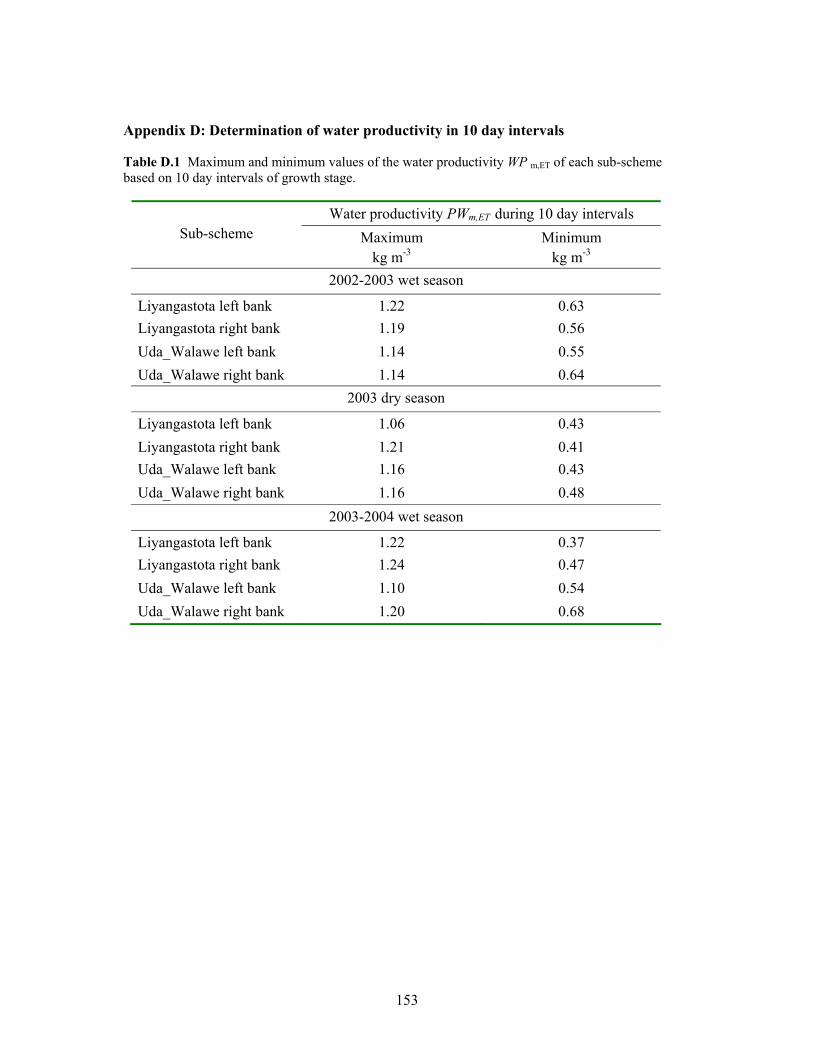
153

Appendix D: Determination of water productivity in 10 day intervals

Table D.1 Maximum and minimum values of the water productivity WP m,ET of each sub-scheme based on 10 day intervals of growth stage.

Water productivity PWm,ET during 10 day intervals Sub-scheme Maximum

kg m-3 Minimum

kg m-3 2002-2003 wet season

Liyangastota left bank 1.22 0.63 Liyangastota right bank 1.19 0.56 Uda_Walawe left bank 1.14 0.55 Uda_Walawe right bank 1.14 0.64

2003 dry season




155

Curriculum vitae

Palitha Senarath Bandara was born on 14 October 1957, in Avissawella, Sri Lanka. After secondary school, he joined the University of Peradeniya, Sri Lanka in 1977, from where he obtained the degree of B.Sc. (Engineering) civil. He joined a state-sector construction organization in the same year and in 1983 he joined the Department of Irrigation, Sri Lanka as an irrigation engineer. In 1985, he obtained his full professional qualification as a civil engineer becoming a corporate member of the Institution of Civil Engineers, UK. During the period 1997-1998, he completed the Master degree of Geoinformatics in the International Institute for Geo-Information Science and Earth Observation (ITC) in Enschede, the Netherlands. In the year 2000 he obtained the Master of Business Administration (MBA) degree from the University of Colombo, Sri Lanka.

In October 2001, he started a sandwich program for his Ph.D. studies at the University of Wageningen, the Netherlands through the sub Department of Water Resources. Presently, Palitha Bandara is working as the Deputy Director of Geoinformatics at the Department of Irrigation, Sri Lanka.

156

This research reported in this thesis was supported by the Wageningen University and Research Centre (WUR) through a ‘sandwich’ PhD fellowship. The first part of six months in Wageningen to finalize the research plan with the supervisor was financed by the ALTERRA-ILRI, Wageningen. The field work and data analysis (part 2) were carried out in Sri Lanka with the financial support and other logistics provided by the International Water Management Institute (IWMI) through their capacity building program. The final part in Wageningen to finalize the research project and the thesis was financed through the WUR sandwich program and additional funds for the extended period were provided by the ALTERRA-ILRI, Wageningen. The financial and technical support with other logistics provided by these organizations is gratefully acknowledged.

assessing irrigation performance by using remote -

Documents