assessing eolian contributions to soils in the boulder creek
TRANSCRIPT

ASSESSING EOLIAN CONTRIBUTIONS TO SOILS IN THE
BOULDER CREEK CATCHMENT, COLORADO
By
JAMES A. McCARTHY
Professor David P. Dethier, Advisor
A thesis Submitted in partial fulfillment of the requirements for the
Degree of Bachelor of Arts With Honors in Geosciences
WILLIAMS COLLEGE
Williamstown, Massachusetts
May 17, 2011
i
ABSTRACT
In high-relief environments, soil geochemistry and morphology reflect the weathering of
both parent material and materials added to weathering profiles by downslope transport and
dustfall. In the Colorado Front Range, transport is limited in alpine soils developed on stable
surfaces. In the montane zone, soils and regolith on hillslopes are mobile and mix during
downslope transport. In this study, measurement of soil texture, citrate-buffered dithionite-
extractable iron (Fed), and bulk geochemistry permitted evaluation of weathering, downslope
transport, and eolian deposition in the Critical Zone of the Boulder Creek catchment. The
accumulated mass of Fed and clay are positively correlated with deposit age in the catchment.
Stable alpine soils form from Pinedale age till and the cool, moist climate generates sufficient
acidity to develop strong horizonation. Soil morphology in the upper montane Gordon Gulch is
controlled mainly by downslope transport; soils on the north-facing slope thicken downslope and
have complex morphology. Soils on the south-facing slope are thin and overlie saprolite at a
maximum depth of 53 cm. Soils on the north-facing slope have higher clay and Fed contents than
those that face south, indicating more rapid erosion of the south-facing slope and greater
weathering on the north-facing slope. On older surfaces of low relief, soils with thick Bt horizons
develop from deeply weathered saprolite and regolith, and locally contain buried sequences and
features that suggest periglacial mass movement and slope instability in pre-Holocene time.
In soils throughout the catchment, enrichment of fine particles and low concentrations of
Fed in surface horizons suggests eolian sedimentation. Enrichment of fines is most apparent at
stable sites, but soils on lower positions on slopes are also enriched. The amount of clay and fine
silt produced in situ and the amount added from dustfall is poorly constrained, but the dustfall
rate is less than 60 g cm-2 100kyr-1. Immobile element geochemistry indicates that surface

ii
enrichment in high field strength elements (HFSE) is not uniform throughout the study area,
suggesting that the dust deposition may vary spatially and/or temporally. Ratios of the immobile
elements Ti, Zr, and Nb, suggest that surface fines are geochemically distinct from the dominant
parent materials in the catchment; however, elemental ratios may also reflect increased fines in
the surface horizons released by weathering, because Zr and Nb are preferentially enriched in
fine fractions of parent rocks in the study area. The composition of fine sediments in surface
horizons are similar to silt mantles in other basins in the Indian Peaks Wilderness Area and to
silt-sized alluvium in North Park and Middle Park to the west of the study area. Surface
enrichment of fines with low Fed and distinct immobile element ratios of low compositional
variability suggest that a substantial portion of the fine fraction of soils examined in this study
originate as dustfall, potentially derived from North Park and Middle Park.
iii
ACKNOWLEDGEMENTS
First, I would like to thank Professor David P. Dethier, who not only served as my
unbelievably helpful and ever-working thesis advisor, but also as a field guide, a mentor, a
motivator and a manager of stress. Thank you for having so much confidence in me, more than I
had in myself at times; your support made me push myself more than I would have without it,
and every new task led to deeper understanding. I would also like to thank Professor Bud Wobus
for being my second reader. He provided useful feedback and encouragement throughout the
entire process. Jay Racela, technical assistant in the Williams College Environmental Analysis
Lab, was indispensable to the completion of thesis, and is arguably the college’s best-kept secret.
Keep rocking, Jay. I would like to thank the National Science Foundation, the Boulder Creek
CZO, the Williams College Sperry Fund and the KECK Geology Consortium for providing
support necessary for the completion of this thesis. I would also like to thank all of my fellow
KECK Colorado students, especially the soils crew (Hayley, Ellie and Cianna), for assistance in
the field and for good times in the Megaron. Evan, Keith, and Caleb: thanks for keeping me sane
throughout the year. I had the pleasure of taking classes with every professor in the Geosciences
department, and I thank you all for your enthusiasm and commitment to students. All of your
classes have benefitted me in this thesis at some point, and will continue to help me in the future.
There are many friends and family who have supported me throughout my time at
Williams, far too many to mention here, but nonetheless played essential roles in getting me to
where I am. Thank you all. Lastly, I would like to thank my father, who has displayed amazing
selflessness, strength of character, and understanding through many hardships, and has always
provided me (and anyone around) with stability, advice, happiness, and love. I will forever be
impressed by you… Dad, who’s better than you?...Nobody!
iv
TABLE OF CONTENTS ABSTRACT………………………………………………………………………………………i
ACKNOWLEDGEMENTS………………………………………………………………….…iii
LIST OF FIGURES……………………………………………………………………………vii
LIST OF TABLES…………………………………………………………………………….....x
LIST OF EQUATIONS…………………………………………………………………………xi
LIST OF APPENDICES……………………………………………………………………….xii
INTRODUCTION……………………………………………………………………………….1
Background
The Critical Zone………………………………………………………………….1
Weathering processes……………………………………………………………..5
Introduction to pedology…………………………………………………………10
Soil genesis……………………………………………………………………….12
Soil physical characteristics……………………………………………………..14
Catenas…………………………………………………………………………..16
Significance of eolian additions…………………………………………………19
Identifying eolian additions
Soil texture and pedogenic iron.............................................................................23
Soil geochemistry...................................................................................................24
Study setting
Location and topography.......................................................................................26
Geologic background.............................................................................................20
Climate and vegetation..........................................................................................31

v
Paleoclimate..........................................................................................................32
Land-use history....................................................................................................34
Purpose of study................................................................................................................34
METHODS...................................................................................................................................36
Background
Field
Site selection..........................................................................................................36
Soil profile description and sampling...................................................................37
Laboratory
Sample preparation and percent moisture............................................................40
Sample partitioning...............................................................................................40
Selective dissolution analysis: dithionite-extractable iron (Fed)...........................41
Soil texture.............................................................................................................43
Soil geochemical analysis... ..................................................................................44
RESULTS.....................................................................................................................................45
Field
Green Lakes Valley................................................................................................45
Gordon Gulch........................................................................................................45
Betasso Gulch and Ward.......................................................................................48
Laboratory
Dithionite-extractable iron....................................................................................48
Soil texture.............................................................................................................49
Surface to subsurface ratios..................................................................................52

vi
Soil geochemistry................................................................................................55
DISCUSSION.............................................................................................................................62
Introduction
Weathering patterns............................................................................................62
Evidence for eolian deposition............................................................................63
Field relationships
Green Lakes valley.................................................................................................64
Gordon Gulch........................................................................................................67
Betasso Gulch, Ward, and BCW-03.......................................................................71
Establishing weathering and dustfall rates...........................................................73
Evaluating dust provenance...................................................................................77
CONCLUSIONS..........................................................................................................................81
REFERENCES CITED...............................................................................................................84
APPENDICES..............................................................................................................................87
Appendix A.........................................................................................................................89
Appendix B.......................................................................................................................109
Appendix C.......................................................................................................................121
vii
LIST OF FIGURES
Figure 1. Cross-section of the Critical Zone (Anderson et al., 2007) Figure 2. Diagram of a Critical Zone weathering profile, showing average bulk densities for different regolith components. The left side of the diagram represents a transport-limited environment, which permits development of a deep weathering profile. The right side of the diagram represents a weathering-limited environment, where mobile regolith is removed as it forms (figure by D.P. Dethier) Figure 3. The conservation of mass equation for soil [here meaning regolith] depth, h, states that the change in soil mass with time, t, is equal to the conversion of bedrock to soil because of lowering of the bedrock–soil interface less the divergence of transported soil mass. The area shown between the base of the soil at elevation, e, and the dashed line is the amount of bedrock that would be converted to soil over some specified time interval. – from Heimsath et al. (1999, p. 153)
Figure 4. The pathways and products of weathering. Adapted from McLaren and Cameron (1996) Figure 5. Relative distribution of weathered (secondary) and unweathered (primary) minerals in regolith as a function of particle size. Graphic on right portrays relative sizes of clay, silt, fine sand, and coarse sand (Schaetzl and Anderson, 2005, p. 11) Figure 6. Soil formed on late Pleistocene till in a sub-alpine environment at Silver Lake, Colorado. Soil horizon nomenclature (including both master and subhorizons) shown on the left, with red lines showing horizon boundaries. Note that the soil horizons form parallel to the geomorphic surface, which in this case dips to the left. Figure 7. Soil textural classes plotted on a ternary diagram (Schaetzl and Anderson, 2005, p. 12) Figure 8. Schematic diagram of the soil-slope units of the catena model (Birkeland, 1999).
Figure 9. Cumulative grain size frequency curves from various sources. W – local Kansas dust; Y – local Arizona dust; Z – Mongolian dust deposited in Beijing; V – Saharan dust deposited in England; X – Saharan dust collected in Barbados. With increasing distance from source, particle diameter decreases. From Pye (1987, p. 2) Figure 10. Selected mineral densities from Pye (1987, p. 44)
Figure 11. Eolian sedimentation patterns along a climatic gradient of increasing rainfall and vegetation cover. Curve A represents the dust accumulation rate and curve B represents the weathering rate of the deposited eolian material. The hyper-arid zone between W and X represents the source. “The dashed extension of curve A represents the expected accretion rate if effective dust-trapping vegetation was adjacent to the dust source.” From Pye (1987, p. 213) Figure 12. Boulder County, Colorado (http://lib.utexas.edu/maps/us_2001/colorado_ref_2001.jpg,

viii
http://www.boulder.doc.gov/gifs/boco_map.jpeg)
Figure 13. The Boulder Creek Watershed, showing locations of the three CZO study sites. (http://czo.colorado.edu/html/sites.shtml) Figure 14. Topographic map of the Betasso catchment, Colorado. (http://czo.colorado.edu/html/bt.shtml)
Figure 15. Topographic map of Gordon Gulch, Colorado.(http://czo.colorado.edu/html/gg.shtml) Figure 16. Topographic map of Green Lakes Valley, Colorado.
Figure 17. Temperature, precipitation, and vegetation patterns in the Front Range. From Birkeland et al. (2003, modified from Veblen and Lorenz (1991)).
Figure 18. Lower limits of Pleistocene glaciation (~22 ka – 18 ka) in the Colorado Front Range, indicated by glacial deposits (dotted pattern). The gray pattern shows the modern surface of low relief. Approximate locations of Green Lakes Valley (GL), Gordon Gulch (GG), and Betasso Gulch (BG) shown in red. Modified from Birkeland (2003).
Figure 19. The Boulder Creek catchment, showing in green the locations of soil pits that we dug, described and sampled for this study.
Figure 20. Soil pit description and sampling at the Ward road-cut site. Pictured from left to right are Cianna Wyshnytzky (Amherst College), Ellie Maley (Smith College), and Hayley Corson-Rikert (Wesleyan University).
Figure 21. Using the atomic absorption spectrometer (AAS) to analyze dithionite-extractable iron (Fed) in the Williams College Environmental Analysis Laboratory. Photograph by Jay Racela.
Figure 22. Three soil profiles from the Boulder Creek CZO. SLQ-01 is a soil from the Green Lakes basin formed in Pinedale glacial till (~15 ka), reaching a depth of approximately 110 cm in the field of view. SFT-1B is a 68 cm-thick soil from the south-facing slope of lower Gordon Gulch (saprolite boundary at 38 cm). NFT-01 is a 188 cm-thick soil from the north-facing slope of Gordon Gulch.
Figure 23. A typical middle Gordon Gulch soil, MGG-02, with a deeply weathered saprolite (Cr) and thin Cox. The profile shown here is 115 cm deep. Note the preservation of the rock structure in the saprolite, indicated by the more and less-altered zones dipping parallel to the foliation (bounded by black dashed lines).
ix
Figure 24. Fed accumulation rate, determined by using total profile accumulated Fed content of four soils of known age. The soil from Betasso Gulch (red bullet) formed from deep, weathered colluvium and a substantial and uncertain portion of the Fe2O3 content is inherited. For this reason, the profile was not used to fit the curve. See Appendix A for complete profile descriptions
Figure 25. Total profile clay content plotted as a function of total profile Fed content of sampled soil profiles.
Figure 26. Total profile accumulated clay content plotted as a function of total profile accumulated Fed content of sampled soil profiles.
Figure 27. Diagram of NFT-03, displaying concentrations of Fed and fine particles (<11 µm) down profile. The A and Bw horizons are enriched in fine particles.
Figure 28. Clay and Fed concentrations at BCW_SLQ-01. Individual soil horizons are labeled.
Figure 29. Concentration of fine particles (<11 µm) and Fed at GL1-01. Individual soil horizons are labeled.
Figure 30. Concentrations of Zr, Y (x 10), Ce, and Ti at BCW_SLQ-01. Soil horizons are labeled.
Figure 31. Total profile accumulated Fed content and total profile clay content along the two Gordon Gulch catenas. The north-facing slope is in black and the south-facing slope in red. The filled markers and solid lines represent Fed content, and the hollow markers and dashed lines represent clay content.
Figure 32. Concentration of fine particles (<11 µm) and Fed at NFT-01. Individual soil horizons are labeled.
Figure 33. Concentration of clay and Fed at WRC-01. Individual soil horizons are labeled. Note the strong correlation between clay and Fed.
Figure 34. Concentration of fine particles (<11 µm) and Fed at BCW-03.
Figure 35. Total profile clay and Fed accumulation rate, determined using soils of known age. Soil profiles are labeled.
Figure 36. Ratios of Ti/Zr plotted against Ti/Nb from Muhs and Benedict (2006). Compositional fields of gneissic and granitic units of the Indian Peaks and Boulder Creek areas are shown. Hollow markers are the silt fraction of surface horizons collected by Muhs and Benedict (2006) in the Indian Peaks wilderness area, Colorado Front Range. Solid black markers are the fine fraction (<150 µm or <63 µm) of surface horizons from this study. The red and green markers represent the average composition (n=10 for each) of the fine fractions of Boulder Creek Granodiorite (BCG) and Silver Plume Granite (SPG), respectively. BCG and SPG samples were collected in the Boulder Creek catchment and analyzed by D.P. Dethier.

x
LIST OF TABLES Table 1. Chemical composition and color of pedogenic iron compounds. Colors are described according to the Munsell soil color scheme, described below. Adapted from Birkeland (1999). Table 2. Soil master horizon nomenclature (Birkeland, 1999, p. 5; Jenny, 1980, p.6) Table 3. Subhorizon nomenclature from Birkeland (1999, p. 5-6) Table 4. Particle size classes (Birkeland, 1999) Table 5. Mean silt, clay, <11µm and Fed values, in percent, of both surface and subsurface horizons at all sites, stable sites, and the Gordon Gulch catenas (GG). At each site, a thickness-weighted mean was calculated for the subsurface, and these means were then averaged. The north-facing and south-facing catenas are shown separately as “NFT” and “SFT”. Table 6. Mean A-horizon to C-horizon ratios of percent silt, clay, <11µm fraction, and Fed at all site, stable sites, and Gordon Gulch (GG). The north-facing catena (NFT) and south-facing catena (SFT) are shown separately as well. 1 sigma (STDEV) is also shown. Table 7. A-horizon:C-horizon ratios of the major oxides. Table 8. A-horizon:C-horizon ratios of high field strength elements (HFSE). Table 9. A-horizon:C-horizon ratios of light rare earth elements (LREE). Table 10. A-horizon:C-horizon ratios of heavy rare earth elements (HREE). Table 11. Fine-fraction to coarse-fraction ratios of the major oxides. Mean values of all sites, surface horizons, and subsurface horizons are provided. “Subsurface” here denotes parent material (C) horizons. Table 12. Fine-fraction to coarse-fraction ratios of HFSE. Mean values of all sites, surface horizons, and subsurface horizons are provided. Table 13. Fine-fraction to coarse-fraction ratios of LREE. Mean values of all sites, surface horizons, and subsurface horizons are provided. Table 14. Fine-fraction to coarse-fraction ratios of HREE. Mean values of all sites, surface horizons, and subsurface horizons are provided. Table 15. Select data from SLQ-01 that was employed to determine the amount of Fed produced in situ and translocated from above.
xi
LIST OF EQUATIONS Equation 1. Regolith production function (Heimsath et al., 1999) Equation 2. Silicate hydrolysis (Birkeland, 1999, p. 60) Equation 3. Soil formation function (Jenny, 1941) Equation 4. Soil moisture formula

xii
LIST OF APPENDICES
Appendix A. Annotated photographs of soil profiles sampled for this study, with profile descriptions and basic chemical data. Appendix B. Complete table of soil analysis data Appendix C. Complete table of bulk geochemical analysis certificated by Acme Analytical Laboratories, Ltd.

1
INTRODUCTION
Background The Critical Zone
The Critical Zone (Anderson et al., 2007) is the upper part of the earth’s crust where the
biosphere, atmosphere, hydrosphere, and rock materials interact. Extending from the base of
groundwater to the top of the vegetation canopy, the complex processes occurring in the Critical
Zone (Fig. 1) release raw materials from minerals and create substrates for terrestrial life,
supporting microbial, plant, and faunal activity. Solar radiation and tectonism provide energy for
the system and drive the physical and chemical processes that lead to the interaction of these
various spheres (Anderson et al., 2008).
Figure 1. Cross-section of the Critical Zone (Anderson et al., 2007)

2
The Critical Zone can be thought of as a bottom-up feed-through reactor, where physical
and chemical weathering processes act on fresh rock material being supplied by uplift and
erosion (Anderson et al., 2007). Simultaneously, physical erosion and chemical denudation
processes transport mass out of the system. Rates of weathering and denudation together
determine the thickness of the Critical Zone (Anderson et al., 2007).
In transport-limited systems, weathering rates exceed denudation and deep weathering
profiles may develop (Anderson et al., 2007). Bedrock will first be oxidized along fractures with
exposure to atmospheric O2 and gases dissolved in percolating rainwater. Over time, continued
weathering produces an overlying zone of oxidized bedrock that may be meters thick, and has a
density slightly less than fresh bedrock. Additional weathering gradually breaks down rock
structure, leading to the formation of saprolite and then regolith. Saprolite is isovolumetrically
weathered bedrock that retains the original rock fabric and has sufficient strength that it cannot
be transported by mass movement. The structure of the rock, however, has been greatly
weakened by weathering processes (primarily alteration of ferromagnesian minerals, feldspars
and micas), and the saprolite has a very low cohesive strength. Mobile regolith gradually forms
from saprolite or oxidized bedrock and is defined as loose unconsolidated rock materials that can
be transported (Anderson et al., 2007; Schaetzl and Anderson, 2005). Soil is the highly
weathered, top-most layer of the regolith, but is distinct because of its unique layered habit.
These layers, termed horizons, are the result of more intense weathering conditions at the
surface, and represent downward transport of chemical weathering products and organic
additions from the biosphere (Anderson and Anderson, 2010). The development and sequence
of soil horizons is broadly parallel in different environments.

3
Figure 2. Diagram of a Critical Zone weathering profile developed in granitic bedrock, showing average bulk densities for different layers. The left side of the diagram represents a transport-limited environment, which permits development of a deep weathering profile. The right side of the diagram represents a weathering-limited environment, where mobile regolith is removed as it forms from oxidized bedrock or saprolite (figure by D.P. Dethier).
In weathering profiles developed from bedrock (Fig. 2), the bottom-up sequence of
bedrock, oxidized bedrock, saprolite, regolith, and soil records the downward advancement of
the weathering front and stirring and fracturing processes over time. The base of oxidized
bedrock denotes the weathering front, and the overlying materials are increasingly more
weathered near the surface. In weathering-limited systems, denudation rates exceed weathering
rates and physical erosion rates are limited by the rate of regolith production (Anderson et al.,
2007). As mobile regolith forms, it is subject to transport processes, incorporating more material
as it moves down-slope. The balance of transport-limited and weathering-limited environments is
largely determined by topographic and climatic factors.

4
The Critical Zone is at steady state when “rock materials are removed at the same rate
that they are replenished (Brantley, 2008, p. 1454).” That is, steady state is achieved when the
regolith transport rate equals regolith production rate. The distribution of steady-state conditions
in landscapes is not well understood. Landscapes are dynamic; the tectonic and climatic
processes that lead to their formation are not constant through time, and perturbations caused by
changing conditions create non-steady state conditions in an environment or on local hillslopes.
The presence of weathering-limited and transport-limited environments suggests that steady state
conditions are rarely achieved on an entire landscape scale, especially in high-relief
environments (Jungers et al., 2009). In hilly landscapes, regolith may be non-uniform: “bedrock
often crops out in locally steep areas, soils are typically thin to absent on narrow ridge crests, and
soil tends to accumulate to considerable depths in valleys (Heimsath et al., 1999, p.
152).”Assuming conservation of mass within a regolith column, Heimsath et al. (1999) defined
the steady-state balance between regolith transport and production with the following equation:
Figure 3/ Equation 1. The conservation of mass equation for soil [here meaning regolith] depth, h, states that the change in soil [depth] with time, t, is equal to the conversion of bedrock to soil because of lowering of the bedrock–soil interface [minus] the divergence of transported soil, [modified by the density change]. The area shown between the base of the soil at elevation, e, and the dashed line is the amount of bedrock that would be converted to soil over some specified time interval. – from Heimsath et al. (1999, p. 153)
5
where e is the elevation of the bedrock-regolith interface, t is time, h is the regolith thickness, ρs
is the soil (regolith) density, ρr is the rock bulk density, and qs is sediment flux. Sediment flux
here is assumed to be carried out by diffusive transport processes (e.g. biogenic transport and
creep), and rates are determined by a diffusion coefficient K and proportional to slope curvature
(Heimsath et al., 1997). It is important to note here, that Heimsath et al. (1997, p. 358) define
soil to be “distinct colluvial material, lacking relict rock structure and derived from underlying
bedrock.” Therefore, soil as Heimsath et al. define it refers to the entire regolith column, and not
simply the topmost layered portion of the regolith. In this study, only the topmost, layered
portion of the regolith is defined as soil.
The above regolith production function has been used widely, often assuming steady state
conditions so that regolith thickness, h, is constant through time and the regolith-production
function is equal to the erosion rate. That steady-state occurs locally is an important distinction,
as soil thickness may vary widely within a catchment. A distinction here might be made, then,
that while steady-state may occur locally, the greater catchment area is often in disequilibrium.
Field observations, coupled with cosmogenic isotope studies (e.g. using 10Be as a geomorphic
tracer), have comprised studies of regolith depth with changing geomorphic conditions; the
relationship of regolith depth to hillslope curvature suggests that regolith production rate is
inversely proportional to the depth of regolith (Heimsath et al., 1999).
Weathering processes
Weathering processes disaggregate and chemically decompose rock material from the top
down, turning fresh bedrock to “more stable forms under the variable conditions of moisture,
temperature, and biological activity that prevail at the surface (Birkeland, 1999, p. 53).” The rate
of chemical weathering depends on mineral species, the delivery of reactants (usually as aqueous

6
species in percolating rain water) to unweathered mineral surfaces, and the removal of
byproducts from the system. Thus, mineral dissolution rates are determined by reaction kinetics
and transport (Anderson et al., 2007). Reaction kinetics are dependent on the concentration of
reactants in soil water, the temperature, and bedrock mineralogy, as some minerals dissolve more
readily than others. Transport of aqueous species is affected by the amount and rate at which
water is transmitted through the Critical Zone; this factor, termed hydraulic conductivity, is
largely dependent on the size and distribution of flow pathways in the regolith and underlying
bedrock (McLaren and Cameron, 1996). Physical weathering serves to increase chemical
weathering, as it increases the reactive surface area of the rock materials, and creates more
pathways for water.
Figure 4. The pathways and products of weathering. Adapted from McLaren and Cameron (1996).
The products of chemical weathering (Fig. 4) are secondary phyllosilicate minerals
(clays), iron and aluminum oxides and oxyhydroxides, and aqueous cations such as Ca2+, Na+,

7
and Si4+ (Birkeland, 1999). Congruent dissolution results in the complete dissolution of the
primary mineral into aqueous species, but is restricted to a limited number of minerals, as most
minerals are not completely soluble at surface temperatures and pressures. Incongruent
dissolution, in which primary minerals weather to new, solid compounds, is a dominant
weathering process in regolith formation. The most important incongruent dissolution reaction is
silicate hydrolysis, which follows the general formula (Birkeland, 1999, p. 60):
Aluminosilicate mineral + H2O + H2CO3(aq) → clay mineral + cations(aq) + OH- (aq) +
HCO3-(aq) + H4SiO4(aq) (eq. 2)
The soluble products can be leached out of the system, resulting in a loss of mass (Schaetzl and
Anderson, 2005). Alternatively, soluble cations (especially K+ and Mg2+) may be taken up by
vegetation, incorporated in clay minerals, or may be adsorbed onto organic colloids (Birkeland,
1999). Iron and aluminum are relatively immobile (insoluble) in soils of average pH range (~5-
9), so where iron and aluminum are released by weathering, they may be oxidized and or
hydrated to produce secondary oxide or hydroxide compounds (Birkeland, 1999).
Table 1. Chemical composition and color of pedogenic iron compounds. Colors are described according to the Munsell soil color scheme, described below. Adapted from Birkeland (1999).
Mineral Formula Munsell Color
Goethite α-FeOOH 7.5YR – 2.5Y
Lepidocrocite γ-FeOOH 5YR – 7.5YR, value ≥ 6
Hematite α-Fe2O3 7.5R – 5YR
Maghemite γ-Fe2O3 2.5YR – 5YR
Ferrihydrite Fe5HO8•4H2O or Fe5(O4H3)3 5YR – 7.5YR, value ≥ 6

8
The concentrations of various pedogenic iron compounds (Table 1) at a given location
indicate the degree of weathering that has taken place in the Critical Zone. Iron oxides in
appreciable concentrations will make the soil and regolith noticeably red in color; thus,
secondary iron oxides are particularly useful to pedologists, because they permit interpretation of
weathering regimes in the field. Because weathering is a time-dependent process, pedogenic iron
concentrations also permit relative dating of soil profiles within an environment. At stable sites,
chronosequence studies have shown that the amount of pedogenic iron oxide and clay increase as
soils become older (McFadden and Hendricks, 1985). Goethite and hematite are the most
common iron products in well drained, oxidizing conditions (Birkeland, 1999). Soils in oxidizing
environments are increasingly redder with age because of (1) continued accumulation of iron
oxides through weathering and (2) conversion of other iron-oxide species (such as ferrihydrite)
to hematite, which has the strongest red coloring (McFadden and Hendricks, 1985).
Lepidocrocite forms in anaerobic environments, where iron is mainly in its reduced form, Fe2+
(Birkeland, 1999). The rate of iron accumulation is initially rapid as ferromagnesian minerals are
readily weathered in the soil environment. Weathering rates decrease over time as the more
easily weathered iron-bearing minerals are depleted relative to resistant mineral species.
Furthermore, clays, organic matter, and iron and aluminum oxides coat fresh mineral surfaces as
weathering increases, effectively reducing mineral dissolution rates (McFadden and Hendricks,
1985).
The crystalline products of weathering (Fig. 5) are of sufficiently smaller size than
primary minerals and as a result are more easily transported. This leads to the development of
soil horizons, which is discussed below.

9
Figure 5. Relative distribution of weathered (secondary) and unweathered (primary) minerals in regolith as a function of particle size. Graphic on right portrays relative sizes of clay, silt, fine sand, and coarse sand (Schaetzl and Anderson, 2005, p. 11).
The nature of the Critical Zone is such that optimal weathering conditions rarely occur
(Anderson et al., 2007). Hydraulic conductivity is the highest at the surface, but much of the
surficial regolith is previously weathered, resulting in a lack of weatherable minerals. At the base
of the Critical Zone there is a greater supply of weatherable material, but fluid flow pathways are
not as extensive and fluids are not as reactive as at the surface (Anderson et al., 2007). Enhanced
weathering capacity at the surface is in large part due to increased interactions with the biosphere
and atmosphere, as biologic agents in high concentrations promote weathering and reactive
atmospheric gases are dissolved in rain water (Anderson and Anderson, 2010). Biologic
disturbance of rock materials (bioturbation), and physical weathering processes such as freeze-
thaw are greatest near the surface, and enhance weathering (Heimsath et al., 1999). As these
processes are limited with increasing depth the efficiency of transport decreases with increasing
depth as well. Perhaps as a result, the rate of regolith production apparently varies inversely with
the thickness of overlying material (Heimsath et al., 1999).
Introduction to pedology

10
Soils, as I use them here, are defined primarily by their layered morphology. Birkeland
(1999, p.2) used the following definition: “a soil is a natural body consisting of layers (horizons)
of mineral and/or organic constituents of variable thicknesses, which differ from the parent
materials in their morphological, physical, chemical, and mineralogical properties and their
biological characteristics.” This definition notes that the layering of soils is a basic property and
signals that many different processes act on the parent material and lead to the formation of the
soil landscape. Furthermore, Birkeland’s definition suggests that soil has distinct physical and
chemical properties that allow it to be distinguished from the underlying parent material.
Soil horizons typically develop parallel to the geomorphic surface, as soil forming
processes extend downward into the parent material (Birkeland, 1999). The development of soil
horizons in differing landscapes follows parallel paths, and basic horizon nomenclature (Table 2)
is similar in various classification systems.
Table 2 Soil master horizon nomenclature (adapted from Birkeland, 1999, p. 5; (Jenny, 1980, p.6))
Name Horizon Description O Surface accumulation of organic material. Dark in color due to organics A Accumulation of humic material, but dominantly mineral material. At surface or
below O-horizon E Subsurface horizon. Zone of eluviation. Leached of organics, clays, Al + Fe
sesquioxides B Zone of illuviation. Little evidence of original rock structure. Accumulation of clays,
organics, Al + Fe sesquioxides, carbonates (minor), and/or gypsum. Underlies A or E C Simulates the original rock or parent material from which and in which A and B
evolved R Bedrock underlying the soil
One or several of the master horizons may be absent from a soil, reflecting variation in soil
forming factors. Several other master horizons are not mentioned here as their formation
represents extreme environmental conditions not seen in the study area. Soil is a continuum, both
vertically and laterally, and thus sharp boundaries (between both horizons and soil pedons) are

11
difficult to define (Birkeland, 1999). Specific horizon-defining criteria have been developed to
remove ambiguity, but many require laboratory analysis; the criteria are somewhat arbitrarily
defined and do not hold particular importance here. Even with specific criteria, boundaries
between horizons are quite diffuse at many sites and a depth range may demonstrate traits of
multiple master horizons. In this case, pedologists use two master horizon labels to define the
horizon and exemplify its transitional nature (e.g. AB, BC).
Subhorizon distinctions (Table 3) allow description of the master horizons with greater
specificity.:
Table 3. Subhorizon nomenclature from Birkeland (1999, p. 5-6)
Name Subhorizon Description b Buried soil horizon with major features formed prior to burial h Illuvial accumulation of organic matter. Most commonly used with B horizons, but
sometimes Ah horizons are described j Denotes incipient development for that particular master horizon; its properties are not
fully expressed (e.g. Ej) t Modifies B horizons. Indicates translocation or in-situ formation of alumino-silicate
clays into B-horizon. Bt will have measurably more clay than overlying horizon. w Modifies B horizons. Bw suggests development of stronger oxidation colors and soil
structure relative to C horizon, but has little evidence of illuvial accumulation ox Modifies unconsolidated C horizons. Cox horizon is oxidized, but does not meet
criteria for Bw horizon r Modifies consolidated C horizons. Cr is used to describe in situ weathered bedrock,
demonstrated by preservation of original rock features (i.e. saprolite). For many soils, multiple subhorizon descriptors can be used to most effectively describe a
horizon. For instance, a Crt horizon describes a saprolite that has accumulated clay into the
weathered saprolite structure, due to in situ weathering or translocation. Numbers may be used to
designate distinct horizons that have similar designations (e.g. Bw1, Bw2). Buried horizons are
recognized by having primary pedogenic features, but are covered by younger sediments that are
not of the same weathering sequence (Schaetzl and Anderson, 2005). For example, an easily
identified buried soil horizon is an Ab horizon that underlies an A horizon and Bw horizon of
12
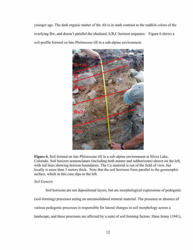
younger age. The dark organic matter of the Ab is in stark contrast to the reddish colors of the
overlying Bw, and doesn’t parallel the idealized A,B,C horizon sequence. Figure 6 shows a
soil-profile formed on late-Pleistocene till in a sub-alpine environment.
Figure 6. Soil formed on late Pleistocene till in a sub-alpine environment at Silver Lake, Colorado. Soil horizon nomenclature (including both master and subhorizons) shown on the left, with red lines showing horizon boundaries. The Cu material is out of the field of view, but locally is more than 3 meters thick. Note that the soil horizons form parallel to the geomorphic surface, which in this case dips to the left.
Soil Genesis
Soil horizons are not depositional layers, but are morphological expressions of pedogenic
(soil-forming) processes acting on unconsolidated mineral material. The presence or absence of
various pedogenic processes is responsible for lateral changes in soil morphology across a
landscape, and these processes are affected by a suite of soil forming factors. Hans Jenny (1941),

13
one of the most influential 20th century pedologists, looked at soils as a system, and reduced the
number of important soil forming factors to a simple relationship, claiming:
Soil Formation = f(cl,o,r,p,t) (Eq. 3)
where cl is climate,
o is organisms,
r is relief,
p is parent material,
and t is time.
Climate accounts for a region’s temperature and moisture regime. Organisms and relief refer to
the influence of biological organisms (e.g. soil microbes and plants) and topography (e.g. slope
aspect), respectively, on soil formation. The effect of parent material on soil formation is
potentially more intuitive than the other variables, as changes in rock mineralogy and weathering
patterns can clearly affect the physical and chemical properties of the soil which forms from it.
Time is an important soil forming factor because the processes that produce different soil
horizons require sufficient time to be carried out. Jenny’s soil forming factors suggest that soils
are defined by the interaction between rock materials, and the biosphere, hydrosphere, and
atmosphere. Jenny (1941, p.15), however, argued further, “for a given combination of cl, o, r, p,
and t, the state of the soil system is fixed; only one type of soil exists under these conditions.” If
this assertion is correct, soils can be used as an instructional index, and can be applied to
geomorphology, (paleo)ecology, and (paleo)climatology. With an understanding of a particular
soil forming environment, a soil provides a wealth of knowledge to the geomorphologist.
Jenny’s soil formation function assumes equilibrium conditions on a stable substrate. In this
model, parent material must be defined broadly as the mineral material that the weathering front

14
first advances into and pedogenic (soil-forming) processes then act on. The range of soil parent
materials makes it so that the differentiation between the weathering front and the base of the soil
profile may not be clear. Parent materials can be consolidated or unconsolidated; in some cases,
parent material may be sufficiently uniform (e.g. till or loess) that the weathering front is parallel
with the base of the soil profile. In bedrock (e.g. Boulder Creek Granodiorite), saprolite may
show evidence of some pedogenic horizonation (e.g. clay accumulation), but its intact rock
structure denotes a C-horizon distinction. In some cases, parent material may be previously
weathered before deposition (e.g. colluvium). To understand the pedogenesis of a soil, therefore,
one must be able to distinguish it from its parent, and that requires characterizing the parent
material (Birkeland, 1999).
Soil physical characteristics
Physical characteristics of the soil that are capable of being observed in the field indicate
the degree of pedogenesis that has taken place in a soil. Two of the most telling characteristics
are soil texture and color. Soil texture describes the particle-size distribution of the fine earth
fraction (<2 mm) of a soil. Particles are divided into three size categories: sand, silt, and clay
(Table 3). In this case, “clay” refers only to the size of the particle and is distinguished from clay
minerals, the products of silicate hydrolysis (Birkeland, 1999; Schaetzl and Anderson, 2005).
Relative proportions by mass of sand, silt, and clay define specific soil textural classes (Fig. 7).
Table 3. Particle size classes (Birkeland, 1999).
Sand 2.0mm – 0.05mm Silt 0.05mm - .002mm Clay < 0.002mm (< 2µm)

15
Figure 7. Soil textural classes plotted on a ternary diagram (Schaetzl and Anderson, 2005, p. 12)
Soil texture is an important characteristic for many reasons. Generally, water infiltration
and transport is faster in coarse-textured soils than fine-textured soils (Schaetzl and Anderson,
2005). Infiltration rate is partly related to surface area per unit volume, which increases
exponentially in finer-textured soils. High surface areas in fine-textured soils makes them the
most reactive, and they weather more quickly than coarse-textured soils as a result (Birkeland,
1999; Schaetzl and Anderson, 2005). Within a soil-profile, more clayey textures in B-horizons
are indicators of the genesis and translocation of clay minerals in a soil, and therefore texture can
be used in estimating the age of a soil (Birkeland, 1999).
Color is arguably the most important soil physical characteristic in making field
determinations, because color is the most obvious indicator of the presence or absence of
pedogenic processes in a soil environment (Birkeland, 1999). Soil color description has been
standardized, and is done using the hue, value, and chroma values of the Munsell color system
(e.g. “10YR 3/4”) (Schaetzl and Anderson, 2005). A-horizons are typically dark (low value and

16
chroma) because of the presence of organic matter. E-horizons are indicative of a leaching
environment and the grey color is due to the removal of iron and absence of weathering products
(Schaetzl and Anderson, 2005). B-horizons are defined by their evidence of illuviation of
weathering products. The brown to red colors typical of B-horizons are evidence of various
pedogenic iron compounds discussed above (Table 1) and sometimes transported organic matter.
Intensity of soil colors, however, is not a complete indicator of the amount of color-
forming materials present in a horizon as soil texture affects the expression of color (Birkeland,
1999). That is, coarser-grained soils have less surface area than finer-grained soils, and require
less total weathering products to coat grain surfaces and express strong colors. As the mass of
weathering products can be correlated with the age of a soil, a coarser-textured soil will take less
time to develop strong horizonation than a finer-textured soil (Schaetzl and Anderson, 2005).
Similarly, thicker horizons will take longer to express strong coloring than thinner horizons
(assuming all other conditions are constant).
Catenas
Jenny’s soil formation model does not accurately represent soils on hillslope, as slopes
represent unstable landscapes. The bottom-up reactor model for regolith and soil formation
assumes that the parent materials in the system derive only from the weathering of underlying
bedrock or sediment. However, soil profiles on slopes are distinctly related to the soils above and
below because of the influence of slope-controlled transport mechanisms. The term catena
describes a sequence of soils on a slope, emphasizing that their variation is due to changes in
both slope gradient and position. Terminology and descriptions below are adopted from
Birkeland (1999).

17
Catenas may be open or closed systems: in an open system sediments are transported off
the slope; in closed systems a depression at the base of the slope prevents transport of sediment
and deep colluvium develops. In either system, a simple five unit soil-slope relationship helps
describe much of the variability in the system (Fig. 8).
Figure 8. Schematic diagram of the soil-slope units of the catena model. Mobile regolith here may include soils and buried soils. Adapted from Birkeland (1999).
Regolith and soil thicknesses are thinnest at the shoulder and backslope, and gradually
thicken, reaching a maximum at the toeslope. There is also a chemical gradient along slopes.
This gradient is driven partly by the physical transport of the mobile regolith, but also due to
hydrologic factors; clay minerals and dissolved cations in a soil column may be transported
down slope by throughflow water, accumulating at the base of the slope. The surface and
shoulder, then, comprise an eluvial zone and the footslope and toeslope comprise an illuvial
zone. The backslope represents a transluvial zone, indicating that the regolith has not reached a
stable depositional surface. In the field, thicker and more clay-rich B-horizons may be observed
at the concave slope positions due to these transport mechanisms. Climatic conditions determine
both the mobility of soil materials and chemical constituents, and thus the effects of throughflow

18
on pedogenesis vary spatially. Stronger horizonation may occur at the base of slopes in the
illuvial zone not only due to the influx of weatherable materials, but also due to increased soil-
moisture status via throughflow water.
Whether thicker B-horizons at concave slope positions are the result of higher degrees of
pedogenesis is debated, because downslope transport of the mobile layer may be episodic,
mediated by climate; and regolith that eventually arrives at the footslope/toeslope may have been
previously weathered before deposition. Models of sediment flux generally assume that hillslope
processes are constant through time, but episodic transport suggests more stochastic conditions
in real environments (Anderson and Anderson, 2010). Episodic transport may result in the burial
of soils at the base of the slope, and current soils in these positions may be forming from
colluvial parent materials rather than from bedrock. Thus, morphological differences along the
slope gradient may not represent changes in the strength of pedogenesis but actually a change in
parent material.
Regolith transport on hillslopes is the result of many processes, which operate in broadly
parallel ways: a mechanism disturbs the soil or regolith and “randomly” oriented movement of
the particles occur. Particles travel longer paths downhill than uphill due to the influence of
gravity, and thus net downslope transport occurs (Anderson and Anderson, 2010). Disruption of
the regolith can be at the surface or at depth, and the scale of these processes varies widely.
Physical disruption processes include rainsplash, frost heave and gelifluction. Biologic disruption
of the regolith (bioturbation) includes animal burrowing, tree throw, ant hill creation and
displacement of soil by root growth.
Significance of eolian additions

19
Particle transport by wind has broad environmental significance. Wind erosion can
decimate agricultural soils and dust may create environmental health concerns. In depositional
settings, dust can enrich soils and improve agricultural efficiency. In natural settings, dust
additions have broad effects on soil pedogenesis. The influence of dust in soil formation,
however, is conceptually overlooked by Jenny’s soil formation function and the Critical Zone
reactor model. In the bottom-up reactor model, the least weathered mineral material is at the
base of the weathering front and the regolith/soil columns forms out of the underlying parent
material. Dust additions, however, provide mineral material to the surface of the Critical Zone
reactor.
The effects of eolian additions on soils are varied due to eolian sedimentation patterns.
Closer to the sediment source, eolian deposits are thicker and coarser-grained; with increased
downwind distance, eolian deposits become thinner and more fine-grained (Birkeland, 1999). In
other words, eolian sediments exhibit downwind sorting. Prevailing wind directions and
velocities and grain-size determine the distribution of eolian sediments in a particular
environment. Globally, most eolian sediments are composed of particles less than 0.1 mm (100
µm) (Pye, 1987).

20
Figure 9. Cumulative grain size frequency curves from various sources. W – local Kansas dust; Y – local Arizona dust; Z – Mongolian dust deposited in Beijing; V – Saharan dust deposited in England; X – Saharan dust collected in Barbados. With increasing distance from source, dust particle diameter decreases. From Pye (1987, p. 2)
Silt and clay sized materials are more easily entrained than sands due to smaller mass, and thus
have a wider distribution from a central source. Indeed, clay-rich dust is capable of traveling
thousands of kilometers; geochemical analysis has shown that dust from the Sahara and Sahel
regions of Africa enriches soils on western Atlantic islands (Muhs et al., 2007a). Deposition of
entrained particles is partly determined by mass; however, the particle density is also significant.
That is, denser particles will be deposited closer to the source than less dense particles of the
same size. Particle density is a function of particle mineralogy (Fig. 10); therefore, downwind
sorting of eolian particles is also likely to result in mineral and thus chemical fractionation.

21
Figure 10. Selected mineral densities from Pye (1987, p. 44)
Ferromagnesian minerals, especially magnetite and ilmenite, have high densities and may be
deposited nearer to the source than felsic minerals. Eolian sorting, therefore, may lead to
enrichment of certain environments in iron-bearing minerals, which potentially affects soil
morphology. If eolian sorting and deposition results in chemical differentiation in an
environment of varied parent materials, homogenization of near-surface sediment may occur
(Reynolds et al., 2006b).
The enrichment of eolian silt and clay affects the “mineralogy, chemistry, nutrient status,
and moisture-holding capacity of soils (Muhs and Benedict, 2006, p. 120),” and thus “may
control the rate and direction of pedogenesis (Mason and Jacobs, 1998, p. 1135).” For this
reason, characterizing the rate of eolian inputs is important for soil study. The transport,
deposition, and subsequent weathering of eolian materials are determined by climate (Fig. 11).
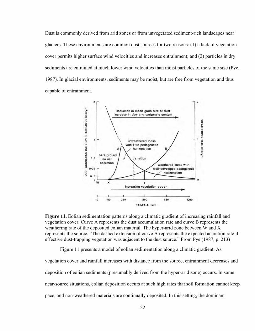
22
Dust is commonly derived from arid zones or from unvegetated sediment-rich landscapes near
glaciers. These environments are common dust sources for two reasons: (1) a lack of vegetation
cover permits higher surface wind velocities and increases entrainment; and (2) particles in dry
sediments are entrained at much lower wind velocities than moist particles of the same size (Pye,
1987). In glacial environments, sediments may be moist, but are free from vegetation and thus
capable of entrainment.
Figure 11. Eolian sedimentation patterns along a climatic gradient of increasing rainfall and vegetation cover. Curve A represents the dust accumulation rate and curve B represents the weathering rate of the deposited eolian material. The hyper-arid zone between W and X represents the source. “The dashed extension of curve A represents the expected accretion rate if effective dust-trapping vegetation was adjacent to the dust source.” From Pye (1987, p. 213)
Figure 11 presents a model of eolian sedimentation along a climatic gradient. As
vegetation cover and rainfall increases with distance from the source, entrainment decreases and
deposition of eolian sediments (presumably derived from the hyper-arid zone) occurs. In some
near-source situations, eolian deposition occurs at such high rates that soil formation cannot keep
pace, and non-weathered materials are continually deposited. In this setting, the dominant

23
physical features of the substrate are primarily sedimentologic and not pedogenic (Birkeland,
1999). At a distance, fine sediments are deposited at lower rates, and soil formation parallels or
exceeds deposition. It is this depositional scheme that leads to the development of cumulative
soils, suggesting modification of the typical Critical Zone model. The original parent material of
the soil may itself be eolian, indicating times of greater accumulation rate in the past that
overwhelmed soil formation (Birkeland, 1999); with increased distance from the dust source,
however, accumulation rates are small enough so that the original parent material (e.g. crystalline
bedrock) primarily influences pedogenesis (Muhs et al., 2008). Dust inputs are rapidly weathered
at the surface, and potentially offset losses from the weathering of the original parent material
(Mason and Jacobs, 1998). The mineralogy and grain size of the dust determine the effect on
pedogenesis. For example, inputs of fine clays can lead to the development of Bt horizons on
previously formed sand dunes; without this influx of clay minerals, development of Bt horizons
on resistant quartz sands would not occur (Yaalon and Ganor, 1973). Modification of the soil
profile can be so slight that eolian additions are barely detectable in the field. Yaalon and Ganor
(1973) termed this “eolian contamination” to exemplify that the eolian effects on pedogenesis are
secondary.
Identifying eolian additions
The effects of dustfall on soil pedogenesis are varied due to differing climate, dust
mineralogy and accumulation rate. For this reason, soil morphology alone often is insufficient to
indicate eolian deposition in an area. This is especially true in environments where dustfall rates
are sufficiently low that soil formation exceeds deposition. In these situations, textural and
geochemical data may indicate eolian additions to soils.
Soil texture and pedogenic iron

24
Dustfall may be indicated by the relationship between soil texture and pedogenic iron
concentrations in soil. As previously mentioned, pedogenic iron compounds and clays are
weathering products, and typically increase in concentration with soil age and/or stronger
weathering regime (McFadden and Hendricks, 1985). In stable soils, pedogenic iron compounds
and clays are expected to be positively correlated throughout the profile. Furthermore, pedogenic
iron and clay concentrations are expected to be highest in the B-horizons, and depleted in A-
horizons (and further depleted in E-horizons if present). Due to the size fractionation of dust,
eolian enrichment may be indicated by high concentrations of clay and low pedogenic iron in the
surface. That is, high clay and low pedogenic iron in the surface indicates surface enrichment of
non-pedogenic clay; eolian deposition is a likely mechanism for delivering these clay-sized
particles to the surface. Surface enrichment in fine silt further suggests eolian deposition, as fine
silt and clay-sized particles are the most wide-spread eolian sediments (Pye, 1987).
Soil geochemistry
Changes in soil geochemistry between surface and subsurface horizons primarily indicate
enrichment and depletion due to weathering, but high field-strength elements (HFSE) and rare-
earth elements (REE) may indicate eolian enrichment. HFSE include Ti, Ni, Cr, Zr, Hf, Nb, Ta,
and Y. REE include the lanthanoids (atomic numbers 57 – 71) and scandium (McLennan, 1989;
Raymond, 2002). HFSE and REE are primarily transported mechanically, and comprise a trivial
portion of the dissolved load during weathering (McLennan, 1989). For this reason, HFSE and
some REE are considered immobile at surface temperatures and pressures (Muhs and Benedict,
2006). Furthermore, the relative abundances of REE are indicative of various petrogenetic
processes, and thus can be used to determine source-rock provenance (Raymond, 2002).
Together, the “immobile” character and diagnostic properties of HFSE and REE permit
25
provenance discrimination of not only crystalline rocks, but also sedimentary rocks and recycled
sedimentary materials. In eolian geomorphology and pedology, HFSE and REE have been used
to discriminate various loess sources, as well as eolian silt mantles from underlying bedrock or
soil (Muhs and Benedict, 2006; Muhs and Budahn, 2006; Muhs et al., 2008). In these studies, the
eolian component typically is distinct from underlying rock materials or soil (either as a silt
mantle or distinct loess stratum); thus, the geochemistry of eolian and native sediments are easily
discriminated.
HFSE and REE may indicate eolian deposition in the study area. McLennan (1989)
showed that, while REE are considered “immobile,” they (and to a lesser extent, HFSE) do move
down through the soil profile in acidic conditions. When percolating waters reach less weathered
regolith, pH increases and REE are deposited. REE are sensitive to the changes in pH, however,
and are not commonly transported completely from the weathering profile by chemical processes
(i.e. as dissolved load) (McLennan, 1989). This suggests, then, that at stable sites derived entirely
from underlying parent material (i.e. no eolian contamination), REE should be depleted in
surface soil horizons relative to parent material (subsurface) horizons. Maximum REE would
likely be observed in B-horizons, where illuviation occurs. If REE are enriched in the surface
relative to the subsurface, than a foreign REE source may be enriching the top of the soil profile.
An eolian source may be invoked if enrichment of fines (clay and fine silt) with low Fed is also
present in the surface horizon.
Due to the greater immobility of HFSE, they may become enriched in the surface relative
to the subsurface under severe weathering environments. This is because more weatherable
components are mobilized and transported through the regolith. If the losses due to weathering
can be quantified, then the concentrations of HFSE in the surface can be estimated. If the

26
estimated HFSE concentrations in the surface are significantly lower than the measured values,
than surface enrichment of HFSE has likely occurred. Surface enrichment of HFSE suggests
eolian deposition as well.
Setting
Location and Topography
Figure 12. Boulder County, Colorado (http://lib.utexas.edu/maps/us_2001/colorado_ref_2001.jpg, http://www.boulder.doc.gov/gifs/boco_map.jpeg)

27
Figure 13. The Boulder Creek Watershed, showing locations of the three CZO study sites. (http://czo.colorado.edu/html/sites.shtml)
The study area is the upper part of the Boulder Creek catchment (Fig. 13), located in
Boulder County, Colorado (Fig. 12). The watershed covers 1160 km2 and stretches 50 km from
the Continental Divide across the Colorado Front Range to the Colorado Piedmont, with
elevations ranging between 4120 m and 1480 m (Anderson et al., 2006; Barber et al., 2006;
Birkeland et al., 2003). Specifically, I worked mainly in three smaller drainages within the
watershed – Green Lakes Valley, Gordon Gulch, and Betasso Gulch – that comprise the Boulder
Creek Critical Zone Observatory (CZO). The Boulder Creek CZO, managed by the University of
Colorado, is one of six NSF funded CZOs in the country, first established in 2007 to enhance
understanding of Earth-surface processes (Anderson et al., 2008).
There are three distinct topographic/erosional environments in the Front Range, each
represented by one of the Boulder Creek CZO study sites (Fig. 14). Rising steeply from the
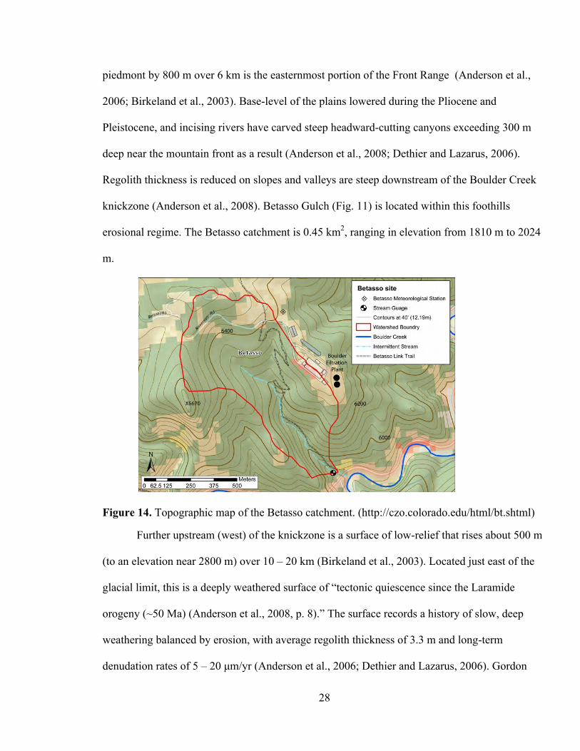
28
piedmont by 800 m over 6 km is the easternmost portion of the Front Range (Anderson et al.,
2006; Birkeland et al., 2003). Base-level of the plains lowered during the Pliocene and
Pleistocene, and incising rivers have carved steep headward-cutting canyons exceeding 300 m
deep near the mountain front as a result (Anderson et al., 2008; Dethier and Lazarus, 2006).
Regolith thickness is reduced on slopes and valleys are steep downstream of the Boulder Creek
knickzone (Anderson et al., 2008). Betasso Gulch (Fig. 11) is located within this foothills
erosional regime. The Betasso catchment is 0.45 km2, ranging in elevation from 1810 m to 2024
m.
Figure 14. Topographic map of the Betasso catchment. (http://czo.colorado.edu/html/bt.shtml)
Further upstream (west) of the knickzone is a surface of low-relief that rises about 500 m
(to an elevation near 2800 m) over 10 – 20 km (Birkeland et al., 2003). Located just east of the
glacial limit, this is a deeply weathered surface of “tectonic quiescence since the Laramide
orogeny (~50 Ma) (Anderson et al., 2008, p. 8).” The surface records a history of slow, deep
weathering balanced by erosion, with average regolith thickness of 3.3 m and long-term
denudation rates of 5 – 20 µm/yr (Anderson et al., 2006; Dethier and Lazarus, 2006). Gordon

29
Gulch is part of this low relief terrain. Gordon Gulch is 2.74 km2, ranging in elevation from 2446
m to 2737 m.
Figure 15. Topographic map of Gordon Gulch, Colorado (http://czo.colorado.edu/html/gg.shtml)
The final erosional regime in the Boulder Creek CZO is the alpine surface, where the
Front Range rises 1000 m over a distance of 10 – 15 km to the continental divide (Birkeland et
al., 2003). This zone consists of deep valleys with major steps and flats that were formed by
Pleistocene glaciers. Cirque basins lie at the head of these alpine valleys, just below the
Continental Divide (Anderson et al., 2006). The Green Lakes Valley (7.1 km2) (Fig. 16) is in this
alpine zone (Caine, 1995). Elevations range from 3200 m to 3745 m.

30
Figure 16. Topographic map of Green Lakes Valley, Colorado.
Geologic Background
The Laramide orogeny (~60 Ma) was the last major tectonic event affecting the Colorado
Front Range, resulting in uplift of the Rocky Mountains and driving the erosion that helped
expose modern Front Range geomorphology (Anderson et al., 2006). Precambrian basement
rocks of igneous and metamorphic origin underlie the Boulder Creek CZO. The most common
rock units are >1.7 Ga biotite and hornblende gneisses and metasediments, the 1.7 Ga Boulder
Creek Granodiorite and the 1.4 Ga Silver Plume granite (Gable, 1980). Small Tertiary dikes of
monzonite and quartz monzonite composition locally intrude the Proterozoic units (Birkeland et
al., 2003). Common minerals of these rock units are quartz, microcline, plagioclase, biotite, and
hornblende; alteration of primary minerals has yielded mixed layer smectite-illite, vermiculite,
chlorite, kaolinite, and short-range order/amorphous minerals (Dethier and Lazarus, 2006).

31
Climate and vegetation
Across the Boulder Creek catchment, temperature and precipitation vary widely due to
the large elevation gradient (>2.5 m). There are substantial seasonal variations in temperature as
well, a result of the continental climate regime. The strong climatic gradient of the Front Range
controls the distribution of vegetation zones within the catchment (Fig. 17).
Figure 17. Temperature, precipitation, and vegetation patterns in the Front Range. From Birkeland et al. (2003, modified from Veblen and Lorenz (1991)).
Betasso Gulch is in the lower montane climatic zone. Mean annual temperature is 10.0◦C
and mean precipitation is approximately 58 cm (Barry, 1973; Cowie, 2010). Maximum
precipitation occurs in May. Betasso Gulch is dominated by Ponderosa pine, with intermixed
Douglas fir on the north-facing slopes. In lower reaches of Betasso Gulch, slopes are steep and
regolith is commonly thin, with deeply weathered saprolite outcropping in places. The upper
reaches of Betasso Gulch are more gently sloping, and regolith is thicker than in the lower
reaches.

32
Gordon Gulch lies within the upper montane climatic zone. Mean annual temperature is
6.8◦C and mean precipitation is 58 cm (Barry, 1973; Cowie, 2010). Similar to Betasso Gulch,
maximum precipitation occurs in the month of May. In lower Gordon Gulch, the north-facing
slopes are much more densely vegetated than the south facing slopes. Lodgepole pine dominates,
especially on the north-facing slopes, and Douglas fir and Ponderosa pine are also present.
Ponderosa pines are more numerous on the south-facing slopes, where summer conditions are
drier and warmer. Near the stream in lower Gordon Gulch and in shallow sloping areas of upper
Gordon gulch are aspen groves and meadows.
The lower reaches of the Green Lakes Valley (GLV) are in the subalpine climatic zone
and below tree-line, but the upper reaches of the catchment reach the Continental Divide and
alpine tundra persists. Mean annual temperature in GLV is -3.7◦C and mean annual precipitation
is 93 cm (of which 80% is snow). Precipitation is greatest in March and January, and runoff
reaches a maximum in July (Caine, 1995). The lower portions of GLV are forested, dominated
by subalpine firs and Engelman spruce that progressively decrease in density with increasing
elevation (Birkeland et al., 2003). Above tree-line (~3400 m), alpine tundra vegetation covers
less than a third of the area; the remaining area is comprised of steep rock faces and talus slopes
(Caine, 1995).
Paleoclimate
The Front Range records a history of significant glaciation in the Pleistocene, most
clearly evidenced by deeply carved alpine valleys near the range crest. Moraine and till deposits
indicate the extent of these glaciations (Fig. 18), and cosmogenic radionuclide exposure dates
from Ward et al. (2009) show that the glaciation of Middle Boulder Creek valley reached a
maximum extent between ~22 ka to ~18 ka, with an ELA 600 m lower than the modern. Glacial

33
retreat was slow and proceeded episodically; the lower portions of the glaciers in Boulder Creek
(both North and Middle branches, nearly 2/3 of the glacier length) were deglaciated between 18
ka and 14 ka and the upper Green Lakes Valley was deglaciated rapidly between 15 ka and 13 ka
(Caine, 1995; Dühnforth and Anderson, 2011; Ward et al., 2009) (Caine, 1995; Ward et al.,
20099, Dühnforth and Anderson, 2011).
Figure 18. Lower limits of Pleistocene glaciation (~22 ka – 18 ka) in the Colorado Front Range, indicated by glacial deposits (dotted pattern). The gray pattern shows the modern surface of low relief. Approximate locations of Green Lakes Valley (GL), Gordon Gulch (GG), and Betasso Gulch (BG) shown in red. Modified from Birkeland (2003).
The extent and duration of Pleistocene glaciers suggest some combination of lower
temperatures and higher precipitation relative to modern conditions. Temperature estimates

34
range from 3◦C to 13◦C lower than today with precipitation increases between 0% and 100%
(Dühnforth and Anderson, 2011). Furthermore, during the late Pleistocene (~20 ka to 14 ka)
there was a high sediment supply due to glacial activity, and episodic sediment aggradation and
incision occurred in Boulder Canyon. Once glaciers retreated nearly completely (before 12 ka),
sediment supply was reduced and incision of the valley fill occurred; this incision continues
today, evidenced by the migration of knickpoints up Boulder Creek and tributary channels.
(Dühnforth and Anderson, 2011).
The consequence of the Pleistocene glaciation varies by location. On the floor of the
Green Lakes Valley, soils generally form from till, and formed less than 18 ka. Gordon Gulch is
just east of the glacial limit, and may preserve evidence of periglacial processes on the higher,
shallow sloping sites. Long-term valley incision has steepened slopes in lower Gordon Gulch,
and increased sediment transport. Betasso Gulch has responded similarly to Gordon Gulch to the
valley incision, with steeper slopes and thinner soils in the lower portion of the basin. Vegetation
zones across the study area have likely migrated to higher elevations since the late Pleistocene,
because of the warmer and drier climate Holocene climate.
Land-use history
Varied types of land-use disturb the landscapes in different ways, and potentially affect
soil formation and morphology due to denudation, compaction, and/or excavation of the land
surface. European settlement in the Front Range began in the late 1850’s and was primarily
driven by the potential for gold and silver in the Rockies (Veblen and Lorenz, 1991). After
settlement in Boulder and then Netherland, Gordon Gulch and Betasso were lightly forested for
timber and numerous prospector’s pits are scattered across the landscape in Gordon Gulch.

35
Today, only limited tree-cutting takes place by the USFS for fire prevention. Old forest service
roads and recreational paths are common in Gordon Gulch and Betasso. In the Green Lakes
Valley, a few remnant mining camps can be seen, but access is strictly limited and few roads and
paths exist in the valley. The roads in the valley were used to install small dams on the Green
Lakes to provide storage for the municipality of Boulder.
Purpose of Study
Based on field and laboratory analysis, this study seeks to (1) characterize weathering
patterns in high-relief environments by tracking the concentrations of pedogenic iron compounds
within and between soil profiles; and (2) assess the contributions and effects of eolian materials
on montane soils. Soil morphology, soil texture, and soil geochemistry will also be used to
evaluate weathering and soil development patterns in the study area. Geochemical analysis may
indicate eolian sedimentation and, furthermore, dust provenance. The varied topography of the
Colorado Front Range permits examination of soil development on hillslopes, and potentially
will yield information about the relationship between eolian sedimentation and hillslope position.
Pedogenic iron will also be employed in determining the relative ages of soils in the study area,
permitting assessment of landscape stability. Variance in soil development and eolian deposition
will be analyzed with respect to soil age, climate, and position in the landscape.

36
METHODS
In order to measure weathering and soil development and assess eolian contributions to
soils in the Boulder Creek catchment, I used a variety of field and laboratory methods. In the
field, I gave careful consideration to site selection, soil description parameters, and sampling
methods in order to: (1) have a representative and reliable sample suite; and (2) be able to
effectively relate field morphology to laboratory data. In the laboratory, various analyses permit
evaluation of soil development and dustfall. Specifically I sought to determine pedogenic iron
concentrations, texture, and geochemistry of the soil samples. Pedogenic iron is iron from
primary minerals that has been “released” by weathering and soil forming processes, and
represents the concentration of secondary iron oxides and organically bound iron complexes in a
soil. This iron is determined by a specific extraction technique using sodium-dithionite as the
principal reagent, and is thus known as Fed (McFadden and Hendricks, 1985).
Soil texture may indicate both weathering patterns and eolian enrichment of soils, as
eolian sediments are strongly fractionated by particle size. Soil geochemistry permits evaluation
of pedogenesis in soils, because it indicates the relative mobility of major and trace elemental
consituents throughout the soil column. Furthermore, soil geochemical analysis may help
quantify the amount of dustfall if the incoming sediment is geochemically distinct from the
underlying parent material.
Field
Site selection
I selected 24 sites in the Boulder Creek catchment for field description and sampling
(Fig. 19). The sites together represent varying elevation, slope, aspect, parent material, moisture
regime, and inferred age. Ease of access was also an important factor in site selection, so, when
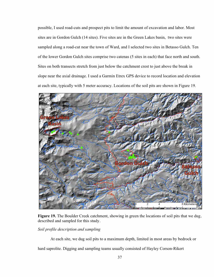
37
possible, I used road-cuts and prospect pits to limit the amount of excavation and labor. Most
sites are in Gordon Gulch (14 sites). Five sites are in the Green Lakes basin, two sites were
sampled along a road-cut near the town of Ward, and I selected two sites in Betasso Gulch. Ten
of the lower Gordon Gulch sites comprise two catenas (5 sites in each) that face north and south.
Sites on both transects stretch from just below the catchment crest to just above the break in
slope near the axial drainage. I used a Garmin Etrex GPS device to record location and elevation
at each site, typically with 5 meter accuracy. Locations of the soil pits are shown in Figure 19.
Figure 19. The Boulder Creek catchment, showing in green the locations of soil pits that we dug, described and sampled for this study.
Soil profile description and sampling
At each site, we dug soil pits to a maximum depth, limited in most areas by bedrock or
hard saprolite. Digging and sampling teams usually consisted of Hayley Corson-Rikert

38
(Wesleyan University), Ellie Maley (Smith College), Cianna Wyshnytzki (Amherst College) and
myself. We were advised and assisted by the project coordinator, Professor David Dethier
(Williams College). Surfaces where soil were described and sampled were approximately one
meter wide. I followed standard soil description procedures, noting horizons and their depths. I
primarily used soil color, soil texture (approximated by field tests) and clast abundance to
indentify and name horizons. I then labeled soil horizons with nails and flagging tape, and put a
tape measure in place before photographs were taken of each soil profile (Fig. 20).
I collected approximately 750 g of soil from all horizons (98 samples total), with the
exception of O and L horizons where present. I excluded large clasts (>2 cm), as future
laboratory analysis required using the <2 mm fraction of the regolith. In some locations, a single
horizon would be of significant thickness (usually >60 cm), and I would sample it at two
separate depths. I sampled in this matter because horizons that may appear visibly homogenous
across a large thickness may actually display marked changes in soil chemistry and texture. The
samples were collected in labeled “Ziploc” bags to preserve moisture content.
When sampling, I typically collected channel samples of each individual horizon. This is
not only because I wanted a soil sample that would represent the entire thickness of each
horizon, but also because the density of clasts in lower horizons made other methods (e.g.
interval sampling) impractical.
While in the field, I determined bulk density for a select number of horizons. I did this by
gently hammering a 250 ml metal cylinder into the face of the soil profile. To collect a relatively
undisturbed sample that preserves pore space. I then determined the weight of the soil with a
portable digital balance. The mass of the soil (in grams) divided by the volume of the cylinder
(250 cm3) yields a bulk density value in g cm-3.

39
Figure 20. Soil pit description and sampling at the Ward road-cut site. Pictured from left to right are Cianna Wyshnytzky (Amherst College), Ellie Maley (Smith College), and Hayley Corson-Rikert (Wesleyan University).
40
Laboratory
I carried out soil analyses in the Environmental Analysis Lab at Williams College, guided
by Jay Racela, the Technical Assistant.
Sample preparation and percent moisture
I dry-sieved all samples into >2 mm and <2 mm fractions using USDA standard soil
sieves. I placed the >2 mm portions in appropriately labeled bags for storage. I then weighed <2
mm samples individually, recording their weight using a Fisher-Scientific top-loading digital
balance accurate to 0.01g. To weigh the <2 mm samples, I poured each one into its own labeled
600 ml beaker after taring each beaker on the balance before soil was added and weighed.
I then placed the soil-filled beakers into a Precision brand mechanical convection oven,
and dried them at 80°C for at least 24 hours. After drying, I reweighed the soil. I then calculated
percent moisture for each sample using the wet and dry mass of the soil in the following
equation:
(eq. 3) Sample partitioning
After drying all of the <2 mm samples, I divided each sample into two subsamples for
further analysis. It was important that subsamples were well mixed. To help homogenize the
samples, I overturned and shook each many times before partitioning and divided them vertically
rather than horizontally, as some degree of sorting occurred even after agitation and thorough
mixing of the sample. Approximately 100g is required for grain size analysis using the
hydrometer method, so I made sure I had at least that much for every sample and placed it in a
%Moisture =wet soil mass(g) - dry soil mass(g)
wet soil mass(g)=
Mwater
Mtotal
41
new and appropriately labeled Ziploc bag. When I had excess soil, I saved 200 g for grain-size
analysis. This is done to evaluate the precision of the grain-size analyses.
For analysis of dithionite-extractable iron (Fed) and to prepare samples for elemental
analysis (conducted by Acme Analytical Laboratories), I separated the <150 µm fraction. Using
the remaining soil after 100 g had been put aside for grain size analysis, I manually sieved each
sample to 150 µm. The <2 mm, >150 µm samples were preserved in separate bags. The <150 µm
samples are generally of low mass, and I placed them into small glass vials to store in dessicating
cupboards while awaiting later analyses. I determined dry soil color of the <2 mm, >150 µm
fraction using the Munsell color system under natural light.
Selective dissolution analysis: dithionite-extractable iron (Fed)
Fed was determined by standard methods (Gee and Bauder, 1986; McFadden and
Hendricks, 1985). For each horizon I mixed 0.5 g of the <150 µm fraction with 30 ml of sodium
bicarbonate-sodium citrate buffer and 0.2 g of sodium-dithionite. I placed the samples in a water
bath at approximately 77˚C for 15 minutes, and then added 15 ml of distilled water to cool the
samples and centrifuged the samples for 10 minutes at 2000 rpm. The supernatant was removed
and put aside, and I extracted the solid sample again according to the procedure listed above.
After the second extraction, I combined the supernatant with the supernatant from the first
extraction and discarded the solid sample. I diluted the supernatant with distilled water to 100ml
and ran it through a Whatman paper filter. I then measured the iron concentration in each extract
using an atomic absorption spectrometer (AAS) (Fig. 21). To determine % dithionite-extractable
iron (Fed), I stoichiometrically converted %Fed to %Fe2O3.
I determined the mass of Fe2O3 in individual soil horizons by multiplying the
concentration of extractable Fe2O3 by the horizon thickness and bulk density. The sum of these

42
values from each horizon in a soil profile yields the total profile Fed content, as Fe2O3. Using
measured Fed concentrations from unweathered parent material horizons (Cu) or from bedrock
bulk chemistry (data obtained from D.P. Dethier), I established parent material values for Fed for
each site. I then calculated the mass of accumulated Fed, as Fe2O3 (in g cm-2) at each site by
subtracting the parent material mass of Fed (as Fe2O3) from the total mass of Fed (as Fe2O3). In
addition to the samples I collected, I also analyzed 14 samples from previous field studies in the
Front Range, including a profile formed in Bull Lake (130 ka) till and sampled by R. Shroba of
the U. S. Geological Survey.
Figure 21. Using the atomic absorption spectrometer (AAS) to analyze dithionite-extractable iron (Fed) in the Williams College Environmental Analysis Laboratory. Photograph by Jay Racela.
43
Soil texture
I measured soil texture by the hydrometer method (Gee and Bauder, 1986). I used
approximately 100 g samples of the <2 mm fraction for the analysis; these samples were
previously set aside during initial sample preparation (see above). I weighed each sample on the
Fisher-Scientific digital balance, and recorded that mass to 0.01 g accuracy. All samples were
~100 g ± 2.5%. I prepared samples by adding 10 ml of dilute Calgon solution (a
detergent/dispersant) and approximately 300 ml of deionized water. Samples were stirred and set
aside for 15 minutes and then mixed in mechanical mixers for 15 minutes to ensure adequate
dispersal and disaggregation of soil particles. An additional step was taken for preparation of A-
horizons. In order to accurately determine soil texture, organic matter had to first be removed. I
placed ~100 g samples in a beaker with 100 ml of distilled water, and 30 ml of 30% hydrogen
peroxide. I heated the samples on a hot plate to ensure that the hydrogen peroxide completely
oxidized the carbon in the sample. In some samples, I added more H2O2 to bring the reaction to
completion. Samples were removed from the beaker and allowed to settle for 24 hours at
minimum. I removed the residual liquid from the sample and then processed the solid sample
according to the procedure described above. Measurements were taken at 15, 30, 60, and 90
seconds and at 5, 20, 90, and 1440 minutes (24 hours).
Using equations from Gee and Bauder (1986), I used the hydrometer measurements
calculate the proportions of various size fractions; I determined percent sand, silt and clay.
Similar to the method used for Fed, I calculated total mass of clay in each horizon by
multiplying percent clay by bulk density (g cm-3) and horizon thickness (cm). I determined the
total profile clay content (in g cm-2) by adding together the mass of clay from each horizon in a
given profile.

44
Soil geochemical analysis
51 samples were sent to Acme Analytical Laboratories Ltd. For bulk geochemical
analysis. Abundances of major component oxides and trace elements were determined by ICP-
emission spectrometry and ICP-mass spectrometry, respectively. Samples in each analysis were
prepared by standard methods: Lithium metaborate / tetraborate fusion and dilute nitric acid
digestion. Loss on ignition (LOI) by mass was also determined.
46 samples sent for geochemical analysis are from a total of 9 soil profiles from this
study, located in Gordon Gulch, the Green Lakes valley, and the Ward road-cut site. 28 of these
represent pairs of coarse (>150µm) and fine (<150µm or <63µm) soil fractions from 14 soil
horizons; 12 of these samples are pairs of surface and parent material horizons from 6 profiles.
This sampling scheme permitted geochemical comparison of coarse and fine soil fractions, as
well as surface and subsurface soil horizons. 18 samples are <150 µm fractions of sequential soil
horizons from 4 profiles, permitting geochemical analysis of whole profiles. The remaining 5
samples (provided by D. P. Dethier) are from regolith collected in 2009 from exposed rootballs
(due to treefall) in Gordon Gulch. They serve as a source of comparison.

45
RESULTS Field measurements, laboratory data, and photographs from all study sites are presented
in Appendix A and Appendix B, while geochemical data is presented in Appendix C. The results
presented below summarize the data presented in this appendix.
Field Green Lakes Valley
Soils in the Green Lakes Valley formed from glacial till on stable slopes or periglacial
colluvium on the valley walls. Two sites (BCW_SLQ-01 and GL1-01) formed from Pinedale till
and exhibit strong horizonation. SLQ-01, at ~3200 m elevation, exhibits A/Ej/Bw/Cox/Cu
horizonation and the Cu is reached at 102 cm (Fig. 22). GL1-01, the highest soil sampled
(elevation 3550 m), is A/Bw/Cox/Cu; the A and B horizons are thinner (8 and 34 cm,
respectively) than SLQ-01, and the Cu horizon is reached at 70 cm depth. Soils in moist
meadows on higher-elevation colluvial slopes (BCW-01, BCW-02) are less well-developed and
have thick (~20 cm) A-horizons underlain by thick Bw horizons (~50cm); Cu horizons were not
reached at either site, but they likely consist of periglacial deposits. A soil on the Niwot Ridge
road (BCW-03) records a much more complex history of weathering, and a 120 cm A/B/Cox
sequence overlies a > 40 cm thick Btb.
Gordon Gulch In Gordon Gulch the two catenas are broadly similar at the shoulder and upper backslope,
but show marked differences near the footslope. All soils on the south-facing slope transect are
thin (<1 m) and have thin A horizons, underlain by Cox horizons that are progressively rockier
with depth, limiting the depth of pits. Hard saprolite horizons (Cr) were reached at SFT-01,
SFT-1B, and SFT-00. Soils along the north-facing slope transect are less than 1m deep and
weakly developed at the shoulder and upper backslope. These upper profiles (NFT-04 and NFT-
03) are comprised of thin (<10 cm) A and Bw horizons, underlain by Cox horizons that are

46
rockier with depth. At both of these upper slope sites, heavily jointed saprolite (Cr) was reached.
In contrast to the south-facing slope, soils thicken dramatically on the lower backslope of the
north-facing slope (175 cm and 188 cm), and have complex profiles consisting mostly of thick,
weakly weathered colluvium. A well-developed, stable soil of Pinedale age from the Green
Lakes valley, a thin backslope soil, and a thick colluvial footslope soil (Fig. 22) illustrate the
range of soils I analyzed.
Figure 22. Three soil profiles from the Boulder Creek CZO. SLQ-01 is a soil from the Green Lakes basin formed in Pinedale glacial till (~15 ka), reaching a depth of approximately 110 cm in the field of view. SFT-1B is a 68 cm-thick soil from the south-facing slope of lower Gordon Gulch (saprolite boundary at 38 cm). NFT-01 is a 188 cm-thick soil from the north-facing slope of Gordon Gulch.
Soils in upper and middle Gordon Gulch formed from saprolite at higher elevation on
shallower slopes than those in lower Gordon Gulch. At these sites, the saprolite-soil interface
occurs at less than 1 m depth. Bt horizons were noted at both upper Gordon sites (UGG-01 and

47
UGG-02). The middle Gordon Gulch soils (MGG-01 and MGG-02) formed from weathered
saprolite that is not seen in other portions of Gordon Gulch; at other sites, the saprolite is
typically overlain by a very blocky (clasts >10 cm) Cox horizon and the saprolite below is hard
and cohesive on the south-facing slope (Fig. 22). In middle Gordon Gulch, Cox horizons are thin
and have few large clasts in them, and the saprolite is much softer (Fig. 23).
Figure 23. A typical middle Gordon Gulch soil, MGG-02, with a deeply weathered saprolite (Cr) and thin Cox. The profile shown here is 115 cm deep. Note the preservation of the rock structure in the saprolite, indicated by the more and less-altered zones dipping parallel to the foliation (bounded by black dashed lines).
48
Betasso Gulch and Ward
Soils in the Betasso Gulch derive from either weathered colluvium derived from
weathered saprolite or the weathered saprolite, and both sites show thick (>50 cm) Bt horizons.
BTO-01 was dug to 145 cm and contains a thick, well preserved buried soil. The buried sequence
is Ab/Btb, thicker and more strongly developed than the modern soil. BTO-02 is A/Bt and was
dug to 108 cm. The Ward road-cut site is a long exposure (~100 m) that is >300 cm thick and is
the most deeply weathered site sampled in this study. It has complex morphology; the exposure
shows a channel that has been infilled and a well-defined periglacial ice-wedge. WRC-01 is a
soil profile that formed within the infilled channel, and is 283 cm deep with multiple buried soils.
Laboratory
Dithionite-extractable iron
Percent Fed varies considerably in my samples, which is expected due to the effects of
pedogenesis. BCW-01Bw yielded the highest concentration of Fed (as Fe2O3) at 3.12%.
BCW_SLQ-01Ej yielded the lowest concentration of Fed (as Fe2O3) at 0.56%. The mean
concentration of Fed as Fe2O3 is 1.74% (n = 120; 1 sigma = 0.613)
Total profile accumulated Fed (as Fe2O3) also varies significantly across the catchment,
with an average value of 1.84 g cm-2 and a standard deviation of 1.51 g cm-2. The maximum
value is 5.1 g cm-2 at the site “WRC-01”; the minimum accumulated Fe2O3 is 0.19 g cm-2 at the
site “SFT-03.” Using accumulated Fed from stable sites of known age, I calculated a Fed
accumulation rate; as expected, Fed correlates positively with age (Fig. 24).

49
Figure 24. Fed accumulation rate, determined by using total profile accumulated Fed content of four soils of known age. The soil from Betasso Gulch (red bullet) formed from deep, weathered colluvium and a substantial and uncertain portion of the Fe2O3 content is inherited. For this reason, the profile was not used to fit the curve. See Appendix A for complete profile descriptions.
Stable sites are those that have not significantly eroded or aggraded during soil formation
and display clear relations between overlying soil horizons and display clear relations to the
parent material. GL1-01 and BCW_SLQ-01 formed from till of Pindale age and thus are
constrained to an age ~15 ka. UGG-02 was determined by optically-stimulated luminescence
(OSL) to have formed 26 ka (J. Völkel, personal correspondence). GRL-328 formed in Bull Lake
till (~130 ka).
Soil texture

50
Textural results show that all horizons at all sites classify as either sandy loam, loamy
sand, or sand on the USDA texture diagram (Birkeland, 1999). Average concentrations of sand,
silt, and clay (n = 100) are 81.5%, 14.5%, and 5.1%, respectively. I calculated proportions of
four size fractions within the silt range (50 µm – 2 µm): a coarse fraction (50 µm >x> 22 µm), a
medium fraction (22µm>x>11µm), a fine fraction (11µm>x>5.5µm), and a very fine fraction
(5.5 µm >x> 2 µm). These finer fractions permit more specific evaluation of silt, and may help
discriminate between silt-sized particles released by weathering and finer silt-sized particles that
are eolian in origin. The <11 µm fraction (i.e. %clay + %fine silt + %very fine silt) is reported in
the following analyses because it represents the size range expected for distant eolian sediment
sources.
Total profile clay content correlates strongly with total profile Fed content (exponential
R2 = 0.81), and a strong positive correlation between accumulated clay content and accumulated
Fed content exists as well (exponential R2 = 0.87) (Fig. 25 and 26).
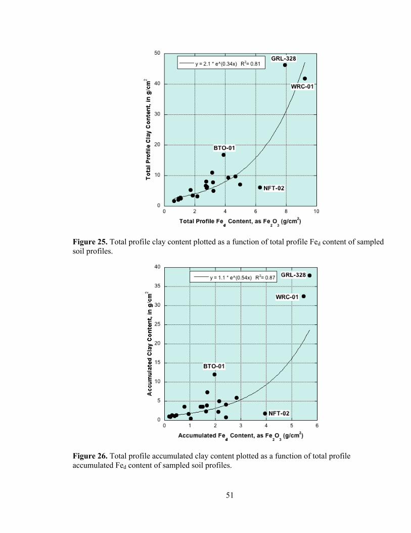
51
Figure 25. Total profile clay content plotted as a function of total profile Fed content of sampled soil profiles.
Figure 26. Total profile accumulated clay content plotted as a function of total profile accumulated Fed content of sampled soil profiles.
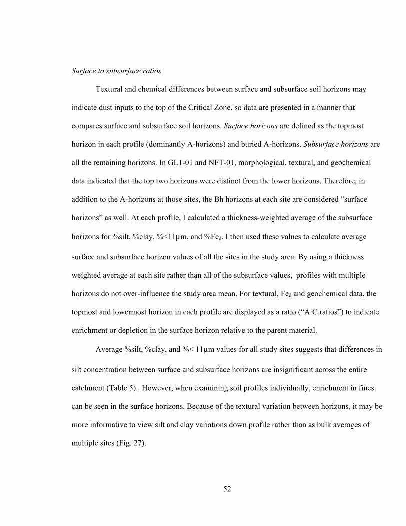
52
Surface to subsurface ratios
Textural and chemical differences between surface and subsurface soil horizons may
indicate dust inputs to the top of the Critical Zone, so data are presented in a manner that
compares surface and subsurface soil horizons. Surface horizons are defined as the topmost
horizon in each profile (dominantly A-horizons) and buried A-horizons. Subsurface horizons are
all the remaining horizons. In GL1-01 and NFT-01, morphological, textural, and geochemical
data indicated that the top two horizons were distinct from the lower horizons. Therefore, in
addition to the A-horizons at those sites, the Bh horizons at each site are considered “surface
horizons” as well. At each profile, I calculated a thickness-weighted average of the subsurface
horizons for %silt, %clay, %<11µm, and %Fed. I then used these values to calculate average
surface and subsurface horizon values of all the sites in the study area. By using a thickness
weighted average at each site rather than all of the subsurface values, profiles with multiple
horizons do not over-influence the study area mean. For textural, Fed and geochemical data, the
topmost and lowermost horizon in each profile are displayed as a ratio (“A:C ratios”) to indicate
enrichment or depletion in the surface horizon relative to the parent material.
Average %silt, %clay, and %< 11µm values for all study sites suggests that differences in
silt concentration between surface and subsurface horizons are insignificant across the entire
catchment (Table 5). However, when examining soil profiles individually, enrichment in fines
can be seen in the surface horizons. Because of the textural variation between horizons, it may be
more informative to view silt and clay variations down profile rather than as bulk averages of
multiple sites (Fig. 27).
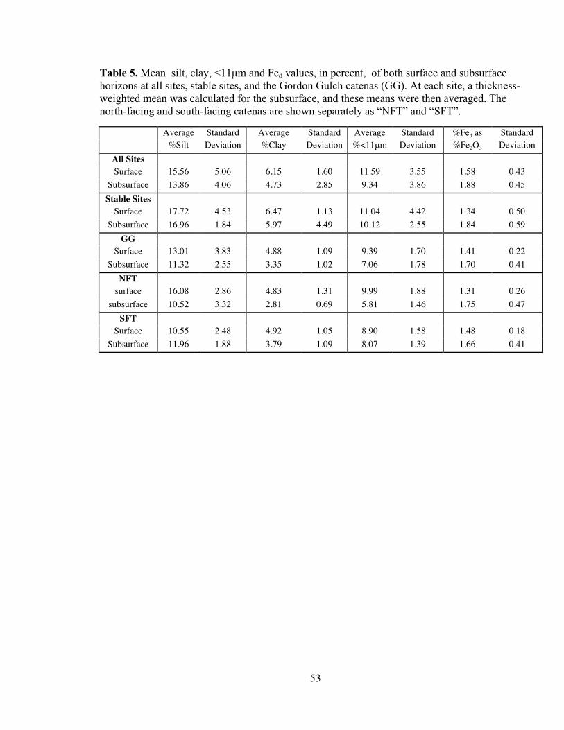
53
Table 5. Mean silt, clay, <11µm and Fed values, in percent, of both surface and subsurface horizons at all sites, stable sites, and the Gordon Gulch catenas (GG). At each site, a thickness-weighted mean was calculated for the subsurface, and these means were then averaged. The north-facing and south-facing catenas are shown separately as “NFT” and “SFT”.
Average Standard Average Standard Average Standard %Fed as Standard %Silt Deviation %Clay Deviation %<11μm Deviation %Fe2O3 Deviation
All Sites Surface 15.56 5.06 6.15 1.60 11.59 3.55 1.58 0.43
Subsurface 13.86 4.06 4.73 2.85 9.34 3.86 1.88 0.45 Stable Sites
Surface 17.72 4.53 6.47 1.13 11.04 4.42 1.34 0.50 Subsurface 16.96 1.84 5.97 4.49 10.12 2.55 1.84 0.59
GG Transects
Surface 13.01 3.83 4.88 1.09 9.39 1.70 1.41 0.22
Subsurface 11.32 2.55 3.35 1.02 7.06 1.78 1.70 0.41 NFT
surface 16.08 2.86 4.83 1.31 9.99 1.88 1.31 0.26 subsurface 10.52 3.32 2.81 0.69 5.81 1.46 1.75 0.47
SFT Surface 10.55 2.48 4.92 1.05 8.90 1.58 1.48 0.18
Subsurface 11.96 1.88 3.79 1.09 8.07 1.39 1.66 0.41

54
Figure 27. Diagram of NFT-03, displaying concentrations of Fed and fine particles (<11 µm) down profile. The A and Bw horizons are enriched in fine particles.
Dithionite-extractable iron (Fed), as %Fe2O3, is generally lower in surface horizons than
subsurface horizons (Table 5); this relationship persists throughout the catchment. A:C horizon
ratios also indicate lower Fed in the surface than in the parent material (Table 6). At stable sites,
however, A:C of Fed is 1.19. This likely represents a difference in parent material; most of the
stable sites form from till, and Cu horizons were sampled at these sites. In soils that form from
crystalline bedrock, stony Cox horizons or dense saprolite limited the depth of pits, and we never
exposed the weathering front. That is, the parent material on hillslopes is oxidized. For that
reason, Fed is lower in C-horizons at the stable sites.

55
Table 6. Mean A-horizon to C-horizon ratios of percent silt, clay, <11µm fraction, and Fed at all site, stable sites, and Gordon Gulch (GG). The north-facing catena (NFT) and south-facing catena (SFT) are shown separately as well. 1 sigma (STDEV) is also shown.
A : C ratios Silt Clay (<11um) Fed All Sites 1.32 1.76 1.55 0.90 STDEV 0.79 1.12 0.98 0.34
Stable Sites 0.91 1.99 1.08 1.19 STDEV 0.15 2.04 0.61 0.71
GG Transects
1.53 1.74 1.69 0.80 STDEV 1.04 0.75 0.67 0.18
NFT 2.16 2.00 2.24 0.70 STDEV 1.13 0.72 0.38 0.19
SFT 1.03 1.54 1.26 0.87 STDEV 0.70 0.78 0.49 0.14
Soil Geochemistry
Bulk geochemical analyses are reported in Appendix C. After correcting for LOI, surface
to subsurface horizon ratios (A:C) of major oxides follow expected patterns (Birkeland, 1999);
Silica is slightly enriched in surface horizons (mean = 1.11; 1 sigma = 0.06), whereas Al, Fe, and
K are depleted (Table 7). Na, Ca, Mg, and P are slightly depleted in surface horizons on average,
but vary widely. High field strength elements (HFSE) and rare-earth elements (REE) are
typically depleted in surface horizons relative to the subsurface, but values deviate widely
between profiles (Table 8, Table 9, Table 10). UGG-02 is notable because it records low A:C
values for HFSE and REE, and distribution of major oxides through the soil column differs
greatly from the general patterns observed in the study area. The lowest horizon at UGG-02 is a
Crt with very high %Fed (3.8% as Fe2O3), suggesting that illuviation of mobile consituents
occurs in the Crt.
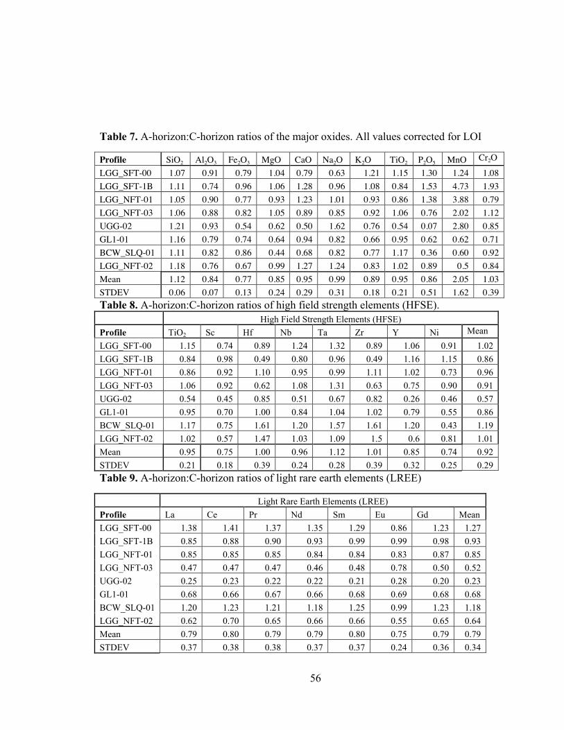
56
Table 7. A-horizon:C-horizon ratios of the major oxides. All values corrected for LOI
Profile SiO2 Al2O3 Fe2O3 MgO CaO Na2O K2O TiO2 P2O5 MnO Cr2O3 LGG_SFT-00 1.07 0.91 0.79 1.04 0.79 0.63 1.21 1.15 1.30 1.24 1.08
LGG_SFT-1B 1.11 0.74 0.96 1.06 1.28 0.96 1.08 0.84 1.53 4.73 1.93 LGG_NFT-01 1.05 0.90 0.77 0.93 1.23 1.01 0.93 0.86 1.38 3.88 0.79 LGG_NFT-03 1.06 0.88 0.82 1.05 0.89 0.85 0.92 1.06 0.76 2.02 1.12 UGG-02 1.21 0.93 0.54 0.62 0.50 1.62 0.76 0.54 0.07 2.80 0.85 GL1-01 1.16 0.79 0.74 0.64 0.94 0.82 0.66 0.95 0.62 0.62 0.71 BCW_SLQ-01 1.11 0.82 0.86 0.44 0.68 0.82 0.77 1.17 0.36 0.60 0.92 LGG_NFT-02 1.18 0.76 0.67 0.99 1.27 1.24 0.83 1.02 0.89 0.5 0.84 Mean 1.12 0.84 0.77 0.85 0.95 0.99 0.89 0.95 0.86 2.05 1.03 STDEV 0.06 0.07 0.13 0.24 0.29 0.31 0.18 0.21 0.51 1.62 0.39 Table 8. A-horizon:C-horizon ratios of high field strength elements (HFSE). High Field Strength Elements (HFSE) Profile TiO2 Sc Hf Nb Ta Zr Y Ni Mean
LGG_SFT-00 1.15 0.74 0.89 1.24 1.32 0.89 1.06 0.91 1.02 LGG_SFT-1B 0.84 0.98 0.49 0.80 0.96 0.49 1.16 1.15 0.86 LGG_NFT-01 0.86 0.92 1.10 0.95 0.99 1.11 1.02 0.73 0.96 LGG_NFT-03 1.06 0.92 0.62 1.08 1.31 0.63 0.75 0.90 0.91 UGG-02 0.54 0.45 0.85 0.51 0.67 0.82 0.26 0.46 0.57 GL1-01 0.95 0.70 1.00 0.84 1.04 1.02 0.79 0.55 0.86 BCW_SLQ-01 1.17 0.75 1.61 1.20 1.57 1.61 1.20 0.43 1.19 LGG_NFT-02 1.02 0.57 1.47 1.03 1.09 1.5 0.6 0.81 1.01 Mean 0.95 0.75 1.00 0.96 1.12 1.01 0.85 0.74 0.92 STDEV 0.21 0.18 0.39 0.24 0.28 0.39 0.32 0.25 0.29 Table 9. A-horizon:C-horizon ratios of light rare earth elements (LREE)
Light Rare Earth Elements (LREE) Profile La Ce Pr Nd Sm Eu Gd Mean LGG_SFT-00 1.38 1.41 1.37 1.35 1.29 0.86 1.23 1.27 LGG_SFT-1B 0.85 0.88 0.90 0.93 0.99 0.99 0.98 0.93 LGG_NFT-01 0.85 0.85 0.85 0.84 0.84 0.83 0.87 0.85 LGG_NFT-03 0.47 0.47 0.47 0.46 0.48 0.78 0.50 0.52 UGG-02 0.25 0.23 0.22 0.22 0.21 0.28 0.20 0.23 GL1-01 0.68 0.66 0.67 0.66 0.68 0.69 0.68 0.68 BCW_SLQ-01 1.20 1.23 1.21 1.18 1.25 0.99 1.23 1.18 LGG_NFT-02 0.62 0.70 0.65 0.66 0.66 0.55 0.65 0.64 Mean 0.79 0.80 0.79 0.79 0.80 0.75 0.79 0.79 STDEV 0.37 0.38 0.38 0.37 0.37 0.24 0.36 0.34
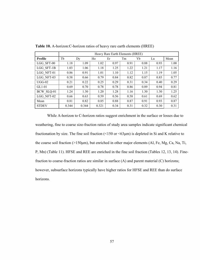
57
Table 10. A-horizon:C-horizon ratios of heavy rare earth elements (HREE)
Heavy Rare Earth Elements (HREE) Profile Tb Dy Ho Er Tm Yb Lu Mean LGG_SFT-00 1.18 1.09 1.02 0.97 0.91 0.88 0.93 1.00 LGG_SFT-1B 1.03 1.06 1.18 1.25 1.22 1.21 1.17 1.16 LGG_NFT-01 0.86 0.91 1.01 1.10 1.12 1.15 1.19 1.05 LGG_NFT-03 0.58 0.66 0.79 0.84 0.82 0.87 0.85 0.77 UGG-02 0.21 0.22 0.25 0.29 0.31 0.34 0.40 0.29 GL1-01 0.69 0.70 0.78 0.78 0.86 0.89 0.94 0.81 BCW_SLQ-01 1.24 1.30 1.20 1.28 1.16 1.30 1.30 1.25 LGG_NFT-02 0.66 0.63 0.59 0.56 0.58 0.61 0.69 0.62 Mean 0.81 0.82 0.85 0.88 0.87 0.91 0.93 0.87 STDEV 0.344 0.344 0.321 0.34 0.31 0.32 0.30 0.31
While A-horizon to C-horizon ratios suggest enrichment in the surface or losses due to
weathering, fine to coarse size-fraction ratios of study area samples indicate significant chemical
fractionation by size. The fine soil fraction (<150 or <63µm) is depleted in Si and K relative to
the coarse soil fraction (>150µm), but enriched in other major elements (Al, Fe, Mg, Ca, Na, Ti,
P, Mn) (Table 11). HFSE and REE are enriched in the fine soil fraction (Tables 12, 13, 14). Fine-
fraction to coarse-fraction ratios are similar in surface (A) and parent material (C) horizons;
however, subsurface horizons typically have higher ratios for HFSE and REE than do surface
horizons.

58
Table 11. Fine-fraction to coarse-fraction ratios of the major oxides. Mean values of all sites, surface horizons, and subsurface horizons are provided. “Subsurface” here denotes parent material (C) horizons.
Major Oxides Sample Name SiO2 Al2O3 Fe2O3 MgO CaO Na2O K2O TiO2 P2O5 MnO Cr2O3 LGG_SFT-00A 0.90 1.32 1.17 1.53 1.51 1.02 0.85 1.45 1.64 1.25 0.46 LGG_SFT-00Cr2 0.77 1.88 1.76 2.02 1.30 1.24 1.68 1.85 2.65 1.23 0.51 LGG_SFT-1B_A 0.89 1.29 1.52 1.88 1.59 1.11 0.83 1.68 1.91 1.94 3.95 LGG_SFT-1B_Cr 0.79 1.81 1.44 1.49 1.37 1.25 0.88 1.76 1.91 0.69 0.46 LGG_NFT-01A 0.92 1.22 1.42 1.68 1.57 1.19 0.84 1.63 1.54 1.42 2.25 LGG_NFT-02C1 0.85 1.59 1.55 1.63 1.05 1.06 0.96 1.72 1.66 1.04 0.52 LGG_NFT-02C5 0.80 1.66 1.26 1.21 1.61 1.05 0.95 1.23 1.55 0.69 1.79 LGG_NFT-03ABw 0.94 1.27 1.32 1.88 1.11 0.99 0.73 2.01 1.32 0.82 0.38 LGG_NFT-03Cr 0.95 1.25 1.16 1.12 0.92 0.93 0.70 1.20 1.54 1.03 1.85 UGG-02A 0.94 1.22 1.06 1.62 2.13 1.01 0.81 1.28 1.55 1.75 0.36 UGG-02Crt 0.93 1.09 0.96 0.96 3.43 0.89 0.98 0.96 3.36 1.01 1.09 GL1-01A 0.94 1.13 1.72 1.83 1.31 0.79 0.66 1.88 1.76 1.83 0.24 GL1-01Cu 0.83 1.38 1.98 2.31 1.03 0.82 1.09 1.85 1.90 1.88 1.92 BCW-SLQ-01A 0.97 1.06 1.35 1.38 0.99 0.91 0.85 1.33 1.61 1.02 0.41
Mean 0.89 1.37 1.40 1.61 1.50 1.02 0.91 1.56 1.85 1.26 1.16 1 Sigma 0.07 0.26 0.29 0.37 0.65 0.14 0.25 0.32 0.54 0.44 1.07
Mean Surface 0.93 1.22 1.36 1.69 1.35 1.00 0.79 1.61 1.62 1.43 1.15 1 Sigma 0.02 0.09 0.20 0.18 0.23 0.12 0.07 0.25 0.17 0.39 1.31
Mean Subsurface 0.85 1.52 1.44 1.54 1.21 1.03 1.03 1.51 2.08 1.08 1.16 1 Sigma 0.07 0.29 0.36 0.49 0.87 0.17 0.31 0.37 0.68 0.40 0.68
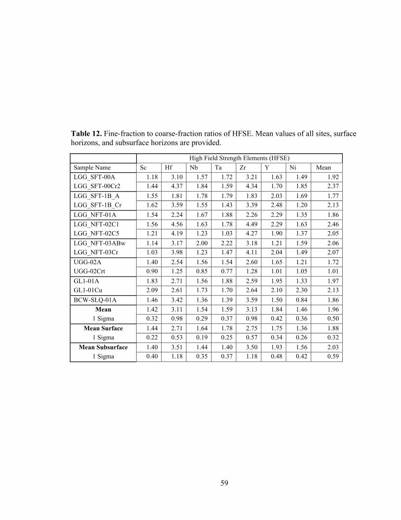
59
Table 12. Fine-fraction to coarse-fraction ratios of HFSE. Mean values of all sites, surface horizons, and subsurface horizons are provided.
High Field Strength Elements (HFSE) Sample Name Sc Hf Nb Ta Zr Y Ni Mean LGG_SFT-00A 1.18 3.10 1.57 1.72 3.21 1.63 1.49 1.92 LGG_SFT-00Cr2 1.44 4.37 1.84 1.59 4.34 1.70 1.85 2.37 LGG_SFT-1B_A 1.55 1.81 1.78 1.79 1.83 2.03 1.69 1.77 LGG_SFT-1B_Cr 1.62 3.59 1.55 1.43 3.39 2.48 1.20 2.13 LGG_NFT-01A 1.54 2.24 1.67 1.88 2.26 2.29 1.35 1.86 LGG_NFT-02C1 1.56 4.56 1.63 1.78 4.49 2.29 1.63 2.46 LGG_NFT-02C5 1.21 4.19 1.23 1.03 4.27 1.90 1.37 2.05 LGG_NFT-03ABw 1.14 3.17 2.00 2.22 3.18 1.21 1.59 2.06 LGG_NFT-03Cr 1.03 3.98 1.23 1.47 4.11 2.04 1.49 2.07 UGG-02A 1.40 2.54 1.56 1.54 2.60 1.65 1.21 1.72 UGG-02Crt 0.90 1.25 0.85 0.77 1.28 1.01 1.05 1.01 GL1-01A 1.83 2.71 1.56 1.88 2.59 1.95 1.33 1.97 GL1-01Cu 2.09 2.61 1.73 1.70 2.64 2.10 2.30 2.13 BCW-SLQ-01A 1.46 3.42 1.36 1.39 3.59 1.50 0.84 1.86
Mean 1.42 3.11 1.54 1.59 3.13 1.84 1.46 1.96 1 Sigma 0.32 0.98 0.29 0.37 0.98 0.42 0.36 0.50
Mean Surface 1.44 2.71 1.64 1.78 2.75 1.75 1.36 1.88 1 Sigma 0.22 0.53 0.19 0.25 0.57 0.34 0.26 0.32
Mean Subsurface 1.40 3.51 1.44 1.40 3.50 1.93 1.56 2.03 1 Sigma 0.40 1.18 0.35 0.37 1.18 0.48 0.42 0.59

60
Table 13. Fine-fraction to coarse-fraction ratios of LREE. Mean values of all sites, surface horizons, and subsurface horizons are provided.
Light Rare Earth Elements (LREE) Sample Name La Ce Pr Nd Sm Eu Gd Mean LGG_SFT-00A 1.96 1.90 1.91 1.96 1.88 1.44 1.90 1.85 LGG_SFT-00Cr2 2.70 2.61 2.71 2.73 2.67 2.09 2.62 2.59 LGG_SFT-1B_A 2.20 2.23 2.21 2.25 2.17 1.50 2.16 2.10 LGG_SFT-1B_Cr 2.56 2.57 2.57 2.56 2.51 1.65 2.54 2.42 LGG_NFT-01A 2.01 2.04 2.03 1.86 1.97 1.26 1.94 1.88 LGG_NFT-02C1 2.35 2.36 2.33 2.40 2.31 1.23 2.23 2.17 LGG_NFT-02C5 2.18 2.13 2.12 2.20 2.14 1.75 2.09 2.09 LGG_NFT-03ABw 1.57 1.57 1.58 1.57 1.59 1.05 1.55 1.50 LGG_NFT-03Cr 1.94 1.95 1.93 2.00 1.95 1.09 2.07 1.85 UGG-02A 2.06 2.01 1.99 2.07 1.91 1.88 1.85 1.97 UGG-02Crt 1.58 1.58 1.61 1.64 1.53 1.94 1.41 1.61 GL1-01A 1.56 1.55 1.50 1.51 1.54 1.37 1.74 1.54 GL1-01Cu 2.05 2.13 2.06 2.03 1.99 1.64 2.04 1.99 BCW-SLQ-01A 2.16 2.19 2.00 1.86 1.84 1.42 1.81 1.90
Mean 2.06 2.06 2.04 2.04 2.00 1.52 2.00 1.96 1 Sigma 0.34 0.34 0.35 0.36 0.34 0.32 0.34 0.31
Mean Surface 1.93 1.93 1.89 1.87 1.84 1.42 1.85 1.86 1 Sigma 0.24 0.25 0.24 0.24 0.20 0.23 0.17 0.24
Mean Subsurface 2.19 2.19 2.19 2.22 2.16 1.63 2.14 2.09 1 Sigma 0.38 0.36 0.38 0.37 0.38 0.36 0.40 0.36

61
Table 14. Fine-fraction to coarse-fraction ratios of HREE. Mean values of all sites, surface horizons, and subsurface horizons are provided.
Heavy Rare Earth Elements (HREE) Sample Name Tb Dy Ho Er Tm Yb Lu Mean
LGG_SFT-00A 1.86 1.77 1.61 1.52 1.48 1.48 1.61 1.62 LGG_SFT-00Cr2 2.30 1.95 1.71 1.56 1.42 1.48 1.48 1.70 LGG_SFT-1B_A 2.12 2.11 2.03 2.02 1.87 1.94 1.92 2.00 LGG_SFT-1B_Cr 2.52 2.58 2.40 2.22 2.12 2.11 2.12 2.30 LGG_NFT-01A 2.07 2.18 2.12 2.20 2.22 2.09 2.24 2.16 LGG_NFT-02C1 2.29 2.25 2.32 2.27 2.26 2.39 2.52 2.33 LGG_NFT-02C5 2.04 1.96 2.07 2.07 1.90 1.92 2.02 2.00 LGG_NFT-03ABw 1.49 1.35 1.28 1.12 1.19 1.24 1.21 1.27 LGG_NFT-03Cr 2.04 2.04 1.86 1.83 2.02 1.94 2.09 1.97 UGG-02A 1.74 1.68 1.61 1.65 1.66 1.63 1.77 1.68 UGG-02Crt 1.28 1.18 1.05 0.97 0.93 0.91 0.88 1.03 GL1-01A 1.77 1.76 2.02 1.93 2.20 2.32 2.31 2.05 GL1-01Cu 2.06 2.13 2.19 2.35 2.30 2.32 2.28 2.23 BCW-SLQ-01A 1.68 1.64 1.56 1.54 1.38 1.53 1.57 1.56
Mean 1.95 1.90 1.84 1.80 1.78 1.81 1.86 1.85 1 Sigma 0.33 0.37 0.39 0.43 0.44 0.44 0.46 0.39
Mean Surface 1.82 1.78 1.75 1.71 1.71 1.75 1.80 1.83 1 Sigma 0.20 0.26 0.29 0.34 0.37 0.35 0.36 0.36
Mean Subsurface 2.08 2.01 1.94 1.89 1.85 1.87 1.91 1.87 1 Sigma 0.39 0.43 0.46 0.49 0.50 0.52 0.55 0.47

62
DISCUSSION
Introduction
Weathering patterns
Data collected in this study permit evaluation of weathering and dustfall rates in the
Boulder Creek catchment. Soils in this study form from stable sites, active slopes, and sites that
were mobile in the past (likely due to periglacial processes) that have since stabilized. This
variation permits evaluation of weathering rates with respect to regolith transport. Soil
morphology, Fed, texture and geochemistry indicate the transport and deposition of physical and
chemical constituents both downprofile and downslope. Variations along these physical and
chemical pathways primarily reflect gradients in precipitation, parent material, soil stability (i.e.
transport rate) and dustfall rate among my study sites. The precipitation gradient is controlled
strongly by elevation, and soils in GLV generally have stronger horizonation than those in
Gordon Gulch or Betasso Gulch. Soil parent materials range from Pinedale till and periglacial
slope deposits in GLV, to saprolite and weathered colluvium in GG and BG. That some GLV
parent materials are stable likely contributes to enhanced translocation of soil constituents, and
contributes to the strong horizonation observed there. Stable sites in the study area demonstrate
that Fed and clay accumulate downprofile with time in soils. In soils forming from mobile
regolith, clay and Fed also accumulate with time, but mixing of the soil column leads to more
uniform distributions of Fed and clay downprofile.
Soil parent material is closely related to soil stability on slopes, as the movement of
regolith downslope leads to the formation of cumulative soils at toeslope positions. Toeslope
soils record complex histories, and the presence of buried soils suggests that slope movement is
episodic in the study area. Soils at shoulder and backslope positions are well-mixed as a result of

63
this transport, and show weak horizonation. Overall in GG, soils are thinner, weakly developed
and likely younger because they are travelling downslope and mixing. At more stable positions,
transport rates are sufficiently low that pedogenic horizonation is well-preserved, and Bt
horizons develop.
Evidence for eolian deposition
In the study area, distinguishing between eolian and native soil components is difficult, in
part because soil/regolith is well mixed during weathering processes and downslope transport.
Furthermore, eolian sedimentation may be episodic, and deposition rates are sufficiently low that
pedogenesis is primarily influenced by the underlying parent material. However, eolian
sedimentation is recorded by analyzing Fed and clay concentrations through the soil column.
Although total profile Fed and clay content are positively correlated in the study area, surface
horizons, relative to subsurface horizons, are commonly enriched in clay and fine silt but
depleted in Fed. Enrichment of clay and silt, with low concentrations of Fed suggests eolian
enrichment of soils in the study area. Surface horizons are also enriched in rare-earth (REE) and
high field-strength (HFSE) elements, thus supporting the textural evidence for dustfall in the
catchment. The integration of eolian sediments with native sediments and size fractionation of
HFSE and REE, however, means that HFSE and REE concentrations in soils cannot be used
simply to determine eolian provenance.
In the Front Range, eolian silt mantles are observed in alpine environments (Dahms,
1993; Litaor, 1987; Muhs and Benedict, 2006). The strongest evidence of eolian deposition in
this study is from the alpine GLV, due to site stability. In the montane zones, however, results
from this study show that eolian sedimentation is occurring, and geochemistry suggests that
eolian sediments in the alpine are of similar provenance to eolian sediments in GG and BG. At

64
older sites (>20 kyr; WRC-01 and BCW-03), eolian materials have been translocated into the
subsurface, and soil textural and chemical patterns downprofile are dominantly pedogenic, but
likely influenced by parent material inputs from below (bedrock) and above (e.g. dust). That is,
the effect of eolian additions is less clear than at the young, stable sites.
Field relationships
Green Lakes valley
Two sites in the Green Lakes Valley (GL1-01 and SLQ-01) expose soils that have formed
out of Pinedale till, and are <15 kyr in age. Although the soils are young, they exhibit strong
horizonation, with <10 cm A-horizons and deep B horizons (34 and 51 cm, respectively),
reflecting both site stability and high precipitation. The presence of an Ej horizon at SLQ-01 and
not GL1-01 is likely due to lower soil pH (4.8 v. 5.11; H. Corson-Rikert thesis, 2011) generated
by the decomposition of coniferous vegetation; GL1-01 is above tree-line.
Both profiles show enrichment of fine sediments and low Fed in the surface. At SLQ-01,
Fed and clay show similar patterns in the subsurface, suggesting that clays in the subsurface are
primarily pedogenic. High clay and low Fed in the A-horizon indicates that the surface sediment
is distinct (Fig. 28). At GL1-01, the concentration of fines is much greater in the surface than in
the underlying horizons (Fig. 29). Fines (<11 µm) are at a minimum in the Bw horizon, where
Fed is at a maximum. This may appear partly due to the weathering and transport of Fed prior to
formation and mobility of clay minerals; however, the concentration of fine silts also mirrors this
change. Correlation between silt and clay-sized particles suggests that the clay bulge in the A-
horizon is not pedogenic in origin. Thus, textural data at both sites indicate eolian enrichment.

65
Figure 28. Clay and Fed concentrations at BCW_SLQ-01. Individual soil horizons are labeled.
Figure 29. Concentration of fine particles (<11 µm) and Fed at GL1-01. Individual soil horizons are labeled.

66
Textural evidence for eolian enrichment in the alpine is also supported by geochemical
data. At SLQ-01, the surface is enriched, relative to the subsurface, in REE and HFSE (Fig. 30).
At this site A-horizon to Cu-horizon ratios for all REE but Eu (0.99) are greater than 1, with an
average value of 1.22 (1 sigma = 0.08). Enrichment of HFSE is highest in Zr, but also occurs in
Hf, Nb, Ta, Y, and Ti. Depletion of Ni and Sc (0.43 and 0.75, respectively) is also observed.
Figure 30. Concentrations of Zr, Y (x 10), Ce, and Ti at BCW_SLQ-01. Soil horizons are labeled.
Sites BCW-01 and BCW-02 have mixed, ~20 cm thick A-horizons underlain by >50 cm
thick B-horizons, with similar accumulated Fed values to GL1-01 and SLQ-01. Thicker, mixed
A-horizons at BCW-01 and BCW-02 (see Appendix A) are likely a result of physical mixing due
to downslope transport, as these two sites are located on the valley walls rather than the shallow
valley floor. Located above the Pinedale ice limit (K. Kantack thesis, 2011), BCW-01 and BCW-
02 are potentially of greater age than the valley floor soils. However, it is difficult to accurately
predict age based upon accumulated Fed because of downslope transport. That is, accumulated
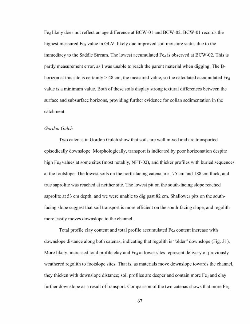
67
Fed likely does not reflect an age difference at BCW-01 and BCW-02. BCW-01 records the
highest measured Fed value in GLV, likely due improved soil moisture status due to the
immediacy to the Saddle Stream. The lowest accumulated Fed is observed at BCW-02. This is
partly measurement error, as I was unable to reach the parent material when digging. The B-
horizon at this site is certainly > 48 cm, the measured value, so the calculated accumulated Fed
value is a minimum value. Both of these soils display strong textural differences between the
surface and subsurface horizons, providing further evidence for eolian sedimentation in the
catchment.
Gordon Gulch
Two catenas in Gordon Gulch show that soils are well mixed and are transported
episodically downslope. Morphologically, transport is indicated by poor horizonation despite
high Fed values at some sites (most notably, NFT-02), and thicker profiles with buried sequences
at the footslope. The lowest soils on the north-facing catena are 175 cm and 188 cm thick, and
true saprolite was reached at neither site. The lowest pit on the south-facing slope reached
saprolite at 53 cm depth, and we were unable to dig past 82 cm. Shallower pits on the south-
facing slope suggest that soil transport is more efficient on the south-facing slope, and regolith
more easily moves downslope to the channel.
Total profile clay content and total profile accumulated Fed content increase with
downslope distance along both catenas, indicating that regolith is “older” downslope (Fig. 31).
More likely, increased total profile clay and Fed at lower sites represent delivery of previously
weathered regolith to footslope sites. That is, as materials move downslope towards the channel,
they thicken with downslope distance; soil profiles are deeper and contain more Fed and clay
further downslope as a result of transport. Comparison of the two catenas shows that more Fed
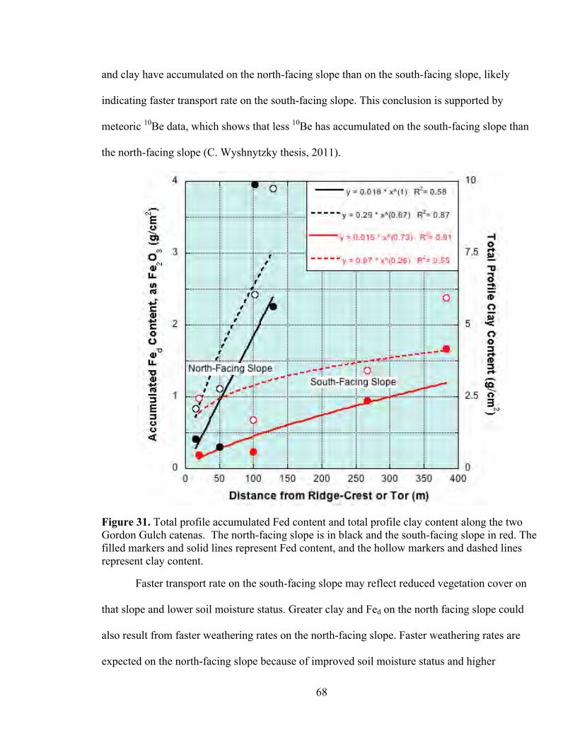
68
and clay have accumulated on the north-facing slope than on the south-facing slope, likely
indicating faster transport rate on the south-facing slope. This conclusion is supported by
meteoric 10Be data, which shows that less 10Be has accumulated on the south-facing slope than
the north-facing slope (C. Wyshnytzky thesis, 2011).
Figure 31. Total profile accumulated Fed content and total profile clay content along the two Gordon Gulch catenas. The north-facing slope is in black and the south-facing slope in red. The filled markers and solid lines represent Fed content, and the hollow markers and dashed lines represent clay content.
Faster transport rate on the south-facing slope may reflect reduced vegetation cover on
that slope and lower soil moisture status. Greater clay and Fed on the north facing slope could
also result from faster weathering rates on the north-facing slope. Faster weathering rates are
expected on the north-facing slope because of improved soil moisture status and higher

69
vegetation density. As expected, when comparing backslope sites from the north-facing and
south-facing slope, pH was found to be lower on the north-facing slope (pH = 5.18 and 5.5,
respectively).
Evidence for eolian sedimentation along the Gordon Gulch catenas is complicated by
downslope transport and mixing. On the north-facing slope, surface enrichment in fines is
greatest at the lowest site, NFT-01, and is also observed at NFT-02 and NFT-03 (Fig. 32). Fed is
lower in the surface horizons relative to the subsurface horizons at these sites, suggesting that
this fine material is eolian. At NFT-01, however, the surface horizon geochemistry does not
uniformly display enrichment in HFSE and REE. This is likely due to the fact that the deepest
horizon that was sampled for geochemical analysis at NFT-01 has a maximum depth of 69 cm,
but the total profile reaches a depth of 188 cm. The lower horizon (Coxb), similar to the A at this
site, likely contains transported material from upslope and has been well mixed. Because of this
mixing, eolian sedimentation is not clearly indicated by differences in HFSE and REE
concentrations between the A and Coxb.

70
Figure 32. Concentration of fine particles (<11 µm) and Fed at NFT-01. Individual soil horizons are labeled.
Soils on the south-facing slope show only slight enrichment of the surface horizons in
fine particles. The average concentration of fines (<11 µm) in the surface, Cox, and Cr horizons
on the south-facing slope are 8.90%, 8.54%, and 7.88%, respectively. On the north-facing slope,
average concentration of fines in the surface and subsurface horizons are 10.51% and 5.95%,
respectively. The differences between the north and south-facing slopes suggests that soils are
less-efficiently mixed on the north-facing slope. The average total profile mass of fines on the
north-facing slope is 10.4 g/cm2; average total profile mass of fines on the south-facing slope
(including Cr horizons, therefore, it is a maximum estimate) is 7.5 g cm-2. The average mass
reflects accumulation of fines due to both weathering and dust accumulation. That this mass is
higher on north-facing slopes again indicates greater transport rate on the south-facing slope.
Higher mass of fines on the north-facing slope, which is shorter and transported more slowly
71
than the south-facing, indicates that fines from the south-facing slope are being transported from
the system, and not accumulating at the foot of the slope. These fines accumulate in alluvial fans
and terraces along the axial drainage, or are transported out of Gordon Gulch by the stream.
Sites in upper and middle GG are more stable than the lower GG catenas, and are less
influenced by transport and mixing. Both middle GG sites are enriched in surface fines. At upper
GG, soils are well developed and form from deeply weathered saprolite. At UGG-02, the
formation and/or incorporation of clays in buried Bt horizons controls the distribution of fines in
the soil column, and both textural and geochemical evidence for eolian enrichment of the surface
horizons are weak. However, eolian sedimentation is likely occurring here because other
locations in GG record a strong eolian signature.
Betasso Gulch, Ward, and BCW-03
The two soils in Betasso gulch are distinct from other soils in the study area because they
exhibit thick (>50cm) Bt horizons. Despite the high clay concentrations in the subsurface due to
pedogenesis, fines are enriched in the surface at BTO-02, suggesting that eolian deposition also
occurs in BG. BTO-01 is forming out of colluvium, and a thick buried sequence suggests
episodic transport at this site. There is little surface enrichment of fines, likely due to mixing
from transport, but the total profile mass of fines is very high.
The Ward road-cut site (WRC-01) and BCW-03 record deep weathering histories, and
are above the Pinedale glacial limit. The presence of an ice-wedge cast at WRC-01 suggests that
periglacial mass movement processes operated on these slopes. Both soils record deep buried Bt
horizons and high Fed accumulation. Accumulated Fed values at WRC-01 and BCW-03 suggest
ages of 109 kyr and 27.3 kyr, respectively. The difference in age between WRC-01 and BCW-03
is significant, as evidence of eolian sedimentation is increasingly muted with increased

72
pedogenesis. At WRC-01, correlative clay and Fed concentrations through the soil profile
indicate that clays are likely pedogenic in origin, or have been incorporated into the soil by
pedogenesis. That is, clay enrichment is not observed in the surface (Fig. 33). At BCW-03, Fed
and fines are correlated in the subsurface, but the surface shows significant enrichment of fines
(Fig. 34). This indicates that, although horizonation is strong in the subsurface, surface fines
have not yet been mixed and incorporated into the soil column.
Figure 33. Concentration of clay and Fed at WRC-01. Individual soil horizons are labeled. Note the strong correlation between clay and Fed.

73
Figure 34. Concentration of fine particles (<11 µm) and Fed at BCW-03.
Establishing weathering and dustfall rates
Fed and clay accumulate with increasing age at stable sites in the study area (Figure 35).
However, clay enrichment in the surface horizons of soils typically is not matched by Fed
enrichment. For this reason, I have argued that a portion of clay enrichment in the surface is not
due to pedogenesis, but is the result of eolian additions to the surface. This conclusion is
supported by surface enrichment in fine silt particles that mirrors enrichment in clay.

74
Figure 35. Total profile clay and Fed accumulation rate, determined using soils of known age. Soil profiles are labeled.
Ferrier et al. (2011) calculated a long-term dustfall rate of 0.3 to 1.3 g cm-2 kyr-1 for semi-arid
soils in Idaho, which equates to 30 g to 130 g of dustfall per 100 kyr. In the Colorado Plateau,
dustfall rates are higher, but have decreased from 3.47 g cm-2 kyr-1 in the middle Holocene to a
modern rate of 1.04 g cm-2 kyr-1 (Reynolds et al., 2006a). On San Clemente Island in southern
California, estimated dust flux ranges from 0.865 g cm-2 kyr-1 to 3.5 g cm-2 kyr-1 (Muhs et al.,
2007b). Dust composition varies significantly between the above mentioned studies, indicating
different dust source areas.
Figure 35 shows that, at 100 kyr, soils in the Boulder Creek catchment will have
accumulated approximately 30 g of clay, supplied by dustfall and weathering. If the
accumulation rate proposed by Ferrier et al. (2011) applies to the Boulder Creek catchment, all
of the clay in study area soils could have originated as dustfall. In my study, I defined dust-sized

75
particles as the <11 µm fraction, and the clay fraction (<2 µm) averages approximately 49% of
the <11 µm fraction by mass. Therefore, if 30 g of clay were supplied by dust, an additional 30 g
of fine silt-sized dust would also fall, and a total of ~60 g of dust could accumulate in 100 kyr.
However, a portion of the dust-sized particles in my study sites is likely produced in situ. At this
point, the proportion of clay-sized and silt-sized particles that originate as from dust, relative to
the proportion produced by in situ weathering, is poorly constrained by my data. Therefore,
precise dust accumulation rates cannot yet be determined in the study area. With a maximum
dustfall rate of 60 g per 100 kyr in the study area, which improbably assumes no in situ
production of clay and fine-silt, it is likely that that the dustfall rate in the Boulder Creek
catchment is at or below the lower limit of the dustfall rate determined by Ferrier et al. (2011).
Using Figure 35, one can also evaluate the mass of Fed that could potentially originate
from dust. The average Fed measured in this study is 1.7% (n = 114) and the maximum is 3.8%.
In a study of dustfall in the Colorado Plateau and the American Southwest, dust contained
between 4.4 and 2.6 percent Fe2O3 (Reheis et al., 2002). If one assumes that, over 100 kyr, the 60
g of clay-sized dust deposited contained at maximum 5% Fed as Fe2O3, then 3.0 g of Fed would
accumulate; however, this is a maximum estimate, because the amount of dust falling over 100
kyr is likely less than 60 g and its Fed concentration is likely less than 5%. Using the Fed
accumulation rate from Figure 35, approximately 5.1 g of Fed as Fe2O3 will accumulate over 100
kyr in soils in the study area. This suggests that, at maximum, 60% of the Fed in the study area is
from dust deposition. That is, more than 40% of the Fed in study area soils is produced in situ.
Even though 40% is a minimum estimate for the proportion of Fed produced in situ, it
demonstrates that a significant portion of the Fed in the study area is due to weathering.

76
The production of Fed resulting from weathering is particularly well demonstrated at
stable sites in the study area, where weathering and dustfall rates can be evaluated because soils
are less efficiently mixed and there is little regolith delivery from upslope. Chemical differences
in the soil profile at stable sites primarily result from in situ weathering, pedogenic translocation
and eolian sedimentation because physical transport is limited. At SLQ-01, geochemical data
suggest that a maximum of half of the accumulated Fed in the B-horizon is produced in situ; the
remainder is translocated from the A and E horizons above. I determined this by using the
concentration of Fe2O3 from both the parent material (Cu) and the B-horizons to determine the
mass of Fe2O3 accumulated from above. I then subtracted that value from the mass of
accumulated Fed in the B-horizons, with the difference representing the mass of Fed produced in
situ. The following relationship was used for these calculations:
Fetotal = thickness x density x concentration
Table 15. Select data from SLQ-01 that was employed to determine the amount of Fed produced in situ and translocated from above.
Horizon Thickness (cm) Density g cm-3 %Fe2O3 Acc. Fed (g cm-2) A 9 1.5 7.08 -0.018 E 6 1.7 6.6 -0.016
Bw 17 2 9.63 0.738 Bw2 16 2 9.88 0.468 Bw3 18 2 7.54 0.168 Cu - 2 8.26 -
The calculations indicated that 0.72 g Fe2O3 were transported to the B-horizons from above and
0.65 g of Fed accumulated from in situ weathering. This approach assumes that the concentration
of Fe2O3 in the Cu-horizon is equal to the initial concentration of Fe2O3 in the B-horizons (i.e.
when first deposited). Similar concentrations of Fe2O3 in the Cox horizon and similar Fed
concentrations for the Cu samples taken at 205 and 305 cm indicate that the parent material is

77
relatively homogenous. Operating under the same assumption, I determined the amount of the
Fed lost in the A and Ej horizons by subtracting the mass of Fe2O3 in the A and E-horizons from
an equivalent thickness of soil that has parent material (Cu) density and Fe2O3 concentration.
This calculation is counter to my previous argument, in that it assumes no Fed is accumulating in
the surface due to dustfall. This approach also assumes that the modern A-thickness is
representative, and significant denudation has not occurred. The result indicates that
approximately 0.85 g of Fe2O3 were lost from the A-horizon and Ej-horizons, which is similar to
the calculated gain of Fe2O3 in the B-horizons from above (0.72 g), indicating that the
preservation of mass is reasonably maintained in these calculations. The slight discrepancy in the
two values is likely due to the fact that bulk density values used in these calculations are
estimated values and were not measured in the field. The preservation of mass of Fe2O3 between
the surface (A + Ej) and B-horizons suggests that incoming dust is of low Fed and/or low
accumulation rate.
Evaluating dust provenance
Trace element concentrations may indicate the source and amount of dustfall in an area,
but precise determination is difficult. This is because dust can be both local and far-traveled in
origin, and dust chemistry may reflect multiple upwind sources and therefore be non-unique.
While trace-element ratios may not precisely indicate the dust source in the study area, they do
provide sound evidence of eolian enrichment. In the absence of dustfall of different composition,
weathering at SLQ-01 should yield similar A to Cu-horizon ratios for Ti and Zr. At SLQ-01,
however, A:Cu values for Ti and A:C values for Zr are 1.17 and 1.61, respectively, indicating
preferential enrichment in Zr, which suggests a dust source that is depleted in Ti relative to Zr.
The differences between Zr and Ti are not likely due to size fractionation. Although Zr is more
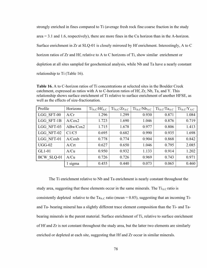
78
strongly enriched in fines compared to Ti (average fresh rock fine:coarse fraction in the study
area = 3.1 and 1.6, respectively), there are more fines in the Cu horizon than in the A-horizon.
Surface enrichment in Zr at SLQ-01 is closely mirrored by Hf enrichment. Interestingly, A to C
horizon ratios of Zr and Hf, relative to A to C horizons of Ti, show similar enrichment or
depletion at all sites sampled for geochemical analysis, while Nb and Ta have a nearly constant
relationship to Ti (Table 16).
Table 16. A to C-horizon ratios of Ti concentrations at selected sites in the Boulder Creek catchment, expressed as ratios with A to C-horizon ratios of Hf, Zr, Nb, Ta, and Y. This relationship shows surface enrichment of Ti relative to surface enrichment of another HFSE, as well as the effects of size-fractionation.
Profile Horizons TiA:C/HfA:C TiA:C/ZrA:C TiA:C/NbA:C TiA:C/TaA:C TiA:C/YA:C LGG_SFT-00 A/Cr 1.296 1.299 0.930 0.871 1.084 LGG_SFT-1B A/Cox2 1.723 1.690 1.046 0.876 0.719 LGG_NFT-03 ABw/Cox2 1.715 1.678 0.977 0.806 1.413 LGG_NFT-02 C1/C5 0.695 0.682 0.990 0.935 1.698 LGG_NFT-01 A/Coxb 0.778 0.774 0.904 0.868 0.842 UGG-02 A/Crt 0.627 0.650 1.046 0.795 2.085 GL1-01 A/Cu 0.950 0.932 1.133 0.914 1.202 BCW_SLQ-01 A/Cu 0.726 0.726 0.969 0.743 0.971 1 sigma 0.455 0.440 0.073 0.065 0.460
The Ti enrichment relative to Nb and Ta enrichment is nearly constant throughout the
study area, suggesting that these elements occur in the same minerals. The TiA:C ratio is
consistently depleted relative to the TaA:C ratio (mean = 0.85), suggesting that an incoming Ti-
and Ta- bearing mineral has a slightly different trace element composition than the Ti- and Ta-
bearing minerals in the parent material. Surface enrichment of Ti, relative to surface enrichment
of Hf and Zr is not constant throughout the study area, but the latter two elements are similarly
enriched or depleted at each site, suggesting that Hf and Zr occur in similar minerals.

79
Select trace element ratios have been used previously in the Front Range by Muhs and
Benedict (2006) to suggest origin of dust. When soils from my study area are plotted with those
of Muhs and Benedict, ratios from the fine fraction from A-horizons in the Boulder Creek
catchment fall between the biotite gneiss and granitic compositional fields (Fig. 36).
Figure 36. Ratios of Ti/Zr plotted against Ti/Nb from Muhs and Benedict (2006). Compositional fields of gneissic and granitic units of the Indian Peaks and Boulder Creek areas are shown. Hollow markers are the silt fraction of surface horizons collected by Muhs and Benedict (2006) in the Indian Peaks wilderness area, Colorado Front Range. Solid black markers are the fine fraction (<150 µm or <63 µm) of surface horizons from this study. The red and green markers represent the average composition (n=10 for each) of the fine fractions of Boulder Creek Granodiorite (BCG) and Silver Plume Granite (SPG), respectively. BCG and SPG samples were collected in the Boulder Creek catchment and analyzed by D.P. Dethier.
Figure 36 demonstrates that trace-element ratios from surface soils from this study are of similar
composition to silt mantles observed in the greater Indian Peaks region, which therefore suggests
a similar dust source. Muhs and Benedict (2006) argued that although the composition of silt
mantles is intermediate compared to the metasedimentary and granitic fields, it is likely derived

80
from a unique source because the compositional range of these silts is smaller than the range
observed in the two bedrock types. Muhs and Benedict (2006) also indicated with geochemical
data that two semi-arid basins northwest of the study area, North Park and Middle Park, are
likely sources of the eolian silts in Front Range soils. Soils from my study area are of similar
composition to those sampled by Muhs and Benedict (2006), indicating that fines in the Boulder
Creek catchment may also originate in North Park and Middle Park.
The dominant parent rocks for the unconsolidated sediment of North Park and Middle
Park are similar to the parent rocks in the study area; the composition of silt-sized alluvium in
these two basins reflects these bedrock units. Therefore, the differences in immobile element
compositions between the silt-sized alluvium and bedrock units shown in Figure 36 partially
reflect the influence of size-fractionation. Geochemical analysis of the fine (<250 µm) and
coarse (>250 µm) fractions of fresh BCG and SPG indicate that Zr and Nb are preferentially
enriched relative to Ti in the fine-fraction, and BCG fines plot within the compositional field of
the North Park and Middle Park alluvium. Therefore, fine soils from my study area may derive
from the weathering of underlying or nearby bedrock units. It is likely, however, that dustfall is
contributing a significant portion of these fine sediments, because surface horizons are enriched
in fines and low in Fed, indicating that a portion of the fines are not pedogenic in origin.
81
CONCLUSIONS
Soil texture, Fed, and geochemical data permit evaluation of the degree of weathering,
downslope transport, and eolian sedimentation in the Boulder Creek catchment. Soils in the
study area are varied, and morphology is often controlled by the degree of mixing that has
occurred at a given site. Stable soils form in areas of low topographic relief and show the
strongest horizonation. Mixed sites, as expected, are observed on steep slopes and are thinnest at
the summit and shoulder of hillslopes. Some sites were likely mobile in the glacial past due to
periglacial processes and are now more stable in the Holocene climate.
The two catenas in Gordon Gulch reveal that soils are thin, poorly developed, and well
mixed on the slope shoulder and upper backslope. Further downslope in Gordon Gulch, soil
morphology is complicated and north-facing slopes reach thicknesses >150 cm. Buried soil
horizons at NFT-01 suggest episodic transport of regolith to that toeslope. However, on the
south-facing slope of Gordon Gulch, soils downslope are not significantly thicker than soils
further upslope. Comparison of the two catenas shows that more Fed and clay have accumulated
on the north-facing slope than on the south-facing slope, likely indicating faster transport rate on
the south-facing slope. This conclusion is supported by meteoric 10Be data, which shows that less
10Be has accumulated on the south-facing slope than the north-facing slope (C. Wyshnytzky
thesis, 2011). The mass of fine silt and clay-sized particles on either slope reflects accumulation
of fines due to both weathering and dust accumulation and is greater on the north-facing slope,
again indicating greater transport rate on the south-facing slope. The south-facing slope in
Gordon Gulch shows little textural variation between surface and subsurface-horizons, which
suggests that soils are more-efficiently mixed on that slope than the north-facing slope, which
more clearly exhibits surface enrichment in fines.
82
Enrichment of fine particles and low Fed concentrations in the surface horizons of soils
indicates eolian sedimentation in the Boulder Creek catchment. Enrichment in HFSE and REE in
the surface supports the textural data. Eolian enrichment is most clearly demonstrated at stable
alpine sites of Pinedale age. In previous studies, eolian enrichment of alpine soils in GLV and
nearby areas has been observed by textural, geochemical and mineralogical means (Dahms,
1993; Litaor, 1987; Muhs and Benedict, 2006). On unstable and meta-stable sites on slopes, the
eolian component is well mixed in soils and evidence for eolian sedimentation is less clear than
at stable sites, though it is observed. Evidence for eolian sedimentation is increasingly muted
with increased pedogenesis, as eolian materials are incorporated into the soil and translocated to
B-horizons. In soils >20 kyr in age, fines are most concentrated in the B-horizons, and textural
evidence alone cannot indicate dustfall. However, HFSE and REE may be enriched.
Clay accumulation rate indicates that maximum dustfall rate in the catchment is 60 g cm-2
100kyr-1, but the actual accumulation rate is poorly constrained. Calculated Fed accumulation
rate and maximum dustfall rate indicate that >40% of the Fed in study area soils is produced in
situ by weathering processes. The actual portion of Fed produced in situ is likely much higher
than 40%, because this approach assumes that no clay and silt particles have accumulated due to
weathering and that all of it has fallen as dust.
Selected trace-element ratios show strong agreement with a study by Muhs and Benedict
(2006) in the Indian Peaks wilderness area, and suggest that surface fines in the Boulder Creek
catchment are eolian in origin. Similar Ti/Zr and Ti/Nb ratios are observed in surface horizons of
soils from my study area and elsewhere in the Indian Peaks region, suggesting a similar eolian
source. Due to size-fractionation of immobile elements in common bedrock units in the Front
Range, an exact source of this dust cannot be determined; However, a potential source of this

83
dust is alluvium from North Park and Middle Park, two semi-arid basins that are located west of
the continental divide (Muhs and Benedict, 2006).
Future work will include detailed comparison of data collected from this study and 10Be
data collected from many of the same sites by Cianna Wyshnytzky of Amherst College. This
hopefully will constrain the age of soils across the catchment more accurately, and allow for
determination of weathering, transport and dustfall rates. The soils at the Ward road-cut site
(WRC-01) and Niwot Ridge road (BCW-03) represent meta-stable sites that were more strongly
transported in the glacial past, and formed on a surface of low relief that has not yet been
significantly denuded due to migration of the Boulder Creek knickpoint upstream. Upper Gordon
Gulch soils also form from this surface, and anomalous geochemical data at UGG-02 has yet to
be resolved. Catena studies along this low-relief surface, similar to what was conducted in lower
GG, may better constrain the geomorphic history of these landforms. Specifically, catenas on the
Niwot Ridge nose and in upper GG are of interest. More work on dust chemistry and mineralogy
is always desirable, and long-term dust collectors will help to yield modern dust accumulation
rate and provenance data.

84
References Cited Anderson, R. S., and Anderson, S. P., 2010, Geomorphology: the mechanics and chemistry of
landscapes, Cambridge, Cambridge University Press, 637 p.: Anderson, R. S., Riihimaki, C. A., Safran, E. B., and MacGregor, K. R., 2006, Facing reality:
Late Cenozoic evolution of smooth peaks, glacially ornamented valleys, and deep river gorges of Colorado's Front Range: Geological Society of America, v. 398, p. 397-418.
Anderson, S. P., Bales, R. C., and Duffy, C. J., 2008, Critical Zone Observatories: Building a network to advance interdisciplinary study of Earth surface processes: Mineralogical Magazine, v. 72, no. 1, p. 7-10.
Anderson, S. P., von Blanckenburg, F., and White, A. F., 2007, Physical and chemical controls on the Critical Zone: Elements, v. 3, no. 5, p. 315-319.
Barber, L. B., Murphy, S. F., Verplanck, P. L., Sandstrom, M. W., Taylor, H. E., and Furlong, E. T., 2006, Chemical loading into surface water along a hydrological, biogeochemical, and land use gradient: A holistic watershed approach: Environmental Science & Technology, v. 40, no. 2, p. 475-486.
Barry, R. G., 1973, a climatological transect on the east slope of the Front Range, Colorado: Arctic and Alpine Research, v. 5, no. 2, p. 89-110.
Birkeland, P. W., 1999, Soils and Geomorphology, New York, Oxford University Press, 430 p. Birkeland, P. W., Shroba, R. R., Burns, S. F., Price, A. B., and Tonkin, P. J., 2003, Integrating
soils and geomorphology in mountains - an example from the Front Range of Colorado: Geomorphology, v. 55, p. 329-344.
Brantley, S. L., 2008, Understanding soil time: Science, v. 321, p. 1454-1455. Caine, N., 1995, Snowpack Influences on Geomorphic Processes in Green Lakes Valley,
Colorado Front Range: The Geographical Journal, v. 161, no. 1, p. 55-68. Cowie, R., 2010, The hydrology of headwater catchments from the plains to the continental
divide, Boulder Creek watershed, Colorado (MA thesis) [M.Sc.: University of Colorado, 122 p.
Dahms, D., 1993, Mineralogical evidence for eolian contribution to soils of late Quaternary moraines, Wind River Mountains, Wyoming, USA: Geoderma, v. 59, no. 1-4, p. 175-196.
Dethier, D. P., and Lazarus, E. D., 2006, Geomorphic inferences from regolith thickness, chemical denudation and CRN erosion rates near the glacial limit, Boulder Creek catchment and vicinity, Colorado: Geomorphology, v. 75, p. 384 - 399.
Dühnforth, M., and Anderson, R. S., 2011, in review, Reconstructing the glacial history of Green Lakes Valley, North Boulder Creek, Front Range, Colorado, using 10Be exposure dating: Arctic Alpine Antarctic Research.
Ferrier, K. L., Kirchner, J. W., and Finkel, R. C., 2011, in review, Estimating millenial-scale dust deposition rates on soil-mantled hillslopes using cosmogenic nuclides and immobile weathering tracers: Arctic Alpine Antarctic Research.
Gable, D. J., 1980, The Boulder Creek Batholith, Front Range, Colorado: U. S. Geol. Surv. Prof. Pap. , v. 1101, p. 88.
Gee, G. W., and Bauder, J. W., 1986, Particle-size analysis, in Klute, A., ed., Methods of soil analysis, Part 1. Agronomy Monograph 9: Madison, WI, ASA and SSSA, p. 383-411.

85
Heimsath, A. M., Dietrich, W. E., Nishiizumi, K., and Finkel, R. C., 1997, The soil production function and landscape equilibrium: Nature, v. 388, p. 358-361.
Heimsath, A. M., Dietrich, W. E., Nishiizumi, K., and Finkel, R. C., 1999, Cosmogenic nuclides, topography, and the spatial variation of soil depth: Geomorphology, v. 27, no. 1-2, p. 151-172.
Jenny, H., 1941, Factors of Soil Formation: A system of quantitative pedology, New York, McGraw-Hill Book Company.
Jenny, H., 1980, The Soil Resource, New York, Springer-Verlag, Ecological Studies. Jungers, M. C., Bierman, P. R., Matmon, A., Nichols, K., Larsen, J., and Finkel, R., 2009,
Tracing hillslope sediment production and transport with in situ and meteoric 10Be: Journal of Geophysical Research, v. 114, no. F4, p. 1-16.
Litaor, M. I., 1987, The influence of eolian dust on the genesis of alpine soils in the Front Range, Colorado: SSSAJ, v. 51, p. 142-147.
Mason, J. A., and Jacobs, P. M., 1998, Chemical and particle-size evidence for addition of fine dust to soils of the midwestern United States: Geology, v. 26, no. 12, p. 1135-1138.
McFadden, L. D., and Hendricks, D. M., 1985, Changes in the content and composition of pedogenic iron oxyhydroxides in a chronosequence of soils in Southern California: Quaternary Research, v. 23, p. 189-204.
McLaren, R. G., and Cameron, K. C., 1996, Soil science: sustainable production and environmental protection, Melbourne, Oxford Univeristy Press, 304 p.:
McLennan, S. M., 1989, Rare earth elements in sedimentary rocks: Influence of provenance and sedimentary processes: Reviews in Mineralogy, v. 21, p. 169-200.
Muhs, D. R., and Benedict, J. B., 2006, Eolian additions to Late Quaternary alpine soils, Indian Peaks Wilderness Area, Colorado Front Range: Artic, Antarctic, and Alpine Research, v. 38, no. 1, p. 120-130.
Muhs, D. R., and Budahn, J. R., 2006, Geochemical evidence for the origin of late Quaternary loess in central Alaska: Canadian Journal of Earth Science, v. 43, p. 323-337.
Muhs, D. R., Budahn, J. R., Johnson, D. L., Reheis, M., Beann, J., Skipp, G., Fisher, E., and Jones, J. A., 2008, geochemical evidence for airborne dust additions to soils in Channel Islands National Park, California: Geological Society of America Bulletin, v. January/February.
Muhs, D. R., Budahn, J. R., Prospero, J. M., and Carey, S. N., 2007a, Geochemical evidence for African dust inputs to soils of western Atlantic islands: Barbados, the Bahamas, and Florida: Journal of Geophysical Research, v. 112, no. F2, p. 1-26.
Muhs, D. R., Budahn, J. R., Reheis, M., Beann, J., Skipp, G., and Fisher, E., 2007b, Airborne dust transport to the eastern Pacific Ocean off southern California: Evidence from San Clemente Island: Journal of Geophysical Research, v. 112, no. D13203, p. 1-17.
Pye, K., 1987, Aeolian dust and dust deposits, London, Academic Press, Inc., 334 p. Raymond, L. A., 2002, Petrology: The study of igneous, sedimentary, and metamorphic rocks,
Long Grove, IL, Waveland Press, Inc. Reheis, M., Budahn, J. R., and Lamothe, P. J., 2002, Geochemical evidence for diversity of dust
sources in the southwestern United States: Geochemica et Cosmochimica Acta, v. 66, no. 9, p. 1569-1587.
Reynolds, R. L., Reheis, M., Neff, J. C., Goldstein, H., and Yount, J., 2006a, Late Quaternary eolian dust in surficial deposits of a Colorado Plateau grassland: Controls on distribution and ecologic effects: Catena, v. 66, p. 251-266.

86
Reynolds, R. L., Reheis, M., Yount, J., and Lamothe, P., 2006b, Composition of aeolian dust in natural traps on isolated surfaces of the central Mojave Desert - insights to mixing, sources, and nutrient inputs Journal of Arid Environments, v. 66, p. 42-61.
Schaetzl, R. J., and Anderson, S., 2005, Soils: genesis and geomorphology, New York, Cambridge University Press, 817 p.
Veblen, T. T., and Lorenz, D. C., 1991, The Colorado Front Range: a century of ecological change. , Salt Lake City, Univ. Utah Press, 186 p.:
Ward, D. J., Anderson, R. S., Guido, Z. S., and Briner, J. P., 2009, Numerical modeling of cosmogenic deglaciation records, Front Range and San Juan mountains, Colorado: Journal of Geophysical Research, v. 114, no. F01026, p. 1-21.
Yaalon, D. H., and Ganor, E., 1973, the influence of dust on soils during the Quaternary: Soil Science, v. 116, no. 3, p. 146-155.
87
APPENDIX A: Soil profile descriptions and photographs
Gordon Gulch soils: NFT-01, NFT-02, NFT-03, NFT-04, NFT-05, SFT-00, SFT-01, SFT-1B, SFT-02, SFT-03, MGG-01, MGG-02, UGG-01, UGG-02..................................86 Green Lakes Valley soils: SLQ-01, GL1-01, BCW-01*, BCW-02*, BCW-03...............100 *no photograph available Betasso Gulch and Ward soils: BTO-01, BTO-02, WRC-01........................................104
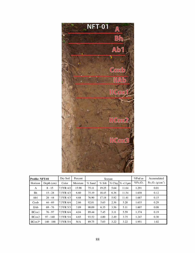
88

89
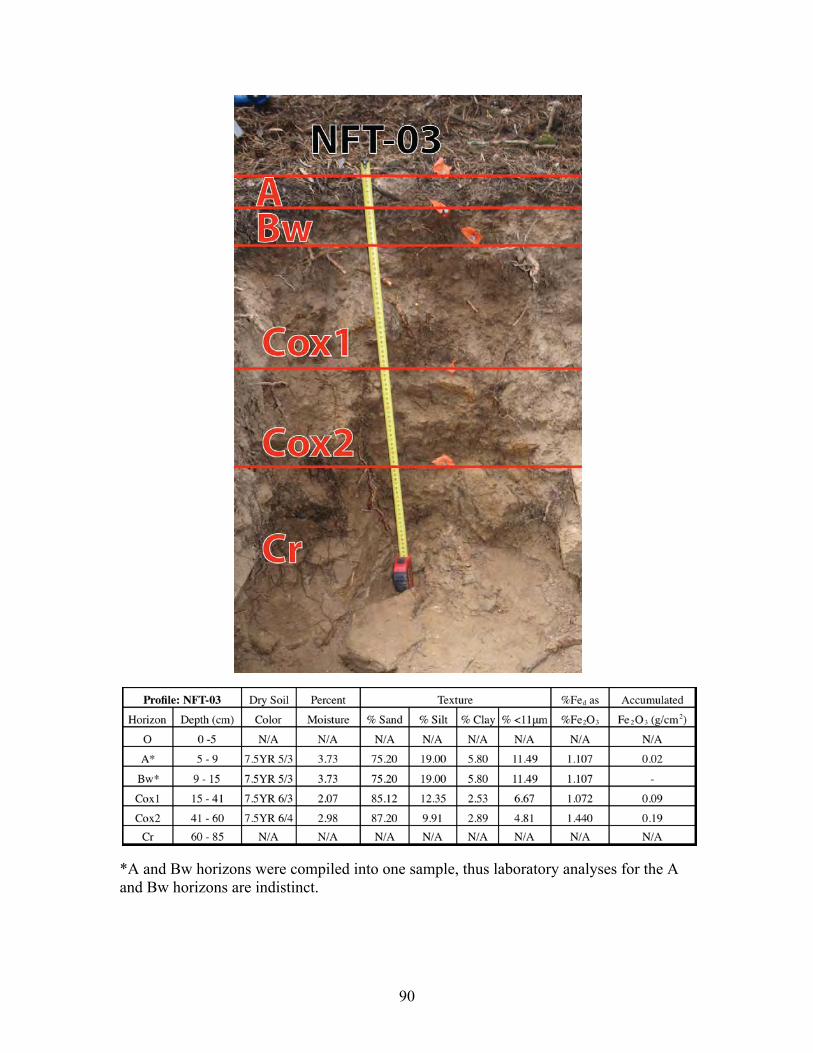
90
*A and Bw horizons were compiled into one sample, thus laboratory analyses for the A and Bw horizons are indistinct.

91
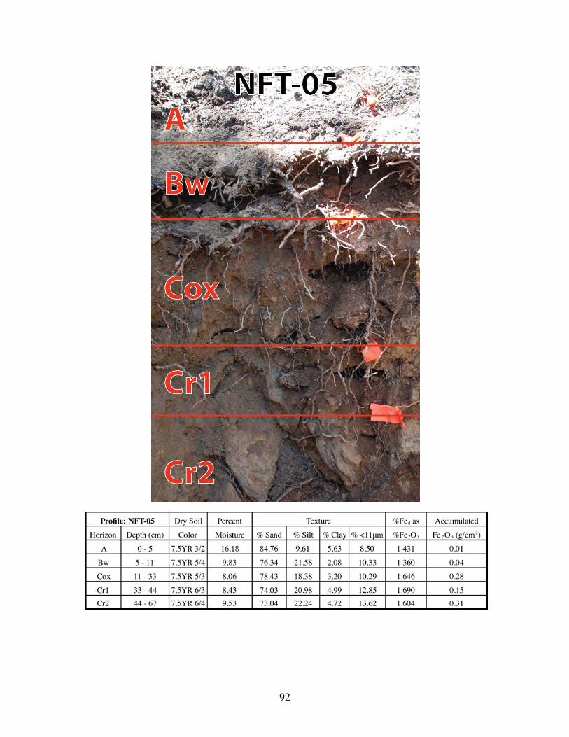
92

93

94

95

96

97

98

99

100
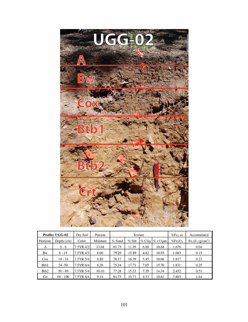
101

102
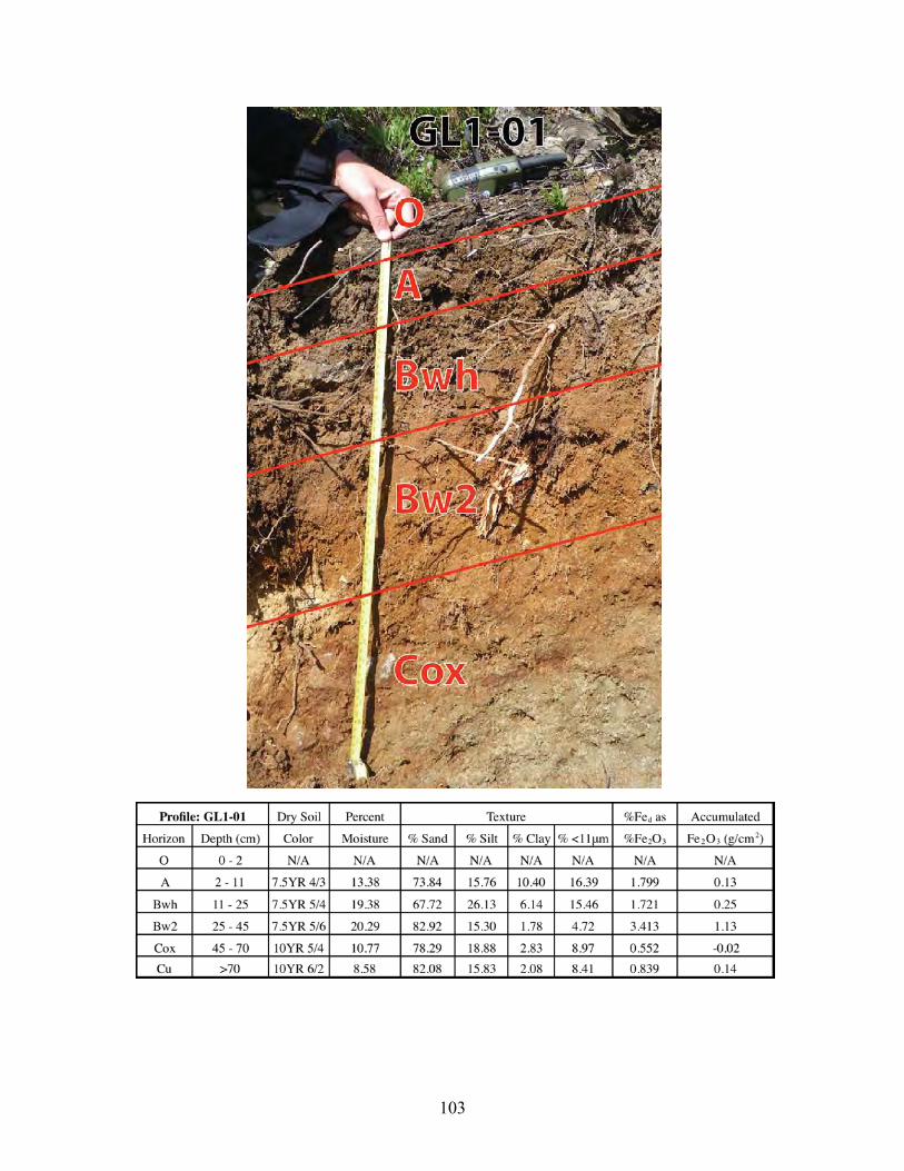
103
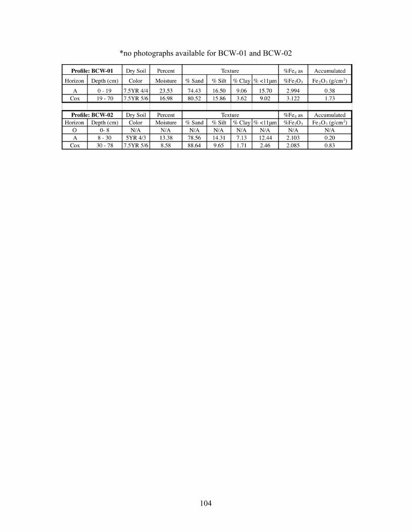
104
*no photographs available for BCW-01 and BCW-02

105
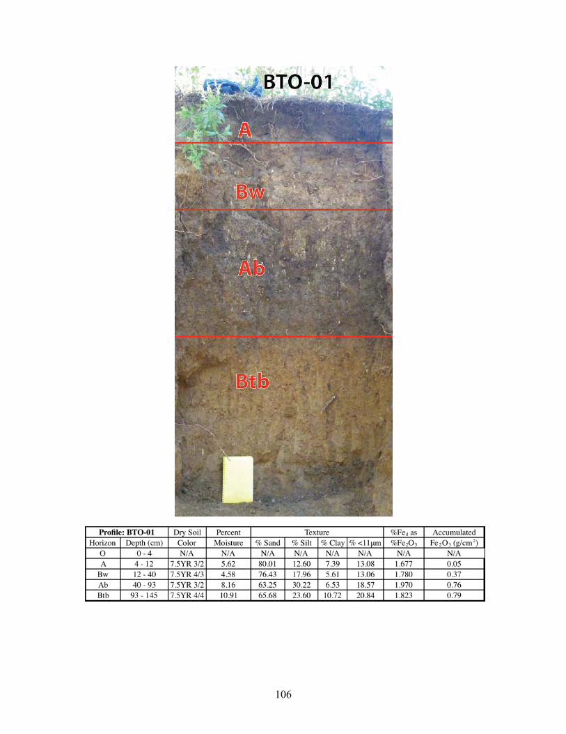
106
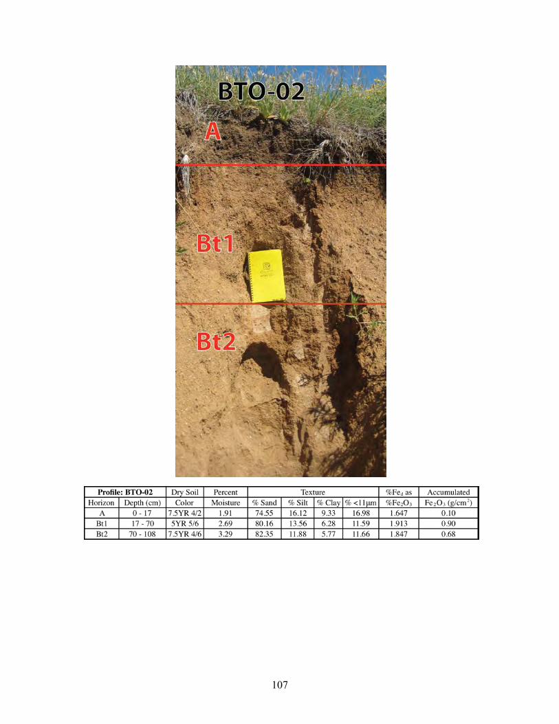
107
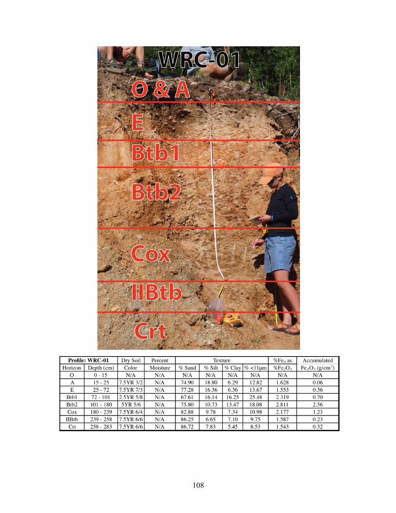
108

No. Sample Name Horizon Top Depth (cm) Bottom Depth (cm) Mean Depth (cm) Thickness (cm) Color Moisture %1 LGG_NFT-05A A 0 5 2.5 5 7.5YR 3/2 16.182 LGG_NFT-05Bw Bw 5 11 8 6 7.5YR 5/4 9.833 LGG_NFT-05Cox Cox1 11 33 22 22 7.5YR 5/3 8.064 LGG_NFT-05Cr1 Cr1 33 44 38.5 11 7.5YR 6/3 8.435 LGG_NFT-05Cr2 Cr2 44 67 55.5 23 7.5YR 6/4 9.536 LGG_NFT-04A/Ej/Bw A/Ej/Bw 5 15 10 10 7.5YR 6/2 6.887 LGG_NFT-04Cox1 Cox1 15 30 22.5 15 7.5YR 6/4 13.668 LGG_NFT-04Cox2 Cox2 30 42 36 12 10YR 5/3 10.549 LGG_NFT-03ABw A/Bw 5 15 10 10 7.5YR 5/3 3.73
10 LGG_NFT-03Cox1 Cox1 15 41 28 26 7.5YR 6/3 2.0711 LGG_NFT-03Cr1 Cox2 41 60 50.5 19 7.5YR 6/4 2.9812 LGG_NFT-02C1 Cox1 5 25 15 20 7.5YR 6/4 2.8713 LGG_NFT-02C2 Cox2 25 65 45 40 7.5YR 6/4 3.5114 LGG_NFT-02C3 Cox3 65 95 80 30 7.5YR 5/4 6.3415 LGG_NFT-02C4 IICox1 95 125 110 30 7.5YR 5/4 5.6416 LGG_NFT-02C5 IICox2 125 175 150 50 7.5YR 5/4 4.4817 LGG_NFT-01A A 8 15 11.5 7 7.5YR 4/2 15.9818 LGG_NFT-01Bh Bh 15 28 21.5 13 7.5YR 4/3 6.6019 LGG_NFT-01Ab1 Ab1 28 44 36 16 7.5YR 4/3 4.6820 LGG_NFT-01Coxb Coxb 44 69 56.5 25 7.5YR 6/4 2.6621 LGG_NFT-01Ab2 IIAb 69 76 72.5 7 7.5YR 5/3 3.8922 LGG_NFT-01Cox1 IICox1 76 97 86.5 21 7.5YR 6/4 4.0423 LGG_NFT-01Cox2 IICox2 97 140 118.5 43 7.5YR 5/4 4.6524 LGG_NFT-01CC143 IICox3 140 153 146.5 13 7.5YR 5/425 LGG_NFT-01CC163 IICox3 153 173 163 20 7.5YR 5/426 LGG_NFT-01CC183 IICox3 173 193 183 20 7.5YR 5/427 LGG_SFT-00A A 0 7 3.5 7 7.5YR 4/2 17.3628 LGG_SFT-00Cox Cox1 7 23 15 16 7.5YR 5/3 11.9829 LGG_SFT-00Cr1 Cox2 23 53 38 30 7.5YR 5/3 3.2530 LGG_SFT-00Cr2 Cr2 53 82 67.5 29 7.5YR 5/4 3.0531 LGG_SFT-01A A 0 28 14 28 7.5YR 4/2 5.7932 LGG_SFT-01Ab Ab 28 42 35 14 7.5YR 4/2 3.7533 LGG_SFT-01Cox Cox 42 50 46 8 10YR 4/3 3.96
109 Appendix B: Complete table of field and laboratory data
109

34 LGG_SFT-01Cr Cr 50 70 60 20 10YR 5/4 5.2135 LGG_SFT-1B_A A 0 10 5 10 10YR 4/2 11.6336 LGG_SFT-1B_Bw Cox1 10 18 14 8 7.5YR 5/4 5.5537 LGG_SFT-1B_Cox Cox2 18 38 28 20 7.5YR 5/4 3.8538 LGG_SFT-1B_Cr Cr 38 68 53 30 7.5YR 5/4 4.0439 LGG_SFT-02A A 2 12 7 10 7.5YR 4/2 10.4040 LGG_SFT-02Cox1 Cox1 12 22 17 10 7.5YR 5/3 7.0241 LGG_SFT-02Cox2 Cox2 22 32 27 10 7.5YR 6/4 3.4142 LGG_SFT-03A A 0 5 2.5 5 7.5YR 4/2 9.1343 LGG_SFT-03Cox1 Cox1 5 20 12.5 15 7.5YR 5/3 7.7444 LGG_SFT-03Cox2 Cox2 20 40 30 20 7.5YR 6/4 6.4545 LGG_SFT-03Cr1 Cr 40 55 47.5 15 7.5YR 7/4 2.2246 GL1-01A A 2 11 6.5 9 7.5YR 4/3 13.3847 GL1-01Bwh Bwh 11 25 18 14 7.5YR 5/4 19.3848 GL1-01Bw2 Bw2 25 45 35 20 7.5YR 5/6 20.2949 GL1-01Cox Cox 45 70 57.5 25 10YR 5/4 10.7750 GL1-01Cu Cu 70 100 85 30 10YR 6/2 8.5851 BCW-01A A 0 19 9.5 19 7.5YR 4/4 23.5352 BCW-01C Bw 19 70 44.5 51 7.5YR 5/6 16.9853 BCW-02A A 8 30 19 22 5YR 4/3 17.9754 BCW-02Bw Bw 30 78 54 48 7.5YR 5/6 4.4155 BCW-03A A 0 9 4.5 9 7.5YR 4/3 18.8656 BCW-03Bw Bw 9 52 30.5 43 7.5YR 4/6 7.5857 BCW-03Cox1 Cox1 52 78 65 26 7.5YR 5/6 8.0958 BCW-03Cox2 Cox2 78 120 99 42 7.5YR 6/6 9.7859 BCW-03Btb Btb 120 160 140 40 7.5YR 5/6 9.8760 BCW_SLQ-01A A 0 9 4.5 9 7.5YR 4/261 BCW_SLQ-01Ej Ej 9 15 12 6 10YR 6/262 BCW_SLQ-01Bw1 Bw1 15 32 23.5 17 10YR 5/463 BCW_SLQ-01Bw2 Bw2 32 48 40 16 10YR 5/464 BCW_SLQ-01Bw3 Bw3 48 66 57 18 10YR 6/465 BCW_SLQ-01Cox Cox 66 102 84 36 2.5Y 5/366 BCW_SLQ-01Cu Cu 102 112 107 10 2.5Y 6/167 BCW_SLQ-01CC205 Cu 20568 BCW_SLQ-01CC305 Cu 305
110 Appendix B: Complete table of field and laboratory data
110

69 BTO-01A A 4 12 8 8 7.5YR 3/2 5.6270 BTO-01Bw Bw 12 40 26 28 7.5YR 4/3 4.5871 BTO-01Ab Ab 40 94 67 54 7.5YR 3/2 8.1672 BTO-01Btb Btb 94 145 119.5 51 7.5YR 4/4 10.9173 BTO-02A A 0 17 8.5 17 7.5YR 4/2 1.9174 BTO-02Bt1 Bt1 17 70 43.5 53 5YR 5/6 2.6975 BTO-02Bt2 Bt2 70 108 89 38 7.5YR 4/6 3.2976 UGG-01Ah Ah 3 7 5 4 7.5YR 5/2 10.6377 UGG-01Bt Btb 42 50 46 8 7.5YR 7/4 9.0678 UGG-01Cox Coxb 76 80 78 4 7.5YR 7/4 8.4579 MGG-01A A 10 23 16.5 13 7.5YR 4/2 11.2580 MGG-01Cox Cox 23 47 35 24 7.5YR 5/3 9.0481 MGG-01Cr1 Cr1 47 60 53.5 13 7.5YR 6/3 6.8882 MGG-01Cr2 Cr2 60 100 80 40 7.5YR 7/3 6.8583 MGG-02A A 0 12 6 12 7.5YR 4/2 18.1684 MGG-02Cox Cox 12 25 18.5 13 7.5YR 6/3 8.6785 MGG-02Cr-I Cr 25 70 47.5 45 7.5YR 7/4 7.6486 MGG-02Cr-II Cr 70 110 90 40 7.5YR 7/6 6.3087 UGG-02A A 0 6 3 6 7.5YR 4/2 13.6888 UGG-02Bw Bw 6 19 12.5 13 7.5YR 4/3 8.0089 UGG-02Cox Cox 19 34 26.5 15 7.5YR 5/4 8.8990 UGG-02Btb1 Btb1 34 50 42 16 7.5YR 6/4 8.2891 UGG-02Btb2 Btb2 50 69 59.5 19 7.5YR 5/4 10.1092 UGG-02Crt Crt 69 100 84.5 31 7.5YR 6/4 9.1493 GL5-001 0 0 7.5YR 4/294 WRC-01A A 15 25 20 10 7.5YR 3/295 WRC-01E E 25 72 48.5 47 7.5YR 7/396 WRC-01Btb1 Btb1 72 101 86.5 29 2.5YR 5/897 WRC-01Btb2 Btb2 101 180 140.5 79 5YR 5/698 WRC-01Cox Cox 180 239 209.5 59 7.5YR 6/499 WRC-01IIBtb IIBtb 239 258 248.5 19 7.5YR 6/6
100 WRC-01Crt Crt 258 283 270.5 25 7.5YR 6/6101 WRC-02A 20 20 7.5YR 6/3102 WRC-02E 110 20 7.5YR 6/4103 WRC-02G 170 20 5YR 6/6
111 Appendix B: Complete table of field and laboratory data
111

104 GRL-3283 A1 0 3 1.5 3105 GRL-3284-1 A2 3 40 21.5 37106 GRL-3284-2 A2 3 40 21.5 37107 GRL-3285 B21t 40 85 62.5 45108 GRL-3286-1 B22t 85 135 110 50109 GRL-3286-2 B22t 85 135 110 50110 GRL-3287 B3 135 155 145 20111 GRL-3288-1 C1ox 155 195 175 40112 GRL-3288-2 C1ox 155 195 175 40113 GRL-3289 C2ox 195 210 202.5 15
112 Appendix B: Complete table of field and laboratory data
112
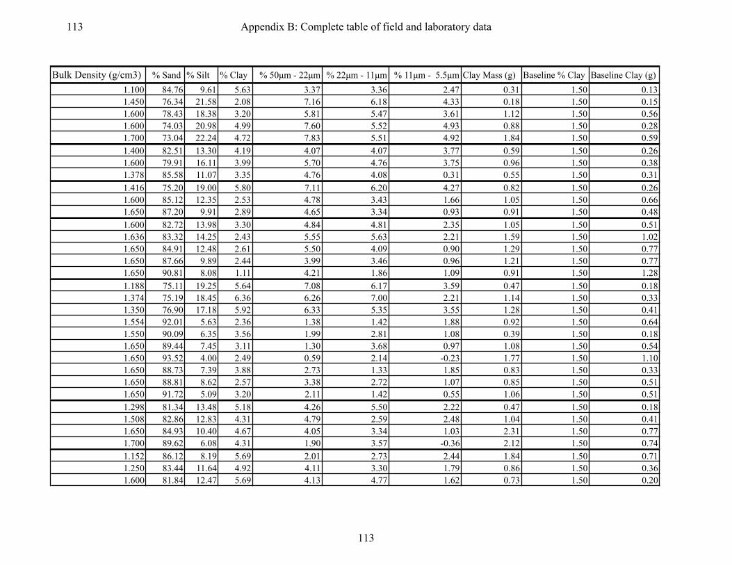
Bulk Density (g/cm3) % Sand % Silt % Clay % 50µm - 22µm % 22µm - 11µm % 11µm - 5.5µm Clay Mass (g) Baseline % Clay Baseline Clay (g)1.100 84.76 9.61 5.63 3.37 3.36 2.47 0.31 1.50 0.131.450 76.34 21.58 2.08 7.16 6.18 4.33 0.18 1.50 0.151.600 78.43 18.38 3.20 5.81 5.47 3.61 1.12 1.50 0.561.600 74.03 20.98 4.99 7.60 5.52 4.93 0.88 1.50 0.281.700 73.04 22.24 4.72 7.83 5.51 4.92 1.84 1.50 0.591.400 82.51 13.30 4.19 4.07 4.07 3.77 0.59 1.50 0.261.600 79.91 16.11 3.99 5.70 4.76 3.75 0.96 1.50 0.381.378 85.58 11.07 3.35 4.76 4.08 0.31 0.55 1.50 0.311.416 75.20 19.00 5.80 7.11 6.20 4.27 0.82 1.50 0.261.600 85.12 12.35 2.53 4.78 3.43 1.66 1.05 1.50 0.661.650 87.20 9.91 2.89 4.65 3.34 0.93 0.91 1.50 0.481.600 82.72 13.98 3.30 4.84 4.81 2.35 1.05 1.50 0.511.636 83.32 14.25 2.43 5.55 5.63 2.21 1.59 1.50 1.021.650 84.91 12.48 2.61 5.50 4.09 0.90 1.29 1.50 0.771.650 87.66 9.89 2.44 3.99 3.46 0.96 1.21 1.50 0.771.650 90.81 8.08 1.11 4.21 1.86 1.09 0.91 1.50 1.281.188 75.11 19.25 5.64 7.08 6.17 3.59 0.47 1.50 0.181.374 75.19 18.45 6.36 6.26 7.00 2.21 1.14 1.50 0.331.350 76.90 17.18 5.92 6.33 5.35 3.55 1.28 1.50 0.411.554 92.01 5.63 2.36 1.38 1.42 1.88 0.92 1.50 0.641.550 90.09 6.35 3.56 1.99 2.81 1.08 0.39 1.50 0.181.650 89.44 7.45 3.11 1.30 3.68 0.97 1.08 1.50 0.541.650 93.52 4.00 2.49 0.59 2.14 -0.23 1.77 1.50 1.101.650 88.73 7.39 3.88 2.73 1.33 1.85 0.83 1.50 0.331.650 88.81 8.62 2.57 3.38 2.72 1.07 0.85 1.50 0.511.650 91.72 5.09 3.20 2.11 1.42 0.55 1.06 1.50 0.511.298 81.34 13.48 5.18 4.26 5.50 2.22 0.47 1.50 0.181.508 82.86 12.83 4.31 4.79 2.59 2.48 1.04 1.50 0.411.650 84.93 10.40 4.67 4.05 3.34 1.03 2.31 1.50 0.771.700 89.62 6.08 4.31 1.90 3.57 -0.36 2.12 1.50 0.741.152 86.12 8.19 5.69 2.01 2.73 2.44 1.84 1.50 0.711.250 83.44 11.64 4.92 4.11 3.30 1.79 0.86 1.50 0.361.600 81.84 12.47 5.69 4.13 4.77 1.62 0.73 1.50 0.20
113 Appendix B: Complete table of field and laboratory data
113

1.700 79.88 14.57 5.55 5.71 2.59 3.80 1.89 1.50 0.511.200 82.00 12.46 5.54 4.96 2.58 2.44 0.66 1.50 0.261.405 82.73 13.06 4.21 4.18 3.36 3.06 0.47 1.50 0.201.600 83.77 12.22 4.01 4.08 2.64 2.54 1.28 1.50 0.511.700 86.92 11.13 1.95 4.07 2.72 2.40 0.99 1.50 0.771.200 84.26 10.67 5.08 2.66 3.36 3.80 0.61 1.50 0.261.600 82.85 13.55 3.60 4.08 4.82 1.67 0.58 1.50 0.261.650 82.12 14.81 3.07 4.79 5.56 1.51 0.51 1.50 0.261.200 88.98 7.93 3.09 1.89 2.85 1.72 0.19 1.50 0.131.600 88.08 9.29 2.63 2.75 3.55 0.98 0.63 1.50 0.381.600 86.82 10.55 2.63 3.42 2.63 2.53 0.84 1.50 0.511.650 82.05 14.71 3.24 6.31 3.14 1.79 0.80 1.50 0.381.500 73.84 15.76 10.40 5.55 4.22 3.06 1.40 2.00 0.361.750 67.72 26.13 6.14 8.99 7.83 4.88 1.51 2.00 0.562.000 82.92 15.30 1.78 7.70 4.66 1.49 0.71 2.00 0.802.000 78.29 18.88 2.83 8.03 4.71 3.74 1.42 2.00 1.002.000 82.08 15.83 2.08 5.53 3.98 4.52 1.25 2.00 1.201.200 74.43 16.50 9.06 5.71 4.16 3.70 2.07 2.00 0.761.600 80.52 15.86 3.62 6.49 3.98 2.43 2.95 2.00 2.041.200 78.56 14.31 7.13 4.97 4.03 2.34 1.88 2.00 0.881.600 88.64 9.65 1.71 4.82 4.08 0.82 1.31 2.00 1.921.200 68.29 22.74 8.97 6.19 6.95 5.12 0.97 2.00 0.361.600 84.05 13.97 1.98 5.57 4.02 2.42 1.36 2.00 1.721.700 81.36 16.67 1.97 7.06 5.38 2.27 0.87 2.00 1.041.700 72.39 25.66 1.94 9.26 8.43 6.20 1.39 2.00 1.681.700 75.90 20.33 3.76 7.16 5.41 4.31 2.56 2.00 1.601.500 75.81 18.19 6.00 7.19 4.71 4.32 0.81 2.00 0.361.700 75.86 21.56 2.57 8.02 8.29 1.34 0.26 2.00 0.242.000 74.86 20.54 4.60 7.95 6.17 2.92 1.57 2.00 0.682.000 80.08 15.76 4.16 7.06 4.66 1.62 1.33 2.00 0.642.000 80.57 17.12 2.30 7.08 7.11 1.97 0.83 2.00 0.722.000 80.68 17.41 1.91 8.43 5.45 2.18 1.37 2.00 1.442.000 68.79 21.63 9.58 6.64 5.51 5.04 1.92 2.00 0.402.000 71.45 21.35 7.19 7.32 4.17 4.42 0.00 0.002.000 71.45 21.35 7.19 7.32 4.17 4.42 0.00 0.00
114 Appendix B: Complete table of field and laboratory data
114

1.200 80.01 12.60 7.39 4.28 2.63 3.74 0.71 2.00 0.271.500 76.43 17.96 5.61 5.78 4.73 2.97 2.36 2.00 0.951.400 63.25 30.22 6.53 8.33 9.85 8.47 4.94 2.00 1.841.600 65.68 23.60 10.72 6.62 6.87 4.65 8.75 2.00 1.731.200 74.55 16.12 9.33 5.70 2.77 3.77 1.90 2.00 0.581.600 80.16 13.56 6.28 4.96 3.29 2.37 5.33 2.00 1.801.700 82.35 11.88 5.77 4.82 1.17 2.48 3.73 2.00 1.291.200 81.57 12.83 5.61 4.13 4.77 3.03 0.27 0.001.600 76.02 14.75 9.23 4.16 4.14 3.04 1.18 0.001.600 66.82 22.60 10.58 5.47 7.03 4.57 0.68 0.001.200 79.21 15.26 5.53 5.04 4.77 2.97 0.86 2.00 0.441.600 79.31 16.15 4.53 4.99 4.75 2.97 1.74 2.00 0.821.700 85.45 10.82 3.73 2.71 2.69 2.44 0.83 2.00 0.441.750 87.67 7.70 4.62 1.91 2.72 1.17 3.24 2.00 1.361.200 77.15 16.52 6.33 5.86 4.73 2.97 0.91 2.00 0.411.600 80.08 14.92 5.00 4.98 4.72 2.27 1.04 2.00 0.441.700 88.05 8.55 3.40 2.73 2.06 1.79 2.60 2.00 1.531.750 86.81 8.51 4.68 1.99 3.48 1.12 3.28 2.00 1.361.200 81.73 11.39 6.88 4.16 3.26 1.05 0.50 2.00 0.201.500 79.29 15.89 4.82 5.04 4.73 1.63 0.94 2.00 0.441.600 78.17 16.39 5.45 5.68 5.49 2.24 1.31 2.00 0.511.600 75.24 17.71 7.05 4.80 4.26 3.69 1.81 2.00 0.541.650 77.28 15.33 7.39 4.24 4.14 3.04 2.32 2.00 0.651.750 84.75 10.73 4.53 3.43 1.22 2.55 2.46 2.00 1.05
74.61 18.61 6.78 5.67 5.52 4.941.200 74.90 18.80 6.29 6.01 6.27 3.56 0.76 2.00 0.351.400 77.28 16.36 6.36 4.18 4.87 4.34 4.18 2.00 1.651.650 67.61 16.14 16.25 4.78 2.14 3.70 7.77 2.00 1.021.650 75.80 10.73 13.47 3.09 3.03 1.97 17.56 2.00 2.771.600 82.88 9.78 7.34 2.80 3.35 1.73 6.93 2.00 2.071.650 86.25 6.65 7.10 2.00 2.00 1.14 2.23 2.00 0.671.750 86.72 7.83 5.45 2.01 2.73 1.17 2.38 2.00 0.88
2.57 3.171.30 1.850.59 1.88
115 Appendix B: Complete table of field and laboratory data
115

1.400 86.20 9.90 3.90 0.16 2.00 0.121.500 74.70 20.00 5.30 2.94 2.00 1.481.500 74.70 20.00 5.30 2.94 2.00 1.482.200 74.20 12.10 13.70 13.56 2.00 1.802.000 67.30 16.90 15.80 15.80 2.00 2.002.000 67.30 16.90 15.80 15.80 2.00 2.002.000 73.30 16.30 10.40 4.16 2.00 0.802.000 66.20 24.90 8.90 7.12 2.00 1.602.000 66.20 24.90 8.90 7.12 2.00 1.602.000 63.40 28.00 8.60 2.58 2.00 0.60
116 Appendix B: Complete table of field and laboratory data
116

Accumulated clay (g) %Fed %Fe2O3 Baseline %Fe2O3 Baseline Fe2O3 (g) Accumulated Fe2O3(g) pH0.18 1.001 1.431 0.800 0.068 0.011 5.230.03 0.951 1.360 0.800 0.082 0.037 5.490.56 1.151 1.646 0.800 0.299 0.280 5.610.60 1.182 1.690 0.800 0.150 0.148 5.71.26 1.122 1.604 0.800 0.313 0.3140.33 0.764 1.092 0.800 0.136 0.017 5.020.57 1.653 2.363 0.800 0.204 0.363 5.010.25 0.811 1.159 0.800 0.163 0.029 5.390.57 0.774 1.107 0.800 0.136 0.021 5.060.39 0.750 1.072 0.800 0.354 0.092 5.050.42 1.007 1.440 0.800 0.258 0.1930.54 1.022 1.461 0.800 0.272 0.196 5.20.57 1.364 1.950 0.800 0.544 0.732 5.390.53 1.502 2.147 0.800 0.408 0.655 5.830.44 1.648 2.356 0.800 0.408 0.758 5.96
-0.36 1.944 2.779 0.800 0.680 1.6130.29 0.903 1.291 0.800 0.095 0.012 5.510.80 1.160 1.658 0.800 0.177 0.119 5.440.87 1.180 1.687 0.800 0.218 0.1470.28 1.142 1.633 0.800 0.340 0.294 5.770.21 1.124 1.607 0.800 0.095 0.0790.54 0.961 1.374 0.800 0.286 0.190 5.830.67 0.872 1.247 0.800 0.585 0.3000.50 1.169 1.671 0.800 0.177 0.1820.34 1.362 1.947 0.800 0.272 0.3710.55 1.562 2.233 0.800 0.272 0.4650.29 1.090 1.558 0.800 0.095 0.046 5.260.63 1.364 1.950 0.800 0.218 0.253 5.771.55 1.386 1.982 0.800 0.408 0.573 5.881.38 1.691 2.418 0.800 0.394 0.7971.12 1.154 1.650 0.800 0.381 0.151 5.660.50 1.285 1.837 0.800 0.190 0.131 5.920.52 1.209 1.729 0.800 0.109 0.112 5.85
117 Appendix B: Complete table of field and laboratory data
117

1.38 1.347 1.926 0.800 0.272 0.383 5.940.41 1.124 1.607 0.800 0.136 0.057 5.460.27 1.314 1.879 0.800 0.109 0.102 5.870.77 1.314 1.879 0.800 0.272 0.329 5.970.23 1.187 1.697 0.800 0.408 0.4570.35 0.945 1.351 0.800 0.136 0.026 5.190.32 0.990 1.415 0.800 0.136 0.090 5.590.25 1.051 1.503 0.800 0.136 0.1120.06 0.863 1.234 0.800 0.068 0.006 5.180.25 0.626 0.895 0.800 0.204 0.011 5.690.33 0.752 1.075 0.800 0.272 0.072 5.680.42 0.857 1.225 0.800 0.204 0.099 5.721.04 1.258 1.799 0.600 0.108 0.135 5.060.95 1.204 1.721 0.600 0.168 0.254 5.05
-0.09 2.387 3.413 0.600 0.240 1.125 4.790.42 0.386 0.552 0.600 0.300 -0.024 5.650.05 0.587 0.839 0.600 0.360 0.144 5.511.31 2.094 2.994 0.800 0.304 0.3790.91 2.184 3.122 0.800 0.816 1.7321.00 1.471 2.103 0.800 0.352 0.203
-0.61 1.458 2.085 0.800 0.768 0.833 4.860.61 1.213 1.734 0.800 0.144 0.043 4.48
-0.36 1.597 2.283 0.800 0.688 0.883 4.83-0.17 1.189 1.700 0.800 0.416 0.335 5.04-0.29 1.047 1.497 0.800 0.672 0.397 5.080.96 1.434 2.050 0.800 0.640 0.754 5.10.45 0.467 0.668 0.600 0.108 -0.0180.02 0.385 0.550 0.600 0.072 -0.016 4.510.89 1.937 2.769 0.600 0.204 0.738 4.40.69 1.442 2.062 0.600 0.192 0.468 4.860.11 0.746 1.067 0.600 0.216 0.168 4.89
-0.07 0.491 0.702 0.600 0.432 0.073 5.051.52 0.437 0.625 0.600 0.120 0.005 5.840.00 0.418 0.598 0.000 0.0000.00 0.439 0.628 0.000 0.000
118 Appendix B: Complete table of field and laboratory data
118

0.44 1.173 1.677 0.800 0.109 0.052 5.571.41 1.245 1.780 0.800 0.381 0.367 5.853.10 1.378 1.970 0.800 0.734 0.755 6.187.02 1.275 1.823 0.800 0.694 0.794 6.051.32 1.152 1.647 0.800 0.231 0.1053.53 1.338 1.913 0.800 0.721 0.9012.43 1.292 1.847 0.800 0.517 0.6760.27 0.926 1.324 0.800 0.054 0.009 5.351.18 1.174 1.678 0.800 0.109 0.106 5.750.68 1.768 2.528 0.800 0.054 0.1070.42 1.250 1.787 0.800 0.177 0.1020.92 1.185 1.694 0.800 0.326 0.3240.38 2.063 2.949 0.800 0.177 0.4751.88 1.151 1.646 0.800 0.544 0.6080.50 1.191 1.703 0.800 0.163 0.0820.60 1.306 1.867 0.800 0.177 0.2121.07 1.129 1.614 0.800 0.612 0.6231.92 2.044 2.922 0.800 0.544 1.5020.29 1.172 1.676 0.800 0.082 0.039 5.610.50 1.177 1.683 0.800 0.177 0.151 5.390.80 1.271 1.817 0.800 0.204 0.232 5.41.26 1.281 1.831 0.800 0.218 0.251 5.891.67 1.715 2.452 0.800 0.258 0.510 5.961.40 2.660 3.803 0.800 0.422 1.642 5.87
0.464 0.6630.41 1.139 1.628 0.800 0.140 0.055 5.682.54 1.086 1.553 0.800 0.658 0.364 5.616.76 1.622 2.319 0.800 0.406 0.704 5.14
14.79 1.966 2.811 0.800 1.106 2.558 5.314.87 1.523 2.177 0.800 0.826 1.229 5.821.56 1.110 1.587 0.800 0.266 0.232 5.761.51 1.079 1.543 0.800 0.350 0.325 5.540.00 0.983 1.4050.00 1.200 1.7160.00 1.445 2.066
119 Appendix B: Complete table of field and laboratory data
119

0.04 0.817 1.168 0.600 0.032 0.0181.46 0.903 1.291 0.600 0.389 0.3281.46 0.883 1.262 0.600 0.389 0.312
11.76 1.512 2.162 0.600 0.473 1.66813.80 1.747 2.498 0.600 0.525 1.97313.80 1.776 2.539 0.600 0.525 2.014
3.36 1.629 2.329 0.600 0.210 0.7225.52 1.055 1.508 0.600 0.420 0.7875.52 1.104 1.578 0.600 0.420 0.8431.98 0.855 1.222 0.600 0.158 0.209
120 Appendix B: Complete table of field and laboratory data
120

121
APPENDIX C: Bulk Geochemical Analysis Sample key for bulk geochemistry analysis. SAMPLE NAME <150 μm >150 μm SAMPLE NAME <150 μm >150 μm UGG-‐02Cox 01-‐A 01-‐B MGG-‐02A 51-‐A 51-‐B UGG-‐02A 02-‐A 02-‐B MGG-‐02Cox 52-‐A 52-‐B UGG-‐02Bw 03-‐A 03-‐B MGG-‐02Cr-‐I 53-‐A 53-‐B UGG-‐02Btb1 04-‐A 04-‐B MGG-‐02Cr-‐II 54-‐A 54-‐B UGG-‐02Btb2 05-‐A 05-‐B LGG_SFT-‐01A 55-‐A 55-‐B UGG-‐02Crt 06-‐A 05-‐B LGG_SFT-‐01Ab 56-‐A 56-‐B BTO-‐01A 07-‐A 07-‐B LGG_SFT-‐01Cox 57-‐A 57-‐B BTO-‐01Bw 08-‐A 08-‐B LGG_SFT-‐01Cr 58-‐A 58-‐B BTO-‐01Ab 09-‐A 09-‐B LGG_SFT-‐00A 59-‐A 59-‐B BTO-‐01Btb 10-‐A 10-‐B LGG_SFT-‐00Cox 60-‐A 60-‐B WRC-‐01A 11-‐A 11-‐B LGG_SFT-‐00Cr1 61-‐A 61-‐B WRC-‐01E 12-‐A 12-‐B LGG_SFT-‐00Cr2 62-‐A 62-‐B WRC-‐01Btb1 13-‐A 13-‐B LGG_NFT-‐05A 63-‐A 63-‐B WRC-‐01Btb2 14-‐A 14-‐B LGG_NFT-‐05Bw 64-‐A 64-‐B WRC-‐01Cox 15-‐A 15-‐B LGG_NFT-‐05Cox 65-‐A 65-‐B WRC-‐01IIBtb 16-‐A 16-‐B LGG_NFT-‐05Cr1 66-‐A 66-‐B WRC-‐01Crt 17-‐A 17-‐B LGG_NFT-‐05Cr2 67-‐A 67-‐B BCW-‐SLQ-‐01A 18-‐A 18-‐B LGG_NFT-‐03ABw 68-‐A 68-‐B BCW-‐SLQ-‐01Ej 19-‐A 19-‐B LGG_NFT-‐03Cox 69-‐A 69-‐B BCW-‐SLQ-‐01Bw1 20-‐A 20-‐B LGG_NFT-‐03Cr1 70-‐A 70-‐B BCW-‐SLQ-‐01Bw2 21-‐A 21-‐B MGG-‐01A 71-‐A 71-‐B BCW-‐SLQ-‐01Bw3 22-‐A 22-‐B MGG-‐01Cox 72-‐A 72-‐B BCW-‐SLQ-‐01Cox 23-‐A 23-‐B MGG-‐01Cr1 73-‐A 73-‐B BCW-‐SLQ-‐01Cu 24-‐A 24-‐B MGG-‐01Cr2 74-‐A 74-‐B UGG-‐01Ah 25-‐A 25-‐B LGG_NFT-‐04A/Ej/Bw 75-‐A 75-‐B UGG-‐01Bt 26-‐A 26-‐B LGG_NFT-‐04Cox 76-‐A 76-‐B UGG-‐01Cox 27-‐A 27-‐B LGG_NFT-‐04Cr1 77-‐A 77-‐B BTO-‐02A 28-‐A 28-‐B BCW-‐02A 78-‐A 78-‐B BTO-‐02Bt1 29-‐A 29-‐B BCW-‐02Bw 79-‐A 79-‐B BTO-‐02Bt2 30-‐A 30-‐B LGG_NFT-‐02C1 80-‐A 80-‐B LGG_SFT-‐03A 31-‐A 31-‐B LGG_NFT-‐02C2 81-‐A 81-‐B LGG_SFT-‐03Cox1 32-‐A 32-‐B LGG_NFT-‐02C3 82-‐A 81-‐B LGG_SFT-‐03Cox2 33-‐A 33-‐B LGG_NFT-‐02C4 83-‐A 83-‐B LGG_SFT-‐03Cr 34-‐A 34-‐B LGG_NFT-‐02C5 84-‐A 84-‐B LGG_SFT-‐1B_A 35-‐A 35-‐B BCW-‐03A 85-‐A 85-‐B LGG_SFT-‐1B_Bw 36-‐A 36-‐B BCW-‐03Bw 86-‐A 86-‐B LGG_SFT-‐1B_Cox 37-‐A 37-‐B BCW-‐03Btb 87-‐A 87-‐B LGG_SFT-‐1B_Cr 38-‐A 38-‐B BCW-‐03Cox1 88-‐A 88-‐B GL1-‐01A 39-‐A 39-‐B BCW-‐03Cox2 89-‐A 89-‐B GL1-‐01Bwh 40-‐A 40-‐B LGG_NFT-‐01A 90-‐A 90-‐B GL1-‐01Bw2 41-‐A 41-‐B LGG_NFT-‐01Bh 91-‐A 91-‐B GL1-‐01Cox 42-‐A 42-‐B LGG_NFT-‐01Ab1 92-‐A 92-‐B GL1-‐01Cu 43-‐A 43-‐B LGG_NFT-‐01Coxb 93-‐A 93-‐B LGG_SFT-‐02A 44-‐A 44-‐B LGG_NFT-‐01Ab2 94-‐A 94-‐B LGG_SFT-‐02Cox1 45-‐A 45-‐B LGG_NFT-‐01Cox1 95-‐A 95-‐B LGG_SFT-‐02Cox2 46-‐A 46-‐B LGG_NFT-‐01Cox2 96-‐A 96-‐B WRC-‐02A 47-‐A 47-‐B BCW-‐001A 97-‐A 97-‐B WRC-‐02E 48-‐A 48-‐B BCW-‐001C 98-‐A 98-‐B WRC-‐02G 49-‐A 49-‐B GL5-‐001 50-‐A 50-‐B

1020 Cordova St. East Vancouver BC V6A 4A3 Canada
Client:
Submitted By:
Receiving Lab:
Received:
Report Date:
Page:
Dept. of Geosciences
947 Main Street, Clark Hall
Williamstown MA 01267 USA
David Dethier
Canada-Vancouver
March 10, 2011
Method
Code
Code Description Report
Status
SAMPLE PREPARATION AND ANALYTICAL PROCEDURES
Test
Wgt (g)
Number of
Samples
Lab
Soil Pulverize Soil Pulverize14 VAN
4A4B Whole Rock Analysis Majors and Trace Elements Completed0.226 VAN
ADDITIONAL COMMENTS
CC:
Invoice To:
This report supersedes all previous preliminary and final reports with this file number dated prior to the date on this certificate. Signature indicates final approval; preliminary reports are unsigned and should be used for reference only.All results are considered the confidential property of the client. Acme assumes the liabilities for actual cost of analysis only.“*” asterisk indicates that an analytical result could not be provided due to unusually high levels of interference from other elements.
Acme does not accept responsibility for samples left at the laboratory after 90
days without prior written instructions for sample storage or return.
Store After 90 days Invoice for StorageSTOR-PLP
26
None Given
Number of Samples:
P.O. Number
Shipment ID:
Project:
SAMPLE DISPOSAL
CERTIFICATE OF ANALYSIS VAN11001056.1
CLIENT JOB INFORMATION
Williams College
Dept. of Geosciences
947 Main Street, Clark Hall
Williamstown MA 01267
USA
1 of 2
March 30, 2011www.acmelab.com
Williams College
Acme Analytical Laboratories (Vancouver) Ltd.
122

2 of 2
None Given
Dept. of Geosciences
947 Main Street, Clark Hall
Williamstown MA 01267 USA
Project:
Page:
Report Date:
Phone (604) 253-3158 Fax (604) 253-1716
1020 Cordova St. East Vancouver BC V6A 4A3 Canada
1Part
March 30, 2011
www.acmelab.com
Client: Williams College
Acme Analytical Laboratories (Vancouver) Ltd.
CERTIFICATE OF ANALYSIS VAN11001056.1 CERTIFICATE OF ANALYSIS VAN11001056.1
MDL
Unit
Analyte
Method WGHT 4A-4B 4A-4B 4A-4B 4A-4B 4A-4B 4A-4B 4A-4B 4A-4B 4A-4B 4A-4B 4A-4B 4A-4B 4A-4B 4A-4B 4A-4B 4A-4B 4A-4B 4A-4B 4A-4B
Wgt SiO2 Al2O3 Fe2O3 MgO CaO Na2O K2O TiO2 P2O5 MnO Cr2O3 Ni Sc LOI Sum Ba Be Co Cs
kg % % % % % % % % % % % ppm ppm % % ppm ppm ppm ppm
0 0.01 0.01 0.04 0.01 0.01 0.01 0.01 0.01 0.01 0.01 0.002 20 1 -5.1 0.01 1 1 0.2 0.1
59-C Rock Pulp 54.28 17.98 5.56 1.23 1.01 1.14 2.86 0.82 0.12 0.08 0.013 30 13 14.6 99.68 633 3 14.1 5.3
59-B Soil 65.73 14.94 5.18 0.88 0.73 1.22 3.70 0.62 0.08 0.07 0.031 22 12 6.6 99.78 913 2 10.2 3.2
62-C Rock Pulp 55.05 21.25 7.58 1.28 1.39 1.97 2.55 0.77 0.10 0.07 0.013 41 19 7.7 99.68 574 4 13.7 6.6
62-B Soil 75.42 11.94 4.56 0.67 1.13 1.68 1.61 0.44 0.04 0.06 0.027 24 14 2.3 99.88 450 2 7.9 2.7
35-A Rock Pulp 57.37 16.99 5.79 1.40 1.51 1.71 2.96 0.78 0.16 0.09 0.022 33 13 11.0 99.72 724 3 12.8 3.6
35-B Soil 69.41 14.14 4.11 0.80 1.02 1.66 3.84 0.50 0.09 0.05 0.006 21 9 4.2 99.79 983 2 7.9 2.3
38-C Rock Pulp 54.33 23.97 6.33 1.39 1.24 1.88 2.89 0.98 0.11 0.02 0.012 28 14 6.5 99.66 601 4 11.1 3.9
38-B Soil 71.19 13.78 4.58 0.97 0.94 1.57 3.41 0.58 0.06 0.03 0.027 24 9 2.7 99.80 894 3 9.2 2.2
90-B Soil 67.53 12.15 3.45 0.69 0.84 1.38 3.51 0.49 0.12 0.13 0.005 <20 8 9.5 99.76 898 1 7.0 2.5
80-C Rock Pulp 60.19 19.97 5.27 1.27 0.89 1.67 2.92 1.01 0.08 0.02 0.016 27 12 6.3 99.58 571 4 10.2 4.9
80-B Soil 73.31 12.99 3.52 0.81 0.88 1.64 3.15 0.61 0.05 0.02 0.032 <20 8 2.8 99.82 705 2 7.6 1.9
84-C Rock Pulp 50.89 26.43 7.92 1.28 0.70 1.35 3.57 0.99 0.09 0.04 0.019 39 21 6.3 99.61 553 7 12.3 5.3
84-B Soil 65.95 16.49 6.50 1.09 0.45 1.33 3.89 0.83 0.06 0.06 0.011 27 18 3.1 99.79 743 4 12.1 3.1
68-C Rock Pulp 66.36 15.64 4.20 1.08 0.78 1.53 2.70 0.88 0.09 0.04 0.010 22 10 6.4 99.73 753 2 9.7 5.0
68-B Soil 72.71 12.62 3.27 0.59 0.72 1.58 3.80 0.45 0.07 0.05 0.027 <20 9 3.9 99.81 979 1 6.0 2.0
70-C Rock Pulp 63.36 18.02 5.16 1.04 0.89 1.81 2.98 0.84 0.12 0.02 0.009 31 11 5.4 99.64 616 2 9.6 4.0
70-B Soil 68.40 14.87 4.58 0.95 0.99 2.00 4.36 0.72 0.08 0.02 0.005 22 11 2.8 99.77 973 1 9.3 2.3
02-C Rock Pulp 58.38 15.84 4.68 1.13 1.11 1.20 2.85 0.75 0.13 0.13 0.011 35 13 13.5 99.72 814 2 13.5 4.5
02-B Soil 66.98 13.91 4.76 0.75 0.56 1.28 3.80 0.63 0.09 0.08 0.033 27 10 7.0 99.84 698 <1 10.5 2.4
06-A Rock Pulp 52.13 18.35 9.38 1.96 2.37 0.80 4.06 1.51 1.89 0.05 0.014 72 31 6.8 99.32 560 2 20.6 7.6
06-B Soil 56.92 17.02 9.95 2.06 0.70 0.91 4.20 1.60 0.57 0.05 0.013 66 35 5.5 99.49 430 2 24.3 6.9
39-C Rock Pulp 57.46 13.39 5.06 1.40 1.26 1.38 2.57 0.70 0.16 0.05 0.007 <20 10 16.3 99.77 710 1 7.7 5.3
39-B Soil 66.86 13.06 3.23 0.84 1.06 1.91 4.27 0.41 0.10 0.03 0.032 <20 6 8.0 99.83 796 <1 4.9 2.5
43-C Rock Pulp 55.58 19.04 7.63 2.45 1.50 1.90 4.36 0.83 0.29 0.09 0.011 34 16 6.0 99.68 855 3 16.8 4.8
43-B Soil 69.76 14.41 4.02 1.11 1.53 2.41 4.18 0.47 0.16 0.05 0.006 <20 8 1.7 99.80 816 2 7.7 1.9
18-B Soil 70.27 12.31 5.03 0.49 1.29 1.82 3.25 0.82 0.07 0.04 0.037 <20 7 4.4 99.80 864 1 4.7 2.0
This report supersedes all previous preliminary and final reports with this file number dated prior to the date on this certificate. Signature indicates final approval; preliminary reports are unsigned and should be used for reference only. This report supersedes all previous preliminary and final reports with this file number dated prior to the date on this certificate. Signature indicates final approval; preliminary reports are unsigned and should be used for reference only.123
2 of 2
None Given
Dept. of Geosciences
947 Main Street, Clark Hall
Williamstown MA 01267 USA
Project:
Page:
Report Date:
Phone (604) 253-3158 Fax (604) 253-1716
1020 Cordova St. East Vancouver BC V6A 4A3 Canada
2Part
March 30, 2011
www.acmelab.com
Client: Williams College
Acme Analytical Laboratories (Vancouver) Ltd.
CERTIFICATE OF ANALYSIS VAN11001056.1 CERTIFICATE OF ANALYSIS VAN11001056.1
MDL
Unit
Analyte
Method 4A-4B 4A-4B 4A-4B 4A-4B 4A-4B 4A-4B 4A-4B 4A-4B 4A-4B 4A-4B 4A-4B 4A-4B 4A-4B 4A-4B 4A-4B 4A-4B 4A-4B 4A-4B 4A-4B 4A-4B
Ga Hf Nb Rb Sn Sr Ta Th U V W Zr Y La Ce Pr Nd Sm Eu Gd
ppm ppm ppm ppm ppm ppm ppm ppm ppm ppm ppm ppm ppm ppm ppm ppm ppm ppm ppm ppm
0.5 0.1 0.1 0.1 1 0.5 0.1 0.2 0.1 8 0.5 0.1 0.1 0.1 0.1 0.02 0.3 0.05 0.02 0.05
59-C Rock Pulp 23.9 20.7 19.7 128.9 3 155.2 1.1 52.7 7.5 96 3.3 740.3 50.6 127.2 270.5 30.64 119.6 18.70 1.94 14.52
59-B Soil 18.2 7.3 13.7 126.1 1 203.3 0.7 32.1 3.6 68 1.4 251.9 33.9 71.0 155.8 17.50 66.6 10.87 1.47 8.34
62-C Rock Pulp 24.8 25.2 17.2 126.1 2 194.0 0.9 34.2 7.3 99 1.6 902.7 51.5 99.5 207.3 24.20 95.6 15.71 2.45 12.78
62-B Soil 13.0 6.1 9.9 65.0 <1 165.1 0.6 13.5 2.1 44 <0.5 220.0 32.0 39.0 84.1 9.46 37.1 6.23 1.24 5.16
35-A Rock Pulp 21.3 12.1 17.2 130.3 2 224.8 1.0 48.6 5.6 88 2.8 424.8 43.5 108.1 235.1 26.11 102.2 16.75 1.74 12.51
35-B Soil 16.8 7.2 10.4 120.8 2 252.1 0.6 24.7 2.8 55 1.2 250.0 23.1 52.9 113.5 12.69 49.0 8.30 1.25 6.22
38-C Rock Pulp 33.5 26.2 22.6 149.1 1 160.5 1.1 53.2 7.7 103 0.8 902.2 39.3 134.2 279.4 30.31 115.9 17.83 1.85 13.39
38-B Soil 17.7 7.6 15.2 131.9 <1 177.2 0.8 21.6 2.9 64 <0.5 277.3 16.5 54.5 113.0 12.28 47.2 7.39 1.17 5.49
90-B Soil 14.1 7.9 11.3 108.9 1 187.8 0.6 24.3 2.6 45 2.2 282.4 22.6 50.3 110.7 12.25 48.7 7.56 1.11 5.79
80-C Rock Pulp 26.1 50.5 24.0 162.3 2 176.5 1.2 41.7 7.8 94 1.4 1775 42.9 97.7 210.3 23.31 91.0 14.47 1.32 10.85
80-B Soil 16.0 11.5 15.3 117.5 <1 198.3 0.7 18.9 2.3 49 0.6 410.2 19.4 43.2 92.5 10.37 39.3 6.49 1.11 5.04
84-C Rock Pulp 38.0 34.4 23.3 159.8 5 141.2 1.1 68.1 8.7 123 1.1 1187 71.4 157.0 300.3 35.98 138.5 21.93 2.42 16.78
84-B Soil 20.3 8.5 19.6 141.2 1 138.4 1.1 36.6 3.8 80 0.5 287.6 38.9 74.6 145.9 17.54 65.2 10.59 1.43 8.30
68-C Rock Pulp 18.7 20.1 20.8 121.2 2 166.6 1.3 29.6 5.0 76 1.9 714.1 32.4 70.4 146.6 17.07 65.4 10.57 1.13 8.02
68-B Soil 12.6 6.5 10.7 109.2 1 196.5 0.6 22.6 2.2 39 0.8 230.4 27.6 45.9 96.0 11.12 42.9 6.84 1.10 5.30
70-C Rock Pulp 21.4 32.9 19.4 137.2 2 175.8 1.0 71.8 7.4 84 1.2 1144 43.7 150.6 316.6 36.65 142.6 22.15 1.46 16.08
70-B Soil 16.1 8.5 16.2 148.3 1 231.1 0.7 38.4 2.7 60 <0.5 285.7 22.0 79.8 166.4 19.55 73.1 11.65 1.38 7.97
02-C Rock Pulp 19.9 13.7 16.0 132.3 5 217.0 1.0 31.1 5.9 78 5.2 475.4 46.5 85.2 173.3 20.42 81.4 13.51 2.20 10.67
02-B Soil 16.9 5.8 11.0 139.0 3 165.0 0.7 19.0 3.2 69 1.4 196.5 30.3 44.5 92.6 11.05 42.3 7.62 1.26 6.19
06-A Rock Pulp 25.9 17.3 33.7 218.6 15 495.3 1.6 135.3 28.7 134 7.8 622.1 195.2 369.8 811.6 100.0 398.4 70.45 8.42 56.72
06-B Soil 28.7 14.0 40.4 233.2 17 251.4 2.1 108.8 22.2 131 7.5 491.6 195.7 237.1 520.5 62.83 245.8 46.79 4.39 40.91
39-C Rock Pulp 20.0 11.1 16.9 139.5 3 216.2 1.2 29.8 4.6 86 1.8 378.3 26.8 61.7 134.7 16.11 61.8 9.70 1.18 6.81
39-B Soil 16.1 4.5 11.9 162.3 2 242.2 0.7 21.2 2.6 49 0.9 160.5 15.1 43.5 95.3 11.78 44.9 6.91 0.95 4.29
43-C Rock Pulp 25.5 12.5 22.7 201.8 5 273.8 1.3 57.4 7.0 101 2.1 417.9 38.2 101.4 228.9 27.05 105.4 16.01 1.91 11.20
43-B Soil 16.2 5.0 13.7 151.6 3 330.1 0.8 24.6 3.1 60 1.0 165.7 19.0 51.7 112.3 13.76 54.4 8.42 1.22 5.74
18-B Soil 16.5 8.4 16.7 125.0 3 241.1 1.1 19.3 2.9 77 1.0 304.9 31.1 60.1 132.8 16.40 64.5 10.26 1.66 7.35
This report supersedes all previous preliminary and final reports with this file number dated prior to the date on this certificate. Signature indicates final approval; preliminary reports are unsigned and should be used for reference only. This report supersedes all previous preliminary and final reports with this file number dated prior to the date on this certificate. Signature indicates final approval; preliminary reports are unsigned and should be used for reference only.124

2 of 2
None Given
Dept. of Geosciences
947 Main Street, Clark Hall
Williamstown MA 01267 USA
Project:
Page:
Report Date:
Phone (604) 253-3158 Fax (604) 253-1716
1020 Cordova St. East Vancouver BC V6A 4A3 Canada
3Part
March 30, 2011
www.acmelab.com
Client: Williams College
Acme Analytical Laboratories (Vancouver) Ltd.
CERTIFICATE OF ANALYSIS VAN11001056.1 CERTIFICATE OF ANALYSIS VAN11001056.1
MDL
Unit
Analyte
Method 4A-4B 4A-4B 4A-4B 4A-4B 4A-4B 4A-4B 4A-4B 2A Leco 2A Leco 1DX 1DX 1DX 1DX 1DX 1DX 1DX 1DX 1DX 1DX 1DX
Tb Dy Ho Er Tm Yb Lu TOT/C TOT/S Mo Cu Pb Zn Ni As Cd Sb Bi Ag Au
ppm ppm ppm ppm ppm ppm ppm % % ppm ppm ppm ppm ppm ppm ppm ppm ppm ppm ppb
0.01 0.05 0.02 0.03 0.01 0.05 0.01 0.02 0.02 0.1 0.1 0.1 1 0.1 0.5 0.1 0.1 0.1 0.1 0.5
59-C Rock Pulp 1.97 9.64 1.75 4.90 0.69 4.52 0.72 4.90 <0.02 1.5 91.9 40.3 100 30.0 4.4 0.5 0.2 0.2 0.1 3.0
59-B Soil 1.16 5.94 1.19 3.53 0.51 3.33 0.49 2.26 <0.02 6.6 21.7 21.5 60 22.0 2.3 0.2 <0.1 0.1 <0.1 2.0
62-C Rock Pulp 1.80 9.53 1.86 5.47 0.82 5.56 0.84 0.95 <0.02 1.9 82.4 21.5 87 35.8 3.3 0.1 <0.1 <0.1 0.1 4.8
62-B Soil 0.83 5.17 1.15 3.72 0.61 3.99 0.60 0.13 <0.02 6.5 16.1 8.9 39 20.5 0.9 <0.1 <0.1 <0.1 <0.1 0.6
35-A Rock Pulp 1.73 8.47 1.53 4.33 0.59 3.77 0.57 3.49 0.02 3.6 42.0 30.6 92 29.6 4.7 0.4 0.2 0.2 <0.1 5.8
35-B Soil 0.88 4.32 0.81 2.31 0.34 2.09 0.32 1.07 <0.02 1.2 22.0 13.8 55 18.8 2.2 0.2 0.1 <0.1 <0.1 1.5
38-C Rock Pulp 1.77 8.42 1.36 3.64 0.51 3.27 0.51 0.63 <0.02 1.3 58.3 11.6 93 27.0 2.5 <0.1 <0.1 <0.1 <0.1 2.2
38-B Soil 0.73 3.39 0.59 1.71 0.25 1.61 0.25 0.15 <0.02 5.8 20.1 7.0 61 23.5 1.3 <0.1 <0.1 <0.1 <0.1 <0.5
90-B Soil 0.79 3.99 0.81 2.38 0.36 2.54 0.38 3.11 <0.02 1.2 10.9 23.8 72 13.9 2.5 0.3 0.2 0.2 <0.1 <0.5
80-C Rock Pulp 1.52 7.77 1.54 4.60 0.74 5.16 0.90 0.58 <0.02 1.7 21.7 13.5 71 27.1 1.9 <0.1 <0.1 0.1 <0.1 1.8
80-B Soil 0.69 3.58 0.69 2.10 0.34 2.24 0.37 0.37 <0.02 6.4 8.2 7.4 45 17.2 0.8 <0.1 <0.1 <0.1 <0.1 <0.5
84-C Rock Pulp 2.31 12.32 2.60 8.22 1.27 8.41 1.31 0.28 <0.02 2.7 90.5 27.4 101 33.3 2.0 <0.1 <0.1 <0.1 <0.1 2.1
84-B Soil 1.17 6.49 1.30 4.11 0.69 4.52 0.67 0.13 <0.02 1.9 31.0 16.9 74 25.1 1.4 <0.1 <0.1 <0.1 <0.1 <0.5
68-C Rock Pulp 1.15 5.66 1.12 3.23 0.51 3.41 0.53 1.06 <0.02 0.8 26.2 22.1 94 19.0 3.4 <0.1 0.2 0.2 <0.1 2.8
68-B Soil 0.79 4.32 0.90 2.95 0.44 2.83 0.45 1.02 <0.02 6.1 6.2 14.0 46 12.3 1.9 <0.1 0.1 <0.1 <0.1 <0.5
70-C Rock Pulp 1.99 8.62 1.43 3.90 0.63 3.94 0.63 0.46 <0.02 1.2 27.4 13.4 62 21.4 2.5 <0.1 <0.1 0.1 <0.1 0.7
70-B Soil 1.00 4.34 0.79 2.19 0.32 2.09 0.31 0.31 <0.02 1.1 14.2 9.7 61 14.8 1.0 <0.1 <0.1 <0.1 <0.1 0.9
02-C Rock Pulp 1.59 8.21 1.51 4.38 0.65 3.90 0.61 4.76 <0.02 1.0 94.0 67.0 86 25.6 6.1 0.8 0.3 0.6 <0.1 4.3
02-B Soil 0.98 5.25 1.01 2.85 0.42 2.57 0.37 2.36 <0.02 6.7 25.8 32.4 49 22.7 3.4 0.3 0.1 0.2 <0.1 0.6
06-A Rock Pulp 8.15 39.34 6.42 16.52 2.23 12.37 1.65 0.33 <0.02 0.8 1060 34.5 175 59.8 16.2 0.1 0.2 1.9 0.1 9.9
06-B Soil 6.48 33.88 6.21 17.29 2.43 13.83 1.90 0.18 <0.02 0.8 861.5 31.9 165 57.8 11.9 <0.1 0.1 2.1 0.5 13.7
39-C Rock Pulp 0.95 4.75 0.92 2.58 0.42 2.60 0.40 5.41 <0.02 1.8 45.0 21.6 75 14.8 7.4 0.1 0.2 0.4 <0.1 3.4
39-B Soil 0.59 2.96 0.50 1.47 0.21 1.23 0.19 2.79 <0.02 9.2 11.2 11.1 43 12.2 3.3 0.1 <0.1 0.2 <0.1 1.3
43-C Rock Pulp 1.54 7.61 1.32 3.71 0.55 3.28 0.48 0.70 <0.02 2.1 125.4 27.1 104 30.4 1.8 0.1 <0.1 0.4 <0.1 8.6
43-B Soil 0.78 3.73 0.63 1.65 0.25 1.48 0.22 0.12 <0.02 0.9 35.4 7.8 42 13.8 0.8 <0.1 <0.1 <0.1 <0.1 3.0
18-B Soil 1.07 5.51 1.01 2.93 0.46 2.89 0.43 1.50 <0.02 8.5 5.6 7.6 20 11.9 1.1 <0.1 <0.1 <0.1 <0.1 <0.5
This report supersedes all previous preliminary and final reports with this file number dated prior to the date on this certificate. Signature indicates final approval; preliminary reports are unsigned and should be used for reference only. This report supersedes all previous preliminary and final reports with this file number dated prior to the date on this certificate. Signature indicates final approval; preliminary reports are unsigned and should be used for reference only.125

2 of 2
None Given
Dept. of Geosciences
947 Main Street, Clark Hall
Williamstown MA 01267 USA
Project:
Page:
Report Date:
Phone (604) 253-3158 Fax (604) 253-1716
1020 Cordova St. East Vancouver BC V6A 4A3 Canada
4Part
March 30, 2011
www.acmelab.com
Client: Williams College
Acme Analytical Laboratories (Vancouver) Ltd.
CERTIFICATE OF ANALYSIS VAN11001056.1
MDL
Unit
Analyte
Method 1DX 1DX 1DX
Hg Tl Se
ppm ppm ppm
0.01 0.1 0.5
59-C Rock Pulp 0.06 0.5 0.7
59-B Soil 0.02 0.4 <0.5
62-C Rock Pulp 0.06 0.6 <0.5
62-B Soil 0.02 0.3 <0.5
35-A Rock Pulp 0.04 0.4 <0.5
35-B Soil 0.02 0.3 <0.5
38-C Rock Pulp 0.03 0.6 <0.5
38-B Soil <0.01 0.4 <0.5
90-B Soil 0.02 0.2 <0.5
80-C Rock Pulp 0.01 0.6 <0.5
80-B Soil <0.01 0.3 <0.5
84-C Rock Pulp 0.04 0.5 <0.5
84-B Soil <0.01 0.4 <0.5
68-C Rock Pulp 0.02 0.4 <0.5
68-B Soil 0.01 0.2 <0.5
70-C Rock Pulp 0.01 0.5 <0.5
70-B Soil <0.01 0.4 <0.5
02-C Rock Pulp 0.06 0.3 0.7
02-B Soil 0.02 0.2 <0.5
06-A Rock Pulp 0.15 0.6 <0.5
06-B Soil 0.22 0.8 1.2
39-C Rock Pulp 0.06 0.3 <0.5
39-B Soil 0.03 0.2 <0.5
43-C Rock Pulp 0.03 0.7 0.6
43-B Soil <0.01 0.3 <0.5
18-B Soil <0.01 0.1 <0.5
This report supersedes all previous preliminary and final reports with this file number dated prior to the date on this certificate. Signature indicates final approval; preliminary reports are unsigned and should be used for reference only.126

1 of 2
None Given
Dept. of Geosciences
947 Main Street, Clark Hall
Williamstown MA 01267 USA
Williams CollegeClient:
Project:
Report Date:
www.acmelab.com
Phone (604) 253-3158 Fax (604) 253-1716
1020 Cordova St. East Vancouver BC V6A 4A3 Canada
1PartPage:
March 30, 2011
Acme Analytical Laboratories (Vancouver) Ltd.
QUALITY CONTROL REPORT VAN11001056.1 QUALITY CONTROL REPORT VAN11001056.1WGHT 4A-4B 4A-4B 4A-4B 4A-4B 4A-4B 4A-4B 4A-4B 4A-4B 4A-4B 4A-4B 4A-4B 4A-4B 4A-4B 4A-4B 4A-4B 4A-4B 4A-4B 4A-4B 4A-4B
Wgt SiO2 Al2O3 Fe2O3 MgO CaO Na2O K2O TiO2 P2O5 MnO Cr2O3 Ni Sc LOI Sum Ba Be Co Cs
kg % % % % % % % % % % % ppm ppm % % ppm ppm ppm ppm
0 0.01 0.01 0.04 0.01 0.01 0.01 0.01 0.01 0.01 0.01 0.002 20 1 -5.1 0.01 1 1 0.2 0.1
Pulp Duplicates
68-C Rock Pulp 66.36 15.64 4.20 1.08 0.78 1.53 2.70 0.88 0.09 0.04 0.010 22 10 6.4 99.73 753 2 9.7 5.0
REP 68-C QC
Reference Materials
STD CSC Standard
STD DS8 Standard
STD DS8 Standard
STD OREAS45PA Standard
STD OREAS45CA Standard
STD OREAS45PA Standard
STD OREAS45CA Standard
STD OREAS76A Standard
STD SO-18 Standard 58.15 14.05 7.56 3.37 6.35 3.73 2.16 0.69 0.83 0.40 0.555 46 26 1.9 99.76 495 <1 25.6 6.7
STD SO-18 Standard 58.28 13.98 7.57 3.33 6.36 3.71 2.15 0.69 0.83 0.39 0.553 43 26 1.9 99.76 510 1 25.5 6.8
STD SO-18 Standard 58.21 14.04 7.54 3.35 6.32 3.73 2.17 0.69 0.82 0.40 0.558 43 26 1.9 99.75 508 <1 26.2 6.8
STD SO-18 Standard 58.09 14.17 7.50 3.37 6.32 3.74 2.18 0.69 0.82 0.40 0.561 42 26 1.9 99.75 509 <1 25.6 6.9
STD SO-18 Standard 58.15 14.06 7.62 3.34 6.37 3.69 2.15 0.69 0.83 0.39 0.550 45 25 1.9 99.75 495 <1 27.1 6.8
STD SO-18 Standard 58.22 14.02 7.59 3.34 6.33 3.71 2.16 0.69 0.83 0.39 0.550 45 25 1.9 99.75 502 <1 26.4 7.0
STD CSC Expected
STD OREAS76A Expected
STD DS8 Expected
STD OREAS45PA Expected
STD OREAS45CA Expected
STD SO-18 Expected 58.47 14.23 7.67 3.35 6.42 3.71 2.17 0.69 0.83 0.39 0.55 44 25 514 26.2 7.1
BLK Blank
BLK Blank
BLK Blank <0.01 <0.01 <0.04 <0.01 <0.01 <0.01 <0.01 <0.01 <0.01 <0.01 <0.002 <20 <1 0.0 <0.01 <1 <1 <0.2 <0.1
BLK Blank
BLK Blank <0.01 <0.01 <0.04 <0.01 <0.01 <0.01 <0.01 <0.01 <0.01 <0.01 <0.002 <20 <1 0.0 <0.01 <1 <1 <0.2 <0.1
MDL
Unit
Analyte
Method
This report supersedes all previous preliminary and final reports with this file number dated prior to the date on this certificate. Signature indicates final approval; preliminary reports are unsigned and should be used for reference only.
127

1 of 2
None Given
Dept. of Geosciences
947 Main Street, Clark Hall
Williamstown MA 01267 USA
Williams CollegeClient:
Project:
Report Date:
www.acmelab.com
Phone (604) 253-3158 Fax (604) 253-1716
1020 Cordova St. East Vancouver BC V6A 4A3 Canada
2PartPage:
March 30, 2011
Acme Analytical Laboratories (Vancouver) Ltd.
QUALITY CONTROL REPORT VAN11001056.1 QUALITY CONTROL REPORT VAN11001056.14A-4B 4A-4B 4A-4B 4A-4B 4A-4B 4A-4B 4A-4B 4A-4B 4A-4B 4A-4B 4A-4B 4A-4B 4A-4B 4A-4B 4A-4B 4A-4B 4A-4B 4A-4B 4A-4B 4A-4B
Ga Hf Nb Rb Sn Sr Ta Th U V W Zr Y La Ce Pr Nd Sm Eu Gd
ppm ppm ppm ppm ppm ppm ppm ppm ppm ppm ppm ppm ppm ppm ppm ppm ppm ppm ppm ppm
0.5 0.1 0.1 0.1 1 0.5 0.1 0.2 0.1 8 0.5 0.1 0.1 0.1 0.1 0.02 0.3 0.05 0.02 0.05
Pulp Duplicates
68-C Rock Pulp 18.7 20.1 20.8 121.2 2 166.6 1.3 29.6 5.0 76 1.9 714.1 32.4 70.4 146.6 17.07 65.4 10.57 1.13 8.02
REP 68-C QC
Reference Materials
STD CSC Standard
STD DS8 Standard
STD DS8 Standard
STD OREAS45PA Standard
STD OREAS45CA Standard
STD OREAS45PA Standard
STD OREAS45CA Standard
STD OREAS76A Standard
STD SO-18 Standard 16.4 8.9 19.1 26.4 14 401.2 7.1 9.5 15.3 197 13.9 269.1 30.2 11.4 25.4 3.16 12.8 2.67 0.84 2.77
STD SO-18 Standard 16.6 9.1 19.3 27.1 14 404.8 7.1 9.9 15.5 195 13.9 270.9 30.3 11.5 25.7 3.18 13.2 2.74 0.84 2.76
STD SO-18 Standard 16.9 9.1 20.1 27.9 15 402.7 7.0 9.9 15.8 203 14.5 286.2 31.3 11.7 26.5 3.26 13.5 2.81 0.85 2.84
STD SO-18 Standard 17.4 9.1 20.0 27.8 14 401.3 6.9 9.9 15.6 200 14.4 281.2 31.1 11.9 26.5 3.26 13.6 2.80 0.84 2.85
STD SO-18 Standard 17.4 9.7 20.0 28.2 15 408.4 7.1 10.1 15.8 207 14.7 287.4 30.7 11.8 27.1 3.31 13.2 2.80 0.86 2.96
STD SO-18 Standard 16.8 9.7 20.0 28.2 15 403.7 7.2 9.6 16.3 208 14.3 288.8 30.9 11.9 27.1 3.32 13.6 2.79 0.85 2.89
STD CSC Expected
STD OREAS76A Expected
STD DS8 Expected
STD OREAS45PA Expected
STD OREAS45CA Expected
STD SO-18 Expected 17.6 9.8 21.3 28.7 15 407.4 7.4 9.9 16.4 200 14.8 280 31 12.3 27.1 3.45 14 3 0.89 2.93
BLK Blank
BLK Blank
BLK Blank <0.5 <0.1 <0.1 <0.1 <1 <0.5 <0.1 <0.2 <0.1 <8 <0.5 <0.1 <0.1 <0.1 <0.1 <0.02 <0.3 <0.05 <0.02 <0.05
BLK Blank
BLK Blank <0.5 <0.1 <0.1 <0.1 <1 <0.5 <0.1 <0.2 <0.1 <8 <0.5 1.0 <0.1 <0.1 <0.1 <0.02 <0.3 <0.05 <0.02 <0.05
MDL
Unit
Analyte
Method
This report supersedes all previous preliminary and final reports with this file number dated prior to the date on this certificate. Signature indicates final approval; preliminary reports are unsigned and should be used for reference only.
128
1 of 2
None Given
Dept. of Geosciences
947 Main Street, Clark Hall
Williamstown MA 01267 USA
Williams CollegeClient:
Project:
Report Date:
www.acmelab.com
Phone (604) 253-3158 Fax (604) 253-1716
1020 Cordova St. East Vancouver BC V6A 4A3 Canada
3PartPage:
March 30, 2011
Acme Analytical Laboratories (Vancouver) Ltd.
QUALITY CONTROL REPORT VAN11001056.1 QUALITY CONTROL REPORT VAN11001056.14A-4B 4A-4B 4A-4B 4A-4B 4A-4B 4A-4B 4A-4B 2A Leco 2A Leco 1DX 1DX 1DX 1DX 1DX 1DX 1DX 1DX 1DX 1DX 1DX
Tb Dy Ho Er Tm Yb Lu TOT/C TOT/S Mo Cu Pb Zn Ni As Cd Sb Bi Ag Au
ppm ppm ppm ppm ppm ppm ppm % % ppm ppm ppm ppm ppm ppm ppm ppm ppm ppm ppb
0.01 0.05 0.02 0.03 0.01 0.05 0.01 0.02 0.02 0.1 0.1 0.1 1 0.1 0.5 0.1 0.1 0.1 0.1 0.5
Pulp Duplicates
68-C Rock Pulp 1.15 5.66 1.12 3.23 0.51 3.41 0.53 1.06 <0.02 0.8 26.2 22.1 94 19.0 3.4 <0.1 0.2 0.2 <0.1 2.8
REP 68-C QC 1.07 <0.02
Reference Materials
STD CSC Standard 2.89 4.30
STD DS8 Standard 12.9 117.1 126.1 316 37.7 26.0 2.6 4.4 6.2 1.9 116.3
STD DS8 Standard 12.3 112.4 128.6 319 38.4 25.2 2.1 3.7 5.4 1.7 136.5
STD OREAS45PA Standard 1.0 572.3 19.5 123 283.0 5.0 0.1 0.1 0.2 0.3 53.9
STD OREAS45CA Standard 1.1 525.5 21.0 63 238.3 5.1 0.2 0.1 0.2 0.3 36.7
STD OREAS45PA Standard 0.7 590.6 19.5 115 295.1 3.8 <0.1 <0.1 0.2 0.3 47.0
STD OREAS45CA Standard 0.9 490.7 19.4 59 246.3 3.5 0.1 <0.1 0.2 0.3 40.5
STD OREAS76A Standard 0.15 17.26
STD SO-18 Standard 0.48 2.74 0.58 1.69 0.26 1.65 0.25
STD SO-18 Standard 0.48 2.75 0.57 1.71 0.26 1.63 0.25
STD SO-18 Standard 0.49 2.87 0.60 1.75 0.27 1.72 0.27
STD SO-18 Standard 0.49 2.80 0.58 1.71 0.27 1.69 0.26
STD SO-18 Standard 0.50 2.82 0.60 1.77 0.27 1.70 0.27
STD SO-18 Standard 0.49 2.90 0.61 1.76 0.27 1.70 0.27
STD CSC Expected 2.94 4.25
STD OREAS76A Expected 0.16 18
STD DS8 Expected 13.44 110 123 312 38.1 26 2.38 4.8 6.67 1.69 107
STD OREAS45PA Expected 0.9 600 19 119 281 4.2 0.09 0.13 0.18 0.3 43
STD OREAS45CA Expected 1 494 20 60 240 3.8 0.1 0.13 0.19 0.275 43
STD SO-18 Expected 0.53 3 0.62 1.84 0.27 1.79 0.27
BLK Blank <0.02 <0.02
BLK Blank <0.1 <0.1 <0.1 <1 <0.1 <0.5 <0.1 <0.1 <0.1 <0.1 <0.5
BLK Blank <0.01 <0.05 <0.02 <0.03 <0.01 <0.05 <0.01
BLK Blank <0.1 <0.1 <0.1 <1 <0.1 <0.5 <0.1 <0.1 <0.1 <0.1 <0.5
BLK Blank <0.01 <0.05 <0.02 <0.03 <0.01 <0.05 <0.01
MDL
Unit
Analyte
Method
This report supersedes all previous preliminary and final reports with this file number dated prior to the date on this certificate. Signature indicates final approval; preliminary reports are unsigned and should be used for reference only.
129

1 of 2
None Given
Dept. of Geosciences
947 Main Street, Clark Hall
Williamstown MA 01267 USA
Williams CollegeClient:
Project:
Report Date:
www.acmelab.com
Phone (604) 253-3158 Fax (604) 253-1716
1020 Cordova St. East Vancouver BC V6A 4A3 Canada
4PartPage:
March 30, 2011
Acme Analytical Laboratories (Vancouver) Ltd.
QUALITY CONTROL REPORT VAN11001056.11DX 1DX 1DX
Hg Tl Se
ppm ppm ppm
0.01 0.1 0.5
Pulp Duplicates
68-C Rock Pulp 0.02 0.4 <0.5
REP 68-C QC
Reference Materials
STD CSC Standard
STD DS8 Standard 0.21 5.4 4.9
STD DS8 Standard 0.20 5.4 6.2
STD OREAS45PA Standard 0.03 <0.1 0.6
STD OREAS45CA Standard 0.03 <0.1 0.6
STD OREAS45PA Standard 0.03 <0.1 <0.5
STD OREAS45CA Standard 0.02 <0.1 <0.5
STD OREAS76A Standard
STD SO-18 Standard
STD SO-18 Standard
STD SO-18 Standard
STD SO-18 Standard
STD SO-18 Standard
STD SO-18 Standard
STD CSC Expected
STD OREAS76A Expected
STD DS8 Expected 0.192 5.4 5.23
STD OREAS45PA Expected 0.03 0.07 0.54
STD OREAS45CA Expected 0.03 0.07 0.5
STD SO-18 Expected
BLK Blank
BLK Blank <0.01 <0.1 <0.5
BLK Blank
BLK Blank <0.01 <0.1 <0.5
BLK Blank
MDL
Unit
Analyte
Method
This report supersedes all previous preliminary and final reports with this file number dated prior to the date on this certificate. Signature indicates final approval; preliminary reports are unsigned and should be used for reference only.
130

2 of 2
None Given
Dept. of Geosciences
947 Main Street, Clark Hall
Williamstown MA 01267 USA
Williams CollegeClient:
Project:
Report Date:
www.acmelab.com
Phone (604) 253-3158 Fax (604) 253-1716
1020 Cordova St. East Vancouver BC V6A 4A3 Canada
1PartPage:
March 30, 2011
Acme Analytical Laboratories (Vancouver) Ltd.
QUALITY CONTROL REPORT VAN11001056.1 QUALITY CONTROL REPORT VAN11001056.1WGHT 4A-4B 4A-4B 4A-4B 4A-4B 4A-4B 4A-4B 4A-4B 4A-4B 4A-4B 4A-4B 4A-4B 4A-4B 4A-4B 4A-4B 4A-4B 4A-4B 4A-4B 4A-4B 4A-4B
Wgt SiO2 Al2O3 Fe2O3 MgO CaO Na2O K2O TiO2 P2O5 MnO Cr2O3 Ni Sc LOI Sum Ba Be Co Cs
kg % % % % % % % % % % % ppm ppm % % ppm ppm ppm ppm
0 0.01 0.01 0.04 0.01 0.01 0.01 0.01 0.01 0.01 0.01 0.002 20 1 -5.1 0.01 1 1 0.2 0.1
BLK Blank <0.01 <0.01 <0.04 <0.01 <0.01 <0.01 <0.01 <0.01 <0.01 <0.01 <0.002 <20 <1 0.0 <0.01 <1 <1 <0.2 <0.1
Prep Wash
G1 Prep Blank 67.94 15.45 3.40 1.07 3.27 3.51 3.82 0.38 0.19 0.10 0.008 <20 6 0.6 99.73 1144 2 5.0 4.3
G1 Prep Blank 68.30 15.43 3.22 1.03 3.15 3.53 3.86 0.37 0.17 0.10 0.017 <20 6 0.6 99.77 915 3 4.1 4.2
This report supersedes all previous preliminary and final reports with this file number dated prior to the date on this certificate. Signature indicates final approval; preliminary reports are unsigned and should be used for reference only.
131

2 of 2
None Given
Dept. of Geosciences
947 Main Street, Clark Hall
Williamstown MA 01267 USA
Williams CollegeClient:
Project:
Report Date:
www.acmelab.com
Phone (604) 253-3158 Fax (604) 253-1716
1020 Cordova St. East Vancouver BC V6A 4A3 Canada
2PartPage:
March 30, 2011
Acme Analytical Laboratories (Vancouver) Ltd.
QUALITY CONTROL REPORT VAN11001056.1 QUALITY CONTROL REPORT VAN11001056.14A-4B 4A-4B 4A-4B 4A-4B 4A-4B 4A-4B 4A-4B 4A-4B 4A-4B 4A-4B 4A-4B 4A-4B 4A-4B 4A-4B 4A-4B 4A-4B 4A-4B 4A-4B 4A-4B 4A-4B
Ga Hf Nb Rb Sn Sr Ta Th U V W Zr Y La Ce Pr Nd Sm Eu Gd
ppm ppm ppm ppm ppm ppm ppm ppm ppm ppm ppm ppm ppm ppm ppm ppm ppm ppm ppm ppm
0.5 0.1 0.1 0.1 1 0.5 0.1 0.2 0.1 8 0.5 0.1 0.1 0.1 0.1 0.02 0.3 0.05 0.02 0.05
BLK Blank <0.5 <0.1 <0.1 <0.1 <1 <0.5 <0.1 <0.2 <0.1 <8 <0.5 <0.1 <0.1 <0.1 <0.1 <0.02 <0.3 <0.05 <0.02 <0.05
Prep Wash
G1 Prep Blank 18.8 3.9 23.6 130.3 4 752.5 1.5 10.9 4.0 50 <0.5 132.7 19.0 32.2 64.2 6.99 25.9 4.22 1.09 3.36
G1 Prep Blank 17.6 4.2 22.8 130.1 1 708.0 1.7 9.3 3.6 49 <0.5 139.9 16.1 30.5 62.2 6.85 25.1 4.11 1.11 3.21
This report supersedes all previous preliminary and final reports with this file number dated prior to the date on this certificate. Signature indicates final approval; preliminary reports are unsigned and should be used for reference only.
132
2 of 2
None Given
Dept. of Geosciences
947 Main Street, Clark Hall
Williamstown MA 01267 USA
Williams CollegeClient:
Project:
Report Date:
www.acmelab.com
Phone (604) 253-3158 Fax (604) 253-1716
1020 Cordova St. East Vancouver BC V6A 4A3 Canada
3PartPage:
March 30, 2011
Acme Analytical Laboratories (Vancouver) Ltd.
QUALITY CONTROL REPORT VAN11001056.1 QUALITY CONTROL REPORT VAN11001056.14A-4B 4A-4B 4A-4B 4A-4B 4A-4B 4A-4B 4A-4B 2A Leco 2A Leco 1DX 1DX 1DX 1DX 1DX 1DX 1DX 1DX 1DX 1DX 1DX
Tb Dy Ho Er Tm Yb Lu TOT/C TOT/S Mo Cu Pb Zn Ni As Cd Sb Bi Ag Au
ppm ppm ppm ppm ppm ppm ppm % % ppm ppm ppm ppm ppm ppm ppm ppm ppm ppm ppb
0.01 0.05 0.02 0.03 0.01 0.05 0.01 0.02 0.02 0.1 0.1 0.1 1 0.1 0.5 0.1 0.1 0.1 0.1 0.5
BLK Blank <0.01 <0.05 <0.02 <0.03 <0.01 <0.05 <0.01
Prep Wash
G1 Prep Blank 0.49 2.60 0.56 1.63 0.29 1.92 0.29 <0.02 <0.02 0.5 7.7 15.7 48 4.2 <0.5 <0.1 0.1 <0.1 <0.1 <0.5
G1 Prep Blank 0.49 2.69 0.54 1.64 0.25 1.77 0.29 <0.02 <0.02 5.4 2.7 14.5 57 4.7 <0.5 <0.1 <0.1 <0.1 <0.1 <0.5
This report supersedes all previous preliminary and final reports with this file number dated prior to the date on this certificate. Signature indicates final approval; preliminary reports are unsigned and should be used for reference only.
133

2 of 2
None Given
Dept. of Geosciences
947 Main Street, Clark Hall
Williamstown MA 01267 USA
Williams CollegeClient:
Project:
Report Date:
www.acmelab.com
Phone (604) 253-3158 Fax (604) 253-1716
1020 Cordova St. East Vancouver BC V6A 4A3 Canada
4PartPage:
March 30, 2011
Acme Analytical Laboratories (Vancouver) Ltd.
QUALITY CONTROL REPORT VAN11001056.11DX 1DX 1DX
Hg Tl Se
ppm ppm ppm
0.01 0.1 0.5
BLK Blank
Prep Wash
G1 Prep Blank <0.01 0.3 0.8
G1 Prep Blank <0.01 0.5 <0.5
This report supersedes all previous preliminary and final reports with this file number dated prior to the date on this certificate. Signature indicates final approval; preliminary reports are unsigned and should be used for reference only.
134

1020 Cordova St. East Vancouver BC V6A 4A3 Canada
Client:
Submitted By:
Receiving Lab:
Received:
Report Date:
Page:
Dept. of Geosciences
947 Main Street, Clark Hall
Williamstown MA 01267 USA
David Dethier
Canada-Vancouver
December 30, 2010
Method
Code
Code Description Report
Status
SAMPLE PREPARATION AND ANALYTICAL PROCEDURES
Test
Wgt (g)
Number of
Samples
Lab
No Prep Sorting of samples on arrival and labeling25 VAN
4A4B Whole Rock Analysis Majors and Trace Elements Completed0.225 VAN
ADDITIONAL COMMENTS
CC:
Invoice To:
This report supersedes all previous preliminary and final reports with this file number dated prior to the date on this certificate. Signature indicates final approval; preliminary reports are unsigned and should be used for reference only.All results are considered the confidential property of the client. Acme assumes the liabilities for actual cost of analysis only.“*” asterisk indicates that an analytical result could not be provided due to unusually high levels of interference from other elements.
Acme does not accept responsibility for samples left at the laboratory after 90
days without prior written instructions for sample storage or return.
Dispose of Pulp After 90 daysDISP-PLP
25
00672
None Given
Number of Samples:
P.O. Number
Shipment ID:
Project:
SAMPLE DISPOSAL
CERTIFICATE OF ANALYSIS VAN10007177.1
CLIENT JOB INFORMATION
Williams College
Dept. of Geosciences
947 Main Street, Clark Hall
Williamstown MA 01267
USA
1 of 2
January 25, 2011www.acmelab.com
Williams College
Acme Analytical Laboratories (Vancouver) Ltd.
135

2 of 2
None Given
Dept. of Geosciences
947 Main Street, Clark Hall
Williamstown MA 01267 USA
Project:
Page:
Report Date:
Phone (604) 253-3158 Fax (604) 253-1716
1020 Cordova St. East Vancouver BC V6A 4A3 Canada
1Part
January 25, 2011
www.acmelab.com
Client: Williams College
Acme Analytical Laboratories (Vancouver) Ltd.
CERTIFICATE OF ANALYSIS VAN10007177.1 CERTIFICATE OF ANALYSIS VAN10007177.1
MDL
Unit
Analyte
Method 4A-4B 4A-4B 4A-4B 4A-4B 4A-4B 4A-4B 4A-4B 4A-4B 4A-4B 4A-4B 4A-4B 4A-4B 4A-4B 4A-4B 4A-4B 4A-4B 4A-4B 4A-4B 4A-4B 4A-4B
SiO2 Al2O3 Fe2O3 MgO CaO Na2O K2O TiO2 P2O5 MnO Cr2O3 Ni Sc LOI Sum Ba Be Co Cs Ga
% % % % % % % % % % % ppm ppm % % ppm ppm ppm ppm ppm
0.01 0.01 0.04 0.01 0.01 0.01 0.01 0.01 0.01 0.01 0.002 20 1 -5.1 0.01 1 1 0.2 0.1 0.5
01-A Sediment Pulp 60.94 18.66 6.30 1.39 0.62 1.21 3.35 0.95 0.11 0.04 0.017 41 18 6.1 99.71 732 3 15.2 5.2 25.8
03-A Sediment Pulp 63.72 16.74 5.59 1.16 0.69 1.36 3.06 0.88 0.11 0.06 0.014 38 14 6.3 99.72 732 2 13.9 4.7 23.2
04-A Sediment Pulp 59.85 20.37 6.49 1.43 0.58 1.31 3.34 1.01 0.10 0.03 0.017 43 18 5.2 99.71 727 2 15.4 4.6 28.4
12-A2 Sediment Pulp 55.09 23.37 7.20 1.27 0.56 1.02 3.08 0.69 0.06 0.03 0.017 44 16 7.4 99.80 588 3 16.4 4.3 33.5
13-A Sediment Pulp 53.01 25.42 4.83 0.91 1.01 1.77 3.38 0.34 0.08 0.07 0.009 30 13 9.0 99.85 533 2 21.6 4.5 30.1
14-A Sediment Pulp 51.92 22.86 10.17 1.56 0.26 0.55 3.85 0.84 0.09 0.09 0.022 48 22 7.5 99.73 717 3 27.3 5.6 34.4
15-A Sediment Pulp 51.08 24.40 10.34 1.66 0.24 0.37 3.47 0.88 0.09 0.10 0.022 65 25 7.1 99.73 734 2 28.1 4.7 38.1
16-A Sediment Pulp 55.26 24.72 4.91 0.85 0.41 1.03 4.74 0.37 0.08 0.09 0.010 25 11 7.3 99.79 928 2 17.5 3.2 29.8
18-A Sediment Pulp 66.37 12.72 6.62 0.66 1.25 1.62 2.69 1.07 0.11 0.04 0.015 <20 10 6.5 99.66 711 1 6.3 3.1 20.7
19-A Sediment Pulp 67.86 13.43 6.30 0.59 1.24 1.67 2.86 1.07 0.09 0.04 0.015 <20 10 4.5 99.65 791 2 5.8 2.7 21.8
20-A Sediment Pulp 55.90 15.88 8.54 1.59 1.04 1.31 2.90 0.91 0.25 0.05 0.015 26 13 11.3 99.74 765 2 13.2 3.2 28.2
21-A Sediment Pulp 58.39 15.91 9.07 1.28 1.24 1.52 2.84 0.93 0.24 0.05 0.017 27 12 8.2 99.72 750 2 13.0 2.3 25.8
22-A Sediment Pulp 63.69 15.29 7.12 0.94 1.42 1.78 2.82 0.78 0.25 0.04 0.015 25 10 5.6 99.73 758 2 10.2 1.3 22.2
23-A Sediment Pulp 63.73 15.15 7.89 0.83 1.65 1.91 3.03 0.86 0.30 0.05 0.018 27 11 4.3 99.69 759 2 10.0 1.1 21.8
24-A Sediment Pulp 62.62 16.16 8.08 1.56 1.92 2.06 3.66 0.96 0.32 0.07 0.017 32 14 2.2 99.66 1000 2 14.6 1.9 25.3
90-A Sediment Pulp 60.76 14.48 4.78 1.13 1.29 1.60 2.88 0.78 0.18 0.18 0.011 21 12 11.6 99.69 795 2 11.1 4.2 20.8
91-A Sediment Pulp 61.77 16.13 5.49 1.36 1.10 1.49 3.03 0.86 0.23 0.11 0.013 24 12 8.1 99.73 863 2 13.1 5.8 22.5
92-A Sediment Pulp 62.13 16.45 5.64 1.37 1.16 1.52 2.99 0.90 0.21 0.09 0.015 36 14 7.2 99.71 802 3 12.8 5.9 21.9
93-A Sediment Pulp 62.20 17.35 6.67 1.31 1.13 1.70 3.32 0.98 0.14 0.05 0.015 28 14 4.8 99.70 687 3 12.3 4.5 22.4
94-A Sediment Pulp 62.12 17.22 6.27 1.28 1.18 1.71 3.35 0.92 0.13 0.06 0.014 28 14 5.5 99.73 663 3 12.3 5.0 22.8
BC-4 Sediment Pulp 60.99 17.38 5.72 1.38 1.05 1.64 3.18 0.90 0.10 0.08 0.013 32 14 7.3 99.72 727 4 11.6 6.3 21.3
BC-51 Sediment Pulp 59.49 17.22 5.92 1.43 0.86 1.24 3.18 0.80 0.12 0.06 0.015 35 13 9.4 99.75 695 2 15.6 4.5 20.9
BC-52 Sediment Pulp 61.71 17.85 5.45 1.18 0.67 1.18 2.73 0.96 0.09 0.05 0.020 55 15 7.9 99.74 673 3 13.5 4.9 22.5
BC-57 Sediment Pulp 62.04 16.24 5.98 0.96 0.65 1.34 3.27 1.00 0.12 0.10 0.017 37 15 8.0 99.72 706 2 13.9 4.4 23.3
BC-58 Sediment Pulp 60.70 17.05 5.73 0.94 0.66 1.51 3.38 1.08 0.10 0.05 0.017 34 16 8.5 99.72 661 2 13.2 4.2 23.7
This report supersedes all previous preliminary and final reports with this file number dated prior to the date on this certificate. Signature indicates final approval; preliminary reports are unsigned and should be used for reference only. This report supersedes all previous preliminary and final reports with this file number dated prior to the date on this certificate. Signature indicates final approval; preliminary reports are unsigned and should be used for reference only.136

2 of 2
None Given
Dept. of Geosciences
947 Main Street, Clark Hall
Williamstown MA 01267 USA
Project:
Page:
Report Date:
Phone (604) 253-3158 Fax (604) 253-1716
1020 Cordova St. East Vancouver BC V6A 4A3 Canada
2Part
January 25, 2011
www.acmelab.com
Client: Williams College
Acme Analytical Laboratories (Vancouver) Ltd.
CERTIFICATE OF ANALYSIS VAN10007177.1 CERTIFICATE OF ANALYSIS VAN10007177.1
MDL
Unit
Analyte
Method 4A-4B 4A-4B 4A-4B 4A-4B 4A-4B 4A-4B 4A-4B 4A-4B 4A-4B 4A-4B 4A-4B 4A-4B 4A-4B 4A-4B 4A-4B 4A-4B 4A-4B 4A-4B 4A-4B 4A-4B
Hf Nb Rb Sn Sr Ta Th U V W Zr Y La Ce Pr Nd Sm Eu Gd Tb
ppm ppm ppm ppm ppm ppm ppm ppm ppm ppm ppm ppm ppm ppm ppm ppm ppm ppm ppm ppm
0.1 0.1 0.1 1 0.5 0.1 0.2 0.1 8 0.5 0.1 0.1 0.1 0.1 0.02 0.3 0.05 0.02 0.05 0.01
01-A Sediment Pulp 14.0 21.1 179.0 4 214.6 1.1 40.0 7.1 110 2.8 503.0 51.2 106.7 223.9 27.15 97.6 16.45 2.63 13.28 1.87
03-A Sediment Pulp 13.1 18.6 172.8 4 231.5 1.1 44.0 7.1 118 2.3 481.2 51.8 111.0 241.5 27.04 99.9 17.14 2.58 13.08 1.87
04-A Sediment Pulp 12.5 18.4 186.0 4 235.1 1.0 51.3 7.2 125 2.3 453.8 53.8 123.4 266.6 30.08 111.7 18.45 2.83 14.86 2.01
12-A2 Sediment Pulp 8.7 15.1 186.0 4 103.4 0.8 28.5 5.0 132 0.9 293.2 28.9 70.3 150.8 16.78 60.5 10.43 1.65 8.17 1.16
13-A Sediment Pulp 2.4 7.7 175.9 3 155.1 0.4 17.9 4.0 86 0.7 85.7 16.9 42.2 89.9 9.33 32.9 5.56 1.30 4.18 0.60
14-A Sediment Pulp 9.7 17.8 233.3 6 118.2 0.8 37.6 7.6 168 0.5 336.0 51.5 99.0 206.3 23.46 87.7 14.97 2.96 12.66 1.85
15-A Sediment Pulp 9.9 16.9 215.7 5 73.4 0.8 34.4 6.3 183 0.6 354.3 59.1 95.5 199.0 22.91 85.6 14.87 2.76 12.59 1.90
16-A Sediment Pulp 5.1 7.0 204.1 3 149.2 0.3 18.6 3.3 81 <0.5 167.8 18.7 42.4 86.6 9.82 35.6 6.50 1.64 5.21 0.80
18-A Sediment Pulp 28.1 22.2 167.0 4 217.9 1.5 53.1 6.4 139 1.4 1070 45.7 126.7 284.3 32.15 117.1 18.42 2.30 13.02 1.76
19-A Sediment Pulp 27.0 24.0 166.4 4 215.8 1.3 54.2 6.3 111 2.1 1015 53.3 149.2 328.0 38.96 146.5 22.51 2.55 16.55 2.19
20-A Sediment Pulp 12.2 18.6 150.7 4 186.0 0.9 31.9 3.7 148 1.1 478.3 29.0 82.2 176.5 19.77 72.2 11.22 1.65 8.09 1.09
21-A Sediment Pulp 16.4 18.5 127.7 4 204.8 0.9 38.9 4.6 151 1.1 601.8 35.6 97.2 219.2 24.04 89.3 13.76 1.99 9.62 1.37
22-A Sediment Pulp 16.7 16.2 109.5 3 228.9 0.8 37.0 4.7 125 0.7 648.2 41.0 98.2 216.1 23.78 88.0 13.53 2.02 10.00 1.41
23-A Sediment Pulp 22.5 16.3 105.5 3 245.5 0.8 37.9 4.7 140 0.7 861.4 41.6 105.2 237.5 26.03 95.1 14.88 2.24 10.46 1.48
24-A Sediment Pulp 18.3 19.3 169.1 4 289.0 1.0 43.3 5.1 142 0.8 697.1 39.8 110.9 241.8 27.75 104.1 15.45 2.43 11.04 1.49
90-A Sediment Pulp 17.3 18.4 125.2 2 216.0 1.1 45.9 5.6 91 2.5 622.1 50.6 99.0 221.1 24.30 88.5 14.58 1.37 10.98 1.60
91-A Sediment Pulp 14.5 20.9 162.9 2 203.8 1.3 29.1 4.6 106 2.0 521.7 34.2 67.1 147.2 15.99 59.4 9.56 1.23 7.19 1.10
92-A Sediment Pulp 16.3 22.6 164.2 3 208.9 1.1 38.0 5.3 93 2.1 588.9 51.1 91.5 198.6 23.00 84.9 13.46 1.56 11.05 1.53
93-A Sediment Pulp 16.9 20.9 157.4 3 235.1 1.2 70.3 7.0 122 2.6 605.0 53.5 126.1 279.2 30.92 113.5 18.59 1.78 13.61 2.01
94-A Sediment Pulp 15.8 19.4 159.0 2 223.2 1.2 52.2 7.4 109 1.9 563.4 56.0 101.4 222.5 24.99 93.4 15.21 1.54 11.65 1.77
BC-4 Sediment Pulp 15.8 19.6 167.1 3 194.1 1.3 73.8 5.3 101 4.0 565.3 38.3 92.8 215.0 23.54 87.7 14.06 1.30 9.65 1.36
BC-51 Sediment Pulp 12.2 15.7 152.4 6 181.3 0.9 38.0 5.3 102 1.8 455.1 43.7 86.8 193.6 21.40 78.8 13.58 2.01 10.88 1.64
BC-52 Sediment Pulp 16.7 20.5 167.2 4 138.5 1.3 31.1 5.4 89 2.4 599.8 45.0 85.8 179.8 20.38 76.5 12.46 1.70 10.35 1.46
BC-57 Sediment Pulp 16.7 21.4 180.4 7 248.0 1.2 35.7 6.0 100 6.5 619.2 42.9 99.2 216.7 24.03 89.0 14.67 1.96 11.73 1.62
BC-58 Sediment Pulp 16.1 24.8 180.6 7 201.1 1.3 29.6 6.3 101 3.9 588.0 70.2 86.8 187.4 21.20 78.8 12.60 1.86 11.29 1.77
This report supersedes all previous preliminary and final reports with this file number dated prior to the date on this certificate. Signature indicates final approval; preliminary reports are unsigned and should be used for reference only. This report supersedes all previous preliminary and final reports with this file number dated prior to the date on this certificate. Signature indicates final approval; preliminary reports are unsigned and should be used for reference only.137

2 of 2
None Given
Dept. of Geosciences
947 Main Street, Clark Hall
Williamstown MA 01267 USA
Project:
Page:
Report Date:
Phone (604) 253-3158 Fax (604) 253-1716
1020 Cordova St. East Vancouver BC V6A 4A3 Canada
3Part
January 25, 2011
www.acmelab.com
Client: Williams College
Acme Analytical Laboratories (Vancouver) Ltd.
CERTIFICATE OF ANALYSIS VAN10007177.1 CERTIFICATE OF ANALYSIS VAN10007177.1
MDL
Unit
Analyte
Method 4A-4B 4A-4B 4A-4B 4A-4B 4A-4B 4A-4B 2A Leco 2A Leco 1DX 1DX 1DX 1DX 1DX 1DX 1DX 1DX 1DX 1DX 1DX 1DX
Dy Ho Er Tm Yb Lu TOT/C TOT/S Mo Cu Pb Zn Ni As Cd Sb Bi Ag Au Hg
ppm ppm ppm ppm ppm ppm % % ppm ppm ppm ppm ppm ppm ppm ppm ppm ppm ppb ppm
0.05 0.02 0.03 0.01 0.05 0.01 0.02 0.02 0.1 0.1 0.1 1 0.1 0.5 0.1 0.1 0.1 0.1 0.5 0.01
01-A Sediment Pulp 9.83 1.76 4.92 0.68 4.63 0.68 0.73 <0.02 0.5 98.0 14.3 70 31.2 1.9 <0.1 <0.1 0.1 <0.1 7.2 0.03
03-A Sediment Pulp 9.61 1.77 4.85 0.69 4.57 0.69 1.03 <0.02 0.6 43.9 14.5 62 25.3 1.7 <0.1 0.1 0.1 <0.1 <0.5 0.02
04-A Sediment Pulp 10.18 1.81 5.06 0.68 4.37 0.67 0.22 <0.02 0.5 68.3 12.0 62 32.1 1.3 <0.1 <0.1 <0.1 <0.1 1.0 0.02
12-A2 Sediment Pulp 5.75 1.01 2.72 0.38 2.48 0.40 0.46 <0.02 0.5 42.0 23.2 80 33.4 1.5 <0.1 <0.1 <0.1 <0.1 1.3 0.01
13-A Sediment Pulp 3.13 0.54 1.48 0.21 1.36 0.20 0.23 <0.02 0.5 48.7 56.2 69 16.8 2.0 <0.1 <0.1 0.2 <0.1 6.5 0.03
14-A Sediment Pulp 9.93 1.81 5.16 0.75 4.66 0.71 0.19 <0.02 0.4 34.2 41.6 131 38.3 1.5 0.1 <0.1 0.1 <0.1 9.8 0.04
15-A Sediment Pulp 10.33 2.06 5.98 0.86 5.44 0.83 0.08 <0.02 0.3 36.7 35.5 132 49.4 0.9 0.1 <0.1 <0.1 <0.1 3.5 0.02
16-A Sediment Pulp 4.07 0.68 1.83 0.26 1.65 0.24 0.07 <0.02 0.2 34.3 57.9 76 18.1 0.9 <0.1 <0.1 <0.1 <0.1 4.4 0.02
18-A Sediment Pulp 8.82 1.54 4.42 0.62 4.32 0.66 2.02 <0.02 0.4 7.6 9.8 25 9.8 1.3 <0.1 <0.1 0.1 <0.1 <0.5 0.02
19-A Sediment Pulp 10.04 1.78 5.07 0.72 4.79 0.75 1.21 <0.02 0.3 5.0 7.6 19 9.1 0.7 <0.1 <0.1 0.1 <0.1 <0.5 0.01
20-A Sediment Pulp 5.31 0.96 2.65 0.39 2.44 0.39 3.05 <0.02 1.0 15.7 13.7 61 22.8 2.3 0.1 <0.1 0.1 <0.1 1.4 0.03
21-A Sediment Pulp 6.76 1.22 3.35 0.51 3.26 0.49 2.05 <0.02 1.2 16.8 12.9 52 24.3 1.9 <0.1 <0.1 <0.1 <0.1 2.5 0.03
22-A Sediment Pulp 7.31 1.34 3.85 0.58 3.74 0.57 1.53 <0.02 0.6 13.6 8.8 35 18.3 0.8 <0.1 <0.1 <0.1 <0.1 <0.5 0.03
23-A Sediment Pulp 7.34 1.35 3.95 0.59 3.68 0.60 0.94 <0.02 0.4 11.2 6.9 30 16.4 0.6 <0.1 <0.1 <0.1 <0.1 1.1 0.02
24-A Sediment Pulp 7.08 1.34 3.61 0.56 3.47 0.53 0.04 <0.02 0.4 33.4 8.7 72 24.0 <0.5 <0.1 <0.1 <0.1 <0.1 2.0 <0.01
90-A Sediment Pulp 8.49 1.68 5.11 0.78 5.19 0.83 3.94 <0.02 0.8 19.4 28.1 111 18.3 2.6 0.4 0.2 0.2 <0.1 0.7 0.04
91-A Sediment Pulp 5.89 1.14 3.29 0.52 3.35 0.55 1.75 <0.02 0.5 12.5 17.2 126 21.0 2.3 0.1 0.1 0.2 <0.1 1.7 0.02
92-A Sediment Pulp 8.32 1.68 4.96 0.81 5.53 0.81 1.25 <0.02 0.8 17.2 16.6 119 23.4 2.2 0.1 0.1 0.2 <0.1 <0.5 0.02
93-A Sediment Pulp 10.04 1.79 4.99 0.75 4.85 0.75 0.48 <0.02 1.0 19.0 18.3 71 27.0 2.3 0.1 0.1 0.1 <0.1 <0.5 0.02
94-A Sediment Pulp 9.36 1.91 5.64 0.88 5.43 0.84 0.68 <0.02 1.0 21.3 20.2 89 24.2 2.3 0.1 0.1 0.1 <0.1 0.5 0.02
BC-4 Sediment Pulp 6.83 1.34 3.94 0.64 4.24 0.67 1.57 <0.02 2.2 25.9 32.4 83 25.5 4.0 0.2 0.3 0.2 <0.1 1.4 0.03
BC-51 Sediment Pulp 8.33 1.57 4.34 0.64 4.13 0.60 2.70 <0.02 0.6 26.8 21.2 81 29.2 3.3 0.2 0.2 0.2 <0.1 1.1 0.03
BC-52 Sediment Pulp 7.95 1.54 4.51 0.70 4.88 0.74 1.90 <0.02 0.8 32.0 19.5 64 31.1 2.9 0.2 0.1 0.2 <0.1 1.1 0.02
BC-57 Sediment Pulp 8.38 1.50 3.95 0.60 4.11 0.63 2.10 <0.02 2.1 32.6 29.0 73 22.8 3.8 0.2 0.2 0.3 <0.1 0.9 0.03
BC-58 Sediment Pulp 10.59 2.34 7.10 1.04 6.88 1.04 2.39 <0.02 1.0 50.0 27.1 72 22.0 3.2 0.2 0.2 0.2 <0.1 8.5 0.03
This report supersedes all previous preliminary and final reports with this file number dated prior to the date on this certificate. Signature indicates final approval; preliminary reports are unsigned and should be used for reference only. This report supersedes all previous preliminary and final reports with this file number dated prior to the date on this certificate. Signature indicates final approval; preliminary reports are unsigned and should be used for reference only.138

2 of 2
None Given
Dept. of Geosciences
947 Main Street, Clark Hall
Williamstown MA 01267 USA
Project:
Page:
Report Date:
Phone (604) 253-3158 Fax (604) 253-1716
1020 Cordova St. East Vancouver BC V6A 4A3 Canada
4Part
January 25, 2011
www.acmelab.com
Client: Williams College
Acme Analytical Laboratories (Vancouver) Ltd.
CERTIFICATE OF ANALYSIS VAN10007177.1
MDL
Unit
Analyte
Method 1DX 1DX
Tl Se
ppm ppm
0.1 0.5
01-A Sediment Pulp 0.4 <0.5
03-A Sediment Pulp 0.3 <0.5
04-A Sediment Pulp 0.4 <0.5
12-A2 Sediment Pulp 0.3 <0.5
13-A Sediment Pulp 0.3 <0.5
14-A Sediment Pulp 0.5 <0.5
15-A Sediment Pulp 0.4 <0.5
16-A Sediment Pulp 0.2 <0.5
18-A Sediment Pulp 0.2 <0.5
19-A Sediment Pulp 0.2 <0.5
20-A Sediment Pulp 0.3 <0.5
21-A Sediment Pulp 0.3 0.7
22-A Sediment Pulp 0.2 <0.5
23-A Sediment Pulp 0.2 <0.5
24-A Sediment Pulp 0.4 <0.5
90-A Sediment Pulp 0.3 <0.5
91-A Sediment Pulp 0.4 <0.5
92-A Sediment Pulp 0.4 <0.5
93-A Sediment Pulp 0.4 <0.5
94-A Sediment Pulp 0.4 <0.5
BC-4 Sediment Pulp 0.5 <0.5
BC-51 Sediment Pulp 0.3 <0.5
BC-52 Sediment Pulp 0.4 <0.5
BC-57 Sediment Pulp 0.3 <0.5
BC-58 Sediment Pulp 0.3 <0.5
This report supersedes all previous preliminary and final reports with this file number dated prior to the date on this certificate. Signature indicates final approval; preliminary reports are unsigned and should be used for reference only.139

1 of 2
None Given
Dept. of Geosciences
947 Main Street, Clark Hall
Williamstown MA 01267 USA
Williams CollegeClient:
Project:
Report Date:
www.acmelab.com
Phone (604) 253-3158 Fax (604) 253-1716
1020 Cordova St. East Vancouver BC V6A 4A3 Canada
1PartPage:
January 25, 2011
Acme Analytical Laboratories (Vancouver) Ltd.
QUALITY CONTROL REPORT VAN10007177.1 QUALITY CONTROL REPORT VAN10007177.14A-4B 4A-4B 4A-4B 4A-4B 4A-4B 4A-4B 4A-4B 4A-4B 4A-4B 4A-4B 4A-4B 4A-4B 4A-4B 4A-4B 4A-4B 4A-4B 4A-4B 4A-4B 4A-4B 4A-4B
SiO2 Al2O3 Fe2O3 MgO CaO Na2O K2O TiO2 P2O5 MnO Cr2O3 Ni Sc LOI Sum Ba Be Co Cs Ga
% % % % % % % % % % % ppm ppm % % ppm ppm ppm ppm ppm
0.01 0.01 0.04 0.01 0.01 0.01 0.01 0.01 0.01 0.01 0.002 20 1 -5.1 0.01 1 1 0.2 0.1 0.5
19-A Sediment Pulp 67.86 13.43 6.30 0.59 1.24 1.67 2.86 1.07 0.09 0.04 0.015 <20 10 4.5 99.65 791 2 5.8 2.7 21.8
Pulp Duplicates
01-A Sediment Pulp 60.94 18.66 6.30 1.39 0.62 1.21 3.35 0.95 0.11 0.04 0.017 41 18 6.1 99.71 732 3 15.2 5.2 25.8
REP 01-A QC
90-A Sediment Pulp 60.76 14.48 4.78 1.13 1.29 1.60 2.88 0.78 0.18 0.18 0.011 21 12 11.6 99.69 795 2 11.1 4.2 20.8
REP 90-A QC
91-A Sediment Pulp 61.77 16.13 5.49 1.36 1.10 1.49 3.03 0.86 0.23 0.11 0.013 24 12 8.1 99.73 863 2 13.1 5.8 22.5
REP 91-A QC 61.59 16.23 5.52 1.38 1.11 1.49 3.03 0.88 0.23 0.11 0.013 25 12 8.1 99.73 834 3 13.4 5.7 21.3
BC-52 Sediment Pulp 61.71 17.85 5.45 1.18 0.67 1.18 2.73 0.96 0.09 0.05 0.020 55 15 7.9 99.74 673 3 13.5 4.9 22.5
REP BC-52 QC 61.86 17.51 5.61 1.21 0.68 1.16 2.71 0.99 0.09 0.05 0.017 41 15 7.9 99.72 690 3 13.8 5.3 23.2
Reference Materials
STD CSC Standard
STD CSC Standard
STD DS8 Standard
STD DS8 Standard
STD OREAS45PA Standard
STD OREAS76A Standard
STD OREAS76A Standard
STD SO-18 Standard 58.13 14.12 7.56 3.34 6.35 3.72 2.17 0.69 0.81 0.39 0.553 42 25 1.9 99.74 525 <1 28.6 7.3 18.7
STD SO-18 Standard 58.26 14.13 7.54 3.34 6.32 3.69 2.09 0.69 0.81 0.39 0.552 41 25 1.9 99.74 532 <1 28.7 7.3 18.5
STD SO-18 Standard 57.89 14.28 7.59 3.34 6.38 3.71 2.15 0.70 0.82 0.40 0.562 51 27 1.9 99.74 510 1 26.2 6.9 18.3
STD SO-18 Standard 58.12 14.17 7.56 3.31 6.36 3.70 2.14 0.70 0.82 0.40 0.554 46 26 1.9 99.74 510 1 26.0 6.9 18.3
STD CSC Expected
STD OREAS76A Expected
STD OREAS45PA Expected
STD DS8 Expected
STD SO-18 Expected 58.47 14.23 7.67 3.35 6.42 3.71 2.17 0.69 0.83 0.39 0.55 44 25 514 26.2 7.1 17.6
BLK Blank
BLK Blank
MDL
Unit
Analyte
Method
This report supersedes all previous preliminary and final reports with this file number dated prior to the date on this certificate. Signature indicates final approval; preliminary reports are unsigned and should be used for reference only.
140

1 of 2
None Given
Dept. of Geosciences
947 Main Street, Clark Hall
Williamstown MA 01267 USA
Williams CollegeClient:
Project:
Report Date:
www.acmelab.com
Phone (604) 253-3158 Fax (604) 253-1716
1020 Cordova St. East Vancouver BC V6A 4A3 Canada
2PartPage:
January 25, 2011
Acme Analytical Laboratories (Vancouver) Ltd.
QUALITY CONTROL REPORT VAN10007177.1 QUALITY CONTROL REPORT VAN10007177.14A-4B 4A-4B 4A-4B 4A-4B 4A-4B 4A-4B 4A-4B 4A-4B 4A-4B 4A-4B 4A-4B 4A-4B 4A-4B 4A-4B 4A-4B 4A-4B 4A-4B 4A-4B 4A-4B 4A-4B
Hf Nb Rb Sn Sr Ta Th U V W Zr Y La Ce Pr Nd Sm Eu Gd Tb
ppm ppm ppm ppm ppm ppm ppm ppm ppm ppm ppm ppm ppm ppm ppm ppm ppm ppm ppm ppm
0.1 0.1 0.1 1 0.5 0.1 0.2 0.1 8 0.5 0.1 0.1 0.1 0.1 0.02 0.3 0.05 0.02 0.05 0.01
19-A Sediment Pulp 27.0 24.0 166.4 4 215.8 1.3 54.2 6.3 111 2.1 1015 53.3 149.2 328.0 38.96 146.5 22.51 2.55 16.55 2.19
Pulp Duplicates
01-A Sediment Pulp 14.0 21.1 179.0 4 214.6 1.1 40.0 7.1 110 2.8 503.0 51.2 106.7 223.9 27.15 97.6 16.45 2.63 13.28 1.87
REP 01-A QC
90-A Sediment Pulp 17.3 18.4 125.2 2 216.0 1.1 45.9 5.6 91 2.5 622.1 50.6 99.0 221.1 24.30 88.5 14.58 1.37 10.98 1.60
REP 90-A QC
91-A Sediment Pulp 14.5 20.9 162.9 2 203.8 1.3 29.1 4.6 106 2.0 521.7 34.2 67.1 147.2 15.99 59.4 9.56 1.23 7.19 1.10
REP 91-A QC 14.2 19.7 160.3 2 204.1 1.2 34.9 4.8 106 2.0 501.1 33.1 73.3 167.0 17.65 64.8 10.70 1.22 7.89 1.14
BC-52 Sediment Pulp 16.7 20.5 167.2 4 138.5 1.3 31.1 5.4 89 2.4 599.8 45.0 85.8 179.8 20.38 76.5 12.46 1.70 10.35 1.46
REP BC-52 QC 15.9 21.0 172.1 4 146.6 1.1 30.6 6.1 92 1.8 587.9 110.6 79.8 170.9 19.29 71.3 12.34 1.67 12.41 2.12
Reference Materials
STD CSC Standard
STD CSC Standard
STD DS8 Standard
STD DS8 Standard
STD OREAS45PA Standard
STD OREAS76A Standard
STD OREAS76A Standard
STD SO-18 Standard 9.6 20.7 30.9 16 418.2 7.2 10.5 16.4 256 14.6 295.9 31.8 12.0 27.1 3.27 13.2 2.76 0.85 2.85 0.49
STD SO-18 Standard 9.4 20.9 30.6 16 420.0 7.1 10.8 16.6 260 14.4 296.5 31.7 12.1 27.4 3.30 12.9 2.79 0.84 2.88 0.49
STD SO-18 Standard 9.1 20.9 29.8 15 396.8 6.8 10.1 16.2 197 14.3 295.8 31.7 12.3 27.8 3.37 13.6 2.94 0.84 2.94 0.49
STD SO-18 Standard 9.5 21.6 29.8 15 392.3 6.9 10.4 15.9 194 14.3 290.0 31.4 12.1 26.9 3.37 13.6 2.87 0.84 2.85 0.49
STD CSC Expected
STD OREAS76A Expected
STD OREAS45PA Expected
STD DS8 Expected
STD SO-18 Expected 9.8 21.3 28.7 15 407.4 7.4 9.9 16.4 200 14.8 280 31 12.3 27.1 3.45 14 3 0.89 2.93 0.53
BLK Blank
BLK Blank
MDL
Unit
Analyte
Method
This report supersedes all previous preliminary and final reports with this file number dated prior to the date on this certificate. Signature indicates final approval; preliminary reports are unsigned and should be used for reference only.
141
1 of 2
None Given
Dept. of Geosciences
947 Main Street, Clark Hall
Williamstown MA 01267 USA
Williams CollegeClient:
Project:
Report Date:
www.acmelab.com
Phone (604) 253-3158 Fax (604) 253-1716
1020 Cordova St. East Vancouver BC V6A 4A3 Canada
3PartPage:
January 25, 2011
Acme Analytical Laboratories (Vancouver) Ltd.
QUALITY CONTROL REPORT VAN10007177.1 QUALITY CONTROL REPORT VAN10007177.14A-4B 4A-4B 4A-4B 4A-4B 4A-4B 4A-4B 2A Leco 2A Leco 1DX 1DX 1DX 1DX 1DX 1DX 1DX 1DX 1DX 1DX 1DX 1DX
Dy Ho Er Tm Yb Lu TOT/C TOT/S Mo Cu Pb Zn Ni As Cd Sb Bi Ag Au Hg
ppm ppm ppm ppm ppm ppm % % ppm ppm ppm ppm ppm ppm ppm ppm ppm ppm ppb ppm
0.05 0.02 0.03 0.01 0.05 0.01 0.02 0.02 0.1 0.1 0.1 1 0.1 0.5 0.1 0.1 0.1 0.1 0.5 0.01
19-A Sediment Pulp 10.04 1.78 5.07 0.72 4.79 0.75 1.21 <0.02 0.3 5.0 7.6 19 9.1 0.7 <0.1 <0.1 0.1 <0.1 <0.5 0.01
Pulp Duplicates
01-A Sediment Pulp 9.83 1.76 4.92 0.68 4.63 0.68 0.73 <0.02 0.5 98.0 14.3 70 31.2 1.9 <0.1 <0.1 0.1 <0.1 7.2 0.03
REP 01-A QC 0.77 <0.02
90-A Sediment Pulp 8.49 1.68 5.11 0.78 5.19 0.83 3.94 <0.02 0.8 19.4 28.1 111 18.3 2.6 0.4 0.2 0.2 <0.1 0.7 0.04
REP 90-A QC 0.8 20.2 27.6 109 17.5 2.7 0.4 0.2 0.2 <0.1 0.7 0.03
91-A Sediment Pulp 5.89 1.14 3.29 0.52 3.35 0.55 1.75 <0.02 0.5 12.5 17.2 126 21.0 2.3 0.1 0.1 0.2 <0.1 1.7 0.02
REP 91-A QC 5.82 1.11 3.27 0.50 3.23 0.51
BC-52 Sediment Pulp 7.95 1.54 4.51 0.70 4.88 0.74 1.90 <0.02 0.8 32.0 19.5 64 31.1 2.9 0.2 0.1 0.2 <0.1 1.1 0.02
REP BC-52 QC 14.87 3.53 11.02 1.63 10.84 1.59
Reference Materials
STD CSC Standard 3.12 4.15
STD CSC Standard 3.05 4.45
STD DS8 Standard 12.0 106.1 128.0 308 37.1 25.7 2.3 5.1 7.1 1.8 93.0 0.19
STD DS8 Standard 12.4 109.8 130.3 301 38.1 25.6 2.3 6.3 6.8 1.7 94.6 0.18
STD OREAS45PA Standard 1.0 555.4 19.0 109 271.9 4.5 0.1 0.2 0.2 0.3 45.1 0.03
STD OREAS76A Standard 0.15 17.40
STD OREAS76A Standard 0.15 19.33
STD SO-18 Standard 2.85 0.60 1.72 0.27 1.71 0.26
STD SO-18 Standard 2.83 0.60 1.75 0.27 1.74 0.26
STD SO-18 Standard 2.92 0.62 1.75 0.27 1.72 0.27
STD SO-18 Standard 2.92 0.61 1.80 0.27 1.72 0.27
STD CSC Expected 2.94 4.25
STD OREAS76A Expected 0.16 18
STD OREAS45PA Expected 0.9 600 19 119 281 4.2 0.09 0.13 0.18 0.3 43 0.03
STD DS8 Expected 13.44 110 123 312 38.1 26 2.38 4.8 6.67 1.69 107 0.192
STD SO-18 Expected 3 0.62 1.84 0.27 1.79 0.27
BLK Blank <0.02 <0.02
BLK Blank <0.02 <0.02
MDL
Unit
Analyte
Method
This report supersedes all previous preliminary and final reports with this file number dated prior to the date on this certificate. Signature indicates final approval; preliminary reports are unsigned and should be used for reference only.
142

1 of 2
None Given
Dept. of Geosciences
947 Main Street, Clark Hall
Williamstown MA 01267 USA
Williams CollegeClient:
Project:
Report Date:
www.acmelab.com
Phone (604) 253-3158 Fax (604) 253-1716
1020 Cordova St. East Vancouver BC V6A 4A3 Canada
4PartPage:
January 25, 2011
Acme Analytical Laboratories (Vancouver) Ltd.
QUALITY CONTROL REPORT VAN10007177.11DX 1DX
Tl Se
ppm ppm
0.1 0.5
19-A Sediment Pulp 0.2 <0.5
Pulp Duplicates
01-A Sediment Pulp 0.4 <0.5
REP 01-A QC
90-A Sediment Pulp 0.3 <0.5
REP 90-A QC 0.3 0.6
91-A Sediment Pulp 0.4 <0.5
REP 91-A QC
BC-52 Sediment Pulp 0.4 <0.5
REP BC-52 QC
Reference Materials
STD CSC Standard
STD CSC Standard
STD DS8 Standard 5.6 5.1
STD DS8 Standard 5.4 5.4
STD OREAS45PA Standard <0.1 <0.5
STD OREAS76A Standard
STD OREAS76A Standard
STD SO-18 Standard
STD SO-18 Standard
STD SO-18 Standard
STD SO-18 Standard
STD CSC Expected
STD OREAS76A Expected
STD OREAS45PA Expected 0.07 0.54
STD DS8 Expected 5.4 5.23
STD SO-18 Expected
BLK Blank
BLK Blank
MDL
Unit
Analyte
Method
This report supersedes all previous preliminary and final reports with this file number dated prior to the date on this certificate. Signature indicates final approval; preliminary reports are unsigned and should be used for reference only.
143

2 of 2
None Given
Dept. of Geosciences
947 Main Street, Clark Hall
Williamstown MA 01267 USA
Williams CollegeClient:
Project:
Report Date:
www.acmelab.com
Phone (604) 253-3158 Fax (604) 253-1716
1020 Cordova St. East Vancouver BC V6A 4A3 Canada
1PartPage:
January 25, 2011
Acme Analytical Laboratories (Vancouver) Ltd.
QUALITY CONTROL REPORT VAN10007177.1 QUALITY CONTROL REPORT VAN10007177.14A-4B 4A-4B 4A-4B 4A-4B 4A-4B 4A-4B 4A-4B 4A-4B 4A-4B 4A-4B 4A-4B 4A-4B 4A-4B 4A-4B 4A-4B 4A-4B 4A-4B 4A-4B 4A-4B 4A-4B
SiO2 Al2O3 Fe2O3 MgO CaO Na2O K2O TiO2 P2O5 MnO Cr2O3 Ni Sc LOI Sum Ba Be Co Cs Ga
% % % % % % % % % % % ppm ppm % % ppm ppm ppm ppm ppm
0.01 0.01 0.04 0.01 0.01 0.01 0.01 0.01 0.01 0.01 0.002 20 1 -5.1 0.01 1 1 0.2 0.1 0.5
BLK Blank
BLK Blank <0.01 <0.01 <0.04 <0.01 <0.01 <0.01 <0.01 <0.01 <0.01 <0.01 <0.002 <20 <1 0.0 <0.01 <1 <1 <0.2 <0.1 <0.5
BLK Blank <0.01 <0.01 <0.04 <0.01 <0.01 <0.01 <0.01 <0.01 <0.01 <0.01 <0.002 <20 <1 0.0 <0.01 <1 <1 <0.2 <0.1 <0.5
This report supersedes all previous preliminary and final reports with this file number dated prior to the date on this certificate. Signature indicates final approval; preliminary reports are unsigned and should be used for reference only.
144
2 of 2
None Given
Dept. of Geosciences
947 Main Street, Clark Hall
Williamstown MA 01267 USA
Williams CollegeClient:
Project:
Report Date:
www.acmelab.com
Phone (604) 253-3158 Fax (604) 253-1716
1020 Cordova St. East Vancouver BC V6A 4A3 Canada
2PartPage:
January 25, 2011
Acme Analytical Laboratories (Vancouver) Ltd.
QUALITY CONTROL REPORT VAN10007177.1 QUALITY CONTROL REPORT VAN10007177.14A-4B 4A-4B 4A-4B 4A-4B 4A-4B 4A-4B 4A-4B 4A-4B 4A-4B 4A-4B 4A-4B 4A-4B 4A-4B 4A-4B 4A-4B 4A-4B 4A-4B 4A-4B 4A-4B 4A-4B
Hf Nb Rb Sn Sr Ta Th U V W Zr Y La Ce Pr Nd Sm Eu Gd Tb
ppm ppm ppm ppm ppm ppm ppm ppm ppm ppm ppm ppm ppm ppm ppm ppm ppm ppm ppm ppm
0.1 0.1 0.1 1 0.5 0.1 0.2 0.1 8 0.5 0.1 0.1 0.1 0.1 0.02 0.3 0.05 0.02 0.05 0.01
BLK Blank
BLK Blank <0.1 <0.1 <0.1 <1 <0.5 <0.1 <0.2 <0.1 <8 <0.5 3.8 <0.1 <0.1 <0.1 <0.02 <0.3 <0.05 <0.02 <0.05 <0.01
BLK Blank <0.1 <0.1 <0.1 <1 <0.5 <0.1 <0.2 <0.1 <8 <0.5 3.8 <0.1 <0.1 <0.1 <0.02 <0.3 <0.05 <0.02 <0.05 <0.01
This report supersedes all previous preliminary and final reports with this file number dated prior to the date on this certificate. Signature indicates final approval; preliminary reports are unsigned and should be used for reference only.
145
2 of 2
None Given
Dept. of Geosciences
947 Main Street, Clark Hall
Williamstown MA 01267 USA
Williams CollegeClient:
Project:
Report Date:
www.acmelab.com
Phone (604) 253-3158 Fax (604) 253-1716
1020 Cordova St. East Vancouver BC V6A 4A3 Canada
3PartPage:
January 25, 2011
Acme Analytical Laboratories (Vancouver) Ltd.
QUALITY CONTROL REPORT VAN10007177.1 QUALITY CONTROL REPORT VAN10007177.14A-4B 4A-4B 4A-4B 4A-4B 4A-4B 4A-4B 2A Leco 2A Leco 1DX 1DX 1DX 1DX 1DX 1DX 1DX 1DX 1DX 1DX 1DX 1DX
Dy Ho Er Tm Yb Lu TOT/C TOT/S Mo Cu Pb Zn Ni As Cd Sb Bi Ag Au Hg
ppm ppm ppm ppm ppm ppm % % ppm ppm ppm ppm ppm ppm ppm ppm ppm ppm ppb ppm
0.05 0.02 0.03 0.01 0.05 0.01 0.02 0.02 0.1 0.1 0.1 1 0.1 0.5 0.1 0.1 0.1 0.1 0.5 0.01
BLK Blank <0.1 <0.1 <0.1 <1 <0.1 <0.5 <0.1 <0.1 <0.1 <0.1 <0.5 <0.01
BLK Blank <0.05 <0.02 <0.03 <0.01 <0.05 <0.01
BLK Blank <0.05 <0.02 <0.03 <0.01 <0.05 <0.01
This report supersedes all previous preliminary and final reports with this file number dated prior to the date on this certificate. Signature indicates final approval; preliminary reports are unsigned and should be used for reference only.
146

2 of 2
None Given
Dept. of Geosciences
947 Main Street, Clark Hall
Williamstown MA 01267 USA
Williams CollegeClient:
Project:
Report Date:
www.acmelab.com
Phone (604) 253-3158 Fax (604) 253-1716
1020 Cordova St. East Vancouver BC V6A 4A3 Canada
4PartPage:
January 25, 2011
Acme Analytical Laboratories (Vancouver) Ltd.
QUALITY CONTROL REPORT VAN10007177.11DX 1DX
Tl Se
ppm ppm
0.1 0.5
BLK Blank <0.1 <0.5
BLK Blank
BLK Blank
This report supersedes all previous preliminary and final reports with this file number dated prior to the date on this certificate. Signature indicates final approval; preliminary reports are unsigned and should be used for reference only.
147