ASRemlUser Guide

Release 2.0

A R GilmourNSW Department of Primary Industries, Orange, Australia

B J GogelDepartment of Primary Industries, Brisbane, Australia

B R CullisNSW Department of Primary Industries, Wagga Wagga, Australia

R ThompsonRothamsted Research, Harpenden, United Kingdom

ASReml User Guide Release 2.0

ASReml is a statistical package that fits linear mixed models using ResidualMaximum Likelihood (REML). It is a joint venture between the Biometrics Pro-gram of NSW Department of Primary Industries and the Biomathematics Unitof Rothamsted Research. Statisticians in Britain and Australia have collaboratedin its development.

Main authors:

A. R. Gilmour, B. J. Gogel, B. R. Cullis and R. Thompson

Other contributors:

D. Butler, M. Cherry, D. Collins, G. Dutkowski, S. A. Harding, K. Haskard, A.Kelly, S. G. Nielsen, A. Smith, A. P. Verbyla, S. J. Welham and I. M. S. White.

Author email addresses

Arthur.Gilmour@dpi.nsw.gov.auBeverley.Gogel@dpi.qld.gov.auBrian.Cullis@dpi.nsw.gov.auRobin.Thompson@bbsrc.ac.uk

Copyright Notice

Copyright c© 2006, NSW Department of Primary Industries. All rights reserved.

Except as permitted under the Copyright Act 1968 (Commonwealth of Aus-tralia), no part of the publication may be reproduced by any process, electronicor otherwise, without specific written permission of the copyright owner. Nei-ther may information be stored electronically in any form whatever without suchpermission.

Published by:

VSN International Ltd,5 The Waterhouse,Waterhouse Street,Hemel Hempstead,HP1 1ES, UK

E-mail: info@asreml.co.ukWebsite: http://www.vsni.co.uk/

The correct bibliographical reference for this document is:

Gilmour, A.R., Gogel, B.J., Cullis, B.R., and Thompson, R. 2006 ASReml UserGuide Release 2.0 VSN International Ltd, Hemel Hempstead, HP1 1ES, UK

ISBN 1-904375-23-5

Preface

ASReml is a statistical package that fits linear mixed models using Residual Max-imum Likelihood (REML). It has been under development since 1993 and is ajoint venture between the Biometrics Program of NSW Department of PrimaryIndustries and the Biomathematics and Bioinformatics Division (previously theStatistics Department) of Rothamsted Research. This guide relates to Release 2of ASReml, completed in December 2005. Changes in this version are indicatedby the word New in the margin. A separate document, ASReml Update. What’sNew

new in Release 2.00, is available to highlight the changes from Release 1.00.

Linear mixed effects models provide a rich and flexible tool for the analysis ofmany data sets commonly arising in the agricultural, biological, medical and en-vironmental sciences. Typical applications include the analysis of (un)balancedlongitudinal data, repeated measures analysis, the analysis of (un)balanced de-signed experiments, the analysis of multi-environment trials, the analysis of bothunivariate and multivariate animal breeding and genetics data and the analysisof regular or irregular spatial data.

ASReml provides a stable platform for delivering well established procedures whilealso delivering current research in the application of linear mixed models. Thestrength of ASReml is the use of the Average Information (AI) algorithm andsparse matrix methods for fitting the linear mixed model. This enables it toanalyse large and complex data sets quite efficiently.

One of the strengths of ASReml is the wide range of variance models for the ran-dom effects in the linear mixed model that are available. There is a potential costfor this wide choice. Users should be aware of the dangers of either overfittingor attempting to fit inappropriate variance models to small or highly unbalanceddata sets. We stress the importance of using data-driven diagnostics and encour-age the user to read the examples chapter, in which we have attempted to notonly present the syntax of ASReml in the context of real analyses but also toindicate some of the modelling approaches we have found useful.

i

Preface ii

ASReml is one of several user interfaces to the underlying computational engine.Genstat in its REML directive and the asreml class of S language functions(Butler et al. 2007) available for S-Plus (ASReml-S) and R (ASReml-R) use thesame engine. These are available from VSN (http://www.vsni.co.uk) and havegood data manipulation and graphical facilities.

The focus in developing ASReml has been on the core engine and it is freelyacknowledged that its user interface is not to the level of these other packages.Nevertheless, as the developers interface, it is functional, it gives access to every-thing that the core can do and is especially suited to batch processing and runningof large models without the overheads of other systems. Feedback from users iswelcome and attempts will be made to rectify identified problems in ASReml.

The guide has 15 chapters. Chapter 1 introduces ASReml and describes the con-ventions used in this guide. Chapter 2 outlines some basic theory while Chapter3 presents an overview of the syntax of ASReml through a simple example. Datafile preparation is described in Chapter 4 and Chapter 5 describes how to inputdata into ASReml. Chapters 6 and 7 are key chapters which present the syntax forspecifying the linear model and the variance models for the random effects in thelinear mixed model. Chapters 8 and 9 describe special commands for multivari-ate and genetic analyses respectively. Chapter 10 deals with prediction of linearfunctions of fixed and random effects in the linear mixed model and Chapter 11presents the syntax for forming functions of variance components. Chapter 12demonstrates running an ASReml job features available and Chapter 13 gives adetailed explanation of the output files. Chapter 14 gives an overview of the errormessages generated in ASReml and some guidance as to their probable cause. Theguide concludes with the most extensive chapter which presents the examples.

Briefly, the improvements in Release 2.00 include more robust variance parame-ter updating so that ’Convergence Failure’ is less likely, extensions to the syntax,inclusion of the Matern correlation model, ability to plot predicted values, im-provements to the Analysis of Variance procedures, improvements to the handlingof pedigrees and some increases in computational speed.

The data sets and ASReml input files used in this guide are available fromhttp://www.vsni.co.uk/products/asreml as well as in the examples direc-tory of the distribution CD-ROM.They remain the property of the authors or ofthe original source but may be freely distributed provided the source is acknowl-edged. The authors would appreciate feedback and suggestions for improvementsto the program and this guide.

Preface iii

Proceeds from the licensing of ASReml are used to support continued develop-ment to implement new developments in the application of linear mixed models.The developmental version is available to supported licensees via a website uponrequest to VSN. Most users will not need to access the developmental versionunless they are actively involved in testing a new development.

Acknowledgements

We gratefully acknowledge the Grains Research and Development Corporationof Australia for their financial support for our research since 1988. Brian Cullisand Arthur Gilmour wish to thank the NSW Department of Primary Indus-tries,for providing a stimulating and exciting environment for applied biometri-cal research and consulting. Rothamsted Research receives grant-aided supportfrom the Biotechnology and Biological Sciences Research Council of the UnitedKingdom.

We sincerely thank Ari Verbyla, Sue Welham, Dave Butler and Alison Smith, theother members of the ASReml ‘team’. Ari contributed the cubic smoothing splinestechnology, information for the Marker map imputation, on-going testing of thesoftware and numerous helpful discussions and insight. Sue Welham has over-seen the incorporation of the core into Genstat and contributed to the predictfunctionality. Dave Butler has developed the asreml class of functions for S-plusand R. Alison contributed to the development of many of the approaches for theanalysis of multi-section trials. We also thank Ian White for his contributionto the spline methodology, and Simon Harding for the licensing and installa-tion software and for his development of the ASReml-W environment for runningASReml . The Matern function material was developed with Kathy Haskard, aPhD student with Brian Cullis, and the denominator degrees of freedom mate-rial was developed with Sharon Nielsen, a Masters student with Brian Cullis.Damian Collins contributed the PREDICT !PLOT material. Greg Dutkowski hascontributed to the extended pedigree options. The asremload.dll functionalityis provided under license to VSN. Alison Kelly has helped with the review of theXFA models. Finally, we especially thank our close associates who continuallytest the enhancements.

Arthur Gilmour acknowledges the grace of God through Jesus Christ who enablesthis research to proceed. Be exalted O God, above the heavens: and Thy gloryabove all the earth. Psalm 108:5.

Contents

Preface i

List of Tables xvii

List of Figures xix

1 Introduction 1

1.1 What ASReml can do . . . . . . . . . . . . . . . . . . . . . . . . . . 2

1.2 Installation . . . . . . . . . . . . . . . . . . . . . . . . . . . . . . . . 2

1.3 User Interface . . . . . . . . . . . . . . . . . . . . . . . . . . . . . . . 3

ASReml-W . . . . . . . . . . . . . . . . . . . . . . . . . . . . . 3

ConTEXT . . . . . . . . . . . . . . . . . . . . . . . . . . . . . 3

1.4 How to use this guide . . . . . . . . . . . . . . . . . . . . . . . . . . 4

1.5 Help and discussion list . . . . . . . . . . . . . . . . . . . . . . . . . 4

1.6 Typographic conventions . . . . . . . . . . . . . . . . . . . . . . . . . 5

2 Some theory 6

2.1 The linear mixed model . . . . . . . . . . . . . . . . . . . . . . . . . 7

iv

Contents v

Introduction . . . . . . . . . . . . . . . . . . . . . . . . . . . . . . 7

Direct product structures . . . . . . . . . . . . . . . . . . . . . . . 7

Variance structures for the errors: R structures . . . . . . . . . . . 9

Variance structures for the random effects: G structures . . . . . . 10

2.2 Estimation . . . . . . . . . . . . . . . . . . . . . . . . . . . . . . . . 11

Estimation of the variance parameters . . . . . . . . . . . . . . . . 11

Estimation/prediction of the fixed and random effects . . . . . . . 14

2.3 What are BLUPs? . . . . . . . . . . . . . . . . . . . . . . . . . . . . 15

2.4 Combining variance models . . . . . . . . . . . . . . . . . . . . . . . 16

2.5 Inference: Random effects . . . . . . . . . . . . . . . . . . . . . . . . 17

Tests of hypotheses: variance parameters . . . . . . . . . . . . . . 17

Diagnostics . . . . . . . . . . . . . . . . . . . . . . . . . . . . . . 18

2.6 Inference: Fixed effects . . . . . . . . . . . . . . . . . . . . . . . . . . 19

Introduction . . . . . . . . . . . . . . . . . . . . . . . . . . . . . . 19

Incremental and Conditional Wald Statistics . . . . . . . . . . . . . 20

Kenward and Roger Adjustments . . . . . . . . . . . . . . . . . . 24

Approximate stratum variances . . . . . . . . . . . . . . . . . . . . 24

3 A guided tour 26

3.1 Introduction . . . . . . . . . . . . . . . . . . . . . . . . . . . . . . . 27

3.2 Nebraska Intrastate Nursery (NIN) field experiment . . . . . . . . . . 27

Contents vi

3.3 The ASReml data file . . . . . . . . . . . . . . . . . . . . . . . . . . 28

3.4 The ASReml command file . . . . . . . . . . . . . . . . . . . . . . . . 30

The title line . . . . . . . . . . . . . . . . . . . . . . . . . . . . . 31

Reading the data . . . . . . . . . . . . . . . . . . . . . . . . . . . 31

The data file line . . . . . . . . . . . . . . . . . . . . . . . . . . . 32

Tabulation . . . . . . . . . . . . . . . . . . . . . . . . . . . . . . 32

Specifying the terms in the mixed model . . . . . . . . . . . . . . 32

Prediction . . . . . . . . . . . . . . . . . . . . . . . . . . . . . . . 33

Variance structures . . . . . . . . . . . . . . . . . . . . . . . . . . 33

3.5 Running the job . . . . . . . . . . . . . . . . . . . . . . . . . . . . . 33

Forming a job template . . . . . . . . . . . . . . . . . . . . . . . 34

3.6 Description of output files . . . . . . . . . . . . . . . . . . . . . . . . 35

The .asr file . . . . . . . . . . . . . . . . . . . . . . . . . . . . . 35

The .sln file . . . . . . . . . . . . . . . . . . . . . . . . . . . . . 37

The .yht file . . . . . . . . . . . . . . . . . . . . . . . . . . . . . 38

3.7 Tabulation, predicted values and functions of the variance components 38

4 Data file preparation 41

4.1 Introduction . . . . . . . . . . . . . . . . . . . . . . . . . . . . . . . 42

4.2 The data file . . . . . . . . . . . . . . . . . . . . . . . . . . . . . . . 42

Free format data files . . . . . . . . . . . . . . . . . . . . . . . . . 42

Contents vii

Fixed format data files . . . . . . . . . . . . . . . . . . . . . . . . 44

Preparing data files in Excel . . . . . . . . . . . . . . . . . . . . . 44

Binary format data files . . . . . . . . . . . . . . . . . . . . . . . 44

5 Command file: Reading the data 45

5.1 Introduction . . . . . . . . . . . . . . . . . . . . . . . . . . . . . . . 46

5.2 Important rules . . . . . . . . . . . . . . . . . . . . . . . . . . . . . . 46

5.3 Title line . . . . . . . . . . . . . . . . . . . . . . . . . . . . . . . . . 47

5.4 Specifying and reading the data . . . . . . . . . . . . . . . . . . . . . 47

Data field definition syntax . . . . . . . . . . . . . . . . . . . . . . 48

Storage of alphabetic factor labels . . . . . . . . . . . . . . . . . . 49

Reordering the factor levels . . . . . . . . . . . . . . . . . . . . . . 50

Skipping input fields . . . . . . . . . . . . . . . . . . . . . . . . . 50

5.5 Transforming the data . . . . . . . . . . . . . . . . . . . . . . . . . . 50

Transformation syntax . . . . . . . . . . . . . . . . . . . . . . . . 52

QTL marker transformations . . . . . . . . . . . . . . . . . . . . . 56

Other rules and examples . . . . . . . . . . . . . . . . . . . . . . . 57

Special note on covariates . . . . . . . . . . . . . . . . . . . . . . 58

5.6 Datafile line . . . . . . . . . . . . . . . . . . . . . . . . . . . . . . . . 59

Data line syntax . . . . . . . . . . . . . . . . . . . . . . . . . . . 59

5.7 Data file qualifiers . . . . . . . . . . . . . . . . . . . . . . . . . . . . 60

Contents viii

Combining rows from separate files . . . . . . . . . . . . . . . . . 63

5.8 Job control qualifiers . . . . . . . . . . . . . . . . . . . . . . . . . . . 63

6 Command file: Specifying the terms in the mixed model 82

6.1 Introduction . . . . . . . . . . . . . . . . . . . . . . . . . . . . . . . 83

6.2 Specifying model formulae in ASReml . . . . . . . . . . . . . . . . . 83

General rules . . . . . . . . . . . . . . . . . . . . . . . . . . . . . 83

Examples . . . . . . . . . . . . . . . . . . . . . . . . . . . . . . . 88

6.3 Fixed terms in the model . . . . . . . . . . . . . . . . . . . . . . . . . 88

Primary fixed terms . . . . . . . . . . . . . . . . . . . . . . . . . . 88

Sparse fixed terms . . . . . . . . . . . . . . . . . . . . . . . . . . 89

6.4 Random terms in the model . . . . . . . . . . . . . . . . . . . . . . . 89

6.5 Interactions and conditional factors . . . . . . . . . . . . . . . . . . . 90

Interactions . . . . . . . . . . . . . . . . . . . . . . . . . . . . . . 90

Conditional factors . . . . . . . . . . . . . . . . . . . . . . . . . . 91

6.6 Alphabetic list of model functions . . . . . . . . . . . . . . . . . . . . 91

6.7 Weights . . . . . . . . . . . . . . . . . . . . . . . . . . . . . . . . . . 96

6.8 Generalized Linear Models . . . . . . . . . . . . . . . . . . . . . . . . 96

6.9 Generalized Linear Mixed Models . . . . . . . . . . . . . . . . . . . . 99

6.10 Missing values . . . . . . . . . . . . . . . . . . . . . . . . . . . . . . 101

Missing values in the response . . . . . . . . . . . . . . . . . . . . 101

Contents ix

Missing values in the explanatory variables . . . . . . . . . . . . . 101

6.11 Some technical details about model fitting in ASReml . . . . . . . . . 101

Sparse versus dense . . . . . . . . . . . . . . . . . . . . . . . . . . 101

Ordering of terms in ASReml . . . . . . . . . . . . . . . . . . . . 102

Aliassing and singularities . . . . . . . . . . . . . . . . . . . . . . 102

Examples of aliassing . . . . . . . . . . . . . . . . . . . . . . . . . 103

6.12 Analysis of variance table . . . . . . . . . . . . . . . . . . . . . . . . 104

7 Command file: Specifying variance structures 105

7.1 Introduction . . . . . . . . . . . . . . . . . . . . . . . . . . . . . . . 106

Non singular variance matrices . . . . . . . . . . . . . . . . . . . . 106

7.2 Variance model specification in ASReml . . . . . . . . . . . . . . . . 107

7.3 A sequence of structures for the NIN data . . . . . . . . . . . . . . . 107

7.4 Variance structures . . . . . . . . . . . . . . . . . . . . . . . . . . . . 115

General syntax . . . . . . . . . . . . . . . . . . . . . . . . . . . . 115

Variance header line . . . . . . . . . . . . . . . . . . . . . . . . . 117

R structure definition . . . . . . . . . . . . . . . . . . . . . . . . 118

G structure header and definition lines . . . . . . . . . . . . . . . 120

7.5 Variance model description . . . . . . . . . . . . . . . . . . . . . . . . 120

Forming variance models from correlation models . . . . . . . . . . 126

Notes on the variance models . . . . . . . . . . . . . . . . . . . . 127

Contents x

7.6 Variance structure qualifiers . . . . . . . . . . . . . . . . . . . . . . . 133

7.7 Rules for combining variance models . . . . . . . . . . . . . . . . . . 134

7.8 G structures involving more than one random term . . . . . . . . . . 135

7.9 Constraining variance parameters . . . . . . . . . . . . . . . . . . . . 137

Parameter equality within and between variance structures . . . . . 137

Constraints between and within variance models . . . . . . . . . . 138

7.10 Model building using the !CONTINUE qualifier . . . . . . . . . . . . . 139

8 Command file: Multivariate analysis 141

8.1 Introduction . . . . . . . . . . . . . . . . . . . . . . . . . . . . . . . 142

Repeated measures on rats . . . . . . . . . . . . . . . . . . . . . . 142

Wether trial data . . . . . . . . . . . . . . . . . . . . . . . . . . . 142

8.2 Model specification . . . . . . . . . . . . . . . . . . . . . . . . . . . . 143

8.3 Variance structures . . . . . . . . . . . . . . . . . . . . . . . . . . . . 144

Specifying multivariate variance structures in ASReml . . . . . . . 144

8.4 The output for a multivariate analysis . . . . . . . . . . . . . . . . . . 145

9 Command file: Genetic analysis 148

9.1 Introduction . . . . . . . . . . . . . . . . . . . . . . . . . . . . . . . 149

9.2 The command file . . . . . . . . . . . . . . . . . . . . . . . . . . . . 149

9.3 The pedigree file . . . . . . . . . . . . . . . . . . . . . . . . . . . . . 150

9.4 Reading in the pedigree file . . . . . . . . . . . . . . . . . . . . . . . 151

Contents xi

9.5 Genetic groups . . . . . . . . . . . . . . . . . . . . . . . . . . . . . . 152

9.6 Reading a user defined inverse relationship matrix . . . . . . . . . . . 154

The example continued . . . . . . . . . . . . . . . . . . . . . . . . 155

10 Tabulation of the data and prediction from the model 156

10.1 Introduction . . . . . . . . . . . . . . . . . . . . . . . . . . . . . . . 157

10.2 Tabulation . . . . . . . . . . . . . . . . . . . . . . . . . . . . . . . . 157

10.3 Prediction . . . . . . . . . . . . . . . . . . . . . . . . . . . . . . . . . 158

Underlying principles . . . . . . . . . . . . . . . . . . . . . . . . . 158

Predict syntax . . . . . . . . . . . . . . . . . . . . . . . . . . . . . 160

Examples . . . . . . . . . . . . . . . . . . . . . . . . . . . . . . . 168

11 Functions of variance components 170

11.1 Introduction . . . . . . . . . . . . . . . . . . . . . . . . . . . . . . . 171

11.2 Syntax . . . . . . . . . . . . . . . . . . . . . . . . . . . . . . . . . . 171

Linear combinations of components . . . . . . . . . . . . . . . . . 171

Heritability . . . . . . . . . . . . . . . . . . . . . . . . . . . . . . 172

Correlation . . . . . . . . . . . . . . . . . . . . . . . . . . . . . . 173

A more detailed example . . . . . . . . . . . . . . . . . . . . . . . 174

12 Command file: Running the job 176

12.1 Introduction . . . . . . . . . . . . . . . . . . . . . . . . . . . . . . . 177

Contents xii

12.2 The command line . . . . . . . . . . . . . . . . . . . . . . . . . . . . 177

Normal run . . . . . . . . . . . . . . . . . . . . . . . . . . . . . . 177

Processing a .pin file . . . . . . . . . . . . . . . . . . . . . . . . 178

Forming a job template from data file . . . . . . . . . . . . . . . . 178

12.3 Command line options . . . . . . . . . . . . . . . . . . . . . . . . . . 179

Prompt for arguments (A) . . . . . . . . . . . . . . . . . . . . . . 181

Output control (B, J) . . . . . . . . . . . . . . . . . . . . . . . . 181

Debug command line options (D, E) . . . . . . . . . . . . . . . . . 181

Graphics command line options (G, H, I, N, Q) . . . . . . . . . . . 181

Job control command line options (C, F, O, R) . . . . . . . . . . . 183

Workspace command line options (S, W) . . . . . . . . . . . . . . 183

Examples . . . . . . . . . . . . . . . . . . . . . . . . . . . . . . . 184

12.4 Advanced processing arguments . . . . . . . . . . . . . . . . . . . . . 185

Standard use of arguments . . . . . . . . . . . . . . . . . . . . . . 185

Prompting for input . . . . . . . . . . . . . . . . . . . . . . . . . 186

Paths and Loops . . . . . . . . . . . . . . . . . . . . . . . . . . . 186

13 Description of output files 188

13.1 Introduction . . . . . . . . . . . . . . . . . . . . . . . . . . . . . . . 189

13.2 An example . . . . . . . . . . . . . . . . . . . . . . . . . . . . . . . . 190

13.3 Key output files . . . . . . . . . . . . . . . . . . . . . . . . . . . . . 190

Contents xiii

The .asr file . . . . . . . . . . . . . . . . . . . . . . . . . . . . . 190

The .sln file . . . . . . . . . . . . . . . . . . . . . . . . . . . . . 193

The .yht file . . . . . . . . . . . . . . . . . . . . . . . . . . . . . 195

13.4 Other ASReml output files . . . . . . . . . . . . . . . . . . . . . . . . 196

The .aov file . . . . . . . . . . . . . . . . . . . . . . . . . . . . . 196

The .dpr file . . . . . . . . . . . . . . . . . . . . . . . . . . . . . 199

The .pvc file . . . . . . . . . . . . . . . . . . . . . . . . . . . . . 199

The .pvs file . . . . . . . . . . . . . . . . . . . . . . . . . . . . . 199

The .res file . . . . . . . . . . . . . . . . . . . . . . . . . . . . . 200

The .rsv file . . . . . . . . . . . . . . . . . . . . . . . . . . . . . 205

The .tab file . . . . . . . . . . . . . . . . . . . . . . . . . . . . . 207

The .vrb file . . . . . . . . . . . . . . . . . . . . . . . . . . . . . 207

The .vvp file . . . . . . . . . . . . . . . . . . . . . . . . . . . . . 208

13.5 ASReml output objects and where to find them . . . . . . . . . . . . 209

14 Error messages 212

14.1 Introduction . . . . . . . . . . . . . . . . . . . . . . . . . . . . . . . 213

14.2 Common problems . . . . . . . . . . . . . . . . . . . . . . . . . . . . 214

14.3 Things to check in the .asr file . . . . . . . . . . . . . . . . . . . . . 215

14.4 An example . . . . . . . . . . . . . . . . . . . . . . . . . . . . . . . . 217

14.5 Information, Warning and Error messages . . . . . . . . . . . . . . . . 228

Contents xiv

15 Examples 241

15.1 Introduction . . . . . . . . . . . . . . . . . . . . . . . . . . . . . . . 242

15.2 Split plot design - Oats . . . . . . . . . . . . . . . . . . . . . . . . . 242

15.3 Unbalanced nested design - Rats . . . . . . . . . . . . . . . . . . . . 246

15.4 Source of variability in unbalanced data - Volts . . . . . . . . . . . . . 250

15.5 Balanced repeated measures - Height . . . . . . . . . . . . . . . . . . 253

15.6 Spatial analysis of a field experiment - Barley . . . . . . . . . . . . . . 261

15.7 Unreplicated early generation variety trial - Wheat . . . . . . . . . . . 267

15.8 Paired Case-Control study - Rice . . . . . . . . . . . . . . . . . . . . 272

Standard analysis . . . . . . . . . . . . . . . . . . . . . . . . . . . 273

A multivariate approach . . . . . . . . . . . . . . . . . . . . . . . 278

Interpretation of results . . . . . . . . . . . . . . . . . . . . . . . . 282

15.9 Balanced longitudinal data - Random coefficients and cubic smoothingsplines - Oranges . . . . . . . . . . . . . . . . . . . . . . . . . . . . . 284

15.10Multivariate animal genetics data - Sheep . . . . . . . . . . . . . . . . 292

Half-sib analysis . . . . . . . . . . . . . . . . . . . . . . . . . . . . 293

Animal model . . . . . . . . . . . . . . . . . . . . . . . . . . . . . 302

Bibliography 305

Index 311

List of Tables

2.1 Combination of models for G and R structures . . . . . . . . . . . . 16

3.1 Trial layout and allocation of varieties to plots in the NIN field trial . 29

5.1 List of transformation qualifiers and their actions with examples . . . 53

5.2 Qualifiers relating to data input and output . . . . . . . . . . . . . . 60

5.3 List of commonly used job control qualifiers . . . . . . . . . . . . . 64

5.4 List of occasionally used job control qualifiers . . . . . . . . . . . . . 67

5.5 List of rarely used job control qualifiers . . . . . . . . . . . . . . . . 72

5.6 List of very rarely used job control qualifiers . . . . . . . . . . . . . 79

6.1 Summary of reserved words, operators and functions . . . . . . . . . 85

6.2 Alphabetic list of model functions and descriptions . . . . . . . . . . 91

6.3 Link qualifiers and functions . . . . . . . . . . . . . . . . . . . . . . 97

6.4 GLM qualifiers . . . . . . . . . . . . . . . . . . . . . . . . . . . . . 97

6.5 Examples of aliassing in ASReml . . . . . . . . . . . . . . . . . . . 103

7.1 Sequence of variance structures for the NIN field trial data . . . . . 114

7.2 Schematic outline of variance model specification in ASReml . . . . 116

xv

List of Tables xvi

7.3 Details of the variance models available in ASReml . . . . . . . . . 121

7.4 List of R and G structure qualifiers . . . . . . . . . . . . . . . . . . 133

7.5 Examples of constraining variance parameters in ASReml . . . . . . 137

9.1 List of pedigree file qualifiers . . . . . . . . . . . . . . . . . . . . . 152

10.1 List of prediction qualifiers . . . . . . . . . . . . . . . . . . . . . . . 163

10.2 List of predict plot options . . . . . . . . . . . . . . . . . . . . . . . 165

12.1 Command line options . . . . . . . . . . . . . . . . . . . . . . . . . 180

12.2 The use of arguments in ASReml . . . . . . . . . . . . . . . . . . . 185

12.3 High level qualifiers . . . . . . . . . . . . . . . . . . . . . . . . . . 186

13.1 Summary of ASReml output files . . . . . . . . . . . . . . . . . . . 189

13.2 ASReml output objects and where to find them . . . . . . . . . . . 209

14.1 Some information messages and comments . . . . . . . . . . . . . . 228

14.2 List of warning messages and likely meaning(s) . . . . . . . . . . . . 229

14.3 Alphabetical list of error messages and probable cause(s)/remedies . 231

15.1 A split-plot field trial of oat varieties and nitrogen application . . . . 242

15.2 Rat data: AOV decomposition . . . . . . . . . . . . . . . . . . . . . 247

15.3 REML log-likelihood ratio for the variance components in the volt-age data . . . . . . . . . . . . . . . . . . . . . . . . . . . . . . . . 252

15.4 Summary of variance models fitted to the plant data . . . . . . . . . 254

List of Tables xvii

15.5 Summary of Wald test for fixed effects for variance models fitted tothe plant data . . . . . . . . . . . . . . . . . . . . . . . . . . . . . 260

15.6 Field layout of Slate Hall Farm experiment . . . . . . . . . . . . . . 262

15.7 Summary of models for the Slate Hall data . . . . . . . . . . . . . . 267

15.8 Estimated variance components from univariate analyses of blood-worm data. (a) Model with homogeneous variance for all terms and(b) Model with heterogeneous variance for interactions involving tmt 276

15.9 Equivalence of random effects in bivariate and univariate analyses . . 279

15.10 Estimated variance parameters from bivariate analysis of bloodwormdata . . . . . . . . . . . . . . . . . . . . . . . . . . . . . . . . . . . 280

15.11 Orange data: AOV decomposition . . . . . . . . . . . . . . . . . . . 288

15.12 Sequence of models fitted to the Orange data . . . . . . . . . . . . 289

15.13 REML estimates of a subset of the variance parameters for each traitfor the genetic example, expressed as a ratio to their asymptotic s.e. 294

15.14 Wald tests of the fixed effects for each trait for the genetic example 294

15.15 Variance models fitted for each part of the ASReml job in the analysisof the genetic example . . . . . . . . . . . . . . . . . . . . . . . . . 297

List of Figures

5.1 Variogram in 4 sectors for Cashmore data . . . . . . . . . . . . . . . 79

13.1 Residual versus Fitted values . . . . . . . . . . . . . . . . . . . . . . 195

13.2 Variogram of residuals . . . . . . . . . . . . . . . . . . . . . . . . . 204

13.3 Plot of residuals in field plan order . . . . . . . . . . . . . . . . . . 205

13.4 Plot of the marginal means of the residuals . . . . . . . . . . . . . . 206

13.5 Histogram of residuals . . . . . . . . . . . . . . . . . . . . . . . . . 206

15.1 Residual plot for the rat data . . . . . . . . . . . . . . . . . . . . . 249

15.2 Residual plot for the voltage data . . . . . . . . . . . . . . . . . . . 252

15.3 Trellis plot of the height for each of 14 plants . . . . . . . . . . . . 253

15.4 Residual plots for the EXP variance model for the plant data . . . . . 256

15.5 Sample variogram of the residuals from the AR1×AR1 model for theSlate Hall data . . . . . . . . . . . . . . . . . . . . . . . . . . . . . 264

15.6 Sample variogram of the residuals from the AR1×AR1 model for theTullibigeal data . . . . . . . . . . . . . . . . . . . . . . . . . . . . . 270

15.7 Sample variogram of the residuals from the AR1×AR1 + pol(column,-1)model for the Tullibigeal data . . . . . . . . . . . . . . . . . . . . . 270

xviii

List of Figures xix

15.8 Rice bloodworm data: Plot of square root of root weight for treatedversus control . . . . . . . . . . . . . . . . . . . . . . . . . . . . . . 274

15.9 BLUPs for treated for each variety plotted against BLUPs for control 281

15.10 Estimated deviations from regression of treated on control for eachvariety plotted against estimate for control . . . . . . . . . . . . . . 282

15.11 Estimated difference between control and treated for each varietyplotted against estimate for control . . . . . . . . . . . . . . . . . . 283

15.12 Trellis plot of trunk circumference for each tree . . . . . . . . . . . . 285

15.13 Fitted cubic smoothing spline for tree 1 . . . . . . . . . . . . . . . . 287

15.14 Plot of fitted cubic smoothing spline for model 1 . . . . . . . . . . . 290

15.15 Trellis plot of trunk circumference for each tree at sample dates(adjusted for season effects), with fitted profiles across time andconfidence intervals . . . . . . . . . . . . . . . . . . . . . . . . . . 291

15.16 Plot of the residuals from the nonlinear model of Pinheiro and Bates 292

1 Introduction

What ASReml can do

Installation

User Interface

How to use the guide

Help and discussion list

Typographic conventions

1

1 Introduction 2

1.1 What ASReml can do

ASReml (pronounced A S Rem el) is used to fit linear mixed models to quite largedata sets with complex variance models. It extends the range of variance modelsavailable for the analysis of experimental data. ASReml has application in theanalysis of

• (un)balanced longitudinal data,

• repeated measures data (multivariate analysis of variance and spline type mod-els),

• (un)balanced designed experiments,

• multi-environment trials and meta analysis,

• univariate and multivariate animal breeding and genetics data (involving arelationship matrix for correlated effects),

• regular or irregular spatial data.

The engine of ASReml forms the basis of the REML procedure in GENSTAT andthe asreml class of S language functions (Butler et al. 2007) available for S-Plus(ASReml-S) and R (ASReml-R)1. Both of these have good data manipulation andgraphical facilities. and will be adequate for many analyses, some large problemswill need to use ASReml. The ASReml user interface is terse. Most effort hasbeen directed towards efficiency of the engine. It normally operates in a batchmode.

Problem size depends on the sparsity of the mixed model equations and the sizeof your computer. However, models with 500,000 effects have been fitted suc-cessfully. The computational efficiency of ASReml arises from using the AverageInformation REML procedure (giving quadratic convergence) and sparse matrixoperations. ASReml has been operational since March 1996 and is updated peri-odically.

1.2 Installation

Installation instructions are distributed with the program. If you require helpwith installation, please email support@asreml.co.uk.

1These are available from VSN (http://www.vsni.co.uk).

1 Introduction 3

1.3 User Interface

ASReml is essentially a batch program with some optional interactive features.New

The typical sequence of operations when using ASReml is

• Prepare the data (typically using a spreadsheet or data base program)

• Export that data as an ASCII file (for example export it as a .csv (commaseparated values) file from Excel)

• Prepare a job file with filename extension .as

• Run the job file with ASReml

• Review the various output files

• revise the job and re run it, or

• extract pertinant results for your report.

So you need an ASCII editor to prepare input files and review and print outputfiles. We directly provide two options.

ASReml-W

ASReml-W is a graphical tool distributed by VSN (http://www.vsni.co.uk)allowing the user to edit and run ASReml programs, and then view the output.It is available on the following platforms:

• Windows 32-bit,

• Windows 64-bit,

• Linux 32-bit,

• Linux 64-bit, and

• Sun/Solaris 32-bit

ASReml-W has a built-in help system explaining its use.

ConTEXT

ConTEXT is a third-party freeware text editor, with programming extensionswhich make it a suitable environment for running ASReml under Windows. TheConTEXT directory on the CD-ROM includes installation files and instructionsfor configuring it for use in ASReml . Full details of ConTEXT are available fromhttp://www.context.cx/.

1 Introduction 4

1.4 How to use this guide

The guide consists of 15 chapters. Chapter 1 introduces ASReml and describesthe conventions used in the guide. Chapter 2 outlines some basic theory whichTheory

you may need to come back to.

New ASReml users are advised to read Chapter 3 before attempting to code theirGetting started

first job. It presents an overview of basic ASReml coding demonstrated on a realdata example. Chapter 15 presents a range of examples to assist users further.Examples

When coding you first job, look for an example to use as a template.

Data file preparation is described in Chapter 4, while Chapter 5 describes howData file

to input data into ASReml. Chapters 6 and 7 are key chapters which present thesyntax for specifying the linear model and the variance models for the randomeffects in the linear mixed model. Variance modelling is a complex aspect ofLinear model

analysis. We introduce variance modelling in ASReml by example in Chapter 7.Variance model

Chapters 8 and 9 describe special commands for multivariate and genetic analysesrespectively. Chapter 10 deals with prediction of fixed and random effects fromPrediction

the linear mixed model and Chapter 11 presents the syntax for forming functionsof variance components.

Chapter 12 discusses the operating system level command for running an ASRemljob. Chapter 13 gives a detailed explanation of the output files. Chapter 14 givesOutput

an overview of the error messages generated in ASReml and some guidance as totheir probable cause.

1.5 Help and discussion list

The ASReml help accessable through ASReml-W can also be accessed directly(ASReml.chm).

Supported users of ASReml may email support@asreml.co.uk for assistance.When requesting help for a job that is not working as you expect, please sendthe input command file, the data file and the corresponding primary output filealong with a description of the problem.

There is an ASReml discussion list. If you would like to join, change your email ad-New

dress or be removed from the list, email arthur.gilmour@dpi.nsw.gov.au withyour request. The address for messages to the list is ASReml-L@dpi.nsw.gov.au.

1 Introduction 5

There is a User Area on the website (http://www.VSNi.co.uk select ASReml andthen User Area) which contains contributed material that may be of assistance.It includes an ASReml tutorial in the form of sixteen sets of slides with audio(.mp3) discussion. The sessions last about 20 minutes each.

1.6 Typographic conventions

A hands on approach is the best way to develop a working understanding of a newcomputing package. We therefore begin by presenting a guided tour of ASRemlusing a sample data set for demonstration (see Chapter 3). Throughout the guidenew concepts are demonstrated by example wherever possible.

An example ASReml code box

bold type highlights sections

of code currently under

discussion

remaining code is not

highlighted... indicates that some of the

original code is omitted from

the display

In this guide you will find framed sampleboxes to the right of the page as shown here.These contain ASReml command file (sample)code. Note that

– the code under discussion is highlighted inbold type for easy identification,

– the continuation symbol (... ) is used to

indicate that some of the original code isomitted.

Data examples are displayed in larger boxes in the body of the text, see, forexample, page 42. Other conventions are as follows:

• keyboard key names appear in smallcaps, for example, tab and esc,

• example code within the body of the text is in this size and font and ishighlighted in bold type, see pages 33 and 49,

• in the presentation of general ASReml syntax, for example

[path] asreml basename[.as] [arguments]

– typewriter font is used for text that must be typed verbatim, for example,asreml and .as after basename in the example,

– italic font is used to name information to be supplied by the user, for exam-ple, basename stands for the name of a file with an .as filename extension,

– square brackets indicate that the enclosed text and/or arguments are notalways required.

• ASReml output is in this size and font, see page 35,

• this font is used for all other code.

2 Some theory

The linear mixed model

IntroductionDirect product structures

Variance structures for the errors: R structuresVariance structures for the random effects: G structures

Estimation

Estimation of the variance parametersEstimation/prediction of fixed and random effects

What are BLUPs?

Combining variance models

Inference: Random effects

Tests of hypotheses: variance parametersDiagnostics

Inference: Fixed effects

IntroductionIncremental and Conditional Wald Statistics

Kenward and Roger AdjustmentsApproximate stratum variances

6

2 Some theory 7

2.1 The linear mixed model

Introduction

If y denotes the n × 1 vector of observations, the linear mixed model can bewritten as

y = Xτ + Zu + e (2.1)

where τ is the p × 1 vector of fixed effects, X is an n × p design matrix of fullcolumn rank which associates observations with the appropriate combination offixed effects, u is the q× 1 vector of random effects, Z is the n× q design matrixwhich associates observations with the appropriate combination of random effects,and e is the n× 1 vector of residual errors.

The model (2.1) is called a linear mixed model or linear mixed effects model. Itis assumed [

ue

]∼ N

([00

], θ

[G(γ) 0

0 R(φ)

])(2.2)

where the matrices G and R are functions of parameters γ and φ, respectively.The parameter θ is a variance parameter which we will refer to as the scaleparameter. In mixed effects models with more than one residual variance, arisingfor example in the analysis of data with more than one section (see below) orvariate, the parameter θ is fixed to one. In mixed effects models with a singleresidual variance then θ is equal to the residual variance (σ2). In this case Rmust be a correlation matrix (see Table 2.1 for a discussion).

Direct product structures

To undertake variance modelling in ASReml you need to understand the formationof variance structures via direct products (⊗). The direct product of two matricesA (m×p) and B (n×q) is

a11B . . . a1pB

.... . .

...

am1B. . . ampB

.

Direct products in R structures

Consider a vector of common errors associated with an experiment. The usualleast squares assumption (and the default in ASReml) is that these are indepen-dently and identically distributed (IID). However, if e was from a field experiment

2 Some theory 8

laid out in a rectangular array of r rows by c columns, we could arrange the resid-uals as a matrix and might consider that they were autocorrelated within rowsand columns. Writing the residuals as a vector in field order, that is, by sort-ing the residuals rows within columns (plots within blocks) the variance of theresiduals might then be

σ2e Σc(ρc)⊗Σr(ρr)

where Σc(ρc) and Σr(ρr) are correlation matrices for the row model (order r, auto-correlation parameter ρr) and column model (order c, autocorrelation parameterρc) respectively. More specifically, a two-dimensional separable autoregressivespatial structure (AR1 ⊗ AR1) is sometimes assumed for the common errors ina field trial analysis (see Gogel (1997) and Cullis et al. (1998) for examples). Inthis case

Σr =

1ρr 1ρ2

r ρr 1...

......

. . .ρr−1

r ρr−2r ρr−3

r . . . 1

and Σc =

1ρc 1ρ2

c ρc 1...

......

. . .ρc−1

c ρc−2c ρc−3

c . . . 1

.

Alternatively, the residuals might relate to a multivariate analysis with nt traitsSee Chapter 8

for further de-

tails

and n units and be ordered traits within units. In this case an appropriatevariance structure might be

In ⊗Σ

where Σ (nt×nt) is a general or unstructured variance matrix.

Direct products in G structures

Likewise, the random terms in u in the model may have a direct product variancestructure. For example, for a field trial with s sites, g varieties and the effectsordered varieties within sites, the model term site.variety may have the variancestructure

Σ⊗ Ig

where Σ is the variance matrix for sites. This would imply that the varieties areindependent random effects within each site, have different variances at each site,and are correlated across sites. Important Whenever a random term is formedas the interaction of two factors you should consider whether the IID assumptionis sufficient or if a direct product structure might be more appropriate.

2 Some theory 9

Variance structures for the errors: R structures

The vector e will in some situations be a series of vectors indexed by a fac-tor or factors. The convention we adopt is to refer to these as sections. Thuse = [e′1, e′2, . . . , e′s]′ and the ej represent the errors of sections of the data. For ex-ample, these sections may represent different experiments in a multi-environmenttrial (MET), or different trials in a meta analysis. It is assumed that R is thedirect sum of s matrices Rj , j = 1 . . . s, that is,

R = ⊕sj=1Rj =

R1 0 . . . 0 00 R2 . . . 0 0...

.... . .

......

0 0 . . . Rs−1 00 0 . . . 0 Rs

,

so that each section has its own variance structure which is assumed to be inde-pendent of the structures in other sections.

A structure for the residual variance for the spatial analysis of multi-environmenttrials (Cullis et al., 1998) is given by

Rj = Rj(φj)= σ2

j (Σj(ρj)).

Each section represents a trial and this model accounts for between trial errorvariance heterogeneity (σ2

j ) and possibly a different spatial variance model foreach trial.

In the simplest case the matrix R could be known and proportional to an identitymatrix. Each component matrix, Rj (or R itself for one section) is assumed tobe the direct product (see Searle, 1982) of one, two or three component matrices.The component matrices are related to the underlying structure of the data. If thestructure is defined by factors, for example, replicates, rows and columns, thenthe matrix R can be constructed as a direct product of three matrices describingthe nature of the correlation across replicates, rows and columns. These factorsmust completely describe the structure of the data, which means that

1. the number of combined levels of the factors must equal the number of datapoints,

2. each factor combination must uniquely specify a single data point.

These conditions are necessary to ensure the expression var (e) = θR is valid.The assumption that the overall variance structure can be constructed as a direct

2 Some theory 10

product of matrices corresponding to underlying factors is called the assumptionof separability and assumes that any correlation process across levels of a factoris independent of any other factors in the term. Multivariate data and repeatedmeasures data usually satisfy the assumption of separability. In particular, if thedata are indexed by factors units and traits (for multivariate data) or times(for repeated measures data), then the R structure may be written as units ⊗traits or units ⊗ times. This assumption is sometimes required to make theestimation process computationally feasible, though it can be relaxed, for certainapplications, for example fitting isotropic covariance models to irregularly spacedspatial data.

Variance structures for the random effects: G structures

The q × 1 vector of random effects is often composed of b subvectors u =[u′1 u′2 . . . u′b]

′ where the subvectors ui are of length qi and these subvectorsare usually assumed independent normally distributed with variance matricesθGi. Thus just like R we have

G = ⊕bi=1Gi =

G1 0 . . . 0 00 G2 . . . 0 0...

.... . .

......

0 0 . . . Gb−1 00 0 . . . 0 Gb

.

There is a corresponding partition in Z, Z = [Z1 Z2 . . . Zb]. As before eachsubmatrix, Gi, is assumed to be the direct product of one, two or three componentmatrices. These matrices are indexed for each of the factors constituting the termin the linear model. For example, the term site.genotype has two factors and sothe matrix Gi is comprised of two component matrices defining the variancestructure for each factor in the term.

Models for the component matrices Gi include the standard model for whichGi = γiIqi and direct product models for correlated random factors given by

Gi = Gi1 ⊗Gi2 ⊗Gi3

for three component factors. The vector ui is therefore assumed to be the vectorrepresentation of a 3-way array. For two factors the vector ui is simply the vecof a matrix with rows and columns indexed by the component factors in theterm, where vec of a matrix is a function which stacks the columns of its matrixargument below each other.

A range of models are available for the components of both R and G. Theyinclude correlation (C) models (that is, where the diagonals are 1), or covariance

2 Some theory 11

(V ) models and are discussed in detail in Chapter 7. Some correlation modelsinclude

• autoregressive (order 1 or 2)

• moving average (order 1 or 2)

• ARMA(1,1)

• uniform

• banded

• general correlation.

Some of the covariance models include

• diagonal (that is, independent with heterogeneous variances)

• antedependence

• unstructured

• factor analytic.

There is the facility within ASReml to allow for a nonzero covariance between thesubvectors of u, for example in random regression models. In this setting theintercept and say the slope for each unit are assumed to be correlated and it ismore natural to consider the two component terms as a single term, which givesrise to a single G structure. This concept is discussed later.

2.2 Estimation

Estimation involves two processes that are closely linked. They are performedwithin the ‘engine’ of ASReml. One process involves estimation of τ and predic-tion of u (although the latter may not always be of interest) for given θ, φ and γ.The other process involves estimation of these variance parameters. Note that inthe following sections we have set θ = 1 to simplify the presentation of results.

Estimation of the variance parameters

Estimation of the variance parameters is carried out using residual or restrictedmaximum likelihood (REML), developed by Patterson and Thompson (1971). Anhistorical development of the theory can be found in Searle et al. (1992). Notefirstly that

y ∼ N(Xτ , H). (2.3)

2 Some theory 12

where H = R + ZGZ ′. REML does not use (2.3) for estimation of varianceparameters, but rather uses a distribution free of τ , essentially based on errorcontrasts or residuals. The derivation given below is presented in Verbyla (1990).

We transform y using a non-singular matrix L = [L1 L2] such that

L′1X = Ip, L′2X = 0.

If yj = L′jy, j = 1, 2,[y1

y2

]∼ N

([τ0

],

[L′1HL1 L′1HL2

L′2HL1 L′2HL2

]).

The full distribution of L′y can be partitioned into a conditional distribution,namely y1|y2, for estimation of τ , and a marginal distribution based on y2 forestimation of γ and φ; the latter is the basis of the residual likelihood.

The estimate of τ is found by equating y1 to its conditional expectation, andafter some algebra we find,

τ = (X ′H−1X)−1X ′H−1y

Estimation of κ = [γ ′ φ′]′ is based on the log residual likelihood,

`R = −12(log detL′2H

−1L2 + y′2(L′2HL2)−1y2)

= −12(log detX ′H−1X + log detH + y′Py2) (2.4)

whereP = H−1 −H−1X(X ′H−1X)−1X ′H−1.

Note that y′Py = (y−Xτ )′H−1(y−Xτ ). The log-likelihood (2.4) depends onX and not on the particular non-unique transformation defined by L.

The log residual likelihood (ignoring constants) can be written in terms of themixed model equations (see equation 2.11) with W = [X Z] as

`R = −12(log detC + log detR + log detG + y′Py) (2.5)

where C = W ′R−1W + G∗, G∗ =

[0 00 G−1

]and

P = R−1 −R−1WC−1W ′R−1

2 Some theory 13

Letting κ = (γ, φ), the REML estimates of κi are found by calculating the score

U(κi) = ∂`R/∂κi = −12[tr (PH i)− y′PH iPy] (2.6)

and equating to zero. Note that H i = ∂H/∂κi.

The elements of the observed information matrix are

− ∂2`R

∂κi∂κj=

12tr (PH ij)− 1

2tr (PH iPHj)

+ y′PH iPHjPy − 12y′PH ijPy (2.7)

where H ij = ∂2H/∂κi∂κj .

The elements of the expected information matrix are

E

(− ∂2`R

∂κi∂κj

)=

12tr (PH iPHj) . (2.8)

Given an initial estimate κ(0), an update of κ, κ(1) using the Fisher-scoring (FS)algorithm is

κ(1) = κ(0) + I(κ(0),κ(0))−1U(κ(0)) (2.9)

where U(κ(0)) is the score vector (2.6) and I(κ(0), κ(0)) is the expected infor-mation matrix (2.8) of κ evaluated at κ(0).

For large models or large data sets, the evaluation of the trace terms in either(2.7) or (2.8) is either not feasible or is very computer intensive. To overcomethis problem ASReml uses the AI algorithm (Gilmour, Thompson and Cullis,1995). The matrix denoted by IA is obtained by averaging (2.7) and (2.8) andapproximating y′PH ijPy by its expectation, tr (PH ij) in those cases whenH ij 6= 0. For variance components models (that is those linear with respect tovariances in H), the terms in IA are exact averages of those in (2.7) and (2.8).The basic idea is to use IA(κi, κj) in place of the expected information matrix in(2.9) to update κ.

The elements of IA are

IA(κi, κj) =12y′PH iPHjPy. (2.10)

The IA matrix is the (scaled) residual sums of squares and products matrix of

y = [y1, . . . , yk]

2 Some theory 14

where yi is the ‘working’ variate for κi and is given by

yi = H iPy

= H iR−1e

= RiR−1e, κi ∈ φ

= ZGiG−1u, κi ∈ γ

where e = y −Xτ − Zu, τ and u are solutions to (2.11). In this form the AImatrix is relatively straightforward to calculate.

The combination of the AI algorithm with sparse matrix methods, in which onlynon-zero values are stored, gives an efficient algorithm in terms of both computingtime and workspace.

Estimation/prediction of the fixed and random effects

To estimate τ and predict u the objective function

log fY (y | u ; τ , R) + log fU (u ; G)

is used. The is the log-joint distribution of (Y ,u).

Differentiating with respect to τ and u leads to the mixed model equations(Robinson, 1991) which are given by

[X ′R−1X X ′R−1ZZ ′R−1X Z ′R−1Z + G−1

] [τu

]=

[X ′R−1yZ ′R−1y

]. (2.11)

These can be written asCβ = WR−1y

where C = W ′R−1W + G∗, β = [τ ′ u′]′ and

G∗ =

[0 00 G−1

].

The solution of (2.11) requires values for γ and φ. In practice we replace γ andφ by their REML estimates γ and φ.

Note that τ is the best linear unbiased estimator (BLUE) of τ , while u is the bestlinear unbiased predictor (BLUP) of u for known γ and φ. We also note that

β − β =[

τ − τu− u

]∼ N

([00

], C−1

).

2 Some theory 15

2.3 What are BLUPs?

Consider a balanced one-way classification. For data records ordered r repeatswithin b treatments regarded as random effects, the linear mixed model is y =Xτ + Zu + e where X = 1b ⊗ 1r is the design matrix for τ (the overall mean),Z = Ib ⊗ 1r is the design matrix for the b (random) treatment effects ui and eis the error vector. Assuming that the treatment effects are random implies thatu ∼ N(Aψ, σ2

bIb), for some design matrix A and parameter vector ψ. It can beshown that

u =rσ2

b

rσ2b + σ2

(y − 1y··) +σ2

rσ2b + σ2

Aψ (2.12)

where y is the vector of treatment means, y·· is the grand mean. The differencesof the treatment means and the grand mean are the estimates of treatment effectsif treatment effects are fixed. The BLUP is therefore a weighted mean of the databased estimate and the ‘prior’ mean Aψ. If ψ = 0, the BLUP in (2.12) becomes

u =rσ2

b

rσ2b + σ2

(y − 1y··) (2.13)

and the BLUP is a so-called shrinkage estimate. As rσ2b becomes large relative to

σ2, the BLUP tends to the fixed effect solution, while for small rσ2b relative to σ2

the BLUP tends towards zero, the assumed initial mean. Thus (2.13) represents aweighted mean which involves the prior assumption that the ui have zero mean.

Note also that the BLUPs in this simple case are constrained to sum to zero. Thisis essentially because the unit vector defining X can be found by summing thecolumns of the Z matrix. This linear dependence of the matrices translates todependence of the BLUPs and hence constraints. This aspect occurs wheneverthe column space of X is contained in the column space of Z. The dependenceis slightly more complex with correlated random effects.

2 Some theory 16

2.4 Combining variance models

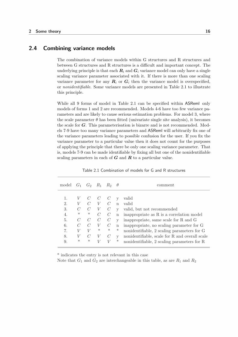
The combination of variance models within G structures and R structures andbetween G structures and R structures is a difficult and important concept. Theunderlying principle is that each Ri and Gi variance model can only have a singlescaling variance parameter associated with it. If there is more than one scalingvariance parameter for any Ri or Gi then the variance model is overspecified,or nonidentifiable. Some variance models are presented in Table 2.1 to illustratethis principle.

While all 9 forms of model in Table 2.1 can be specified within ASReml onlymodels of forms 1 and 2 are recommended. Models 4-6 have too few variance pa-rameters and are likely to cause serious estimation problems. For model 3, wherethe scale parameter θ has been fitted (univariate single site analysis), it becomesthe scale for G. This parameterisation is bizarre and is not recommended. Mod-els 7-9 have too many variance parameters and ASReml will arbitrarily fix one ofthe variance parameters leading to possible confusion for the user. If you fix thevariance parameter to a particular value then it does not count for the purposesof applying the principle that there be only one scaling variance parameter. Thatis, models 7-9 can be made identifiable by fixing all but one of the nonidentifiablescaling parameters in each of G and R to a particular value.

Table 2.1 Combination of models for G and R structures

model G1 G2 R1 R2 θ comment

1. V C C C y valid2. V C V C n valid3. C C V C y valid, but not recommended4. * * C C n inappropriate as R is a correlation model5. C C C C y inappropriate, same scale for R and G6. C C V C n inappropriate, no scaling parameter for G7. V V * * * nonidentifiable, 2 scaling parameters for G8. V C V C y nonidentifiable, scale for R and overall scale9. * * V V * nonidentifiable, 2 scaling parameters for R

* indicates the entry is not relevant in this caseNote that G1 and G2 are interchangeable in this table, as are R1 and R2

2 Some theory 17

2.5 Inference: Random effects

Tests of hypotheses: variance parameters

Inference concerning variance parameters of a linear mixed effects model usu-ally relies on approximate distributions for the (RE)ML estimates derived fromasymptotic results.

It can be shown that the approximate variance matrix for the REML estimates isgiven by the inverse of the expected information matrix (Cox and Hinkley, 1974,section 4.8). Since this matrix is not available in ASReml we replace the expectedinformation matrix by the AI matrix. Furthermore the REML estimates are con-sistent and asymptotically normal, though in small samples this approximationappears to be unreliable (see later).

A general method for comparing the fit of nested models fitted by REML is theREML likelihood ratio test, or REMLRT. The REMLRT is only valid if the fixedeffects are the same for both models. In ASReml this requires not only the samefixed effects model, but also the same parameterisation.

If `R2 is the REML log-likelihood of the more general model and `R1 is the REMLlog-likelihood of the restricted model (that is, the REML log-likelihood under thenull hypothesis), then the REMLRT is given by

D = 2 log(`R2/`R1) = 2 [log(`R2)− log(`R1)] (2.14)

which is strictly positive. If ri is the number of parameters estimated in modeli, then the asymptotic distribution of the REMLRT, under the restricted modelis χ2

r2−r1.

The REMLRT is implicitly two-sided, and must be adjusted when the test involvesan hypothesis with the parameter on the boundary of the parameter space. Infact, theoretically it can be shown that for a single variance component, say,the asymptotic distribution of the REMLRT is a mixture of χ2 variates, wherethe mixing probabilities are 0.5, one with 0 degrees of freedom (spike at 0) andthe other with 1 degree of freedom. The approximate P-value for the REMLRTstatistic (D), is 0.5(1-Pr(χ2

1 ≤ d)) where d is the observed value of D. Thedistribution of the REMLRT for the test that k variance components are zero, ortests involved in random regressions, which involve both variance and covariancecomponents, involves a mixture of χ2 variates from 0 to k degrees of freedom.See Self and Liang (1987) for details.

Tests concerning variance components in generally balanced designs, such as the

2 Some theory 18

balanced one-way classification, can be derived from the usual analysis of vari-ance. It can be shown that the REMLRT for a variance component being zero isa monotone function of the F-statistic for the associated term.

To compare two (or more) non-nested models we can evaluate the Akaike Infor-mation Criteria (AIC) or the Bayesian Information Criteria (BIC) for each model.These are given by

AIC = −2`Ri + 2ti

BIC = −2`Ri + ti log ν (2.15)

where ti is the number of variance parameters in model i and ν = n − p is theresidual degrees of freedom. AIC and BIC are calculated for each model and themodel with the smallest value is chosen as the preferred model.

Diagnostics

In this section we will briefly review some of the diagnostics that have been im-plemented in ASReml for examining the adequacy of the assumed variance matrixfor either R or G structures, or for examining the distributional assumptions re-garding e or u. Firstly we note that the BLUP of the residual vector is givenby

e = y −Wβ

= RPy (2.16)

It follows that

E (e) = 0

var (e) = R−WC−1W ′

The matrix WC−1W ′ is the so-called ‘extended hat’ matrix. It is the linearmixed effects model analogue of X(X ′X)−1X ′ for ordinary linear models. Thediagonal elements are returned in the .yht file by ASReml .

The variogram has been suggested as a useful diagnostic for assisting with theidentification of appropriate variance models for spatial data (Cressie, 1991).Gilmour et al. (1997) demonstrate its usefulness for the identification of thesources of variation in the analysis of field experiments. If the elements of thedata vector (and hence the residual vector) are indexed by a vector of spatialcoordinates, si, i = 1, . . . , n, then the ordinates of the sample variogram aregiven by

vij =12

[ei(si)− ej(sj)]2 , i, j = 1, . . . , n; i 6= j

2 Some theory 19

The sample variogram reported by ASReml has two forms depending on whetherNew

the spatial coordinates represent a complete rectangular lattice (as typical of afield trial) or not. In the lattice case, the sample variogram is calculated from thetriple (lij1, lij2, vij) where lij1 = si1−sj1 and lij2 = si2−sj2 are the displacements.As there will be many vij with the same displacements, ASReml calculates themeans for each displacement pair lij1, lij2 either ignoring the signs (default) orseparately for same sign and opposite sign (!TWOWAY), after grouping the largerdisplacements: 9-10, 11-14, 15-20, .... The result is displayed as a perspectiveplot (see page 205) of the one or two surfaces indexed by absolute displacementgroup. In this case, the two directions may be on different scales.

Otherwise ASReml forms a variogram based on polar coordinates. It calculatesthe distance between points dij =

√l2ij1 + l2ij2 and an angle θij (−180 < θij < 180)

subtended by the line from (0, 0) to (lij1, lij2) with the x-axis. The angle can becalculated as θij = tan−1(lij1/lij2) choosing (0 < θij < 180) if lij2 > 0 and(−180 < θij < 0) if lij2 < 0. Note that the variogram has angular symmetryin that vij = vji, dij = dji and |θij − θji| = 180. The variogram presentedaverages the vij within 12 distance classes and 4, 6 or 8 sectors (selected usinga !VGSECTORS qualifier) centred on an angle of (i − 1) ∗ 180/s (i = 1, ...s). Afigure is produced which reports the trends in vij with increasing distance foreach sector.

ASReml also computes the variogram from predictors of random effects whichappear to have a variance structures defined in terms of distance. The variogramdetails are reported in the .res file.

2.6 Inference: Fixed effects

Introduction

Inference for fixed effects in linear mixed models introduces some difficulties.New

In general, the methods used to construct F -tests in analysis of variance andregression cannot be used for the diversity of applications of the general linearmixed model available in ASReml. One approach would be to use likelihood ratiomethods (see Welham and Thompson, 1997) although their approach is not easilyimplemented.

Wald-type test procedures are generally favoured for conducting tests concerningτ . The traditional Wald statistic to test the hypothesis H0 : Lτ = l for given

2 Some theory 20

L, r × p, and l, r × 1, is given by

W = (Lτ − l)′L(X ′H−1X)−1L′−1(Lτ − l) (2.17)

and asymptotically, this statistic has a chi-square distribution on r degrees offreedom. These are marginal tests, so that there is an adjustment for all otherterms in the fixed part of the model. It is also anti-conservative if p-values areconstructed because it assumes the variance parameters are known.

The small sample behaviour of such statistics has been considered by Kenwardand Roger (1997) in some detail. They presented a scaled Wald statistic, to-gether with an F -approximation to its sampling distribution which they showedperformed well in a range (though limited in terms of the range of variance modelsavailable in ASReml) of settings.

In the following we describe the facilities now available in ASReml for conductinginference concerning terms which are the in dense fixed effects model componentof the general linear mixed model. These facilities are not available for any termsin the sparse model. These include facilities for computing two types of Waldstatistics and partial implementation of the Kenward and Roger adjustments.

Incremental and Conditional Wald Statistics

The basic tool for inference is the Wald statistic defined in equation 2.17. ASRemlproduces a test of fixed effects, that reduces to an F-statistic in special cases, bydividing the Wald test, constructed with l = 0, by r, the numerator degreesof freedom. In this form it is possible to perform an approximate F test ifwe can deduce the denominator degrees of freedom. However, there are severalways L can be defined to construct a test for a particular model term, two ofwhich are available in ASReml. For balanced designs, these Wald F-statisticsare numerically identical to the F-tests obtained from the standard analysis ofvariance.

The first method for computing Wald statistics (for each term) is the so-called“incremental” form. For this method, Wald statistics are computed from anincremental sum of squares in the spirit of the approach used in classical regressionanalysis (see Searle, 1971). For example if we consider a very simple modelwith terms relating to the main effects of two qualitative factors A and B, givensymbolically by

y ∼ 1 + A + B

where the 1 represents the constant term (µ), then the incremental sums of

2 Some theory 21

squares for this model can be written as the sequence

R(1)R(A|1) = R(1, A)−R(1)

R(B|1, A) = R(1, A,B)−R(1,A)

where the R(·) operator denotes the reduction in the total sums of squares dueto a model containing its argument and R(·|·) denotes the difference between thereduction in the sums of squares for any pair of (nested) models. Thus R(B|1, A)represents the difference between the reduction in sums of squares between theso-called maximal “model”

y ∼ 1 + A + B

andy ∼ 1 + A

Implicit in these calculations is that

• we only compute Wald statistics for estimable functions (Searle, 1971, page408),

• all variance parameters are held fixed at the current REML estimates from themaximal model

In this example, it is clear that the incremental Wald statistics may not producethe desired test for the main effect of A, as in many cases we would like to producea Wald statistic for A based on

R(A|1, B) = R(1, A,B)−R(1,B)

The issue is further complicated when we invoke “marginality” considerations.The issue of marginality between terms in a linear (mixed) model has been dis-cussed in much detail by Nelder (1977). In this paper Nelder defines marginalityfor terms in a factorial linear model with qualitative factors, but later Nelder(1994) extended this concept to functional marginality for terms involving quan-titative covariates and for mixed terms which involve an interaction betweenquantitative covariates and qualitative factors. Referring to our simple illustra-tive example above, with a full factorial linear model given symbolically by

y ∼ 1 + A + B + A.B

then A and B are said to be marginal to A.B, and 1 is marginal to A and B. In athree way factorial model given by

y ∼ 1 + A + B + C + A.B + A.C + B.C + A.B.C

2 Some theory 22

the terms A, B, C, A.B, A.C and B.C are marginal to A.B.C. Nelder (1977, 1994)argues that meaningful and interesting tests for terms in such models can onlybe conducted for those tests which respect marginality relations. This philos-ophy underpins the following description of the second Wald statistic availablein ASReml, the so-called “conditional” Wald statistic. This method is invokedby placing !FCON on the datafile line. ASReml attempts to construct conditionalWald statistics for each term in the fixed dense linear model so that marginalityrelations are respected. As a simple example, for the three way factorial modelthe conditional Wald statistics would be computed as

Term Sums of Squares M code1 R(1) .

A R(A | 1,B,C,B.C) = R(1,A,B,C,B.C) - R(1,B,C,B.C) A

B R(B | 1,A,C,A.C) = R(1,A,B,C,A.C) - R(1,A,C,A.C) A

C R(C | 1,A,B,A.B) = R(1,A,B,C,A.B) - R(1,A,B,A.B) A

A.B R(A.B | 1,A,B,C,A.C,B.C) = R(1,A,B,C,A.B,A.C,B.C) - R(1,A,B,C,A.C,B.C) B

A.C R(A.C | 1,A,B,C,A.B,B.C) = R(1,A,B,C,A.B,A.C,B.C) - R(1,A,B,C,A.B,B.C) B

B.C R(B.C | 1,A,B,C,A.B,A.C) = R(1,A,B,C,A.B,A.C,B.C) - R(1,A,B,C,A.B,A.C) B

A.B.C R(A.B.C | 1,A,B,C,A.B,A.C,B.C) = R(1,A,B,C,A.B,A.C,B.C,A.B.C) -R(1,A,B,C,A.B,A.C,B.C) C

Of these the conditional Wald statistic for the 1, B.C and A.B.C terms would bethe same as the incremental Wald statistics produced using the linear model

y ∼ 1 + A + B + C + A.B + A.C + B.C + A.B.C

The preceeding table includes a so-called M (marginality) code reported by ASRemlwhen conditional Wald statistics are presented. All terms with the highest M codeletter are tested conditionally on all other terms in the model, i.e. by droppingthe term from the maximum model. All terms with the preceeding M code letter,are marginal to at least one term in a higher group, and so forth. For example,in the table, model term A.B has M code B because it is marginal to model termA.B.C and model term A has M code A because it is marginal to A.B, A.C andA.B.C. Model term mu (M code .) is a special case in that its test is conditionalon all covariates but no factors. Following is some ASReml output from the .aovtable which reports the terms in the conditional statistics.

Marginality pattern for F-con calculation-- Model terms --

Model Term DF 1 2 3 4 5 6 7 8

1 mu 1 * . . . . . . .2 water 1 I * C C . . c .3 variety 7 I I * C . c . .4 sow 2 I I I * C . . .5 water.variety 7 I I I I * C C .

2 Some theory 23

6 water.sow 2 I I I I I * C .7 variety.sow 14 I I I I I I * .8 water.variety.sow 14 I I I I I I I *

F-inc tests the additional variation explained when the term (*) is added to amodel consisting of the I terms. F-con tests the additional variation explainedwhen the term (*) is added to a model consisting of the I and C/c terms. Anyc terms are ignored in calculating DenDF for F-con using numerical derivativesfor computational reasons. The . terms are ignored for both F-inc and F-contests.

Consider now a nested model which might be represented symbolically by

y ∼ 1 + REGION + REGION.SITE

For this model, the incremental and conditional Wald tests will be the same.However, it is not uncommon for this model to be presented to ASReml as

y ∼ 1 + REGION + SITE

with SITE identified across REGION rather than within REGION. Then the nestedstructure is hidden but ASReml will still detect the structure and produce a validconditional Wald F-statistic. This situation will be flagged in the M code field bychanging the letter to lower case. Thus, in the nested model, the three M codeswould be ., A and B because REGION.SITE is obviously an interaction dependenton REGION. In the second model, REGION and SITE appear to be independentfactors so the initial M codes are ., A and A. However they are not independentbecause REGION removes additional degrees of freedom from SITE, so the M codesare changed from ., A and A to ., a and A.

We strongly recommend, if you are in any doubt about the “maximal conditional”model (MCM) for the conditional Wald F-statistic, that you consult the .aov filewhich spells out the “maximal conditional” model for each term. We also adviseusers that the aim of the conditional Wald statistic is to facilitate inference forfixed effects. It is not meant to be prescriptive nor is it foolproof for every setting.

The Wald statistics are collectively presented in a summary table in the .asrfile. The basic table includes the numerator degrees of freedom (ν1i) and theincremental Wald F-statistic for each term. To this is added the conditionalWald F-statistic and the M code if !FCON is specified. A conditional F-statistic isnot reported for mu in the .asr but is in the .aov file (adjusted for covariates).

2 Some theory 24

Kenward and Roger Adjustments

In moderately sized analyses, ASReml will also include the denominator degreesof freedom (DenDF, denoted by ν2i, Kenward and Roger, 1997) and a probablityvalue if these can be computed. They will be for the conditional Wald F-statisticif it is reported. The !DDF i (see page 68) qualifier can be used to suppress theDenDF calculation (!DDF -1) or request a particular algorithmic method: !DDF1 for numerical derivatives, !DDF 2 for algebraic derivatives. The value in theprobability column (either P inc or P con) is computed from an Fν1i,ν2i referencedistribution. An approximation is used for computational convenience when cal-culating the DenDF for Conditional F statistics using numerical derivatives. TheDenDF reported then relates to a maximal conditional incremental model (MCIM)which, depending on the model order, may not always coincide with the max-imal conditional model (MCM) under which the conditional F statistic is cal-culated. The MCIM model omits terms fitted after any terms ignored for theconditional test (I after . in marginality pattern). In the example above, MCIMignores variety.sow when calculating DenDF for the test of water and ignoreswater.sow when calculating DenDF for the test of variety. When DenDF is notavailable, it is often possible, though anti-conservative to use the residual degreesof freedom for the denominator.

Kenward and Roger (1997) pursued the concept of construction of Wald-type teststatistics through an adjusted variance matrix of τ . They argued that it is usefulto consider an improved estimator of the variance matrix of τ which has less biasand accounts for the variability in estimation of the variance parameters. Thereare two reasons for this. Firstly, the small sample distribution of Wald tests issimplified when the adjusted variance matrix is used. Secondly, if measures ofprecision are required for τ or effects therein, those obtained from the adjustedvariance matrix will generally be preferred. Unfortunately the Wald statistics arecurrently computed using an unadjusted variance matrix.

Approximate stratum variances

ASReml reports approximate stratum variances and degrees of freedom for sim-ple variance components models. For the linear mixed-effects model with vari-ance components (setting σ2

H= 1) where G = ⊕q

j=1γjIbj , it is often possibleto consider a natural ordering of the variance component parameters includingσ2. Based on an idea due to Thompson (1980), ASReml computes approximatestratum degrees of freedom and stratum variances by a modified Cholesky diag-onalisation of the average information matrix. That is, if F is the average infor-mation matrix for σ, let U be an upper triangular matrix such that F = U ′U .

2 Some theory 25

We defineU c = DcU

where Dc is a diagonal matrix whose elements are given by the inverse elementsof the last column of U ie dcii = 1/uir, i = 1, . . . , r. The matrix U c is thereforeupper triangular with the elements in the last column equal to one. If the vectorσ is ordered in the “natural” way, with σ2 being the last element, then we candefine the vector of so called “pseudo” stratum variance components by

ξ = U cσ

Thencevar (ξ) = D2

c

The diagonal elements can be manipulated to produce effective stratum degreesof freedom Thompson (1980) viz

νi = 2ξ2i /d2

cii

In this way the closeness to an orthogonal block structure can be assessed.

3 A guided tour

Introduction

Nebraska Intrastate Nursery (NIN) field experiment

The ASReml data file

The ASReml command file

The title lineReading the dataThe data file line

Specifying the terms in the mixed modelTabulationPrediction

Variance structures

Running the job

Description of output files

The .asr fileThe .sln fileThe .yht file

Tabulation, predicted values and functions of the variancecomponents

26

3 A guided tour 27

3.1 Introduction

This chapter presents a guided tour of ASReml, from data file preparation andbasic aspects of the ASReml command file, to running an ASReml job and inter-preting the output files. You are encouraged to read this chapter before movingto the later chapters;

• a real data example is used in this chapter for demonstration, see below,

• the same data are also used in later chapters,

• links to the formal discussion of topics are clearly signposted by margin notes.

Note that some aspects of ASReml, in particular, pedigree files (see Chapter 9)and multivariate analysis (see Chapter 8) are only covered in later chapters.

ASReml is essentially a batch program with some optional interactive features.The typical sequence of operations when using ASReml is

• Prepare the data (typically using a spreadsheet or data base program)

• Export that data as an ASCII file (for example export it as a .csv (commaseparated values) file from Excel)

• Prepare a job file with filename extension .as.

• Run the job file with ASReml

• Review the various output files

• revise the job and re run it, or

• extract pertinant results for your report.

You will need a file editor to create the command file and to view the variousoutput files. On unix systems, vi and emacs are commonly used. Under Win-dows, there are several suitable program editors available such as ASReml-W andConText described in section 1.3.New

3.2 Nebraska Intrastate Nursery (NIN) field experiment

The yield data from an advanced Nebraska Intrastate Nursery (NIN) breedingtrial conducted at Alliance in 1988/89 will be used for demonstration, see Stroupet al. (1994) for details. Four replicates of 19 released cultivars, 35 experimen-tal wheat lines and 2 additional triticale lines were laid out in a 22 row by 11

3 A guided tour 28

column rectangular array of plots; the varieties were allocated to the plots usinga randomised complete block (RCB) design. In field trials, complete replicatesare typically allocated to consecutive groups of whole columns or rows. In thistrial the replicates were not allocated to groups of whole columns, but rather,overlapped columns. Table 3.1 gives the allocation of varieties to plots in fieldplan order with replicates 1 and 3 in ITALICS and replicates 2 and 4 in BOLD.

3.3 The ASReml data file

The standard format of an ASReml data file is to have the data arranged inSee Chapter 4

for details space, TAB or comma separated columns/fields with a line for each samplingunit. The columns contain covariates, factors, response variates (traits) andweight variables in any convenient order. This is the first 30 lines of the filenin89.asd containing the data for the NIN variety trial. The data are in fieldorder (rows within columns) and an optional heading (first line of the file) hasbeen included to document the file. In this case there are 11 space separated datafields (variety. . . column) and the complete file has 224 data lines, one for eachvariety in each replicate.

variety id pid raw repl nloc yield lat long row column

LANCER 1 1101 585 1 4 29.25 4.3 19.2 16 1

BRULE 2 1102 631 1 4 31.55 4.3 20.4 17 1

REDLAND 3 1103 701 1 4 35.05 4.3 21.6 18 1

CODY 4 1104 602 1 4 30.1 4.3 22.8 19 1

ARAPAHOE 5 1105 661 1 4 33.05 4.3 24 20 1

NE83404 6 1106 605 1 4 30.25 4.3 25.2 21 1

NE83406 7 1107 704 1 4 35.2 4.3 26.4 22 1

NE83407 8 1108 388 1 4 19.4 8.6 1.2 1 2

CENTURA 9 1109 487 1 4 24.35 8.6 2.4 2 2

SCOUT66 10 1110 511 1 4 25.55 8.6 3.6 3 2

COLT 11 1111 502 1 4 25.1 8.6 4.8 4 2

NE83498 12 1112 492 1 4 24.6 8.6 6 5 2

NE84557 13 1113 509 1 4 25.45 8.6 7.2 6 2

NE83432 14 1114 268 1 4 13.4 8.6 8.4 7 2

NE85556 15 1115 633 1 4 31.65 8.6 9.6 8 2

NE85623 16 1116 513 1 4 25.65 8.6 10.8 9 2

CENTURAK78 17 1117 632 1 4 31.6 8.6 12 10 2

NORKAN 18 1118 446 1 4 22.3 8.6 13.2 11 2

KS831374 19 1119 684 1 4 34.2 8.6 14.4 12 2...

optional field labelsdata line sampling unit 1data line sampling unit 2

.

.

.

Note that in Chapter 7 these data are analysed using spatial methods of analysis,see model 3a in Section 7.3. For spatial analysis using a separable error structure

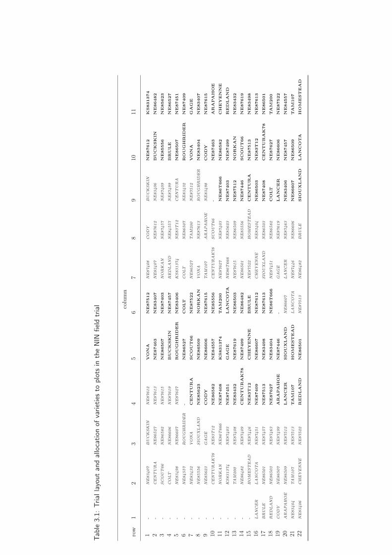
Tab

le3.

1:Trial

layo

ut

and

allo

cation

ofva

riet

ies

toplo

tsin

the

NIN

fiel

dtr

ial colu

mn

row

12

34

56

78

910

11

1-

NE83407

BU

CK

SK

INN

E87612

VO

NA

NE87512

NE87408

CO

DY

BU

CK

SK

INN

E87612

KS831374

2-

CEN

TU

RA

NE86527

NE87613

NE87463

NE83407

NE83407

NE87612

NE83406

BU

CK

SK

IN

NE86482

3-

SCO

UT66

NE86582

NE87615

NE86507

NE87403

NO

RK

AN

NE87457

NE87409

NE85556

NE85623

4-

CO

LT

NE86606

NE87619

BU

CK

SK

IN

NE87457

RED

LA

ND

NE84557

NE87499

BR

ULE

NE86527

5-

NE83498

NE86607

NE87627

RO

UG

HR

ID

ER

NE83406

KS831374

NE83T12

CEN

TU

RA

NE86507

NE87451

6-

NE84557

RO

UG

HR

IDER

-N

E86527

CO

LT

CO

LT

NE86507

NE83432

RO

UG

HR

ID

ER

NE87409

7-

NE83432

VO

NA

CEN

TU

RA

SC

OU

T66

NE87522

NE86527

TA

M200

NE87512

VO

NA

GA

GE

8-

NE85556

SIO

UX

LA

ND

NE85623

NE86509

NO

RK

AN

VO

NA

NE87613

RO

UG

HR

IDER

NE83404

NE83407

9-

NE85623

GAG

EC

OD

YN

E86606

NE87615

TA

M107

AR

APA

HO

EN

E83498

CO

DY

NE87615

10

-CEN

TU

RA

K78

NE83T12

NE86582

NE84557

NE85556

CEN

TU

RA

K78

SCO

UT66

-N

E87463

AR

APA

HO

E

11

-N

OR

KA

NN

E86T666

NE87408

KS831374

TA

M200

NE87627

NE87403

NE86T

666

NE86582

CH

EY

EN

NE

12

-K

S831374

NE87403

NE87451

GA

GE

LA

NC

OTA

NE86T666

NE85623

NE87403

NE87499

RED

LA

ND

13

-TA

M200

NE87408

NE83432

NE87619

NE86503

NE87615

NE86509

NE87512

NO

RK

AN

NE83432

14

-N

E86482

NE87409

CEN

TU

RA

K78

NE87499

NE86482

NE86501

NE85556

NE87446

SC

OU

T66

NE87619

15

-H

OM

ESTEA

DN

E87446

NE83T

12

CH

EY

EN

NE

BR

ULE

NE87522

HO

MESTEA

DC

EN

TU

RA

NE87513

NE83498

16

LA

NCER

LA

NCO

TA

NE87451

NE87409

NE86607

NE87612

CH

EY

EN

NE

NE83404

NE86503

NE83T

12

NE87613

17

BRU

LE

NE86501

NE87457

NE87513

NE83498

NE87613

SIO

UX

LA

ND

NE86503

NE87408

CEN

TU

RA

K78

NE86501

18

RED

LA

ND

NE86503

NE87463

NE87627

NE83404

NE86T

666

NE87451

NE86582

CO

LT

NE87627

TA

M200

19

CO

DY

NE86507

NE87499

AR

APA

HO

EN

E87446

-G

AG

EN

E87619

LA

NC

ER

NE86606

NE87522

20

AR

APA

HO

EN

E86509

NE87512

LA

NC

ER

SIO

UX

LA

ND

NE86607

LA

NCER

NE87463

NE83406

NE87457

NE84557

21

NE83404

TA

M107

NE87513

TA

M107

HO

MEST

EA

DLA

NCO

TA

NE87446

NE86606

NE86607

NE86509

TA

M107

22

NE83406

CH

EY

EN

NE

NE87522

RED

LA

ND

NE86501

NE87513

NE86482

BRU

LE

SIO

UX

LA

ND

LA

NC

OTA

HO

MEST

EA

D

3 A guided tour 30

(see Chapter 2) the data file must first be augmented to specify the complete 22row × 11 column array of plots. These are the first 20 lines of the augmenteddata file nin89aug.asd with 242 data rows.

variety id pid raw repl nloc yield lat long row column

LANCER 1 NA NA 1 4 NA 4.3 1.2 1 1

LANCER 1 NA NA 1 4 NA 4.3 2.4 2 1

LANCER 1 NA NA 1 4 NA 4.3 3.6 3 1

LANCER 1 NA NA 1 4 NA 4.3 4.8 4 1

LANCER 1 NA NA 1 4 NA 4.3 6 5 1

LANCER 1 NA NA 1 4 NA 4.3 7.2 6 1

LANCER 1 NA NA 1 4 NA 4.3 8.4 7 1

LANCER 1 NA NA 1 4 NA 4.3 9.6 8 1

LANCER 1 NA NA 1 4 NA 4.3 10.8 9 1

LANCER 1 NA NA 1 4 NA 4.3 12 10 1

LANCER 1 NA NA 1 4 NA 4.3 13.2 11 1

LANCER 1 NA NA 1 4 NA 4.3 14.4 12 1

LANCER 1 NA NA 1 4 NA 4.3 15.6 13 1

LANCER 1 NA NA 1 4 NA 4.3 16.8 14 1

LANCER 1 NA NA 1 4 NA 4.3 18 15 1

LANCER 1 NA NA 2 4 NA 17.2 7.2 6 4

LANCER 1 NA NA 3 4 NA 25.8 22.8 19 6

LANCER 1 NA NA 4 4 NA 38.7 12.0 10 9

LANCER 1 1101 585 1 4 29.25 4.3 19.2 16 1

BRULE 2 1102 631 1 4 31.55 4.3 20.4 17 1

REDLAND 3 1103 701 1 4 35.05 4.3 21.6 18 1

CODY 4 1104 602 1 4 30.1 4.3 22.8 19 1...

optional field labelsfile augmented bymissing values for first15 plots and 3 bufferplots and variety codedLANCER to complete22×11 array...

buffer plotsbetween reps

original data...

Note that

• the pid, raw, repl and yield data for the missing plots have all been madeNA (one of the three missing value indicators in ASReml, see Section 4.2),

• variety is coded LANCER for all missing plots; one of the variety names mustbe used but the particular choice is arbitrary.

3.4 The ASReml command file

By convention an ASReml command file has a .as extension. The file definesSee Chapters 5,

6 and 7 for de-

tails• a title line to describe the job,

• labels for the data fields in the data file and the name of the data file,

• the linear mixed model and the variance model(s) if required,

• output options including directives for tabulation and prediction.

3 A guided tour 31

Below is the ASReml command file for an RCB analysis of the NIN field trial datahighlighting the main sections. Note the order of the main sections.

title line −→data field definition−→

.

.

.

data field definition −→data file name and qualifiers−→

tabulate statement−→linear mixed model definition−→

predict statement−→variance model specification−→

.

.

NIN Alliance trial 1989

variety !A

id

pid

raw

repl 4

nloc

yield

lat

long

row 22

column 11

nin89.asd !skip 1

tabulate yield ∼ variety

yield ∼ mu variety !r repl

predict variety

0 0 1

repl 1

repl 0 IDV 0.1

The title line

NIN Alliance trial 1989

variety !A

id...

The first non-blank line in an ASReml com-mand file is taken as the title for the job andis used to identify the analysis for future ref-erence.

Reading the data

NIN Alliance trial 1989

variety !A

id

pid

raw

repl 4

nloc

yield

lat

long

row 22

column 11

nin89.asd !skip 1...

The data fields are defined before the data filename is specified. Field definitions must begiven for all fields in the data file and in theorder in which they appear in the data file.Data field definitions must be indented.In this case there are 11 data fields (variety. . . column) in nin89.asd, see Section 3.3.

The !A after variety tells ASReml that thefirst field is alphanumeric and the 4 after repltells ASReml that the field called repl (thefifth field read) is a numeric factor with 4 lev-

3 A guided tour 32

els. Similarly for row and column. The otherdata fields include variates (yield) and various other variables.

The data file line

NIN Alliance trial 1989

variety !A

id

pid...

row 22

column 11

nin89.asd !skip 1

tabulate yield ∼ variety

yield ∼ mu variety !r repl

predict variety

0 0 1

repl 1

repl 0 IDV 0.1

The data file name is specified immediatelyafter the last data field definition. Data filequalifiers that relate to data input and outputare also placed on this line if they are required.In this example, !skip 1 tells ASReml to readSee Section 5.7

the data from nin89.asd but to ignore thefirst line in this file, the line containing thefield labels.

The data file line can also contain qualifiersSee Section 5.8

that control other aspects of the analysis.These qualifiers are presented in Section 5.8.

Tabulation

...

column 11

nin89.asd !skip 1

tabulate yield ∼ variety

yield ∼ mu variety !r repl

predict variety...

Tabulate statements provide a simple way ofSee Chapter 10

exploring the structure of a data file. They ap-pear immediately before (or after) the modelline. In this case the 56 simple variety meansfor yield are formed and written to a .taboutput file. See Chapter 10 for a discussion oftabulation.

Specifying the terms in the mixed model

NIN Alliance trial 1989

variety !A...

column 11

nin89.asd !skip 1

tabulate yield ∼ variety

yield ∼ mu variety !r repl

predict variety

0 0 1

repl 1

repl 0 IDV 0.1

The linear mixed model is specified as a list ofSee Chapter 6

model terms and qualifiers. All elements mustbe space separated. ASReml accommodates awide range of analyses. See Section 2.1 for abrief discussion and general algebraic formu-lation of the linear mixed model. The modelspecified here for the NIN data is a simple ran-dom effects RCB model including fixed vari-ety effects and random replicate effects. Thereserved word mu fits a constant term (inter-

3 A guided tour 33

cept), variety fits a fixed variety effect and repl fits a random replicate effect.The !r qualifier tells ASReml to fit the terms that appear after this qualifier asrandom effects.

Prediction

NIN Alliance trial 1989

variety !A...

column 11

nin89.asd !skip 1

tabulate yield ∼ variety

yield ∼ mu variety !r repl

predict variety

0 0 1

repl 1

repl 0 IDV 0.1

Prediction statements appear after the modelSee Chapter 10

statement and before any variance structurelines. In this case the 56 variety means foryield would be formed and returned in the.pvs output file. See Chapter 10 for a de-tailed discussion of prediction in ASReml.

Variance structures

NIN Alliance trial 1989

variety !A...

column 11

nin89.asd !skip 1

tabulate yield ∼ variety

yield ∼ mu variety !r repl

predict variety

0 0 1

repl 1

repl 0 IDV 0.1

The last three lines are included for exposi-tory purposes and are not actually needed forthis analysis. An extensive range of varianceSee Chapter 7

structures can be fitted in ASReml. See Chap-ter 7 for a lengthy discussion of variance mod-elling in ASReml. In this case independentand identically distributed random replicateeffects are specified using the identifier IDV ina G structure. G structures are described inSection 2.1 and the list of available variancestructures/models is presented in Table 7.3. Since IDV is the default variancestructure for random effects, the same analysis would be performed if these lineswere omitted.

3.5 Running the job

An ASReml job is often run from a command line. The basic command to runSee Chapter 12

an ASReml job is normally

asreml basename[.as]

where basename[.as] is the name of the command file. For example, the com-

3 A guided tour 34

mand to run nin89.as is

asreml nin89.as

However, if the path to ASReml is not specified in your system’s Path envi-ronment variable, a path to this program must also be given. In this case thecommand to run the ASReml job in a PC/Windows environment is

[path]asreml basename[.as]

where path is typically C:\Program Files\ASReml2\bin\ pointing to the locationof the ASReml program. In this guide we assume the command file has a filenameMake a habit of

giving command

files the .as ex-

tension

extension .as. ASReml also recognises the filename extension .asc as an ASReml

command file. When these are used, the extension (.as or .asc) may be omittedfrom basename.as in the command line if there is no file in the working directorywith the name basename. The options and arguments that can be supplied onthe command line to modify a job at run time are described in Chapter 12.

Forming a job template

Notice that the data files nin89.asd and nin89aug.asd commenced with a lineNew

of column headings. Since these headings do not contain embedded blanks, wecan use ASReml to make a template for the .as file by running ASReml with thedatafile as the command argument (see Chapter 12). For example, running thecommand

asreml nin89aug.asd

writes a file nin89aug.as (if it does not already exist) which looks like

Title: nin89aug.

#variety id pid raw rep nloc yield lat long row column

#LANCER 1 NA NA 1 4 NA 4.3 1.2 1 1

#LANCER 1 NA NA 1 4 NA 4.3 2.4 2 1

#LANCER 1 NA NA 1 4 NA 4.3 3.6 3 1

#LANCER 1 NA NA 1 4 NA 4.3 4.8 4 1

variety !A

id *

pid

raw

rep *

nloc *

yield

lat

long

row *

column *

# Check/Correct these field definitions.

nin89aug.asd !SKIP 1

3 A guided tour 35

column ~ mu , # Specify fixed model

!r # Specify random model

# 1 2 0

# column column AR1 0.1

# row row AR1 0.1

This is a template in that it needs editing (it has nominated an inappropriateresponse variable) but it displays the first few lines of the data and infers whetherfields are factors or variates as follows: Missing fields and those with decimalpoints in the data value are taken as covariates, integer fields are taken as simplefactors (*) and alphanumeric fields are taken as !A factors.

3.6 Description of output files

A series of output files are produced with each ASReml run. Running the exam-ple as above, the primary output is written to nin89.asr. This file contains asummary of the data, the iteration sequence, estimates of the variance parame-ters and an analysis of variance (ANOVA) table. The estimates of all the fixedand random effects are written to nin89.sln. The residuals, predicted values ofthe observations and the diagonal elements of the hat matrix (see Chapter 2) arereturned in nin89.yht, see Section 13.3. Other files produced by this job includethe .aov, .pvs, .res, .tab, .vvp and .veo files, see Section 13.4.

The .asr file

Below is nin89.asr with pointers to the main sections. The first line gives theversion of ASReml used (in square brackets) and the title of the job. The secondline gives the build date for the program and indicates whether it is a 32bit or64bit version. The third line gives the date and time that the job was run andreports the size of the workspace. The general announcements box (outlined inasterisks) at the top of the file notifies the user of current release features. Theremaining lines report a data summary, the iteration sequence, the estimatedvariance parameters and an ANOVA table. The final line gives the date and timethat the job was completed and a statement about convergence.

ASReml 1.63o [01 Jun 2005] NIN alliance trial 1989job heading

Build: j [01 Jul 2005] 32 bit

11 Jul 2005 13:55:21.504 32.00 Mbyte Windows nin89

Licensed to: Arthur Gilmournotices

***********************************************************

3 A guided tour 36

* SYNTAX change: A/B now means A A.B *

* *

* Contact support@asreml.co.uk for licensing and support *

***************************************************** ARG *

Folder: C:\data\asr\UG2\manex

variety !A

QUALIFIERS: !SKIP 1

Reading nin89.asd FREE FORMAT skipping 1 linesdata summary

Univariate analysis of yield

Using 224 records of 224 read

Model term Size #miss #zero MinNon0 Mean MaxNon0

1 variety 56 0 0 1 28.5000 56

2 id 0 0 1.000 28.50 56.00

3 pid 0 0 1101. 2628. 4156.

4 raw 0 0 21.00 510.5 840.0

5 repl 4 0 0 1 2.5000 4

6 nloc 0 0 4.000 4.000 4.000

7 yield Variate 0 0 1.050 25.53 42.00

8 lat 0 0 4.300 27.22 47.30

9 long 0 0 1.200 14.08 26.40

10 row 22 0 0 1 11.7321 22

11 column 11 0 0 1 6.3304 11

12 mu 1

4 identity 0.1000

Structure for repl has 4 levels defined

Forming 61 equations: 57 dense.

Initial updates will be shrunk by factor 0.316

NOTICE: 1 singularities detected in design matrix.

1 LogL=-454.807 S2= 50.329 168 df 1.000 0.1000iteration

2 LogL=-454.663 S2= 50.120 168 df 1.000 0.1173sequence

3 LogL=-454.532 S2= 49.868 168 df 1.000 0.1463

4 LogL=-454.472 S2= 49.637 168 df 1.000 0.1866

5 LogL=-454.469 S2= 49.585 168 df 1.000 0.1986

6 LogL=-454.469 S2= 49.582 168 df 1.000 0.1993

7 LogL=-454.469 S2= 49.582 168 df 1.000 0.1993

Final parameter values 1.0000 0.19932

Source Model terms Gamma Component Comp/SE % C

3 A guided tour 37

Variance 224 168 1.00000 49.5824 9.08 0 Pparameter

repl identity 4 0.199323 9.88291 1.12 0 Uestimates

Analysis of Variance NumDF DenDF F_inc ProbANOVA

12 mu 1 3.0 242.05 <.001

1 variety 55 165.0 0.88 0.708

Notice: The DenDF values are calculated ignoring fixed/boundary/singular

variance parameters using algebraic derivatives.

5 repl 4 effects fitted

Finished: 11 Jul 2005 13:55:25.309 LogL Converged

The .sln file

The following is an extract from nin89.sln containing the estimated varietyeffects, intercept and random replicate effects in this order (column 3) with stan-dard errors (column 4). Note that the variety effects are returned in the order oftheir first appearance in the data file, see replicate 1 in Table 3.1.

variety LANCER 0.000 0.000

variety BRULE -2.487 4.979

variety REDLAND 1.938 4.979

variety CODY -7.350 4.979

variety ARAPAHOE 0.8750 4.979

variety NE83404 -1.175 4.979

variety NE83406 -4.287 4.979

variety NE83407 -5.875 4.979

variety CENTURA -6.912 4.979

variety SCOUT66 -1.037 4.979

variety COLT -1.562 4.979

variety NE83498 1.563 4.979

variety NE84557 -8.037 4.979

variety NE83432 -8.837 4.979...

variety NE87615 -2.875 4.979

variety NE87619 2.700 4.979

variety NE87627 -5.337 4.979

mu 1 28.56 3.856

repl 1 1.880 1.755

repl 2 2.843 1.755

3 A guided tour 38

repl 3 -0.8713 1.755

repl 4 -3.852 1.755

The .yht file

The following is an extract from nin89.yht containing the predicted values ofthe observations (column 2), the residuals (column 3) and the diagonal elementsof the hat matrix. This final column can be used in tests involving the residuals,see Section 2.5 under Diagnostics.

Record Yhat Residual Hat

1 30.442 -1.192 13.01

2 27.955 3.595 13.01

3 32.380 2.670 13.01

4 23.092 7.008 13.01

5 31.317 1.733 13.01

6 29.267 0.9829 13.01

7 26.155 9.045 13.01

8 24.567 -5.167 13.01

9 23.530 0.8204 13.01...

222 16.673 9.877 13.01

223 24.548 1.052 13.01

224 23.786 3.114 13.01

3.7 Tabulation, predicted values and functions of the variance com-ponents

It may take several runs of ASReml to determine an appropriate model for thedata, that is, the fixed and random effects that are important. During thisprocess you may wish to explore the data by simple tabulation. Having identifiedan appropriate model, you may then wish to form predicted values or functionsof the variance components. The facilities in ASReml to form predicted valuesand functions of the variance components are described in Chapters 10 and 11respectively. Our example only includes tabulation and prediction.

The statement

tabulate yield ∼ variety

3 A guided tour 39

in nin89.as results in nin89.tab as follows:

NIN alliance trial 1989 11 Jul 2005 13:55:21

Simple tabulation of yield

variety

LANCER 28.56

BRULE 26.07

REDLAND 30.50

CODY 21.21

ARAPAHOE 29.44

NE83404 27.39

NE83406 24.28

NE83407 22.69

CENTURA 21.65

SCOUT66 27.52

COLT 27.00...

NE87522 25.00

NE87612 21.80

NE87613 29.40

NE87615 25.69

NE87619 31.26

NE87627 23.23

The

predict variety

statement after the model statement in nin89.as results in the nin89.pvs filedisplayed below (some output omitted) containing the 56 predicted variety means,also in the order in which they first appear in the data file (column 2), togetherwith standard errors (column 3). An average standard error of difference amongthe predicted variety means is displayed immediately after the list of predictedvalues. As in the .asr file, date, time and trial information are given the title line.The Ecode for each prediction (column 4) is usually E indicating the prediction isof an estimable function. Predictions of non-estimable functions are usually notprinted, see Chapter 10.

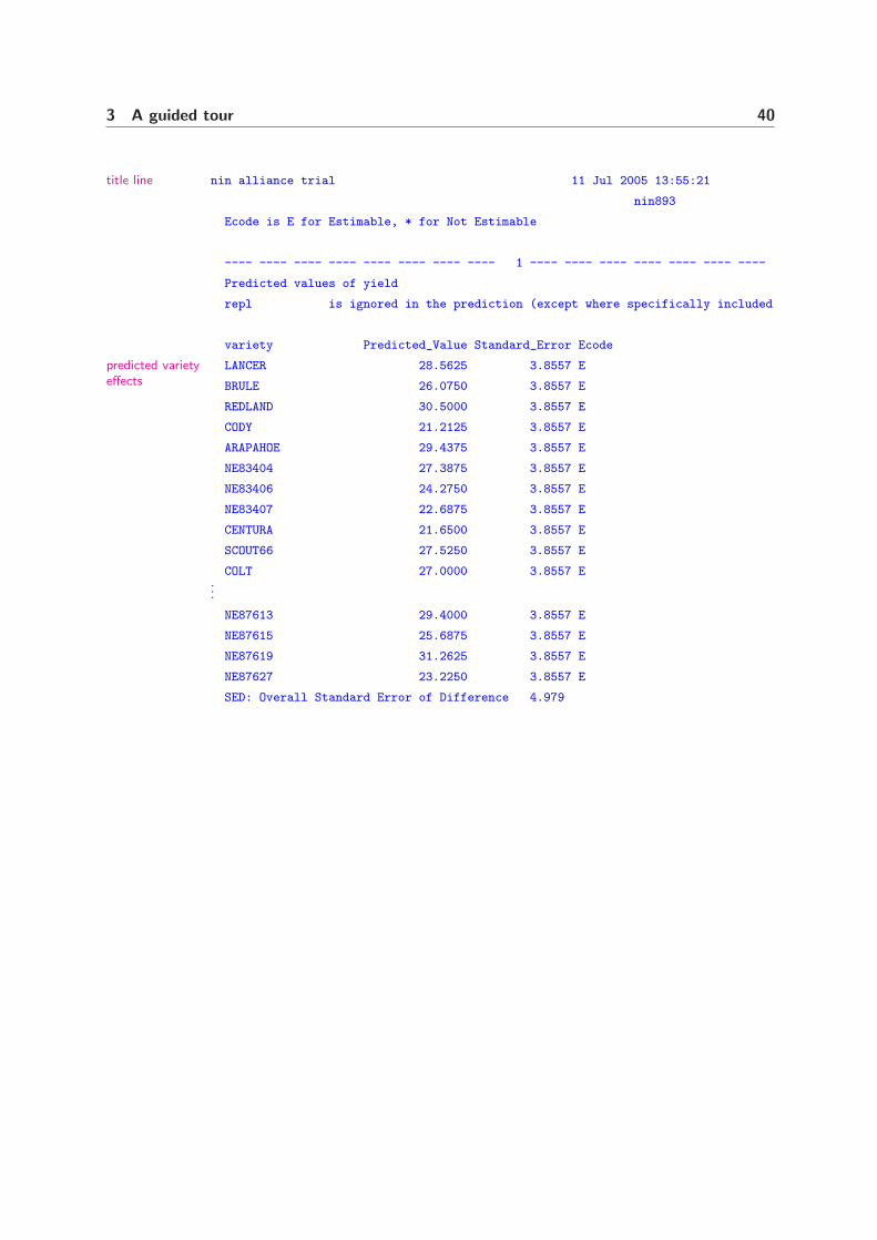
3 A guided tour 40

nin alliance trial 11 Jul 2005 13:55:21title line

nin893

Ecode is E for Estimable, * for Not Estimable

---- ---- ---- ---- ---- ---- ---- ---- 1 ---- ---- ---- ---- ---- ---- ----

Predicted values of yield

repl is ignored in the prediction (except where specifically included

variety Predicted_Value Standard_Error Ecode

LANCER 28.5625 3.8557 Epredicted varietyeffects BRULE 26.0750 3.8557 E

REDLAND 30.5000 3.8557 E

CODY 21.2125 3.8557 E

ARAPAHOE 29.4375 3.8557 E

NE83404 27.3875 3.8557 E

NE83406 24.2750 3.8557 E

NE83407 22.6875 3.8557 E

CENTURA 21.6500 3.8557 E

SCOUT66 27.5250 3.8557 E

COLT 27.0000 3.8557 E...

NE87613 29.4000 3.8557 E

NE87615 25.6875 3.8557 E

NE87619 31.2625 3.8557 E

NE87627 23.2250 3.8557 E

SED: Overall Standard Error of Difference 4.979

4 Data file preparation

Introduction

The data file

Free formatFixed format

Preparing data files in ExcelBinary format

41

4 Data file preparation 42

4.1 Introduction

The first step in an ASReml analysis is to prepare the data file. Data file prepara-tion is described in this chapter using the NIN example of Chapter 3 for demon-stration. The first 25 lines of the data file are as follows:

variety id pid raw repl nloc yield lat long row column

BRULE 2 1102 631 1 4 31.55 4.3 20.4 17 1

REDLAND 3 1103 701 1 4 35.05 4.3 21.6 18 1

CODY 4 1104 602 1 4 30.1 4.3 22.8 19 1

ARAPAHOE 5 1105 661 1 4 33.05 4.3 24 20 1

NE83404 6 1106 605 1 4 30.25 4.3 25.2 21 1

NE83406 7 1107 704 1 4 35.2 4.3 26.4 22 1

NE83407 8 1108 388 1 4 19.4 8.6 1.2 1 2

CENTURA 9 1109 487 1 4 24.35 8.6 2.4 2 2

SCOUT66 10 1110 511 1 4 25.55 8.6 3.6 3 2

COLT 11 1111 502 1 4 25.1 8.6 4.8 4 2

NE83498 12 1112 492 1 4 24.6 8.6 6 5 2

NE84557 13 1113 509 1 4 25.45 8.6 7.2 6 2

NE83432 14 1114 268 1 4 13.4 8.6 8.4 7 2

NE85556 15 1115 633 1 4 31.65 8.6 9.6 8 2

NE85623 16 1116 513 1 4 25.65 8.6 10.8 9 2

CENTURK78 17 1117 632 1 4 31.6 8.6 12 10 2

NORKAN 18 1118 446 1 4 22.3 8.6 13.2 11 2

KS831374 19 1119 684 1 4 34.2 8.6 14.4 12 2

TAM200 20 1120 422 1 4 21.1 8.6 15.6 13 2

NE86482 21 1121 560 1 4 28 8.6 16.8 14 2

HOMESTEAD 22 1122 566 1 4 28.3 8.6 18 15 2

LANCOTA 23 1123 514 1 4 25.7 8.6 19.2 16 2

NE86501 24 1124 635 1 4 31.75 8.6 20.4 17 2

NE86503 25 1125 840 1 4 42 8.6 21.6 18 2...

4.2 The data file

The standard format of an ASReml data file is to have the data arranged incolumns/fields with a single line for each sampling unit. The columns containvariates and covariates (numeric), factors (alphanumeric), traits (response vari-ables) and weight variables in any order that is convenient to the user. The datafile may be free format, fixed format or a binary file.

Free format data files

The data are read free format (space, comma or tab separated) unless the filename has extension .bin for real binary, or .dbl for double precision binary (see

4 Data file preparation 43

below). Important points to note are as follows:

• files prepared in Excel must be converted to comma or tab-delimited form.

• blank lines are ignored,

• column headings, field labels or comments may be present at the top of thefile provided that the !skip qualifier (Table 5.2) is used to skip over them,

• NA,* and . are treated as coding for missing values in free format data files;

– if missing values are coded with a unique data value (for example, 0 or -9),use !M to flag them as missing or !D to drop the data record containingthem (see Table 5.1),

• comma delimited files whose file name ends in .csv or for which the !CSVqualifier is set recognise empty fields as missing values,

– a line beginning with a comma implies a preceding missing value,– consecutive commas imply a missing value,– a line ending with a comma implies a trailing missing value,– if the filename does not end in .csv or the !CSV qualifier is not set, commas

are treated as white space,

• characters following # on a line are ignored so this character may not be usedin alphanumeric fields,

• blank spaces, tabs and commas must not be used (embedded) in alphanumericfields unless the label is enclosed in quotes, for example, the name WillowCreek would need to be appear in the data file as ‘Willow Creek’ to avoiderror,

• the $ symbol must not be used in the data file,

• alphanumeric fields have a default size of 16 characters. Use the !LL qualifierto extend the size of factor labels stored.New

• extra data fields on a line are ignored,

• if there are fewer data items on a line than ASReml expects the remainder aretaken from the following line(s) except in .csv files were they are taken asmissing. If you end up with half the number of records you expected, this isprobably the reason,

• all lines beginning with ! followed by a blank are copied to the .asr file ascomments for the output; their contents are ignored,

• a data file line may not exceed 2000 characters; if the data fields will not fit inNew

2000 characters, put some on the next line.

4 Data file preparation 44

Fixed format data files

The format must be supplied with the !FORMAT qualifier which is described in(Table 5.5). However, if all fields are present and are separated, the file can beread free format.

Preparing data files in Excel

Many users find it convenient to prepare their data in Excel or Access. How-ever, the data must be exported from these programs into either .csv (Commaseparated values) or .txt (TAB separated values) form for ASReml to read it.ASReml can convert an .xls file to a .csv file. When ASReml is invoked with an.xls file as the filename argument and there is no .csv file or .as with the samebasename, it exports the first sheet as a .csv file and then generates a template.as command file from any column headings it finds (see page 178). It will alsoconvert a Genstat .gsh spreadsheet file to .csv format. The data extracted fromthe .xls file are labels, numerical values and the results from formulae. Emptyrows at the start and end of a block are trimmed, but empty rows in the middleof a block are kept. Empty columns are ignored. A single row of labels as the firstnon-empty row in the block will be taken as column names. Empty cells in thisrow will have default names C1, C2 etc. assigned. Missing values are commonlyrepresented in ASReml data files by NA, * or .. ASReml will also recognise emptyfields as missing values in .csv (.xls) files.

Binary format data files

Conventions for binary files are as follows:

• binary files are read as unformatted Fortran binary in single precision if thefilename has a .bin or .BIN extension,

• Fortran binary data files are read in double precision if the filename has a .dblor .DBL extension,

• ASReml recognises the value -1e37 as a missing value in binary files,

• Fortran binary in the above means all real (.bin) or all double precision (.dbl)variables; mixed types, that is, integer and alphabetic binary representation ofvariables is not allowed in binary files,

• binary files can only be used in conjunction with a pedigree file if the pedigreefields are coded in the binary file so that they correspond with the pedigree file(this can be done using the !SAVE option in ASReml to form the binary file,see Table 5.5), or the identifiers are whole numbers less than 9,999,999 and the!RECODE qualifier is specified (see Table 5.5).

5 Command file: Reading the data

Introduction

Important rules

Title line

Specifying and reading the data

Data field definition syntax

Transforming the data

Transformation syntaxOther rules and examplesSpecial note on covariates

Other examples

Datafile line

Datafile line syntax

Datafile qualifiers

Job control qualifiers

45

5 Command file: Reading the data 46

5.1 Introduction

NIN Alliance Trial 1989

variety !A

id

pid

raw

repl 4

nloc

yield

lat

long

row 22

column 11

nin89aug.asd !skip 1

yield ∼ mu variety

1 2

11 column AR1 .424

22 row AR1 .904

In the code box to the right is the ASReml

command file nin89a.as for a spatial analysisof the Nebraska Intrastate Nursery (NIN) fieldexperiment introduced Chapter 3. The linesthat are highlighted in bold/blue type relateto reading in the data. In this chapter we usethis example to discuss reading in the data indetail.

5.2 Important rules

In the ASReml command file

• all characters following a # symbol on a line are ignored,

• all blank lines are ignored,

• lines beginning with ! followed by a blank are copied to the .asr file ascomments for the output,

• a blank is the usual separator; tab is also a separator,

• maximum line length is 2000 characters,New

• a comma as the last character on the line is used to indicate that the currentlist is continued on the next line; a comma is not needed when ASReml knowshow many values to read,

• reserved words used in specifying the linear model (Table 6.1) are case sensitive;they need to be typed exactly as defined: they may not be abbreviated.

• a qualifier is a particular letter sequence beginning with an ! which sets anoption or changes some aspect of ASReml;

– some qualifiers require arguments,– qualifiers must appear on the correct line,– qualifier identifiers are not case sensitive,– qualifier identifiers may be truncated to 3 characters.

5 Command file: Reading the data 47

5.3 Title line

The first 40 characters of the first nonblankline in an ASReml command file are taken asa title for the job. Use this to identify theanalysis for future reference.

NIN Alliance Trial 1989

variety !A

id

pid...

5.4 Specifying and reading the data

Typically, a data record consists of all the information pertaining to an experi-mental unit (plot, animal, assessment). We distinguish the fields which exist inthe data file and are read into ASReml from the fields that are saved in ASReml

and are available for analysis. They coincide only if no transformations are per-formed. Similarly, we sometimes discard some records so that there are fewerrecords available for analysis than appear in the data file.

The data fields to be saved for analysis are defined immediately after the jobtitle. The definitions control how each field in the data file is handled as it isread into ASReml. ASReml deduces how many of them are read from the data filefrom the associated transformation information (override with the !READ qualifierdescribed in Table 5.5). No more than 1000 variables may be read or formed.

NIN Alliance Trial 1989

variety !A

id

pid

raw

repl 4

nloc

yield

lat

long

row 22

column 11

nin89aug.asd !skip 1

yield ∼ mu variety...

Data field definitions

• should be given for all fields in the data file;fields (on the end of a data line) withouta field definition are ignored; if there arenot enough data fields on a data line, theremainder are taken from the next line(s),

• must be presented in the order in whichthey appear in the data file,

• must be indented one or more spaces,Important

• can appear with other definitions on thesame line,

• Data fields can be transformed (see below):

– transformation qualifiers should be listed after the data field labels for thefields being modified/created.

– additional data fields can be created by transformation qualifiers.

5 Command file: Reading the data 48

Data field definition syntax

Data field definitions appear in the ASReml command file in the form

space label [field type ] [transformations ]

• space

– is a required space

• label

– is an alphanumeric string to identify the field,– has a maximum of 31 characters of which only 20 are printed; the remaining

characters are not displayed,– must begin with a letter,– must not contain the special characters ., *, :, /, !, #, — or ( ,– reserved words (Table 6.1 and Table 7.3) must not be used,

• field type defines how a variable is interpreted if specified in the linear model,

– for a variate, leave field type blank or specify 1,– for a model factor, various qualifiers are required depending on the form of

the factor coding where n is the number of levels of the factor and s is a listof labels to be assigned to the levels:

* or n is used when the data field has values 1. . .n directly coding forthe factor unless the levels are to be labelled (see !L),

!A [n] is required if the data field is alphanumeric,!I [n] is required if the data is numeric but not 1. . .n; !I must be

followed by n if more than 1000 codes are present,!L s is used when the data field is numeric with values 1. . .n and

labels are to be assigned to the n levels, for exampleSex !L Male FemaleIf there are many labels, they may be written over several linesby using a trailing comma to indicate continuation of the list.

!P indicates the special case of a pedigree factor; ASReml will de-termine the levels from the pedigree file, see Section 9.3,

A warning is printed if the nominated value for n does not agree with theactual number of levels found in the data and if the nominated value is toosmall the correct value is used.

– !DATE specifies the field has one of the date formats dd/mm/yy, dd/mm/ccyy,New

dd-Mon-yy, dd-Mon-ccyy and is to be converted into a Julian day where dd isa 1 or 2 digit day of the month, mm is a 1 or 2 digit month of the year, Mon is

5 Command file: Reading the data 49

a three letter month name (Jan Feb Mar Apr May Jun Jul Aug Sep OctNov Dec), yy is the year within the century (00 to 99), cc is the century (19or 20). The separators ’/’ and ’-’ must be present as indicated. The datesare converted to days starting 1 Jan 1900. When the century is not specified,yy of 0-32 is taken as 2000-2032, 33-99 taken as 1933-1999.

– !DMY specifies the field has one of the date formats dd/mm/yy or dd/mm/ccyyNew

and is to be converted into a Julian day.– !MDY specifies the field has one of the date formats mm/dd/yy or mm/dd/ccyyNew

and is to be converted into a Julian day.– !TIME specifies the field has the time format hh:mm:ss. and is to be con-New

verted to seconds past midnight where hh is hours (0 to 23), mm is minutes(0-59) and ss is seconds (0 to 59). The separator ’:’ must be present.

– for a group of m variates!G m is used when m contiguous data fields are to be

treated as a factor or group of variates. For examplelonghand...X1 X2 X3 X4 X5 ydata.daty ∼ mu X1 X2 X3 X4 X5

shorthand...X !G 5 ydata.daty ∼ mu X

so that the 5 variates can be referred to in the model as X byusing X !G 5

• transformations

– see below

Storage of alphabetic factor labels

Space is allocated dynamically for the storage of alphabetic factor labels with aNew

default allocation being 2000 labels of 16 characters long. If there are large !Afactors (so that the total across all factors will exceed 2000), you must specifythe anticipated size (within say 5%). If some labels are longer then 16 charactersand the extra characters are significant, you must lengthen the space for eachlabel by specifying !LL c e.g.

cross !A 2300 !LL 48indicates the factor cross has about 2300 levels and needs 48 characters to holdthe level names although only the first 20 characters of the names are ever printed.

!PRUNE on a field definition line means that if fewer levels are actually presentNew

5 Command file: Reading the data 50

in the factor than were declared, ASReml will reduce the factor size to theactual number of levels. Use !PRUNALL for this action to be taken on the currentand subsequent factors up to (but not including) a factor with the !PRUNEOFFqualifier. The user may overestimate the size for large ALPHA and INTEGERcoded factors so that ASReml reserves enough space for the list. Using !PRUNEwill mean the extra (undefined) levels will not appear in the .sln file. Since itis sometimes necessary that factors not be pruned in this way, for example inpedigree/GIV factors, pruning is only done if requested.

Reordering the factor levels

!SORT declared after !A or !I on a field definition line will cause ASReml to sortNew

the levels so that labels occur in alphabetic/numeric order for the analysis. Bydefault, ASReml orders factor levels in the order they appear in the data so thatfor example, the user cannot tell whether SEX will be coded 1=Male, 2=Femaleor 1=Female, 2=Male without looking at the data file to see whether Male orFemale appears first in the SEX field. With the !SORT qualifier, the coding willbe 1=Female, 2=Male regardless of which appears first in the file.

!SORTALL means that the levels for the current and subsequent factors are to besorted.

Skipping input fields

!SKIP f will skip f data fields BEFORE reading this field. It is particularly usefulNew

in large files with alphabetic fields which are not needed as it saves ASReml thetime required to classify the alphabetic labels. For example

Sire !I !skip 1would skip the field before the field which is read as ’Sire’.

5.5 Transforming the data

Transformation is the process of modifying the data (for example, dividing allof the data values in a field by 10), deriving new forms of the data for analysis(for example, summing the data in two fields) or creating temporary data (forexample, a test variable used immediately to discard some records from analysis).Occasional users may find it easier to use a spreadsheet to calculate derivedvariables than to modify variables using ASReml transformations.

5 Command file: Reading the data 51

Transformation qualifiers are listed after data field labels. They define an op-eration (e.g. +), often involving an argument (a constant or another variable),which is performed on a target variable. The target is usually implicit but can bechanged to a new variable. Note that• there may be up to 1000 variables and these are internally labeled V1, V2 · · ·V1000,

• values from the data file are read into the leading variables,

• alpha (!A), integer (!I), pedigree (!P) and date (!DATE) fields are convertedto real numbers (level codes) as they are read and before any transformationsare applied,

• transformations may be applied to any variable (since every variable is nu-meric), but it may not be sensible to change factor level codes,

• transformations are performed in the order of appearance for each record inturn,

• after completing the transformations for each record, the values in the recordfor variables associated with a label are held for analysis, (or the record (allvalues) is discarded; see !D transformation and Section 6.10),

Thus variables form three classes: those read from the data file (possibly modified,normally labelled and available for subsequent use in analysis), those created andlabelled (available for subsequent use in the analysis) and those created but notlabelled (intermediate calculations not required for subsequent analysis).

The first variables contain the values read from the data file for each record.The number of variables read can be explicitly set using the !READ qualifierdescribed in Table 5.5. Otherwise ASReml reads values from the data file foreach variable/factor defined unless the variable/factor and all subsequent labelledvariables are created (using transformations). For example,

A B C !=A !-Breads two fields (A and B), and constructs C as A-B. All three are available foranalysis.

Variables that have an explicit label, may be referenced by their explicit label ortheir internal label. Therefore, to avoid confusion, do not use explicit labels of theform Vi, where i is a number, for variables to be referred to in a transformation.Vi always refers to field/variable i in a transformation statement.

Variables that are not initialized from the data file, are initialized to missingvalue for the first record, and otherwise, to the values from the preceding record

5 Command file: Reading the data 52

(after transformation). ThusA B LagA !=V4 !V4=A

reads two fields (A and B), and constructs LagA as the value of A from the previousrecord by extracting a value for LagA from working variable V4 before loading V4with the current value of A.

Transformation syntax

Transformation qualifiers have one of six forms, namely

!operator to perform an operation on the current field,for example, !ABS to take absolute values,

!operator value to perform an operation involving an argu-ment on the current field, for example, !+3to add 3 to all elements in the field,

!operator Vfield to perform an operation on the current fieldusing the data in another field, for example,!-V2 to subtract field 2 from the current field

!V target to reset the focus for subsequent transforma-tions to field number target,

!V target = value to change all of the data in a target field toa given value,

!V target = Vfield to overwrite the data in a target field by thedata values of another field; a special case iswhen field is 0 instructing ASReml to put therecord number into the target field.

• ! flags the presence of the transformation

• operator is one of the symbols defined in Table 5.1,

• value is the argument required by the transformation,

• V is the literal character and is followed by the number (target or field) of adata field; the data field is used or modified depending on the context,

• Vfield may be replaced by the label of the field if it already has a label,

• in the first three forms the operation is performed on the current field; thiswill be the field associated with the label unless the focus has been reset byspecifying a new target in a preceding transformation,

• the next three forms change the focus for subsequent transformations to thefield target,

5 Command file: Reading the data 53

• in the last two forms a value is assigned to the target field. For example,... !V22=V11 ... copies (existing) field 11 into field 22. Such a statementwould typically be followed by more transformations. If there are fewer than22 variables labelled then V22 is used in the transformation stage but not keptfor analysis.

Table 5.1: List of transformation qualifiers and their actions with examples

qualifier argument action examples

!=, !+, !-, !*,!/

v usual arithmetic meaning; note that,0/0 gives 0 but v/0 gives a missingvalue where v is not 0.

yield !/10

half !=0.5

zero !=0.

!^ v raises the data (which must be positive)to the power v.

yield

SQRyld !=yield !^0.5

!^ 0 takes natural logarithms of the data(which must be positive).

yield

LNyield !=yield !^0

!^ −1 takes reciprocal of data (data must bepositive).

yield

INVyield !=yield !^-1

!>, !<, !<>,!==, !<=,!>=

v logical operators forming 1 if true, 0 iffalse.

yield

high !=yield !>10

!ABS takes absolute values - no argument re-quired.

yield

ABSyield !=yield !ABS

!ARCSIN v forms an ArcSin transformation usingthe sample size specified in the argu-ment, a number or another field. Inthe side example, for two existing fieldsGerm and Total containing counts, weform the ArcSin for their ratio (ASG) bycopying the Germ field and applying theArcSin transformation using the Total

field as sample size.

Germ Total

ASG !=Germ !ARCSIN Total

!COS, !SIN s takes cosine and sine of the data vari-able with period s having default 2π;omit s if data is in radians, set s to 360if data is in degrees.

Day

CosDay !=Day !COS 365

!D, !D<>,

!D<, !D<=,

!D>, !D>=

vvv

!Dv discards records which have v or’missing value’ in the field; if !D is usedafter !A or !I, v should refer to the en-coded factor level rather than the valuein the data file (see also Section 4.2).Use !D * to discard just those recordswith a missing value in the field.

yield !D<=0

yield !D<1 !D>100

InitialWt !D *

5 Command file: Reading the data 54

List of transformation qualifiers and their actions with examples

qualifier argument action examples

!DOM

Newf copies and converts additive marker

covariables (-1, 0, 1) to dominancemarker covariables (see below).

ChrAdom !DOM ChrAadd

!EXP takes antilog base e - no argument re-quired.

Rate !EXP

!Jddm, !Jmmd

!Jyyd

!Jddm converts a number representinga date in the form ddmmccyy, ddmmyyor ddmm into days. !Jmmd converts adate in the form ccyymmdd, yymmddor mmdd into days. !Jyyd converts adate in the form ccyyddd or yyddd intodays. These calculate the number ofdays since December 31 1900 and arevalid for dates from January 1 1900 toDecember 31 2099; note thatif cc is omitted it is taken as 19 if yy >32 and 20 if yy < 33,the date must be entirely numeric:characters such as / may not be present(but see !DATE.

!M, !M<>,

!M< !M<=

!M> !M>=

vvv

!Mv converts data values of v to miss-ing; if !M is used after !A or !I, v shouldrefer to the encoded factor level ratherthan the value in the data file (see alsoSection 4.2).

yield !M-9

yield !M<=0 !M>100

!MAX, !MIN,

!MOD

v the maximum, minimum and modulusof the field values and the value v.

yield !MAX 9

!MM

News assigns Haldane map positions (s) to

marker variables and imputes missingvalues to the markers (see below).

ChrAadd !G 10 !MM 1 · · ·

!NA v replaces any missing values in the vari-ate with the value v.

Rate !NA 0

!NORMAL

Newv replaces the variate with normal ran-

dom variables having variance v.Ndat !=0 !Normal 4.5

is equivalent toNdat !=Normal 4.5

!REPLACE

Newo n replaces data values o with n in the cur-

rent variable. I.e.IF(DataValue.EQ.o) DataValue=n

Rate !REPLACE -9 0

!RESCALE

Newo s rescales the column(s) in the current

variable (!G group of variables) usingY = (Y + o) ∗ s

Rate !RESCALE -10 0.1

5 Command file: Reading the data 55

List of transformation qualifiers and their actions with examples

qualifier argument action examples

!SEED

Newv sets the seed for the random number

generator.· · · !SEED 848586

!SET vlist for vlist, a list of n values, the datavalues 1 . . . n are replaced by the cor-responding element from vlist; datavalues that are < 1 or > n are re-placed by zero. vlist may run overseveral lines provided each incompleteline ends with a comma, i.e., a commais used as a continuation symbol (seeOther examples below).

treat !L C A B

CvR !=treat !SET 1 -1 -1

group !=treat !SET 1,

2 2 3 3 4

!SETN

Newv n !SETN v n replaces data values 1 : n

with normal random variables havingvariance v. Data values outside therange 1 · · ·n are set to 0.

Anorm !=A !SETN 2.5 10

!SETU

Newv n replaces data values 1 : n with uniform

random variables having range 0 : v.Data values outside the range 1 · · ·nare set to 0.

Aeff !=A !SETU 5 10

!SUB vlist replaces data values = vi with their in-dex i where vlist is a vector of n values.Data values not found in vlist are setto 0. vlist may run over several linesif necessary provided each incompleteline ends with a comma. ASReml allowsfor a small rounding error when match-ing. It may not distinguish properly ifvalues in vlist only differ in the sixthdecimal place (see Other examples be-low).

year 3 !SUB 66 67 68

!SEQ replaces the data values with a sequen-tial number starting at 1 which incre-ments whenever the data value changesbetween successive records; the currentfield is presumed to define a factor andthe number of levels in the new factor isset to the number of levels identified inthis sequential process (see Other ex-amples below). Missing values remainmissing.

plot !=V3 !SEQ

!UNIFORM

Newv replaces the variate with uniform ran-

dom variables having range 0 : v.Udat !=0. !Uniform 4.5

is equivalent toUdat !=Uniform 4.5

5 Command file: Reading the data 56

List of transformation qualifiers and their actions with examples

qualifier argument action examples

!Vtarget= value assigns value to data field target over-writing previous contents; subsequenttransformation qualifiers will operateon data field target.

· · · !V3=2.5

Vfield assigns the contents of data field fieldto data field target overwriting previ-ous contents; subsequent transforma-tion qualifiers will operate on data fieldtarget. If field is 0 the number of thedata record is inserted.

· · · !V10=V3· · · !V11=block· · · !V12=V0

QTL marker transformations

!MM s associates marker positions in the vector s (based on the Haldane mappingNew

function) with marker variables and replaces missing values in a vector of markerstates with expected values calculated using distances to non-missing flankingmarkers. This transformation will normally be used on a !G n factor where then variables are the marker states for n markers in a linkage group in map orderand coded [-1,1] (backcross) or [-1,0,1] (F2 design). s (length n+1) should bethe n marker positions relative to a left telomere position of zero, and an extravalue being the length of the linkage group (the position of the right telomere).The length (right telomere) may be omitted in which case the last marker istaken as the end of the linkage group. The positions may be given in Morgansor centiMorgans (if the length is greater than 10, it will be divided by 100 toconvert to Morgans).

The recombination rate between markers at sL and sR (L is left and R is rightof some putative QTL at Q) isθLR = (1− e−2(sR−sL))/2.Consequently, for 3 markers (L,Q,R), θLR = θLQ + θQR − 2θLQθQR.The expected value of a missing marker at Q (between L and R) depends on themarker states at L and R: E(q|1, 1) = (1− θLQ − θQR)/(1− θLR),E(q|1,−1) = (θQR − θLQ)/θLR, E(q| − 1, 1) = (θLQ − θQR)/θLR

and E(q| − 1,−1) = (−1 + θLQ + θQR)/(1− θLR).Let λL = (E(q|1, 1) + E(q|1,−1))/2 = θQR(1−θQR)(1−2θLQ)

θLR(1−θLR)

5 Command file: Reading the data 57

and λR = (E(q| − 1, 1) + E(q| − 1,−1))/2 = θLQ(1−θLQ)(1−2θQR)θLR(1−θLR)

Then E(q|xL, xR) = λLxL + λRxR. Where there is no marker on one side,E(q|xR) = (1− θQR)xR + θQR(−xR) = xR(1− 2θQR) .

!DOM A is used to form dominance covariables from a set of additive markerNew

covariables previously declared with the!MM marker map qualifier. It assumesthe argument A is an existing group of marker variables relating to a linkagegroup defined using !MM which represents additive marker variation coded [-1,0, 1] (representing marker states aa, aA and AA) respectively. It is a grouptransformation which takes the [-1,1] interval values, and calculates (|X|−0.5)∗2i.e. -1 and 1 become one, 0 becomes -1. The marker map is also copied and appliedto this model term so it can be the argument in a qtl() term (page 95).

Other rules and examples

Other rules include the following

• missing values are unaffected by arithmetic operations, that is, missing valuesin the current or target column remain missing after the transformation hasbeen performed except in assignment

– !+3 will leave missing values (NA, * and .) as missing,– !=3 will change missing values to 3,

• multiple arithmetic operations cannot be expressed in a complex expressionbut must be given as separate operations that are performed in sequence asthey appear, for example, yield !-120 !*0.0333 would calculate 0.0333 *(yield - 120).

ASReml code action

yield !M0 changes the zero entries in yield to missing values

yield !^0 takes natural logarithms of the yield data

score !-5 subtracts 5 from all values in score

score !SET -0.5 1.5 2.5 replaces data values of 1, 2 and 3 with -0.5, 1.5 and2.5 respectively

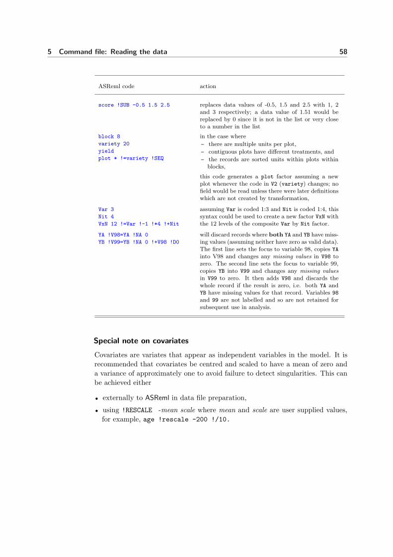
5 Command file: Reading the data 58

ASReml code action

score !SUB -0.5 1.5 2.5 replaces data values of -0.5, 1.5 and 2.5 with 1, 2and 3 respectively; a data value of 1.51 would bereplaced by 0 since it is not in the list or very closeto a number in the list

block 8

variety 20

yield

plot * !=variety !SEQ

in the case where

– there are multiple units per plot,

– contiguous plots have different treatments, and

– the records are sorted units within plots withinblocks,

this code generates a plot factor assuming a newplot whenever the code in V2 (variety) changes; nofield would be read unless there were later definitionswhich are not created by transformation,

Var 3

Nit 4

VxN 12 !=Var !-1 !*4 !+Nit

assuming Var is coded 1:3 and Nit is coded 1:4, thissyntax could be used to create a new factor VxN withthe 12 levels of the composite Var by Nit factor.

YA !V98=YA !NA 0

YB !V99=YB !NA 0 !+V98 !D0

will discard records where both YA and YB have miss-ing values (assuming neither have zero as valid data).The first line sets the focus to variable 98, copies YA

into V98 and changes any missing values in V98 tozero. The second line sets the focus to variable 99,copies YB into V99 and changes any missing valuesin V99 to zero. It then adds V98 and discards thewhole record if the result is zero, i.e. both YA andYB have missing values for that record. Variables 98

and 99 are not labelled and so are not retained forsubsequent use in analysis.

Special note on covariates

Covariates are variates that appear as independent variables in the model. It isrecommended that covariates be centred and scaled to have a mean of zero anda variance of approximately one to avoid failure to detect singularities. This canbe achieved either

• externally to ASReml in data file preparation,

• using !RESCALE -mean scale where mean and scale are user supplied values,for example, age !rescale -200 !/10.

5 Command file: Reading the data 59

5.6 Datafile line

The purpose of the datafile line is to

• nominate the data file,

• specify qualifiers to modify

– the reading of the data,– the output produced,– the operation of ASReml.

NIN Alliance Trial 1989

variety !A...

row 22

column 11

nin89aug.asd !skip 1

yield ∼ mu variety...

Data line syntax

The datafile line appears in the ASReml command file in the form

datafile [qualifiers]

• datafile is the path name of the file that contains the variates, factors, covari-ates, traits (response variates) and weight variables represented as data fields,see Chapter 4; enclose the path name in quotes if it contains embedded blanks,

• the qualifiers tell ASReml to modify either

– the reading of the data and/or the output produced, see Table 5.2 below fora list of data file related qualifiers,

– the operation of ASReml, see Tables 5.3 to 5.6 for a list of job control qual-ifiers

• the data file related qualifiers must appear on the data file line,

• the job control qualifiers may appear on the data file line or on following lines,

• the arguments to qualifiers are represented by the following symbols

f — a filename,n — an integer number, typically a count,p — a vector of real numbers, typically in increasing order,r — a real number,s — a character string,t — a model term label,v — the number or label of a data variable,vlist — a list of variable labels.

5 Command file: Reading the data 60

5.7 Data file qualifiers

Table 5.2 lists the qualifiers relating to data input. Use the Index to check forexamples or further discussion of these qualifiers.

Table 5.2: Qualifiers relating to data input and output

qualifier action

Frequently used data file qualifier

!SKIP n causes the first n records of the (non-binary) data file to beignored. Typically these lines contain column headings forthe data fields.

Other data file qualifiers

!CSV used to make consecutive commas imply a missing value; thisis automatically set if the file name ends with .csv or .CSV

(see Section 4.2)

,

!FILTER v !SELECT n enables a subset of the data to be analysed; v is the numberor name of a data field. When reading data, the value infield v is checked after any transformations are performed. If!select is omitted, records with zero in field v are omittedfrom the analysis. Otherwise, records with n in field v areretained and all other records are omitted. Warning If thefilter column contains a missing value, the value from theprevious non-missing record is assumed in that position.

!FORMAT s supplies a Fortran like FORMAT statement for reading fixed for-mat files. A simple example is !FORMAT(3I4,5F6.2) whichreads 3 integer fields and 5 floating point fields from the first42 characters of each data line. A format statement is en-closed in parentheses and may include 1 level of nested paren-theses, for example, e.g. !FORMAT(4x,3(I4,f8.2)). Fielddescriptors are

• rX to skip r character positions,

• rAw to define r consecutive fields of w characters width,

• rIw to define r consecutive fields of w characters width,and

• rFw.d to define r consecutive fields of w characters width;d indicates where to insert the decimal point if it is notexplicitly present in the field,

where r is an optional repeat count.

In ASReml, the A and I field descriptors are treated identi-cally and simply set the field width. Whether the field isinterpreted alphabetically or as a number is controlled by the!A qualifier.

5 Command file: Reading the data 61

Qualifiers relating to data input and output

qualifier action

Other legal components of a format statement are

• the , character; required to separate fields - blanks arenot permitted in the format.

• the / character; indicates the next field is to be read fromthe next line. However a / on the end of a format to skipa line is not honoured.

• BZ; the default action is to read blank fields as missingvalues. * and NA are also honoured as missing values. Ifyou wish to read blank fields as zeros, include the stringBZ.

• the string BM; switches back to ’blank missing’ mode.

• the string Tc; moves the ’last character read’ pointer to lineposition c so that the next field starts at position c + 1.For example T0 goes back to the beginning of the line.

• the string D; invokes debug mode.

A format showing these components is!FORMAT(D,3I4,8X,A6,3(2x,F5.2)/4x,BZ,20I1) and issuitable for reading 27 fields from 2 data records such as111122223333xxxxxxxxALPHAFxx 4.12xx 5.32xx 6.32

xxxx123 567 901 345 7890

!MERGE c f [ !SKIP n ]New

[ !MATCH a b ] may be specified on a line following the datafile line.The purpose is to combine data fields from the (primary) datafile with data fields from a secondary file (f). The effect is toopen the named file (skip n lines) and then insert the columnsfrom the new file into field positions starting at position c.If !MATCH a b is specified, ASReml checks that the field a(0 < a < c) has the same value as field b. If not, it is assumedthat the merged file has some missing records and missingvalues are inserted into the data record and the line from theMERGE file is kept for comparison with the next record. Atthis stage it is expected that the lines in the MERGE fileare in the same order as the corresponding lines occur in theprimary data file, and that there are no extraneous lines inthe MERGE file. (It is proposed to extend this so the ordersdo not need to agree and that multiple lines in the primaryfile could be merged with the same line of the MERGE file.)

5 Command file: Reading the data 62

Qualifiers relating to data input and output

qualifier action

For example, assuming the field definitions define 10 fields,PRIMARY.DAT !skip 1

!MERGE 6 SECOND.DAT !SKIP 1 !MATCH 1 6

would obtain the first five fields from PRIMARY.DAT andthe next five from SECOND.DAT, checking that the first fieldin each file has the same value.Thus each input record is obtained by combining informationfrom each file, before any transformations are performed.

!READ n formally instructs ASReml to read n data fields from the datafile. It is needed when there are extra columns in the data filethat must be read but are only required for combination intoearlier fields in transformations, or when ASReml attempts toread more fields than it needs to.

!RECODE is required when reading a binary data file with pedigree iden-tifiers that have not been recoded according to the pedigreefile. It is not needed when the file was formed using the !SAVEoption but will be needed if formed in some other way (seeSection 4.2).

!RREC [n]New

causes ASReml to read n records or to read up to a datareading error if n is omitted, and then process the records ithas. This allows data to be extracted from a file which con-tains trailing non-data records (for example extracting thepredicted values from a .pvs file). The argument (n) speci-fies the number of data records to be read. If not supplied,ASReml reads until a data reading error occurs, and then pro-cesses the data it has. Without this qualifier, ASReml abortsthe job when it encounters a data error. See !RSKIP.

!RSKIP n [s]New

allows ASReml to skip lines at the heading of a file down to(and including) the nth instance of string s. For example, toread back the third set predicted values in a .pvs file, youwould specify

!RREC !RSKIP 4 ’ Ecode’

since the line containing the 4th instance of ’ Ecode’ imme-diately precedes the predicted values. The !RREC qualifiermeans that ASReml will read until the end of the predict ta-ble. The keyword Ecode which occurs once at the beginningand then immediately before each block of data in the .pvs

file is used to count the sections.

5 Command file: Reading the data 63

Combining rows from separate files

ASReml can read data from multiple files provided the files have the same layout.New

The file specified as the ’primary data file’ in the command file can contain linesof the form!INCLUDE <filename> !SKIP n

where <filename> is the (path)name of the data subfile and !SKIP n is anoptional qualifier indicating that the first n lines of the subfile are to be skipped.After reading each subfile, input reverts to the primary data file.

Typically, the primary data file will just contain !INCLUDE statements identifyingthe subfiles to include. For example, you may have data from a series of relatedexperiments in separate data files for individual analysis. The primary data filefor the subsequent combined analysis would then just contain a set of !INCLUDEstatements to specify which experiments were being combined.

If the subfiles have CSV format, they should all have it and the !CSV file should bedeclared on the primary datafile line. This option is not available in combinationwith !MERGE.

5.8 Job control qualifiers

The following tables list the job control qualifiers. These change or control variousaspects of the analysis. Job control qualifiers may be placed on the datafile lineand following lines. They may also be defined using an environment variablecalled ASREML QUAL. The environment variable is processed immediately after thedatafile line is processed. All qualifier settings are reported in the .asr file. Usethe Index to check for examples or further discussion of these qualifiers.

Important Many of these are only required in very special circumstances andnew users should not attempt to understand all of them. You do need to under-stand that all general qualifiers are specified here. Many of these qualifiers arereferenced in other chapters where their purpose will be more evident.

5 Command file: Reading the data 64

Table 5.3: List of commonly used job control qualifiers

qualifier action

!CONTINUE is used to restart/resume iterations from the point reached ina previous run. This qualifier can alternately be set from thecommand line using the option letters C (continue) or F (fi-nal) (see Section 12.3 on command line options). After eachiteration, ASReml writes the current values of the variance pa-rameters to a file with extension .rsv (re-start values) withinformation to identify individual variance parameters. The!CONTINUE qualifier causes ASReml to scan the .rsv file forparameter values related to the current model replacing thevalues obtained from the .as file before iteration resumes.If the model has changed, ASReml will pick up the values itrecognises as being for the same terms. Furthermore, AS-Reml will use estimates in the .rsv file for certain models toprovide starting values for certain more general models, in-serting reasonable defaults where necessary. The transitionsrecognised are listed and discussed in Section 7.10.

DIAG to FA1

DIAG to CORUH (uniform heterogeneous)CORUH to FA1

FAi to FAi+1FAi to CORGH (full heterogeneous)FAi to US (full heterogeneous)CORGH (heterogeneous) to US

!CONTRAST s t pNew

provides a convenient way to define contrasts among treat-ment levels. !CONTRAST lines occur as separate lines betweenthe datafile line and the model line.

s is the name of the model term being defined.t is the name of an existing factor.p is the list of contrast coefficients. For example

!CONTRAST LinN Nitrogen 3 1 -1 -3

defines LinN as a contrast based on the 4 (implied by thelength of the list) levels of factor Nitrogen. Missing values inthe factor become missing values in the contrast. Zero valuesin the factor (no level assigned) become zeros in the contrast.The user should check that the levels of the factor are in theorder assumed by contrast (check the .ass or .sln or .tab

files). It may also be used on the implicit factor Trait ina multivariate analysis provided it implicitly identifies thenumber of levels of Trait; the number of traits is implied bythe length of the list. Thus, if the analysis involves 5 traits,

!CONTRAST Time Trait 1 3 5 10 20

5 Command file: Reading the data 65

List of commonly used job control qualifiers

qualifier action

!FCON

Newadds a ’conditional’ F-statistic column to the Analysis of Vari-ance table. It enables inference for fixed effects in the densepart of the linear mixed model to be conducted so as to re-spect both structural and intrinsic marginality (see Section2.6). The detail of exactly which terms are conditioned on isreported in the .aov file. The principle used in determiningthis conditional test is that a term cannot be adjusted foranother term which encompasses it explicitly (e.g. term A.C

cannot be adjusted for A.B.C) or implicitly (e.g. term REGION

cannot be adjusted for LOCATION when locations are actuallynested in regions although they are coded independently).

!MAXIT n sets the maximum number of iterations; the default is 10.ASReml iterates for n iterations unless convergence is achievedfirst. Convergence is presumed when the REML log-likelihoodchanges less than 0.002* current iteration number and theindividual variance parameter estimates change less than 1%.

If the job has not converged in n iterations, use the !CONTINUEqualifier to resume iterating from the current point.

To abort the job at the end of the current iteration, create afile named ABORTASR.NOW in the directory in which the job isrunning. At the end of each iteration, ASReml checks for thisfile and if present, stops the job, producing the usual outputbut not producing predicted values since these are calculatedin the last iteration. Creating FINALASR.NOW will stop ASRemlafter one more iteration (during which predictions will beformed).

On case sensitive operating systems (eg. Unix), the filename(ABORTASR.NOW or FINALASR.NOW) must be upper case. Notethat the ABORTASR.NOW file is deleted so nothing of importanceshould be in it. If you perform a system level abort (CTRL Cor close the program window) output files other than the .rsvfile will be incomplete. The .rsv file should still be functionalfor resuming iteration at the most recent parameter estimates(see !CONTINUE).

Use !MAXIT 1 where you want estimates of fixed effects andpredictions of random effects for the particular set of varianceparameters supplied as initial values. Otherwise the estimatesand predictions will be for the updated variance parameters(see the !BLUP qualifier below).

5 Command file: Reading the data 66

List of commonly used job control qualifiers

qualifier action

If !MAXIT 1 is used and an Unstructured Variance model is fit-ted, ASReml will perform a Score test of the US matrix. Thus,assume the variance structure is modelled with reduced pa-rameters, if that modelled structure is then processed as theinitial values of a US structure, ASReml tests the adequacyof the reduced parameterization.

!SUM

Newcauses ASReml to report a general description of the distribu-tion of the data variables and factors and simple correlationsamong the variables for those records included in the anal-ysis. This summary will ignore data records for which thevariable being analysed is missing unless a multivariate anal-ysis is requested or missing values are being estimated. Theinformation is written to the .ass file.

!X v !Y v !G v !JOIN is used to plot the (transformed) data. Use !X to specifythe x variable, !Y to specify the y variable and !G to specifya grouping variable. !JOIN joins the points when the xvalue increases between consecutive records. The groupingvariable may be omitted for a simple scatter plot. Omit !Y

y produce a histogram of the x variable.

For example,!X age !Y height !G sex

Note that the graphs are only produced in the graphics ver-sions of ASReml (Section 12.3).

For multivariate repeated measures data, ASReml can plotthe response profiles if the first response is nominated withthe !Y qualifier and the following analysis is of the multi-variate data. ASReml assumes the response variables are incontiguous fields and are equally spaced. For exampleResponse profiles

Treatment !A

Y1 Y2 Y3 Y4 Y5

rat.asd !Y Y1 !G Treatment !JOIN

Y1 Y2 Y3 Y4 Y5 ∼ Trait Treatment Trait.Treatment

5 Command file: Reading the data 67

Table 5.4: List of occasionally used job control qualifiers

qualifier action

!ASMV n indicates a multivariate analysis is required although the datais presented in a univariate form. ’Multivariate Analysis’ isused in the narrow sense where an unstructured error variancematrix is fitted across traits, records are independent, andobservations may be missing for particular traits, see Chapter8 for a complete discussion.

The data is presumed arranged in lots of n records where n isthe number of traits. It may be necessary to expand the datafile to achieve this structure, inserting a missing value NA onthe additional records. This option is sometimes relevant forsome forms of repeated measures analysis. There will need tobe a factor in the data to code for trait as the intrinsic Trait

factor is undefined when the data is presented in a univariatemanner.

!ASUV indicates that a univariate analysis is required although thedata is presented in a multivariate form. Specifically, it allowsyou to have an error variance other than I ⊗ Σ where Σ isthe unstructured (US, see Table 7.3) variance structure. Ifthere are missing values in the data, include !f mv on theend of the linear model. It is often also necessary to specifythe !S2==1 qualifier on the R-structure lines. The intrinsicfactor Trait is defined and may be used in the model. SeeChapter 8 for more information.

This option is used for repeated measures analysis when thevariance structure required is not the standard multivariateunstructured matrix.

!COLFAC v is used with !SECTION v and !ROWFAC v to instruct ASReml toset up R structures for analysing a multi-environment trialwith a separable first order autoregressive model for each site(environment). v is the name of a factor or variate containingcolumn numbers (1 . . . nc where nc is the number of columns)on which the data is to be sorted. See !SECTION for moredetail.

5 Command file: Reading the data 68

List of occasionally used job control qualifiers

qualifier action

!DDF [i]New

requests computation of the approximate denominatordegrees of freedom according to Kenward and Roger (1997)for the Analysis of Variance of fixed effects terms in the densepart of the linear mixed model. There are three options fori: i = −1 suppresses computation, i = 1 and i = 2 computethe denominator d.f. using numerical and algebraic methodsrespectively.If i is omitted then i = 2 is assumed.If !DDF i is omitted, i = −1 is assumed except for small jobs(< 10 parameters, < 500 fixed effects, < 10, 000 equationsand < 100 Mbyte workspace) when i = 2.

Calculation of the denominator degrees of freedom is compu-tationally expensive. Numerical derivatives require an extraevaluation of the mixed model equations for every varianceparameter. Algebraic derivatives require a large dense ma-trix, potentially of order number of equations plus number ofrecords and is not available when MAXIT is 1 or for multivari-ate analysis.

!DISPLAY n is used to select particular graphic displays. In spatial anal-ysis of field trials, four graphic displays are possible (see Sec-tion 13.4). Coding these

1=variogram2=histogram4=row and column trends8=perspective plot of residuals,

set n to the sum of the codes for the desired graphics. Thedefault is 9. These graphics are only displayed in versionsof ASReml linked with Winteracter (that is, Linux, Sun andPC) versions. Line printer versions of these graphics are writ-ten to the .res file. See the G command line option (Section12.3 on graphics) for how to save the graphs in a file for print-ing.Use !NODISPLAY to suppress graphic displays.

!EPS sets hardcopy graphics file type to .eps.

!G v is used to set a grouping variable for plotting, see !X.

5 Command file: Reading the data 69

List of occasionally used job control qualifiers

qualifier action

!GKRIGE [p]New

controls the expansion of !PVAL lists for fac(X,Y ) modelterms. For kriging prediction in 2 dimensions (X,Y ), theuser will typically want to predict at a grid of values, notnecessarily just at data combinations. The values at whichthe prediction is required can be specified separately for Xand Y using two !PVAL statements. Normally, predict pointswill be defined for all combinations of X and Y values. Thisqualifier is required (with optional argument 1) to specify thelists are to be taken in parallel. The lists must be the samelength if to be taken in parallel.Be aware that adding two dimensional prediction points islikely to substantially slow iterations because the variancestructure is dense and becomes larger. For this reason, AS-Reml will ignore the extra PVAL points unless either !FINALor !GKRIGE are set, to save processing time.

!HPGL [2] sets hardcopy graphics file type to HP GL. An argument of2 sets the hardcopy graphics file type to HP GL 2

!JOIN is used to join lines in plots, see !X.

!MBF mbf(v,n) fNew

[!SKIP k ] specified on a separate line after the datafile line predefinesthe model term mbf(v,n) as a set of n covariates indexedby the data values in variable v. MBF stands for My BasisFunction and uses the same mechanism as the leg(), pol()

and spl() model functions but with covariates supplied bythe user. The file f should contain 1+n fields where the firstfield contains the values which are in the data variable or atwhich prediction is required, and the remaining n fields definethe corresponding covariate values. !SKIP k is an optionalqualifier which requests the first k lines of the file be ignored.

!MVINCLUDE When missing values occur in the design ASRemlwill reportthis fact and abort the job unless !MVINCLUDE is specified (seeSection 6.10); then missing values are treated as zeros. Usethe !D transformation to drop the records with the missingvalues.

!MVREMOVE instructs ASReml to discard records which have missing valuesin the design matrix (see Section 6.10).

!NODISPLAY suppresses the graphic display of the variogram and residualswhich is otherwise produced for spatial analyses in the PC andSUN versions. This option is usually set on the command lineusing the option letter N (see Section 12.3 on graphics). Thetext version of the graphics is still written to the .res file.

!PS sets hardcopy graphics file type to .ps.

5 Command file: Reading the data 70

List of occasionally used job control qualifiers

qualifier action

!PVAL v p is a mechanism for specifying the particular points to bepredicted for covariates modelled using fac(v), leg(v,k),spl(v,k) and pol(v,k). The points are specified here sothat they can be included in the appropriate design matrices.v is the name of a data field. p is the list of values at whichprediction is required. See !GKRIGE for special conditions per-taining to fac(x,y) prediction.

!PVAL f vlist is used to read predict points for several variables from a filef. vlist is the names of the variables having values defined. Ifthe file contains unwanted fields, put the pseudo variate labelskip in the appropriate position in vlist to ignore them. Thefile should only have numeric values. predict points cannotbe specified for design factors.

!ROWFAC v is used with !SECTION v and !COLFAC v to instruct ASReml tosetup the R structures for multi-environment spatial analysis.v is the name of a factor or variate containing row numbers(1 . . . nr where nr is the number of rows) on which the datais to be sorted. See !SECTION for more detail.

!SECTION v specifies the factor in the data that defines the data sections.This qualifier enables ASReml to check that sections havebeen correctly dimensioned but does not cause ASReml tosort the data unless !ROWFAC and !COLFAC are also specified.Data is assumed to be presorted by section but will be sortedon row and column within section. The following is a basicexample assuming 5 sites (sections).

When !ROWFAC v and !COLFAC v are both specified ASRemlgenerates the R structures for a standard AR ⊗ AR spatialanalysis. The R structure lines that a user would normallybe required to work out and type into the .as file (see theexample of Section 15.6) are written to the .res file. Theuser may then cut and paste them into the .as file for a laterrun if the structures need to be modified.

Basic multi-environment trial analysis

site 5 # sites coded 1 ... 5

column * # columns coded 1 ...

row * # rows coded 1 ...

variety !A # variety names

yield

met.dat !SECTION site !ROWFAC row !COLFAC col

yield ∼ site !r variety site.variety !f mv

site 2 0 # variance header line

# asreml inserts the 10 lines required to define

# the R structure lines for the five sites here

5 Command file: Reading the data 71

List of occasionally used job control qualifiers

qualifier action

!SPLINE spl(v,n) p defines a spline model term with an explicit set of knot points.The basic form of the spline model term, spl(v), is definedin Table 6.1 where v is the underlying variate. The basic formuses the unique data values as the knot points. The extendedform is spl(v,n) which uses n knot points. Use this !SPLINEqualifier to supply an explicit set of n knot points (p) for themodel term t. Using the extended form without using thisqualifier results in n equally spaced knot points being used.The !SPLINE qualifier may only be used on a line by itselfafter the datafile line and before the model line.

When knot points are explicitly supplied they should be inincreasing order and adequately cover the range of the dataor ASReml will modify them before they are applied. If youchoose to spread them over several lines use a comma at theend of incomplete lines so that ASReml will to continue read-ing values from the next line of input. If the explicit points donot adequately cover the range, a message is printed and thevalues are rescaled unless !NOCHECK is also specified. Inade-quate coverage is when the explicit range does not cover themidpoint of the actual range. See !KNOTS, !PVAL and !SCALE.

!STEP r reduces the update step sizes of the variance parameters. Thedefault value is the reciprocal of the square root of !MAXIT. Itmay be set between 0.01 and 1.0. The step size is increasedtowards 1 each iteration. Starting at 0.1, the sequence wouldbe 0.1, 0.32, 0.56, 1. This option is useful when you do nothave good starting values, especially in multivariate analyses.

!SUBSET t v pNew

forms a new factor (t) derived from an existing factor (v)by selecting a subset (p) of its levels. Missing values aretransmitted as missing and records whose level is zero aretransmitted as zero. The qualifier occupies its own line afterthe datafile line but before the linear model. e.g.

!SUBSET EnvC Env 3 5 8 9 :15 21 33

defines a reduced form of the factor Env just selecting theenvironments listed. It might then be used in the model inan interaction.

The intention is to simplify the model specification in MET(Multi Environment Trials) analyses where say Column ef-fects are to be fitted to a subset of environments. It mayalso be used on the intrinsic factor Trait in a multivariateanalysis provided it correctly identifies the number of levels ofTrait either by including the last trait number, or appendingsufficient zeros. Thus, if the analysis involves 5 traits,

!SUBSET Trewe Trait 1 3 4 0 0

5 Command file: Reading the data 72

Table 5.5: List of rarely used job control qualifiers

qualifier action

!AISINGULARITIES

Newcan be specified to force a job to continue even though a singu-larity was detected in the Average Information (AI) matrix.The AI matrix is used to give updates to the variance pa-rameter estimates. In release 1, if singularities were presentin the AI matrix, a generalized inverse was used which effec-tively conditioned on whichever parameters were identified assingular. ASReml now aborts processing if such singularitiesappear unless the !AISINGULARITIES qualifier is set. Whichparticular parameter is singular is reported in the variancecomponent table printed in the .asr file.

The most common reason for singularities is that the userhas overspecified the model and is likely to misinterpret theresults if not fully aware of the situation. Overspecificationwill occur in a direct product of two unconstrained variancematrices (see Section 2.4), when a random term is confoundedwith a fixed term and when there is no information in the dataon a particular component.

The best solution is to reform the variance model so thatthe ambiguity is removed, or to fix one of the parameters inthe variance model so that the model can be fitted. For in-stance, if !ASUV is specified, you may also need !S2==1. Onlyrarely will it be reasonable to specify the !AISINGULARITIES

qualifier.

!BMP sets hardcopy graphics file type to .bmp.

!BRIEF [n]New

suppresses some of the information written to the .asr file.The data summary and regression coefficient estimates aresuppressed. This qualifier should not be used for initial runsof a job until the user has confirmed from the data summarythat the data is correctly interpreted by ASReml . Use !BRIEF2 to cause the predicted values to be written to the .asr fileinstead of the .pvs file. Use !BRIEF -1 to get BLUE (fixedeffect) estimates reported in .asr file. The !BRIEF qualifiermay be set with the B command line option.

!BLUP n restricts ASReml to performing only part of the first iteration.The estimation routine is aborted aftern = 1: forming the estimates of the vector of fixed and ran-dom effects,n = 2: forming the estimates of the vector of fixed and ran-dom effects, REML log-likelihood and residuals (this is thedefault),n = 3: forming the estimates of the vector of fixed and ran-dom effects, REML log-likelihood, residuals and inverse coef-ficient matrix.

5 Command file: Reading the data 73

List of rarely used job control qualifiers

qualifier action

ASReml prints its standard reports as if it had completed theiteration normally, but since it has not completed it, someof the information printed will be incorrect. In particular,variance information on the variance parameters will alwaysbe wrong. Standard errors on the estimates will be wrongunless n=3. Residuals are not available if n=1. Use of n=3or n=2 will halve the processing time when compared to thealternative of using !MAXIT 1. However, !MAXIT 1 does resultin a complete and correct output report.

!DATAFILE f specifies the datafile name replacing the one obtained fromthe datafile line. It is required when different !PATHS (see!DOPATH in Table 12.3) of a job must read different files. The!SKIP qualifier, if specified, will be applied when reading thefile.

!DENSE n sets the number of equations solved densely up to a maximumof 5000. By default, sparse matrix methods are applied to therandom effects and any fixed effects listed after random fac-tors or whose equation numbers exceed 800. Use !DENSE n toapply sparse methods to effects listed before the !r (reduc-ing the size of the DENSE block) or if you have large fixedmodel terms and want them included in the ANOVA table.Individual model terms will not be split so that only part isin the dense section. n should be kept small (<100) for fasterprocessing.

!DF n alters the error degrees of freedom from ν to ν + n. Thisqualifier might be used when analysing pre-adjusted data toreduce the degrees of freedom (n negative) or when weightsare used in lieu of actual data records to supply error infor-mation (n positive). The degrees of freedom is only used inthe calculation of the residual variance in a univariate singlesite analysis. The option will have no effect in analyses withmultiple error variances (for sites or traits) other than in thereported degrees of freedom. Use !ADJUST r rather than !DF

n if r is not a whole number. Use with !YSS r to supplyvariance when data fully fitted.

5 Command file: Reading the data 74

List of rarely used job control qualifiers

qualifier action

!EMFLAG n

New !PXEM nCaution

requests ASReml use Expectation-Maximization (EM) ratherthan Average Information (AI) updates when the AI updateswould make a US structure non-positive definite. This onlyapplies to US structures and is still under development. When!GP is associated with a US structure, ASReml checks whetherthe updated matrix is positive definite (PD). If not, it re-places the AI update with an EM update. If the non PDcharacteristic is transitory, then the EM update is only usedas necessary. If the converged solution would be non PD,there will be a EM update each iteration even though !EM isomitted.EM is notoriously slow at finding the solution and ASRemlincludes several modified schemes, discussed by Cullis et al.(2004), particularly relevant when the AI update is consis-tently outside the parameter space. These include optionallyperforming extra local EM or PXEM (Parameter ExtendedEM) iterates. These can dramatically reduce the number ofiterates required to find a solution near the boundary of theparameter space but do not always work well when there areseveral matrices on the boundary. The options are

!EMFLAG [1] Standard EM plus 10 local EM steps!EMFLAG 2 Standard EM plus 10 local PXEM steps!PXEM [2] Standard EM plus 10 local PXEM steps!EMFLAG 3 Standard EM plus 10 local EM steps!EMFLAG 4 Standard EM plus 10 local EM steps!EMFLAG 5 Standard EM only!EMFLAG 6 Single local PXEM!EMFLAG 7 Standard EM plus 1 local EM step!EMFLAG 8 Standard EM plus 10 local EM steps

Options 3 and 4 cause all US structures to be updated by(PX)EM if any particular one requires EM updates.The test of whether the AI updated matrix is positive defini-tite is based on absorbing the matrix to check all pivots arepositive. Repeated EM updates may bring the matrix closerto being singular. This is assessed by dividing the pivot ofthe first element with the first diagonal element of the ma-trix. If it is less than 10−7 (this value is consistent withthe multiple partial correlation of the first variable with therest being greater than 0.9999999, ASReml fixes the matrixat that point and estimates any other parameters conditionalon these values. To preceed with further iterations withoutfixing the matrix values would ultimately make the matrixsuch that it would be judged singular resulting the analysisbeing aborted.

5 Command file: Reading the data 75

List of rarely used job control qualifiers

qualifier action

!EQORDER oNew

modifies the algorithm used for choosing the order for solv-ing the mixed model equations. A new algorithm devisedfor release 2 is now the default and is formally selected by!EQORDER 3. The algorithm used for release 1 is essentiallythat selected by !EQORDER 1. The new order is generally su-perior. !EQORDER -1 instructs ASReml to process the equa-tions in the order they are specified in the model. Generallythis will make a job much slower, if it can run at all. It isuseful if the model has a suitable order as in the IBD model

Y ∼ mu !r ! giv(id) id !giv(id) invokes a dense inverse of an IBD matrix and id

has a sparse structured inverse of an additive relationshipmatrix. While !EQORDER 3 generates a more sparse solution,!EQORDER -1 runs faster.

!EXTRA n forces another mod(n,10) rounds of iteration after apparentconvergence. The default for n is 1. This qualifier has lowerpriority than !MAXIT and ABORTASR.NOW (see !MAXIT for de-tails).Convergence is judged by changes in the REML log-likelihoodvalue and variance parameters. However, sometimes the vari-ance parameter convergence criteria has not been satisfied.

!LAST <factor1 > <lev1 >NewDifficult

[<fac2 > <lev2 > <fac3 > <lev3 >]limits the order in which equations are solved in ASReml byforcing equations in the sparse partition involving the first<levi > equations of <factori > to be solved after all otherequations in the sparse partition. Is intended for use whenthere are multiple fixed terms in the sparse equations so thatASReml will be consistent in which effects are identified assingular. The test example had

!r Anim Litter !f HYS

where genetic groups were included in the definition of Anim.

Consequently, there were 5 singularities in Anim. The defaultreordering allows those singularities to appear anywhere inthe Anim and HYS terms. Since 29 genetic groups were definedin Anim, !LAST Anim 29 forces the genetic group equations tobe absorbed last (and therefore incorporate any singularities).In the more general model fitting

!r Tr.Anim Tr.Lit !f Tr.HYS

without !LAST, the location of singularities will almost surelychange if the G structures for Tr.Anim or Tr.Lit are changed,invalidating Likelihood Ratio tests between the models.

!OWN f supplies the name of a program supplied by the user in asso-ciation with the OWN variance model (page 131).

5 Command file: Reading the data 76

List of rarely used job control qualifiers

qualifier action

!PRINT n causes ASReml to print the transformed data file to base-name.asp. Ifn < 0, data fields 1...mod(n) are written to the file,n = 0, nothing is written,n = 1, all data fields are written to the file if it does not exist,n = 2, all data fields are written to the file overwriting anyprevious contents,n > 2, data fields n. . . t are written to the file where t is thelast defined column.

!PVSFORM nNew

modifies the format of the tables in the .pvs file and changesthe file extension of the file to reflect the format.!PVSFORM 1 is TAB separated: .pvs → pvs.txt

!PVSFORM 2 is COMMA separated: .pvs → pvs.csv

!PVSFORM 3 is Ampersand separated: .pvs → pvs.tex

See !TXTFORM for more detail.

!RESIDUALS [2] instructs ASReml to write the transformed data and the resid-uals to a binary file. The residual is the last field. The filebasename.srs is written in single precision unless the argu-ment is 2 in which case basename.drs is written in doubleprecision.

The file will not be written from a spatial analysis (two-dimensional error) when the data records have been sortedinto field order because the residuals are not in the sameorder that the data is stored. The residual from a spatialanalysis will have the units part added to it when units isalso fitted. The .drs file could be renamed (with extension.dbl) and used for input in a subsequent run.

!SAVE n instructs ASReml to write the data to a binary file. The fileasrdata.bin is written in single precision if the argument nis 1 or 3; asrdata.dbl is written in double precision if theargument n is 2 or 4; the data values are written before trans-formation if the argument is 1 or 2 and after transformationif the argument is 3 or 4. The default is single precision aftertransformation (see Section 4.2).

5 Command file: Reading the data 77

List of rarely used job control qualifiers

qualifier action

!SCREEN [n] [ !SMX m ]New

performs a ’Regression Screen’, a form of all subsets regres-sion. For d model terms in the DENSE equations, thereare 2d − 1 possible submodels. Since for d > 8, 2d − 1 islarge, the submodels explored are reduced by the parametersn and m so that only models with at least n (default 1) termsbut no more than m (default 6) terms are considered. Theoutput (see page 192) is a report to the .asr file with a linefor every submodel showing the sums of squares, degrees offreedom and terms in the model. There is a limit of d = 20model terms in the screen. ASReml will not allow interac-tions to be included in the screened terms. For example, toidentify which three of my set of 12 covariates best explainmy dependent variable given the other terms in the model,specify !SCREEN 3 !SMX 3. The number of models evaluatedquickly increases with d but ASReml has an arbitrary limit of900 submodels evaluated. Use the !DENSE qualifier to controlwhich terms are screened. The screen is conditional on allother terms (those in the SPARSE equations) being present.

!SLNFORM [n]New

modifies the format of the .sln file.!SLNFORM -1 prevents the .sln file from being written.!SLNFORM 1 is TAB separated: .sln becomes sln.txt

!SLNFORM 2 is COMMA separated: .sln becomes sln.csv

!SLNFORM 3 is Ampersand separated: .sln becomes sln.tex

See !TXTFORM for more detail.

!SPATIAL

Newincreases the amount of information reported on the residualsobtained from the analysis of a two dimensional regular gridfield trial. The information is written to the .res file.

!TABFORM [n]New

controls form of the .tab file!TABFORM 1 is TAB separated: .tab becomes tab.txt

!TABFORM 2 is COMMA separated: .tab becomes tab.csv

!TABFORM 3 is Ampersand separated: .tab becomes tab.tex

See !TXTFORM for more detail.

!TXTFORM [n]New

sets the default argument for !PVSFORM, !SLNFORM, !TABFORMand !YHTFORM if these are not explicitly set. !TXTFORM (or!TXTFORM 1) replaces multiple spaces with TAB and changesthe file extension to, say, sln.txt. This makes it easier toload the solutions into Excel.!TXTFORM 2 replaces multiple spaces with COMMA andchanges the file extension to, say, sln.csv. However, sincefactor labels sometimes contain COMMAS, this form is notso convenient.

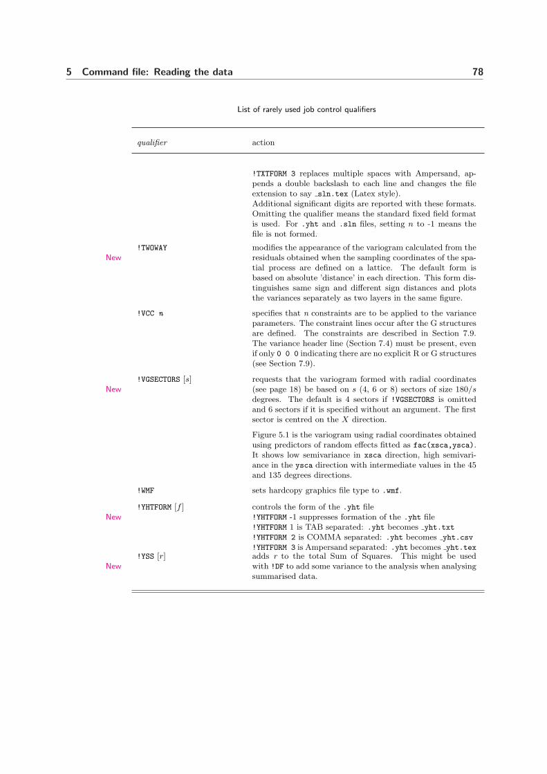
5 Command file: Reading the data 78

List of rarely used job control qualifiers

qualifier action

!TXTFORM 3 replaces multiple spaces with Ampersand, ap-pends a double backslash to each line and changes the fileextension to say sln.tex (Latex style).Additional significant digits are reported with these formats.Omitting the qualifier means the standard fixed field formatis used. For .yht and .sln files, setting n to -1 means thefile is not formed.

!TWOWAY

Newmodifies the appearance of the variogram calculated from theresiduals obtained when the sampling coordinates of the spa-tial process are defined on a lattice. The default form isbased on absolute ’distance’ in each direction. This form dis-tinguishes same sign and different sign distances and plotsthe variances separately as two layers in the same figure.

!VCC n specifies that n constraints are to be applied to the varianceparameters. The constraint lines occur after the G structuresare defined. The constraints are described in Section 7.9.The variance header line (Section 7.4) must be present, evenif only 0 0 0 indicating there are no explicit R or G structures(see Section 7.9).

!VGSECTORS [s]New

requests that the variogram formed with radial coordinates(see page 18) be based on s (4, 6 or 8) sectors of size 180/sdegrees. The default is 4 sectors if !VGSECTORS is omittedand 6 sectors if it is specified without an argument. The firstsector is centred on the X direction.

Figure 5.1 is the variogram using radial coordinates obtainedusing predictors of random effects fitted as fac(xsca,ysca).It shows low semivariance in xsca direction, high semivari-ance in the ysca direction with intermediate values in the 45and 135 degrees directions.

!WMF sets hardcopy graphics file type to .wmf.

!YHTFORM [f ]New

controls the form of the .yht file!YHTFORM -1 suppresses formation of the .yht file!YHTFORM 1 is TAB separated: .yht becomes yht.txt

!YHTFORM 2 is COMMA separated: .yht becomes yht.csv

!YHTFORM 3 is Ampersand separated: .yht becomes yht.tex!YSS [r]

Newadds r to the total Sum of Squares. This might be usedwith !DF to add some variance to the analysis when analysingsummarised data.

5 Command file: Reading the data 79

this is a test of matern

Variogram of fac(xsca,ysca) predictors21.61

2.80Distance

Semivariance

135

90

45

0

Figure 5.1 Variogram in 4 sectors for Cashmore data

Table 5.6: List of very rarely used job control qualifiers

qualifier action

!AILOADINGS iNew

controls modification to AI updates of loadings in factor an-alytic variance models. After ASReml calculates updates forvariance parameters, it checks whether the updates are rea-sonable and sometimes reduces them. For factor loadings,the default behaviour is to shrink the loadings only in thefirst iteration if they appear large. This qualifier gives someuser control. If it is specified without an argument, no (extra)shrinkage is allowed. Otherwise shrinkage is allowed in thefirst i iterations.

!CINV n prints the portion of the inverse of the coefficient matrix per-taining to the nth term in the linear model. Because themodel has not been defined when ASReml reads this line, itis up to the user to count the terms in the model to iden-tify the portion of the inverse of the coefficient matrix to beprinted. The option is ignored if the portion is not whollyin the SPARSE stored equations. The portion of the inverse isprinted to a file with extension .cii The sparse form of thematrix only is printed in the form i j Cij , that is, elementsof Cij that were not needed in the estimation process are notincluded in the file.

5 Command file: Reading the data 80

List of very rarely used job control qualifiers

qualifier action

!FACPOINTS n affects the number of distinct points recognised by the fac()

model function (Table 6.1). The default value of n is 1000 sothat points closer than 0.1% of the range are regarded as thesame point.

!KNOTS n changes the default knot points used when fitting a spline todata with more than n different values of the spline variable.When there are more than n (default 50) points, ASReml willdefault to using n equally spaced knot points.

!NOCHECK forces ASReml to use any explicitly set spline knot points (see!SPLINE) even if they do not appear to adequately cover thedata values.

!NOREORDER prevents the automatic reversal of the order of the fixed terms(in the dense equations) and possible reordering of terms inthe sparse equations.

!NOSCRATCH forces ASReml to hold the data in memory. ASReml will usu-ally hold the data on a scratch file rather than in memory. Inlarge jobs, the system area where scratch files are held maynot be large enough. A Unix system may put this file in the/tmp directory which may not have enough space to hold it.

!POLPOINTS n affects the number of distinct points recognised by the pol()

model function (Table 6.1). The default value of n is 1000 sothat points closer than 0.1% of the range are regarded as thesame point.

!PPOINTS n influences the number of points used when predicting splinesand polynomials. The design matrix generated by the leg(),pol() and spl() functions are modified to include extra rowsthat are accessed by the PREDICT directive. The default valueof n is 21 if there is no !PPOINTS qualifier. The range of thedata is divided by n-1 to give a step size i. For each point pin the list, a predict point is inserted at p + i if there is nodata value in the interval [p,p+1.1×i]. !PPOINTS is ignored if!PVAL is specified for the variable. This process also effectsthe number of levels identified by the fac() model term.

!REPORT forces ASReml to attempt to produce the standard output re-port when there is a failure of the iteration algorithm. Usu-ally no report is produced unless the algorithm has at leastproduced estimates for the fixed and random effects in themodel. Note that residuals are not included in the outputforced by this qualifier. This option is primarily intended tohelp debugging a job that is not converging properly.

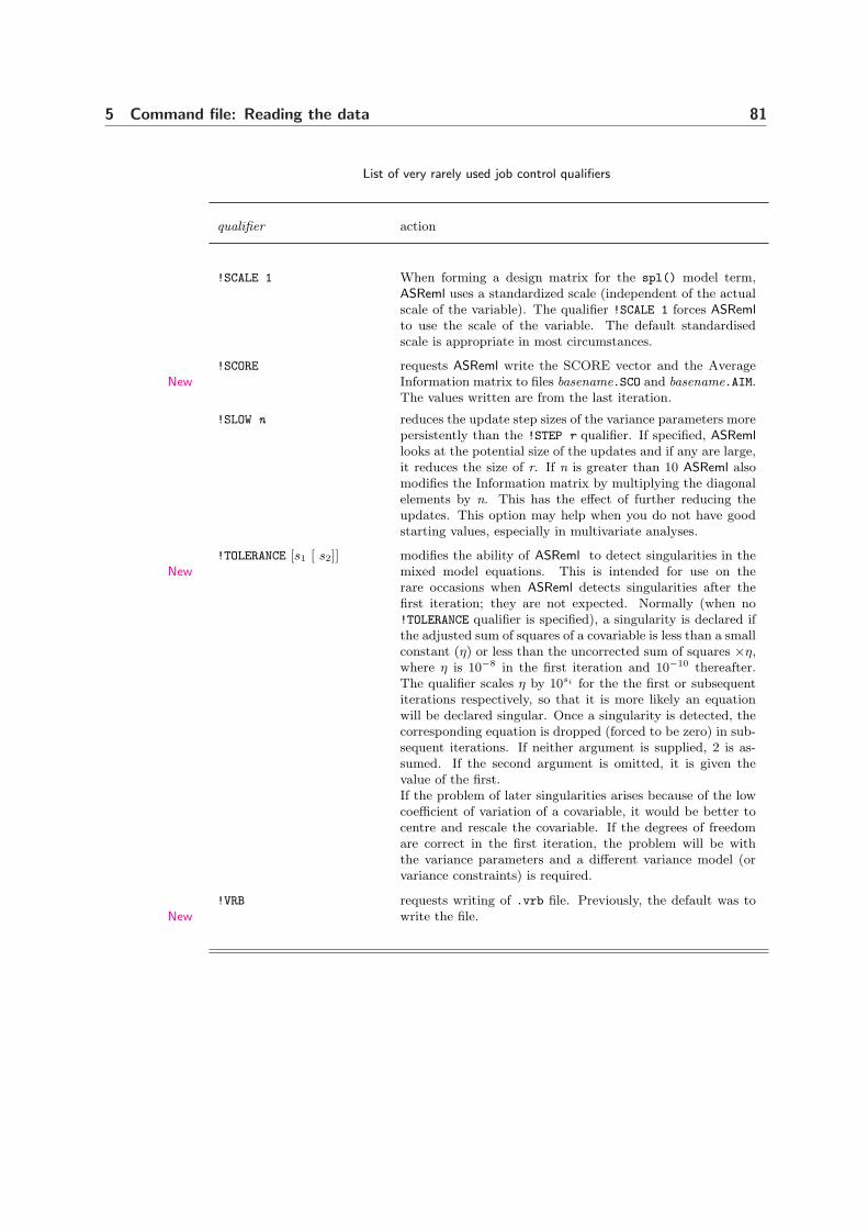
5 Command file: Reading the data 81

List of very rarely used job control qualifiers

qualifier action

!SCALE 1 When forming a design matrix for the spl() model term,ASReml uses a standardized scale (independent of the actualscale of the variable). The qualifier !SCALE 1 forces ASRemlto use the scale of the variable. The default standardisedscale is appropriate in most circumstances.

!SCORE

Newrequests ASReml write the SCORE vector and the AverageInformation matrix to files basename.SCO and basename.AIM.The values written are from the last iteration.

!SLOW n reduces the update step sizes of the variance parameters morepersistently than the !STEP r qualifier. If specified, ASRemllooks at the potential size of the updates and if any are large,it reduces the size of r. If n is greater than 10 ASReml alsomodifies the Information matrix by multiplying the diagonalelements by n. This has the effect of further reducing theupdates. This option may help when you do not have goodstarting values, especially in multivariate analyses.

!TOLERANCE [s1 [ s2]]New

modifies the ability of ASReml to detect singularities in themixed model equations. This is intended for use on therare occasions when ASReml detects singularities after thefirst iteration; they are not expected. Normally (when no!TOLERANCE qualifier is specified), a singularity is declared ifthe adjusted sum of squares of a covariable is less than a smallconstant (η) or less than the uncorrected sum of squares ×η,where η is 10−8 in the first iteration and 10−10 thereafter.The qualifier scales η by 10si for the the first or subsequentiterations respectively, so that it is more likely an equationwill be declared singular. Once a singularity is detected, thecorresponding equation is dropped (forced to be zero) in sub-sequent iterations. If neither argument is supplied, 2 is as-sumed. If the second argument is omitted, it is given thevalue of the first.If the problem of later singularities arises because of the lowcoefficient of variation of a covariable, it would be better tocentre and rescale the covariable. If the degrees of freedomare correct in the first iteration, the problem will be withthe variance parameters and a different variance model (orvariance constraints) is required.

!VRB

Newrequests writing of .vrb file. Previously, the default was towrite the file.

6 Command file: Specifying theterms in the mixed model

Introduction

Specifying model formulae in ASRemlGeneral rules

Examples

Fixed terms in the modelPrimary fixed termsSparse fixed terms

Random terms in the model

Interactions and conditional factorsInteractions

Conditional factors

Alphabetic list of model functions

Weights

Missing valuesMissing values in the response

Missing values in the explanatory variables

Some technical details about model fitting in ASRemlSparse versus dense

Ordering of terms in ASRemlAliassing and singularities

Examples of aliassing

Analysis of Variance table82

6 Command file: Specifying the terms in the mixed model 83

6.1 Introduction

The linear mixed model is specified in ASReml as a series of model terms andqualifiers. In this chapter the model formula syntax is described.

6.2 Specifying model formulae in ASReml

The linear mixed model is specified in AS-

Reml as a series of model terms and qualifiers.Model terms include factor and variate labels(Section 5.4), functions of labels, special termsand interactions of these. The model is speci-fied immediately after the datafile and any jobcontrol qualifier and/or tabulate lines. Thesyntax for specifying the model is

NIN Alliance Trial 1989

variety...

column 11

nin89.asd !skip 1

yield ∼ mu variety !r repl,

!f mv

1 2

11 column AR1 .3

22 row AR1 .3

response [!wt weight] ∼ fixed [!r random] [!f sparse fixed]

• response is the label for the response variable(s) to be analysed; multivariateanalysis is discussed in Chapter 8,

• weight is a label of a variable containing weights; weighted analysis is discussedin Section 6.7,

• ∼ separates response from the list of fixed and random terms,

• fixed represents the list of primary fixed explanatory terms, that is, variates,factors, interactions and special terms for which analysis of variance (ANOVA)type tests are required. See Table 6.1 for a brief definition of reserved modelterms, operators and commonly used functions. The full definition is in Section6.6,

• random represents the list of explanatory terms to be fitted as random effects,see Table 6.1,

• sparse fixed are additional fixed terms not included in the ANOVA table.

General rules

The following general rules apply in specifying the linear mixed model

• all elements in the model must be space separated,

• the character ∼ separates the response variables(s) from the explanatory vari-ables in the model,

6 Command file: Specifying the terms in the mixed model 84

• data fields are identified in the model by their labelsChoose labels

that will avoid

confusion– labels are case sensitive,– labels may be abbreviated (truncated) when used in the model line but care

must be taken that the truncated form is not ambiguous. If the truncatedform matches more than one label, the term associated with the first matchis assumed,

– model terms may only appear once in the model line; repeated occurrencesare ignored,

– model terms other than the original data fields are defined the first time theyappear on the model line. They may be abbreviated (truncated) if they arereferred to again provided no ambiguity is introduced.Important It is often clearer if labels are not abbreviated. If abbreviationsare used then they need to be chosen to avoid confusion.

• if the model is written over several lines, all but the final line must end with acomma to indicate that the list is continued.

In Tables 6.1 and 6.2, the arguments in model term functions are represented bythe following symbols

f — the label of a data variable defined as a model factor,

k, n — an integer number,

r — a real number,

t — a model term label (includes data variables),

v, y — the label of a data variable,

Parsing of model terms in ASReml is not very sophisticated. Where a model termtakes another model term as an argument, the argument must be predefined. Ifnecessary, include the argument in the model line with a leading ’-’ which willcause the term to be defined but not fitted. For example

Trait.male -Trait.female and(Trait.female)Also, dens is an abbeviation for density but spl(dens,7) is a different modelterm (albiet probably equivalent) to spl(density,7) because it does not repre-sent a simple truncation.

6 Command file: Specifying the terms in the mixed model 85

Table 6.1: Summary of reserved words, operators and functions

model term brief description common usage

fixed random

reserved mu the constant term or intercept√

terms mv a term to estimate missing values√

Trait multivariate counterpart to mu√

units forms a factor with a level for eachexperimental unit

√

operators . or : placed between labels to specify aninteraction

√ √

/ forms nested expansion (Section6.5)

√ √

∗ forms factorial expansion (Section6.5)

√ √

- placed before model terms to ex-clude them from the model

√ √

, placed at the end of a line to in-dicate that the model specificationcontinues on the next line

+ treated as a space√ √

! ... ! placed around some model termswhen it is important the terms notbe reordered (Section 6.4)

√

commonlyused

at(f,n) condition on level n of factor f.n may be a list of values

√ √

functions at(f) forms conditioning covariables forall levels of factor f

√ √

fac(v ) forms a factor from v with a levelfor each unique value in v

√

fac(v,y ) forms a factor with a level for eachcombination of values in v and y

√

lin(f ) forms a variable from the factorf with values equal to 1. . . n cor-responding to level(1). . . level(n) ofthe factor

√

spl(v [,k ]) forms the design matrix for the ran-dom component of a cubic spline forvariable v

√

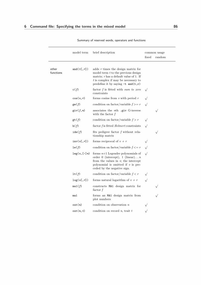
6 Command file: Specifying the terms in the mixed model 86

Summary of reserved words, operators and functions

model term brief description common usage

fixed random

otherfunctions

and(t[,r]) adds r times the design matrix formodel term t to the previous designmatrix; r has a default value of 1. Ift is complex if may be necessary topredefine it by saying -t and(t,r)

c(f) factor f is fitted with sum to zeroconstraints

√

cos(v,r) forms cosine from v with period r√

ge(f) condition on factor/variable f >= r√

giv(f,n) associates the nth .giv G-inversewith the factor f

√

gt(f) condition on factor/variable f > r√

h(f) factor f is fitted Helmert constraints√

ide(f) fits pedigree factor f without rela-tionship matrix

√

inv(v[,r]) forms reciprocal of v + r√

le(f) condition on factor/variable f <= r√

leg(v,[-]n) forms n+1 Legendre polynomials oforder 0 (intercept), 1 (linear). . . nfrom the values in v; the interceptpolynomial is omitted if v is pre-ceded by the negative sign.

√

lt(f) condition on factor/variable f < r√

log(v[,r]) forms natural logarithm of v + r√

ma1(f) constructs MA1 design matrix forfactor f

√

ma1 forms an MA1 design matrix fromplot numbers

√

out(n) condition on observation n√

out(n,t) condition on record n, trait t√

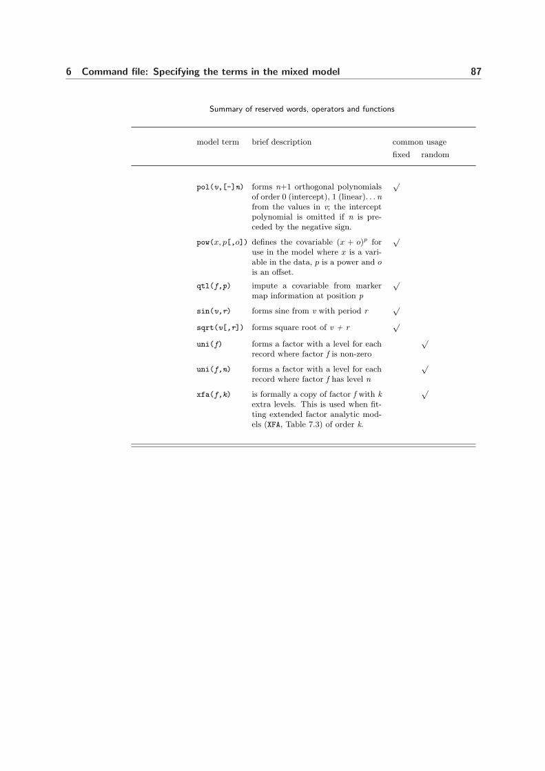
6 Command file: Specifying the terms in the mixed model 87

Summary of reserved words, operators and functions

model term brief description common usage

fixed random

pol(v,[-]n) forms n+1 orthogonal polynomialsof order 0 (intercept), 1 (linear). . . nfrom the values in v; the interceptpolynomial is omitted if n is pre-ceded by the negative sign.

√

pow(x, p[,o]) defines the covariable (x + o)p foruse in the model where x is a vari-able in the data, p is a power and ois an offset.

√

qtl(f,p) impute a covariable from markermap information at position p

√

sin(v,r) forms sine from v with period r√

sqrt(v[,r]) forms square root of v + r√

uni(f) forms a factor with a level for eachrecord where factor f is non-zero

√

uni(f,n) forms a factor with a level for eachrecord where factor f has level n

√

xfa(f,k) is formally a copy of factor f with kextra levels. This is used when fit-ting extended factor analytic mod-els (XFA, Table 7.3) of order k.

√

6 Command file: Specifying the terms in the mixed model 88

Examples

ASReml code action

yield ∼ mu variety fits a model with a constant and fixedvariety effects

yield ∼ mu variety !r block fits a model with a constant term, fixedvariety effects and random block effects

yield ∼ mu time variety time.variety fits a saturated model with fixed timeand variety main effects and time by va-riety interaction effects

livewt ∼ mu breed sex breed.sex !r sire fits a model with fixed breed, sex andbreed by sex interaction effects and ran-dom sire effects

6.3 Fixed terms in the model

Primary fixed terms

The fixed list in the model formula

• describes the fixed covariates, factors andinteractions including special functions tobe included in the ANOVA table,

• generally begins with the reserved word muwhich fits a constant term, mean or inter-cept, see Table 6.1.

NIN Alliance Trial 1989

variety...

row 22

column 11

nin89.asd !skip 1 !mvinclude

yield ∼ mu variety !r repl,

!f mv

1 2

11 column AR1 .3

22 row AR1 .3

6 Command file: Specifying the terms in the mixed model 89

Sparse fixed terms

The !f sparse fixed terms in model formula

• are the fixed covariates (for example, thefixed lin(row) covariate now included inthe model formula), factors and interac-tions including special functions and re-served words (for example mv, see Table6.1) for which ANOVA type tests are notrequired,

• include large (>100 levels) terms.

NIN Alliance Trial 1989

variety...

row 22

column 11

nin89.asd !skip 1

yield ∼ mu variety !r repl,

!f mv lin(row)

1 2

11 column AR1 .424

22 row AR1 .904

6.4 Random terms in the model

NIN Alliance Trial 1989

variety...

row 22

column 11

nin89.asd !skip 1

yield ∼ mu variety !r repl,

!f mv 1 2

11 column AR1 .424

22 row AR1 .904

The !r random terms in the model formula

• comprise random covariates, factors and in-teractions including special functions andreserved words, see Table 6.1,

• involve an initial non-zero variance compo-nent or ratio (relative to the residual vari-ance) default 0.1; the initial value can bespecified after the model term or if the vari-ance structure is not scaled identity, by syn-tax described in detail in Chapter 7,

• an initial value of its variance (ratio) may be followed by a !GP (keep positive,the default), !GU (unrestricted) or !GF (fixed) qualifier, see Table 7.4,

• use ! and ! to group model terms that may not be reordered. NormallyASReml will reorder the model terms in the sparse equations - putting smallerterms first to speed up calculations. However, the order must be preserved if theuser defines a structure for a term which also covers the following term(s) (a wayof defining a covariance structure across model terms). Grouping is specificallyrequired if the model terms are of differing sizes (number of effects). Forexample, for traits weaning weight and yearling weight, an animal modelwith maternal weaning weight should specify model terms! Trait.animal at(Trait,1).dam !when fitting a genetic covariance between the direct and maternal effects.

6 Command file: Specifying the terms in the mixed model 90

6.5 Interactions and conditional factors

Interactions

• interactions are formed by joining two or more terms with a ‘.’ or a ‘:’, forexample, a.b is the interaction of factors a and b,

• interaction levels are arranged with the levels of the second factor nested withinthe levels of the first,

• labels of factors including interactions are restricted to 31 characters of whichonly the first 20 are ever displayed. Thus for interaction terms it is oftennecessary to shorten the names of the component factors in a systematic way,for example, if Time and Treatment are defined in this order, the interactionbetween Time and Treatment could be specified in the model as Time.Treat;remember that the first match is taken so that if the label of each field beginswith a different letter, the first letter is sufficient to identify the term,

• interactions can involve model functions,

• * indicates factorial expansion (up to 5 way)a*b is expanded to a b a.ba*b*c*d is expanded to

a b c d a.b a.c a.d b.c b.d c.d a.b.c a.b.d a.c.d b.c.d a.b.c.d

• / indicates nested expansiona/b is expanded to a a.bNew

• a.(b c d) e is expanded to a.b a.c a.d e. This syntax is detected by thestring ‘.(’ and the closing parenthesis must occur on the same line and beforeany comma indicating continuation. Any number of terms may be enclosed.Each may have ‘-’ prepended to suppress it from the model. Each enclosedterm may have initial values and qualifiers following. For example,

yield∼site site.(lin(row) !r variety),at(site,1).(row .3 col .2)

expands to

yield∼site site.lin(row) !r site.variety,at(site,1).row .3 at(site,1).col .2

6 Command file: Specifying the terms in the mixed model 91

Conditional factors

A conditional factor is a factor that is present only when another factor has aparticular level.

• individual components can be specified using the at(f,n) function (see Table6.2), for example, at(site,1).row will fit row as a factor only for site 1,

• a complete set of conditional terms are specified by omitting the level spec-New

ification in the at(f) function provided the correct number of levels of f isspecified in the field definitions. Otherwise, a list of levels may be specified.

– at(f).b creates a series of model terms representing b nested within a forany model term b. A model term is created for each level of a; each hasthe size of b. For example, if site and geno are factors with 3 and 10 lev-els respectively, then for at(site).geno ASReml constructs 3 model termsat(site,1).geno at(site,2).geno at(site,3).geno, each with 10 levels,

– this is similar to forming an interaction except that a separate model term iscreated for each level of the first factor; this is useful for random terms wheneach component can have a different variance. The same effect is achievedby using an interaction (e.g. site.geno) and associating a DIAG variancestructure with the first component (see Section 7.5).

6.6 Alphabetic list of model functions

Table 6.2 presents detailed descriptions of the model functions discussed above.Note that some three letter function names may be abbreviated to the first letter.

Table 6.2: Alphabetic list of model functions and descriptions

model function action

and(t,r)

a(t,r)

overlays (adds) r times the design matrix for model term t to the existingdesign matrix. Specifically, if the model up to this point has p effects andt has a effects, the a columns of the design matrix for t are multiplied bythe scalar r (default value 1.0) and added to the last a of the p columnsalready defined. The overlaid term must agree in size with the term itoverlays. This can be used to force a correlation of 1 between two termsas in a diallel analysismale and(female)

assuming the ith male is the same individual as the ith female. Note thatif the overlaid term is complex, it must be predefined; e.g.Tr.male -Tr.female and(Tr.female).

6 Command file: Specifying the terms in the mixed model 92

Alphabetic list of model functions and descriptions

model function action

at(f,n)

@(f,n)

New at(f)

@(f)

at(f,m,n)

@(f,m,n)

defines a binary variable which is 1 if the factor f has level n for therecord. For example, to fit a row factor only for site 3, use the expressionat(site,3).row.. The string @( is equivalent to at( for this function.

at(f) is expanded to a series of terms like at(f,i) where i takes thevalues 01 to the number of levels of factor f . Since this command isinterpreted before the data is read, it is necessary to declare the numberof levels correctly in the field definition. This extended form may onlybe used as the first term in an interaction.

at(f,i,j,k) is expanded to a series of terms at(f,i) at(f,j)at(f,k). Similarly, at(f,i).X at(f,j).X at(f,k).X can be written asat(f,i,j,k).X provided at(f,i,j,k) is written as the first componentof the interaction. Any number of levels may be listed.

cos(v,r) forms cosine from v with period r. Omit r if v is radians. If v is degrees,r is 360.

con(f)

c(f)

apply sum to zero constraints to factor f. It is not appropriate for randomfactors and fixed factors with missing cells. ASReml assumes you specifythe correct number of levels for each factor. The formal effect of thecon() function is to form a model term with the highest level formallyequal to minus the sum of the preceding terms.With sum to zero constraints, a missing treatment level will generate asingularity but in the first coefficient rather than in the coefficient corre-sponding to the missing treatment. In this case, the coefficients will notbe readily interpretable. When interacting constrained factors, all cellsin the cross-tabulation should have data.

fac(v)

fac(v,y)

fac(v) forms a factor with a level for each value of x and any addi-tional points inserted as discussed with the qualifiers !PPOINTS and !PVAL.fac(v,y) forms a factor with a level for each combination of values fromv and y. The values are reported in the .res file.

giv(f,n)

g(f,n)

associates the nth .giv G-inverse with the factor. This is used whenthere is a known (except for scale) G-structure other than the additiveinverse genetic relationship matrix. The G-inverse is supplied in a filewhose name has the file extension .giv described in Section 9.6

6 Command file: Specifying the terms in the mixed model 93

Alphabetic list of model functions and descriptions

model function action

h(f)

Newh(f) requests ASReml to fit the model term for factor f usingHelmert constraints. Neither Sum-to-zero nor Helmert constraintsgenerate interpretable effects if singularities occur. ASReml runsmore efficiently if no constraints are applied. Following is an exam-ple of Helmert and sum-to-zero covariables for a factor with 5 levels.

H1 H2 H3 H4 C1 C2 C3 C4F1 -1 -1 -1 -1 1 0 0 0F2 1 -1 -1 -1 0 1 0 0F3 0 2 -1 -1 0 0 1 0F4 0 0 3 -1 0 0 0 1F5 0 0 0 4 -1 -1 -1 -1

ide(f)

i(f)

is used to take a copy of a pedigree factor f and fit it without the ge-netic relationship covariance. This facilitates fitting a second animal ef-fect. Thus, to form a direct, maternal genetic and maternal environmentmodel, the maternal environment is defined as a second animal effectcoded the same as dams. viz. !r ! animal dam ! ide(dam)

inv(v[,r]) forms the reciprocal of v + r. This may also be used to transform theresponse variable.

leg(v,[-]n) forms n+1 Legendre polynomials of order 0 (intercept), 1 (linear). . . nfrom the values in v; the intercept polynomial is omitted if n is precededby the negative sign. The actual values of the coefficients are written tothe .res file. This is similar to the pol() function described below.

lin(f)

l(f)

takes the coding of factor f as a covariate. The function is defined for fbeing a simple factor, Trait and units. The lin(f) function does notcentre or scale the variable. Motivation: Sometimes you may wish to fit acovariate as a random factor as well. If the coding is say 1. . .n, then youshould define the field as a factor in the field definition and use the lin()

function to include it as a covariate in the model. Do not centre the fieldin this case. If the covariate values are irregular, you would leave the fieldas a covariate and use the fac() function to derive a factor version.

log(v[,r]) forms the natural log of v + r. This may also be used to transform theresponse variable.

ma1

ma1(f)

creates a first-differenced (by rows) design matrix which, when defining arandom effect, is equivalent to fitting a moving average variance structurein one dimension. In the ma1 form, the first-difference operator is codedacross all data points (assuming they are in time/space order). Otherwisethe coding is based on the codes in the field indicated.

mu is used to fit the intercept/constant term. It is normally present andlisted first in the model. It should be present in the model if there are noother fixed factors or if all fixed terms are covariates or contrasts exceptin the special case of regression through the origin.

6 Command file: Specifying the terms in the mixed model 94

Alphabetic list of model functions and descriptions

model function action

mv is used to estimate missing values in the response variable. Formally thiscreates a model term with a column for each missing value. Each columncontains zeros except for a solitary -1 in the record containing the corre-sponding missing value. This is used in spatial analyses so that computingadvantages arising from a balanced spatial layout can be exploited. Theequations for mv and any terms that follow are always included in thesparse set of equations.

Missing values are handled in three possible ways during analysis (seeSection 6.10). In the simplest case, records containing missing values inthe response variable are deleted. For multivariate (including some re-peated measures) analysis, records with missing values are not deleted butASReml drops the missing observation and uses the appropriate unstruc-tured R-inverse matrix. For regular spatial analysis, we prefer to retainseparability and therefore estimate the missing value(s) by including thespecial term mv in the model.

out(n)

out(n,t)New

out(n), out(n,t) establishes a binary variable which is:out(i) 1 if data relates to observation i, (trait 1), else is 0out(i,t) 1 if data relates to observation i, (trait t), else is 0

The intention is that this be used to test/remove single observations forexample to remove the influence of an outlier or influential point. Possibleoutliers will be evident in the plot of residuals versus fitted values (seethe .res file) and the appropriate record numbers for the out() term arereported in the .res file. Note that i relates to the data analysed and willnot be the same as the record number as obtained by counting data linesin the data file if there were missing observations in the data and theyhave not been estimated. (To drop records based on the record numberin the data file, use the !D transformation in association with the !=V0

transformation.)

pol(v,n)

p(v,n)

forms a set of orthogonal polynomials of order |n| based on the uniquevalues in variate (or factor) v and any additional interpolated points,see !PPOINTS and !PVAL in Table 5.4. It includes the intercept if n ispositive, omits it if n is negative. For example, pol(time,2) forms adesign matrix with three columns of the orthogonal polynomial of degree2 from the variable time. Alternatively, pol(time,-2) is a term with twocolumns having centred and scaled linear coefficients in the first columnand centred and scaled quadratic coefficients in the second column.

The actual values of the coefficients are written to the .res file. Thisfactor could be interacted with a design factor to fit random regressionmodels. The leg() function differs from the pol() function in the waythe quadratic and higher polynomials are calculated.

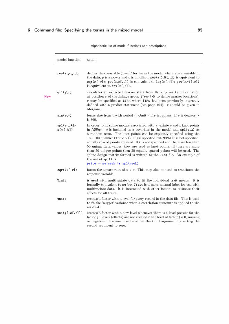
6 Command file: Specifying the terms in the mixed model 95

Alphabetic list of model functions and descriptions

model function action

pow(x, p[,o]) defines the covariable (x+o)p for use in the model where x is a variable inthe data, p is a power and o is an offset. pow(x,0.5[,o]) is equivalent tosqr(x[,o]); pow(x,0[,o]) is equivalent to log(x[,o]); pow(x,-1[,o])is equivalent to inv(x[,o]).

qtl(f,r)New

calculates an expected marker state from flanking marker informationat position r of the linkage group f(see !MM to define marker locations).r may be specified as $TPn where $TPn has been previously internallydefined with a predict statement (see page 164). r should be given inMorgans.

sin(v,r) forms sine from v with period r. Omit r if v is radians. If v is degrees, ris 360.

spl(v [,k])

s(v [,k ])

In order to fit spline models associated with a variate v and k knot pointsin ASReml, v is included as a covariate in the model and spl(v,k) asa random term. The knot points can be explicitly specified using the!SPLINE qualifier (Table 5.4). If k is specified but !SPLINE is not specified,equally spaced points are used. If k is not specified and there are less than50 unique data values, they are used as knot points. If there are morethan 50 unique points then 50 equally spaced points will be used. Thespline design matrix formed is written to the .res file. An example ofthe use of spl() isprice ∼ mu week !r spl(week)

sqrt(v[,r]) forms the square root of v + r. This may also be used to transform theresponse variable.

Trait is used with multivariate data to fit the individual trait means. It isformally equivalent to mu but Trait is a more natural label for use withmultivariate data. It is interacted with other factors to estimate theireffects for all traits.

units creates a factor with a level for every record in the data file. This is usedto fit the ’nugget’ variance when a correlation structure is applied to theresidual.

uni(f[,0[,n]]) creates a factor with a new level whenever there is a level present for thefactor f. Levels (effects) are not created if the level of factor f is 0, missingor negative. The size may be set in the third argument by setting thesecond argument to zero.

6 Command file: Specifying the terms in the mixed model 96

Alphabetic list of model functions and descriptions

model function action

uni(f,k[,n]) creates a factor with a level for every record subject to the factor levelof f equalling k, i.e. a new level is created for the factor whenever anew record is encountered whose integer truncated data value from datafield f is k. Thus uni(site,2) would be used to create an independenterror term for site 2 in a multi-environment trial and is equivalent toat(site,2).units. The default size of this model term is the number ofdata records. The user may specify a lower number as the third argument.There is little computational penalty from the default but the .sln filemay be substantially larger than needed.

xfa(f,k) Factor analytic models are discussed in Chapter 7. There are three forms,FAk, FACVk and XFAk where k is the number of factors. The XFAk form is asparse formulation that requires an extra k levels to be inserted into themixed model equations for the k factors. This is achieved by the xfa(f,k)model function which defines a design matrix based on the design matrixfor f augmented with k columns of zeros for the k factors.

6.7 Weights

Weighted analyses are achieved by using !WT weight as a qualifier to the responsevariable. An example of this is y !WT wt ∼ mu A X where y is the name of theresponse variable and wt is the name of a variate in the data containing weights.If these are relative weights (to be scaled by the units variance) then this is allthat is required. If they are absolute weights, that is, the reciprocal of knownvariances, use the !S2==1 qualifier described in Table 7.4 to fix the unit variance.When a structure is present in the residuals the weights are applied as a matrixproduct. If Σ is the structure and W is the diagonal matrix constructed from thecaution

square root of the values of the variate weight, then R−1 = WΣ−1W . Negativeweights are treated as zeros.

6.8 Generalized Linear Models

ASReml includes facilities for fitting the family of Generalized Linear Models(GLMs, McCullagh and Nelder, 1994). GLMs are specified by qualifiers after thename of the dependent variable but before the∼ character. Table 6.3 lists the link

6 Command file: Specifying the terms in the mixed model 97

function qualifiers which relate the linear predictor (η) scale to the observation(µ =E[y]) scale. Table 6.4 lists the distributions and other qualifiers.

A second dependent variable may be specified if a bivariate analysis is requiredbut it will always be treated as a normal variate (no syntax is provided forspecifying GLM attributes for it). The !ASUV qualifier is required in this situationfor the GLM weights to be utilized.

Table 6.3 Link qualifiers and functions

Qualifier Link Inverse Link Available with!IDENTITY η = µ µ = η All

!SQRT η =√

µ µ = η2 Poisson

!LOGARITHM η = ln(µ) µ = exp(η)Normal, Poisson,Negative Binomial,Gamma

!INVERSE η = 1/µ µ = 1/ηNormal, Gamma,Negative Binomial

!LOGIT η = µ/(1− µ) µ = 1(1+exp(−η)) Binomial

!PROBIT η = Φ−1(µ) µ = Φ(η) Binomial

!COMPLOGLOG η = ln(−ln(1− µ)) µ = 1− e−eηBinomial

where µ is the mean on the data scale and η = Xτ is the linear predictor on theunderlying scale.

Table 6.4: GLM qualifiers

qualifiers action

Distributions where µ is the mean on the data scale calculated from η = Xτ ,nis the count specified by the !TOTAL qualifier, v is the varianceexpression for the distribution, d is the deviance expression forthe distribution, y is the observation and φ is a parameter setwith the !PHI qualifier. The default link is listed first followed bypermitted alternatives.

!NORMAL [ !LOGARITHM | !INVERSE ]The model is fitted on the log/inverse scale but the residuals areon the natural scale.

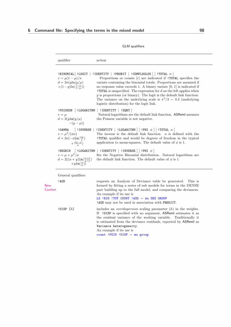
6 Command file: Specifying the terms in the mixed model 98

GLM qualifiers

qualifier action

!BINOMIAL

v = µ(1− µ)/nd = 2n(yln(y/µ)+(1−y)ln( 1−y

1−µ))

[ !LOGIT | !IDENTITY | !PROBIT | !COMPLOGLOG ] [ !TOTAL n ]Proportions or counts [r] are indicated if !TOTAL specifies the

variate containing the binomial totals. Proportions are assumed ifno response value exceeds 1. A binary variate [0, 1] is indicated if!TOTAL is unspecified. The expression for d on the left applies wheny is proportions (or binary). The logit is the default link function.The variance on the underlying scale is π2/3 ∼ 3.3 (underlyinglogistic distribution) for the logit link.

!POISSON

v = µd = 2(yln(y/µ)

−(y − µ))

[ !LOGARITHM | !IDENTITY | !SQRT ]Natural logarithms are the default link function. ASReml assumes

the Poisson variable is not negative.

!GAMMA

v = µ2/(φn)d = 2n(−φln(φy

µ)

+φy−µµ

)

[ !INVERSE | !IDENTITY | !LOGARITHM ] [ !PHI φ ] [ !TOTAL n ]The inverse is the default link function. n is defined with the!TOTAL qualifier and would be degrees of freedom in the typicalapplication to mean-squares. The default value of φ is 1.

!NEGBIN

v = µ + µ2/φd = 2((φ + y)ln(µ+φ

y+φ)

+yln( yµ))

[ !LOGARITHM | !IDENTITY | !INVERSE ] [ !PHI φ ]fits the Negative Binomial distribution. Natural logarithms arethe default link function. The default value of φ is 1.

General qualifiers

!AOD

NewCaution

requests an Analysis of Deviance table be generated. This isformed by fitting a series of sub models for terms in the DENSEpart building up to the full model, and comparing the deviances.An example if its use isLS !BIN !TOT COUNT !AOD ∼ mu SEX GROUP

!AOD may not be used in association with PREDICT.

!DISP [h] includes an overdispersion scaling parameter (h) in the weights.If !DISP is specified with no argument, ASReml estimates it asthe residual variance of the working variable. Traditionally itis estimated from the deviance residuals, reported by ASReml asVariance heterogeneity.An example if its use iscount !POIS !DISP ∼ mu group

6 Command file: Specifying the terms in the mixed model 99

GLM qualifiers

qualifier action

!OFFSET [o] is used especially with binomial data to include an offset in themodel where o is the number or name of a variable in the data.The offset is only included in binomial and Poisson models (forNormal models just subtract the offset variable from the responsevariable), for examplecount !POIS !OFFSET base !DISP ∼ mu group

The offset is included in the model as η = Xτ + o. The offset willoften be something like ln(n).

!TOTAL [n] is used especially with binomial data where n is the field containingthe total counts for each sample. If omitted, count is taken as 1.

Residual qualifiers control the form of the residuals returned in the .yht file. The predictedvalues returned in the .yht file will be on the linear predictorscale if the !WORK or !PVW qualifiers are used. They will be on theobservation scale if the !DEVIANCE, !PEARSON, !RESPONSE or !PVR

qualifiers are used.

!DEVIANCE produces deviance residuals, the signed square root of d/h fromTable 6.4 where h is the dispersion parameter controlled by the!DISP qualifier. This is the default.

!PEARSON writes Pearson residuals, y−µ√v

, in the .yht file

!PVR writes fitted values on the response scale in the .yht file. This isthe default.

!PVW writes fitted values on the linear predictor scale in the .yht file.

!RESPONSE produces simple residuals, y − µ

!WORK produces residuals on the linear predictor scale, y−µdµ/dη

6.9 Generalized Linear Mixed Models

This section was written by Damian Collins

There is the capacity to fit a wider class of models which include additionalrandom effects for non-normal error distributions. The inclusion of random termsin a GLM is usually referred to as a Generalized Linear Mixed Model (GLMM).For GLMMs, ASReml uses what is commonly referred to as penalized quasi-

6 Command file: Specifying the terms in the mixed model 100

likelihood or PQL (Breslow and Clayton, 1993). The technique is also knownby other names, including Schall’s technique (Schall, 1991), pseudo-likelihood(Wolfinger and O’Connell, 1993) and joint maximisation (Harville and Mee, 1984,Gilmour et al., 1985). It is implemented in many statistical packages, for instance,in the GLMM procedure (Welham, 2005) and the IRREML procedure of Genstat

(Keen, 1994), in MLwiN (Goldstein et al., 1998), in the GLMMIXED macro inSAS and in the GLMMPQL function in R, to name a few.

The PQL technique is based on a first order Taylor series approximation to thelikelihood. It has been shown to perform poorly for certain types of GLMMs.In particular, for binary GLMMs where the number of random effects is largecompared to the number of observations, it can underestimate the variance com-ponents severely (50%) (e.g. Breslow and Lin, 1995, Goldstein and Rasbash,1996, Rodriguez and Goldman, 2001, Waddington et al., 1994). For other typesof GLMMs, such as Poisson data with many observations per random effect, ithas been reported to perform quite well (e.g. Breslow, 2003). As well as the abovereferences, users can consult McCulloch and Searle (2001) for more informationabout GLMMs.

Most studies investigating PQL have focussed on estimation bias. Much lessattention has been given to the wider inferential issues such as hypothesis testing.In addition, the performance of this technique has only been assessed on a smallset of relatively simple GLMMs. Anecdotal evidence from users suggests thatthis technique can give very misleading results in certain situations.

Therefore we cannot recommend the use of this technique for general use. It isincluded in the current version of ASReml for advanced users. It is highly recom-Caution

mended that its use be accompanied by some form of cross-validatory assessmentfor the specific dataset concerned. For instance, one way of doing this would beby simulating data using the same design and using parameter values similar tothe parameter estimates achieved, such as used in Millar and Willis (1999).

The standard GLM Analysis of Deviance (!AOD) should not be used when thereare random terms in the model as the variance components are reestimated forCaution

each submodel.

6 Command file: Specifying the terms in the mixed model 101

6.10 Missing values

Missing values in the response

It is sometimes computationally convenient toestimate missing values, for example, in spa-tial analysis of regular arrays, see example 3ain Section 7.3. Missing values are estimated ifthe model term mv is included in the model.Formally, mv creates a factor with a covari-ate for each missing value. The covariates arecoded 0 except in the record where the par-ticular missing value occurs, where it is coded-1.

NIN Alliance Trial 1989

variety...

row 22

column 11

nin89.asd !skip 1

yield ∼ mu variety !r repl,

!f mv

1 2

11 column AR1 .424

22 row AR1 .904

The action when mv is omitted from the model depends on whether a univariateor multivariate analysis is being performed. For a univariate analysis, ASReml

discards records which have a missing response. In multivariate analyses, allrecords are retained and the R matrix is modified to reflect the missing valuepattern.

Missing values in the explanatory variables

ASReml will abort the analysis if it finds missing values in the design matrix unless!MVINCLUDE or !MVREMOVE is specified, see Section 5.8. !MVINCLUDE causes themissing value to be treated as a zero. !MVREMOVE causes ASReml to discard thewhole record. Records with missing values in particular fields can be explicitlydropped using the !D transformation, Table 5.1.

Covariates: Treating missing values as zero in covariates is usually only sensibleif the covariate is centred (has mean of zero).

Design factors: Where the factor level is zero (or missing and the !MVINCLUDEqualifier is specified), no level is assigned to the factor for that record.

6.11 Some technical details about model fitting in ASReml

Sparse versus dense

ASReml partitions the terms in the linear model into two parts: a dense setand a sparse set. The partition is at the !r point unless explicitly set with

6 Command file: Specifying the terms in the mixed model 102

the !DENSE data line qualifier or mv is included before !r, see Table 5.5. Thespecial term mv is always included in sparse. Thus random and sparse terms areestimated using sparse matrix methods which result in faster processing. Theinverse coefficient matrix is fully formed for the terms in the dense set. Theinverse coefficient matrix is only partially formed for terms in the sparse set.Typically, the sparse set is large and sparse storage results in savings in memoryand computing. A consequence is that the variance matrix for estimates is onlyavailable for equations in the dense portion.

Ordering of terms in ASReml

The order in which estimates for the fixed and random effects in linear mixedmodel are reported will usually differ from the order the model terms are specified.Solutions to the mixed model equations are obtained using the methods outlinedGilmour et al., 1995. ASReml orders the equations in the sparse part to maintainas much sparsity as it can during the solution. After absorbing them, it absorbsthe model terms associated with the dense equations in the order specified.

Aliassing and singularities

A singularity is reported in ASReml when the diagonal element of the mixed modelequations is effectively zero (see the !TOLERANCE qualifier) during absorption. Itindicates there is either

• no data for that fixed effect, or

• a linear dependence in the design matrix means there is no information left toestimate the effect.

ASReml handles singularities by using a generalized inverse in which the singularrow/column is zero and the associated fixed effect is zero. Which equations aresingular depends on the order the equations are processed. This is controlled byASReml for the sparse terms but by the user for the dense terms. They shouldbe specified with main effects before interactions so that the ANOVA table hascorrect marginalization. Since ASReml processes the dense terms from the bottomup, the first level (the last level processed) is often singular.

The number of singularities is reported in the .asr file immediately prior tothe REML log-likelihood (LogL) line for that iteration (see Section 13.3). Theeffects (and associated standard or prediction error) which correspond to thesesingularities are zero in the .sln file.

6 Command file: Specifying the terms in the mixed model 103

Singularities in the sparse fixed terms of the model may change with changesWarning

in the random terms included in the model. If this happens it will mean thatchanges in the REML log-likelihood are not valid for testing the changes made tothe random model. This situation is not easily detected as the only evidence willbe in the .sln file where different fixed effects are singular. A likelihood ratiotest is not valid if the fixed model has changed.

Examples of aliassing

The sequence of models in Table 6.5 are presented to facilitate an understandingof over-parameterised models. It is assumed that var is a factor with 4 levels,trt with 3 levels and rep with 3 levels and that all var.trt combinations arepresent in the data.

Table 6.5: Examples of aliassing in ASReml

model number ofsingularities

order of fitting

yield ∼ var !r rep 0 rep var

yield ∼ mu var !r rep 1 rep mu var

first level of var is aliassed and set tozero

yield ∼ var trt !r rep 1 rep var trt

var fully fitted, first level of trt isaliassed and set to zero

yield ∼ mu var trt,

var.trt !r rep

8 rep mu var trt var.trt

first levels of both var and trt arealiassed and set to zero, together withsubsequent interactions

yield ∼ mu var trt !r rep,

!f var.trt

8 [ var.trt rep ] mu var trt

var.trt fitted before mu, var and trt,var.trt fully fitted; mu, var and trt

are completely singular and set to zero.The order within [ var.trt rep ] is de-termined internally.

6 Command file: Specifying the terms in the mixed model 104

6.12 Analysis of variance table

The ANOVA table has 4 forms:Source DF F_incSource DF F_inc F_con MSource DF DDF_inc F_inc P_incSource DF DDF_con F_inc F_con M P_con

depending on whether conditional F-statistics are reported (requested by the!FCON qualifier) and whether the denominator degrees of freedom are reported.ASReml always reports incremental F-statistics (F inc) for the fixed model terms(in the DENSE partition) conditional in the order the terms were nominated inthe model. Users should study Section 2.6 to understand the contents of thistable. The ’conditional maximum’ model used as the basis for the conditionalF-statistic is spelt out in the .aov file described in section .

The numerator degrees of freedom for each term is easily determined as thenumber of non-singular equations involved in the term. However, in general,calculation of the denominator degrees of freedom is not trivial. ASReml will bydefault attempt the calculation for small analyses, by one of two methods. Inlarger analyses, users can request the calculation be attempted using the !DDFqualifier (page 68). Use !DDF -1 to prevent the calculation.

7 Command file: Specifyingvariance structures

Introduction

Non-singular variance matrices

Variance model specification in ASReml

A sequence of structures for the NIN data

Variance structures

General syntaxVariance header line

R structure definitionG structure header and definition lines

Variance model descriptionForming variance models from correlation models

Additional notes of variance models

Variance structure qualifiers

Rules for combining variance models

G structures involving more than one random term

Constraining variance parametersParameter constraint within a variance model

Constraints between and within variance models

Model building using the !CONTINUE qualifier105

7 Command file: Specifying variance structures 106

7.1 Introduction

The subject of this chapter is variance model specification in ASReml. ASReml

allows a wide range of models to be fitted. The key concepts you need to under-stand are

• the mixed linear model y = Xτ + Zu + e has a residual term e ∼ N(0, R)and random effects u ∼ N(0, G),

• we use the terms R structure and G structure to refer to the independentblocks of R and G respectively,

• R and G structures are typically formed as a direct product of particularvariance models,

• the order of terms in a direct product must agree with the order of effects inthe corresponding model term,

• variance models may be correlation matrices or variance matrices with equal orunequal variances on the diagonal. A model for a correlation matrix (eg. AR1)can be converted to an equal variance form (eg. AR1V) and to a heterogeneousvariance form (eg. AR1H),

• variances are sometimes estimated as variance ratios (relative to the residualvariance).

These issues are fully discussed in Chapter 2. In this chapter we begin by con-sidering an ordered sequence of variance structures for the NIN variety trial (seeSection 7.3). This is to introduce variance modelling in practice. We then presentthe topics in detail.

Non singular variance matrices

When undertaking the REML estimation, ASReml needs to invert each variancematrix. For this it requires that the matrices be negative definite or positivedefinite. They must not be singular. Negative definite matrices will have neg-ative elements on the diagonal of the matrix and/or its inverse. The exceptionis the XFA model which has been specifically designed to fit singular matrices(Thompson et al. 2003).

Let x′Ax represent an arbitrary quadratic form for x = (x1, . . . , xn)′. Thequadratic form is said to be nonnegative definite if x′Ax ≥ 0 for all x ∈ Rn. Ifx′Ax is nonnegative definite and in addition the null vector 0 is the only valueof x for which x′Ax = 0, then the quadratic form is said to be positive definite.Hence the matrix A is said to be positive definite if x′Ax is positive definite, seeHarville (1997), pp 211.

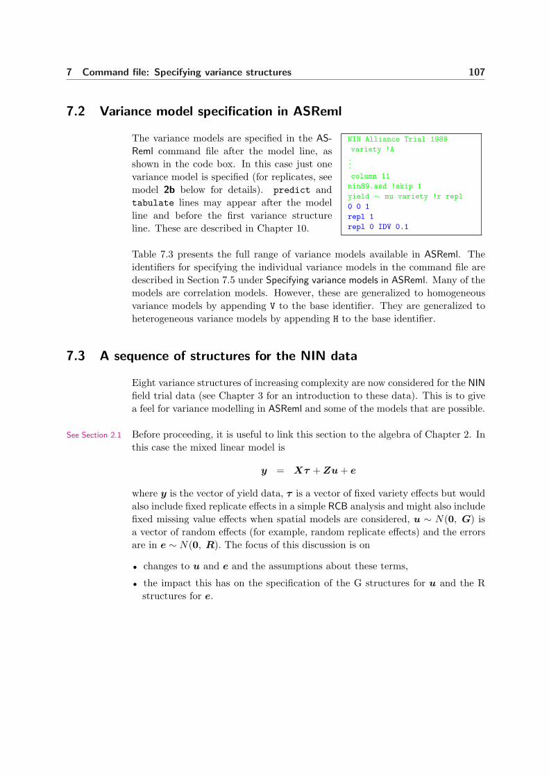
7 Command file: Specifying variance structures 107

7.2 Variance model specification in ASReml

NIN Alliance Trial 1989

variety !A...

column 11

nin89.asd !skip 1

yield ∼ mu variety !r repl

0 0 1

repl 1

repl 0 IDV 0.1

The variance models are specified in the AS-

Reml command file after the model line, asshown in the code box. In this case just onevariance model is specified (for replicates, seemodel 2b below for details). predict andtabulate lines may appear after the modelline and before the first variance structureline. These are described in Chapter 10.

Table 7.3 presents the full range of variance models available in ASReml. Theidentifiers for specifying the individual variance models in the command file aredescribed in Section 7.5 under Specifying variance models in ASReml. Many of themodels are correlation models. However, these are generalized to homogeneousvariance models by appending V to the base identifier. They are generalized toheterogeneous variance models by appending H to the base identifier.

7.3 A sequence of structures for the NIN data

Eight variance structures of increasing complexity are now considered for the NIN

field trial data (see Chapter 3 for an introduction to these data). This is to givea feel for variance modelling in ASReml and some of the models that are possible.

Before proceeding, it is useful to link this section to the algebra of Chapter 2. InSee Section 2.1

this case the mixed linear model is

y = Xτ + Zu + e

where y is the vector of yield data, τ is a vector of fixed variety effects but wouldalso include fixed replicate effects in a simple RCB analysis and might also includefixed missing value effects when spatial models are considered, u ∼ N(0, G) isa vector of random effects (for example, random replicate effects) and the errorsare in e ∼ N(0, R). The focus of this discussion is on

• changes to u and e and the assumptions about these terms,

• the impact this has on the specification of the G structures for u and the Rstructures for e.

7 Command file: Specifying variance structures 108

1 Traditional randomised complete block (RCB) analysis

NIN Alliance Trial 1989

variety !A

id

pid

raw

repl 4...

row 22

column 11

nin89.asd !skip 1

yield ∼ mu variety repl

The only random term in a traditional RCB

analysis of these data is the (residual) errorterm e ∼ N(0, σ2

eI224). The model thereforeinvolves just one R structure and no G struc-tures (u = 0). In ASReml

• the error term is implicit in the model andis not formally specified on the model line,

• the IID variance structure (R = σ2eI224) is

the default for error.

Important The error term is always present in the model but its variance structuredoes not need to be formally declared when it has the default IID structure.

2a Random effects RCB analysis

NIN Alliance Trial 1989

variety !A

id

pid

raw

repl 4...

row 22

column 11

nin89.asd !skip 1

yield ∼ mu variety !r repl

The random effects RCB model has 2 randomterms to indicate that the total variation inthe data is comprised of 2 components, a ran-dom replicate effect ur ∼ N(0, γrσ

2eI4) where

γr = σ2r/σ2

e , and error as in 1. This model in-volves both the original implicit IID R struc-ture and an implicit IID G structure for therandom replicates. In ASReml

• IID variance structure is the default for ran-dom terms in the model.

For this reason the only change to the former command file is the insertion of !rbefore repl. Important All random terms (other than error which is implicit)See Section 6.4

must be written after !r in the model specification line(s).

7 Command file: Specifying variance structures 109

2b Random effects RCB analysis with a G structure specified

NIN Alliance Trial 1989

variety !A

id

pid

raw

repl 4...

row 22

column 11

nin89.asd !skip 1

yield ∼ mu variety !r repl

0 0 1

repl 1

4 0 IDV 0.1

This model is equivalent to 2a but we explic-itly specify the G structure for repl, that is,ur ∼ N(0, γrσ

2eI4), to introduce the syntax.

The 0 0 1 line is called the variance headerSee Section 7.4

line. In general, the first two elements of thisline refer to the R structures and the third el-ement is the number of G structures. In thiscase 0 0 tells ASReml that there are no ex-plicit R structures but there is one G structure(1). The next two lines define the G structure.See page 120

The first line, a G structure header line, linksthe structure that follows to a term in the lin-ear model (repl) and indicates that it involvesone variance model (1) (a 2 would mean that the structure was the direct productof two variance models). The second line tells ASReml that the variance modelfor replicates is IDV of order 4 (σ2

rI4). The 0.1 is a starting value for γr = σ2r/σ2

e ;a starting value must be specified. Finally, the second element (0) on the lastline of the file indicates that the effects are in standard order. There is almostalways a 0 (no sorting) in this position for G structures. The following pointsshould be noted:

• the 4 on the final line could have been written as repl to give

repl 0 IDV 0.1

This would tell ASReml that the order or dimension of the IDV variance modelis equal to the number of levels in repl (4 in this case),

• when specifying G structures, the user should ensure that one scale parameteris present. ASReml does not automatically include and estimate a scale param-eter for a G structure when the explicit G structure does not include one. Forthis reason

– the model supplied when the G structure involves just one variance modelmust not be a correlation model (all diagonal elements equal 1),See Sections 2.1

and 7.5 – all but one of the models supplied when the G structure involves more thanone variance model must be correlation models; the other must be eitheran homogeneous or a heterogeneous variance model (see Section 7.5 for thedistinction between these models; see also 5 for an example),

• an initial value must be supplied for all parameters in G structure definitions.ASReml expects initial values immediately after the variance model identifier

7 Command file: Specifying variance structures 110

or on the next line (0.1 directly after IDV in this case),

– 0 is ignored as an initial value on the model line,– if there is no initial value after the identifier, ASReml will look on the next

line,– if ASReml does not find an initial value it will stop and give an error messageSee Chapter 14

in the .asr file,

• in this case V = σ2rZrZ

′r +σ2

eI224 which is fitted as σ2e (γrZrZ

′r + I224) where

γr is a variance ratio (γr = σ2r/σ2

e) and σ2e is the scale parameter. Thus 0.1 is

a reasonable initial value for γr regardless of the scale of the data.

3a Two-dimensional spatial model with spatial correlation in one direc-tion

NIN Alliance Trial 1989

variety !A

id

pid

raw

repl 4...

row 22

column 11

nin89aug.asd !skip 1

yield ∼ mu variety !f mv

1 2 0

11 column ID

22 row AR1 0.3

This code specifies a two-dimensional spatialstructure for error but with spatial correla-tion in the row direction only, that is, e ∼N(0, σ2

eI11 ⊗ Σr(ρr)). The variance headerline tells ASReml that there is one R struc-ture (1) which is a direct product of two vari-ance models (2); there are no G structures (0).The next two lines define the components ofSee page 118

the R structure. A structure definition linemust be specified for each component. ForV = σ2

eI11⊗Σ(ρr), the first matrix is an iden-tity matrix of order 11 for columns (ID), thesecond matrix is a first order autoregressivecorrelation matrix of order 22 for rows (AR1) and the variance scale parameterσ2

e is implicit. Note the following:

• placing column and row in the second position on lines 1 and 2 respectivelytells ASReml to internally sort the data rows within columns before processingthe job. This is to ensure that the data matches the direct product structurespecified. If column and row were replaced with 0 in these two lines, ASReml

would assume that the data were already sorted in this order (which is nottrue in this case),

• the 0.3 on line 2 is a starting value for the autoregressive row correlation. Notethat for spatial analysis in two dimensions using a separable model, a completematrix or array of plots must be present. To achieve this we augmented thedata with the 18 records for the missing yields as shown on page 30. In the

7 Command file: Specifying variance structures 111

augmented data file the yield data for the missing plots have all been madeNA (one of the missing value indicators in ASReml) and variety has beenarbitrarily coded LANCER for all of the missing plots (any of the variety namescould have been used),

• !f mv is now included in the model specification. This tells ASReml to estimatethe missing values. The !f before mv indicates that the missing values are fixedSee Chapter 13

effects in the sparse set of terms,See Sections 6.3

and 6.11 • unlike the case with G structures, ASReml automatically includes and esti-mates a scale parameter for R structures (σ2

e for V = σ2e (I11 ⊗Σ(ρr)) in this

case). This is why the variance models specified for row (AR1) and column(ID) are correlation models. The user could specify a non-correlation modelSee Sections 2.1

and 7.5 (diagonal elements 6= 1) in the R structure definition, for example, ID couldbe replaced by IDV to represent V = σ2

e(σ2cI11)⊗Σ(ρr). However, IDV would

then need to be followed by !S2==1 to fix σ2e at 1 and prevent ASReml trying

(unsuccessfully) to estimate both parameters as they are confounded: the scaleSee Section 7.7

parameter associated with IDV and the implicit error variance parameter, seeSection 2.1 under Combining variance models. Specifically, the code

11 column IDV 48 !S2==1

would be required in this case, where 48 is the starting value for the variances.This complexity allows for heterogeneous error variance.

3b Two-dimensional separable autoregressive spatial model

NIN Alliance Trial 1989

variety !A

id...

row 22

column 11

nin89aug.asd !skip 1

yield ∼ mu variety !f mv

1 2 0

11 column AR1 0.3

22 row AR1 0.3

This model extends 3a by specifying a firstorder autoregressive correlation model of or-der 11 for columns (AR1). The R structurein this case is therefore the direct product oftwo autoregressive correlation matrices thatis, V = σ2

eΣc(ρc) ⊗ Σr(ρr), giving a two-dimensional first order separable autoregres-sive spatial structure for error. The startingcolumn correlation in this case is also 0.3.Again note that σ2

e is implicit.

7 Command file: Specifying variance structures 112

3c Two-dimensional separable autoregressive spatial model with mea-surement error

NIN Alliance Trial 1989

variety !A

id...

row 22

column 11

nin89aug.asd !skip 1

yield ∼ mu variety !r units,

!f mv

1 2 0

11 column AR1 0.3

22 row AR1 0.3

This model extends 3b by adding a randomunits term. ThusV = σ2

e (γηI242 + Σc(ρc)⊗Σr(ρr)) . The re-served word units tells ASReml to constructan additional random term with one level foreach experimental unit so that a second (in-dependent) error term can be fitted. A unitsterm is fitted in the model in cases like this,where a variance structure is applied to theerrors. Because a G structure is not explic-itly specified here for units, the default IDVstructure is assumed. The units term is often fitted in spatial models for fieldtrial data to allow for a nugget effect.

4 Two-dimensional separable autoregressive spatial model with randomreplicate effects

NIN Alliance Trial 1989

variety !A

id...

row 22

column 11

nin89aug.asd !skip 1

yield ∼ mu variety !r repl,

!f mv

1 2 1

11 column AR1 0.3

22 row AR1 0.3

repl 1

repl 0 IDV 0.1

This is essentially a combination of 2b and 3cto demonstrate specifying an R structure anda G structure in the same model. The varianceSee Section 7.4

header line 1 2 1 indicates that there is one Rstructure (1) that involves two variance mod-els (2) and is therefore the direct product oftwo matrices, and there is one G structure (1).The R structures are defined first so the nexttwo lines are the R structure definition linesfor e, as in 3b. The last two lines are the Gstructure definition lines for repl, as in 2b. Inthis case V = σ2

e (γrI242 + Σc(ρc)⊗Σr(ρr)) .

7 Command file: Specifying variance structures 113

5 Two-dimensional separable autore-gressive spatial model defined as a G structure

NIN Alliance Trial 1989

variety !A

id...

row 22

column 11

nin89.asd !skip 1

yield ∼ mu variety,

!r row.column

0 0 1

row.column 2

row 0 AR1V 0.3 0.1

column 0 AR1 0.3

This model is equivalent to 3c but with thespatial model defined as a G structure ratherthan an R structure. As discussed in 2b,

• all but one of the models supplied when theSee Section 7.7

G structure involves more than one variancemodel must be correlation models,

• the other model must not be a correlationmodel, that is, the other model must beeither an homogeneous or a heterogeneousvariance model, and an initial value for thescale parameter must be supplied.

For this reason, the model for rows is now AR1V and an initial value of 0.1 has beensupplied for the scale parameter. In this case V = σ2

e (γrcΣc(ρc)⊗Σr(ρr) + I224) .

Use of row.column as a G structure is a useful approach for analysing incompletespatial arrays. This approach will often run faster for large trials but requiresmore memory.

Note that we have used the original version of the data and !f mv is omittedImportant

from this analysis since row.column is fitted as a G structure. If we had usedthe augmented data nin89aug.asd we would still omit !f mv and ASReml woulddiscard the records with missing yield.

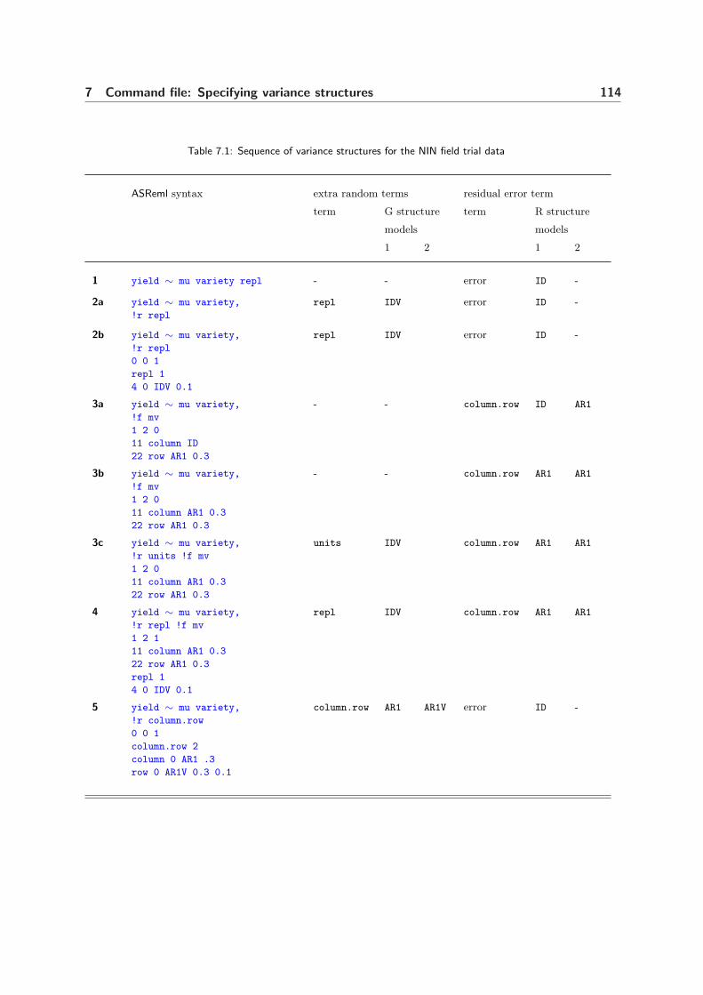
7 Command file: Specifying variance structures 114

Table 7.1: Sequence of variance structures for the NIN field trial data

ASReml syntax extra random terms residual error term

term G structure term R structure

models models

1 2 1 2

1 yield ∼ mu variety repl - - error ID -

2a yield ∼ mu variety,

!r repl

repl IDV error ID -

2b yield ∼ mu variety,

!r repl

0 0 1

repl 1

4 0 IDV 0.1

repl IDV error ID -

3a yield ∼ mu variety,

!f mv

1 2 0

11 column ID

22 row AR1 0.3

- - column.row ID AR1

3b yield ∼ mu variety,

!f mv

1 2 0

11 column AR1 0.3

22 row AR1 0.3

- - column.row AR1 AR1

3c yield ∼ mu variety,

!r units !f mv

1 2 0

11 column AR1 0.3

22 row AR1 0.3

units IDV column.row AR1 AR1

4 yield ∼ mu variety,

!r repl !f mv

1 2 1

11 column AR1 0.3

22 row AR1 0.3

repl 1

4 0 IDV 0.1

repl IDV column.row AR1 AR1

5 yield ∼ mu variety,

!r column.row

0 0 1

column.row 2

column 0 AR1 .3

row 0 AR1V 0.3 0.1

column.row AR1 AR1V error ID -

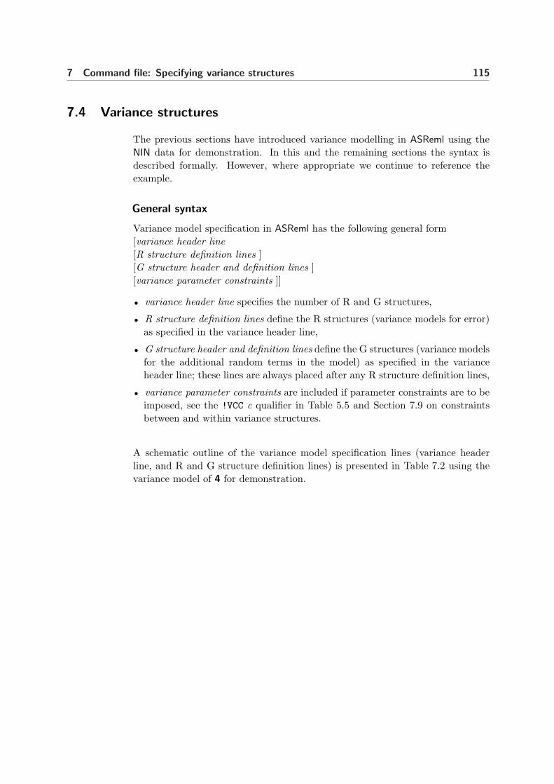
7 Command file: Specifying variance structures 115

7.4 Variance structures

The previous sections have introduced variance modelling in ASReml using theNIN data for demonstration. In this and the remaining sections the syntax isdescribed formally. However, where appropriate we continue to reference theexample.

General syntax

Variance model specification in ASReml has the following general form[variance header line[R structure definition lines ][G structure header and definition lines ][variance parameter constraints ]]

• variance header line specifies the number of R and G structures,

• R structure definition lines define the R structures (variance models for error)as specified in the variance header line,

• G structure header and definition lines define the G structures (variance modelsfor the additional random terms in the model) as specified in the varianceheader line; these lines are always placed after any R structure definition lines,

• variance parameter constraints are included if parameter constraints are to beimposed, see the !VCC c qualifier in Table 5.5 and Section 7.9 on constraintsbetween and within variance structures.

A schematic outline of the variance model specification lines (variance headerline, and R and G structure definition lines) is presented in Table 7.2 using thevariance model of 4 for demonstration.

7 Command file: Specifying variance structures 116

Table 7.2: Schematic outline of variance model specification in ASReml

general syntax model 4

variance header line [s [c [g]]] 1 2 1

- - - - - - - - - - - - - - - - - - - - - - - - - - - - - - - - - - - - - - - - - - - - - - - - - - - - - - - - - - - - -R structure definition lines S 1 C 1

C 2...C c

11 column AR1 0.3

22 row AR1 0.3...

-

S 2 C 1...C c

-...

-

......

...

S s C 1...C c

-...

-

- - - - - - - - - - - - - - - - - - - - - - - - - - - - - - - - - - - - - - - - - - - - - - - - - - - - - - - - - - - - -G structure definition lines G 1 repl 1

4 0 IDV 0.1

G 2 -

......

G g -

7 Command file: Specifying variance structures 117

Variance header line

NIN Alliance Trial 1989

variety !A

id...

row 22

column 11

nin89aug.asd !skip 1

yield ∼ mu variety !r repl,

!f mv

1 2 1

22 row AR1 0.3

11 column AR1 0.3

repl 1

repl 0 IDV 0.1

The variance header line is of the form[s [c [g]]]

• s and c relate to the R structures, g is thenumber of G structures,

• the variance header line may be omittedif the default IID R structure is required,no G structures are being explicitly definedand there are no parameter constraints (see!VCC and examples 1 and 2a),

• s is used to code the number of independentsections in the error term

– if s = 0, the default IID R structure is assumed and no R structure definitionlines are required (as in examples 2b and 5),

– if s > 0, s R structure definitions are required, one for each of the s sections(as in examples 3a, 3b, 3c and 4),

– for the analysis of multi-section data s can be replaced by the name of afactor with the appropriate number of levels, one for each section,

• c is the number of component variance models involved in the variance struc-ture for the error term for each section; for example, 3a, 3b and 3c havecolumn.row as the error term and the variance structure for column.row in-volves 2 variance models, the first for column and the second for row,

– c has a default value of 2 when s is not specified as zero,

• g is the number of variance structures (G structures) that will be explicitlyspecified for the random terms in the model.

R and G structures are now discussed with reference to s, c and g. As alreadynoted, each variance structure may involve several variance models which relateto the individual terms involved in the random effect or error. For example, atwo factor interaction may have a variance model for each of the two factorsinvolved in the interaction. Variance models are listed in Table 7.3. As indicatedSee Table 7.3

in the discussion of 2b, care must be taken with respect to scale parameters whenSee Section 7.7

combining variance models (see also Section 7.7).

7 Command file: Specifying variance structures 118

R structure definition

For each of the s sections there must be c R structure definitions. Each definitionmay take several lines. Each R structure definition specifies a variance model andhas the form

NIN Alliance Trial 1989

variety !A...

row 22

column 11

nin89aug.asd !skip 1

yield ∼ mu variety !r repl,

!f mv

1 2 1

11 column AR1 0.3

22 row AR1 0.3

repl 1

repl 0 IDV 0.1

order [field model [initial values] [qualifiers][additional initial values]]

• order is either the number of levels in thecorresponding term or the name of a factorthat has the same number of levels as theterm, for example,

11 column AR1 0.5

is equivalent to

column column AR1 0.5

when column is a factor with 11 levels,

• field is the name of the data field (variate or factor) that corresponds to theterm and therefore indexes the levels of the term;

– ASReml uses this field to sort the units so they match the R structure,– in the example the data will be sorted internally rows within columns for

the analysis but the residuals will be printed in the .yht file in the originalorder (which is actually rows within columns in this case).Important It is assumed that the joint indexing of the components uniquelydefines the experimental units,

– if field is a variable, it can be plot coordinates provided the plots are in aregular grid. Thus in this example

11 lat AR1 0.322 long AR1 0.3

is valid because lat gives column position and long gives row position, andthe positions are on a regular grid. The autoregressive correlation values willstill be on an plot index basis (1, 2, 3, . . . ), not on a distance basis (10m,20m, 30m, . . . ),

– if the data is sorted appropriately for the order the models are specified, setfield to 0,

7 Command file: Specifying variance structures 119

• model specifies the variance model for the term, for example,

22 row AR1 0.3

chooses a first order autoregressive model for the row error process,

– all the variance models available in ASReml are listed in Table 7.3,– these models have associated variance parameters,– a error variance component (σ2

e for the example, see Section 7.3) is auto-matically estimated for each section,

– the default model is ID,

• initial values are initial or starting values for the variance parameters and mustbe supplied, for example,

22 row AR1 0.3

chooses an autoregressive model for the row error process (see Table 7.1) witha starting value of 0.3 for the row correlation,

• qualifiers tell ASReml to modify the variance model in some way; the qualifiersare described in Table 7.4,

• additional initial values are read from the following lines if there are not enoughinitial values on the model line. Each variance model has a certain number ofparameters. If insufficient non zero values are found on the model line ASReml

expects to find them on the following line(s),

– initial values of 0.0 will be ignored if they are on the model line but areaccepted on subsequent lines,

– the notation n*v (for example, 5 * 0.1) is permitted on subsequent lines(but not the model line) when there are n repeats of a particular initial valuev,

– only in a few specified cases is 0 permitted as an initial value of a non-zeroparameter.

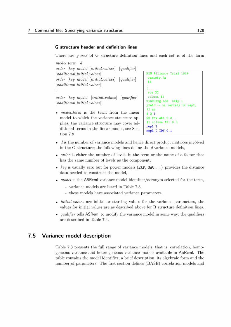
7 Command file: Specifying variance structures 120

G structure header and definition lines

There are g sets of G structure definition lines and each set is of the form

NIN Alliance Trial 1989

variety !A

id...

row 22

column 11

nin89aug.asd !skip 1

yield ∼ mu variety !r repl,

!f mv

1 2 1

22 row AR1 0.3

11 column AR1 0.3

repl 1

repl 0 IDV 0.1

model term dorder [key model [initial values] [qualifier][additional initial values]]order [key model [initial values] [qualifier][additional initial values]]...order [key model [initial values] [qualifier][additional initial values]]

• model term is the term from the linearmodel to which the variance structure ap-plies; the variance structure may cover ad-ditional terms in the linear model, see Sec-tion 7.8

• d is the number of variance models and hence direct product matrices involvedin the G structure; the following lines define the d variance models,

• order is either the number of levels in the term or the name of a factor thathas the same number of levels as the component,

• key is usually zero but for power models (EXP, GAU,. . . ) provides the distancedata needed to construct the model,

• model is the ASReml variance model identifier/acronym selected for the term,

– variance models are listed in Table 7.3,– these models have associated variance parameters,

• initial values are initial or starting values for the variance parameters, thevalues for initial values are as described above for R structure definition lines,

• qualifier tells ASReml to modify the variance model in some way; the qualifiersare described in Table 7.4.

7.5 Variance model description

Table 7.3 presents the full range of variance models, that is, correlation, homo-geneous variance and heterogeneous variance models available in ASReml. Thetable contains the model identifier, a brief description, its algebraic form and thenumber of parameters. The first section defines (BASE) correlation models and

7 Command file: Specifying variance structures 121

in the next section we show how to extend them to form variance models. Thesecond section defines some models parameterized as variance/covariance matri-ces rather than as correlation matrices. The third section covers some specialcases where the covariance structure is known except for the scale.

Table 7.3: Details of the variance models available in ASReml

baseidentifier

description algebraicform

number of parameters†

corr homo’s hetero’svariance variance

Correlation models

One-dimensional, equally spaced

ID identity Cii = 1, Cij = 0, i 6= j 0 1 ω

AR[1] 1st

orderautoregressive

Cii = 1, Ci+1,i = φ1

Cij = φ1Ci−1,j , i > j + 1

|φ1 | < 1

1 2 1 + ω

AR2 2nd

orderautoregressive

Cii = 1,

Ci+1,i = φ1/(1− φ2)

Cij = φ1Ci−1,j +φ2Ci−2,j , i > j +1

|φ1 | < (1− φ2), |φ2 | < 1

2 3 2 + ω

AR3

New3

rd

orderautoregressive

Cii = 1, Ω = 1− φ2 − φ3(φ1 + φ3),

Ci+1,i = (φ1 + φ2φ3)/Ω,

3 4 3 + ω

Ci+2,i = (φ1(φ1 + φ3) + φ2(1− φ2))/Ω,

Cij = φ1Ci−1,j + φ2Ci−2,j + φ3Ci−3,j , i > j + 2

|φ1 | < (1− φ2), |φ2 | < 1, |φ3 | < 1

SAR symmetricautoregressive

Cii = 1,

Ci+1,i = φ1/(1 + φ21/4)

Cij = φ1Ci−1,j − φ21/4 Ci−2,j ,

i > j + 1

|φ1 | < 1

1 2 1 + ω

SAR2

Newconstrainedautoregressive 3used forcompetition

as for AR3 using

φ1 = γ1 + 2γ2 ,

φ2 = −γ2(2γ1 + γ2),

φ3 = γ1γ22 ,

2 3 2 + ω

7 Command file: Specifying variance structures 122

Details of the variance models available in ASReml

baseidentifier

description algebraicform

number of parameters†

corr homo’s hetero’svariance variance

MA[1] 1st

ordermoving average

Cii = 1,

Ci+1,i = −θ1/(1 + θ21)

Cji = 0, j > i + 2

|θ1 | < 1

1 2 1 + ω

MA2 2nd

ordermoving average

Cii = 1,

Ci+1,i = −θ1(1− θ2)/(1 + θ21 + θ2

2)

Ci+2,i = −θ2/(1 + θ21 + θ2

2)

Cji = 0, j > i + 2

θ2 ± θ1 < 1

|θ1 | < 1, |θ2 | < 1

2 3 2 + ω

ARMA autoregressivemoving average

Cii = 1,

Ci+1,i = (θ − φ)(1− θφ)/(1 +

θ2 − 2θφ)

Cji = φCj−1,i , j > i + 1

|θ| < 1, |φ| < 1

2 3 2 + ω

CORU uniformcorrelation

Cii = 1, Cij = φ, i 6= j 1 2 1 + ω

CORB bandedcorrelation

Cii = 1

Ci+j,i = φj , 1 ≤ j ≤ ω − 1

|φj | < 1

ω − 1 ω 2ω − 1

CORG generalcorrelationCORGH = US

Cii = 1

Cij = φij , i 6= j

|φij | < 1

ω(ω−1)2

ω(ω−1)2

+1 ω(ω−1)2

+ ω

One-dimensional unequally spaced

EXP exponential Cii = 1

Cij = φ|xi−xj |, i 6= j

xi are coordinates0 < φ < 1

1 2 1 + ω

7 Command file: Specifying variance structures 123

Details of the variance models available in ASReml

baseidentifier

description algebraicform

number of parameters†

corr homo’s hetero’svariance variance

GAU gaussian Cii = 1

Cij = φ(xi−xj)2 , i 6= j

xi are coordinates

0 < φ < 1

1 2 1 + ω

Two-dimensional irregularly spaced

x and y vectors of coordinates

θij = min(dij/φ1, 1)

dij is euclidean distance

IEXP isotropic

exponential

Cii = 1

Cij = φ|xi−xj |+|yi−yj |, i 6= j

0 < φ < 1

1 2 1 + ω

IGAU isotropic

gaussian

Cii = 1

Cij = φ(xi−xj)2+(yi−yj)2 , i 6= j

0 < φ < 1

1 2 1 + ω

IEUC isotropic

euclidean

Cii = 1

Cij = φ√

(xi−xj)2+(yi−yj)2 , i 6= j

0 < φ < 1

1 2 1 + ω

LVR

Newlinear variance Cij = (1− θij)

0 < φ1

1 2 1 + ω

SPH

Newspherical Cij = 1− 3

2θij + 1

2θ3

ij

0 < φ1

1 2 1 + ω

CIR

Newcircular (Web-

ster & Oliver,

2001, p 113)

Cij = 1

− 2π(θij

√1− θ2

ij + sin−1θij)

0 < φ1

1 2 1 + ω

AEXP anisotropic ex-ponential

Cii = 1

Cij = φ|xi−xj |1 φ

|yi−yj |2

0 < φ1 < 1, 0 < φ2 < 1

2 3 2+ω

7 Command file: Specifying variance structures 124

Details of the variance models available in ASReml

baseidentifier

description algebraicform

number of parameters†

corr homo’s hetero’svariance variance

AGAU anisotropicgaussian

Cii = 1

Cij = φ(xi−xj)2

1 φ(yi−yj)2

2

0 < φ1 < 1, 0 < φ2 < 1

2 3 2 + ω

MATkNew

Matern withfirst 1 ≤ k ≤ 5parametersspecified by theuser

Cij =Matern: see text

φ > 0 range, ν shape(0.5)

δ > 0 anisotropy ratio(1),

α anisotropy angle(0),

λ(1|2) metric(2)

k k+1 k + ω

Additional heterogeneous variance models

DIAG diagonal = IDH Σii = φi Σij = 0, i 6= j - - ω

US unstructuredgeneral covari-ance matrix

Σij = φij - -ω(ω+1)

2

OWNk user explicitlyforms V and∂V

- - k

ANTE[1]

ANTEk1

st

kth

k orderantede-pendence

1 ≤ k ≤ ω − 1

Σ−1

= UDU ′

Dii = di , Dij = 0, i 6= j

Uii = 1, Uij = uij , 1 ≤ j − i ≤ k

U ij = 0, i > j

- -ω(ω+1)

2

CHOL[1]

CHOLk1

st

kth

k ordercholesky(bandedform)

1 ≤ k ≤ ω − 1

Σ = LDL′

Dii = di , Dij = 0, i 6= j

Lii = 1, Lij = lij , 1 ≤ i− j ≤ k;Lij = 0, i− j > k;

- -ω(ω+1)

2

CHOL[1]C

CHOLkC1

st

kth

k ordercholesky(columnform)

1 ≤ k ≤ ω − 1

Σ = LDL′

Dii = di , Dij = 0, i 6= j

Lii = 1, Lij = lij , 1 ≤ j < i;Lij = 0., k + 1 ≤ j < i;

- -ω(ω+1)

2

7 Command file: Specifying variance structures 125

Details of the variance models available in ASReml

baseidentifier

description algebraicform

number of parameters†

corr homo’s hetero’svariance variance

FA[1]

FAk1

st

kth

k orderfactoranalytic

Σ = DCD,C = FF ′ + E,F contains k correlation factorsE diagonalDD = diag (Σ)

- - ω + ωkω + ω

FACV[1]

FACVk1

st

kth

k orderfactoranalyticcovarianceform

Σ = ΓΓ′ + Ψ,Γ contains covariance factorsΨ contains specific variance

- - ω + ωkω + ω

XFA[1]

XFAk1

st

kth

k orderextendedfactoranalyticcovarianceform

Σ = ΓΓ′ + Ψ,Γ contains covariance factorsΨ contains specific variance

- - ω + ωkω + ω

Inverse relationship matrices‡

AINV inverse relationship matrix derived from pedigree 0 1 -

GIV1 generalized inverse number 1 0 1 -

......

......

...

GIV6 generalized inverse number 6 0 1 -

† This is the number of values the user must supply as initial values where ω is the dimension of thematrix. The homogeneous variance form is specified by appending V to the correlation basename; theheterogeneous variance form is specified by appending H to the correlation basename‡ These must be associated with 1 variance parameter unless used in direct product with another structurewhich provides the variance.

7 Command file: Specifying variance structures 126

Forming variance models from correlation models

The base identifiers presented in the first part of Table 7.3 are used to specify thecorrelation models. The corresponding homogeneous and heterogeneous variancemodels are specified by appending V and H to the base identifiers respectively.This convention holds for most models. However, no V or H should be appendedto the base identifiers for the heterogeneous variance models at the end of thetable (from DIAG on).

In summary, to specify

• a correlation model, provide the base identifier given in Table 7.3, for example

EXP .1

is an exponential correlation model,

• an homogeneous variance model, append a V to the base identifier and providean additional initial value for the variance, for example,

EXPV .1 .3

is an exponential variance model,

• a heterogeneous variance model, append an H to the base identifier and provideadditional initial values for the diagonal variances, for example,

CORUH .1 .3 .4 .2

is a 3× 3 matrix with uniform correlations of 0.1 and heterogeneous variances0.3, 0.4 and 0.2.

Important See Section 7.7 for rules on combining variance models and importantnotes regarding initial values.

The algebraic forms of the homogeneous and heterogeneous variance models aredetermined as follows. Let C (ω×ω) = [Cij ] denote the correlation matrix fora particular correlation model. If Σ (ω×ω) is the corresponding homogeneousvariance matrix then

Σ = σ2C.

It has just one more parameter than the correlation model. For example, thehomogeneous variance model corresponding to the ID correlation model has vari-ance matrix Σ = σ2Iω (specified IDV in the ASReml command file, see below)and one parameter. The initial values for the variance parameters are listed afterthe initial values for the correlation parameters. For example, in

7 Command file: Specifying variance structures 127

AR1V 0.3 0.5

0.3 is the initial spatial correlation parameter and 0.5 is the initial varianceparameter value.

Similarly, if Σ (ω×ω)h is the heterogeneous variance matrix corresponding to C,

then

Σh = DCD

where D (ω×ω) = diag (σi) . In this case there are an additional ω parameters.For example, the heterogeneous variance model corresponding to ID is specifiedIDH in the ASReml command file (see below), involves the ω parameters σ2

1. . . σ2

ω

and is the variance matrix

Σh =

σ21

0 . . . 00 σ2

2. . . 0

......

. . ....

0 0 . . . σ2ω

Notes on the variance models

These notes provide additional information on the variance models defined inTable 7.3.

• the IDH and DIAG models fit the same diagonal variance structure,

• the CORGH and US models fit the same completely general variance structureparameterized differently,

• in CHOLk models Σ = LDL′ where L is lower triangular with ones on thediagonal, D is diagonal and k is the number of non-zero off diagonals in L,

• in CHOLkC models Σ = LDL′ where L is lower triangular with ones on theNew

diagonal, D is diagonal and k is the number of non-zero sub diagonal columnsin L. This is somewhat similar to the factor analytic model.

• in ANTEk models Σ−1 = UDU ′ where U is upper triangular with ones on thediagonal, D is diagonal and k is the number of non-zero off diagonals in U ,

• the CHOLk, CHOLkC and ANTEk models are equivalent to the US structure, thatis, the full variance structure, when k is ω − 1,

• initial values for US, CHOLk CHOLkC and ANTEk structures are given in the formof a US matrix which is specified lower triangle row-wise, viz

7 Command file: Specifying variance structures 128

σ11

σ21 σ22

σ31 σ32 σ33

,

that is, initial values are given in the order, 1 = σ11 , 2 = σ21 , 3 = σ22 , . . .

• the US model is associated with several special features of ASReml. Whenused in the R structure for multivariate data, ASReml automatically recognisespatterns of missing values in the responses (see Chapter 8). Also, there is anoption to update its values by EM rather than AI when its AI updates makethe matrix non positive definite.

• The Matern class of isotropic covariance models is now described. ASRemlNew

uses an extended Matern class which accomodates geometric anisotropy and achoice of metrics for random fields observed in two dimensions. This extension,described in detail in Haskard (2006), is given by

ρ(h;φ) = ρM (d(h; δ, α, λ);φ, ν)

where h = (hx, hy)T is the spatial separation vector, (δ, α) governs geometricanisotropy, (λ) specifies the choice of metric and (φ, ν) are the parameters ofthe Matern correlation function. The function is

ρM (d; φ, ν) =2ν−1Γ(ν)

−1(

d

φ

)ν

Kν

(d

φ

), (7.1)

where φ > 0 is a range parameter, ν > 0 is a smoothness parameter, Γ(·) is thegamma function, Kν(.) is the modified Bessel function of the third kind of orderν (Abramowitz and Stegun, 1965, section 9.6) and d is the distance defined interms of X and Y axes: hx = xi − xj ; hy = yi − yj ; sx = cos(α)hx + sin(α)hy;sy = cos(α)hx − sin(α)hy; d = (δ|sx|λ + |sy|λ/δ)1/λ.

For a given ν, the range parameter φ affects the rate of decay of ρ(·) withincreasing d. The parameter ν > 0 controls the analytic smoothness of theunderlying process us, the process being dνe − 1 times mean-square differen-tiable, where dνe is the smallest integer greater than or equal to ν (Stein, 1999,page 31). Larger ν correspond to smoother processes. ASReml uses numericalderivatives for ν when its current value is outside the interval [0.2,5].

When ν = m + 12 with m a non-negative integer, ρM (·) is the product of

exp(−d/φ) and a polynomial of degree m in d. Thus ν = 12 yields the exponen-

tial correlation function, ρM (d; φ, 12) = exp(−d/φ), and ν = 1 yields Whittle’s

elementary correlation function, ρM (d; φ, 1) = (d/φ)K1(d/φ) (Webster andOliver, 2001).

When ν = 1.5 then

ρM (d;φ, 1.5) = exp(−d/φ)(1 + d/φ)

7 Command file: Specifying variance structures 129

which is the correlation function of a random field which is continuous and oncedifferentiable. This has been used recently by Kammann and Wand (2003).As ν →∞ then ρM (·) tends to the gaussian correlation function.

The metric parameter λ is not estimated by ASReml ; it is usually set to 2for Euclidean distance. Setting λ = 1 provides the cityblock metric, whichtogether with ν = 0.5 models a separable AR1×AR1 process. Cityblock met-ric may be appropriate when the dominant spatial processes are aligned withrows/columns as occurs in field experiments. Geometric anisotropy is discussedin most geostatistical books (Webster and Oliver, 2001, Diggle et al., 2003) butrarely are the anisotropy angle or ratio estimated from the data. Similarly thesmoothness parameter ν is often set a-priori (Kammann and Wand, 2003, Dig-gle et al., 2003). However Stein (1999) and Haskard (2006) demonstrate thatν can be reliably estimated even for modest sized data-sets, subject to caveatsregarding the sampling design.

The syntax for the Matern class in ASReml is given by MATk where k is thenumber of parameters to be specified; the remaining parameters take theirdefault values. Use the !G qualifier to control whether a specified parameter isestimated or fixed. The order of the parameters in ASReml, with their defaults,is (φ, ν = 0.5, δ = 1, α = 0, λ = 2). For example, if we wish to fit a Maternmodel with only φ estimated and the other parameters set at their defaultsthen we use MAT1. MAT2 allows ν to be estimated or fixed at some other value(for example MAT2 .2 1 !GPF). The parameters φ and ν are highly correlatedso it may be better to manually cover a grid of ν values.

We note that there is non-uniqueness in the anisotropy parameters of thismetric d(·) since inverting δ and adding π

2 to α gives the same distance. Thisnon-uniqueness can be removed by considering 0 ≤ α < π

2 and δ > 0, or byconsidering 0 ≤ α < π and either 0 < δ ≤ 1 or δ ≥ 1. With λ = 2, isotropyoccurs when δ = 1, and then the rotation angle α is irrelevant: correlationcontours are circles, compared with ellipses in general. With λ = 1, correlationcontours are diamonds.

• power models rely on the definition of distance for the associated term, forexample,

– the distance between time points in a one-dimensional longitudinal analysis,– the spatial distance between plot coordinates in a two-dimensional field trial

analysis.

Information for determining distances is supplied by the key argument on thestructure line.

– For one dimensional cases, key may be

7 Command file: Specifying variance structures 130

* the name of a data field containing the coordinate values when it relatesto an R structure

* 0 in which case a vector of coordinates of length order must be suppliedafter all R and G structure lines.

* fac(x) when it relates to model term fac(x).

– In two directions (IEXP, IGAU, IEUC, AEXP, AGAU, MATn) the key argumentalso depends on whether it relates to an R or G structure.* For an R structure, use the form rrcc where rr is the number of a data field

containing the coordinates for the first dimension and cc is the numberof a data field containing the coordinates for the second direction. Forexample, in the analysis of spatial data, if the x coordinate was in field 3and the y coordinate was in field 4, the second argument would be 304.

* For a G structure relating to the model term fac(x,y), use fac(x,y).For example...y ∼ mu ...!r fac(x,y) ......fac(x,y) 1fac(x,y) fac(x,y) IEUCV .7 1.3

• FAk, FACVk and XFAk are different parameterizations of the factor analyticmodel in which Σ is modelled as Σ = ΓΓ′ + Ψ where Γ (ω×k) is a matrix ofloadings on the covariance scale and Ψ is a diagonal vector of specific variances.See Smith et al. (2001) and Thompson et al. (2003) for examples of factoranalytic models in multi-environment trials. The general limitations are

– that Ψ may not include zeros except in the XFAk formulation– constraints are required in Γ for k > 1 for identifiability. Typically, one zero

is placed in the second column, two zeros in the third column, etc.– The total number of parameters fitted (kω+ω−k(k−1)/2) may not exceed

ω(ω + 1)/2.

• in FAk models the variance-covariance matrix Σ (ω×ω) is modelled on the cor-relation scale as Σ = DCD, where

– D (ω×ω) is diagonal such that DD = diag (Σ) ,

– C (ω×ω) is a correlation matrix of the form FF ′ + E where F (ω×k) is amatrix of loadings on the correlation scale and E is diagonal and is definedby difference,

– the parameters are specified in the order loadings for each factor (F ) fol-lowed by the variances (diag (Σ)); when k is greater than 1, constraints on

7 Command file: Specifying variance structures 131

the elements of F are required, see Table 7.5,

• FACVk models (CV for covariance) are an alternative formulation of FA modelsin which Σ is modelled as Σ = ΓΓ′ + Ψ where Γ (ω×k) is a matrix of loadingson the covariance scale and Ψ is diagonal. The parameters in FACV

– are specified in the order loadings (Γ) followed by variances (Ψ); when k isgreater than 1, constraints on the elements of Γ are required, see Table 7.5,

– are related to those in FA by Γ = DF and Ψ = DED,

• XFAk (X for extended) is the third form of the factor analytic model and hasdifficult

the same parameterisation as for FACV, that is, Σ = ΓΓ′ + Ψ. However, XFAmodels

– have parameters specified in the order diag (Ψ) and vec(Γ); when k is greaterthan 1, constraints on the elements of Γ are required, see Table 7.5,

– may not be used in R structures,– are used in G structures in combination with the xfa(f,k) model term,– return the factors as well as the effects.– permit some elements of Ψ to be fixed to zero,– are computationally faster than the FACV formulation for large problems

when k is much smaller than ω,

Special consideration is required when using the XFAk model. The SSP mustbe expanded to have room to hold the k factors. This is achieved by using thexfa(f,k) model term in place of f in the model. For example,y ∼ site !r geno.xfa(site,2)0 0 1geno.xfa(site,2) 2genoxfa(site,2) 0 XFA2

• the OWN variance structure is a facility whereby users may specify their own vari-difficult

ance structure. This facility requires the user to supply a program MYOWNGDGthat reads the current set of parameters, forms the G matrix and a full set ofderivative matrices, and writes these to disk. Before each iteration, ASReml

writes the OWN parameters to a file, runs MYOWNGDG (which it presumes formsthe G and derivative matrix) and then reads the matrices back in. An exampleof MYOWNGDG.f90 is distributed with ASReml. It duplicates the AR1 and AR2structures. The following job fits an AR2 structure using this program.

Example of using the OWN structurerepblcol

7 Command file: Specifying variance structures 132

blrowvariety 25yieldbarley.asd !skip 1 !OWN MYOWN.EXEy ∼ va1 210 0 AR1 .115 0 OWN2 .2 .1 !TRR

The file written by ASReml has extension .own and looks like

15 2 1

0.6025860D+000.1164403D+00

This file was written by asreml for reading by your

program MYOWNGDG

asreml writes this file, runs your program and then reads

shfown.gdg

which it presumes has the following format:

The first lines should agree with the top of this file

specifying the order of the matrices ( 15)

the number of variance parameters ( 2)

and a control parameter you can specify ( 1).

These are written in (3I5) format. They are followed by

the list of variance parameters written in (6D13.7) format.

Follow this with 3 matrices written in (6D13.7) format.

These are to be each of 120 elements being lower triangle

row-wise of the G matrix and its derivatives with respect

to the parameters in turn.

This file contains details about what is expected in the file written by yourprogram. The filename used has the same basename as the job you are run-ning with extension .own for the file written by ASReml and .gdg for the fileyour program writes. The type of the parameters is set with the !T qualifierdescribed below. The control parameter is set using the !F qualifier.

– !F2 applies to OWN models. With OWN, the argument of !F is passed to theMYOWNGDG program as an argument the program can access. This is themechanism that allows several OWN models to be fitted in a single run.

– !Ts is used to set the type of the parameters. It is primarily used in con-junction with the OWN structure as ASReml knows the type in other cases.The valid type codes are as follows:

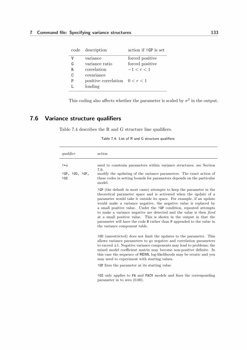
7 Command file: Specifying variance structures 133

code description action if !GP is set

V variance forced positiveG variance ratio forced positiveR correlation −1 < r < 1C covarianceP positive correlation 0 < r < 1L loading

This coding also affects whether the parameter is scaled by σ2 in the output.

7.6 Variance structure qualifiers

Table 7.4 describes the R and G structure line qualifiers.

Table 7.4: List of R and G structure qualifiers

qualifier action

!=s used to constrain parameters within variance structures, see Section7.9.

!GP, !GU, !GF,

!GZ

modify the updating of the variance parameters. The exact action ofthese codes in setting bounds for parameters depends on the particularmodel.

!GP (the default in most cases) attempts to keep the parameter in thetheoretical parameter space and is activated when the update of aparameter would take it outside its space. For example, if an updatewould make a variance negative, the negative value is replaced bya small positive value. Under the !GP condition, repeated attemptsto make a variance negative are detected and the value is then fixedat a small positive value. This is shown in the output in that theparameter will have the code B rather than P appended to the value inthe variance component table.

!GU (unrestricted) does not limit the updates to the parameter. Thisallows variance parameters to go negative and correlation parametersto exceed ±1. Negative variance components may lead to problems; themixed model coefficient matrix may become non-positive definite. Inthis case the sequence of REML log-likelihoods may be erratic and youmay need to experiment with starting values.

!GF fixes the parameter at its starting value

!GZ only applies to FA and FACV models and fixes the correspondingparameter in to zero (0.00).

7 Command file: Specifying variance structures 134

List of R and G variance structure definition line qualifiers

qualifier action

For multiple parameters, the form !GXXXX can be used to specify F,

P, U or Z for the parameters individually. A shorthand notation allowsa repeat count before a code letter. Thus !GPPPPPPPPPPPPPPZPPPZP

could be written as !G14PZ3PZP.

For a US model, !GP makes ASReml attempt to keep the matrix posi-tive definite. After each AI update, it extracts the eigenvalues of theupdated matrix. If any are negative or zero, the AI update is discardedand an EM update is performed. Notice that the EM update is appliedto all of the variance parameters in the particular US model and cannotbe applied to only a subset of them.

!S2=r sets the initial value of the error variance within the section to r: the!S2= qualifier may be used in R structure definitions to represent theresidual variance associated with the particular section. There is alwaysan error variance parameter associated with a section R structure. Inmultiple section analyses the !S2= qualifier is used on the first of the clines for each section to set the initial error variance for that section. Ifthis is not supplied, ASReml calculates an initial value that is half thesimple variance of the data in the site. To fix the variance !S2==r isused.

!S2==r is similar to !S2= except that the variance is fixed at r.

!S2==1 is used in the analysis of multiple section data and in multivariateanalyses and when variance parameters are included in the R structure.

7.7 Rules for combining variance models

As noted in Section 2.1 under Combining variance models, variance structuresare sometimes formed by combining variance models. For example, a two factorinteraction may involve two variance models, one for each of the two factors inthe interaction. Some of the rules for combining variance models differ for Rstructures and G structures.

7 Command file: Specifying variance structures 135

NIN Alliance Trial 1989

variety !A

id...

row 22

column 11

nin89.asd !skip 1

yield ∼ mu variety !r repl,

column.row

0 0 1

column.row 2

column 0 AR1 0.4

row 0 ARV1 0.3 0.1

A summary of the rules is as follows:

• when combining variance models in both Rand G structures, the resulting direct prod-uct structure must match the ordered ef-fects with the outer factor first, for example,the G structure in the example opposite isfor column.row which tells ASReml that thedirect product structure matches the effectsordered rows within columns. (The variancemodel can be written as σ2(I +ΣC⊗λΣR).)This is why the G structure definition linefor column is specified first,

• ASReml automatically includes and estimates an error variance parameter foreach section of an R structure. The variance structures defined by the usershould therefore normally be correlation matrices. A variance model can bespecified but the !S2==1 qualifier would then be required to fix the error vari-ance at 1 and prevent ASReml trying to estimate two confounded parameters(error variance and the parameter corresponding to the variance model speci-fied, see 3a on page 111),

• ASReml does not have an implicit scale parameter for G structures that aredefined explicitly. For this reason the model supplied when the G structureinvolves just one variance model must be a variance model; an initial valueSee Sections 2.1

and 7.5 must be supplied for this associated scale parameter; this is discussed underadditional initial values on page 119,

• when the G structure involves more than one variance model, one must beeither a homogeneous or a heterogeneous variance model and the rest shouldbe correlation models; if more than one are non-correlation models then the!GF qualifier should be used to avoid identifiability problems, that is, ASReml

trying to estimate both parameters when they are confounded.

7.8 G structures involving more than one random term

The usual case is that a variance structure applies to a particular term in thelinear model and that there is no covariance between model terms. Sometimes itis appropriate to include a covariance. Then, it is essential that the model termsbe listed together and that the variance structure defined for the first term be thestructure required for both terms. When the terms are of different size, the termsmust be linked together with the ! and ! qualifiers (Table 6.1). While ASReml

7 Command file: Specifying variance structures 136

will check the overall size, it does not check that the order of effects matches thestructure definition so the user must be careful to get this right. Check that theterms are conformable by considering the order of the fitted effects and ensuringCheck the order

the first term of the direct product corresponds to the outer factor in the nestingof the effects. Two examples are

• random regressions where we want a covariance between intercept and slope...!r ! animal animal.time !...animal 22 0 US 3 -.5 2animal

is equivalent (though not identical because of the scaling differences) to...!r pol(time,1).animal...pol(time,1).animal 2pol(time,1) 0 US 1 -.1 .2animal

• maternal/direct genetic covariance

lambid !Psireid !Pdamid !P...wwt ywt ∼ Trait Trait.sex !r ! Trait.lambid at(Trait,2).damid !...Trait.lambid 23 0 US1.3 # Var(wwt D)1.0 2.2 # Cov(wwt D,ywt D) Var(ywt D)-.1 -.2 0.8 # Cov(wwt D,wwt M) Cov(ywt D,wwt M) Var(wwt M)lambid 0 AINV # AINV explicitly requests to use A inverse

7 Command file: Specifying variance structures 137

7.9 Constraining variance parameters

Parameter equality within and between variance structures

Equality of parameters in a variance model can be specified using the !=s qualifierdifficult

where s is a string of letters and/or zeros (see Table 7.4). Positions in the stringcorrespond to the parameters of the variance model:

• all parameters with the same letter in the structure are treated as the sameparameter,

• 1-9 are different from a-z which are different from A-Z so that 61 equalitiescan be specified. 0 and . mean unconstrained. A colon generates a sequenceviz. a:e is the same as abcde

• Putting % as the first characterin s makes the interpretation of codes absoluteNew

(so that they apply across structures).

• Putting * as the first characterin s indicates that numbers are repeat counts,New

A-Z are equality codes and only . is unconstrained. Thus !=*.3A2. is equiv-alent to !=0AAA00 or !=0aaa00.

Examples are presented in Table 7.5.

Table 7.5: Examples of constraining variance parameters in ASReml

ASReml code action

!=ABACBA0CBA constrain all parameters correspondingto A to be equal, similarly for B and C.The 7th parameter would be left uncon-strained. This sequence applied to anunstructured 4 × 4 matrix would makeit banded, that isAB AC B A0 C B A

site.gen 2 # G header line

site 0 US .3 !=0A0AA0 !GPUPUUP

.1 .4 .1 .1 .3

gen

this example defines a structure for thegenotype by site interaction effects in aMET in which the genotypes are inde-pendent random effects within sites butare correlated across sites with equal co-variance.

7 Command file: Specifying variance structures 138

Examples of constraining variance parameters in ASReml

ASReml code action

site 0 FA2 !G4PZ3P4P !=00000000VVVV

4*.9 # initial values for 1st factor0 3*.1 # initial values for 2nd factor

# first fixed at 04*.2 # init values for site variances

a 2 factor Factor Analytic model for 4sites with equal variance is specified us-ing this syntax. The first loading in thesecond factor is constrained equal to 0for identifiability. P places restrictionson the magnitude of the loadings andthe variances to be positive.

xfa(site,2) 0 XFA2 !=VVVV0 !4P4PZ3P

4*.2 # initial specific variances4*1.2 # initial loadings for 1st factor0 3*.3 # initial loadings for 2nd factor

a 2 factor Factor analytic model inwhich the specific variances are allequal.

Constraints between and within variance models

More general relationships between variance parameters can be defined using thedifficult

!VCCc qualifier placed on the data file definition line.

• !VCC c specifies that there are c constraint lines defining constraints to beapplied,

• the constraint lines occur after the variance header line and any R and Gstructure lines, that is, there must be a variance header line,

• each constraint is specified in a separate line in the form

P1 ∗ V1 P2 ∗ V2 ...

– Pi is the name of a random model term or the number of a parameter andVi is a coefficient,

– P1 is the primary parameter number,– ∗ indicates that the next values (Vi) is a weighting coefficient,– if the coefficient is 1 you may omit the * 1,– if the coefficient is -1 you may write −Pi instead of Pi ∗ −1,– the meaning of the coefficients is as follows P2 = V2 ∗ P1/V1 ,

– typically V1 = 1,

– a variance parameter may only be included in constraints once,

7 Command file: Specifying variance structures 139

• the Pi terms refer to positions in the full variance parameter vector. This maychange if the model is changed and is often difficult to determine as a number.If it refers to a parameter which is a single traditional variance componentassociated with a random term, the name of the random term may be giveninstead of the parameter number. The full parameter vector includes a termfor each factor in the model and then a term for each parameter defined in theR and G structures. A list of Pi numbers and their initial values is returnedin the .res file to help you to check the numbers. Alternatively, examine the.asr file from an initial run with !VCC included but no arguments supplied.The job will terminate but ASReml will provide the Pi values associated witheach variance component. Otherwise the numbers are given in the .res file.

The following are examples:

ASReml code action

5 7 * .1 parameter 7 is a tenth of parameter 5

5 -7 parameter 7 is the negative of parameter 5

32 34 35 37 38 39 for a (4× 4) US matrix given by parameters 31 . . . 40,the covariances are forced to be equal.

units -uni(check) parameter associated with model term uni(check)

has the same magnitude but opposite sign to the pa-rameter associated with model term units

7.10 Model building using the !CONTINUE qualifier

In complex models, the Average Information algorithm can have difficulty max-imising the REML log-likelihood when starting values are not reasonably closeto the REML solution. ASReml has several internal strategies to cope with thisdifficult

problem but these are not always successful.

When the user needs to provide better starting values, one method is to fit asimpler variance model. For example, it can be difficult to guess reasonablestarting values for an unstructured variance matrix. A first step might be toassume independence and just estimate the variances. If all the variances are notpositive, there is little point proceeding to try and estimate the covariances.

7 Command file: Specifying variance structures 140

The !CONTINUE qualifier instructs ASReml to retrieve variance parameters fromthe .rsv file if it exists rather than using the values in the .asr file. When readingthe .rsv file, it will take results from some matrices as supplying starting valuesfor other matrices. The transitions recognised are

DIAG to CORUHDIAG to FA1CORUH to FA1FAi to FAi+1FAi to CORGHFAi to USCORGH to US

The use of the .rsv file with !CONTINUE in this way reduces the need for the userto type in the updated starting values.

The various models may be written in various !PART s of the job and controlledby the !DOPART qualifier. When used with the -r qualifier on the command line(see Chapter 12), the output from the various parts has the partnumber appendedto the filename. In this case it would be necessary to copy the .rsv files with thenew part number before running the next part to take advantage of this facility.

8 Command file: Multivariateanalysis

Introduction

Repeated measures on rats

Wether trial data

Model specification

Variance structures

Specifying multivariate variance structures in ASReml

The output for a multivariate analysis

141

8 Command file: Multivariate analysis 142

8.1 Introduction

Multivariate analysis is used here in the narrow sense of a multivariate mixedmodel. There are many other multivariate analysis techniques which are notcovered by ASReml. Multivariate analysis is used when we are interested inestimating the correlations between distinct traits (for example, fleece weightand fibre diameter in sheep) and for repeated measures of a single trait.

Repeated measures on rats

Wolfinger rat data

treat !A

wt0 wt1 wt2 wt3 wt4

rat.dat

wt0 wt1 wt2 wt3 wt4 ∼ Trait,

treat Trait.treat

1 2 0

27 0 ID #error variance

Trait 0 US

15 * 0

Wolfinger (1996) summarises a range of vari-ance structures that can be fitted to repeatedmeasures data and demonstrates the modelsusing five weights taken weekly on 27 rats sub-jected to 3 treatments. This command filedemonstrates a multivariate analysis of thefive repeated measures. Note that the two di-mensional structure for common error meetsthe requirement of independent units and iscorrectly ordered traits with units.

Wether trial data

Orange Wether Trial 1984-8

SheepID !I

TRIAL

BloodLine !I

TEAM *

YEAR *

GFW YLD FDIAM

wether.dat !skip 1

GFW FDIAM ∼ Trait Trait.YEAR,

!r Trait.TEAM Trait.SheepID

1 2 2

1485 0 ID

Trait 0 US .2 .2 .4

Trait.TEAM 2

Trait 0 US

0.4

0.3 1.3

TEAM 0 ID

Trait.SheepID 2

Trait 0 US

0.2 0.2 2

SheepID 0 ID

predict YEAR Trait

Three key traits for the Australian wool in-dustry are the weight of wool grown per year,the cleanness and the diameter of that wool.Much of the wool is produced from wethersand most major producers have traditionallyused a particular strain or bloodline. To as-sess the importance of bloodline differences,many wether trials were conducted. Onetrial was conducted from 1984 to 1988 atBorenore near Orange. It involved 35 teamsof wethers representing 27 bloodlines. Thefile wether.dat shown below contains greasyfleece weight (kg), yield (percentage of cleanfleece weight to greasy fleece weight) and fibrediameter (microns). The code (wether.as) tothe right performs a basic bivariate analysis ofthis data.

8 Command file: Multivariate analysis 143

SheepID Site Bloodline Team Year GFW Yield FD

0101 3 21 1 1 5.6 74.3 18.5

0101 3 21 1 2 6.0 71.2 19.6

0101 3 21 1 3 8.0 75.7 21.5

0102 3 21 1 1 5.3 70.9 20.8

0102 3 21 1 2 5.7 66.1 20.9

0102 3 21 1 3 6.8 70.3 22.1

0103 3 21 1 1 5.0 80.7 18.9

0103 3 21 1 2 5.5 75.5 19.9

0103 3 21 1 3 7.0 76.6 21.9...

4013 3 43 35 1 7.9 75.9 22.6

4013 3 43 35 2 7.8 70.3 23.9

4013 3 43 35 3 9.0 76.2 25.4

4014 3 43 35 1 8.3 66.5 22.2

4014 3 43 35 2 7.8 63.9 23.3

4014 3 43 35 3 9.9 69.8 25.5

4015 3 43 35 1 6.9 75.1 20.0

4015 3 43 35 2 7.6 71.2 20.3

4015 3 43 35 3 8.5 78.1 21.7

8.2 Model specification

The syntax for specifying a multivariate linear model in ASReml is

Y-variates ∼ fixed [!r random ] [!f sparse fixed ]

• Y-variates is a list of traits,

• fixed, random and sparse fixed are as in the univariate case (see Chapter 6) butinvolve the special term Trait and interactions with Trait.

The design matrix for Trait has a level (column) for each trait.

– Trait by itself fits the mean for each variate,– In an interaction Trait.Fac fits the factor Fac for each variate andTrait.Cov fits the covariate Cov for each variate.

ASReml internally rearranges the data so that n data records containing t traitseach becomes n sets of t analysis records indexed by the internal factor Trait i.e.nt analysis records ordered Trait within data record. If the data is already inthis long form, use the !ASMV t qualifier to indicate that a multivariate analysisis required.

8 Command file: Multivariate analysis 144

8.3 Variance structures

Using the notation of Chapter 7, consider a multivariate analysis with t traits andn units in which the data are ordered traits within units. An algebraic expressionfor the variance matrix in this case is

In ⊗Σ

where Σ (t×t) is an unstructured variance matrix.

Specifying multivariate variance structures in ASReml

Orange Wether Trial 1984-8

SheepID !I

TRIAL

BloodLine !I

TEAM *

YEAR *

GFW YLD FDIAM

wether.dat !skip 1

GFW FDIAM ∼ Trait Trait.YEAR,

!r Trait.TEAM Trait.SheepID

1 2 2

1485 0 ID

Trait 0 US

3*0

Trait.TEAM 2

Trait 0 US

3*0

TEAM 0 ID

Trait.SheepID 2

Trait 0 US

3*0

SheepID 0 ID

predict YEAR Trait

A more sophisticated error structure is re-quired for multivariate analysis. For a stan-dard multivariate analysis

• the error structure for the residual must bespecified as two-dimensional with indepen-dent records and an unstructured variancematrix across traits; records may have ob-servations missing in different patterns andthese are handled internally during analy-sis,

• the R structure must be ordered traitswithin units, that is, the R structure defini-tion line for units must be specified beforethe line for Trait,

• variance parameters are variances not vari-ance ratios,

• the R structure definition line for units,that is, 1485 0 ID, could be replaced by0 or 0 0 ID; this tells ASReml to fill in thenumber of units and is a useful option when the exact number of units in thedata is not known to the user,

• the error variance matrix is specified by the model Trait 0 US

– the initial values are for the lower triangle of the (symmetric) matrix speci-fied row-wise,

– finding reasonable initial values can be a problem. If initial values are writtenon the next line in the form q * 0 where q is t(t + 1)/2 and t is the numberof traits, ASReml will take half of the phenotypic variance matrix of the dataas an initial value, see .as file in code box for example,

8 Command file: Multivariate analysis 145

• the special qualifiers relating to multivariate analysis are !ASUV and !ASMV t,see Table 5.4 for detail

– to use an error structure other than US for the residual stratum you mustalso specify !ASUV (see Table 5.4) and include mv in the model if there aremissing values,

– to perform a multivariate analysis when the data have already been ex-panded use !ASMV t (see Table 5.4)

– t is the number of traits that ASReml should expect,– the data file must have t records for each multivariate record althoughsome may be coded missing.

8.4 The output for a multivariate analysis

Below is the output returned in the .asr file for this analysis.

ASReml 1.63o [01 Jun 2005] Orange Wether Trial 1984-88

Build: j [01 Jul 2005] 32 bit

13 Jul 2005 09:38:00.928 32.00 Mbyte Windows wether

Licensed to: Arthur Gilmour

***********************************************************

* SYNTAX change: A/B now means A A.B *

* *

* Contact support@asreml.co.uk for licensing and support *

***************************************************** ARG *

Folder: C:\data\asr\UG2\manex

TAG !I

BloodLine !I

QUALIFIERS: !SKIP 1

Reading wether.dat FREE FORMAT skipping 1 lines

Bivariate analysis of GFW and FDIAMtraits

Using 1485 records of 1485 read

Model term Size #miss #zero MinNon0 Mean MaxNon0

1 TAG 521 0 0 1 261.0956 521

2 TRIAL 0 0 3.000 3.000 3.000

3 BloodLine 27 0 0 1 13.4323 27

4 TEAM 35 0 0 1 18.0067 35

5 YEAR 3 0 0 1 2.0391 3

8 Command file: Multivariate analysis 146

6 GFW Variate 0 0 4.100 7.478 11.20

7 YLD 0 0 60.30 75.11 88.60

8 FDIAM Variate 0 0 15.90 22.29 30.60

9 Trait 2

10 Trait.YEAR 6 9 Trait : 2 5 YEAR : 3

11 Trait.TEAM 70 9 Trait : 2 4 TEAM : 35

12 Trait.TAG 1042 9 Trait : 2 1 TAG : 521

1485 identity

2 UnStructure 0.2000 0.2000 0.4000

2970 records assumed sorted 2 within 1485

2 UnStructure 0.4000 0.3000 1.3000

35 identity

Structure for Trait.TEAM has 70 levels defined

2 UnStructure 0.2000 0.2000 2.0000

521 identity

Structure for Trait.TAG has 1042 levels defined

Forming 1120 equations: 8 dense.

Initial updates will be shrunk by factor 0.316

Notice: Algebraic ANOVA Denominator DF calculation is not available

Empirical derivatives will be used.

NOTICE: 2 singularities detected in design matrix.

1 LogL=-886.521 S2= 1.0000 2964 dfconvergence

2 LogL=-818.508 S2= 1.0000 2964 df

3 LogL=-755.911 S2= 1.0000 2964 df

4 LogL=-725.374 S2= 1.0000 2964 df

5 LogL=-723.475 S2= 1.0000 2964 df

6 LogL=-723.462 S2= 1.0000 2964 df

7 LogL=-723.462 S2= 1.0000 2964 df

8 LogL=-723.462 S2= 1.0000 2964 df

Source Model terms Gamma Component Comp/SE % C

Residual UnStru 1 1 0.198351 0.198351 21.94 0 Ufinal

Residual UnStru 2 1 0.128890 0.128890 12.40 0 Ucomponents

Residual UnStru 2 2 0.440601 0.440601 21.93 0 U

Trait.TEAM UnStru 1 1 0.374493 0.374493 3.89 0 U

Trait.TEAM UnStru 2 1 0.388740 0.388740 2.60 0 U

Trait.TEAM UnStru 2 2 1.36533 1.36533 3.74 0 U

Trait.TAG UnStru 1 1 0.257159 0.257159 12.09 0 U

Trait.TAG UnStru 2 1 0.219557 0.219557 5.55 0 U

Trait.TAG UnStru 2 2 1.92082 1.92082 14.35 0 U

8 Command file: Multivariate analysis 147

Covariance/Variance/Correlation Matrix UnStructuredResidual

0.4360 is the

correlation

Trait.TEAM

0.1984 0.4360

0.1289 0.4406

Covariance/Variance/Correlation Matrix UnStructured

0.3745 0.5436

0.3887 1.365

Covariance/Variance/Correlation Matrix UnStructuredTrait.TAG

0.2572 0.3124

0.2196 1.921

Analysis of Variance NumDF DenDF F_inc Prob

9 Trait 2 33.0 5761.58 <.001

10 Trait.YEAR 4 1162.2 1094.90 <.001

Notice: The DenDF values are calculated ignoring fixed/boundary/singular

variance parameters using empirical derivatives.

Estimate Standard Error T-value T-prev

10 Trait.YEAR

2 -0.102262 0.290190E-01 -3.52

3 1.06636 0.290831E-01 36.67 42.07

5 1.17407 0.433905E-01 27.06

6 2.53439 0.434880E-01 58.28 32.85

9 Trait

1 7.13717 0.107933 66.13

2 21.0569 0.209095 100.71 78.16

11 Trait.TEAM 70 effects fitted

12 Trait.TAG 1042 effects fitted

SLOPES FOR LOG(ABS(RES)) on LOG(PV) for Section 1

1.00 1.54

10 possible outliers: see .res file

Finished: 13 Jul 2005 09:38:05.725 LogL Converged

9 Command file: Genetic analysis

Introduction

The command file

The pedigree file

Reading in the pedigree file

Genetic groups

GIV files

The example

Multivariate genetic analysis

148

9 Command file: Genetic analysis 149

9.1 Introduction

In an ‘animal model’ or ‘sire model’ genetic analysis we have data on a set ofanimals that are genetically linked via a pedigree. The genetic effects are there-fore correlated and, assuming normal modes of inheritance, the correlation ex-pected from additive genetic effects can be derived from the pedigree providedall the genetic links are in the pedigree. The additive genetic relationship matrix(sometimes called the numerator relationship matrix) can be calculated from thepedigree. It is actually the inverse relationship matrix that is formed by ASReml

for analysis. Users new to this subject might find notes by Julius van der Werfhelpful:http://www-personal.une.edu.au/~jvanderw/Mixed_Models_for_Genetic_analysis.pdf

For the more general situation where the pedigree based inverse relationshipmatrix is not the appropriate/required matrix, the user can provide a particulargeneral inverse variance (GIV) matrix explicitly in a .giv file.

In this chapter we consider data presented in Harvey (1977) using the commandfile harvey.as.

9.2 The command file

Pedigree file example

animal !P

sire !A

dam

lines 2

damage

adailygain

harvey.ped !ALPHA

harvey.dat

adailygain mu lines, !r

animal 0.25

In ASReml the !P data field qualifier indicatesthat the corresponding data field has an asso-ciated pedigree. The file containing the pedi-gree (harvey.ped in the example) for animalis specified after all field definitions and beforethe datafile definition. See below for the first20 lines of harvey.ped together with the cor-responding lines of the data file harvey.dat.All individuals appearing in the data file mustappear in the pedigree file. When all the pedi-gree information (individual, male parent, female parent) appears as the firstthree fields of the data file, the data file can double as the pedigree file. Inthis example the line harvey.ped !ALPHA could be replaced with harvey.dat!ALPHA. Typically additional individuals providing additional genetic links arepresent in the pedigree file.

9 Command file: Genetic analysis 150

9.3 The pedigree file

The pedigree file is used to define the genetic relationships for fitting a geneticanimal model and is required if the !P qualifier is associated with a data field.The pedigree file

• has three fields; the identities of an individual, its sire and its dam (or maternalgrand sire if the !MGS qualifier, Table 9.1, is specified), in that order,

• is sorted so that the line giving the pedigree of an individual appears beforeany line where that individual appears as a parent,

• is read free format; it may be the same file as the data file if the data file isfree format and has the necessary identities in the first three fields, see below,

• is specified on the line immediately preceding the data file line in the commandfile,

• use identity 0 or * for unknown parents.

harvey.ped harvey.dat

101 SIRE 1 0

102 SIRE 1 0

103 SIRE 1 0

104 SIRE 1 0

105 SIRE 1 0

106 SIRE 1 0

107 SIRE 1 0

108 SIRE 1 0

109 SIRE 2 0

110 SIRE 2 0

111 SIRE 2 0

112 SIRE 2 0

113 SIRE 2 0

114 SIRE 2 0

115 SIRE 2 0

116 SIRE 2 0

117 SIRE 3 0

118 SIRE 3 0

119 SIRE 3 0

120 SIRE 3 0...

101 SIRE 1 0 1 3 192 390 2241

102 SIRE 1 0 1 3 154 403 2651

103 SIRE 1 0 1 4 185 432 2411

104 SIRE 1 0 1 4 183 457 2251

105 SIRE 1 0 1 5 186 483 2581

106 SIRE 1 0 1 5 177 469 2671

107 SIRE 1 0 1 5 177 428 2711

108 SIRE 1 0 1 5 163 439 2471

109 SIRE 2 0 1 4 188 439 2292

110 SIRE 2 0 1 4 178 407 2262

111 SIRE 2 0 1 5 198 498 1972

112 SIRE 2 0 1 5 193 459 2142

113 SIRE 2 0 1 5 186 459 2442

114 SIRE 2 0 1 5 175 375 2522

115 SIRE 2 0 1 5 171 382 1722

116 SIRE 2 0 1 5 168 417 2752

117 SIRE 3 0 1 3 154 389 2383

118 SIRE 3 0 1 4 184 414 2463

119 SIRE 3 0 1 5 174 483 2293

120 SIRE 3 0 1 5 170 430 2303...

9 Command file: Genetic analysis 151

9.4 Reading in the pedigree file

The syntax for specifying a pedigree file in the ASReml command file is

pedigree file [qualifiers]

• the qualifiers1 are listed in Table 9.1,

• the identities (individual, male parent, female parent) are merged into a singlelist and the inverse relationship is formed before the data file is read,

• when the data file is read, data fields with the !P qualifier are recoded accordingto the combined identity list,

• the inverse relationship matrix is automatically associated with factors codedfrom the pedigree file unless some other covariance structure is specified. Theinverse relationship matrix is specified with the variance model name AINV,

• the inverse relationship matrix is written to ainverse.bin,

– if ainverse.bin already exists ASReml assumes it was formed in a previousrun and has the correct inverse

– ainverse.bin is read, rather than the inverse being reformed (unless !MAKEis specified); this saves time when performing repeated analyses based on aparticular pedigree,

– delete ainverse.bin or specify !MAKE if the pedigree is changed betweenruns,

• identities are printed in the .sln file,

– identities should be whole numbers less than 200,000,000 unless !ALPHA isspecified,

– pedigree lines for parents must precede their progeny,– unknown parents should be given the identity number 0,– if an individual appearing as a parent does not appear in the first column, it

is assumed to have unknown parents, that is, parents with unknown parent-age do not need their own line in the file,

– identities may appear as both male and female parents, for example, inforestry.

1A white paper downloadable from http://www.vsni.co.uk/resources/doc/ contains de-tails of these options.

9 Command file: Genetic analysis 152

9.5 Genetic groups

If all individuals belong to one genetic group, then use 0 as the identity of theparents of base individuals. However, if base individuals belong to various geneticgroups this is indicated by the !GROUP qualifier and the pedigree file must beginby identifying these groups. All base individuals should have group identifiers asparents. In this case the identity 0 will only appear on the group identity lines,as in the following example where three sire lines are fitted as genetic groups.

Genetic group example

animal !P

sire 9 !A

dam

lines 2

damage

adailygain

harveyg.ped !ALPHA !MAKE !GROUP 3

harvey.dat

adailygain ∼ mu

!r animal 02.5 !GU

G1 0 0

G2 0 0

G3 0 0

SIRE 1 G1 G1

SIRE 2 G1 G1

SIRE 3 G1 G1

SIRE 4 G2 G2

SIRE 5 G2 G2

SIRE 6 G3 G3

SIRE 7 G3 G3

SIRE 8 G3 G3

SIRE 9 G3 G3

101 SIRE 1 G1

102 SIRE 1 G1

103 SIRE 1 G1...

163 SIRE 9 G3

164 SIRE 9 G3

165 SIRE 9 G3

It is usually appropriate to allocate a genetic group identifier where the parentImportant

is unknown.

Table 9.1: List of pedigree file qualifiers

qualifier description

!ALPHA indicates that the identities are alphanumeric with up to 20 characters;otherwise by default they are numeric whole numbers < 200,000,000.

!DIAG causes the pedigree identifiers, the diagonal elements of the Inverse of theRelationship and the inbreeding coefficients for the individuals (calculatedas the diagonal of A− I) to be written to AINVERSE.DIA.

!GIV instructs ASReml to write out the A-inverse in the format of .giv files.

9 Command file: Genetic analysis 153

List of pedigree file qualifiers

qualifier description

!GROUPS g includes genetic groups in the pedigree. The first g lines of the pedigreeidentify genetic groups (with zero in both the sire and dam fields). Allother lines must specify one of the genetic groups as sire or dam if theactual parent is unknown.

!INBRED

Newgenerates pedigree for inbred lines. Each cross is assumed to be selfedseveral times to stabilize as an inbred line as is usual for cereals, beforebeing evaluated or crossed with another line. Since inbreeding is usuallyassociated with strong selection, it is not obvious that a pedigree assumptionof covariance of 0.5 between parent and offspring actually holds. Do notuse the !INBRED qualifier with the !MGS or !SELF qualifiers.

!MAKE tells ASReml to make the A-inverse (rather than trying to retrieve it fromthe ainverse.bin file).

!MGS indicates that the third identity is the sire of the dam rather than the dam.

!REPEAT tells ASReml to ignore repeat occurrences of lines in the pedigree file.Warning Use of this option will avoid the check that animals occur inchronological order, but chronological order is still required.

!SELF s

Newallows partial selfing when third field is unknown. It indicates that progenyfrom a cross where the second parent (male parent) is unknown, is assumedto be from selfing with probability s and from outcrossing with probability(1 − s). This is appropriate in some forestry tree breeding studies whereseed collected from a tree may have been pollinated by the mother tree orpollinated by some other tree (Dutkowski and Gilmour, 2001). Do not usethe !SELF qualifier with the !INBRED or !MGS qualifiers.

!SKIP n allows you to skip n header lines at the top of the file.

!SORT

Newcauses ASReml to sort the pedigree into an acceptable order, that is par-ents before offspring, before forming the A-Inverse. The sorted pedigree iswritten to a file whose name has .srt appended to its name.

9 Command file: Genetic analysis 154

9.6 Reading a user defined inverse relationship matrix

Sometimes an inverse relationship matrix is required other than the one ASReml

can produce from the pedigree file. We call this a GIV (G inverse) matrix. Theuser can prepare a .giv file containing this matrix and use it in the analysis.Alternatively, the user can prepare the relationship matrix in a .grm file andNew

ASReml will invert it to form the GIV matrix. The syntax for specifying a Gmatrix file (say name.grm) or the G inverse file (say name.giv) is

name.grm [!SKIP n ]orname.giv [!SKIP n ] 1 1 1

2 2 1

3 3 1

4 4 1

5 5 1.0666667

6 5 -0.2666667

6 6 1.0666667

7 7 1.0666667

8 7 -0.2666667

8 8 1.0666667

9 9 1.0666667

10 9 -0.2666667

10 10 1.0666667

11 11 1.0666667

12 11 -0.2666667

12 12 1.0666667

• the named file must have a .giv or .grmextension,

• the G (inverse) files must be specified onthe line(s) immediately prior to the data fileline after any pedigree file,

• up to 98 G (inverse) matrices may be de-fined,

• the file must be free format with three num-bers per line, namely

row column value

defining the lower triangle row-wise of thematrix,

• the file must be sorted column within row,

• every diagonal element must be represented; missing off-diagonal elements areassumed to be zero cells,

• the file is used by associating it with a factor in the model. The number andorder of the rows must agree with the size and order of the associated factor,

• the !SKIP n qualifier tells ASReml to skip n header lines in the file.

The .giv file presented in the code box gives the following G inverse matrix

I4 0

0 I4 ⊗[

1.067 −0.267−0.267 1.067

]

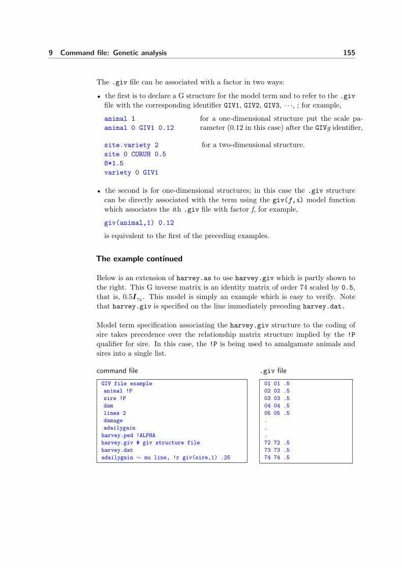
9 Command file: Genetic analysis 155

The .giv file can be associated with a factor in two ways:

• the first is to declare a G structure for the model term and to refer to the .givfile with the corresponding identifier GIV1, GIV2, GIV3, · · ·, ; for example,

animal 1animal 0 GIV1 0.12

for a one-dimensional structure put the scale pa-rameter (0.12 in this case) after the GIVg identifier,

site.variety 2site 0 CORUH 0.58*1.5variety 0 GIV1

for a two-dimensional structure.

• the second is for one-dimensional structures; in this case the .giv structurecan be directly associated with the term using the giv(f,i) model functionwhich associates the ith .giv file with factor f, for example,

giv(animal,1) 0.12

is equivalent to the first of the preceding examples.

The example continued

Below is an extension of harvey.as to use harvey.giv which is partly shown tothe right. This G inverse matrix is an identity matrix of order 74 scaled by 0.5,that is, 0.5I74 . This model is simply an example which is easy to verify. Notethat harvey.giv is specified on the line immediately preceding harvey.dat.

Model term specification associating the harvey.giv structure to the coding ofsire takes precedence over the relationship matrix structure implied by the !Pqualifier for sire. In this case, the !P is being used to amalgamate animals andsires into a single list.

command file .giv file

GIV file example

animal !P

sire !P

dam

lines 2

damage

adailygain

harvey.ped !ALPHA

harvey.giv # giv structure file

harvey.dat

adailygain ∼ mu line, !r giv(sire,1) .25

01 01 .5

02 02 .5

03 03 .5

04 04 .5

05 05 .5

.

.

.

72 72 .5

73 73 .5

74 74 .5

10 Tabulation of the data andprediction from the model

Introduction

Tabulation

Prediction

Underlying principles

Syntax

Examples

156

10 Tabulation of the data and prediction from the model 157

10.1 Introduction

This chapter describes the tabulate directive and the predict directive intro-duced in Section 3.4 under Prediction.

Tabulation is the process of forming simple tables of averages and counts fromthe data. Such tables are useful for looking at the structure of the data andnumbers of observations associated with factor combinations. Multiple tabulatedirectives may be specified in a job.

Prediction is the process of forming a linear function of the vector of fixed andrandom effects in the linear model to obtain an estimated or predicted value for aquantity of interest. It is primarily used for predicting tables of adjusted means.If a table is based on a subset of the explanatory variables then the other variablesneed to be accounted for. It is usual to form a predicted value either at specifiedvalues of the remaining variables, or averaging over them in some way.

10.2 Tabulation

A tabulate directive is provided to enable simple summaries of the data to beformed for the purpose of checking the structure of the data. The summaries arebased on the same records as are used in the analysis of the model (i.e. leavingout records eliminated from the analysis because of missing values in variatesand factors in the model). Multiple tabulate statements are permitted eitherimmediately before or after the linear model. If a linear (mixed) model is notNew

supplied, tabulation is based on all records.

The tabulate statement has the form

tabulate response variables [!WT weight !COUNT !DECIMALS [d] !SD !RANGE!STATS !FILTER filter !SELECT value] ∼ factors

• tabulate is the directive name and must begin in column 1,

• response variables is a list of variates for which means are required,

• !WT weight nominates a variable containing weights,

• !COUNT requests counts as well as means to be reported,

• !DECIMALS [d] (1 ≤ d ≤ 7) requests means be reported with d decimal places. IfNew

omitted, ASReml reports 5 significant digits; if specified without an argument,2 decimal places are reported,

10 Tabulation of the data and prediction from the model 158

• !RANGE requests the minimum and maximum of each cell be reported,

• !SD requests the standard deviation within each cell be reported,

• !STATS is shorthand for !COUNT !SD !RANGE,New

• !FILTER filter nominates a factor for selecting a portion of the data,

• !SELECT value indicates that only records with value in the filter column areto be included,

• ∼ factors identifies the factors to be used for classifying the data. Only factors(not covariates) may be nominated and no more than six may be nominated.

ASReml prints the multiway table of means omitting empty cells to a file withextension .tab.

10.3 Prediction

Underlying principles

Our approach to prediction is a generalization of that of Lane and Nelder (1982)who consider fixed effects models. They form fitted values for all combinationsof the explanatory variables in the model, then take marginal means across theexplanatory variables not relevent to the current prediction. Our case is moregeneral in that random effects can be fitted in our (mixed) models. A full de-scription can be found in Gilmour et al. (2004) and Welham et al. (2004).

Random factor terms may contribute to predictions in several ways. They maybe evaluated at values specified by the user, they may be averaged over, or theymay be omitted from the fitted values used to form the prediction. Averagingover the set of random effects gives a prediction specific to the random effectsobserved. We call this a ‘conditional’ prediction. Omitting the term from themodel produces a prediction at the population average (zero), that is, substitutingthe assumed population mean for an unknown random effect. We call this a‘marginal’ prediction. Note that in any prediction, some terms may be evaluatedas conditional and others at marginal values, depending on the aim of prediction.

For fixed factors there is no pre-defined population average, so there is no naturalinterpretation for a prediction derived by omitting a fixed term from the fittedvalues. Averages must therefore be taken over all the levels present to give asample specific average, or prediction must be at specified levels.

10 Tabulation of the data and prediction from the model 159

For covariate terms (fixed or random) the associated effect represents the coef-ficient of a linear trend in the data with respect to the covariate values. Theseterms should be evaluated at a given value of the covariate, or averaged over sev-eral given values. Omission of a covariate from the predictive model is equivalentto predicting at a zero covariate value, which is often inappropriate.

Interaction terms constructed from factors generate an effect for each combinationof the factor levels, and behave like single factor terms in prediction. Interactionsconstructed from covariates fit a linear trend for the product of the covariatevalues and behave like a single covariate term. An interaction of a factor and acovariate fits a linear trend for the covariate for each level of the factor. For bothfixed and random terms, a value for the covariate must be given, but the factormay be evaluated at a given level, averaged over or (for random terms) omitted.

Before considering some examples in detail, it is useful to consider the conceptualsteps involved in the prediction process. Given the explanatory variables used todefine the linear (mixed) model, the four main steps are

(a) Choose the explanatory variable(s) and their respective value(s) for whichpredictions are required; the variables involved will be referred to as the classifyset and together define the multiway table to be predicted.

(b) Determine which variables should be averaged over to form predictions. Thevalues to be averaged over must also be defined for each variable; the variablesinvolved will be referred to as the averaging set. The combination of the classifyset with these averaging variables defines a multiway hyper-table. Note thatvariables evaluated at only one value, for example, a covariate at its mean value,can be formally introduced as part of the classifying or averaging set.

(c) Determine which terms from the linear mixed model are to be used in formingpredictions for each cell in the multiway hyper-table in order to give appropriateconditional or marginal prediction.

(d) Choose the weights to be used when averaging cells in the hyper-table toproduce the multiway table to be reported.

Note that after steps (a) and (b) there may be some explanatory variables in thefitted model that do not classify the hyper-table. These variables occur in termsthat are ignored when forming the predicted values. It was concluded above thatfixed terms could not sensibly be ignored in forming predictions, so that variables

10 Tabulation of the data and prediction from the model 160

should only be omitted from the hyper-table when they only appear in randomterms. Whether terms derived from these variables should be used when formingpredictions depends on the application and aim of prediction.

The main difference in this prediction process compared to that described by Laneand Nelder (1982) is the choice of whether to include or exclude model terms whenforming predictions. In linear models, since all terms are fixed, terms not in theclassify set must be in the averaging set.

Predict syntax

NIN Alliance trial 1989

variety !A...

column 11

nin89.asd !skip 1

yield ∼ mu variety !r repl

predict variety

0 0 1

repl 1

repl 0 IDV 0.1

The first step is to specify the classify set ofexplanatory variables after the predict direc-tive. The predict statement(s) may appearimmediately after the model line (before or af-ter any tabulate statements) or after the Rand G structure lines. The syntax is

predict factors [qualifiers]

• predict must be the first element of thepredict statement, commencing in column 1 in upper or lower case,

• factors is a list of the variables defining a multiway table to be predicted; eachvariable may be followed by a list of specific values to be predicted,

• the qualifiers, listed in Table 10.1, instruct ASReml to modify the predictionsin some way,

• a predict statement may be continued on subsequent lines by terminating thecurrent line with a comma,

• several predict statements may be specified.

ASReml parses the predict statement before fitting the model. If any syntaxproblems are encountered, these are reported in the .pvs file after which thestatement is ignored: the job is completed as if the erroneous prediction statementdid not exist. The predictions are formed as an extra process in the final iterationand are reported to the .pvs file. Consequently, aborting a run by creating theABORTASR.NOW file (see page 65) will cause any predict statements to be ignored.

By default, factors are predicted at each level, simple covariates are predictedat their overall mean and covariates used as a basis for splines or orthogonal

10 Tabulation of the data and prediction from the model 161

polynomials are predicted at their design points. Covariates grouped into a singleterm (using !G qualifier page 49) are treated as covariates.

Model terms mv and units are always ignored.

Prediction at particular values of a covariate or particular levels of a factor isachieved by listing the values after the variate/factor name. Where there is asequence of values, use the notation a b ... n to represent the sequence of valuesfrom a to n with step size b − a. The default stepsize is 1 (in which case b maybe omitted). A colon (:) may replace the ellipsis (...). An increasing sequenceis assumed. When giving particular values for factors, the default is to use thecoded level (1:n) rather than the label (alphabetical or integer). To use the label,precede it with a quote (").

The second step is to specify the averaging set. The default averaging set isthose explanatory variables involved in fixed effect model terms that are not inthe classifying set. By default variables that only define random model terms areignored. The qualifier !AVERAGE allows these variables to be added to the defaultaveraging set.

The third step is to select the linear model terms to use in prediction. The defaultis that all model terms based entirely on variables in the classifying and averagingsets are used. Two qualifiers allow this default to be modified by adding (!USE) orremoving (!IGNORE) model terms. The qualifier !ONLYUSE explicitly specifies themodel terms to use, ignoring all others. The qualifier !EXCEPT explicitly specifiesthe model terms not to use, including all others. These qualifiers may implicitlymodify the averaging set by including variables defining terms in the predictedmodel not in the classify set. It is sometimes easier to specify the classify set andthe model terms to use and allow ASReml to construct the averaging set.

The fourth step is to choose the weights to use when averaging over dimensionsin the hyper-table. The default is to simply average over the specified levels butthe qualifier !AVERAGE factor weights allows other weights to be specified.

For example,yield ∼ site variety !r site.variety at(site).blockpredict variety

puts variety in the classify set, site in the averaging set and block in the ig-nore set. Consequently, ASReml forms the site×variety hyper-table from modelterms site, variety and site.variety but ignoring all terms in at(site).block,

10 Tabulation of the data and prediction from the model 162

and then forms averages across sites to produce variety predictions.

There are often situations in which the fixed effects design matrix X is not of fullcolumn rank. These can be classified according to the cause of aliasing.

1. linear dependencies among the model terms due to over-parameterisation ofthe model,

2. no data present for some factor combinations so that the corresponding effectscannot be estimated,

3. linear dependencies due to other, usually unexpected, structure in the data.

The first type of aliasing is imposed by the parameterisation chosen and canbe determined from the model. The second type of aliasing can be detectedwhen setting up the design matrix for parameter estimation (which may requirerevision of imposed constraints). The third type can then be detected duringthe absorption of the mixed model equations. Dependencies (aliasing) can bedealt with in several ways and ASReml checks that predictions are of estimablefunctions in the sense defined by Searle (1971, p160) and are invariant to theconstraint method used.

ASReml doesn’t print predictions of non-estimable functions unless the !PRINTALLprediction

problems qualifier is specified. However, using !PRINTALL is rarely a satisfactory solution.Failure to report predicted values normally means that the predict statement isaveraging over some cells of the hyper-table that have no information and there-fore cannot be averaged in a meaningful way. Appropriate use of the !AVERAGEand/or !PRESENT qualifiers will usually resolve the problem. The !PRESENT qual-ifier enables the construction of means by averaging only the estimable cells of thehyper-table. It is reguarly used for nested factors, for example locations nestedin regions.

Table 10.1 is a list of the prediction qualifiers with the following syntax:

• f is an explanatory variable which is a factor,

• t is a list of terms in the fitted model,

• v is a list of explanatory variables.

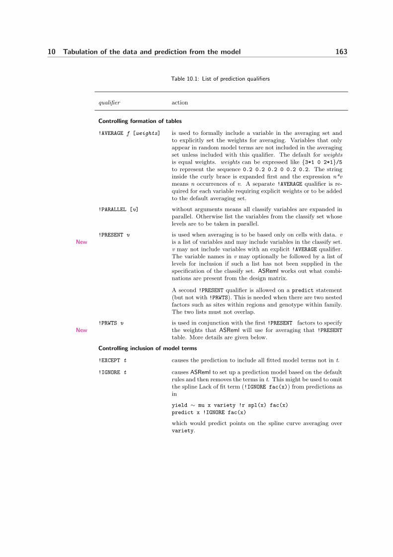
10 Tabulation of the data and prediction from the model 163

Table 10.1: List of prediction qualifiers

qualifier action

Controlling formation of tables

!AVERAGE f [weights] is used to formally include a variable in the averaging set andto explicitly set the weights for averaging. Variables that onlyappear in random model terms are not included in the averagingset unless included with this qualifier. The default for weightsis equal weights. weights can be expressed like 3*1 0 2*1/5to represent the sequence 0.2 0.2 0.2 0 0.2 0.2. The stringinside the curly brace is expanded first and the expression n*vmeans n occurrences of v. A separate !AVERAGE qualifier is re-quired for each variable requiring explicit weights or to be addedto the default averaging set.

!PARALLEL [v] without arguments means all classify variables are expanded inparallel. Otherwise list the variables from the classify set whoselevels are to be taken in parallel.

!PRESENT v

Newis used when averaging is to be based only on cells with data. vis a list of variables and may include variables in the classify set.v may not include variables with an explicit !AVERAGE qualifier.The variable names in v may optionally be followed by a list oflevels for inclusion if such a list has not been supplied in thespecification of the classify set. ASReml works out what combi-nations are present from the design matrix.

A second !PRESENT qualifier is allowed on a predict statement(but not with !PRWTS). This is needed when there are two nestedfactors such as sites within regions and genotype within family.The two lists must not overlap.

!PRWTS v

Newis used in conjunction with the first !PRESENT factors to specifythe weights that ASReml will use for averaging that !PRESENT

table. More details are given below.

Controlling inclusion of model terms

!EXCEPT t causes the prediction to include all fitted model terms not in t.

!IGNORE t causes ASReml to set up a prediction model based on the defaultrules and then removes the terms in t. This might be used to omitthe spline Lack of fit term (!IGNORE fac(x)) from predictions asin

yield ∼ mu x variety !r spl(x) fac(x)

predict x !IGNORE fac(x)

which would predict points on the spline curve averaging overvariety.

10 Tabulation of the data and prediction from the model 164

List of prediction qualifiers

qualifier action

!ONLYUSE t causes the prediction to include only model terms in t. It can beused for example to form a table of slopes as in

HI ∼ mu X variety X.variety

predict variety X 1 !onlyuse X X.variety

!USE t causes ASReml to set up a prediction model based on the defaultrules and then adds the terms listed in t.

Printing

!DEC [n]

Newgives the user control of the number of decimal places reportedin the table of predicted values where n is 0...9. The default is4. G15.9 format is used if n exceeds 9.When !VVP or !SED are used, the values are displayed with 6significant digits unless n is specified and even; then the valuesare displayed with 9 significant digits.

!PLOT [x]

Newinstructs ASReml to attempt a plot of the predicted values. Thisqualifier is only applicable in versions of ASReml linked with theWinteracter Graphics library. If there is no argument, ASRemlproduces a figure of the predicted values as best it can. The usercan modify the appearance by typing <Esc> to expose a menuor with the plot arguments listed in Table 10.2.

!PRINTALL instructs ASReml to print the predicted value, even if it is notof an estimable function. By default, ASReml only prints predic-tions that are of estimable functions.

!SED requests all standard errors of difference be printed. Normallyonly an average value is printed.

!TDIFF requests t-statistics be printed for all combinations of predictedvalues.

!TURNINGPOINTS nrequests ASReml to scan the predicted values from a fitted linefor possible turning points and if found, report them and savethem internally in a vector which can be accessed by subsequentparts of the same job using $TPn. This was added to facilitatelocation of putative QTL.

!TWOSTAGEWEIGHTS

Newis intended for use with variety trials which will subsequently becombined in a meta analysis. It forms the variance matrix forthe predictions, inverts it and writes the predicted variety meanswith the corresponding diagonal elements of this matrix to the.pvs file. These values are used in some variety testing programsin Australia for a subsequent second stage analysis across manytrials. A data base is used to collect the results from the indi-vidual trials and write out the combined data set. The diagonalelements are used as weights in the combined analysis.

10 Tabulation of the data and prediction from the model 165

List of prediction qualifiers

qualifier action

!VPV requests that the variance matrix of predicted values be printedto the .pvs file.

PLOT graphic control qualifiers

This functionality was developed and this section was written by Damian Collins.

The !PLOT qualifier produces a graphic of the predictions. Where there is moreNew

than one prediction factor, a multi-panel ’trellis’ arrangement may be used. Al-ternatively, one or more factors can be superimposed on the one panel. The datacan be added to the plot to assist informal examination of the model fit.

With no plot options, ASReml chooses an arrangement for plotting the predic-tions by recognising any covariates and noting the size of factors. However, theuser is able to customize how the predictions are plotted by either using optionsto the !PLOT qualifier or by using the graphical interface. The graphical interfaceis accessed by typing Esc when the figure is displayed.

The !PLOT qualifier has the following options:

Table 10.2: List of predict plot options

option action

Lines and data

ˆaddData superimposes the raw data.

ˆaddlabels factors superimposes the raw data with the data points labelled using thegiven factors (which must not be prediction factors). This optionmay be useful to identify individual data points on the graph – forinstance, potential outliers – or alternatively, to identify groupsof data points (e.g. all data points in the same stratum).

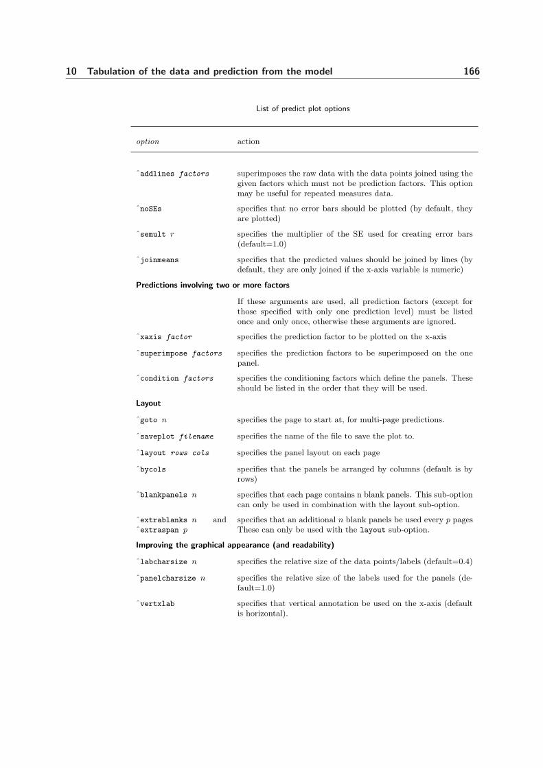
10 Tabulation of the data and prediction from the model 166

List of predict plot options

option action

ˆaddlines factors superimposes the raw data with the data points joined using thegiven factors which must not be prediction factors. This optionmay be useful for repeated measures data.

ˆnoSEs specifies that no error bars should be plotted (by default, theyare plotted)

ˆsemult r specifies the multiplier of the SE used for creating error bars(default=1.0)

ˆjoinmeans specifies that the predicted values should be joined by lines (bydefault, they are only joined if the x-axis variable is numeric)

Predictions involving two or more factors

If these arguments are used, all prediction factors (except forthose specified with only one prediction level) must be listedonce and only once, otherwise these arguments are ignored.

ˆxaxis factor specifies the prediction factor to be plotted on the x-axis

ˆsuperimpose factors specifies the prediction factors to be superimposed on the onepanel.

ˆcondition factors specifies the conditioning factors which define the panels. Theseshould be listed in the order that they will be used.

Layout

ˆgoto n specifies the page to start at, for multi-page predictions.

ˆsaveplot filename specifies the name of the file to save the plot to.

ˆlayout rows cols specifies the panel layout on each page

ˆbycols specifies that the panels be arranged by columns (default is byrows)

ˆblankpanels n specifies that each page contains n blank panels. This sub-optioncan only be used in combination with the layout sub-option.

ˆextrablanks n andˆextraspan p

specifies that an additional n blank panels be used every p pagesThese can only be used with the layout sub-option.

Improving the graphical appearance (and readability)

ˆlabcharsize n specifies the relative size of the data points/labels (default=0.4)

ˆpanelcharsize n specifies the relative size of the labels used for the panels (de-fault=1.0)

ˆvertxlab specifies that vertical annotation be used on the x-axis (defaultis horizontal).

10 Tabulation of the data and prediction from the model 167

List of predict plot options

option action

ˆabbrdlab n specifies that the labels used for the data be abbreviated to ncharacters.

ˆabbrxlab n specifies that the labels used for the x-axis annotation be appre-viated to n characters.

ˆabbrslab n specifies that the labels used for superimposed factors be abbre-viated to n characters.

Complicated weighting

Generally, when forming a prediction table, it is necessary to average over (orNew

ignore) some potential dimensions of the prediction table. By default, ASReml

uses equal weights (1/f for a factor with f levels). More complicated weightingis achieved by using the !AVERAGE qualifier to set specific (unequal) weights foreach level of a factor. However, sometimes the weights to be used need to bedefined with respect to two or more factors. The simplest case is when there aremissing cells and weighting is equal for those cells in a multiway table that arepresent; achieved by using the !PRESENT qualifier. This is now further generalizedby allowing the user to fill in the weights for use by the !PRESENT machinery viathe !PRWTS qualifier.

The user specifies the factors in the table of weights with the !PRESENT statementand then gives the table of weights using the !PRWTS qualifier. There may only beone !PRESENT qualifier on the predict line when !PRWTS is specified. The orderof factors in the tables of weights must correspond to the order in the !PRESENTlist with later factors nested within preceding factors. Check the output to ensureCaution

that the values in the tables of weights are applied in the correct order. ASReml

may transpose the table of weights to match the order it needs for processing.

Consider a rather complicated example from a rotation experiment conductedover several years. This particular analysis followed the analysis of the daily liveweight gain per hectare of the sheep grazing the plots. There were periods whenno sheep grazed. Different flocks grazed in the different years. Daily liveweight

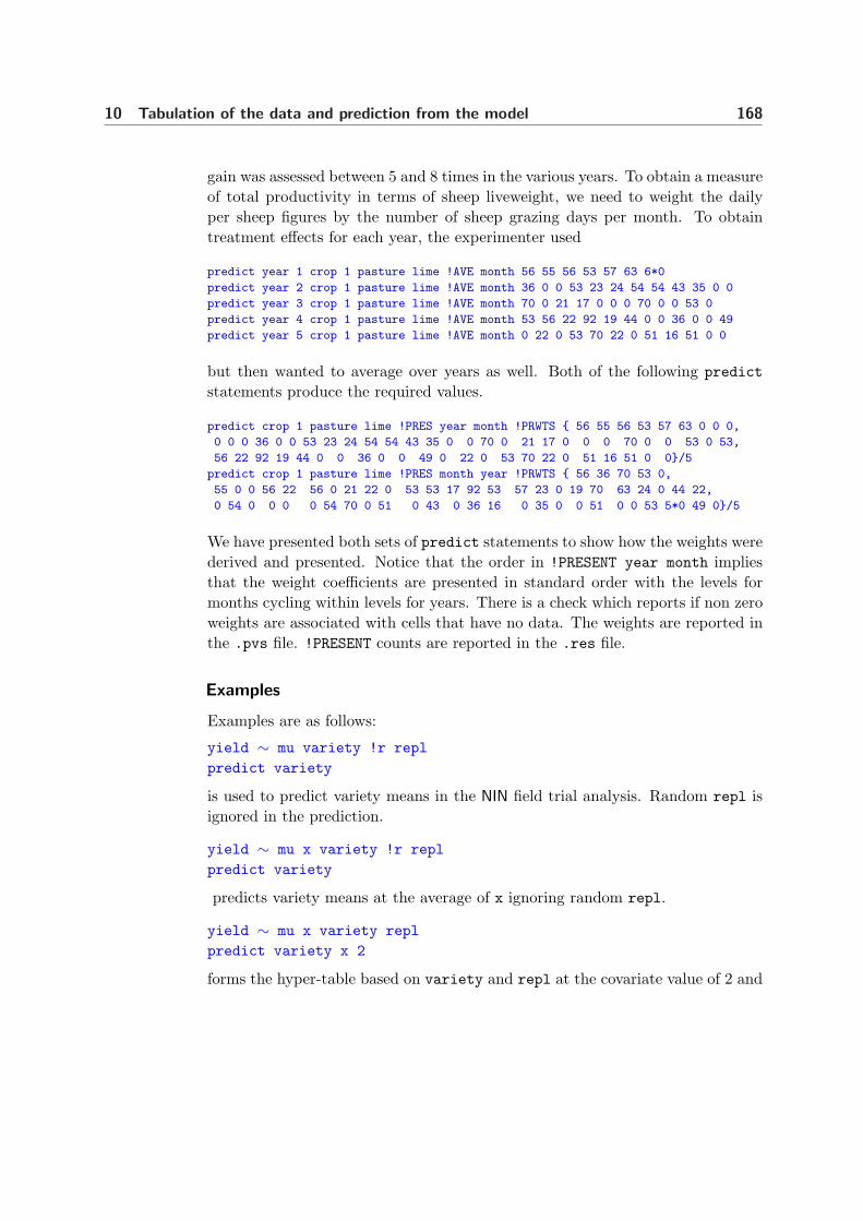
10 Tabulation of the data and prediction from the model 168

gain was assessed between 5 and 8 times in the various years. To obtain a measureof total productivity in terms of sheep liveweight, we need to weight the dailyper sheep figures by the number of sheep grazing days per month. To obtaintreatment effects for each year, the experimenter used

predict year 1 crop 1 pasture lime !AVE month 56 55 56 53 57 63 6*0

predict year 2 crop 1 pasture lime !AVE month 36 0 0 53 23 24 54 54 43 35 0 0

predict year 3 crop 1 pasture lime !AVE month 70 0 21 17 0 0 0 70 0 0 53 0

predict year 4 crop 1 pasture lime !AVE month 53 56 22 92 19 44 0 0 36 0 0 49

predict year 5 crop 1 pasture lime !AVE month 0 22 0 53 70 22 0 51 16 51 0 0

but then wanted to average over years as well. Both of the following predictstatements produce the required values.

predict crop 1 pasture lime !PRES year month !PRWTS 56 55 56 53 57 63 0 0 0,

0 0 0 36 0 0 53 23 24 54 54 43 35 0 0 70 0 21 17 0 0 0 70 0 0 53 0 53,

56 22 92 19 44 0 0 36 0 0 49 0 22 0 53 70 22 0 51 16 51 0 0/5

predict crop 1 pasture lime !PRES month year !PRWTS 56 36 70 53 0,

55 0 0 56 22 56 0 21 22 0 53 53 17 92 53 57 23 0 19 70 63 24 0 44 22,

0 54 0 0 0 0 54 70 0 51 0 43 0 36 16 0 35 0 0 51 0 0 53 5*0 49 0/5

We have presented both sets of predict statements to show how the weights werederived and presented. Notice that the order in !PRESENT year month impliesthat the weight coefficients are presented in standard order with the levels formonths cycling within levels for years. There is a check which reports if non zeroweights are associated with cells that have no data. The weights are reported inthe .pvs file. !PRESENT counts are reported in the .res file.

Examples

Examples are as follows:

yield ∼ mu variety !r replpredict variety

is used to predict variety means in the NIN field trial analysis. Random repl isignored in the prediction.

yield ∼ mu x variety !r replpredict variety

predicts variety means at the average of x ignoring random repl.

yield ∼ mu x variety replpredict variety x 2

forms the hyper-table based on variety and repl at the covariate value of 2 and

10 Tabulation of the data and prediction from the model 169

then averages across repl to produce variety predictions.

GFW Fdiam ∼ Trait Trait.Year !r Trait.Teampredict Trait Team

forms the hyper-table for each trait based on Year and Team with each linearcombination in each cell of the hyper-table for each trait using Team and Yeareffects. Team predictions are produced by averaging over years.

yield ∼ variety !r site.varietypredict variety

will ignore the site.variety term in forming the predictions while

predict variety !AVERAGE site

forms the hyper-table based on site and variety with each linear combinationin each cell using variety and site.variety effects and then forms averagesacross sites to produce variety predictions.

yield ∼ site variety !r site.variety at(site).blockpredict variety

puts variety in the classify set, site in the averaging set and block in the ignoreset. Consequently, it forms the site×variety hyper-table from model termssite, variety and site.variety but ignoring all terms in at(site).block,and then forms averages across sites to produce variety predictions.

11 Functions of variancecomponents

Introduction

Syntax

Linear combinations of componentsHeritabilityCorrelation

A more detailed example

170

11 Functions of variance components 171

11.1 Introduction

F phenvar 1 + 2 # pheno var

F genvar 1 * 4 # geno var

H herit 4 3 # heritability

ASReml includes a post-analysis procedure tocalculate functions of variance components.Its intended use is when the variance compo-nents are either simple variances or are vari-ances and covariances in an unstructured matrix. The functions covered are linearcombinations of the variance components (for example, phenotypic variance), aratio of two components (for example, heritabilities) and the correlation basedon three components (for example, genetic correlation). The user must preparea .pin file. A simple sample .pin file is shown in the ASReml code box above.The .pin file specifies the functions to be calculated. The user re-runs ASReml

with the -P command line option specifying the .pin file as the input file. AS-

Reml reads the model information from the .asr and .vvp files and calculatesthe requested functions. These are reported in the .pvc file.

11.2 Syntax

Functions of the variance components are specified in the .pin file in lines of theformletter label coefficients

• letter ( either F, H or R ) must occur in column 1

– F is for linear combinations of variance components,– H is for forming the ratio of two components,– R is for forming the correlation based on three components,

• label names the result,

• coefficients is the list of coefficients for the linear function.

Linear combinations of components

F phenvar 1 + 2 # pheno var

F genvar 1 * 4 # geno var

H herit 4 3 # heritability

First ASReml extracts the variance compo-nents from the .asr file and their variancematrix from the .vvp file. Each linear func-tion formed by an F line is added to the list ofcomponents. Thus, the number of coefficients increases by one each line. We seekto calculate k + c′v, cov (c′v, v) and var (c′v) where v is the vector of existingvariance components, c is the vector of coefficients for the linear function andk is an optional offset which is usually omitted but would be 1 to represent the

11 Functions of variance components 172

residual variance in a probit analysis and 3.289 to represent the residual variancein a logit analysis. The general form of the directive is

F label a + b ∗ cb + c + d + m ∗ k

where a, b, c and d are subscripts to existing components va, vb, vc and vd andcb is a multiplier for vb. m is a number bigger than the current length of v to flagthe special case of adding the offset k. Where matrices are to be combined theform

F label a:b * k + c:d

can be used, as in the Coopworth data example, see page 300.

Assuming that the .pin file in the ASReml code box corresponds to a simple siremodel and that variance component 1 is the sire variance and variance component2 is the residual variance, then

F phenvar 1 + 2

gives a third component which is the sum of the variance components, that is,the phenotypic variance, and

F genvar 1 * 4

gives a fourth component which is the sire variance component multiplied by 4,that is, the genotypic variance.

Heritability

F phenvar 1 + 2 # pheno var

F genvar 1 * 4 # geno var

H herit 4 3 # heritability

Heritabilities are requested by lines in the.pin file beginning with an H. The specificform of the directive in this case is

H label n d

This calculates σ2n/σ2

d and se[σ2n/σ2

d] where n and d are integers pointing to com-ponents vn and vd that are to be used as the numerator and denominator respec-tively in the heritability calculation.

Var(σ2n

σ2d) = (σ2

n

σ2d)2(Var(σ2

n)σ4

n+ Var(σ2

d)

σ4d

− 2Cov(σ2n,σ2

d)

σ2nσ2

d)

In the example

H herit 4 3

calculates the heritability by calculating component 4 (from second line of .pin)

11 Functions of variance components 173

/ component 3 (from first line of .pin), that is, genetic variance / phenotypicvariance.

Correlation

F phenvar 1:3 + 4:6

R phencorr 7 8 9

R gencorr 4:6

Correlations are requested by lines in the .pinfile beginning with an R. The specific form ofthe directive is

R label a ab b

This calculates the correlation r = σab/√

σ2aσ

2b and the associated standard error.

a, b and ab are integers indicating the position of the components to be used.Alternatively,

R label a:n

calculates the correlation r = σab/√

σ2aσ

2b for all correlations in the lower tri-

angular row-wise matrix represented by components a to n and the associatedstandard errors.

var (r) = r2[var

(σ2

a

)

4σ2a2 +

var(σ2

b

)

4σ2b2 +

var (σab)σ2

ab

+2cov

(σ2

a

)σ2

b

4σ2aσ

2b

− 2cov(σ2

a

)σab

2σ2aσab

− 2cov (σab) σ2b

2σabσ2b

]

In the example

R phencorr 7 8 9

calculates the phenotypic covariance by calculatingcomponent 8 /

√component 7 × component 9 where components 7, 8 and 9 are

created with the first line of the .pin file, and

R gencorr 4:6

calculates the genotypic covariance by calculatingcomponent 5 /

√component 4 × component 6 where components 4, 5 and 6 are

variance components from the analysis.

11 Functions of variance components 174

A more detailed example

For convenience in preparing the .pin file, some users copy the variance compo-nent lines from the .asr file and insert them at the top of the .pin file, beingcareful to retain one leading space so that the lines will be just copied and oth-erwise ignored as the .pin file is processed.

Bivariate sire model

sire !I

ywt fat

bsiremod.asd

ywt fat ∼ Trait !r Trait.sire

1 2 1

0 # ASReml will count units

Trait 0 US

3*0

Trait.sire 2

Trait 0 US

3*0

sire

The following sample .pin file is a little morecomplicated. It relates to the bivariate siremodel in bsiremod.as shown in the code boxto the right.

The first six lines of the .pin file contain thevariance component table on which the .pinfile is based, copied from the the .asr file forconverience in coding the rest of the file.

Residual UnStruct 1 26.2197 26.2197 18.01 0 U

Residual UnStruct 1 2.85090 2.85090 9.55 0 U

Residual UnStruct 2 1.71556 1.71556 18.00 0 U

Tr.sire UnStruct 1 16.5262 16.5262 2.69 0 U

Tr.sire UnStruct 1 1.14422 1.14422 1.94 0 U

Tr.sire UnStruct 2 0.132847 0.132847 1.88 0 U

F phenvar 1:3 + 4:6

F addvar 4:6 * 4

H heritA 10 7

H heritB 12 9

R phencorr 7 8 9

R gencor 4:6

Numbering the parameters reported in bsiremod.asr (andbsiremod.vvp)

123456

error variance for ywterror covariance for ywt and faterror variance for fatsire variance component for ywtsire covariance for ywt and fatsire variance for fat

then

11 Functions of variance components 175

F phenvar 1:3 + 4:6

creates new components 7 = 1+4, 8 = 2+5 and 9 = 3+6,

F addvar 4:6 * 4

creates new components 10 = 4 × 4, 11 = 5 × 4 and 12 = 6 × 4,

H heritA 10 7

forms 10 / 7 to give the heritability for ywt,

H heritB 12 9

forms 12 / 9 to give the heritability for fat,

R phencorr 7 8 9

forms 8 /√

7 × 9, that is, the phenotypic correlation between ywt and fat,

R gencorr 4:6

forms 5 /√

4×6, that is, the genetic correlation between ywt and fat.

The result is:7 phenvar 1 42.75 6.297.pvc file

8 phenvar 2 3.995 0.6761

9 phenvar 3 1.848 0.1183

10 addvar 4 66.10 24.58

11 addvar 5 4.577 2.354

12 addvar 6 0.5314 0.2831

h2ywt = addvar 10/phenvar 7= 1.5465 0.3574

h2fat = addvar 12/phenvar 9= 0.2875 0.1430

phencorr = phenvar /SQR[phenvar *phenvar ]= 0.4495 0.0483

gencor 2 1 = Tr.si 5/SQR[Tr.si 4*Tr.si 6]= 0.7722 0.1537

12 Command file: Running the job

Introduction

The command line

Normal runProcessing a .pin file

Forming a job template

Command line options

Prompt for argumentsOutput control command line options

Debug command line optionsGraphics command line options

Job control command line optionsWorkspace command line options

Menu command line optionsNon-graphics command line options

Examples

Advanced processing arguments

Standard use of argumentsPrompting for input

Paths and Loops

176

12 Command file: Running the job 177

12.1 Introduction

The command line, its options and arguments are discussed in this chapter. Com-mand line options enable more workspace to be accessed to run the job, controlsome graphics output and control advanced processing options. Command linearguments are substituted into the job at run time.

As Windows likes to hide the command line, most command line options can beset on an optional initial line of the .as file we call the top job control line todistinguish it from the other job control lines discussed in Chapter 6. If the firstline of the .as file contains a qualifier other than !DOPATH, it is interpreted assetting command line options and the Title is taken as the next line.

12.2 The command line

Normal run

The basic command to run ASReml is

[path]ASReml basename[.as[c]]

• path provides the path to the ASReml program (usually called asreml.exe ina PC environment). In a UNIX environment, ASReml is usually run through ashell script called ASReml.

– if the ASReml program is in the search path then path is not required andthe word ASReml will suffice; for example

ASReml nin89.as

will run the NIN analysis,– if asreml.exe(ASReml) is not in the search path then path is required, for

example, if asreml.exe is in the usual place then

c:\Program Files\ASReml2\bin\Asreml nin89.as

will run nin89.as,

• ASReml invokes the ASReml program,

• basename is the name of the .as[c] command file.

The basic command line can be extended with options and arguments to

[path] ASReml [options] basename[.as[c]] [arguments]

12 Command file: Running the job 178

• options is a string preceded by a - (minus) sign. Its components control severaloperations (batch, graphic, workspace, . . . ) at run time; for example, thecommand line

ASReml -w128 rat.as

tells ASReml to run the job rat.as with workspace allocation of 128mb,

• arguments provide a mechanism (mostly for advanced users) to modify a jobat run time; for example, the command line

ASReml rat.as alpha beta

tells ASReml to process the job in rat.as as if it read alpha wherever $1 ap-pears in the file rat.as, beta wherever $2 appears and 0 wherever $3 appears(see below).

Processing a .pin file

If the filename argument is a .pin file, (see Chapter 11), then ASReml processesit. If the pinfile basename differs from the basename of the output files it isprocessing, then the basename of the output files must be specified with the Poption letter. Thus

ASReml border.pin

will perform the pinfile calculations defined in border.pin on the results in filesborder.asr and border.vvp.

ASReml -Pborderwwt border.pin

will perform the pinfile calculations defined in border.pin on the results in filesborderwwt.asr and borderwwt.vvp.

Forming a job template from data file

The facility to generate a template .as file has been moved to the command line,and extended. Normally, the name of a .as command file is specified on thecommand line. If a .as file does not exist and a file with file extension .asd,New

.csv, .dat, .gsh, .txt or .xls is specified, ASReml assumes the data file has fieldlabels in the first row and generates a .as file template. First, it seeks to convertthe .gsh (Genstat) or .xls (Excel, see page 44) file to .csv format using theASRemload.dll utility provided by VSN. In generating the .as template, ASReml

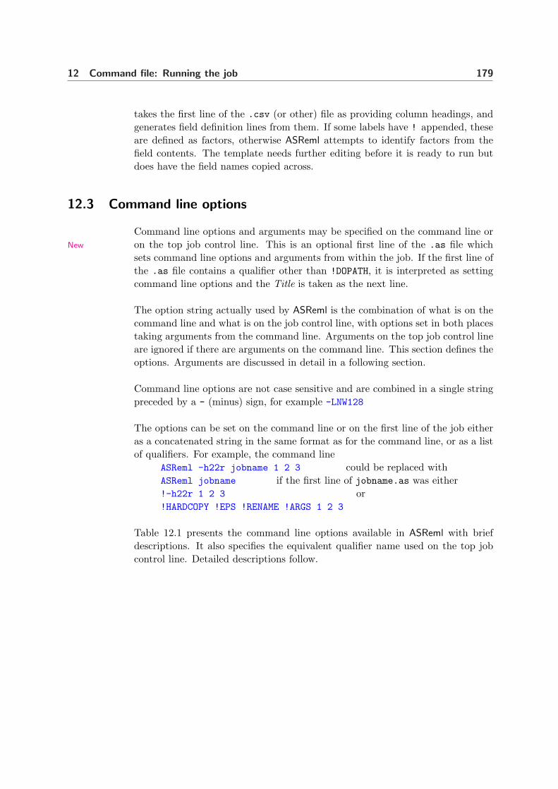
12 Command file: Running the job 179

takes the first line of the .csv (or other) file as providing column headings, andgenerates field definition lines from them. If some labels have ! appended, theseare defined as factors, otherwise ASReml attempts to identify factors from thefield contents. The template needs further editing before it is ready to run butdoes have the field names copied across.

12.3 Command line options

Command line options and arguments may be specified on the command line oron the top job control line. This is an optional first line of the .as file whichNew

sets command line options and arguments from within the job. If the first line ofthe .as file contains a qualifier other than !DOPATH, it is interpreted as settingcommand line options and the Title is taken as the next line.

The option string actually used by ASReml is the combination of what is on thecommand line and what is on the job control line, with options set in both placestaking arguments from the command line. Arguments on the top job control lineare ignored if there are arguments on the command line. This section defines theoptions. Arguments are discussed in detail in a following section.

Command line options are not case sensitive and are combined in a single stringpreceded by a - (minus) sign, for example -LNW128

The options can be set on the command line or on the first line of the job eitheras a concatenated string in the same format as for the command line, or as a listof qualifiers. For example, the command line

ASReml -h22r jobname 1 2 3 could be replaced withASReml jobname if the first line of jobname.as was either!-h22r 1 2 3 or!HARDCOPY !EPS !RENAME !ARGS 1 2 3

Table 12.1 presents the command line options available in ASReml with briefdescriptions. It also specifies the equivalent qualifier name used on the top jobcontrol line. Detailed descriptions follow.

12 Command file: Running the job 180

Table 12.1: Command line options

option qualifier type action

Frequently used command line options

C !CONTINUE job control continue iterations using previous esti-mates as initial values

F !FINAL job control continue for one more iteration usingprevious estimates as initial values

L !LOGFILE screen output copy screen output to basename.asl

N !NOGRAPHS graphics suppress interactive graphics

Ww !WORKSPACE w workspace set workspace size to w Mbyte

Other command line options

!ARGS a job control to set arguments (a) in job rather thanon command line

A !ASK job control prompt for options and arguments

Bb !BRIEF b output control reduce output to .asr file

D !DEBUG debug invoke debug mode

E !DEBUG 2 debug invoke extended debug mode

Gg !GRAPHICS g graphics set interactive graphics device

Hg !HARDCOPY g graphics set interactive graphics device,graphics screens not displayed

I !INTERACTIVE graphics display graphics screen

J !JOIN output control concatenate !CYCLE output files

O !ONERUN job control override rerunning requested by!RENAME

P NA post-processing calculation of functions of variancecomponents

Q !QUIET graphics suppress screen output

Rr !RENAME job control repeat run for each argument renamingoutput filenames

Ss NA workspace set workspace size

Yv !YVAR v job control over-ride y-variate specified in the com-mand file with variate number v

Z NA license reports current license details

12 Command file: Running the job 181

Prompt for arguments (A)

A (!ASK) makes it easier to specify command line options in Windows Explorer.One of the options available when right clicking a .as file, invokes ASReml withthis option. ASReml then prompts for the options and arguments, allowing theseto be set interactively at run time. With !ASK on the top job control line, it isassumed that no other qualifiers are set on the line. For example, a response of

-h22r 1 2 3 would be equivalent toASReml -h22r basename 1 2 3

Output control (B, J)

B[b] (!BRIEF [b) suppresses some of the information written to the .asr file. TheNew

data summary and regression coefficient estimates are suppressed by the optionsB, B1 or B2. This option should not be used for initial runs of a job before youhave confirmed (by checking the data summary) that ASReml has read the dataas you intended. Use B2 to also have the predicted values written to the .asr fileinstead of the .pvs file. Use B-1 to get BLUE estimates reported in .asr file.

J (!JOIN) is used in association with the !CYCLE qualifier to put the outputNew

from a set of runs into single files (see !CYCLE list !JOIN on page 186).

Debug command line options (D, E)

D and E (!DEBUG, !DEBUG 2) invoke debug mode and increase the informationwritten to the screen or .asl file. This information is not useful to most users.On Unix systems, if ASReml is crashing use the system script command tocapture the screen output rather than using the L option, as the .asl file is notproperly closed after a crash.

Graphics command line options (G, H, I, N, Q)

Graphics are produced in the PC, Linux and SUN 32bit versions of ASReml usingthe Winteracter graphics library.

The I (!INTERACTIVE) option permits the variogram and residual graphics to bedisplayed. This is the default unless the L option is specified.

The N (!NOGRAPHICS) option prevents any graphics from being displayed. Thisis also the default when the L option is specified.

The Gg (!GRAPHICS g) option sets the file type for hard copy versions of thegraphics. Hard copy is formed for all the graphics that are displayed.

12 Command file: Running the job 182

H[g] (!HARDCOPY g) replaces the G option when graphics are to be written to fileNew

but not displayed on the screen. The H may be followed by a format code e.g.H22 for .eps.

Q (!QUIET) is used when running under the control of and editor such as ASReml-New

Wto suppress any POPUPs/ PAUSES from ASReml.

ASReml writes the graphics to files whose names are built up as<basename>[<args>]<type>[<pass>][<section>].<ext> where squareparentheses indicate elements that might be omitted, <basename> is the nameportion of the .as file, <args> is any argument strings built into the outputnames by use of the !RENAME qualifier, <type> indicates the contents of the figure(as given in the following table), <pass> is inserted when the job is repeated(!RENAME or !CYCLE) to ensure filenames are unique across repeats, <section> isinserted to distinquish files produced from different sections of data (for examplefrom multisite spatial analysis) and <ext> indicates the file graphics format.

<type> file contents

R marginal means of residuals from spatial analysis of a sectionV variogram of residuals from spatial analysis for a sectionS residuals in field plan for a sectionH histogram of residuals for a sectionRvE residuals plotted against expected valuesXYGi figure produced by !X, !Y and !G qualifiersPV i Predicted values plotted for PREDICT directive i

The graphics file format is specified by following the G or H option by a numberg, or specifying the appropriate qualifier on the top job control line, as follows:

g qualifier description <ext>

1 !HPGL HP-GL pgl2 !PS Postscript (default) ps6 !BMP BMP bmp

10 !WPM Windows Print Manager11 !WMF Windows Meta File wmf12 !HPGL 2 HP-GL2 hgl22 !EPS EncapsulatedPostScript eps

12 Command file: Running the job 183

Job control command line options (C, F, O, R)

C (!CONTINUE) indicates that the job is to continue iterating from the values inthe .rsv file. This is equivalent to setting !CONTINUE on the datafile line, seeTable 5.4 for details.

F (!FINAL) indicates that the job is to continue for one more iteration from thevalues in the .rsv file. This is useful when using predict, see Chapter 10.

O (!ONERUN) is used with the R option to make ASReml perform a single analysisNew

when the R option would otherwise attempt multiple analyses. The R option thenbuilds some arguments into the output file name while other arguments are not.For example

ASReml -nor2 mabphen 2 TWT out(621) out(929)results in one run with output files mabphen2 TWT.*.

R[r] (!RENAME [r]) is used in conjunction with at least r argument(s) and doesNew

two things: it modifies the output filename to include the first r arguments so theoutput is identified by these arguments, and, if there are more than r arguments,the job is rerun moving the extra arguments up to position r (unless !ONERUN (O)is also set). If r is not specified, it is taken as 1.

For exampleASReml -r2 job wwt gfw fd fat

is equivalent to running three jobs:ASReml -r2 job wwt gfw → jobwwt gfw.asrASReml -r2 job wwt fd → jobwwt fd.asrASReml -r2 job wwt fat → jobwwt fat.asr

Yy (!YVAR y) overrides the value of response, the variate to be analysed (seeSection 6.2) with the value y, where y is the number of the data field containingthe trait to be analysed. This facilitates analysis of several traits under the samemodel. The value of y is appended to the basename so that output files are notoverwritten when the next trait is analysed.

Workspace command line options (S, W)

The workspace requirements depend on problem size and may be quite large. Aninitial workspace allocation may be requested on the command line with the Sor W options; if neither is specified, 32Mbyte (4 million double precision words)is allocated.

12 Command file: Running the job 184

Wm (!WORKSPACE m) sets the initial size of the workspace in Mbytes. For exampleNew

W1600 requests 1600 Mbytes of workspace, the maximum typically available underWindows. W2000 is the maximum available on 32bit Unix(Linux) systems. On64bit systems, the argument, if less than 32, is taken as Gbyte.

Alternatively, Ss can be used to set the initial workspace allocation. s is a digit.The workspace allocated is 2s× 8 Mbyte; S3 is 64Mb, S4 is 128Mb, S5 is 256Mb,S6 is 512Mb, S7 is 1024Mb, S8 is 2048Mb, S9 is 4096Mb. This option was inRelease 1.0; the more flexible option, Wm, has been introduced in Release 2.0.The W option is ignored if the S option is also specified.

Otherwise, additional workspace may be requested with the Ss or Wm optionsor the !WORKSPACE m qualifier on the top job control line if not specified onthe control line. If your system cannot provide the requested workspace, therequest will be diminished until it can be satisfied. On multi-user systems, donot unnecessarily request the maximum or other users may complain.

Having started with an initial allocation, if ASReml realises more space is requiredas it is running, it will attempt to restart the job with increased workspace. Ifthe system has already allocated all available memory the job will stop.

Examples

ASReml code action

asreml -LW64 rat.as increase workspace to 64 Mbyte, send screen output torat.asl and suppress interactive graphics

asreml -IL rat.as send screen output to rat.asl but display interactive graph-ics

asreml -N rat.as allow screen output but suppress interactive graphics

asreml -ILW512 rat.as increase workspace to 512 Mbyte , send screen output torat.asl but display interactive graphics

asreml -rs3 coop wwt ywt runs coop.as twice writing results to coopwwt.as andcoopywt.as using 64Mb workspace and substituting wwt andywt for $1 in the two runs.

12 Command file: Running the job 185

12.4 Advanced processing arguments

Standard use of arguments

Command line arguments are intended to facilitate the running of a sequence ofjobs that require small changes to the command file between runs. The outputfile name is modified by the use of this feature if the -R option is specified. Thisuse is demonstrated in the Coopworth example of Section 15.10, see page 297.

Command line arguments are strings listed on the command line after basename,the command file name, or specified on the top job control line after the !ARGSqualifier. These strings are inserted into the command file at run time. Whenthe input routine finds a $n in the command file it substitutes the nth argument(string). n may take the values 1. . .9 to indicate up to 9 strings after the commandfile name. If the argument has 1 character, a trailing blank is attached to thecharacter and inserted into the command file. If no argument exists, a zero isinserted. For example,

asreml rat.as alpha beta

tells ASReml to process the job in rat.as as if it read alpha wherever $1 appearsin the command file, beta wherever $2 appears and 0 wherever $3 appears.

Table 12.2: The use of arguments in ASReml

in command file on command line becomes in ASReml run

abc$1def no argument abc0 def

abc$1def with argument X abcX def

abc$1def with argument XY abcXYdef

abc$1def with argument XYZ abcXYZdef

abc$1 def with argument XX abcXX def

abc$1 def with argument XXX abcXXX def

abc$1 def

(multiple spaces)with argument XXX abcXXX def

12 Command file: Running the job 186

Prompting for input

Another way to gain some interactive control of a job in the PC environment isto insert !?text in the .as file where you want to specify the rest of the line atrun time. ASReml prompts with text and waits for a response which is used tocompete the line. The !? qualifier may be used anywhere in the job and the lineis modified from that point.

Unfortunately the prompt may not appear on the top screen under some windowsWarningoperating systems in which case it may not be obvious that ASReml is waitingfor a keyboard response.

Paths and Loops

ASReml is designed to analyse just one model per run. However, the analysisof a data set typically requires many runs, fitting different models to differenttraits. It is often convenient to have all these runs coded into a single .as fileand control the details from the command line (or top job control line) usingarguments. The highlevel qualifiers !CYCLE and DOPATH enable multiple analysesto be defined and run in one execution of ASReml.

Table 12.3: High level qualifiers

qualifier action

!CYCLE list [!JOIN]

Newis a mechanism whereby ASReml can loop through a seriesof jobs. The !CYCLE qualifier must appear on its own line,starting in character 1. em list is a series of values which aresubstituted into the job wherever the $I string appears. If!JOIN is not specified, the current value from list is built intothe output filenames writing the output to separate files. If!JOIN is specified, the outputs are written to a single file.For example!CYCLE 0.4 0.5 0.6 !JOIN

20 0 mat2 1.9 $I !GPF

would result in three runs and the results would be appendedto a single file.Warning: The !CYCLE mechanism does not work in combina-tion with the !RENAME qualifier used with multiple commandline arguments.

12 Command file: Running the job 187

High level qualifiers

qualifier action

!DOPATH n The qualifiers !DOPART and !PART have been extended in re-lease 2.0 and !DOPATH and !PATH are thought to be more ap-propriate names. Both spellings can be used interchangably.!DOPATH allows several analyses to be coded and run sequen-tially without having to edit the .as file between runs. Whichparticular lines in the .as file are honoured is controlled bythe argument n of the !DOPATH qualifier in conjunction with!PATH (or !PART) statements.

New

The argument (n) is often given as $1 indicating that theactual path to use is specified as the first argument on thecommand line (see Section 12.4). See Sections 15.7 and 15.10for examples. The default value of n is 1.

!DOPATH n can be located anywhere in the job but if placed onthe top job control line, it cannot have the form !DOPATH $1

unless the arguments are on the command line as the !DOPATHqualifier will be parsed before any job arguments on the sameline are parsed.

!PATH pathlist The !PATH (or !PART) control statement may list multiplepath numbers so that the following lines are honoured if anyone of the listed path numbers is active. The !PATH qualifiermust appear at the beginning of its own line after the !DOPATHqualifier. A sequence of path numbers can be written usinga : b notation. For example

mydata.asd !DOPATH 4

!PATH 2 4 6:10

One situation where this might be useful is where it is neces-sary to run simpler models to get reasonable starting valuesfor more complex variance models. The more complex mod-els are specified in later parts and the !CONTINUE commandis used to pick up the previous estimates.

13 Description of output files

Introduction

An example

Key output files

The .asr fileThe .sln fileThe .yht file

Other ASReml output files

The .aov fileThe .res fileThe .vrb fileThe .vvp fileThe .rsv fileThe .dpr fileThe .pvc fileThe .pvs fileThe .tab file

ASReml output objects and where to find them

188

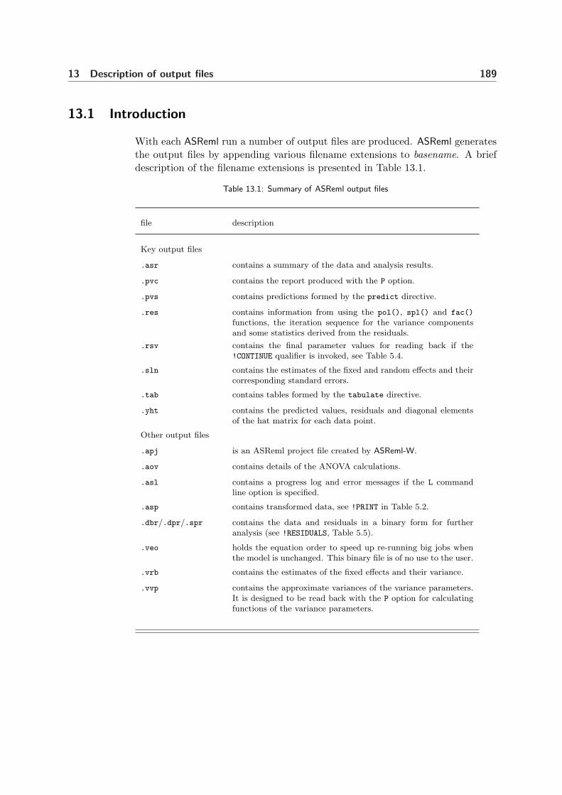
13 Description of output files 189

13.1 Introduction

With each ASReml run a number of output files are produced. ASReml generatesthe output files by appending various filename extensions to basename. A briefdescription of the filename extensions is presented in Table 13.1.

Table 13.1: Summary of ASReml output files

file description

Key output files

.asr contains a summary of the data and analysis results.

.pvc contains the report produced with the P option.

.pvs contains predictions formed by the predict directive.

.res contains information from using the pol(), spl() and fac()

functions, the iteration sequence for the variance componentsand some statistics derived from the residuals.

.rsv contains the final parameter values for reading back if the!CONTINUE qualifier is invoked, see Table 5.4.

.sln contains the estimates of the fixed and random effects and theircorresponding standard errors.

.tab contains tables formed by the tabulate directive.

.yht contains the predicted values, residuals and diagonal elementsof the hat matrix for each data point.

Other output files

.apj is an ASReml project file created by ASReml-W.

.aov contains details of the ANOVA calculations.

.asl contains a progress log and error messages if the L commandline option is specified.

.asp contains transformed data, see !PRINT in Table 5.2.

.dbr/.dpr/.spr contains the data and residuals in a binary form for furtheranalysis (see !RESIDUALS, Table 5.5).

.veo holds the equation order to speed up re-running big jobs whenthe model is unchanged. This binary file is of no use to the user.

.vrb contains the estimates of the fixed effects and their variance.

.vvp contains the approximate variances of the variance parameters.It is designed to be read back with the P option for calculatingfunctions of the variance parameters.

13 Description of output files 190

An ASReml run generates many files and the .sln and .yht files, in particular,are often quite large and could fill up your disk space. You should thereforeregularly tidy your working directories, maybe just keeping the .as, .asr and.pvs files.

13.2 An example

NIN Alliance Trial 1989

variety !A

id

raw

repl 4

nloc

yield

lat

long

row 22

column 11

nin89a.asd !skip 1 !DISPLAY 15

yield ∼ mu variety !f mv

predict variety

1 2 0

row row AR1 0.5

column column AR1 0.5

In this chapter the ASReml output files arediscussed with reference to a two-dimensionalseparable autoregressive spatial analysis of theNIN field trial data, see model 3b on page 111of Chapter 7 for details. The ASReml com-mand file for this analysis is presented to theright. Recall that this model specifies a sep-arable autoregressive correlation structure forresidual or plot errors that is the direct prod-uct of an autoregressive correlation matrix oforder 22 for rows and an autoregressive corre-lation matrix of order 11 for columns. In thiscase 0.5 is the starting correlation for bothcolumns and rows.

13.3 Key output files

The key ASReml output files are the .asr, .sln and .yht files.

The .asr file

This file contains

• a general announcements box (outlined in asterisks) containing current mes-sages,

• a summary of the data to validate the specification of the model,

• a summary of the fitting process to check convergence,

• a summary of the variance parameters:

– The Gamma column reports the actual parameter fitted,– the Component column reports the gamma converted to a variance scale if

appropriate,

13 Description of output files 191

– Comp/SE is the ratio of the component relative to the square root of thediagonal element of the inverse of the average information matrix Warning

Comp/SE should not be used for formal testing,– The % shows the percentage change in the parameter at the last iteration,– use the .pin file described Chapter 11 to calculate meaningful functions of

the variance components,

• an analysis of variance (ANOVA) table (Section 6.12). The table contains thenumerator degrees of freedom for the terms and ’incremental’ F-statistics forapproximate testing of effects. It may also contain denominator degrees offreedon, a ’conditional’ F-statistic and a significance probability.

• estimated effects, their standard errors and t values for equations in the DENSEportion of the SSP matrix are reported if !BRIEF -1 is invoked; the T-prevcolumn tests difference between successive coefficients in the same factor.

The following is a copy of nin89a.asr.

ASReml 1.63o [01 Jun 2005] NIN alliance trial 1989version & titleBuild: j [01 Jul 2005] 128

14 Jul 2005 12:41:18.360 32.00 Mbyte Windows nin89adate, workspaceLicensed to: Arthur Gilmournotices***********************************************************

* SYNTAX change: A/B now means A A.B *

* *

* Contact support@asreml.co.uk for licensing and support *

***************************************************** ARG *

Folder: C:\data\asr\UG2\manex

variety !A

QUALIFIERS: !SKIP 1 !DISPLAY 15

Reading nin89aug.asd FREE FORMAT skipping 1 lines

Univariate analysis of yield

Using 242 records of 242 readdata summaryModel term Size #miss #zero MinNon0 Mean MaxNon0

1 variety 56 0 0 1 26.4545 56

2 id 0 0 1.000 26.45 56.00

3 pid 18 0 1101. 2628. 4156.

4 raw 18 0 21.00 510.5 840.0

5 repl 4 0 0 1 2.4132 4

6 nloc 0 0 4.000 4.000 4.000

7 yield Variate 18 0 1.050 25.53 42.00

8 lat 0 0 4.300 25.80 47.30

9 long 0 0 1.200 13.80 26.40

10 row 22 0 0 1 11.5000 22

11 column 11 0 0 1 6.0000 11

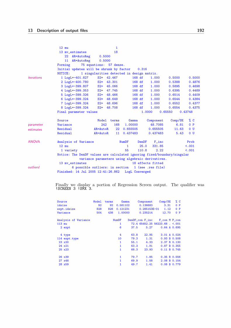
13 Description of output files 192

12 mu 1

13 mv_estimates 18

22 AR=AutoReg 0.5000

11 AR=AutoReg 0.5000

Forming 75 equations: 57 dense.

Initial updates will be shrunk by factor 0.316

NOTICE: 1 singularities detected in design matrix.

1 LogL=-401.827 S2= 42.467 168 df 1.000 0.5000 0.5000iterations2 LogL=-400.780 S2= 43.301 168 df 1.000 0.5388 0.4876

3 LogL=-399.807 S2= 45.066 168 df 1.000 0.5895 0.4698

4 LogL=-399.353 S2= 47.745 168 df 1.000 0.6395 0.4489

5 LogL=-399.326 S2= 48.466 168 df 1.000 0.6514 0.4409

6 LogL=-399.324 S2= 48.649 168 df 1.000 0.6544 0.4384

7 LogL=-399.324 S2= 48.696 168 df 1.000 0.6552 0.4377

8 LogL=-399.324 S2= 48.708 168 df 1.000 0.6554 0.4375

Final parameter values 1.0000 0.65550 0.43748

Source Model terms Gamma Component Comp/SE % C

Variance 242 168 1.00000 48.7085 6.81 0 PparameterResidual AR=AutoR 22 0.655505 0.655505 11.63 0 UestimatesResidual AR=AutoR 11 0.437483 0.437483 5.43 0 U

Analysis of Variance NumDF DenDF F_inc ProbANOVA12 mu 1 25.0 331.85 <.001

1 variety 55 110.8 2.22 <.001

Notice: The DenDF values are calculated ignoring fixed/boundary/singular

variance parameters using algebraic derivatives.

13 mv_estimates 18 effects fitted

6 possible outliers: in section 1 (see .res file)outliers!Finished: 14 Jul 2005 12:41:26.862 LogL Converged

Finally we display a portion of Regression Screen output. The qualifier was!SCREEN 3 !SMX 3.

Source Model terms Gamma Component Comp/SE % C

idsize 92 92 0.581102 0.136683 3.31 0 P

expt.idsize 828 828 0.121231 0.285153E-01 1.12 0 P

Variance 504 438 1.00000 0.235214 12.70 0 P

Analysis of Variance NumDF DenDF_con F_inc F_con M P_con

113 mu 1 72.4 65452.25 56223.68 . <.001

2 expt 6 37.5 5.27 0.64 A 0.695

4 type 4 63.8 22.95 3.01 A 0.024

114 expt.type 10 79.3 1.31 0.93 B 0.508

23 x20 1 55.1 4.33 2.37 B 0.130

24 x21 1 63.3 1.91 0.87 B 0.355

25 x23 1 68.3 23.93 0.11 B 0.745

26 x39 1 79.7 1.85 0.35 B 0.556

27 x48 1 69.9 1.58 2.08 B 0.154

28 x59 1 49.7 1.41 0.08 B 0.779

13 Description of output files 193

29 x60 1 59.6 1.46 0.42 B 0.518

30 x61 1 64.0 1.11 0.04 B 0.838

31 x62 1 61.8 2.18 0.09 B 0.770

32 x64 1 55.6 31.48 4.50 B 0.038

33 x65 1 57.8 4.72 6.12 B 0.016

34 x66 1 58.5 1.13 0.03 B 0.872

35 x70 1 59.3 1.71 1.40 B 0.242

36 x71 1 64.4 0.08 0.01 B 0.929

37 x73 1 59.0 1.79 3.01 B 0.088

38 x75 1 59.9 0.04 0.26 B 0.613

39 x91 1 63.8 1.44 1.44 B 0.234

Notice: The DenDF values are calculated ignoring fixed/boundary/singular

variance parameters using empirical derivatives.

129 mv_estimates 9 effects fitted

9 idsize 92 effects fitted ( 7 are zero)

115 expt.idsize 828 effects fitted ( 672 are zero)

127 at(expt,6).type.idsize.meth 9 effects fitted (+ 2199 singular)

128 at(expt,7).type.idsize.meth 10 effects fitted (+ 2198 singular)

LINE REGRESSION RESIDUAL ADJUSTED FACTORS INCLUDED

NO DF SUMSQUARES DF MEANSQU R-SQUARED R-SQUARED 39 38 37 36 35 34 33 32 31 30 29 28 27 26 25 24 23

1 3 0.1113D+02 452 0.2460 0.09098 0.08495 1 1 1 0 0 0 0 0 0 0 0 0 0 0 0 0 0

***** *****

2 3 0.1180D+02 452 0.2445 0.09648 0.09049 1 0 1 1 0 0 0 0 0 0 0 0 0 0 0 0 0

***** *****

3 3 0.1843D+01 452 0.2666 0.01507 0.00853 0 1 1 1 0 0 0 0 0 0 0 0 0 0 0 0 0

4 3 0.1095D+02 452 0.2464 0.08957 0.08353 1 1 0 1 0 0 0 0 0 0 0 0 0 0 0 0 0

5 3 0.1271D+02 452 0.2425 0.10390 0.09795 1 0 0 1 1 0 0 0 0 0 0 0 0 0 0 0 0

***** *****

6 3 0.9291D+01 452 0.2501 0.07594 0.06981 0 1 0 1 1 0 0 0 0 0 0 0 0 0 0 0 0

7 3 0.9362D+01 452 0.2499 0.07652 0.07039 0 0 1 1 1 0 0 0 0 0 0 0 0 0 0 0 0

8 3 0.1357D+02 452 0.2406 0.11091 0.10501 1 0 1 0 1 0 0 0 0 0 0 0 0 0 0 0 0

***** *****

9 3 0.9404D+01 452 0.2498 0.07687 0.07074 0 1 1 0 1 0 0 0 0 0 0 0 0 0 0 0 0

10 3 0.1266D+02 452 0.2426 0.10350 0.09755 1 1 0 0 1 0 0 0 0 0 0 0 0 0 0 0 0

11 3 0.1261D+02 452 0.2427 0.10313 0.09717 1 0 0 0 1 1 0 0 0 0 0 0 0 0 0 0 0

12 3 0.9672D+01 452 0.2492 0.07906 0.07295 0 1 0 0 1 1 0 0 0 0 0 0 0 0 0 0 0

13 3 0.9579D+01 452 0.2494 0.07830 0.07218 0 0 1 0 1 1 0 0 0 0 0 0 0 0 0 0 0

14 3 0.9540D+01 452 0.2495 0.07797 0.07185 0 0 0 1 1 1 0 0 0 0 0 0 0 0 0 0 0

15 3 0.1089D+02 452 0.2465 0.08907 0.08302 1 0 0 1 0 1 0 0 0 0 0 0 0 0 0 0 0

16 3 0.2917D+01 452 0.2642 0.02384 0.01736 0 1 0 1 0 1 0 0 0 0 0 0 0 0 0 0 0

17 3 0.2248D+01 452 0.2657 0.01838 0.01187 0 0 1 1 0 1 0 0 0 0 0 0 0 0 0 0 0

18 3 0.1111D+02 452 0.2460 0.09088 0.08484 1 0 1 0 0 1 0 0 0 0 0 0 0 0 0 0 0

19 3 0.1746D+01 452 0.2668 0.01427 0.00773 0 1 1 0 0 1 0 0 0 0 0 0 0 0 0 0 0

20 3 0.1030D+02 452 0.2478 0.08423 0.07815 1 1 0 0 0 1 0 0 0 0 0 0 0 0 0 0 0

21 3 0.1279D+02 452 0.2423 0.10454 0.09860 1 0 0 0 0 1 1 0 0 0 0 0 0 0 0 0 0

22 3 0.8086D+01 452 0.2527 0.06609 0.05989 0 1 0 0 0 1 1 0 0 0 0 0 0 0 0 0 0

23 3 0.7437D+01 452 0.2542 0.06079 0.05456 0 0 1 0 0 1 1 0 0 0 0 0 0 0 0 0 0

24 3 0.1071D+02 452 0.2469 0.08755 0.08149 0 0 0 1 0 1 1 0 0 0 0 0 0 0 0 0 0

25 3 0.1370D+02 452 0.2403 0.11200 0.10611 0 0 0 0 1 1 1 0 0 0 0 0 0 0 0 0 0

***** *****

26 3 0.1511D+02 452 0.2372 0.12351 0.11770 1 0 0 0 1 0 1 0 0 0 0 0 0 0 0 0 0

***** *****

27 3 0.1353D+02 452 0.2407 0.11064 0.10473 0 1 0 0 1 0 1 0 0 0 0 0 0 0 0 0 0

...

680 3 0.1057D+02 452 0.2472 0.08641 0.08035 1 1 0 0 0 0 0 0 0 0 0 0 0 0 0 0 1

The .sln file

The .sln file contains estimates of the fixed and random effects with their stan-dard errors in an array with four columns ordered as

13 Description of output files 194

factor name level estimate standard error

Note that the error presented for the estimate of a random effect is the squareroot of the prediction error variance. In a genetic context for example wherea relationship matrix A is involved, the accuracy is

√(1− s2

i

(1+fi)σ2A) where si is

the standard error reported with the BLUP (ui) for the ith individual, fi is theinbreeding coefficient reported when !DIAG qualifier is given on a pedigree fileline, 1+fi is the diagonal element of A and σ2

A is the genetic variance. The .slnfile can easily be read into a GENSTAT spreadsheet or an S-PLUS data frame.Below is a truncated copy of nin89a.sln. Note that

• the order of some terms may differ from the order in which those terms werespecified in the model statement,

• the missing value estimates appear at the end of the file in this example.

variety LANCER 0.000 0.000variety estimates

variety BRULE 2.987 2.842

variety REDLAND 4.707 2.978

variety CODY -0.3131 2.961

variety ARAPAHOE 2.954 2.727...

variety NE87615 1.035 2.934

variety NE87619 5.939 2.850

variety NE87627 -4.376 2.998

mu 1 24.09 2.465intercept

mv_estimates 1 21.91 6.729missing value

mv_estimates 2 23.22 6.721estimates

mv_estimates 3 22.52 6.708

mv_estimates 4 23.49 6.676

mv_estimates 5 22.26 6.698

mv_estimates 6 24.47 6.707

mv_estimates 7 20.14 6.697

mv_estimates 8 25.01 6.691

mv_estimates 9 24.29 6.676

mv_estimates 10 26.30 6.658

mv_estimates 11 24.99 6.590

mv_estimates 12 27.78 6.492...

13 Description of output files 195

The .yht file

The .yht file contains the predicted values of the data in the original order (thisis not changed by supplying row/column order in spatial analyses), the residualsand the diagonal elements of the hat matrix. Figure 13.1 shows the residualsplotted against the fitted values (Yhat) and a line printer version of this figure iswritten to the .res file. Where an observation is missing, the residual, missingvalues predicted value and Hat value are also declared missing. The missing valueestimates with standard errors are reported in the .sln file.

NIN alliance trial 1989 Residuals vs Fitted values Residuals (Y)−24.87:15.91 Fitted values (X) 16.77: 35.94

Figure 13.1 Residual versus Fitted values

This is the first 20 lines of nin89a.yht. Note that the values corresponding tothe missing data (first 15 records) are all -0.1000E-36 which is the internal valueused for missing values.

Record Yhat Residual Hat

1 -0.10000E-36 -0.1000E-36 -0.1000E-36

2 -0.10000E-36 -0.1000E-36 -0.1000E-36

3 -0.10000E-36 -0.1000E-36 -0.1000E-36

4 -0.10000E-36 -0.1000E-36 -0.1000E-36

5 -0.10000E-36 -0.1000E-36 -0.1000E-36

6 -0.10000E-36 -0.1000E-36 -0.1000E-36

7 -0.10000E-36 -0.1000E-36 -0.1000E-36

8 -0.10000E-36 -0.1000E-36 -0.1000E-36

9 -0.10000E-36 -0.1000E-36 -0.1000E-36

10 -0.10000E-36 -0.1000E-36 -0.1000E-36

13 Description of output files 196

11 -0.10000E-36 -0.1000E-36 -0.1000E-36

12 -0.10000E-36 -0.1000E-36 -0.1000E-36

13 -0.10000E-36 -0.1000E-36 -0.1000E-36

14 -0.10000E-36 -0.1000E-36 -0.1000E-36

15 -0.10000E-36 -0.1000E-36 -0.1000E-36

16 24.088 5.162 6.074

17 27.074 4.476 6.222

18 28.795 6.255 6.282

19 23.775 6.325 6.235

20 27.042 6.008 5.962...

240 24.695 1.855 6.114

241 25.452 0.1475 6.158

242 22.465 4.435 6.604

13.4 Other ASReml output files

The .aov file

This file reports details of the ANOVA calculations, particularly as relating tothe conditional F-statistics (not computed in this run). In the following tablerelating to the incremental F-statistic, the columns are

• model term

• columns in design matrix

• numerator degrees of freedom

• simple F-statistic

• F-statistic scaled by λ

• λ as defined in Kenward & Roger.

• denominater degrees of freedom

mu 1 1 331.8483 331.8483 1.0000 25.0082

variety 56 55 2.2259 2.2259 0.9995 110.8419

A more useful example is obtained by adding a linear nitrogen contrast to theoats example (Section 15.2).

13 Description of output files 197

Split plot analysis - oat

blocks *

nitrogen !A

subplots

variety !A

wplots *

yield

oats.asd !skip 2

!CONTRAST linNitr nitrogen .6,

0.4 0.2 0.0

!FCON

yield ∼ mu variety linNitr,

nitrogen variety.linNitr,

v ariety.nitrogen,

!r blocks blocks.wplots

The basic design is six replicates of threewhole plots to which variety was randomised,and four subplots which received 4 rates ofnitrogen. A !CONTRAST qualifier defines themodel term linNitr as the linear covariaterepresenting ntrogen applied. Fitting this be-fore the model term nitrogen means that thislatter term represents lack of fit from a linearresponse.

The !FCON qualifier requests conditional F-statistics. As this is a small example, denom-inator degrees of freedom are reported by de-fault. An extract from the .asr file is followedby the contents of the .aov file.

Degrees of Freedom and Stratum Variances

5.00 3175.06 12.0 4.0 1.0

10.00 601.331 0.0 4.0 1.0

45.00 177.083 0.0 0.0 1.0

Source Model terms Gamma Component Comp/SE % C

blocks 6 6 1.21116 214.477 1.27 0 P

blocks.wplots 18 18 0.598937 106.062 1.56 0 P

Variance 72 60 1.00000 177.083 4.74 0 P

Analysis of Variance NumDF DenDF_con F_inc F_con M P_con

8 mu 1 6.0 245.14 138.14 . <.001

4 variety 2 10.0 1.49 1.49 A 0.272

7 linNitr 1 45.0 110.32 110.32 a <.001

2 nitrogen 2 45.0 1.37 1.37 A 0.265

9 variety.linNitr 2 45.0 0.48 0.48 b 0.625

10 variety.nitrogen 4 45.0 0.22 0.22 B 0.928

The analysis shows that there is a significant linear response to nitrogen level butthe lack of fit term and the interactions with variety are not significant. In thisexample, the conditional F-statistic is the same as the incremental one becausethe contrast must appear before the lack-of-fit and the main effect before theinteraction and otherwise it is a balanced analysis.

The first part of the .aov file, the FMAP table only appears if the job is runin DEBUG mode. There is a line for each model term showing the number

13 Description of output files 198

of non-singular effects in the terms before the current term is absorbed. Forexample, variety.nitrogen initially has 12 degrees of freedom (non-singular ef-fects). mu takes 1, variety then takes 2, linNitr takes 1, nitrogen takes 2,variety.linNitr takes 2 and there are four degrees of freedom left. This infor-mation is used to make sure that the conditional F-statistic does not contradictmarginality principles.

The next table indicates the details of the conditional F-statistic. The conditionalF-statistic is based in the reduction in Sums of Squares from dropping the par-ticular term (indicated by *) from the model also including the terms indicatedby I, C and c.

The next two tables, based on incremental and conditional sums of squares reportthe model term, the number of effects in the term, the (numerator) degrees offreedom, the F-statistic, an adjusted F-statistic multiplied by a scaling constantreported in the next column and finally the computed denominator degrees offreedom. The scaling constant is discussed by Kenward and Roger (1997).

Table showing the reduction in the numerator degrees of freedom

for each term as higher terms are absorbed.

Model Term 6 5 4 3 2 1

1 mu 12 3 4 1 3 1

2 variety 11 3 3 1 2

3 LinNitr 9 3 3 1

4 nitrogen 8 2 2

5 variety.LinNitr 6 2

6 variety.nitrogen 4

Marginality pattern for F-con calculation

-- Model terms --

Model Term DF 1 2 3 4 5 6

1 mu 1 * . C . C .

2 variety 2 I * C C . .

3 LinNitr 1 I I * . . .

4 nitrogen 2 I I I * . .

5 variety.LinNitr 2 I I I I * .

6 variety.nitrogen 4 I I I I I *

F-inc tests the additional variation explained when the term (*)

is added to a model consisting of the I terms.

F-con tests the additional variation explained when the term (*)

is added to a model consisting of the I and C/c terms.

The . terms are ignored for both F-inc and F-con tests.

13 Description of output files 199

Incremental F statistics - calculation of Denominator degrees of freedom

Source Size NumDF F-value Lambda*F Lambda DenDF

mu 1 1 245.1409 245.1409 1.0000 5.0000

variety 3 2 1.4853 1.4853 1.0000 10.0000

LinNitr 1 1 110.3232 110.3232 1.0000 45.0000

nitrogen 4 2 1.3669 1.3669 1.0000 45.0000

variety.LinNitr 3 2 0.4753 0.4753 1.0000 45.0000

variety.nitrogen 12 4 0.2166 0.2166 1.0000 45.0000

Conditional F statistics - calculation of Denominator degrees of freedom

Source Size NumDF F-value Lambda*F Lambda DenDF

mu 1 1 327.5462 327.5462 1.0000 6.0475

variety 3 2 1.4853 1.4853 1.0000 10.0000

LinNitr 1 1 110.3232 110.3232 1.0000 45.0000

nitrogen 4 2 1.3669 1.3669 1.0000 45.0000

variety.LinNitr 3 2 0.4753 0.4753 1.0000 45.0000

variety.nitrogen 12 4 0.2166 0.2166 1.0000 45.0000

The .dpr file

The .dpr file contains the data and residuals from the analysis in double pre-cision binary form. The file is produced when the !RES qualifier (Table 4.3) isinvoked. The file could be renamed with filename extension .dbl and used forinput to another run of ASReml. Alternatively, it could be used by another For-tran program or package. Factors will have level codes if they were coded using!A or !I. All the data from the run plus an extra column of residuals is in thefile. Records omitted from the analysis are omitted from the file.

The .pvc file

The .pvc file contains functions of the variance components produced by runninga .pin file on the results of an ASReml run as described in Chapter 11. The .pinand .pvc files for a half-sib analysis of the Coopworth data are presented inSection 15.10.

The .pvs file

The .pvs file contains the predicted values formed when a predict statement isincluded in the job. Below is an edited version of nin89a.pvs. See Section 3.6for the .pvs file for the simple RCB analysis of the NIN data considered in thatchapter.

nin alliance trial 14 Jul 2005 12:41:18title line

nin89a

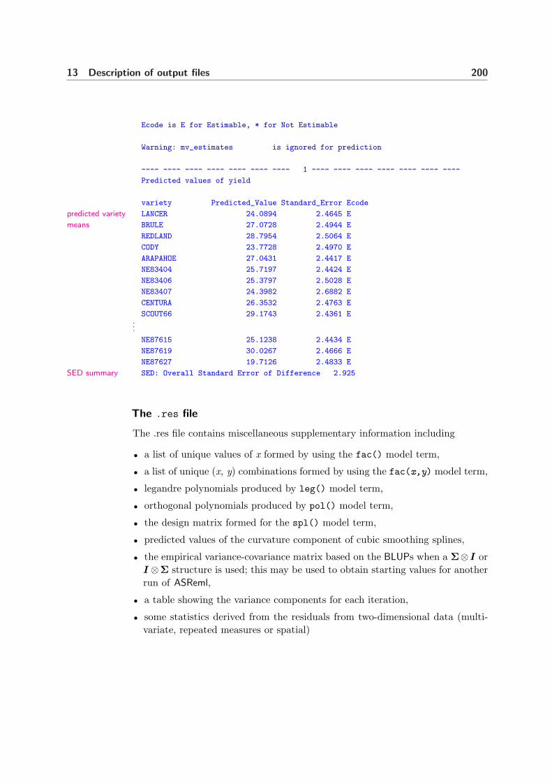
13 Description of output files 200

Ecode is E for Estimable, * for Not Estimable

Warning: mv_estimates is ignored for prediction

---- ---- ---- ---- ---- ---- ---- 1 ---- ---- ---- ---- ---- ---- ----

Predicted values of yield

variety Predicted_Value Standard_Error Ecode

LANCER 24.0894 2.4645 Epredicted variety

BRULE 27.0728 2.4944 Emeans

REDLAND 28.7954 2.5064 E

CODY 23.7728 2.4970 E

ARAPAHOE 27.0431 2.4417 E

NE83404 25.7197 2.4424 E

NE83406 25.3797 2.5028 E

NE83407 24.3982 2.6882 E

CENTURA 26.3532 2.4763 E

SCOUT66 29.1743 2.4361 E...

NE87615 25.1238 2.4434 E

NE87619 30.0267 2.4666 E

NE87627 19.7126 2.4833 E

SED: Overall Standard Error of Difference 2.925SED summary

The .res file

The .res file contains miscellaneous supplementary information including

• a list of unique values of x formed by using the fac() model term,

• a list of unique (x, y) combinations formed by using the fac(x,y) model term,

• legandre polynomials produced by leg() model term,

• orthogonal polynomials produced by pol() model term,

• the design matrix formed for the spl() model term,

• predicted values of the curvature component of cubic smoothing splines,

• the empirical variance-covariance matrix based on the BLUPs when a Σ⊗I orI ⊗Σ structure is used; this may be used to obtain starting values for anotherrun of ASReml,

• a table showing the variance components for each iteration,

• some statistics derived from the residuals from two-dimensional data (multi-variate, repeated measures or spatial)

13 Description of output files 201

– the residuals from a spatial analysis will have the units part added tothem (defined as the combined residual) unless the data records were sorted(within ASReml ) in which case the units and the correlated residuals arein different orders (data file order and field order respectively),

– the residuals are printed in the .yht file but the statistics in the .res fileare calculated from the combined residual,

– the Covariance/Variance/Correlation (C/V/C)matrix calculated directlyfrom the residuals; it contains the covariance below the diagonals, the vari-ances on the diagonal and the correlations above the diagonal:The ’FITTED’ matrix is the same as is reported in the .asr file and ifthe Logl has converged is the one you would report; the ’BLUPS’ matrix isclculated from the BLUPS and is provided so it can be used as starting valueswhen a simple initial model has been used and you are wanting to attemptto fit a full unstructured matrix; the rescaled has the variance from theFITTED and the covariance from the BLUPS and might we more suitableas an initial matrix if the variances have been estimated. The FITTED andRESCALEd matrices should not be reported.

– relevant portions of the estimated variance matrix for each term for whichan R structure or a G structure has been associated,

• a variogram and spatial correlations for spatial analysis; the spatial correlationsare based on distance between data points (see Gilmour et al., 1997),

• the slope of the log(absolute residual) on log(predicted value) for assessing pos-sible mean-variance relationships and the location of large residuals. For ex-ample,

SLOPES FOR LOG(ABS(RES)) ON LOG(PV) for section 1

0.99 2.01 4.34

produced from a trivariate analysis reports the slopes. A slope of b suggeststhat y1−b might have less mean variance relationship. If there is no meanvariance relation, a slope of zero is expected. A slope of 1

2 suggests a SQRTtransformation might resolve the dependence; a slope of 1 means a LOG trans-formation might be appropriate. So, for the 3 traits, log(y1), y−1

2 and y−33 are

indicated. This diagnostic strategy works better when based on grouped dataregressing log(standard deviation) on log(mean).

Also,

STND RES 16 -2.35 6.58 5.64

indicates that for the 16th data record, the residuals are -2.35, 6.58 and 5.64times the respective standard deviations. The standard deviation used in this

13 Description of output files 202

test is calculated directly from the residuals rather than from the analysis.They are intended to flag the records with large residuals rather than to pre-cisely quantify their relative size. They are not studentised residuals and aregenerally not relevant when the user has fitted heterogeneous variances.

This is nin89a.res.

Convergence sequence of variance parameters

Iteration 1 2 3 4 5 6

LogL -401.827 -400.780 -399.807 -399.353 -399.326 -399.324

Change % 59 80 83 21 5 1

Adjusted 0 0 0 0 0 0

StepSz 0.316 0.562 1.000 1.000 1.000 1.000

5 0.500000 0.538787 0.589519 0.639457 0.651397 0.654445 0.5

6 0.500000 0.487564 0.469768 0.448895 0.440861 0.438406 -0.6

Plot of Residuals [-24.8730 15.9145] vs Fitted values [ 16.7724 35.9355] RvE

-----------------------------1------------------------------

| 1 |

| 1 |

| 1 1 1 |

1 3 11 112 1 1 21 1 1 1 |

1 211 24 1311 112 1 |

| 1 1 411 111122 12 |

| 1 1 1 4 1 13 1131111132 2 1 2 |

2 1 1 11 2 21221 11 1 2 1 |

| 1 2 1 21 2 1321 1 1 3 2 2 |

------------1-1-------1-11-1-421122---3---------------------

| 1 1 11 1 2 31111 12 1 |

2 1 1 1 11 |

| 1 12 |

| 1 1 1 |

1 1 1 1 |

| 11 1 |

| 21 1 11 |

| |

1 11 |

| 1 |

| 1 |

| 1 |

| 111 1 |

----------------------------1---1---1----1------------------

SLOPES FOR LOG(ABS(RES)) on LOG(PV) for Section 1

0.15

*

*

* ** ***

* ** *** *

** *** *** *** *

********** *****

******************

* * * * ** ******************

* ** ** ** ** ***** ** ************************ ** *

Min Mean Max -24.873 0.27954 15.915 omitting 18 zeros

13 Description of output files 203

Spatial diagnostic statistics of Residuals 22 11

Residual Plot and Autocorrelations

<LOo- +xXH> [se 0.077]

| ++xxx+X|

|--- - O+ + x +x+x>+X |

|o - -- + +++xxx++X++|

|+ + + +x- +xxx+++|

| o -- ++ +- xx+xHxx|

|-+xxx+xXx +++x xX ++x|

|-++ o- +XxxXXx-xXX +++|

|ooL<Oo --++x x+xXx+x+H|

|<<<<<OO-- xX+ -x ++--|

|<O<<LLLoo - -o-+-+ +|

|L<<<<O-OL-o -++x x+ +|

1 0.28 0.38 0.50 0.65 0.77 1.00 0.77 0.65 0.50 0.38 0.28

2 0.17 0.27 0.39 0.51 0.56 0.64 0.56 0.50 0.40 0.32 0.26

3 0.05 0.11 0.19 0.28 0.35 0.42 0.40 0.35 0.30 0.24 0.19

Residuals [Percentage of sigma = 6.979 ]

0 0 0 0 0 0 0 0 0 0 0 0 0 0 0 74 64 90 91 86 65 141

-72 -29 -52 -20 -61 11 -132 26 0 63 15 99 9 37 84 48 110 228 49 131 -20 9

-87 1 -32 -14 -26 -30 -3 37 -6 4 23 32 44 46 109 97 83 67 68 141 69 40

44 11 0 3 6 0 21 41 -15 51 25 32 120 -33 10 58 117 113 109 63 57 25

18 18 -2 -84 -19 -51 -45 18 30 56 -9 -12 53 -41 7 99 123 47 119 181 101 104

-40 29 87 103 81 61 81 130 94 10 55 53 55 106 15 109 153 23 0 50 66 111

-29 75 43 -24 -90 -37 -23 64 130 84 122 129 126 90 -38 91 133 126 -16 57 30 70

-99 -114 -218 -332 -174 -77 -19 -38 -29 58 63 88 4 124 49 101 129 113 45 92 70 198

-257 -333 -352 -319 -253 -166 -152 -52 -28 0 97 135 67 16 -9 -36 96 24 62 48 -27 -29

-227 -167 -356 -335 -183 -179 -189 -118 -124 14 -52 19 -7 -56 -81 -33 63 -40 57 -15 24 73

-183 -277 -352 -323 -288 -151 -56 -130 -188 -29 -78 7 12 -30 39 57 89 -3 116 27 2 64

| | | |

| | ’ | |

| , ,,, ’| , , , ’ | ,,,,,’, |

|----------------’---’-|---,-,-’,’,-,’-’--’-,,|-,-,--,’,,’’’’-------’|

| |,’’ ’ |, ’ ’’ |

| | ’ | |

| | | |

| | | |

| | , | |

| ’ ’’, | ,’ ’ ,,| ,,, ,’, , ,’ ,|

|’,,,,-,’,’’’--,’---’’’|,,,-,--,’’,,’-,--’----|-’---’---,’’’-,--’-’’-|

| ’ | , ’’ ’ |’ |

| | | |

| | | |

| | | |

| | ,| |

| , ’,’’’, ,’’ ,| , ’ ,’’ ,, | ,’, , |

|--’----’----------,’’-|------,--’’-,-’---’---|-------------,,--’’’--|

|’ ’,’’ ’ |, , ’’ | ’’ ’ ’’|

| | ’ , | ,’ |

| | ’* |,***, |

| | |

| | |

| ,| , ’ |

13 Description of output files 204

|---------,-,,---’-’,’-|-----------,,-’’-,-’,’|

| ’ ’,’ ’ | ’ ’, ’ |

| , ,,,’’ |, ’ ’, |

|’ ** | ,**, |

Residual [section 1, column 8 ( 11), row 4 ( 22)] is -3.32 SD

Residual [section 1, column 9 ( 11), row 2 ( 22)] is -3.33 SD

Residual [section 1, column 9 ( 11), row 3 ( 22)] is -3.52 SD

Residual [section 1, column 10 ( 11), row 3 ( 22)] is -3.56 SD

Residual [section 1, column 10 ( 11), row 4 ( 22)] is -3.35 SD

Residual [section 1, column 11 ( 11), row 3 ( 22)] is -3.52 SD

6 possible outliers in section 1 : test value

23.0311757288330

Figures 13.2 to 13.5 show the graphics derived from the residuals when the!DISPLAY 15 qualifier is specified and which are written to .eps files by run-ning

ASReml -g22 nin89a.as

The graphs are a variogram of the residuals from the spatial analysis for site 1(Figure 13.2), a plot of the residuals in field plan order (Figure 13.3), plots ofthe marginal means of the residuals (Figure 13.4) and a histogram of the resid-uals (Figure 13.5). The selection of which plots are displayed is controlled bythe !DISPLAY qualifier (Table 5.4). By default, the variogram and field plan aredisplayed.

NIN alliance trial 1989 9a 1 Variogram of residuals 14 Jul 2005 12:41:18

0

3.964625

Outer displacement Inner displacement

Figure 13.2 Variogram of residuals

13 Description of output files 205

The sample variogram is a plot of the semi-variances of differences of residuals atparticular distances. The (0,0) position is zero because the difference is identicallyzero. ASReml displays the plot for distances 0, 1, 2, ..., 8, 9-10, 11-14, 15-20, . . . .

The plot of residuals in field plan order (Figure 13.3) contains in its top and rightmargins a diamond showing the minimum, mean and maximum residual for thatrow or column. Note that a gap identifies where the missing values occur.

The plot of marginal means of residuals shows residuals for each row/column aswell as the trend in their means.

NIN alliance trial 1989 9a 1 Field plot of residuals 14 Jul 2005 12:41:18

Range: −24.87 15.91

Figure 13.3 Plot of residuals in field plan order

The .rsv file

The .rsv file contains the variance parameters from the most recent iterationof a model. The primary use of the .rsv file is to supply the values for the!CONTINUE qualifier (see Table 5.4) and the C command line option (see Table12.1). It contains sufficient information to match terms so that it can be usedwhen the variance model has been changed. This is nin89a.rsv.

76 6 1690 120

0.000000 0.000000 0.000000 1.000000 0.6555046 0.4374830

RSTRUCTURE 1 2

VARIANCE 1 1 0 1.00000

STRUCTURE 22 1 1 0.655505

NIN alliance trial 1989 9a 1Residuals V Row and Column position: 14 Jul 2005 12:41:18Range: −24.87 15.91

Figure 13.4 Plot of the marginal means of the residuals

NIN alliance trial 1989 vE_AHistogram of residuals14 Jul 2005 12:41:18

Range: −24.87 15.91Peak Count: 17

0

Figure 13.5 Histogram of residuals

13 Description of output files 207

STRUCTURE 11 1 1 0.437483

The .tab file

The .tab file contains the simple variety means and cell frequencies. Below is anedited version of nin89.tab.

nin alliance trial 10 Sep 2002 04:20:15

Simple tabulation of yield

variety

LANCER 28.56 4

BRULE 26.07 4

REDLAND 30.50 4

CODY 21.21 4

ARAPAHOE 29.44 4

NE83404 27.39 4

NE83406 24.28 4

NE83407 22.69 4

CENTURA 21.65 4

SCOUT66 27.52 4

COLT 27.00 4...

NE87615 25.69 4

NE87619 31.26 4

NE87627 23.23 4

The .vrb file

The .vrb file contains the estimates of the effects together with their approxi-mate prediction variance matrix corresponding to the dense portion. The file isformatted for reading back for post processing. The number of equations in thedense portion can be increased (to a maximum of 800) using the !DENSE option(Table 5.5) but not to include random effects. The matrix is lower triangularrow-wise in the order that the parameters are printed in the .sln file. It can bethought of as a partitioned lower triangular matrix,

σ2 .

βD

σ2CDD

13 Description of output files 208

where βD

is the dense portion of β and CDD

is the dense portion of C−1. Thisis the first 20 rows of nin89a.vrb. Note that the first element is the estimatederror variance, that is, 48.6802, see the variance component estimates in the .asroutput.

0.486802E + 02 0.000000E + 00 0.000000E + 00 0.298660E + 01 0.000000E + 00

0.807551E + 01 0.470711E + 01 0.000000E + 00 0.456648E + 01 0.886687E + 01

−0.313123E + 00 0.000000E + 00 0.410031E + 01 0.476546E + 01 0.876708E + 01

0.295404E + 01 0.000000E + 00 0.343331E + 01 0.389620E + 01 0.416124E + 01

0.743616E + 01 0.163302E + 01 0.000000E + 00 0.377176E + 01 0.428109E + 01

0.472519E + 01 0.402696E + 01 0.837281E + 01 0.129013E + 01 0.000000E + 00

0.330076E + 01 0.347471E + 01 0.357605E + 01 0.316915E + 01 0.412130E + 01

0.768275E + 01 0.310018E + 00 0.000000E + 00 0.376637E + 01 0.419780E + 01

0.395693E + 01 0.383429E + 01 0.458492E + 01 0.378585E + 01 0.985202E + 01

0.226478E + 01 0.000000E + 00 0.379286E + 01 0.442457E + 01 0.439485E + 01

0.402503E + 01 0.440539E + 01 0.362391E + 01 0.502071E + 01 0.901191E + 01

0.508553E + 01 0.000000E + 00 0.393626E + 01 0.430512E + 01 0.423753E + 01

0.428826E + 01 0.417864E + 01 0.363341E + 01 0.444776E + 01 0.527289E + 01

0.855241E + 01 0.243687E + 01 0.000000E + 00 0.351386E + 01 0.369983E + 01

0.384055E + 01 0.330171E + 01 0.362019E + 01 0.352370E + 01 0.359516E + 01

0.392097E + 01 0.406762E + 01 0.801579E + 01 0.475935E + 01 0.000000E + 00

...

The first 5 rows of the lower triangular matrix in this case are

48.68020 0

2.98660 0 8.075514.70711 0 4.56648 8.86687

−0.313123 0 4.10031 4.76546 8.76708...

......

......

. . .

The .vvp file

The .vvp file contains the inverse of the average information matrix on the com-ponents scale. The file is formatted for reading back under the control of the.pin file described in Chapter 11. The matrix is lower triangular row-wise in theorder the parameters are printed in the .asr file. This is nin89a.vvp with theparameter estimates in the order error variance, spatial row correlation, spatialcolumn correlation.

Variance of Variance components 3

51.0852

0.217089 0.318058E-02

0.677748E-01 -0.201181E-02 0.649355E-02

13 Description of output files 209

13.5 ASReml output objects and where to find them

Table 13.2 presents a list of objects produced with each ASReml run and whereto find them in the output files.

Table 13.2: ASReml output objects and where to find them

output object found in comment

analysis of variancetable

.asr file the analysis of variance table contains F-statisticsfor each term in the fixed part of the model. Theseprovide for an incremental or optionally a condi-tional test of significance (see Section 6.12).

data summary .asr file.ass file

includes the number of records read and retainedfor analysis, the minimum, mean, maximum,number of zeros, number of missing values perdata field, factor/variate field distinction.

An extended report of the data is written to the.ass file if the !SUM qualifier is specified. It in-cludes cell counts for factors, histograms of vari-ates and simple correlations among variates

eigen analysis .res file.asl file

When ASReml reports a variance matrix to the.asr file, it also reports an eigen analysis of thematrix (eigen values and eigen vectors) to the.res file.

elapsed time .asr file.asl file

this can be determined by comparing the starttime with the finishing time.

The execution times for parts of the Iteration pro-cess are written to the .asl file if the !DEBUG

!LOGFILE command line qualifiers are invoked.

fixed and random ef-fects

.sln file if !BRIEF -1 is invoked, the effects that were in-cluded in the dense portion of the solution are alsoprinted in the .asr file with their standard error,a t-statistic for testing that effect and a t-statisticfor testing it against the preceding effect in thatfactor.

heritability .pvc file placed in the .pvc file when postprocessing witha .pin file

histogram of residu-als

.res file and graphics file

intermediate results .asl file given if the -DL command line option is used.

13 Description of output files 210

Table of output objects and where to find them ASReml

output object found in comment

mean/variance rela-tionship

.res file for non-spatial analyses ASReml prints the slopeof the regression of log(abs(residual)) againstlog(predicted value). This regression is ex-pected to be near zero if the variance is inde-pendent of the mean. A power of the mean datatransformation might be indicated otherwise. Thesuggested power is approximately (1-b) where b isthe slope. A slope of 1 suggests a log transfor-mation. This is indicative only and should notbe blindly applied. Weighted analysis or identi-fying the cause of the heterogeneity should alsobe considered. This statistic is not reliable in ge-netic animal models or when units is included inthe linear model because then the predicted valueincludes some of the residual.

observed variance/covariance matrixformed from BLUPsand residuals

.res file for an interaction fitted as random effects, whenthe first [outer] dimension is smaller than the in-ner dimension less 10, ASReml prints an observedvariance matrix calculated from the BLUPs. Theobserved correlations are printed in the upper tri-angle. Since this matrix is not well scaled as an es-timate of the underlying variance component ma-trix, a rescaled version is also printed, scaled ac-cording to the fitted variance parameters. Theprimary purpose for this output is to provide rea-sonable starting values for fitting more complexvariance structure. The correlations may also beof interest. After a multivariate analysis, a sim-ilar matrix is also provided, calculated from theresiduals.

phenotypic variance .pvc file placed in the .pvc file when postprocessing witha .pin file

plot of residualsagainst field position

graphics file

possible outliers .res file these are residuals that are more than 3.5 stan-dard deviations in magnitude

predicted (fitted) val-ues at the data points

.yht file these in the are printed in the second column

predicted values .pvs file given if a predict statement is supplied in the .asfile.

REML log-likelihood .asr file the REML log-likelihood is given for each iteration.The REML log-likelihood should have converged

13 Description of output files 211

Table of output objects and where to find them ASReml

output object found in comment

residuals .yht file and in binary form in .dpr file; these are printed incolumn 3. Furthermore, for multivariate analysesthe residuals will be in data order (traits withinrecords). However, in a univariate analysis withmissing values that are not fitted, there will befewer residuals than data records - there will beno residual where the data was missing so this canmake it difficult to line up the values unless youcan manipulate them in another program (spread-sheet).

score .asl file given if the -DL command line option is used.

tables of means .tab file.pvs file

simple averages of cross classified data are pro-duced by the tabulate directive to the .tab file.Adjusted means predicted from the fitted modelare written to the .pvs file by the predict direc-tive.

variance of varianceparameters

.vvp file based on the inverse of the average informationmatrix

variance parameters .asr file.res file

the values at each iteration are printed in the.res file. The final values are arranged in a table,printed with labels and converted if necessary tovariances.

variogram graphics file

14 Error messages

Introduction

Common problems

Things to check in the .asr file

An example

Error messages

Warning messages

212

14 Error messages 213

14.1 Introduction

When ASReml finds an inconsistency it prints an error message to the screen (orthe .asl file) and dumps the current information to the .asr file. Below is thescreen output for a job that has been terminated due to an error. If a job has anerror you should

• try and identify the problem from the error message in the Fault: line and thetext of the Last line read: (this appears twice in the file to make it easier tofind),

• check that all labels have been defined and are in the correct case,

• some errors arise from conflicting information; the error may point to some-thing that appears valid but is inconsistent with something earlier in the file,

• reduce to a simpler model and gradually build up to the desired analysis - thisshould help to identify the exact location of the problem.

If the problem is not resolved from the above list, you may need to email CustomerSupport at support@asreml.co.uk. Please send the .as file, (a sample of) thedata, the .asr file and the .asl file produced by running

asreml -dl basename.as

The -dl command line option invokes debug mode and sends all non-graphicsSee Chapter 12

screen output to the .asl file.

In this chapter we show some of the common typographical problems. Errorsarising from attempts to fit an inappropriate model are often harder to resolve.Following is an example of output when the data file is not correctly named or isnot present (ASReml tries to interpret the filename as a variable name when thefile is not found).

ASReml 1.99a [01 Aug 2005] nin alliance trial

Build: c [26 Jul 2005] 32 bit

27 Jul 2005 15:41:25.267 64.00 Mbyte Windows ninerr1memory info

Licensed to: Arthur Gilmour

...

Folder: C:\data\ex\manexworking direc-

tory Warning: FIELD DEFINITION lines should be INDENTED

There is no file called nine.asd

Invalid label for data field: ’nine.asd’ contains a reserved character

14 Error messages 214

or may get confused with a previous label or reserved word

Fault 12 FORMAT error reading data structures

Last line read was: nine.asd !slip 1

Currently defined structures, COLS and LEVELS

1 variety 1 56 0 0 0 0

2 id 1 1 0 0 0 0

3 pid 1 1 0 0 0 0

4 raw 1 1 0 0 0 0

5 repl 1 4 0 0 0 0

6 nloc 1 1 0 0 0 0

7 yield 1 1 0 0 0 0

8 lat 1 1 0 0 0 0

9 long 1 1 0 0 0 0

10 row 1 22 0 0 0 0

11 column 1 11 0 0 0 0

12 nine.asd 0 0 0 0 0 0filename!

ninerr1 C:\data\ex\manex

12 factors defined [max 500].

0 variance parameters [max1500]. 2 special structures

Last line read was: nine.asd !slip 1last line read

12 12 -1 0 8000

Finished: 27 Jul 2005 15:41:26.379 FORMAT error reading data structuresfault message

14.2 Common problems

Common problems in coding ASReml are as follows:

• a variable name has been misspelt; variable names are case sensitive,

• a model term has been misspelt; model term functions and reserved words (mu,Trait, mv, units) are case sensitive,

• the data file name is misspelt or the wrong path has been given - enclose thepathname in quotes (’) if it includes embedded blanks,

• a qualifier has been misspelt or is in the wrong place,

• there is an inconsistency between the variance header line and the structuredefinition lines presented,

• failure to use commas appropriately in model definition lines,

• there is an error in the R structure definition lines,

14 Error messages 215

• there is an error in the G structure definition lines,

– there is a factor name error,– there is a missing parameter,– there are too many/few initial values,

• there is an error in the predict statement,

• model term mv not included in the model when there are missing values in thedata and the model fitted assumes all data is present.

The most common problem in running ASReml is that a variable label is misspelt.

14.3 Things to check in the .asr file

The information that ASReml dumps in the .asr file when an error is encounteredis intended to give you some idea of the particular error:

• if there is no data summary ASReml has failed before or while reading themodel line,

• if ASReml has completed one iteration the problem is probably associated withstarting values of the variance parameters or the logic of the model rather thanthe syntax per se.

Part of the file nin89.asr presented in Chapter 13 is displayed below to indicatethe lines of the .asr file that should be checked. You should check that

• sufficient workspace has been obtained,

• the records read/lines read/records used are correct,

• mean min max information is correct for each variable,

• the Loglikelihood has converged and the variance parameters are stable,

• ANOVA table has the expected degrees of freedom.

ASReml 1.63o [01 Jun 2005] NIN alliance trial 1989

Build: j [01 Jul 2005] 128

14 Jul 2005 12:41:18.360 32.00 Mbyte Windows nin89aworkspace

Licensed to: Arthur Gilmour

...

Folder: C:\data\asr\UG2\manexworking direc-

tory

14 Error messages 216

variety !A

QUALIFIERS: !SKIP 1 !DISPLAY 15

QUALIFIER: !DOPART 1 is active

Reading nin89aug.asd FREE FORMAT skipping 1 lines

Univariate analysis of yield

Using 242 records of 242 readrecords read

Model term Size #miss #zero MinNon0 Mean MaxNon0data summary

1 variety 56 0 0 1 26.4545 56

2 id 0 0 1.000 26.45 56.00

3 pid 18 0 1101. 2628. 4156.

4 raw 18 0 21.00 510.5 840.0

5 repl 4 0 0 1 2.4132 4

6 nloc 0 0 4.000 4.000 4.000

7 yield Variate 18 0 1.050 25.53 42.00

8 lat 0 0 4.300 25.80 47.30

9 long 0 0 1.200 13.80 26.40

10 row 22 0 0 1 11.5000 22

11 column 11 0 0 1 6.0000 11

12 mu 1

13 mv_estimates 18

22 AR=AutoReg 0.5000

11 AR=AutoReg 0.5000

Forming 75 equations: 57 dense.

Initial updates will be shrunk by factor 0.316

NOTICE: 1 singularities detected in design matrix.

1 LogL=-401.827 S2= 42.467 168 df 1.000 0.5000 0.5000

2 LogL=-400.780 S2= 43.301 168 df 1.000 0.5388 0.4876

3 LogL=-399.807 S2= 45.066 168 df 1.000 0.5895 0.4698

4 LogL=-399.353 S2= 47.745 168 df 1.000 0.6395 0.4489

5 LogL=-399.326 S2= 48.466 168 df 1.000 0.6514 0.4409

6 LogL=-399.324 S2= 48.649 168 df 1.000 0.6544 0.4384

7 LogL=-399.324 S2= 48.696 168 df 1.000 0.6552 0.4377

8 LogL=-399.324 S2= 48.708 168 df 1.000 0.6554 0.4375check

convergence

Final parameter values 1.0000 0.65550 0.43748

Source Model terms Gamma Component Comp/SE % Cparameter

estimates Variance 242 168 1.00000 48.7085 6.81 0 P

Residual AR=AutoR 22 0.655505 0.655505 11.63 0 U

14 Error messages 217

Residual AR=AutoR 11 0.437483 0.437483 5.43 0 U

Analysis of Variance NumDF DenDF F_inc ProbANOVA

12 mu 1 25.0 331.85 <.001

1 variety 55 110.8 2.22 <.001

Notice: The DenDF values are calculated ignoring fixed/boundary/singular

variance parameters using algebraic derivatives.

13 mv_estimates 18 effects fitted

6 possible outliers: in section 1 (see .res file)outliers?

Finished: 14 Jul 2005 12:41:26.862 LogL Converged

14.4 An example

nin alliance trial

variety 56 # 3.

id

pid

raw

repl 4

nloc

yield

lat

long

row 22

column 11

nine.asd !slip 1 !dopart $1

# 1. & 2.

!part 1

yield∼mu variety # 4.

!r Repl # 5.

0 0 1

Repl 1 # 6.

2 0 IDV 0.1 # 7.

!part 2

yield∼mu variety # 9.

1 2

11 row AR1 .1 #10.

22 col AR1 .1

!part

predict voriety # 8.

This is the command file for a simple RCBSee 2a in Sec-

tion 7.3 analysis of the NIN variety trial data in thefirst part. However, this file contains eightcommon mistakes in coding ASReml. We alsoshow two common mistakes associated withspatial analyses in the second part. The errorsare highlighted and the numbers indicate theorder in which they are detected. Each error isdiscussed with reference to the output writtento the .asr file. A summary of the errors isas follows:

1. data file not found,

2. unrecognised qualifier,

3. incorrectly defined alphanumeric factor,

4. comma missing from first line of model,

5. misspelt variable label in linear model,

6. misspelt variable label in G structureheader line,

7. wrong levels declared in G structure modelline,

14 Error messages 218

8. misspelt variable label in predict statement.

9. mv omitted from spatial model

10. wrong levels declared in R structure modellines

1. Data file not found

nin alliance trial...

nine.asd !slip 1

yield ∼ mu variety...

Running this job produces the .asr file in Sec-tion 14.1. The first problem is that ASReml

cannot find the data file nine.asd as indi-cated in the error message above the Faultline. ASReml reports the last line read beforethe job was terminated, an error messageFORMAT error reading data structuresand other information obtained to that point. In this case the program only madeit to the data file definition line in the command file. Since nine.asd commencesin column 1, ASReml checks for a file of this name (in the working directory sinceno path is supplied). Since ASReml did not find the data file it tried to interpretthe line as a variable definition but . is not permitted in a variable label. Theproblem is either that the filename is misspelt or a pathname is required. In thiscase the data file was given as nine.asd rather than nin.asd.

2. An unrecognised qualifier and 3. An incorrectly defined factor

After supplying the correct pathname and re-running the job, ASReml producesthe warning message

WARNING: Unrecognised qualifier at character 9 !slip 1

followed by the fault message

ERROR Reading the data.The warning does not cause the job to terminate immediately but arises because!slip is not a recognised data file line qualifier; the correct qualifier is !skip.The job terminates when reading the header line of the nin.asd file which isalphabetic when it is expecting numeric values. The following output displaysthe error message produced.

ASReml 1.99a [01 Aug 2005] nin alliance trial

Build: c [26 Jul 2005] 32 bit

27 Jul 2005 15:41:38.987 64.00 Mbyte Windows ninerr2

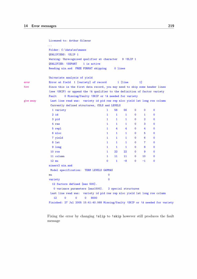
14 Error messages 219

Licensed to: Arthur Gilmour

...

Folder: C:\data\ex\manex

QUALIFIERS: !SLIP 1

Warning: Unrecognised qualifier at character 9 !SLIP 1

QUALIFIER: !DOPART 1 is active

Reading nin.asd FREE FORMAT skipping 0 lines

Univariate analysis of yield

Error at field 1 [variety] of record 1 [line 1]error

Since this is the first data record, you may need to skip some header lineshint

(see !SKIP) or append the !A qualifier to the definition of factor variety

Fault 0 Missing/faulty !SKIP or !A needed for variety

Last line read was: variety id pid raw rep nloc yield lat long row columngive away

Currently defined structures, COLS and LEVELS

1 variety 1 56 56 0 0 0

2 id 1 1 1 0 1 0

3 pid 1 1 1 0 2 0

4 raw 1 1 1 0 3 0

5 repl 1 4 4 0 4 0

6 nloc 1 1 1 0 5 0

7 yield 1 1 1 0 6 0

8 lat 1 1 1 0 7 0

9 long 1 1 1 0 8 0

10 row 1 22 22 0 9 0

11 column 1 11 11 0 10 0

12 mu 0 1 -8 0 -1 0

ninerr2 nin.asd

Model specification: TERM LEVELS GAMMAS

mu 0

variety 0

12 factors defined [max 500].

0 variance parameters [max1500]. 2 special structures

Last line read was: variety id pid raw rep nloc yield lat long row column

12 0 0 0 8000

Finished: 27 Jul 2005 15:41:40.068 Missing/faulty !SKIP or !A needed for variety

Fixing the error by changing !slip to !skip however still produces the faultmessage

14 Error messages 220

Missing/faulty !SKIP or !A needed for variety.

The portion of output given below shows that ASReml has baulked at the nameLANCER in the first field on the first data line. This alphabetic data field is notdeclared as alphabetic. The correct data field definition for variety is

variety !A

to indicate that variety is a character field.

Folder: C:\asr\ex\manex

QUALIFIERS: !SKIP 1

Reading nin89.asd FREE FORMAT skipping 1 lines

Univariate analysis of yield

Field 1 [LANCER] of record 1 [line 1] is not valid.

Since this is the first data record, you may need to skip some header lineshint

(see !SKIP) or append the !A qualifier to the definition of factor variety

Fault 0 Missing/faulty !SKIP or !A needed for variety

Last line read was: LANCER 1 NA NA 1 4 NA 4.3 1.2 1 1

:

ninerr3 variety id pid raw rep nloc yield lat

Model specification: TERM LEVELS GAMMAS

mu 0 0.000

variety 0 0.000

12 factors defined [max 500].

0 variance parameters [max 900]. 2 special structures

Last line read was: LANCER 1 NA NA 1 4 NA 4.3 1.2 1 1

12 0 0 0 8000

Finished: 28 Jul 2005 09:51:12.817 Missing/faulty !SKIP or !A needed for variety

4. A missing comma and 5. A misspelt factor name in linear model

nin alliance trial

variety !A...

repl 4...

nin89.asd !skip 1

yield ∼ mu variety

!r Repl...

The model has been written over two lines butASReml does not realise this because the firstline does not end with a comma. The missingcomma causes the fault

R header SECTIONS DIMNS GSTRUCT

as ASReml tries to interpret the second line ofthe model (see Last line read) as the vari-ance header line. The .asr file is displayed

14 Error messages 221

below. Note that the data has now been suc-cessfully read as indicated by the data summary. You should always check thedata summary to ensure that the correct number of records have been detectedand the data values match the names appropriately.

ASReml 1.99a [01 Aug 2005] nin alliance trial

Build: d [27 Jul 2005] 32 bit

28 Jul 2005 09:53:15.553 64.00 Mbyte Windows ninerr4

Licensed to: Arthur Gilmour

Folder: C:\data\ex\manex

variety !A

QUALIFIERS: !SKIP 1

QUALIFIER: !DOPART 1 is active

Reading nin.asd FREE FORMAT skipping 1 lines

Univariate analysis of yield

Using 224 records of 242 read

Model term Size #miss #zero MinNon0 Mean MaxNon0

1 variety 56 0 0 1 28.5000 56

2 id 0 0 1.000 28.50 56.00

3 pid 0 0 1101. 2628. 4156.

4 raw 0 0 21.00 510.5 840.0

5 repl 4 0 0 1 2.5000 4

6 nloc 0 0 4.000 4.000 4.000

7 yield Variate 0 0 1.050 25.53 42.00

8 lat 0 0 4.300 27.22 47.30

9 long 0 0 1.200 14.08 26.40

10 row 22 0 0 1 11.7321 22

11 column 11 0 0 1 6.3304 11

12 mu 1

Fault 0 R header SECTIONS DIMNS GSTRUCT

Last line read was: !r Repl 0 0 0 0

ninerr4 variety id pid raw rep nloc yield lat

Model specification: TERM LEVELS GAMMAS

variety 56

mu 1

12 factors defined [max 500].

0 variance parameters [max1500]. 2 special structures

Final parameter values

14 Error messages 222

Last line read was: !r Repl 0 0 0 0

12 0 242 224 8000

Finished: 28 Jul 2005 09:53:16.775 R header SECTIONS DIMNS GSTRUCT

Inserting a comma on the end of the first line of the model to give

yield ∼ mu variety,!r Repl

solves that problem but produces the error message

Error reading model factor list

because Repl should have been spelt repl. Portion of the output is displayed.Since the model line is parsed before the data is read, this run failed beforereading the data.

ASReml 1.99a [01 Aug 2005] nin alliance trial

Build: d [27 Jul 2005] 32 bit

28 Jul 2005 10:06:48.042 64.00 Mbyte Windows ninerr5

Licensed to: Arthur Gilmour

Folder: C:\data\ex\manex

variety !A

QUALIFIERS: !SKIP 1

QUALIFIER: !DOPART 1 is active

Reading nin.asd FREE FORMAT skipping 1 lines

Fault 0 Error reading model factor list

Last line read was: Repl

Currently defined structures, COLS and LEVELS

1 variety 1 2 2 0 0 0

2 id 1 1 1 0 1 0

3 pid 1 1 1 0 2 0

4 raw 1 1 1 0 3 0

5 repl 1 4 4 0 4 0

6 nloc 1 1 1 0 5 0

:

Finished: 28 Jul 2005 10:06:49.173 Error reading model factor list

14 Error messages 223

6. Misspelt factor name and 7. Wrong levels declaration in the G struc-ture definition lines

nin alliance trial...

nin89.asd !skip 1

yield ∼ mu variety

!r Repl

0 0 1

Repl 1

2 0 IDV 0.1

The next fault ASReml detects is

G structure header: Factor, order

indicating that there is something wrong inthe G structure definition lines. In this casethe replicate term in the first G structure def-inition line has been spelt incorrectly. To cor-rect this error replace Repl with repl.

ASReml 1.99a [01 Aug 2005] nin alliance trial

Build: c [26 Jul 2005] 32 bit

27 Jul 2005 15:41:52.606 64.00 Mbyte Windows ninerr6

Licensed to: Arthur Gilmour

Folder: C:\data\ex\manex

variety !A

QUALIFIERS: !SKIP 1

QUALIFIER: !DOPART 1 is active

Reading nin.asd FREE FORMAT skipping 1 lines

Univariate analysis of yield

Using 224 records of 242 read

Model term Size #miss #zero MinNon0 Mean MaxNon0

1 variety 56 0 0 1 28.5000 56

2 id 0 0 1.000 28.50 56.00

3 pid 0 0 1101. 2628. 4156.

4 raw 0 0 21.00 510.5 840.0

5 repl 4 0 0 1 2.5000 4

6 nloc 0 0 4.000 4.000 4.000

7 yield Variate 0 0 1.050 25.53 42.00

8 lat 0 0 4.300 27.22 47.30

9 long 0 0 1.200 14.08 26.40

10 row 22 0 0 1 11.7321 22

11 column 11 0 0 1 6.3304 11

12 mu 1

Fault 1 G structure header: Factor, order

Last line read was: Repl 1 0 0 0 0

ninerr6 variety id pid raw rep nloc yield lat

14 Error messages 224

Model specification: TERM LEVELS GAMMAS

variety 56

mu 1

repl 4 0.100

SECTIONS 224 4 1

TYPE 0 0 0

STRUCT 224 0 0 0 0 0 0

12 factors defined [max 500].

4 variance parameters [max1500]. 2 special structures

Final parameter values 0.10000 1.0000

Last line read was: Repl 1 0 0 0 0

12 1 242 224 8000

Finished: 27 Jul 2005 15:41:53.668 G structure header: Factor, order

Fixing the header line, we then get the error message

Structure / Factor mismatch

This arose because repl has 4 levels but we have only declared 2 in the G struc-ture model line. The G structure should read

repl 14 0 IDV 0.1

The last lines of the output with this error are displayed below.

11 column 11 0 0 1 6.3304 11

12 mu 1

2 identity 0.1000

Structure for repl has 2 levels defined

Fault 1 Structure / Factor mismatch

Last line read was: 2 0 IDV 0.1 0 0 0 0 0

ninerr7 variety id pid raw rep nloc yield lat

Model specification: TERM LEVELS GAMMAS

variety 56

mu 1

repl 4 0.100

SECTIONS 224 4 1

TYPE 0 0 1002

STRUCT 224 0 0 0 0 0 0

14 Error messages 225

2 1 0 5 0 1 0

12 factors defined [max 500].

5 variance parameters [max1500]. 2 special structures

Final parameter values 0.10000 1.0000 0.10000

Last line read was: 2 0 IDV 0.1 0 0 0 0 0

12 1 242 224 8000

Finished: 27 Jul 2005 15:41:57.153 Structure / Factor mismatch

8. A misspelt factor name in the predict statement

The final error in the job is that a factor name is misspelt in the predict statement.This is a non-fatal error. The faulty statement is simply ignored by ASReml andno .pvs file is produced. To rectify this statement correct voriety to variety.see Chapter 13

9. Forgetting mv in a spatial analysis

The first error message from running part 2 of the job is

R structures imply 0 + 242 records: only 224 exist

Checking the seventh line of the output below, we see that there were 242 recordsread but only 224 were retained for analysis. There are three reasons records aredropped.1. the !FILTER qualifier has been specified,2. the !D transformation qualifier has been specified and3. there are missing values in the response variable and the user has not specifiedthat they be estimated.The last applies here so we must change the model line to read yield ∼ muvariety mv.

Folder: C:\data\ex\manex

variety !A

QUALIFIERS: !SKIP 1

QUALIFIER: !DOPART 2 is active

Reading nin.asd FREE FORMAT skipping 1 lines

Univariate analysis of yield

Using 224 records of 242 read

Model term Size #miss #zero MinNon0 Mean MaxNon0

1 variety 56 0 0 1 28.5000 56

14 Error messages 226

:

11 column 11 0 0 1 6.3304 11

12 mu 1

11 AR=AutoReg 0.1000

22 AR=AutoReg 0.1000

Maybe you need to include ’mv’ in the model

Fault 1 R structures imply 0 + 242 records: only 224 e

Last line read was: 22 column AR1 0.1 0 0 0 0 0

ninerr9 variety id pid raw rep nloc yield lat

Model specification: TERM LEVELS GAMMAS

variety 56

mu 1

SECTIONS 242 3 1

STRUCT 11 1 1 4 1 1 10

22 1 1 5 1 1 11

12 factors defined [max 500].

5 variance parameters [max1500]. 2 special structures

Final parameter values 0.0000 -.10000E-360.10000

0.10000

Last line read was: 22 column AR1 0.1 0 0 0 0 0

12 1 242 224 8000

Finished: 27 Jul 2005 15:42:10.192 R structures imply 0+242 records: only 224 exist

10. Field layout error in a spatial analysis

The final common error we highlight is the misspecification of the field layout. Inthis case we have ’accidently’ switched the levels in rows and columns. However,ASReml can detect this error because we have also asked it to sort the data intofield order. Had sorting not been requested, ASReml would not have been ableto detect that the lines of the data file were not sorted into the appropriate fieldorder and spatial analysis would be wrong.

:

Folder: C:\data\ex\manex

variety !A

QUALIFIERS: !SKIP 1

QUALIFIER: !DOPART 2 is active

Reading nin.asd FREE FORMAT skipping 1 lines

Univariate analysis of yield

14 Error messages 227

Using 242 records of 242 read

Model term Size #miss #zero MinNon0 Mean MaxNon0

1 variety 56 0 0 1 26.4545 56

:

10 row 22 0 0 1 11.5000 22

11 column 11 0 0 1 6.0000 11

12 mu 1

13 mv_estimates 18

11 AR=AutoReg 0.1000

22 AR=AutoReg 0.1000

Warning: Spatial mapping information for side 1 of order 11

ranges from 1.0 to 22.0

Warning: Spatial mapping information for side 2 of order 22

ranges from 1.0 to 11.0

Fault 2 Sorting data into field order

Last line read was: 22 column AR1 0.1 0 0 0 0 0

ninerr10 variety id pid raw rep nloc yield lat

Model specification: TERM LEVELS GAMMAS

variety 56

mu 1

mv_estimates 18

SECTIONS 242 4 1

STRUCT 11 1 1 5 1 1 10

22 1 1 6 1 1 11

13 factors defined [max 500].

6 variance parameters [max1500]. 2 special structures

Final parameter values 0.0000 -.10000E-360.10000

0.10000

Last line read was: 22 column AR1 0.1 0 0 0 0 0

13 2 242 242 8000

Finished: 27 Jul 2005 15:42:31.733 Sorting data into field order

14 Error messages 228

14.5 Information, Warning and Error messages

ASReml prints information, warning and error messages in the .asr file. Themajor information messages are in Table 14.2. A list of warning messages togetherwith the likely meaning(s) is presented in Table 14.1. Error messages with theirprobable cause(s) is presented in Table 14.3.

Table 14.1: Some information messages and comments

information message comment

Logl converged the REML log-likelihood changes between iter-ations were less than 0.002 * iteration numberand variance parameter values appear stable.

BLUP run done A full iteration has not been completed. Seediscussion of !BLUP.

JOB ABORTED by USER See discussion of ABORTASR.NOW.

Logl converged, parameters not

converged

the change in REML log-likelihood was smalland convergence was assumed but the param-eters are, in fact, still changing.

Logl not converged the maximum number of iterations wasreached before the REML log-likelihood con-verged. Examine the sequence of estimates inthe .res file. You may need more iterationsin which case restart with the !CONTINUE com-mand line option (see Section 12.3 on job con-trol). Otherwise restart with more appropri-ate initial variances. It may be necessary tosimplify the model and estimate the dominantcomponents before estimating other terms.

Warning: Only one iteration

performed

Parameter values are not at the REML solu-tion.

Parameters unchanged after one

iteration.

Parameters appear to be at the REML solu-tion in that the parameter values are stable.

14 Error messages 229

Table 14.2: List of warning messages and likely meaning(s)

warning message likely meaning

Warning: e missing values

generated by !^ transformation

data values should be positive.

Warning: i singularities in AI

matrix

usually means variance model is overparame-terized.

Warning: m variance structures

were modified

the structures are probably at the boundaryof the parameter space.

Warning: n missing values were

detected in the design

either use !MVINCLUDE or delete the records.

Warning: n negative weights it is better to avoid negative weights unless youcan check ASReml is doing the correct thingwith them.

Warning: r records were read

from multiple lines

check you have the intended number of fieldsper line.

WARNING term has more levels [ ##

] than expected [ ## ]:

You have probably mis-specified the numberof levels in the factor or omitted the !I qual-ifier (see Section 5.4 on data field definitionsyntax). ASReml corrects the number of lev-els.

Warning: term in the predict

!IGNORE list

the term did not appear in the model.

Warning: term in the predict

!USE list

the term did not appear in the model.

Warning: term is ignored for

prediction

terms like units and mv cannot be included inprediction.

Warning: Check if you need the

!RECODE qualifier

!RECODE may be needed if the binary file wasnot prepared with ASReml.

Warning: Code B - fixed at a

boundary (!GP)

suggest drop the term and refit the model.

Warning: Eigen analysis check of

US matrix skipped

matrix is probably OK.

WARNING: Extra lines on the end

of the input file ...:

this indicates that there are some lines on theend of the .as file that were not used. Thefirst ”extra” line is displayed. This is only aproblem if you intended ASReml to read theselines.

Warning: Fewer levels found in

termASReml increases to the correct value.

Warning: FIELD DEFINITION lines

should be INDENTED

indent them to avert this message.

14 Error messages 230

List of warning messages and likely meaning(s)

warning message likely meaning

Warning: Fixed levels for factor user nominated more levels than are permit-ted.

Warning: Initial gamma value is

zero

constraint parameter is probably wrongly as-signed.

Warning: Invalid argument. fix the argument.

Warning: It is usual to include

Trait

in multivariate analysis model.

Warning: LogL Converged;

Parameters Not Converged

you may need more iterations.

Warning: LogL not converged restart to do more iterations (see !CONTINUE).

Warning: Missing cells in table missing cells are normally not reported.

Warning: More levels found in

termconsider setting levels correctly.

Warning: PREDICT LINE IGNORED -

TOO MANY

limit is 100.

Warning: PREDICT statement is

being ignored

because it contains errors.

Warning: Second occurrence of

term dropped

if you really want to fit this term twice, createa copy with another name.

Warning: Spatial mapping

information for side

gives details so you can check ASReml is doingwhat you intend.

Warning: Standard errors that is, these standard errors are approximate.

Warning: SYNTAX CHANGE: text may

be invalid

use the correct syntax.

Warning: The !A qualifier

ignored when reading BINARY data

the !A fields will be treated as factors but arenot encoded.

Warning: The !SPLINE qualifier

has been redefined.

use correct syntax.

Warning: The !X !Y !G qualifiers

are ignored. There is no data to

plot

revise the qualifier arguments.

Warning: The estimation was

ABORTED

do not accept the estimates printed.

Warning: The labels for

predictions are erroneous

the labels for predicted terms are probably outof kilter. Try a simpler predict statement. Ifthe problem persists, send for help.

14 Error messages 231

List of warning messages and likely meaning(s)

warning message likely meaning

Warning: This US structure is

not positive definite

check the initial values.

Warning: Unrecognised qualifier

at character

the qualifier either is misspelt or is in thewrong place.

Warning: US matrix was not

positive definite: MODIFIED

the initial values were modified.

Warning: User specified spline

points

the points have been rescaled to suit the datavalues.

Warning: Variance parameters

were modified by BENDing

ASReml may not have converged to the bestestimate.

WARNING Likelihood decreased.

Check gammas and singularities.:

a common reason is that some constraints haverestricted the gammas. Add the !GU qualifierto any factor definition whose gamma valueis approaching zero (or the correlation is ap-proaching (-)1. Alternatively, more singular-ities may have been detected. You shouldidentify where the singularities are expectedand modify the data so that they are omittedor consistently detected. One possibility is tocentre and scale covariates involved in interac-tions so that their standard deviation is closeto 1.

Table 14.3: Alphabetical list of error messages and probablecause(s)/remedies

error message probable cause/remedy

!PRINT: Cannot open output file Check filename.

AINV/GIV matrix undefined or

wrong size

Check the size of the factor associated withthe AINV/GIV structure.

ASReml command file is EMPTY: The job file should be in ASCII format.

ASReml failed in ... Try running the job with increased workspace,or using a simpler model. Otherwise send thejob to VSN (mailto:support@asreml.co.uk)for investigation.

14 Error messages 232

Alphabetical list of error messages and probable cause(s)/remedies

error message probable cause/remedy

Continue from .rsv file Try running without the !CONTINUE qualifier.

Convergence failed the program did not proceed to convergencebecause the REML log-likelihood was fluctuat-ing wildly. One possible reason is that somesingular terms in the model are not being de-tected consistently. Otherwise, the updated Gstructures are not positive definite. There aresome things to try:

– define US structures as positive definite byusing !GP,

– supply better starting values,

– fix parameters that you are confident ofwhile getting better estimates for others(that is, fix variances when estimating co-variances),

– fit a simpler model,

– reorganise the model to reduce covarianceterms (for example, use CORUH instead ofUS.)

Correlation structure is not

positive definite

It is best to start with a positive definite corre-lation structure. Maybe use a structured cor-relation matrix.

Define structure for ... A variance structure should be specified forthis term.

Error in !CONTRAST label factor

values

The error could be in the variable(factor)name or in the number of values or the listof values.

Error in !SUBSET label factor

values

The error could be in the variable(factor)name or in the number of values or the listof values.

Error in R structure: model

checks

the error model is not correctly specified.

Error opening file the file did not exist or was of the wrong filetype (binary = unformatted, sequential).

Error reading something There are several messages of this form wheresomething is what ASReml is attempting toread. Either there is an error telling ASRemlto read something when it does not need to,or there is an error in the way something isspecified.

14 Error messages 233

Alphabetical list of error messages and probable cause(s)/remedies

error message probable cause/remedy

Error reading the data: the data file could not be interpreted: al-phanumeric fields need the !A qualifier.

Error reading the DATA FILENAME

line

data file name may be wrong

Error reading the model factor

list

the model specification line is in error: a vari-able is probably misnamed.

Error setting constraints (!VCC)

on variance components

The !VCC constraints are specified last of alland require knowing the position of each pa-rameter in the parameter vector.

Error setting dependent variable the specified dependent variable name is notrecognised.

Error setting MBF design matrix:

!MBF mbf(x,k) filename

It is likely that the covariate values to notmatch the values supplied in the file. The val-ues in the file should be in sorted order.

Error structures are wrong size: the declared size of the error structures doesnot match the actual number of data records.

Error when reading knot point

values

There is some problem on the !SPLINE line. Itcould be a wrong variable name or the wrongnumber of knot points. Knot points should bein increasing order.

Failed forming R/G scores...? Try increasing workspace.

Failed ordering Level labels The problem may be due to the use of the!SORT qualifier.

Failed to parse R/G structure

line

Failed to read R/G structure line

May be an unrecognised factor/model-termname or variance structure name or wrongcount of initial values, possible on an earlierline. May be insufficient lines in the job.

Failed to process MYOWNGDG files Check your MYOWNGDG program and the.gdg file.

Failed when sorting pedigree ...

Failed when processing pedigree

file ...

Maybe increase !WORKSPACE.

Failed while ordering equations. Try increasing the workspace or simplifyingthe model.

14 Error messages 234

Alphabetical list of error messages and probable cause(s)/remedies

error message probable cause/remedy

FORMAT error reading factor

Definitions:

Likely causes are

– bad syntax or invalid characters in the vari-able labels; variable labels must not includeany of these symbols; !|-+(:#$ and .,

– the data file name is misspelt,

– there are too many variables declared orthere is no valid value supplied with anarithmetic transformation option.

G-structure header: Factor

order:

there is a problem reading G structure headerline. The line must contain the name of a termin the linear model spelt exactly as it appearsin the model

G structure: ORDER 0 MODEL

GAMMAS:

a G structure line cannot be interpreted.

G structure size does not match The size of the structure defined does not agreewith the model term that it is associated with.

Gamma Constraint READ error Check the syntax.

Getting Pedigree: an error occurred processing the pedigree. Thepedigree file must be ascii, free format withANIMAL, SIRE and DAM as the first three fields.

GLM Bounds failure ASReml failed to calculate the GLM workingvariables or weights. Check the data.

Increase declared levels for

factor ...

Either the field has alphanumeric values buthas not been declared using the !A qualifier,or there is not enough space to hold the levelsof the factor. To ’increase the levels’, insertthe expected number of levels after the !A or!I qualifier in the field definition.

Increase workspace ... Use !WORKSPACE s to increase theworkspace available to ASReml . If the dataset is not extremely big, check the datasummary.

Insufficient data read from file Maybe the response variable is all missing.

Insufficient points for : there must be at least 3 distinct data valuesfor a spline term

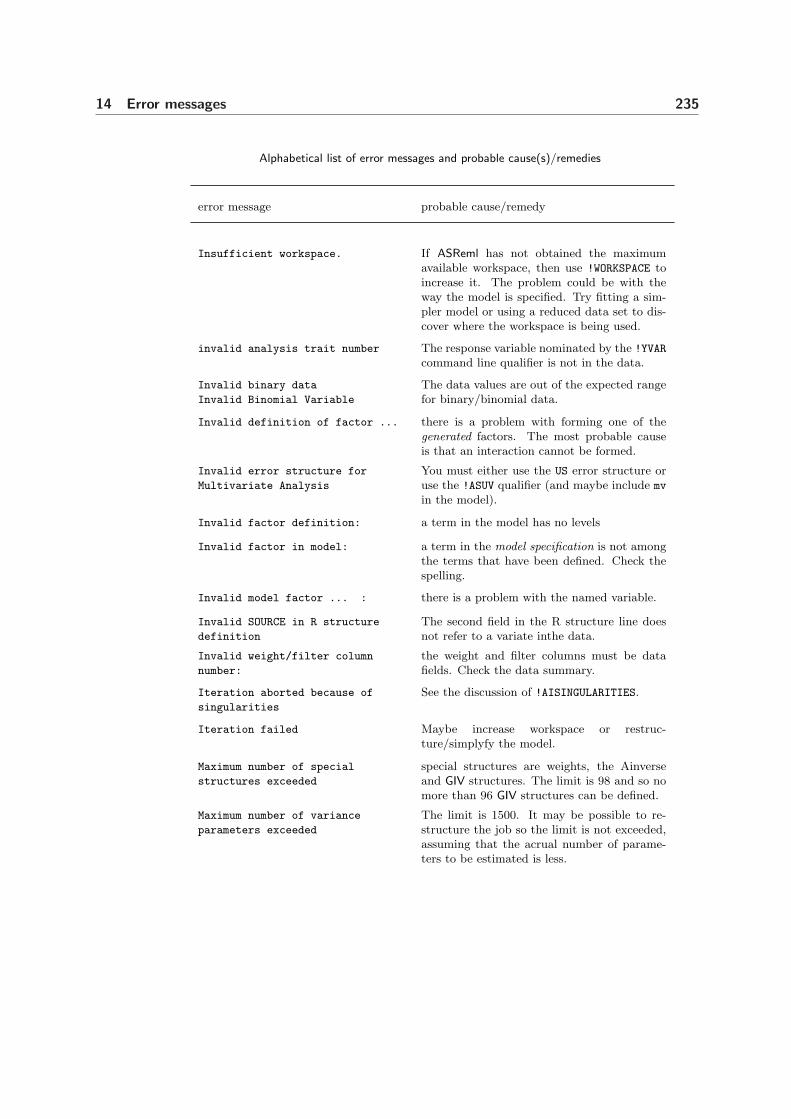
14 Error messages 235

Alphabetical list of error messages and probable cause(s)/remedies

error message probable cause/remedy

Insufficient workspace. If ASReml has not obtained the maximumavailable workspace, then use !WORKSPACE toincrease it. The problem could be with theway the model is specified. Try fitting a sim-pler model or using a reduced data set to dis-cover where the workspace is being used.

invalid analysis trait number The response variable nominated by the !YVARcommand line qualifier is not in the data.

Invalid binary data

Invalid Binomial Variable

The data values are out of the expected rangefor binary/binomial data.

Invalid definition of factor ... there is a problem with forming one of thegenerated factors. The most probable causeis that an interaction cannot be formed.

Invalid error structure for

Multivariate Analysis

You must either use the US error structure oruse the !ASUV qualifier (and maybe include mv

in the model).

Invalid factor definition: a term in the model has no levels

Invalid factor in model: a term in the model specification is not amongthe terms that have been defined. Check thespelling.

Invalid model factor ... : there is a problem with the named variable.

Invalid SOURCE in R structure

definition

The second field in the R structure line doesnot refer to a variate inthe data.

Invalid weight/filter column

number:

the weight and filter columns must be datafields. Check the data summary.

Iteration aborted because of

singularities

See the discussion of !AISINGULARITIES.

Iteration failed Maybe increase workspace or restruc-ture/simplyfy the model.

Maximum number of special

structures exceeded

special structures are weights, the Ainverseand GIV structures. The limit is 98 and so nomore than 96 GIV structures can be defined.

Maximum number of variance

parameters exceeded

The limit is 1500. It may be possible to re-structure the job so the limit is not exceeded,assuming that the acrual number of parame-ters to be estimated is less.

14 Error messages 236

Alphabetical list of error messages and probable cause(s)/remedies

error message probable cause/remedy

Missing/faulty !SKIP or !A needed

for ...

ASReml failed to read the first data record.Maybe it is a heading line which should beskipped by using the !SKIP qualifier, or maybethe field is an alphanumeric field but has notbeen declared so with the !A qualifier.

Missing values in design

variables/factors

You need to identify which design terms con-tain missing values and decide whether deletethe records containing the missing values inthese variables or, if it is reasonable, totreat the missing values as zero by using!MVINCLUDE.

Missing Value Miscount forming

design

More missing values in the response werefound than expected.

Missing values not allowed here: missing observations have been dropped sothat multivariate structure is messed up.

Multiple trait mapping problem Maybe a trait name is repeated.

Negative Sum of Squares: This is typically caused by negative varianceparameters; try changing the starting valuesor using the !STEP option. If the problem oc-curs after several iterations it is likely that thevariance components are very small. Try sim-plifying the model. In multivariate analyses itarises if the error variance is (becomes) nega-tive definite. Try specifying !GP on the struc-ture line for the error variance.

NFACT out of range: too many terms are being defined.

No .giv file for Fix the argument to giv().

No residual variation: after fitting the model, the residual variationis essentially zero, that is, the model fully ex-plains the data. If this is intended, use the!BLUP 1 qualifier so that you can see the es-timates. Otherwise check that the dependentvalues are what you intend and then identifywhich variables explain it. Again, the !BLUP

1 qualifier might help.

Out of ... A program limit has been breached. Try sim-plifying the model.

Out of memory ... use -WORKSPACE option to increase theworkspace allocation. It may be possible torevise the models to increase sparsity.

14 Error messages 237

Alphabetical list of error messages and probable cause(s)/remedies

error message probable cause/remedy

Out of memory: forming design: factors are probably not declared properly.Check the number of levels. Possibly use the-WORKSPACE command line option.

Overflow structure table: occurs when space allocated for the structuretable is exceeded. There is room for threestructures for each model term for wich Gstructures are explicitly declared. The errormight occur when ASReml needs to constructrows of the table for structured terms whenthe user has not formally declared the struc-tures. Increasing g on the variance header linefor the number of G structures (see page 117)will increase the space allocated for the table.You will need to add extra explicit declara-tions also.

Pedigree coding errors: check the pedigree file and see any messages inthe output. Check that identifiers and pedi-grees are in chronological order.

Pedigree factor has wrong size: the A-inverse factors are not the same size asthe A-inverse. Delete the ainverse.bin file andrerun the job.

Pedigree too big: program will need to be recompiled if file iscorrect.

POWER model setup error Check the details for the distance based vari-ance structure.

POWER Model: Unique points

disagree with size

Check the distances specified for the distancebased variance structure.

PROGRAM failed in ... Try increasing workspace. Otherwise sendproblem to VSN.

PROGRAMMING error: Try increasing the memory, simplifying themodel and changing starting values for thegammas. If this fails send the problem tothe VSN (mailto:support@asreml.co.uk) forinvestigation.

reading !SELF option Check the argument.

14 Error messages 238

Alphabetical list of error messages and probable cause(s)/remedies

error message probable cause/remedy

Reading distances for POWER

structure

POWER structures are the spatial variancemodels which require a list of distances. Dis-tances should be in increasing order. If thedistances are not obtained from variables, the’SORT’ field is zero and the distances are pre-sented after all the R and G structures aredefined.

Reading factor names: something is wrong in the terms definitions. Itcould also be that the data file is misnamed.

reading Overdispersion factor Check the argument.

READING OWN structures ... There is probably a problem with the outputfrom MYOWNGDG. Check the files, includingthe time stamps to check the .gdg file is beingformed properly.

Reading the data: if you read less data than you expect, thereare two likely explanations. First, the datafile has less fields than implied by the datastructure definitions (you will probably readhalf the expected number). Second, there isan alphanumeric field where a numeric field isexpected.

Reading Update step size: check the !STEP qualifier argument.

Residual Variance is Zero: either all data is deleted or the model fully fitsthe data.

R header SECTIONS DIMNS GSTRUCT

R structure header SITE DIM

GSTRUCT

Variance header: SEC DIM GSTRUCT

error with the variance header line. Often,some other error has meant that the wrongline is being interpreted as the variance headerline. Commonly, the model is written over sev-eral lines but the incomplete lines do not allend with a comma.

R structure error ORDER SORTCOL

MODEL GAMMAS:

an error reading the error model.

R structures are larger than

number of records

Maybe you need to include mv in the model tostop ASReml discarding records with missingvalues in the response variable.

REQUIRE !ASUV qualifier for this

R structure

REQUIRE I x E R structure

Without the ASUV qualifier, the multivariateerror variance MUST be specified as US.

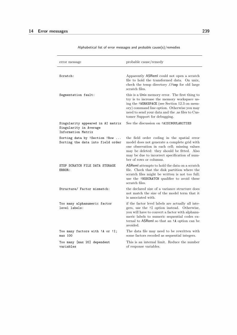
14 Error messages 239

Alphabetical list of error messages and probable cause(s)/remedies

error message probable cause/remedy

Scratch: Apparently ASReml could not open a scratchfile to hold the transformed data. On unix,check the temp directory //tmp for old largescratch files.

Segmentation fault: this is a Unix memory error. The first thing totry is to increase the memory workspace us-ing the !WORKSPACE (see Section 12.3 on mem-ory) command line option. Otherwise you mayneed to send your data and the .as files to Cus-tomer Support for debugging.

Singularity appeared in AI matrix

Singularity in Average

Information Matrix

See the discussion on !AISINGULARITIES

Sorting data by !Section !Row ...

Sorting the data into field order

the field order coding in the spatial errormodel does not generate a complete grid withone observation in each cell; missing valuesmay be deleted: they should be fitted. Alsomay be due to incorrect specification of num-ber of rows or columns.

STOP SCRATCH FILE DATA STORAGE

ERROR:

ASReml attempts to hold the data on a scratchfile. Check that the disk partition where thescratch files might be written is not too full;use the !NOSCRATCH qualifier to avoid thesescratch files.

Structure/ Factor mismatch: the declared size of a variance structure doesnot match the size of the model term that itis associated with.

Too many alphanumeric factor

level labels:

if the factor level labels are actually all inte-gers, use the !I option instead. Otherwise,you will have to convert a factor with alphanu-meric labels to numeric sequential codes ex-ternal to ASReml so that an !A option can beavoided.

Too many factors with !A or !I;

max 100

The data file may need to be rewritten withsome factors recoded as sequential integers.

Too many [max 20] dependent

variables

This is an internal limit. Reduce the numberof response variables.

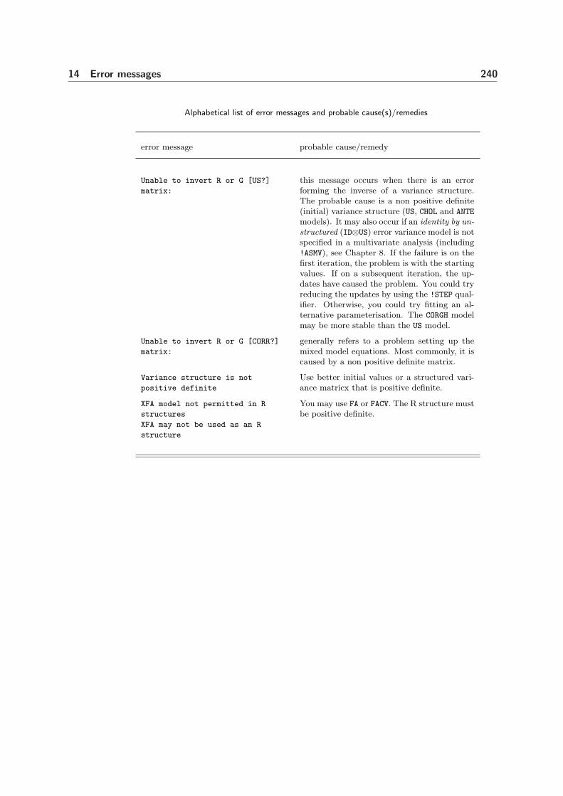
14 Error messages 240

Alphabetical list of error messages and probable cause(s)/remedies

error message probable cause/remedy

Unable to invert R or G [US?]

matrix:

this message occurs when there is an errorforming the inverse of a variance structure.The probable cause is a non positive definite(initial) variance structure (US, CHOL and ANTE

models). It may also occur if an identity by un-structured (ID⊗US) error variance model is notspecified in a multivariate analysis (including!ASMV), see Chapter 8. If the failure is on thefirst iteration, the problem is with the startingvalues. If on a subsequent iteration, the up-dates have caused the problem. You could tryreducing the updates by using the !STEP qual-ifier. Otherwise, you could try fitting an al-ternative parameterisation. The CORGH modelmay be more stable than the US model.

Unable to invert R or G [CORR?]

matrix:

generally refers to a problem setting up themixed model equations. Most commonly, it iscaused by a non positive definite matrix.

Variance structure is not

positive definite

Use better initial values or a structured vari-ance matricx that is positive definite.

XFA model not permitted in R

structures

XFA may not be used as an R

structure

You may use FA or FACV. The R structure mustbe positive definite.

15 Examples

Introduction

Split plot design - Oats

Unbalanced nested design - Rats

Source of variability in unbalanced data - Volts

Balanced repeated measures - Height

Spatial analysis of a field experiment - Barley

Unreplicated early generation variety trial - Wheat

Paired Case-Control study - Rice

Standard analysisA multivariate approachInterpretation of results

Balanced longitudinal data - Oranges

Initial analysesRandom coefficients and cubic smoothing splines

Multivariate animal genetics data - Sheep

Half-sib analysisAnimal model

241

15 Examples 242

15.1 Introduction

In this chapter we present the analysis of a variety of examples. The primaryaim is to illustrate the capabilities of ASReml in the context of analysing realdata sets. We also discuss the output produced by ASReml and indicate whenproblems may occur. Statistical concepts and issues are discussed as necessarybut we stress that the analyses are illustrative, not prescriptive.

15.2 Split plot design - Oats

The first example involves the analysis of a split plot design originally presentedby Yates (1935). The experiment was conducted to assess the effects on yieldof three oat varieties (Golden Rain, Marvellous and Victory) with four levels ofnitrogen application (0, 0.2, 0.4 and 0.6 cwt/acre). The field layout consisted ofsix blocks (labelled I, II, III, IV, V and VI) with three whole-plots per block, eachsplit into four sub-plots. The three varieties were randomly allocated to the threewhole-plots while the four levels of nitrogen application were randomly assignedto the four sub-plots within each whole-plot. The data is presented in Table 15.1.

Table 15.1 A split-plot field trial of oat varieties and nitrogen application

nitrogenblock variety 0.0cwt 0.2cwt 0.4cwt 0.6cwt

Victory 111 130 157 174I GoldenRain 117 114 161 141

Marvellous 105 140 118 156Victory 61 91 97 100

II GoldenRain 70 108 126 149Marvelous 96 124 121 144Victory 68 64 112 86

III GoldenRain 60 102 89 96Marvellous 89 129 132 124Victory 74 89 81 122

IV GoldenRain 64 103 132 133Marvelous 70 89 104 117Victory 62 90 100 116

V GoldenRain 80 82 94 126Marvellous 63 70 109 99Victory 53 74 118 113

VI GoldenRain 89 82 86 104Marvellous 97 99 119 121

A standard analysis of these data recognises the two basic elements inherent inthe experiment. These two aspects are firstly the stratification of the experimentunits, that is the blocks, whole-plots and sub-plots, and secondly, the treatment

15 Examples 243

structure that is superimposed on the experimental material. The latter is ofprime interest, in the presence of stratification. Thus the aim of the analysisis to examine the importance of the treatment effects while accounting for thestratification and restricted randomisation of the treatments to the experimentalunits. The ASReml input file is presented below.

split plot example

blocks 6 # Coded 1...6 in first data field of oats.asd

nitrogen !A 4 # Coded alphabetically

subplots * # Coded 1...4

variety !A 3 # Coded alphabetically

wplots * # Coded 1...3

yield

oats.asd !SKIP 2

yield ~ mu variety nitrogen variety.nitrogen !r blocks blocks.wplots

predict nitrogen # Print table of predicted nitrogen means

predict variety

predict variety nitrogen !SED

The data fields were blocks, wplots, subplots, variety, nitrogen and yield.The first five variables are factors that describe the stratification or experi-ment design and treatments. The standard split plot analysis is achieved byfitting the model terms blocks and blocks.wplots as random effects. Theblocks.wplots.subplots term is not listed in the model because this interac-tion corresponds to the experimental units and is automatically included as theresidual term. The fixed effects include the main effects of both variety andnitrogen and their interaction. The tables of predicted means and associatedstandard errors of differences (SEDs) have been requested. These are reported inthe .pvs file. Abbreviated output is shown below.

Approximate stratum variance decomposition

Stratum Degrees-Freedom Variance Component Coefficients

blocks 5.00 3175.06 12.0 4.0 1.0

blocks.wplots 10.00 601.331 0.0 4.0 1.0

Residual Variance 45.00 177.083 0.0 0.0 1.0

Source Model terms Gamma Component Comp/SE % C

blocks 6 6 1.21116 214.477 1.27 0 P

blocks.wplots 18 18 0.598937 106.062 1.56 0 P

Variance 72 60 1.00000 177.083 4.74 0 P

Analysis of Variance NumDF DenDF F_inc Prob

7 mu 1 5.0 245.14 <.001

4 variety 2 10.0 1.49 0.272

2 nitrogen 3 45.0 37.69 <.001

8 variety.nitrogen 6 45.0 0.30 0.932

15 Examples 244

For simple variance component models such as the above, the default parame-terisation for the variance component parameters is as the ratio to the residualvariance. Thus ASReml prints the variance component ratio and variance com-ponent for each term in the random model in the columns labelled Gamma andComponent respectively.

The analysis of variance (ANOVA) is printed below this summary. The usualdecomposition has three strata, with treatment effects separating into differentstrata as a consequence of the balanced design and the allocation of variety towhole-plots. In this balanced case, it is straightforward to derive the ANOVA

estimates of the stratum variances from the REML estimates of the variancecomponents. That is

blocks stratum variance = 12σ2b + 4σ2

w + σ2 = 3175.06

blocks.wplots stratum variance = 4σ2w + σ2 = 601.331

residual stratum variance = σ2 = 177.083

where σ2b is the blocks variance component, σ2

w is the blocks.wplots componentand σ2 is the residual variance.

The default output for testing fixed effects used by ASReml is a table of so-calledincremental F-statistics. These F-statistics are described in Section 6.12. Thestatistics are simply the appropriate Wald test statistics divided by the number ofestimable effects for that term. In this example there are four terms included inthe summary. The overall mean (denoted by mu) is of no interest for these data.The tests are sequential, that is the effect of each term is assessed by the changein sums of squares achieved by adding the term to the current model, defined bythe model which includes those terms appearing above the current term giventhe variance parameters. For example, the test of nitrogen is calculated fromthe change in sums of squares for the two models mu variety nitrogen and muvariety. No refitting occurs, that is the variance parameters are held constantat the REML estimates obtained from the currently specified fixed model.

The incremental Wald statistics have an asymptotic χ2 distribution, with degreesof freedom (df) given by the number of estimable effects (the number in the DFcolumn). In this example, the incremental F-statistics are numerically the same asthe ANOVA F-statistics, and ASReml has calculated the appropriate denominatordf for testing fixed effects. This is a simple problem for balanced designs, suchas the split plot design, but it is not straightforward to determine the relevantdenominator df in unbalanced designs, such as the rat data set described in thenext section.

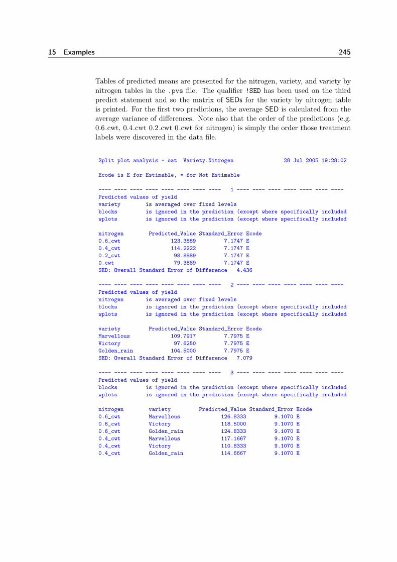
15 Examples 245

Tables of predicted means are presented for the nitrogen, variety, and variety bynitrogen tables in the .pvs file. The qualifier !SED has been used on the thirdpredict statement and so the matrix of SEDs for the variety by nitrogen tableis printed. For the first two predictions, the average SED is calculated from theaverage variance of differences. Note also that the order of the predictions (e.g.0.6 cwt, 0.4 cwt 0.2 cwt 0 cwt for nitrogen) is simply the order those treatmentlabels were discovered in the data file.

Split plot analysis - oat Variety.Nitrogen 28 Jul 2005 19:28:02

Ecode is E for Estimable, * for Not Estimable

---- ---- ---- ---- ---- ---- ---- ---- 1 ---- ---- ---- ---- ---- ---- ----

Predicted values of yield

variety is averaged over fixed levels

blocks is ignored in the prediction (except where specifically included

wplots is ignored in the prediction (except where specifically included

nitrogen Predicted_Value Standard_Error Ecode

0.6_cwt 123.3889 7.1747 E

0.4_cwt 114.2222 7.1747 E

0.2_cwt 98.8889 7.1747 E

0_cwt 79.3889 7.1747 E

SED: Overall Standard Error of Difference 4.436

---- ---- ---- ---- ---- ---- ---- ---- 2 ---- ---- ---- ---- ---- ---- ----

Predicted values of yield

nitrogen is averaged over fixed levels

blocks is ignored in the prediction (except where specifically included

wplots is ignored in the prediction (except where specifically included

variety Predicted_Value Standard_Error Ecode

Marvellous 109.7917 7.7975 E

Victory 97.6250 7.7975 E

Golden_rain 104.5000 7.7975 E

SED: Overall Standard Error of Difference 7.079

---- ---- ---- ---- ---- ---- ---- ---- 3 ---- ---- ---- ---- ---- ---- ----

Predicted values of yield

blocks is ignored in the prediction (except where specifically included

wplots is ignored in the prediction (except where specifically included

nitrogen variety Predicted_Value Standard_Error Ecode

0.6_cwt Marvellous 126.8333 9.1070 E

0.6_cwt Victory 118.5000 9.1070 E

0.6_cwt Golden_rain 124.8333 9.1070 E

0.4_cwt Marvellous 117.1667 9.1070 E

0.4_cwt Victory 110.8333 9.1070 E

0.4_cwt Golden_rain 114.6667 9.1070 E

15 Examples 246

0.2_cwt Marvellous 108.5000 9.1070 E

0.2_cwt Victory 89.6667 9.1070 E

0.2_cwt Golden_rain 98.5000 9.1070 E

0_cwt Marvellous 86.6667 9.1070 E

0_cwt Victory 71.5000 9.1070 E

0_cwt Golden_rain 80.0000 9.1070 E

Predicted values with SED(PV)

126.833

118.500 9.71503

124.833 9.71503 9.71503

117.167 7.68295 9.71503 9.71503

110.833 9.71503 7.68295 9.71503 9.71503

114.667 9.71503 9.71503 7.68295 9.71503

9.71503

108.500 7.68295 9.71503 9.71503 7.68295

9.71503 9.71503

89.6667 9.71503 7.68295 9.71503 9.71503

7.68295 9.71503 9.71503

98.5000 9.71503 9.71503 7.68295 9.71503

9.71503 7.68295 9.71503 9.71503

86.6667 7.68295 9.71503 9.71503 7.68295

9.71503 9.71503 7.68295 9.71503 9.71503

71.5000 9.71503 7.68295 9.71503 9.71503

7.68295 9.71503 9.71503 7.68295 9.71503

9.71503

80.0000 9.71503 9.71503 7.68295 9.71503

9.71503 7.68295 9.71503 9.71503 7.68295

9.71503 9.71503

SED: Standard Error of Difference: Min 7.6830 Mean 9.1608 Max 9.7150

15.3 Unbalanced nested design - Rats

The second example we consider is a data set which illustrates some furtheraspects of testing fixed effects in linear mixed models. This example differs fromthe split plot example, as it is unbalanced and so more care is required in assessingthe significance of fixed effects.

The experiment was reported by Dempster et al. (1984) and was designed tocompare the effect of three doses of an experimental compound (control, lowand high) on the maternal performance of rats. Thirty female rats (dams) wererandomly split into three groups of 10 and each group randomly assigned to thethree different doses. All pups in each litter were weighed. The litters differed intotal size and in the numbers of males and females. Thus the additional covariate,littersize was included in the analysis. The differential effect of the compound

15 Examples 247

on male and female pups was also of interest. Three litters had to be droppedfrom experiment, which meant that one dose had only 7 dams. The analysismust account for the presence of between dam variation, but must also recognisethe stratification of the experimental units (pups within litters) and that dosesand littersize belong to the dam stratum. Table 15.2 presents an indicative AOV

decomposition for this experiment.

Table 15.2 Rat data: AOV decomposition

stratum decomposition type df or ne

constant 1 F 1dams

dose F 2littersize F 1dam R 27

dams.pupssex F 1dose.sex F 2

error R

The dose and littersize effects are tested against the residual dam variation, whilethe remaining effects are tested against the residual within litter variation. TheASReml input to achieve this analysis is presented below.

Rats example

dose 3 !A

sex 2 !A

littersize

dam 27

pup 18

weight

rats.asd !DOPATH 1 # Change DOPATH argument to select each PATH

!PATH 1

weight ~ mu littersize dose sex dose.sex !r dam

!PATH 2

weight ~ mu out(66) littersize dose sex dose.sex !r dam

!PATH 3

weight ~ mu littersize dose sex !r dam

!PATH 4

weight ~ mu littersize dose sex

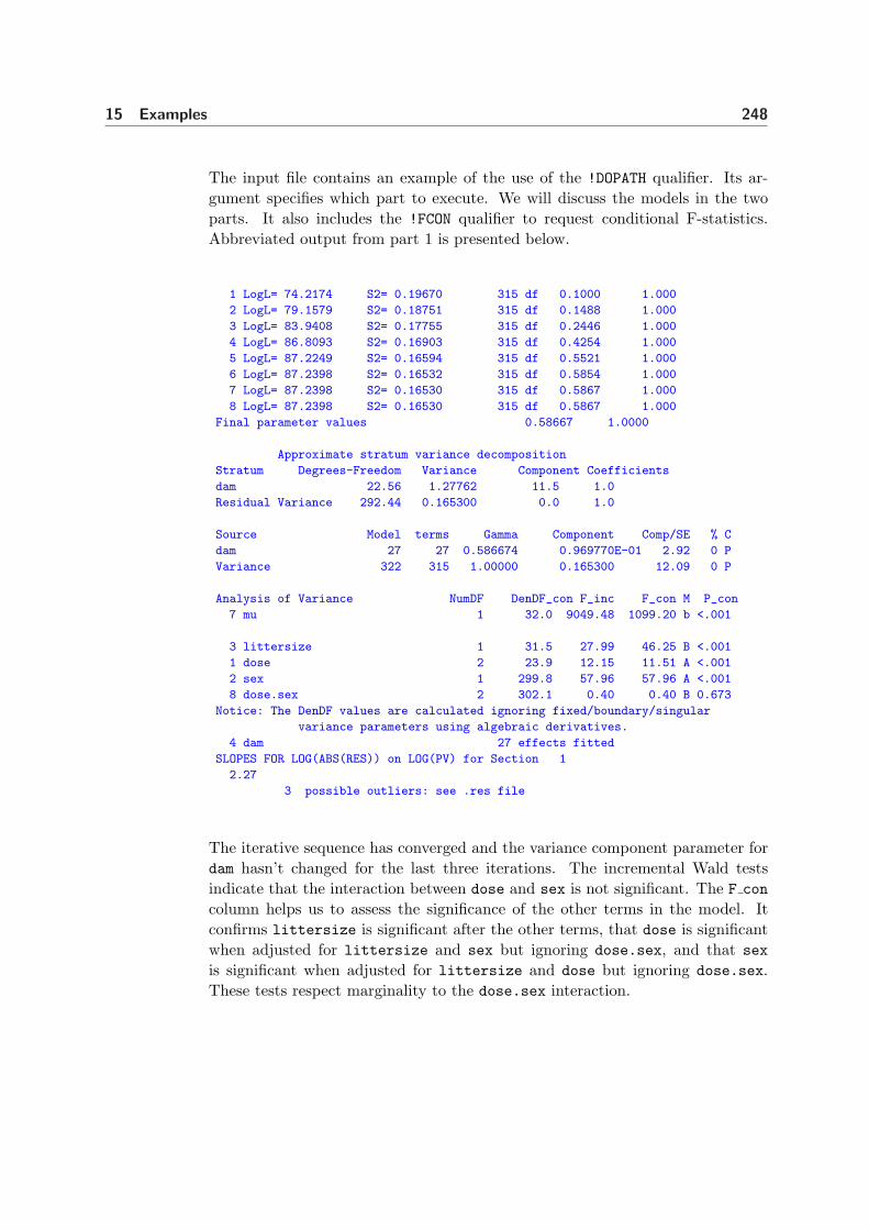
15 Examples 248

The input file contains an example of the use of the !DOPATH qualifier. Its ar-gument specifies which part to execute. We will discuss the models in the twoparts. It also includes the !FCON qualifier to request conditional F-statistics.Abbreviated output from part 1 is presented below.

1 LogL= 74.2174 S2= 0.19670 315 df 0.1000 1.000

2 LogL= 79.1579 S2= 0.18751 315 df 0.1488 1.000

3 LogL= 83.9408 S2= 0.17755 315 df 0.2446 1.000

4 LogL= 86.8093 S2= 0.16903 315 df 0.4254 1.000

5 LogL= 87.2249 S2= 0.16594 315 df 0.5521 1.000

6 LogL= 87.2398 S2= 0.16532 315 df 0.5854 1.000

7 LogL= 87.2398 S2= 0.16530 315 df 0.5867 1.000

8 LogL= 87.2398 S2= 0.16530 315 df 0.5867 1.000

Final parameter values 0.58667 1.0000

Approximate stratum variance decomposition

Stratum Degrees-Freedom Variance Component Coefficients

dam 22.56 1.27762 11.5 1.0

Residual Variance 292.44 0.165300 0.0 1.0

Source Model terms Gamma Component Comp/SE % C

dam 27 27 0.586674 0.969770E-01 2.92 0 P

Variance 322 315 1.00000 0.165300 12.09 0 P

Analysis of Variance NumDF DenDF_con F_inc F_con M P_con

7 mu 1 32.0 9049.48 1099.20 b <.001

3 littersize 1 31.5 27.99 46.25 B <.001

1 dose 2 23.9 12.15 11.51 A <.001

2 sex 1 299.8 57.96 57.96 A <.001

8 dose.sex 2 302.1 0.40 0.40 B 0.673

Notice: The DenDF values are calculated ignoring fixed/boundary/singular

variance parameters using algebraic derivatives.

4 dam 27 effects fitted

SLOPES FOR LOG(ABS(RES)) on LOG(PV) for Section 1

2.27

3 possible outliers: see .res file

The iterative sequence has converged and the variance component parameter fordam hasn’t changed for the last three iterations. The incremental Wald testsindicate that the interaction between dose and sex is not significant. The F concolumn helps us to assess the significance of the other terms in the model. Itconfirms littersize is significant after the other terms, that dose is significantwhen adjusted for littersize and sex but ignoring dose.sex, and that sexis significant when adjusted for littersize and dose but ignoring dose.sex.These tests respect marginality to the dose.sex interaction.

15 Examples 249

We also note the comment 3 possible outliers: see .res file. Checkingthe .res file, we discover unit 66 has a standardised residual of -8.80 (see Fig-ure 15.1). The weight of this female rat, within litter 9 is only 3.68, compared toweights of 7.26 and 6.58 for two other female sibling pups. This weight appearserroneous, but without knowledge of the actual experiment we retain the obser-vation in the following. However, part 2 shows one way of ’dropping’ unit 66 byfitting an effect for it with out(66).

Rats example Residuals vs Fitted values Residuals (Y) −3.02: 1.22 Fitted values (X) 5.04: 7.63

Figure 15.1 Residual plot for the rat data

We refit the model without the dose.sex term. Note that the variance parame-ters are re-estimated, though there is little change from the previous analysis.

Source Model terms Gamma Component Comp/SE % C

dam 27 27 0.595157 0.979179E-01 2.93 0 P

Variance 322 317 1.00000 0.164524 12.13 0 P

Analysis of Variance NumDF DenDF_con F_inc F_con M P_con

7 mu 1 32.0 8981.48 1093.05 . <.001

3 littersize 1 31.4 27.85 46.43 A <.001

1 dose 2 24.0 12.05 11.42 A <.001

2 sex 1 301.7 58.27 58.27 A <.001

Part 4 shows what happens if we (wrongly) drop dam from this model. Even ifa random term is not ’significant’, it should not be dropped from the model if itrepresents a strata of the design as in this case.

15 Examples 250

Source Model terms Gamma Component Comp/SE % C

Variance 322 317 1.00000 0.253182 12.59 0 P

Analysis of Variance NumDF DenDF_con F_inc F_con M P_con

7 mu 1 317.0 47077.31 3309.42 . <.001

3 littersize 1 317.0 68.48 146.50 A <.001

1 dose 2 317.0 60.99 58.43 A <.001

2 sex 1 317.0 24.52 24.52 A <.001

15.4 Source of variability in unbalanced data - Volts

In this example we illustrate an analysis of unbalanced data in which the mainaim is to determine the sources of variation rather than assess the significance ofimposed treatments. The data are taken from Cox and Snell (1981) and involve anexperiment to examine the variability in the production of car voltage regulators.Standard production of regulators involves two steps. Regulators are taken fromthe production line to a setting station and adjusted to operate within a specifiedvoltage range. From the setting station the regulator is then passed to a testingstation where it is tested and returned if outside the required range.

The voltage of 64 regulators was set at 10 setting stations (setstat); between4 and 8 regulators were set at each station. The regulators were each tested atfour testing stations (teststat). The ASReml input file is presented below.

Voltage data

teststat 4 # 4 testing stations tested each regulator

setstat !A # 10 setting stations each set 4-8 regulators

regulatr 8 # regulators numbered within setting stations

voltage

voltage.asd !skip 1

voltage ~ mu !r setstat setstat.regulatr teststat setstat.teststat

0 0 0

The factor regulatr numbers the regulators within each setting station. Thusthe term setstat.regulatr allows for differential effects of each regulator, whilethe other terms examine the effects of the setting and testing stations and possibleinteraction. The abbreviated output is given below

LogL= 188.604 S2= 0.67074E-01 255 df

LogL= 199.530 S2= 0.59303E-01 255 df

15 Examples 251

LogL= 203.007 S2= 0.52814E-01 255 df

LogL= 203.240 S2= 0.51278E-01 255 df

LogL= 203.242 S2= 0.51141E-01 255 df

LogL= 203.242 S2= 0.51140E-01 255 df

Source Model terms Gamma Component Comp/SE % C

setstat 10 10 0.233418 0.119371E-01 1.35 0 P

setstat.regulatr 80 64 0.601817 0.307771E-01 3.64 0 P

teststat 4 4 0.642752E-01 0.328706E-02 0.98 0 P

setstat.teststat 40 40 0.100000E-08 0.511404E-10 0.00 0 B

Variance 256 255 1.00000 0.511404E-01 9.72 0 P

Warning: Code B - fixed at a boundary (!GP) F - fixed by user

? - liable to change from P to B P - positive definite

C - Constrained by user (!VCC) U - unbounded

S - Singular Information matrix

The convergence criteria has been satisfied after six iterations. A warning messagein printed below the summary of the variance components because the variancecomponent for the setstat.teststat term has been fixed near the boundary.The default constraint for variance components (!GP) is to ensure that the REML

estimate remains positive. Under this constraint, if an update for any variancecomponent results in a negative value then ASReml sets that variance componentto a small positive value. If this occurs in subsequent iterations the parameter isfixed to a small positive value and the code B replaces P in the C column of thesummary table. The default constraint can be overridden using the !GU qualifier,but it is not generally recommended for standard analyses.

Figure 15.2 presents the residual plot which indicates two unusual data values.These values are successive observations, namely observation 210 and 211, beingtesting stations 2 and 3 for setting station 9(J), regulator 2. These observa-tions will not be dropped from the following analyses for consistency with otheranalyses conducted by Cox and Snell (1981) and in the GENSTAT manual.

The REML log-likelihood from the model without the setstat.teststat termwas 203.242, the same as the REML log-likelihood for the previous model. Ta-ble 15.3 presents a summary of the REML log-likelihood ratio for the remainingterms in the model. The summary of the ASReml output for the current model isgiven below. The column labelled Comp/SE is printed by ASReml to give a guideas to the significance of the variance component for each term in the model. Thestatistic is simply the REML estimate of the variance component divided by thesquare root of the diagonal element (for each component) of the inverse of theaverage information matrix. The diagonal elements of the expected (not the av-erage) information matrix are the asymptotic variances of the REML estimates

15 Examples 252

ltage example 5−3−6 from the GENSTAT REML manual Residuals vs Fitted valu Residuals (Y) −1.08: 1.45 Fitted values (X) 15.56: 16.81

Figure 15.2 Residual plot for the voltage data

of the variance parameters. These Comp/SE statistics cannot be used to test thenull hypothesis that the variance component is zero. If we had used this crudemeasure then the conclusions would have been inconsistent with the conclusionsobtained from the REML log-likelihood ratio (see Table 15.3).

Source Model terms Gamma Component Comp/SE % C

setstat 10 10 0.233417 0.119370E-01 1.35 0 P

setstat.regulatr 80 64 0.601817 0.307771E-01 3.64 0 P

teststat 4 4 0.642752E-01 0.328705E-02 0.98 0 P

Variance 256 255 1.00000 0.511402E-01 9.72 0 P

Table 15.3: REML log-likelihood ratio for the variance components in the voltagedata

REML −2×terms log-likelihood difference P-value

− setstat 200.31 5.864 .0077− setstat.regulatr 184.15 38.19 .0000− teststat 199.71 7.064 .0039

15 Examples 253

15.5 Balanced repeated measures - Height

The data for this example is taken from the GENSTAT manual. It consists ofa total of 5 measurements of height (cm) taken on 14 plants. The 14 plantswere either diseased or healthy and were arranged in a glasshouse in a completelyrandom design. The heights were measured 1, 3, 5, 7 and 10 weeks after theplants were placed in the glasshouse. There were 7 plants in each treatment. Thedata are depicted in Figure 15.3 obtained by qualifier line!Y y1 !G tmt !JOINin the following multivariate ASReml job.

This is plant data multivariate Y=y1 X=Traits G=tmt

1 2

Y−axis: 21.0000 130.5000 X−axis: 0.5000 5.5000

Figure 15.3 Trellis plot of the height for each of 14 plants

In the following we illustrate how various repeated measures analyses can beconducted in ASReml. For these analyses it is convenient to arrange the datain a multivariate form, with 7 fields representing the plant number, treatmentidentification and the 5 heights. The ASReml input file, up to the specificationof the R structure is

This is plant data multivariate

tmt !A # Diseased Healthy

plant 14

y1 y3 y5 y7 y10

grass.asd !skip 1 !ASUV

15 Examples 254

The focus is modelling of the error variance for the data. Specifically we fit themultivariate regression model given by

Y = DT + E (15.1)

where Y 14×5 is the matrix of heights, D14×2 is the design matrix, T 2×5 is thematrix of fixed effects and E14×5 is the matrix of errors. The heights taken onthe same plants will be correlated and so we assume that

var (vec(E)) = I14 ⊗Σ (15.2)

where Σ5×5 is a symmetric positive definite matrix.

The variance models used for Σ are given in Table 15.4. These represent somecommonly used models for the analysis of repeated measures data (see Wolfinger,1986). The variance models are fitted by changing the last four lines of the inputfile. The sequence of commands for the first model fitted is

y1 y3 y5 y7 y10 ~ Trait tmt Tr.tmt !r units

1 2 0

14

Trait

Table 15.4 Summary of variance models fitted to the plant data

number of REMLmodel parameters log-likelihood BIC

Uniform 2 -196.88 401.95Power 2 -182.98 374.15Heterogeneous Power 6 -171.50 367.57Antedependence (order 1) 9 -160.37 357.51Unstructured 15 -158.04 377.50

The split plot in time model can be fitted in two ways, either by fitting a unitsterm plus an independent residual as above, or by specifying a CORU variancemodel for the R-structure as follows

y1 y3 y5 y7 y10 ~ Trait tmt Tr.tmt

1 2 0

14

Trait 0 CORU .5

15 Examples 255

The two forms for Σ are given by

Σ = σ21J + σ2

2I, unitsΣ = σ2

eI + σ2eρ(J − I), CORU

(15.3)

It follows that

σ2e = σ2

1 + σ22

ρ = σ21

σ21+σ2

2

(15.4)

Portions of the two outputs are given below. The REML log-likelihoods for thetwo models are the same and it is easy to verify that the REML estimates ofthe variance parameters satisfy (15.4), viz. σ2

e = 286.310 ≈ 159.858 + 126.528 =286.386; 159.858/286.386 = 0.558191.#

# !r units

#

LogL=-204.593 S2= 224.61 60 df 0.1000 1.000

LogL=-201.233 S2= 186.52 60 df 0.2339 1.000

LogL=-198.453 S2= 155.09 60 df 0.4870 1.000

LogL=-197.041 S2= 133.85 60 df 0.9339 1.000

LogL=-196.881 S2= 127.56 60 df 1.204 1.000

LogL=-196.877 S2= 126.53 60 df 1.261 1.000

Final parameter values 1.2634 1.0000

Source Model terms Gamma Component Comp/SE % C

units 14 14 1.26342 159.858 2.11 0 P

Variance 70 60 1.00000 126.528 4.90 0 P

#

# CORU

#

LogL=-196.975 S2= 264.10 60 df 1.000 0.5000

LogL=-196.924 S2= 270.14 60 df 1.000 0.5178

LogL=-196.886 S2= 278.58 60 df 1.000 0.5400

LogL=-196.877 S2= 286.23 60 df 1.000 0.5580

LogL=-196.877 S2= 286.31 60 df 1.000 0.5582

Final parameter values 1.0000 0.55819

Source Model terms Gamma Component Comp/SE % C

Variance 70 60 1.00000 286.310 3.65 0 P

Residual CORRelat 5 0.558191 0.558191 4.28 0 U

A more realistic model for repeated measures data would allow the correlationsto decrease as the lag increases such as occurs with the first order autoregressivemodel. However, since the heights are not measured at equally spaced time pointswe use the EXP model. The correlation function is given by

ρ(u) = φu

where u is the time lag is weeks. The coding for this is

15 Examples 256

y1 y3 y5 y7 y10 ~ Trait tmt Tr.tmt

1 2 0 # One error structure in two dimensions

14 # Outer dimension: 14 plants

Tr 0 EXP .5

1 3 5 7 10 # Time coordinates

A portion of the output is

LogL=-183.734 S2= 435.58 60 df 1.000 0.9500

LogL=-183.255 S2= 370.40 60 df 1.000 0.9388

LogL=-183.010 S2= 321.50 60 df 1.000 0.9260

LogL=-182.980 S2= 298.84 60 df 1.000 0.9179

LogL=-182.979 S2= 302.02 60 df 1.000 0.9192

Final parameter values 1.0000 0.91897

Source Model terms Gamma Component Comp/SE % C

Variance 70 60 1.00000 302.021 3.11 0 P

Residual POW-EXP 5 0.918971 0.918971 29.53 0 U

When fitting power models be careful to ensure the scale of the defining variate,here time, does not result in an estimate of φ too close to 1. For example, use ofdays in this example would result in an estimate for φ of about .993.

Residuals plotted against Row and Column position: 1Range: −45.11 34.86

Figure 15.4 Residual plots for the EXP variance model for the plant data

The residual plot from this analysis is presented in Figure 15.4. This suggestsincreasing variance over time. This can be modelled by using the EXPH model,

15 Examples 257

which models Σ byΣ = D0.5CD0.5

where D is a diagonal matrix of variances and C is a correlation matrix withelements given by cij = φ|ti−tj |. The coding for this is

y1 y3 y5 y7 y10 ~ Trait tmt Tr.tmt

1 2 0

14 !S2==1

Tr 0 EXPH .5 100 200 300 300 300

1 3 5 7 10

Note that it is necessary to fix the scale parameter to 1 (!S2==1) to ensure thatthe elements of D are identifiable. Abbreviated output from this analysis is

1 LogL=-195.598 S2= 1.0000 60 df : 1 components constrained

2 LogL=-179.036 S2= 1.0000 60 df

3 LogL=-175.483 S2= 1.0000 60 df

4 LogL=-173.128 S2= 1.0000 60 df

5 LogL=-171.980 S2= 1.0000 60 df

6 LogL=-171.615 S2= 1.0000 60 df

7 LogL=-171.527 S2= 1.0000 60 df

8 LogL=-171.504 S2= 1.0000 60 df

9 LogL=-171.498 S2= 1.0000 60 df

10 LogL=-171.496 S2= 1.0000 60 df

Source Model terms Gamma Component Comp/SE % C

Residual POW-EXP 5 0.906917 0.906917 21.89 0 U

Residual POW-EXP 5 60.9599 60.9599 2.12 0 U

Residual POW-EXP 5 72.9904 72.9904 1.99 0 U

Residual POW-EXP 5 309.259 309.259 2.22 0 U

Residual POW-EXP 5 436.380 436.380 2.52 0 U

Residual POW-EXP 5 382.369 382.369 2.74 0 U

Covariance/Variance/Correlation Matrix POWER

61.11 0.8227 0.6769 0.5569 0.4156

54.88 72.80 0.8227 0.6769 0.5051

93.12 123.5 309.7 0.8227 0.6140

91.02 120.7 302.7 437.1 0.7462

63.57 84.34 211.4 305.3 382.9

Analysis of Variance DF F_inc

8 Trait 5 127.95

1 tmt 1 0.00

9 Tr.tmt 4 4.75

The last two models we fit are the antedependence model of order 1 and theunstructured model. These require, as starting values the lower triangle of thefull variance matrix. We use the REML estimate of Σ from the heterogeneous

15 Examples 258

power model shown in the previous output. The antedependence model modelsΣ by the inverse cholesky decomposition

Σ−1 = UDU ′

where D is a diagonal matrix and U is a unit upper triangular matrix. Foran antedependence model of order q, then uij = 0 for j > i + q − 1. Theantedependence model of order 1 has 9 parameters for these data, 5 in D and 4in U . The input is given by

y1 y3 y5 y7 y10 ~ Trait tmt Tr.tmt

1 2 0

14 !S2==1

Tr 0 ANTE

60.16

54.65 73.65

91.50 123.3 306.4

89.17 120.2 298.6 431.8

62.21 83.85 208.3 301.2 379.8

The abbreviated output file is

1 LogL=-171.501 S2= 1.0000 60 df

2 LogL=-170.097 S2= 1.0000 60 df

3 LogL=-166.085 S2= 1.0000 60 df

4 LogL=-161.335 S2= 1.0000 60 df

5 LogL=-160.407 S2= 1.0000 60 df

6 LogL=-160.370 S2= 1.0000 60 df

7 LogL=-160.369 S2= 1.0000 60 df

Source Model terms Gamma Component Comp/SE % C

Residual ANTE=UDU 1 0.268657E-01 0.268657E-01 2.44 0 U

Residual ANTE=UDU 1 -0.628413 -0.628413 -2.55 0 U

Residual ANTE=UDU 2 0.372801E-01 0.372801E-01 2.41 0 U

Residual ANTE=UDU 2 -1.49108 -1.49108 -2.54 0 U

Residual ANTE=UDU 3 0.599632E-02 0.599632E-02 2.43 0 U

Residual ANTE=UDU 3 -1.28041 -1.28041 -6.19 0 U

Residual ANTE=UDU 4 0.789713E-02 0.789713E-02 2.44 0 U

Residual ANTE=UDU 4 -0.967815 -0.967815 -15.40 0 U

Residual ANTE=UDU 5 0.390635E-01 0.390635E-01 2.45 0 U

Covariance/Variance/Correlation Matrix ANTE=UDU’

37.20 0.5946 0.3549 0.3114 0.3040

23.38 41.55 0.5968 0.5237 0.5112

34.83 61.89 258.9 0.8775 0.8565

44.58 79.22 331.4 550.8 0.9761

43.14 76.67 320.7 533.0 541.4

Analysis of Variance DF F_inc

8 Trait 5 188.84

15 Examples 259

1 tmt 1 4.14

9 Tr.tmt 4 3.91

The iterative sequence converged and the antedependence parameter estimatesare printed columnwise by time, the column of U and the element of D. I.e.

D = diag

0.02690.03730.00600.00790.0391

,U =

1 −0.6284 0 0 00 1 −1.4911 0 00 0 1 −1.2804 00 0 0 1 −0.96780 0 0 0 1

.

Finally the input and output files for the unstructured model are presented below.The REML estimate of Σ from the ANTE model is used to provide starting values.

###########

#input

###########

y1 y3 y5 y7 y10 ~ Trait tmt Tr.tmt

1 2 0

14 !S2==1

Tr 0 US

37.20

23.38 41.55

34.83 61.89 258.9

44.58 79.22 331.4 550.8

43.14 76.67 320.7 533.0 541.4

############

# output

############

1 LogL=-160.368 S2= 1.0000 60 df

2 LogL=-159.027 S2= 1.0000 60 df

3 LogL=-158.247 S2= 1.0000 60 df

4 LogL=-158.040 S2= 1.0000 60 df

5 LogL=-158.036 S2= 1.0000 60 df

Source Model terms Gamma Component Comp/SE % C

Residual US=UnStr 1 37.2262 37.2262 2.45 0 U

Residual US=UnStr 1 23.3935 23.3935 1.77 0 U

Residual US=UnStr 2 41.5195 41.5195 2.45 0 U

Residual US=UnStr 1 51.6524 51.6524 1.61 0 U

Residual US=UnStr 2 61.9169 61.9169 1.78 0 U

Residual US=UnStr 3 259.121 259.121 2.45 0 U

Residual US=UnStr 1 70.8113 70.8113 1.54 0 U

15 Examples 260

Residual US=UnStr 2 57.6146 57.6146 1.23 0 U

Residual US=UnStr 3 331.807 331.807 2.29 0 U

Residual US=UnStr 4 551.507 551.507 2.45 0 U

Residual US=UnStr 1 73.7857 73.7857 1.60 0 U

Residual US=UnStr 2 62.5691 62.5691 1.33 0 U

Residual US=UnStr 3 330.851 330.851 2.29 0 U

Residual US=UnStr 4 533.756 533.756 2.42 0 U

Residual US=UnStr 5 542.175 542.175 2.45 0 U

Covariance/Variance/Correlation Matrix US=UnStructu

37.23 0.5950 0.5259 0.4942 0.5194

23.39 41.52 0.5969 0.3807 0.4170

51.65 61.92 259.1 0.8777 0.8827

70.81 57.61 331.8 551.5 0.9761

73.79 62.57 330.9 533.8 542.2

The antedependence model of order 1 is clearly more parsimonious than theunstructured model. Table 15.5 presents the incremental Wald tests for each ofthe variance models. There is a surprising level of discrepancy between modelsfor the Wald tests. The main effect of treatment is significant for the uniform,power and antedependence models.

Table 15.5: Summary of Wald test for fixed effects for variance models fitted to theplant data

treatment treatment.timemodel (df=1) (df=4)

Uniform 9.41 5.10Power 6.86 6.13Heterogeneous power 0.00 4.81Antedependence (order 1) 4.14 3.96Unstructured 1.71 4.46

15 Examples 261

15.6 Spatial analysis of a field experiment - Barley

In this section we illustrate the ASReml syntax for performing spatial and in-complete block analysis of a field experiment. There has been a large amountof interest in developing techniques for the analysis of spatial data both in thecontext of field experiments and geostatistical data (see for example, Cullis andGleeson, 1991; Cressie, 1991; Gilmour et al., 1997). This example illustrates theanalysis of ’so-called’ regular spatial data, in which the data is observed on alattice or regular grid. This is typical of most small plot designed field exper-iments. Spatial data is often irregularly spaced, either by design or because ofthe observational nature of the study. The techniques we present in the followingcan be extended for the analysis of irregularly spaced spatial data, though, largerspatial data sets may be computationally challenging, depending on the degreeof irregularity or models fitted.

The data we consider is taken from Gilmour et al. (1995) and involves a fieldexperiment designed to compare the performance of 25 varieties of barley. Theexperiment was conducted at Slate Hall Farm, UK in 1976, and was designed asa balanced lattice square with replicates laid out as shown in Table 15.6. Thedata fields were Rep, RowBlk, ColBlk, row, column and yield. Lattice rowand column numbering is typically within replicates and so the terms specified inthe linear model to account for the lattice row and lattice column effects wouldbe Rep.latticerow Rep.latticecolumn. However, in this example lattice rowsand columns are both numbered from 1 to 30 across replicates (see Table 15.6).The terms in the linear model are therefore simply RowBlk ColBlk. Additionalfields row and column indicate the spatial layout of the plots.

The ASReml input file is presented below. Three models have been fitted to thesedata. The lattice analysis is included for comparison in PATH 3. In PATH 1 weuse the separable first order autoregressive model to model the variance structureof the plot errors. Gilmour et al. (1997) suggest this is often a useful model tocommence the spatial modelling process. The form of the variance matrix for theplot errors (R structure) is given by

σ2Σ = σ2(Σc ⊗Σr) (15.5)

where Σc and Σr are 15 × 15 and 10 × 10 matrix functions of the column (φc)and row (φr) autoregressive parameters respectively.

Gilmour et al. (1997) recommend revision of the current spatial model basedon the use of diagnostics such as the sample variogram of the residuals (from

15 Examples 262

the current model). This diagnostic and a summary of row and column residualtrends are produced by default with graphical versions of ASReml when a spatialmodel has been fitted to the errors. It can be suppressed, by the use of the -noption on the command line. We have produced the following plots by use of the-g22 option.

Table 15.6 Field layout of Slate Hall Farm experiment

Column - Replicate levelsRow 1 2 3 4 5 6 7 8 9 10 11 12 13 14 151 1 1 1 1 1 2 2 2 2 2 3 3 3 3 32 1 1 1 1 1 2 2 2 2 2 3 3 3 3 33 1 1 1 1 1 2 2 2 2 2 3 3 3 3 34 1 1 1 1 1 2 2 2 2 2 3 3 3 3 35 1 1 1 1 1 2 2 2 2 2 3 3 3 3 36 4 4 4 4 4 5 5 5 5 5 6 6 6 6 67 4 4 4 4 4 5 5 5 5 5 6 6 6 6 68 4 4 4 4 4 5 5 5 5 5 6 6 6 6 69 4 4 4 4 4 5 5 5 5 5 6 6 6 6 610 4 4 4 4 4 5 5 5 5 5 6 6 6 6 6

Column - Rowblk levelsRow 1 2 3 4 5 6 7 8 9 10 11 12 13 14 151 1 1 1 1 1 11 11 11 11 11 21 21 21 21 212 2 2 2 2 2 12 12 12 12 12 22 22 22 22 223 3 3 3 3 3 13 13 13 13 13 23 23 23 23 234 4 4 4 4 4 14 14 14 14 14 24 24 24 24 245 5 5 5 5 5 15 15 15 15 15 25 25 25 25 256 6 6 6 6 6 16 16 16 16 16 26 26 26 26 267 7 7 7 7 7 17 17 17 17 17 27 27 27 27 278 8 8 8 8 8 18 18 18 18 18 28 28 28 28 289 9 9 9 9 9 19 19 19 19 19 29 29 29 29 2910 10 10 10 10 10 20 20 20 20 20 30 30 30 30 30

Column - Colblk levelsRow 1 2 3 4 5 6 7 8 9 10 11 12 13 14 151 1 2 3 4 5 6 7 8 9 10 11 12 13 14 152 1 2 3 4 5 6 7 8 9 10 11 12 13 14 153 1 2 3 4 5 6 7 8 9 10 11 12 13 14 154 1 2 3 4 5 6 7 8 9 10 11 12 13 14 155 1 2 3 4 5 6 7 8 9 10 11 12 13 14 156 16 17 18 19 20 21 22 23 24 25 26 27 28 29 307 16 17 18 19 20 21 22 23 24 25 26 27 28 29 308 16 17 18 19 20 21 22 23 24 25 26 27 28 29 309 16 17 18 19 20 21 22 23 24 25 26 27 28 29 3010 16 17 18 19 20 21 22 23 24 25 26 27 28 29 30

Slate Hall example

Rep 6 # Six replicates of 5x5 plots in 2x3 arrangement

RowBlk 30 # Rows within replicates numbered across replicates

ColBlk 30 # Columns within replicates numbered across replicates

row 10 # Field row

column 15 # Field column

15 Examples 263

variety 25

yield

barley.asd !skip 1 !DOPATH 1

!PATH 1 # AR1 x AR1

y ~ mu var

predict var

1 2

15 column AR1 0.1 # Second field is specified so ASReml can sort

10 row AR1 0.1 # records properly into field order

!PATH 2 # AR1 x AR1 + units

y ~ mu var !r units

predict var

1 2

15 column AR1 0.1

10 row AR1 0.1

!PATH 3 # incomplete blocks

y ~ mu var !r Rep Rowblk Colblk

predict var

Abbreviated ASReml output file is presented below. The iterative sequence hasconverged to column and row correlation parameters of (.68377,.45859) respec-tively. The plot size and orientation is not known and so it is not possible toascertain whether these values are spatially sensible. It is generally found thatthe closer the plot centroids, the higher the spatial correlation. This is not alwaysthe case and if the highest between plot correlation relates to the larger spatialdistance then this may suggest the presence of extraneous variation (see Gilmouret al., 1997), for example. Figure 15.5 presents a plot of the sample variogramof the residuals from this model. The plot appears in reasonable agreement withthe model.

The next model includes a measurement error or nugget effect component. Thatis the variance model for the plot errors is now given by

σ2Σ = σ2(Σc ⊗Σr) + ψI150 (15.6)

where ψ is the ratio of nugget variance to error variance (σ2). The abbreviatedoutput for this model is given below. There is a significant improvement in theREML log-likelihood with the inclusion of the nugget effect (see Table 15.7).

# AR1 x AR1

#

1 LogL=-739.681 S2= 36034. 125 df 1.000 0.1000 0.1000

15 Examples 264

Slate Hall example f1 1 Variogram of residuals 26 Aug 2002 17:08:51

0

1.569649

Outer displacement Inner displacement

Figure 15.5: Sample variogram of the residuals from the AR1×AR1 model for theSlate Hall data

2 LogL=-714.340 S2= 28109. 125 df 1.000 0.4049 0.1870

3 LogL=-703.338 S2= 29914. 125 df 1.000 0.5737 0.3122

4 LogL=-700.371 S2= 37464. 125 df 1.000 0.6789 0.4320

5 LogL=-700.324 S2= 38602. 125 df 1.000 0.6838 0.4542

6 LogL=-700.322 S2= 38735. 125 df 1.000 0.6838 0.4579

7 LogL=-700.322 S2= 38754. 125 df 1.000 0.6838 0.4585

8 LogL=-700.322 S2= 38757. 125 df 1.000 0.6838 0.4586

Final parameter values 1.0000 0.68377 0.45861

Source Model terms Gamma Component Comp/SE % C

Variance 150 125 1.00000 38756.6 5.00 0 P

Residual AR=AutoR 15 0.683767 0.683767 10.80 0 U

Residual AR=AutoR 10 0.458607 0.458607 5.55 0 U

Analysis of Variance NumDF DenDF F_inc Prob

8 mu 1 12.8 850.88 <.001

6 variety 24 80.0 13.04 <.001

# AR1 x AR1 + units

1 LogL=-740.735 S2= 33225. 125 df : 2 components constrained

2 LogL=-723.595 S2= 11661. 125 df : 1 components constrained

3 LogL=-698.498 S2= 46239. 125 df

4 LogL=-696.847 S2= 44725. 125 df

5 LogL=-696.823 S2= 45563. 125 df

15 Examples 265

6 LogL=-696.823 S2= 45753. 125 df

7 LogL=-696.823 S2= 45796. 125 df

Source Model terms Gamma Component Comp/SE % C

units 150 150 0.106154 4861.48 2.72 0 P

Variance 150 125 1.00000 45796.3 2.74 0 P

Residual AR=AutoR 15 0.843795 0.843795 12.33 0 U

Residual AR=AutoR 10 0.682686 0.682686 6.68 0 U

Analysis of Variance NumDF DenDF F_inc Prob

8 mu 1 3.5 259.81 <.001

6 variety 24 75.7 10.21 <.001

The lattice analysis (with recovery of between block information) is presentedbelow. This variance model is not competitive with the preceding spatial models.The models can be formally compared using the BIC values for example.

# IB analysis

1 LogL=-734.184 S2= 26778. 125 df

2 LogL=-720.060 S2= 16591. 125 df

3 LogL=-711.119 S2= 11173. 125 df

4 LogL=-707.937 S2= 8562.4 125 df

5 LogL=-707.786 S2= 8091.2 125 df

6 LogL=-707.786 S2= 8061.8 125 df

7 LogL=-707.786 S2= 8061.8 125 df

Source Model terms Gamma Component Comp/SE % C

Rep 6 6 0.528714 4262.39 0.62 0 P

RowBlk 30 30 1.93444 15595.1 3.06 0 P

ColBlk 30 30 1.83725 14811.6 3.04 0 P

Variance 150 125 1.00000 8061.81 6.01 0 P

Analysis of Variance NumDF DenDF F_inc Prob

8 mu 1 5.0 1216.29 <.001

6 variety 24 79.3 8.84 <.001

Finally, we present portions of the .pvs files to illustrate the prediction facility ofASReml . The first five and last three variety means are presented for illustration.The overall SED printed is the square root of the average variance of differencebetween the variety means. The two spatial analyses have a range of SEDs whichare available if the !SED qualifier is used. All variety comparisons have the sameSED from the third analysis as the design is a balanced lattice square. The F-statistic statistics for the spatial models are greater than for the lattice analysis.We note the F-statistic for the AR1×AR1 + units model is smaller than the F-statistic for the AR1×AR1.

15 Examples 266

Predicted values of yield

#AR1 x AR1

variety Predicted_Value Standard_Error Ecode

1.0000 1257.9763 64.6146 E

2.0000 1501.4483 64.9783 E

3.0000 1404.9874 64.6260 E

4.0000 1412.5674 64.9027 E

5.0000 1514.4764 65.5889 E

. . .

23.0000 1311.4888 64.0767 E

24.0000 1586.7840 64.7043 E

25.0000 1592.0204 63.5939 E

SED: Overall Standard Error of Difference 59.05

#AR1 x AR1 + units

variety Predicted_Value Standard_Error Ecode

1.0000 1245.5843 97.8591 E

2.0000 1516.2331 97.8473 E

3.0000 1403.9863 98.2398 E

4.0000 1404.9202 97.9875 E

5.0000 1471.6197 98.3607 E

. . .

23.0000 1316.8726 98.0402 E

24.0000 1557.5278 98.1272 E

25.0000 1573.8920 97.9803 E

SED: Overall Standard Error of Difference 60.51

# IB

Rep is ignored in the prediction

RowBlk is ignored in the prediction

ColBlk is ignored in the prediction

variety Predicted_Value Standard_Error Ecode

1.0000 1283.5870 60.1994 E

2.0000 1549.0133 60.1994 E

3.0000 1420.9307 60.1994 E

4.0000 1451.8554 60.1994 E

5.0000 1533.2749 60.1994 E

. . .

23.0000 1329.1088 60.1994 E

24.0000 1546.4699 60.1994 E

25.0000 1630.6285 60.1994 E

SED: Overall Standard Error of Difference 62.02

Notice the differences in SE and SED associated with the various models. Choos-ing a model on the basis of smallest SE or SED is not recommended because themodel is not necessarily fitting the variability present in the data.

15 Examples 267

Table 15.7 Summary of models for the Slate Hall data

REML number ofmodel log-likelihood parameters F-statistic SED

AR1×AR1 -700.32 3 13.04 59.0AR1×AR1 + units -696.82 4 10.22 60.5IB -707.79 4 8.84 62.0

15.7 Unreplicated early generation variety trial - Wheat

To further illustrate the approaches presented in the previous section, we con-sider an unreplicated field experiment conducted at Tullibigeal situated in south-western NSW. The trial was an S1 (early stage) wheat variety evaluation trialand consisted of 525 test lines which were randomly assigned to plots in a 67by 10 array. There was a check plot variety every 6 plots within each column.That is the check variety was sown on rows 1,7,13,. . . ,67 of each column. Thisvariety was numbered 526. A further 6 replicated commercially available varieties(numbered 527 to 532) were also randomly assigned to plots with between 3 to5 plots of each. The aim of these trials is to identify and retain the top, say 20%of lines for further testing. Cullis et al. (1989) considered the analysis of earlygeneration variety trials, and presented a one-dimensional spatial analysis whichwas an extension of the approach developed by Gleeson and Cullis (1987). Thetest line effects are assumed random, while the check variety effects are consid-ered fixed. This may not be sensible or justifiable for most trials and can lead toinconsistent comparisons between check varieties and test lines. Given the largeamount of replication afforded to check varieties there will be very little shrinkageirrespective of the realised heritability.

We consider an initial analysis with spatial correlation in one direction and fittingthe variety effects (check, replicated and unreplicated lines) as random. Wepresent three further spatial models for comparison. The ASReml input file is

Tullibigeal trial

linenum

yield

weed

column 10

row 67

variety 532 # testlines 1:525, check lines 526:532

15 Examples 268

wheat.asd !skip 1 !DOPATH 1

!PATH 1 # AR1 x I

y ~ mu weed mv !r variety

1 2

67 row AR1 0.1

10 column I 0

!PATH 2 # AR1 x AR1

y ~ mu weed mv !r variety

1 2

67 row AR1 0.1

10 column AR1 0.1

!PATH 3 # AR1 x AR1 + column trend

y ~ mu weed pol(column,-1) mv !r variety

1 2

67 row AR1 0.1

10 column AR1 0.1

!PATH 4 # AR1 x AR1 + Nugget + column trend

y ~ mu weed pol(column,-1) mv !r variety units

1 2

67 row AR1 0.1

10 column AR1 0.1

predict var

The data fields represent the factors variety, row and column, a covariate weedand the plot yield (yield). There are three paths in the ASReml file. We beginwith the one-dimensional spatial model, which assumes the variance model forthe plot effects within columns is described by a first order autoregressive process.The abbreviated output file is

1 LogL=-4280.75 S2= 0.12850E+06 666 df 0.1000 1.000 0.1000

2 LogL=-4268.57 S2= 0.12138E+06 666 df 0.1516 1.000 0.1798

3 LogL=-4255.89 S2= 0.10968E+06 666 df 0.2977 1.000 0.2980

4 LogL=-4243.76 S2= 88033. 666 df 0.7398 1.000 0.4939

5 LogL=-4240.59 S2= 84420. 666 df 0.9125 1.000 0.6016

6 LogL=-4240.01 S2= 85617. 666 df 0.9344 1.000 0.6428

7 LogL=-4239.91 S2= 86032. 666 df 0.9474 1.000 0.6596

8 LogL=-4239.88 S2= 86189. 666 df 0.9540 1.000 0.6668

9 LogL=-4239.88 S2= 86253. 666 df 0.9571 1.000 0.6700

10 LogL=-4239.88 S2= 86280. 666 df 0.9585 1.000 0.6714

Final parameter values 0.95918 1.0000 0.67205

Source Model terms Gamma Component Comp/SE % C

variety 532 532 0.959184 82758.6 8.98 0 P

Variance 670 666 1.00000 86280.2 9.12 0 P

Residual AR=AutoR 67 0.672052 0.672052 16.04 1 U

15 Examples 269

Analysis of Variance NumDF DenDF F_inc Prob

7 mu 1 83.6 9799.18 <.001

3 weed 1 477.0 109.33 <.001

The iterative sequence converged, the REML estimate of the autoregressive pa-rameter indicating substantial within column heterogeneity.

The abbreviated output from the two-dimensional AR1×AR1 spatial model is

1 LogL=-4277.99 S2= 0.12850E+06 666 df

2 LogL=-4266.13 S2= 0.12097E+06 666 df

3 LogL=-4253.05 S2= 0.10777E+06 666 df

4 LogL=-4238.72 S2= 83156. 666 df

5 LogL=-4234.53 S2= 79868. 666 df

6 LogL=-4233.78 S2= 82024. 666 df

7 LogL=-4233.67 S2= 82725. 666 df

8 LogL=-4233.65 S2= 82975. 666 df

9 LogL=-4233.65 S2= 83065. 666 df

10 LogL=-4233.65 S2= 83100. 666 df

Source Model terms Gamma Component Comp/SE % C

variety 532 532 1.06038 88117.5 9.92 0 P

Variance 670 666 1.00000 83100.1 8.90 0 P

Residual AR=AutoR 67 0.685387 0.685387 16.65 0 U

Residual AR=AutoR 10 0.285909 0.285909 3.87 0 U

Analysis of Variance NumDF DenDF F_inc Prob

7 mu 1 41.7 6248.65 <.001

3 weed 1 491.2 85.84 <.001

The change in REML log-likelihood is significant (χ21 = 12.46, p < .001) with

the inclusion of the autoregressive parameter for columns. Figure 15.6 presentsthe sample variogram of the residuals for the AR1×AR1 model. There is anindication that a linear drift from column 1 to column 10 is present. We includea linear regression coefficient pol(column,-1) in the model to account for this.Note we use the ’-1’ option in the pol term to exclude the overall constant inthe regression, as it is already fitted. The linear regression of column numberon yield is significant (t = −2.96). The sample variogram (Figure 15.7) is moresatisfactory, though interpretation of variograms is often difficult, particularly forunreplicated trials. This is an issue for further research. The abbreviated outputfor this model and the final model in which a nugget effect has been included is

#AR1xAR1 + pol(column,-1)

1 LogL=-4270.99 S2= 0.12730E+06 665 df

2 LogL=-4258.95 S2= 0.11961E+06 665 df

Tullibigeal trial i2 1 Variogram of residuals 26 Aug 2002 19:03:11

0

1.130514

Outer displacement Inner displacement

Figure 15.6: Sample variogram of the residuals from the AR1×AR1 model for theTullibigeal data

Tullibigeal trial i3 1 Variogram of residuals 26 Aug 2002 19:03:22

0

0.955297

Outer displacement Inner displacement

Figure 15.7: Sample variogram of the residuals from the AR1×AR1 +pol(column,-1) model for the Tullibigeal data

15 Examples 271

3 LogL=-4245.27 S2= 0.10545E+06 665 df

4 LogL=-4229.50 S2= 78387. 665 df

5 LogL=-4226.02 S2= 75375. 665 df

6 LogL=-4225.64 S2= 77373. 665 df

7 LogL=-4225.60 S2= 77710. 665 df

8 LogL=-4225.60 S2= 77786. 665 df

9 LogL=-4225.60 S2= 77806. 665 df

Source Model terms Gamma Component Comp/SE % C

variety 532 532 1.14370 88986.3 9.91 0 P

Variance 670 665 1.00000 77806.0 8.79 0 P

Residual AR=AutoR 67 0.671436 0.671436 15.66 0 U

Residual AR=AutoR 10 0.266088 0.266088 3.53 0 U

Analysis of Variance NumDF DenDF F_inc Prob

7 mu 1 42.5 7073.70 <.001

3 weed 1 457.4 91.91 <.001

8 pol(column,-1) 1 50.8 8.73 0.005

#

#AR1xAR1 + units + pol(column,-1)

#

1 LogL=-4272.74 S2= 0.11683E+06 665 df : 1 components constrained

2 LogL=-4266.07 S2= 50207. 665 df : 1 components constrained

3 LogL=-4228.96 S2= 76724. 665 df

4 LogL=-4220.63 S2= 55858. 665 df

5 LogL=-4220.19 S2= 54431. 665 df

6 LogL=-4220.18 S2= 54732. 665 df

7 LogL=-4220.18 S2= 54717. 665 df

8 LogL=-4220.18 S2= 54715. 665 df

Source Model terms Gamma Component Comp/SE % C

variety 532 532 1.34824 73769.0 7.08 0 P

units 670 670 0.556400 30443.6 3.77 0 P

Variance 670 665 1.00000 54715.2 5.15 0 P

Residual AR=AutoR 67 0.837503 0.837503 18.67 0 U

Residual AR=AutoR 10 0.375382 0.375382 3.26 0 U

Analysis of Variance NumDF DenDF F_inc Prob

7 mu 1 13.6 4241.53 <.001

3 weed 1 469.0 86.39 <.001

8 pol(column,-1) 1 18.5 4.84 0.040

The increase in REML log-likelihood is significant. The predicted means for thevarieties can be produced and printed in the .pvs file as

Warning: mv_estimates is ignored for prediction

Warning: units is ignored for prediction

---- ---- ---- ---- ---- ---- ---- 1 ---- ---- ---- ---- ---- ---- ---- ----

15 Examples 272

column evaluated at 5.5000

weed is evaluated at average value of 0.4597

Predicted values of yield

variety Predicted_Value Standard_Error Ecode

1.0000 2917.1782 179.2881 E

2.0000 2957.7405 178.7688 E

3.0000 2872.7615 176.9880 E

4.0000 2986.4725 178.7424 E

. . .

522.0000 2784.7683 179.1541 E

523.0000 2904.9421 179.5383 E

524.0000 2740.0330 178.8465 E

525.0000 2669.9565 179.2444 E

526.0000 2385.9806 44.2159 E

527.0000 2697.0670 133.4406 E

528.0000 2727.0324 112.2650 E

529.0000 2699.8243 103.9062 E

530.0000 3010.3907 112.3080 E

531.0000 3020.0720 112.2553 E

532.0000 3067.4479 112.6645 E

SED: Overall Standard Error of Difference 245.8

Note that the (replicated) check lines have lower SE than the (unreplicated) testlines. There will also be large diffeneces in SEDs. Rather than obtaining the largetable of all SEDs, you could do the prediction in partspredict var 1:525 column 5.5predict var 526:532 column 5.5 !SEDto examine the matrix of pairwise prediction errors of variety differences.

15.8 Paired Case-Control study - Rice

This data is concerned with an experiment conducted to investigate the toleranceof rice varieties to attack by the larvae of bloodworms. The data have been kindlyprovided by Dr. Mark Stevens, Yanco Agricultural Institute. A full descriptionof the experiment is given by Stevens et al. (1999). Bloodworms are a significantpest of rice in the Murray and Murrumbidgee irrigation areas where they cancause poor establishment and substantial yield loss.

The experiment commenced with the transplanting of rice seedlings into trays.Each tray contained 32 seedlings and the trays were paired so that a controltray (no bloodworms) and a treated tray (bloodworms added) were grown in acontrolled environment room for the duration of the experiment. At the end

15 Examples 273

of this time rice plants were carefully extracted, the root system washed androot area determined for the tray using an image analysis system described byStevens et al. (1999). Two pairs of trays, each pair corresponding to a differentvariety, were included in each run. A new batch of bloodworm larvae was usedfor each run. A total of 44 varieties was investigated with three replicates of each.Unfortunately the variety concurrence within runs was less than optimal. Eightvarieties occurred with only one other variety, 22 with two other varieties andthe remaining 14 with three different varieties.

In the next three sections we present an exhaustive analysis of these data usingequivalent univariate and multivariate techniques. It is convenient to use two datafiles one for each approach. The univariate data file consists of factors pair, run,variety, tmt, unit and variate rootwt. The factor unit labels the individualtrays, pair labels pairs of trays (to which varieties are allocated) and tmt is thetwo level bloodworm treatment factor (control/treated). The multivariate datafile consists of factors variety and run and variates for root weight of both thecontrol and exposed treatments (labelled yc and ye respectively).

Preliminary analyses indicated variance heterogeneity so that subsequent analyseswere conducted on the square root scale. Figure 15.8 presents a plot of the treatedand the control root area (on the square root scale) for each variety. There isa strong dependence between the treated and control root area, which is notsurprising. The aim of the experiment was to determine the tolerance of varietiesto bloodworms and thence identify the most tolerant varieties. The definition oftolerance should allow for the fact that varieties differ in their inherent seedlingvigour (Figure 15.8). The original approach of the scientist was to regress thetreated root area against the control root area and define the index of vigour asthe residual from this regression. This approach is clearly inefficient since thereis error in both variables. We seek to determine an index of tolerance from thejoint analysis of treated and control root area.

Standard analysis

The allocation of bloodworm treatments within varieties and varieties within runsdefines a nested block structure of the form

run/variety/tmt = run + run.variety + run.variety.tmt

( = run + pair + pair.tmt )

( = run + run.variety + units )

15 Examples 274

this is for the paired data Y=sye X=syc

Y−axis: 1.8957 14.8835 X−axis: 8.2675 23.5051

Figure 15.8: Rice bloodworm data: Plot of square root of root weight for treatedversus control

There is an additional blocking term, however, due to the fact that the blood-worms within a run are derived from the same batch of larvae whereas betweenruns the bloodworms come from different sources. This defines a block structureof the form

run/tmt/variety = run + run.tmt + run.tmt.variety

( = run + run.tmt + pair.tmt )

Combining the two provides the full block structure for the design, namely

run + run.variety + run.tmt + run.tmt.variety

= run + run.variety + run.tmt + units

= run + pair + run.tmt + pair.tmt

In line with the aims of the experiment the treatment structure comprises va-riety and treatment main effects and treatment by variety interactions. In thetraditional approach the terms in the block structure are regarded as randomand the treatment terms as fixed. The choice of treatment terms as fixed orrandom depends largely on the aims of the experiment. The aim of this exampleis to select the ”best” varieties. The definition of best is somewhat more com-plex since it does not involve the single trait sqrt(rootwt) but rather two traits,

15 Examples 275

namely sqrt(rootwt) in the presence/absence of bloodworms. Thus to minimiseselection bias the variety main effects and thence the tmt.variety interactionsare taken as random. The main effect of treatment is fitted as fixed to allow forthe likely scenario that rather than a single population of treatment by varietyeffects there are in fact two populations (control and treated) with a differentmean for each. There is evidence of this prior to analysis with the large differ-ence in mean sqrt(rootwt) for the two groups (14.93 and 8.23 for control andtreated respectively). The inclusion of tmt as a fixed effect ensures that BLUPs

of tmt.variety effects are shrunk to the correct mean (treatment means ratherthan an overall mean).

The model for the data is given by

y = Xτ + Z1u1 + Z2u2 + Z3u3 + Z4u4 + Z5u5 + e (15.7)

where y is a vector of length n = 264 containing the sqrt(rootwt) values, τ

corresponds to a constant term and the fixed treatment contrast and u1 . . .u5

correspond to random variety, treatment by variety, run, treatment by run andvariety by run effects. The random effects and error are assumed to be indepen-dent Gaussian variables with zero means and variance structures var (ui) = σ2

i Ibi

(where bi is the length of ui, i = 1 . . . 5) and var (e) = σ2In.

The ASReml code for this analysis is

Bloodworm data Dr M Stevens

pair 132

rootwt

run 66

tmt 2 !A

id

variety 44 !A

rice.asd !skip 1 !DOPATH 1

!PATH 1

sqrt(rootwt) ~ mu tmt !r variety variety.tmt run pair run.tmt

0 0 0

!PATH 2

sqrt(rootwt) ~ mu tmt !r variety tmt.variety run pair tmt.run,

uni(tmt,2)

0 0 2

tmt.variety 2

2 0 DIAG .1 .1 !GU

44 0 0

tmt.run 2

2 0 DIAG .1 .1 !GU

66 0 0

15 Examples 276

Table 15.8: Estimated variance components from univariate analyses of bloodwormdata. (a) Model with homogeneous variance for all terms and (b) Model with het-erogeneous variance for interactions involving tmt

(a) (b)source control treated

variety 2.378 2.334tmt.variety 0.492 1.505 -0.372run 0.321 0.319tmt.run 1.748 1.388 2.223variety.run (pair) 0.976 0.987tmt.pair 1.315 1.156 1.359

REML log-likelihood -345.256 -343.22

The two paths in the input file define the two univariate analyses we will conduct.We consider the results from the analysis defined in PATH 1 first. A portion ofthe output file is

5 LogL=-345.306 S2= 1.3216 262 df

6 LogL=-345.267 S2= 1.3155 262 df

7 LogL=-345.264 S2= 1.3149 262 df

8 LogL=-345.263 S2= 1.3149 262 df

Source Model terms Gamma Component Comp/SE % C

variety 44 44 1.80947 2.37920 3.01 0 P

run 66 66 0.244243 0.321144 0.59 0 P

variety.tmt 88 88 0.374220 0.492047 1.78 0 P

pair 132 132 0.742328 0.976057 2.51 0 P

run.tmt 132 132 1.32973 1.74841 3.65 0 P

Variance 264 262 1.00000 1.31486 4.42 0 P

Analysis of Variance NumDF DenDF F_inc Prob

7 mu 1 53.5 1484.27 <.001

4 tmt 1 60.4 469.36 <.001

The estimated variance components from this analysis are given in column (a) oftable 15.8. The variance component for the variety main effects is large. Thereis evidence of tmt.variety interactions so we may expect some discriminationbetween varieties in terms of tolerance to bloodworms.

15 Examples 277

Given the large difference (p < 0.001) between tmt means we may wish to allowfor heterogeneity of variance associated with tmt. Thus we fit a separate varietyvariance for each level of tmt so that instead of assuming var (u2) = σ2

2I88 weassume

var (u2) =

[σ2

2c 00 σ2

2t

]⊗ I44

where σ22c and σ2

2t are the tmt.variety interaction variances for control andtreated respectively. This model can be achieved using a diagonal variance struc-ture for the treatment part of the interaction. We also fit a separate run variancefor each level of tmt and heterogeneity at the residual level, by including theuni(tmt,2) term. We have chosen level 2 of tmt as we expect more variationfor the exposed treatment and thus the extra variance component for this termshould be positive. Had we mistakenly specified level 1 then ASReml would haveestimated a negative component by setting the !GU option for this term. Theportion of the ASReml output for this analysis is

6 LogL=-343.428 S2= 1.1498 262 df : 1 components constrained

7 LogL=-343.234 S2= 1.1531 262 df

8 LogL=-343.228 S2= 1.1572 262 df

9 LogL=-343.228 S2= 1.1563 262 df

Source Model terms Gamma Component Comp/SE % C

variety 44 44 2.01903 2.33451 3.01 0 P

run 66 66 0.276045 0.319178 0.59 0 P

pair 132 132 0.853941 0.987372 2.59 0 P

uni(tmt,2) 264 264 0.176158 0.203684 0.32 0 P

Variance 264 262 1.00000 1.15625 2.77 0 P

tmt.variety DIAGonal 1 1.30142 1.50477 2.26 0 U

tmt.variety DIAGonal 2 -0.321901 -0.372199 -0.82 0 U

tmt.run DIAGonal 1 1.20098 1.38864 2.18 0 U

tmt.run DIAGonal 2 1.92457 2.22530 3.07 0 U

Analysis of Variance NumDF DenDF F_inc Prob

7 mu 1 56.5 1276.73 <.001

4 tmt 1 60.6 448.83 <.001

The estimated variance components from this analysis are given in column (b)of table 15.8. There is no significant variance heterogeneity at the residual ortmt.run level. This indicates that the square root transformation of the data hassuccessfully stabilised the error variance. There is, however, significant varianceheterogeneity for tmt.variety interactions with the variance being much greaterfor the control group. This reflects the fact that in the absence of bloodworms thepotential maximum root area is greater. Note that the tmt.variety interactionvariance for the treated group is negative. The negative component is meaningful

15 Examples 278

(and in fact necessary and obtained by use of the !GU option) in this context sinceit should be considered as part of the variance structure for the combined varietymain effects and treatment by variety interactions. That is,

var (12 ⊗ u1 + u2) =

[σ2

1 + σ22c σ2

1

σ21 σ2

1 + σ22t

]⊗ I44 (15.8)

Using the estimates from table 15.8 this structure is estimated as[

3.84 2.332.33 1.96

]⊗ I44

Thus the variance of the variety effects in the control group (also known as thegenetic variance for this group) is 3.84. The genetic variance for the treated groupis much lower (1.96). The genetic correlation is 2.33/

√3.84 ∗ 1.96 = 0.85 which

is strong, supporting earlier indications of the dependence between the treatedand control root area (Figure 15.8).

A multivariate approach

In this simple case in which the variance heterogeneity is associated with the twolevel factor tmt, the analysis is equivalent to a bivariate analysis in which the twotraits correspond to the two levels of tmt, namely sqrt(rootwt) for control andtreated. The model for each trait is given by

yj = Xτ j + Zvuvj + Zrurj + ej (j = c, t) (15.9)

where yj is a vector of length n = 132 containing the sqrtroot values for variatej (j = c for control and j = t for treated), τ j corresponds to a constant termand uvj and urj correspond to random variety and run effects. The design ma-trices are the same for both traits. The random effects and error are assumedto be independent Gaussian variables with zero means and variance structuresvar

(uvj

)= σ2

vjI44, var

(urj

)= σ2

rjI66 and var (ej) = σ2

j I132. The bivariatemodel can be written as a direct extension of (15.9), namely

y = (I2 ⊗X) τ + (I2 ⊗Zv) uv + (I2 ⊗Zr) ur + e∗ (15.10)

where y = (y′c, y′t)′, uv =

(u′vc

, u′vt

)′, ur =(u′rc

, u′rt

)′ and e∗ = (e′c,e′t)′.

There is an equivalence between the effects in this bivariate model and the uni-variate model of (15.7). The variety effects for each trait (uv in the bivariatemodel) are partitioned in (15.7) into variety main effects and tmt.variety in-teractions so that uv = 12 ⊗ u1 + u2. There is a similar partitioning for the runeffects and the errors (see table 15.9).

15 Examples 279

Table 15.9 Equivalence of random effects in bivariate and univariate analyses

bivariate univariateeffects (model 15.10) (model 15.7)

trait.variety uv 12 ⊗ u1 + u2

trait.run ur 12 ⊗ u3 + u4

trait.pair e∗ 12 ⊗ u5 + e

In addition to the assumptions in the models for individual traits (15.9) the bi-variate analysis involves the assumptions cov (uvc) u′vt

= σvctI44, cov (urc) u′rt=

σrctI66 and cov (ec) e′t = σctI132. Thus random effects and errors are correlatedbetween traits. So, for example, the variance matrix for the variety effects foreach trait is given by

var (uv) =

[σ2

vcσvct

σvct σ2vt

]⊗ I44

This unstructured form for trait.variety in the bivariate analysis is equiv-alent to the variety main effect plus heterogeneous tmt.variety interactionvariance structure (15.8) in the univariate analysis. Similarly the unstructuredform for trait.run is equivalent to the run main effect plus heterogeneoustmt.run interaction variance structure. The unstructured form for the errors(trait.pair) in the bivariate analysis is equivalent to the pair plus heteroge-neous error (tmt.pair) variance in the univariate analysis. This bivariate analysisis achieved in ASReml as follows, noting that the tmt factor here is equivalent totraits.

this is for the paired data

id

pair 132

run 66

variety 44 !A

yc ye

ricem.asd !skip 1 !X syc !Y sye

sqrt(yc) sqrt(ye) ~ Trait !r Tr.variety Tr.run

1 2 2

132 !S2==1

Tr 0 US 2.21 1.1 2.427

Tr.variety 2

2 0 US 1.401 1 1.477

44 0 0

15 Examples 280

Tr.run 2

2 0 US .79 .5 2.887

66 0 0

predict variety

A portion of the output from this analysis is

7 LogL=-343.220 S2= 1.0000 262 df

8 LogL=-343.220 S2= 1.0000 262 df

Source Model terms Gamma Component Comp/SE % C

Residual UnStruct 1 2.14373 2.14373 4.44 0 U

Residual UnStruct 1 0.987401 0.987401 2.59 0 U

Residual UnStruct 2 2.34751 2.34751 4.62 0 U

Tr.variety UnStruct 1 3.83959 3.83959 3.47 0 U

Tr.variety UnStruct 1 2.33394 2.33394 3.01 0 U

Tr.variety UnStruct 2 1.96173 1.96173 2.69 0 U

Tr.run UnStruct 1 1.70788 1.70788 2.62 0 U

Tr.run UnStruct 1 0.319145 0.319145 0.59 0 U

Tr.run UnStruct 2 2.54326 2.54326 3.20 0 U

Covariance/Variance/Correlation Matrix UnStructured

2.144 0.4402

0.9874 2.348

Covariance/Variance/Correlation Matrix UnStructured

3.840 0.8504

2.334 1.962

Covariance/Variance/Correlation Matrix UnStructured

1.708 0.1531

0.3191 2.543

The resultant REML log-likelihood is identical to that of the heterogeneous uni-variate analysis (column (b) of table 15.8). The estimated variance parametersare given in Table 15.10.

Table 15.10: Estimated variance parameters from bivariate analysis of bloodwormdata

control treatedsource variance variance covariance

us(trait).variety 3.84 1.96 2.33us(trait).run 1.71 2.54 0.32us(trait).pair 2.14 2.35 0.99

15 Examples 281

The predicted variety means in the .pvs file are used in the following section oninterpretation of results. A portion of the file is presented below. There is a widerange in SED reflecting the imbalance of the variety concurrence within runs.

Assuming Power transformation was (Y+ 0.000)^ 0.500

run is ignored in the prediction (except where specifically included

Trait variety Power_value Stand_Error Ecode Retransformed approx_SE

sqrt(yc) AliCombo 14.9532 0.9181 E 223.5982 27.4571

sqrt(ye) AliCombo 7.9941 0.7993 E 63.9054 12.7790

sqrt(yc) Bluebelle 13.1033 0.9310 E 171.6969 24.3980

sqrt(ye) Bluebelle 6.6299 0.8062 E 43.9559 10.6901

sqrt(yc) C22 16.6679 0.9181 E 277.8192 30.6057

sqrt(ye) C22 8.9543 0.7993 E 80.1798 14.3140

. . . . . . .

sqrt(yc) YRK1 15.1859 0.9549 E 230.6103 29.0012

sqrt(ye) YRK1 8.3356 0.8190 E 69.4817 13.6534

sqrt(yc) YRK3 13.3057 0.9549 E 177.0428 25.4106

sqrt(ye) YRK3 8.1133 0.8190 E 65.8264 13.2894

SED: Overall Standard Error of Difference 1.215

-2

-1

0

1

2

-2 -1 0 1 2 3

control BLUP

expo

sed

BLUP

Figure 15.9 BLUPs for treated for each variety plotted against BLUPs for control

15 Examples 282

Interpretation of results

Recall that the researcher is interested in varietal tolerance to bloodworms. Thiscould be defined in various ways. One option is to consider the regression implicitin the variance structure for the trait by variety effects. The variance structurecan arise from a regression of treated variety effects on control effects, namely

uvt = βuvc + ε

where the slope β = σvct/σ2vc

. Tolerance can be defined in terms of the deviationsfrom regression, ε. Varieties with large positive deviations have greatest toleranceto bloodworms. Note that this is similar to the researcher’s original intentionsexcept that the regression has been conducted at the genotypic rather than thephenotypic level. In Figure 15.9 the BLUPs for treated have been plotted againstthe BLUPs for control for each variety and the fitted regression line (slope = 0.61)has been drawn. Varieties with large positive deviations from the regression lineinclude YRK3, Calrose, HR19 and WC1403.

-0.5

0.0

0.5

-2 -1 0 1 2 3

control BLUP

BLUP

regr

essio

n re

sidua

l

Figure 15.10: Estimated deviations from regression of treated on control for eachvariety plotted against estimate for control

15 Examples 283

An alternative definition of tolerance is the simple difference between treatedand control BLUPs for each variety, namely δ = uvc −uvt . Unless β = 1 the twomeasures ε and δ have very different interpretations. The key difference is thatε is a measure which is independent of inherent vigour whereas δ is not. To seethis consider

cov (ε) u′vc= cov (uvt − βuvc) u′vc

=

(σvct −

σvct

σ2vc

σ2vc

)I44

= 0

whereas

cov (δ)u′vc= cov (uvc − uvt) u′vc

=(σ2

vc− σvct

)I44

-1

0

1

-2 -1 0 1 2 3

control BLUP

cont

rol B

LUP

- exp

osed

BLU

P

Figure 15.11: Estimated difference between control and treated for each varietyplotted against estimate for control

15 Examples 284

The independence of ε and uvc and dependence between δ and uvc is clearlyillustrated in Figures 15.10 and 15.11. In this example the two measures haveprovided very different rankings of the varieties. The choice of tolerance mea-sure depends on the aim of the experiment. In this experiment the aim was toidentify tolerance which is independent of inherent vigour so the deviations fromregression measure is preferred.

15.9 Balanced longitudinal data - Random coefficients and cubicsmoothing splines - Oranges

We now illustrate the use of random coefficients and cubic smoothing splinesfor the analysis of balanced longitudinal data. The implementation of cubicsmoothing splines in ASReml was originally based on the mixed model formulationpresented by Verbyla et al. (1999). More recently the technology has beenenhanced so that the user can specify knot points; in the original approach theknot points were taken to be the ordered set of unique values of the explanatoryvariable. The specification of knot points is particularly useful if the number ofunique values in the explanatory variable is large, or if units are measured atdifferent times.

The data we use was originally reported by Draper and Smith (1998, ex24N, p559)and has recently been reanalysed by Pinheiro and Bates (2000, p338). The dataare displayed in Figure 15.12 and are the trunk circumferences (in millimetres) ofeach of 5 trees taken at 7 times. All trees were measured at the same time so thatthe data are balanced. The aim of the study is unclear, though, both previousanalyses involved modelling the overall ‘growth’ curve, accounting for the obviousvariation in both level and shape between trees. Pinheiro and Bates (2000) useda nonlinear mixed effects modelling approach, in which they modelled the growthcurves by a three parameter logistic function of age, given by

y =φ1

1 + exp [−(x− φ2)/φ3](15.11)

where y is the trunk circumference, x is the tree age in days since December 311968, φ1 is the asymptotic height, φ2 is the inflection point or the time at whichthe tree reaches 0.5φ1, φ3 is the time elapsed between trees reaching half andabout 3/4 of φ1.

The datafile consists of 5 columns viz, Tree, a factor with 5 levels, age, tree agein days since 31st December 1968, circ the trunk circumference and season. Thelast column season was added after noting that tree age spans several years and if

15 Examples 285

this is the orange data circ age Tree

1 2 3

4 5

Figure 15.12 Trellis plot of trunk circumference for each tree

converted to day of year, measurements were taken in either Spring (April/May)or Autumn (September/October).

First we demonstrate the fitting of a cubic spline in ASReml by restricting thedataset to tree 1 only. The model includes the intercept and linear regression oftrunk circumference on age and an additional random term spl(age,7) whichinstructs ASReml to include a random term with a special design matrix with7 − 2 = 5 columns which relate to the vector, δ whose elements δi, i = 2, . . . , 6are the second differentials of the cubic spline at the knot points. The seconddifferentials of a natural cubic spline are zero at the first and last knot points(Green and Silverman, 1994). The ASReml job is

this is the orange data, for tree 1

seq # record number is not used

Tree 5

age # 118 484 664 1004 1231 1372 1582

circ

season !L Spring Autumn

orange.asd !skip 1 !filter 2 !select 1

!SPLINE spl(age,7) 118 484 664 1004 1231 1372 1582

!PVAL age 150 200:1500

circ ~ mu age !r spl(age,7)

predict age

15 Examples 286

Note that the data for tree 1 has been selected by use of the !filter and !selectqualifiers. Also note the use of !PVAL so that the spline curve is properly predictedat the additional nominated points. These additional data points are required forASReml to form the design matrix to properly interpolate the cubic smoothingspline between knot points in the prediction process. Since the spline knot pointsare specifically nominated in the !SPLINE line, these extra points have no effecton the analysis run time. The !SPLINE line does not modify the analysis in thisexample since it simply nominates the 7 ages in the data file. The same analysiswould result if the !SPLINE line was omitted and spl(age,7) in the model wasreplaced with spl(age). An extract of the output file is

1 LogL=-20.9043 S2= 48.470 5 df 0.1000 1.000

2 LogL=-20.9017 S2= 49.022 5 df 0.9266E-01 1.000

3 LogL=-20.8999 S2= 49.774 5 df 0.8356E-01 1.000

4 LogL=-20.8996 S2= 50.148 5 df 0.7937E-01 1.000

5 LogL=-20.8996 S2= 50.213 5 df 0.7866E-01 1.000

Final parameter values 0.78798E-01 1.0000

Approximate stratum variance decomposition

Stratum Degrees-Freedom Variance Component Coefficients

spl(age,7) 1.49 97.4813 12.0 1.0

Residual Variance 3.51 50.1888 0.0 1.0

Source Model terms Gamma Component Comp/SE % C

spl(age,7) 5 5 0.787457E-01 3.95215 0.40 0 P

Variance 7 5 1.00000 50.1888 1.33 0 P

Analysis of Variance NumDF DenDF F_inc Prob

7 mu 1 3.5 1382.80 <.001

3 age 1 3.5 217.60 <.001

Notice: The DenDF values are calculated ignoring fixed/boundary/singular

variance parameters using algebraic derivatives.

Estimate Standard Error T-value T-prev

3 age

1 0.814772E-01 0.552336E-02 14.75

7 mu

1 24.4378 5.75429 4.25

6 spl(age,7) 5 effects fitted

Finished: 19 Aug 2005 10:08:11.980 LogL Converged

The REML estimate of the smoothing constant indicates that there is some non-linearity. The fitted cubic smoothing spline is presented in Figure 15.13. Thefitted values were obtained from the .pvs file. The four points below the linewere the spring measurements.

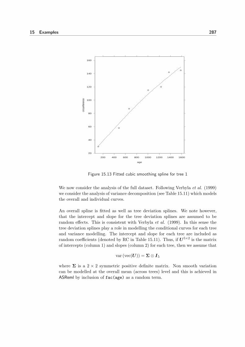
15 Examples 287

o

o

o

o

o

oo

20

40

60

80

100

120

140

160

200 400 600 800 1000 1200 1400 1600

age

circu

mfe

renc

e

Figure 15.13 Fitted cubic smoothing spline for tree 1

We now consider the analysis of the full dataset. Following Verbyla et al. (1999)we consider the analysis of variance decomposition (see Table 15.11) which modelsthe overall and individual curves.

An overall spline is fitted as well as tree deviation splines. We note however,that the intercept and slope for the tree deviation splines are assumed to berandom effects. This is consistent with Verbyla et al. (1999). In this sense thetree deviation splines play a role in modelling the conditional curves for each treeand variance modelling. The intercept and slope for each tree are included asrandom coefficients (denoted by RC in Table 15.11). Thus, if U5×2 is the matrixof intercepts (column 1) and slopes (column 2) for each tree, then we assume that

var (vec(U)) = Σ⊗ I5

where Σ is a 2 × 2 symmetric positive definite matrix. Non smooth variationcan be modelled at the overall mean (across trees) level and this is achieved inASReml by inclusion of fac(age) as a random term.

15 Examples 288

Table 15.11 Orange data: AOV decomposition

stratum decomposition type df or ne

constant 1 F 1age

age F 1spl(age,7) R 5fac(age) R 7

treetree RC 5

age.treex.tree RC 5spl(age,7).tree R 25

error R

An extract of the ASReml input file is

circ ~ mu age !r Tree 4.6 Tree.age .000094 spl(age,7) .1,

spl(age,7).Tree 2.3 fac(age) 13.9

0 0 1

Tree 2

2 0 US 4.6 .00001 .000094

5 0 0

predict age Tree !IGNORE fac(age)

We stress the importance of model building in these settings, where we generallycommence with relatively simple variance models and update to more complexvariance models if appropriate. Table 15.12 presents the sequence of fitted mod-els we have used. Note that the REML log-likelihoods for models 1 and 2 arecomparable and likewise for models 3 to 6. The REML log-likelihoods are notcomparable between these groups due to the inclusion of the fixed season termin the second set of models.

We begin by modelling the variance matrix for the intercept and slope for eachtree, Σ, as a diagonal matrix as there is no point including a covariance com-ponent between the intercept and slope if the variance component(s) for one (orboth) is zero. Model 1 also does not include a non-smooth component at theoverall level (that is, fac(age)). Abbreviated output is shown below.

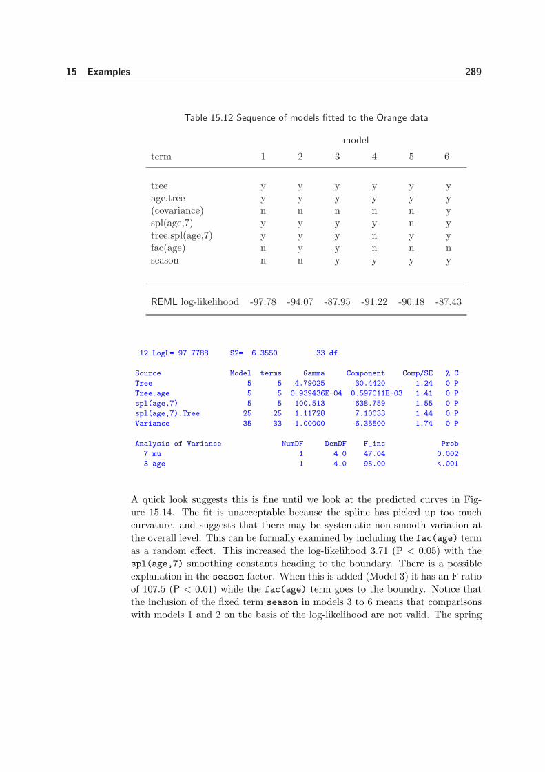
15 Examples 289

Table 15.12 Sequence of models fitted to the Orange data

model

term 1 2 3 4 5 6

tree y y y y y yage.tree y y y y y y(covariance) n n n n n yspl(age,7) y y y y n ytree.spl(age,7) y y y n y yfac(age) n y y n n nseason n n y y y y

REML log-likelihood -97.78 -94.07 -87.95 -91.22 -90.18 -87.43

12 LogL=-97.7788 S2= 6.3550 33 df

Source Model terms Gamma Component Comp/SE % C

Tree 5 5 4.79025 30.4420 1.24 0 P

Tree.age 5 5 0.939436E-04 0.597011E-03 1.41 0 P

spl(age,7) 5 5 100.513 638.759 1.55 0 P

spl(age,7).Tree 25 25 1.11728 7.10033 1.44 0 P

Variance 35 33 1.00000 6.35500 1.74 0 P

Analysis of Variance NumDF DenDF F_inc Prob

7 mu 1 4.0 47.04 0.002

3 age 1 4.0 95.00 <.001

A quick look suggests this is fine until we look at the predicted curves in Fig-ure 15.14. The fit is unacceptable because the spline has picked up too muchcurvature, and suggests that there may be systematic non-smooth variation atthe overall level. This can be formally examined by including the fac(age) termas a random effect. This increased the log-likelihood 3.71 (P < 0.05) with thespl(age,7) smoothing constants heading to the boundary. There is a possibleexplanation in the season factor. When this is added (Model 3) it has an F ratioof 107.5 (P < 0.01) while the fac(age) term goes to the boundry. Notice thatthe inclusion of the fixed term season in models 3 to 6 means that comparisonswith models 1 and 2 on the basis of the log-likelihood are not valid. The spring

15 Examples 290

Predicted values of circ

118 1582x 30

217

1 1

2 2

3 3

4 4

5 5

Figure 15.14 Plot of fitted cubic smoothing spline for model 1

measurements are lower than the autumn measurements so growth is slower inwinter. Models 4 and 5 successively examined each term, indicating that bothsmoothing constants are significant (P < 0.05). Lastly we add the covarianceparameter between the intercept and slope for each tree in model 6. This ensuresthat the covariance model will be translation invariant. A portion of the outputfile for model 6 is

8 LogL=-87.4291 S2= 5.6303 32 df

Source Model terms Gamma Component Comp/SE % C

spl(age,7) 5 5 2.17239 12.2311 1.09 0 P

spl(age,7).Tree 25 25 1.38565 7.80160 1.47 0 P

Variance 35 32 1.00000 5.63028 1.72 0 P

Tree UnStru 1 1 5.62219 31.6545 1.26 0 U

Tree UnStru 2 1 -0.124202E-01 -0.699290E-01 -0.85 0 U

Tree UnStru 2 2 0.108377E-03 0.610192E-03 1.40 0 U

Covariance/Variance/Correlation Matrix UnStructured

31.65 -0.5032

-0.6993E-01 0.6102E-03

Analysis of Variance NumDF DenDF F_inc Prob

7 mu 1 4.0 169.87 <.001

3 age 1 4.0 92.78 <.001

5 Season 1 8.9 108.60 <.001

15 Examples 291

o

oo

oo

oo

50

100

150

200

1

200 600 1000 1400

o

o

o

o

o

o o

2o

oo

oo

oo

3

o

o

o

oo

oo

50

100

150

200

4o

o

o

o

o

oo

50

100

150

200

5 Marginal

200 600 1000 1400

Time since December 31, 1968 (Days)

Tru

nk c

ircum

fere

nce

(mm

)

Figure 15.15: Trellis plot of trunk circumference for each tree at sample dates (ad-justed for season effects), with fitted profiles across time and confidence intervals

Figure 15.15 presents the predicted growth over time for individual trees and amarginal prediction for trees with approximate confidence intervals (2±× stan-dard error of prediction). Within this figure, the data is adjusted to remove theestimated seasonal effect. The conclusions from this analysis are quite differ-ent from those obtained by the nonlinear mixed effects analysis. The individualcurves for each tree are not convincingly modelled by a logistic function. Fig-ure 15.16 presents a plot of the residuals from the nonlinear model fitted on p340of Pinheiro and Bates (2000). The distinct pattern in the residuals, which is thesame for all trees is taken up in our analysis by the season term.

15 Examples 292

-10

-5

0

5

10

200 400 600 800 1000 1200 1400 1600

age

Resid

ual

Figure 15.16 Plot of the residuals from the nonlinear model of Pinheiro and Bates

15.10 Multivariate animal genetics data - Sheep

The analysis of incomplete or unbalanced multivariate data often presents com-putational difficulties. These difficulties are exacerbated by either the number ofrandom effects in the linear mixed model, the number of traits, the complexity ofthe variance models being fitted to the random effects or the size of the problem.In this section we illustrate two approaches to the analysis of a complex set ofincomplete multivariate data.

Much of the difficulty in conducting such analyses in ASReml centres on obtaininggood starting values. Derivative based algorithms such as the AI algorithm can beunreliable when fitting complex variance structures unless good starting valuesare available. Poor starting values may result in divergence of the algorithmor slow convergence. A particular problem with fitting unstructured variancemodels is keeping the estimated variance matrix positive definite. These are notsimple issues and in the following we present a pragmatic approach to them.

15 Examples 293

The data are taken from a large genetic study on Coopworth lambs. A total of 5traits, namely weaning weight (wwt), yearling weight (ywt), greasy fleece weight(gfw), fibre diameter (fdm) and ultrasound fat depth at the C site (fat) weremeasured on 7043 lambs. The lambs were the progeny of 92 sires and 3561 dams,produced from 4871 litters over 49 flock-year combinations. Not all traits weremeasured on each group. No pedigree data was available for either sires or dams.

The aim of the analysis is to estimate heritability (h2) of each trait and to estimatethe genetic correlations between the five traits. We will present two approaches,a half-sib analysis and an analysis based on the use of an animal model, whichdirectly defines the genetic covariance between the progeny and sires and dams.

The data fields included factors defining sire, dam and lamb (tag), covariates suchas age, the age of the lamb at a set time, brr the birth rearing rank (1 = bornsingle raised single, 2 = born twin raised single, 3 = born twin raised twin and 4= other), sex (M, F) and grp a factor indicating the flock-year combination.

Half-sib analysis

In the half-sib analysis we include terms for the random effects of sires, dams andlitters. In univariate analyses the variance component for sires is denoted byσ2

s = 14σ2

A where σ2A is the additive genetic variance, the variance component for

dams is denoted by σ2d = 1

4σ2A +σ2

m where σ2m is the maternal variance component

and the variance component for litters is denoted by σ2l and represents variation

attributable to the particular mating.

For a multivariate analysis these variance components for sires, dams andlitters are, in theory replaced by unstructured matrices, one for each term.Additionally we assume the residuals for each trait may be correlated. Thus forthis example we would like to fit a total of 4 unstructured variance models. Forsuch a situation, it is sensible to commence the modelling process with a series ofunivariate analyses. These give starting values for the diagonals of the variancematrices, but also indicate what variance components are estimable. The ASReml

job for the univariate analyses is

Multivariate Sire & Dam model

tag

sire 92 !I

dam 3561 !I

grp 49

sex

brr 4

litter 4871

15 Examples 294

Table 15.13: REML estimates of a subset of the variance parameters for each traitfor the genetic example, expressed as a ratio to their asymptotic s.e.

term wwt ywt gfw fdm fat

sire 3.68 3.57 3.95 1.92 1.92dam 6.25 4.93 2.78 0.37 0.05

litter 8.79 0.99 2.23 1.91 0.00age.grp 2.29 1.39 0.31 1.15 1.74sex.grp 2.90 3.43 3.70 - 1.83

Table 15.14 Wald tests of the fixed effects for each trait for the genetic example

term wwt ywt gfw fdm fat

age 331.3 67.1 52.4 2.6 7.5brr 554.6 73.4 14.9 0.3 13.9sex 196.1 123.3 0.2 2.9 0.6

age.sex 10.3 1.7 1.9 - 5.0

age wwt !M0 ywt !M0 # !M0 recodes zeros as missing values

gfw !M0 fdm !M0 fat !M0

coop.fmt

wwt ~ mu age brr sex age.sex !r sire dam lit age.grp sex.grp !f grp

Tables 15.13 and 15.14 present the summary of these analyses. Fibre diameterwas measured on only 2 female lambs and so interactions with sex were notfitted. The dam variance component was quite small for both fibre diameter andfat. The REML estimate of the variance component associated with litters waseffectively zero for fat.

Thus in the multivariate analysis we consider fitting the following models to thesire, dam and litter effects,

var (us) = Σs ⊗ I92

15 Examples 295

var (ud) = Σd ⊗ I3561

var (ul) = Σl ⊗ I4891

where Σ5×5s ,Σ3×3

d and Σ4×4l are positive definite symmetric matrices correspond-

ing to the between traits variance matrices for sires, dams and litters respectively.The variance matrix for dams does not involve fibre diameter and fat depth, whilethe variance matrix for litters does not involve fat depth. The effects in each ofthe above vectors are ordered levels within traits. Lastly we assume that theresidual variance matrix is given by

Σe ⊗ I7043

Table 15.15 presents the sequence variance models fitted to each of the fourrandom terms sire, dam, litter and error in the ASReml job

Multivariate Sire & Dam model

tag

sire 92 !I

dam 3561 !I

grp 49

sex

brr 4

litter 4871

age wwt !m0 ywt !m0 # !M0 identifies missing values

gfw !m0 fdm !m0 fat !m0

coop.fmt !DOPATH $1 !CONTINUE !MAXIT 20

!PATH 3

!EXTRA 4

!PATH

wwt ywt gfw fdm fat ~ Trait Tr.age Tr.brr Tr.sex Tr.age.sex,

!r Tr.sire,

! at(Tr,1).dam at(Tr,2).dam at(Tr,3).dam !,

! at(Tr,1).lit at(Tr,2).lit at(Tr,3).lit at(Tr,4).lit !,

at(Trait,1).age.grp .0024,

at(Trait,2).age.grp .0019,

at(Trait,4).age.grp .0020,

at(Trait,5).age.grp .00026,

at(Trait,1).sex.grp .93,

at(Trait,2).sex.grp 16.0,

at(Trait,3).sex.grp .28,

at(Trait,5).sex.grp 1.18,

!f Tr.grp

1 2 3 #1 R structure with 2 dimensions and 3 G structures

0 0 0 #Independent across animals

Tr 0 US #General structure across traits

15 Examples 296

15*0. #Asreml will estimate some starting values

Tr.sire 2 #Sire effects.

!PATH 1 #Initial analysis ignoring genetic correlations

Tr 0 DIAG #Specified diagonal variance structure

0.608 1.298 0.015 0.197 0.035 #Initial sire variances

!PATH 2 #Factor Analytic model

Tr 0 FA1 !GP

0.5 0.5 -.01 -.01 0.1 #Correlation factors

0.608 1.298 0.015 0.197 0.035 #Variances

!PATH 3 #Unstructured variance model

Tr 0 US

0.6199 #Lower triangle row-wise

0.6939 1.602

0.003219 0.007424 0.01509

-0.02532 -0.05840 -0.0002709 0.1807

0.06013 0.1387 0.0006433 -0.005061 0.03487

!PATH

sire

#Maternal structure covers the 3 model terms

# at(Tr,1).dam at(Tr,2).dam at(Tr,3).dam

at(Tr,1).dam 2 # Maternal effects.

!PATH 1

3 0 CORGH !GU # Equivalent to Unstructured

.9

.1 .1

2.2 4.14 0.018

!PATH 2

3 0 CORGH !GU

.9

.1 .1

2.2 4.14 0.018

!PATH 3

3 0 US !GU

.9

.1 .1

2.2 4.14 0.018

!PATH

dam

#Litter structure covers the 4 model terms at(Tr,1).lit at(Tr,2).lit

#at(Tr,3).lit at(Tr,4).lit

at(Tr,1).lit 2 # Litter effects.

!PATH 1

4 0 DIAG # Diagonal structure

15 Examples 297

3.74 0.97 0.019 0.941

!PATH 2

4 0 FA1 !GP # Factor Analytic 1

.5 .5 .01 .1

4.95 4.63 0.037 0.941

!PATH 3

4 0 US # Unstructured

5.073

3.545 3.914

0.1274 0.08909 0.02865

0.07277 0.05090 0.001829 1.019

!PATH

lit

Table 15.15: Variance models fitted for each part of the ASReml job in the analysisof the genetic example

term matrix !PATH 1 !PATH 2 !PATH 3

sire Σs DIAG FA1 USdam Σd CORGH CORGH US

litter Σl DIAG FA1 USerror Σe US US US

In !PATH 1, the error variance model is taken to be unstructured, but the startingvalues are set to zero. This instructs ASReml to obtain starting values from thesample covariance matrix of the data. For incomplete data the matrix so obtainedmay not, in general be positive definite. Care should be taken when using thisoption for incomplete multivariate data. The command to run !PATH 1 is

asreml -nrw64 mt 1

The Loglikelihood from this run is −20000 − 1444.93. When the job runs, themessage

Non positive definite G matrix: 0 singularities 1 negative pivots;order 3

appears to the screen. This refers to the 3× 3 dam matrix which is estimated as

15 Examples 298

Covariance/Variance/Correlation Matrix CORRelation

2.573 1.025 0.6568

3.024 3.382 0.7830

0.1526 0.2086 0.2098E-01

Note the correlation between wwt and ywt is estimated at 1.025.

The results from this analysis can be automatically used by ASReml for the nextpart, if the .rsv is copied prior to running the next part. That is, we add the!PATH 2 coding to the job, copy mt1.rsv to mt2.rsv so that when we run !PATH2 it starts from where !PATH 1 finished, and run the job using

asreml -cnrw64 mt 2

The Loglikelihood from this run is −20000− 1427.37.

Finally, we use the !PATH 3 coding to obtain the final analysis, copy mt2.rsv tomt3.rsv and run the final stage starting from the stage 2 results. Note that weare using the automatic updating associated with !CONTINUE. A portion of thefinal output file is

Notice: LogL values are reported relative to a base of -20000.00

NOTICE: 76 singularities detected in design matrix.

1 LogL=-1427.37 S2= 1.0000 35006 df : 2 components constrained

2 LogL=-1424.58 S2= 1.0000 35006 df

3 LogL=-1421.07 S2= 1.0000 35006 df : 1 components constrained

4 LogL=-1420.11 S2= 1.0000 35006 df

5 LogL=-1419.93 S2= 1.0000 35006 df

6 LogL=-1419.92 S2= 1.0000 35006 df

7 LogL=-1419.92 S2= 1.0000 35006 df

8 LogL=-1419.92 S2= 1.0000 35006 df

9 LogL=-1419.92 S2= 1.0000 35006 df

10 LogL=-1419.92 S2= 1.0000 35006 df

11 LogL=-1419.92 S2= 1.0000 35006 df

Source Model terms Gamma Component Comp/SE % C

at(Trait,1).age.grp 49 49 0.135360E-02 0.135360E-02 2.03 0 P

at(Trait,2).age.grp 49 49 0.101561E-02 0.101561E-02 1.24 0 P

at(Trait,4).age.grp 49 49 0.176505E-02 0.176505E-02 1.13 0 P

at(Trait,5).age.grp 49 49 0.209279E-03 0.209279E-03 1.68 0 P

at(Trait,1).sex.grp 49 49 0.919610 0.919610 2.89 0 P

at(Trait,2).sex.grp 49 49 15.3912 15.3912 3.50 0 P

at(Trait,3).sex.grp 49 49 0.279496 0.279496 3.71 0 P

at(Trait,5).sex.grp 49 49 1.44032 1.44032 1.80 0 P

Residual UnStru 1 1 9.46220 9.46220 33.30 0 U

: : : : :

15 Examples 299

Covariance/Variance/Correlation Matrix UnStructured Residual

9.462 0.5691 0.2356 0.1640 0.2183

7.332 17.54 0.4241 0.2494 0.4639

0.2728 0.6686 0.1417 0.3994 0.1679

0.9625 1.994 0.2870 3.642 0.4875E-01

0.8336 2.412 0.7846E-01 0.1155 1.541

Covariance/Variance/Correlation Matrix UnStructured Tr.sire

0.5941 0.7044 0.2966 0.2032 0.2703

0.6745 1.544 0.1364E-01-0.1224 0.5726

0.2800E-01 0.2076E-02 0.1500E-01 0.1121 -0.4818E-02

0.6238E-01-0.6056E-01 0.5469E-02 0.1586 -0.6331

0.3789E-01 0.1294 -0.1073E-03-0.4586E-01 0.3308E-01

Covariance/Variance/Correlation Matrix UnStructured at(Tr,1).dam

2.161 1.010 0.7663

2.196 2.186 0.8301

0.1577 0.1718 0.1959E-01

Covariance/Variance/Correlation Matrix UnStructured at(Tr,1).lit

3.547 0.5065 -0.1099 -0.4096E-01

1.555 2.657 0.1740 -0.5150

-0.2787E-01 0.3821E-01 0.1815E-01-0.3282

-0.7312E-01-0.7957 -0.4191E-01 0.8984

Analysis of Variance NumDF F_inc

15 Tr.age 5 98.95

16 Tr.brr 15 116.72

17 Tr.sex 5 59.78

19 Tr.age.sex 4 4.90

In the .res file is reported an eigen analysis of these four variance structures.

Eigen Analysis of UnStructured matrix for Residual

Eigen values 22.458 5.210 3.395 1.160 0.103

Percentage 69.474 16.118 10.502 3.588 0.318

1 0.4970 -0.8663 0.0141 0.0470 0.0027

2 0.8509 0.4765 -0.1316 -0.1746 -0.0327

3 0.0335 0.0230 0.0585 -0.0048 0.9974

4 0.1168 0.0871 0.9843 0.0769 -0.0633

5 0.1187 0.1196 -0.1010 0.9805 0.0039

Eigen Analysis of UnStructured matrix for Tr.sire

Eigen values 1.904 0.304 0.114 0.013 0.010

Percentage 81.199 12.963 4.859 0.535 0.444

1 0.4578 0.7476 0.4695 -0.1052 0.0087

2 0.8860 -0.3646 -0.2766 0.0248 -0.0700

3 0.0077 0.0798 0.0826 0.9438 -0.3098

4 -0.0163 0.5260 -0.8015 0.1116 0.2612

5 0.0710 -0.1587 0.2320 0.2918 0.9115

Eigen Analysis of UnStructured matrix for at(Tr,1).dam

15 Examples 300

Eigen values 4.382 0.010 -0.025

Percentage 100.352 0.225 -0.577

1 0.7041 -0.2321 0.6711

2 0.7081 0.1585 -0.6881

3 0.0533 0.9597 0.2760

Eigen Analysis of UnStructured matrix for at(Tr,1).lit

Eigen values 4.795 1.827 0.482 0.016

Percentage 67.345 25.664 6.769 0.221

1 0.7752 0.5928 0.2178 0.0133

2 0.6159 -0.6328 -0.4691 -0.0106

3 0.0016 -0.0340 0.0255 0.9991

4 -0.1403 0.4969 -0.8555 0.0390

The REML estimates of all the variance matrices except for the dam componentsare positive definite. Heritabilities for each trait can be calculated using the .pinfile facility of ASReml. The heritability is given by

h2 =σ2

A

σ2P

where σ2P is the phenotypic variance and is given by

σ2P = σ2

s + σ2d + σ2

l + σ2e

recalling thatσ2

s =14σ2

A

σ2d =

14σ2

A + σ2m

In the half-sib analysis we only use the estimate of additive genetic variance fromthe sire variance component. The ASReml .pin file is presented below along withthe output from the following command

asreml -p mt3

F phenWYG 9:14 + 24:29 + 39:44 + 45:50 # defines 55:60

F phenD 15:18 + 30:33 + 51:54 # defines 61:64

F phenF 19:23 + 34:38 # defines 65:69

F Direct 24:38 * 4. # defines 70:84

F Maternal 39:44 - 24:29 # defines 85:90

H WWTh2 70 55

H YWTh2 72 57

H GFWh2 75 60

H FDMh2 79 64

H FATh2 84 69

R GenCor 24:38

R MatCor 85:90

15 Examples 301

55 phenWYG 9 15.76 0.3130

56 phenWYG 10 11.76 0.3749

57 phenWYG 11 23.92 0.6313

. . . . .

70 Direct 24 2.376 0.6458

71 Direct 25 2.698 0.8487

72 Direct 26 6.174 1.585

73 Direct 27 0.1120 0.7330E-01

. . . . .

85 Maternal 39 1.567 0.3788

86 Maternal 40 1.521 0.4368

87 Maternal 41 0.6419 0.7797

. . . . .

WWTh2 = Direct 2 70/phenWYG 55= 0.1507 0.0396

YWTh2 = Direct 2 72/phenWYG 57= 0.2581 0.0624

GFWh2 = Direct 2 75/phenWYG 60= 0.3084 0.0716

FDMh2 = Direct 3 79/phenD 18 64= 0.1350 0.0717

FATh2 = Direct 3 84/phenF 23 69= 0.0841 0.0402

GenCor 2 1 = Tr.si 25/SQR[Tr.si 24*Tr.si 26]= 0.7044 0.1025

GenCor 3 1 = Tr.si 27/SQR[Tr.si 24*Tr.si 29]= 0.2966 0.1720

GenCor 3 2 = Tr.si 28/SQR[Tr.si 26*Tr.si 29]= 0.0136 0.1810

GenCor 4 1 = Tr.si 30/SQR[Tr.si 24*Tr.si 33]= 0.2028 0.3513

GenCor 4 2 = Tr.si 31/SQR[Tr.si 26*Tr.si 33]= -0.1227 0.3247

GenCor 4 3 = Tr.si 32/SQR[Tr.si 29*Tr.si 33]= 0.1115 0.3868

GenCor 5 1 = Tr.si 34/SQR[Tr.si 24*Tr.si 38]= 0.2703 0.2724

GenCor 5 2 = Tr.si 35/SQR[Tr.si 26*Tr.si 38]= 0.5726 0.2022

GenCor 5 3 = Tr.si 36/SQR[Tr.si 29*Tr.si 38]= -0.0048 0.2653

GenCor 5 4 = Tr.si 37/SQR[Tr.si 33*Tr.si 38]= -0.6333 0.3775

MatCor 2 1 = Mater 86/SQR[Mater 85*Mater 87]= 1.5168 0.7131

MatCor 3 1 = Mater 88/SQR[Mater 85*Mater 90]= 1.5285 1.1561

MatCor 3 2 = Mater 89/SQR[Mater 87*Mater 90]= 3.1251 2.7985

15 Examples 302

Animal model

In this section we will illustrate the use of .ped files to define the genetic pedigreestructure between animals. This is an alternate method of estimating additivegenetic variance for these data. The variance matrix of the animals (sires, damsand lambs) for which we only have data on lambs is given by

var (uA) = ΣA ⊗A−1

where A−1 is the inverse of the genetic relationship matrix. There are a totalof 10696 = 92 + 3561 + 7043 animals in the pedigree. The ASReml input file ispresented below. Note that this model is not equivalent to the sire/dam/littermodel with respect to the animal/litter components for gfw, fd and fat.

Multivariate Animal model

tag !P

sire

dam !P

grp 49

sex

brr 4

litter 4871

age wwt !m0 ywt !m0 # !M0 identifies missing values

gfw !m0 fdm !m0 fat !m0

coop.fmt # read pedigree from first three fields

coop.fmt !DOPATH $1 !CONTINUE !MAXIT 20 !STEP 0.01

# $1 allows selection of PATH as a command line argument

!PATH 3

!EXTRA 4 # Force 4 more iterations after convergence criterion met

!PATH

wwt ywt gfw fdm fat ~ Trait Tr.age Tr.brr Tr.sex Tr.age.sex,

!r Tr.tag ,

at(Tr,1).dam, at(Tr,2).dam, -at(Tr,3).dam .003,

at(Tr,1).lit, at(Tr,2).lit, at(Tr,3).lit, at(Tr,4).lit,

at(Trait,1).age.grp .0024,

at(Trait,2).age.grp .0019,

at(Trait,4).age.grp .0020,

at(Trait,5).age.grp .00026,

at(Trait,1).sex.grp .93,

at(Trait,2).sex.grp 16.0,

at(Trait,3).sex.grp .28,

at(Trait,5).sex.grp 1.18,

!f Tr.grp

1 2 3 # One multivariate R structure, 3 G structures

0 0 0 # No structure across lamb records

# First zero lets ASReml count te number of records

Tr 0 US #General structure across traits

7.66

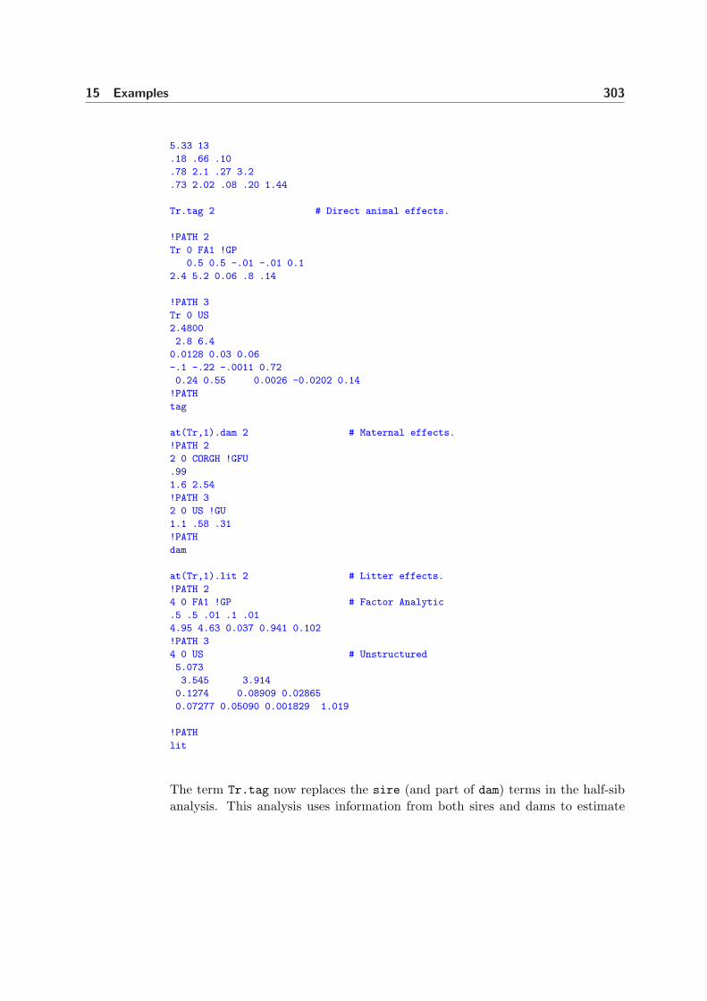
15 Examples 303

5.33 13

.18 .66 .10

.78 2.1 .27 3.2

.73 2.02 .08 .20 1.44

Tr.tag 2 # Direct animal effects.

!PATH 2

Tr 0 FA1 !GP

0.5 0.5 -.01 -.01 0.1

2.4 5.2 0.06 .8 .14

!PATH 3

Tr 0 US

2.4800

2.8 6.4

0.0128 0.03 0.06

-.1 -.22 -.0011 0.72

0.24 0.55 0.0026 -0.0202 0.14

!PATH

tag

at(Tr,1).dam 2 # Maternal effects.

!PATH 2

2 0 CORGH !GFU

.99

1.6 2.54

!PATH 3

2 0 US !GU

1.1 .58 .31

!PATH

dam

at(Tr,1).lit 2 # Litter effects.

!PATH 2

4 0 FA1 !GP # Factor Analytic

.5 .5 .01 .1 .01

4.95 4.63 0.037 0.941 0.102

!PATH 3

4 0 US # Unstructured

5.073

3.545 3.914

0.1274 0.08909 0.02865

0.07277 0.05090 0.001829 1.019

!PATH

lit

The term Tr.tag now replaces the sire (and part of dam) terms in the half-sibanalysis. This analysis uses information from both sires and dams to estimate

15 Examples 304

additive genetic variance. The dam variance component is this analysis only es-timates the maternal variance component. It is only significant for the weaningand yearling weights. The litter variation remains unchanged. The ASReml inputfile again consists of several parts, which progressively build up to fitting unstruc-tured variance models to Tr.tag, Tr.dam, Tr.litter and error. A portion of theoutput file is

tag !P

dam !P

age wwt !m0 ywt !m0

gfw !m0 fdm !m0 fat !m0

A-inverse retrieved from ainverse.bin

PEDIGREE [pcoop.fmt ] has 10696 identities, 29474 Non zero elements

QUALIFIERS: !CONTINUE !MAXIT 20 !STEP 0.01

QUALIFIERS: !EXTRA 4

QUALIFIER: !DOPATH 3 is active

Reading pcoop.fmt FREE FORMAT skipping 0 lines

Multivariate analysis of wwt ywt gfw fdm

Multivariate analysis of fat

Using 7043 records of 7043 read

Model term Size #miss #zero MinNon0 Mean MaxNon0

1 tag !P 10696 0 0 3.000 5380. 0.1070E+05

2 sire 0 0 1.000 48.06 92.00

3 dam !P 10696 0 0 1.000 5197. 0.1070E+05

:

Forming 95033 equations: 40 dense.

Initial updates will be shrunk by factor 0.010

Restarting iteration from previous solution

Notice: LogL values are reported relative to a base of -20000.00

NOTICE: 76 singularities detected in design matrix.

1 LogL=-1437.10 S2= 1.0000 35006 df : 2 components constrained

2 LogL=-1436.87 S2= 1.0000 35006 df : 3 components constrained

3 LogL=-1434.97 S2= 1.0000 35006 df : 2 components constrained

4 LogL=-1430.73 S2= 1.0000 35006 df : 2 components constrained

5 LogL=-1424.71 S2= 1.0000 35006 df : 1 components constrained

6 LogL=-1417.98 S2= 1.0000 35006 df : 1 components constrained

7 LogL=-1417.77 S2= 1.0000 35006 df : 1 components constrained

8 LogL=-1417.62 S2= 1.0000 35006 df : 1 components constrained

9 LogL=-1417.28 S2= 1.0000 35006 df

10 LogL=-1417.23 S2= 1.0000 35006 df

:

16 LogL=-1417.23 S2= 1.0000 35006 df

Source Model terms Gamma Component Comp/SE % C

at(Trait,1).age.grp 49 49 0.132682E-02 0.132682E-02 2.02 0 P

at(Trait,2).age.grp 49 49 0.908220E-03 0.908220E-03 1.15 0 P

at(Trait,4).age.grp 49 49 0.175614E-02 0.175614E-02 1.13 0 P

at(Trait,5).age.grp 49 49 0.223617E-03 0.223617E-03 1.73 0 P

15 Examples 305

at(Trait,1).sex.grp 49 49 0.902586 0.902586 2.88 0 P

at(Trait,2).sex.grp 49 49 15.3623 15.3623 3.50 0 P

at(Trait,3).sex.grp 49 49 0.280673 0.280673 3.71 0 P

at(Trait,5).sex.grp 49 49 1.42136 1.42136 1.80 0 P

Residual UnStru 1 1 7.47555 7.47555 13.86 0 U

:

Covariance/Variance/Correlation Matrix UnStructured Residual

7.476 0.4918 0.1339 0.1875 0.1333

4.768 12.57 0.4381 0.3425 0.3938

0.1189 0.5049 0.1056 0.4864 0.1298

0.9377 2.221 0.2891 3.345 0.1171

0.4208 1.612 0.4869E-01 0.2473 1.333

Covariance/Variance/Correlation Matrix UnStructured Tr.tag

3.898 0.8164 0.5763 0.3899E-01 0.6148

4.877 9.154 0.3689 -0.1849 0.7217

0.3029 0.2971 0.7085E-01-0.2415E-01 0.3041

0.6021E-01-0.4375 -0.5027E-02 0.6117 -0.4672

0.6154 1.107 0.4104E-01-0.1853 0.2570

Covariance/Variance/Correlation Matrix UnStructured at(Tr,1).dam

0.9988 0.7024

0.5881 -0.7018

Covariance/Variance/Correlation Matrix UnStructured at(Tr,1).lit

3.714 0.5511 0.1635 -0.6157E-01

2.019 3.614 0.5176 -0.4380

0.4506E-01 0.1407 0.2045E-01-0.3338

-0.1021 -0.7166 -0.4108E-01 0.7407

Analysis of Variance NumDF F_inc

15 Tr.age 5 99.16

16 Tr.brr 15 116.52

17 Tr.sex 5 59.94

19 Tr.age.sex 4 5.10

There is no guarantee that unstructured variance component matrices will bepositive definite unless !GP qualifier is set. This example highlights this issue.We used the !GU qualifier on the maternal component to obtain the matrix

[0.9988 0.58810.5881 −0.7018

].

ASReml reports the correlation as 0.7024 which it obtains by ignoring the sign in-0.7018. This is the maternal component for ywt. Since it is entirely reasonableto expect maternal influences on growth to have dissipated at 12 months of age,it would be reasonable to refit the model omitting at(Tr,2).dam and changingthe dimension of the G structure.

Bibliography

Abramowitz, M. and Stegun, I. A. (eds) (1965). Handbook of Mathematical Func-tions, Dover Publications, New York.

Breslow, N. (2003). Whither PQL?, Technical Report 192, UW BiostatisticsWorking Paper Series, University of Washington.

Breslow, N. and Lin, X. (1995). Bias correction in generalised linear mixed modelswith a single component of dispersion, Biometrika 82: 81–91.

Breslow, N. E. and Clayton, D. G. (1993). Approximate inference in generalizedlinear mixed models, Journal of the American Statistical Association 88: 9–25.

Browne, W. and Draper, D. (2004). A comparison of bayesian and likelihood-based methods for fitting multilevel models, Research Report 04-01, Not-tingham Statistics Research Report 04-01.

Butler, D. G., Cullis, B. R., Gilmour, A. R. and Gogel, B. J. (2007). Analysisof mixed models for S language environments. ASReml-R reference manual,Technical report, Queensland Department of Primary Industries.

Callens, M. and Croux, C. (2005). Performance of likelihood-based estimationmethods for multilevel binary regression models, Technical report, Dept. ofApplied Economics, Katholieke Universiteit Leuven.

Cox, D. R. and Hinkley, D. V. (1974). Theoretical Statistics, London: Chapmanand Hall.

Cox, D. R. and Snell, E. J. (1981). Applied Statistics; Principles and Examples,London: Chapman and Hall.

Cressie, N. A. C. (1991). Statistics for spatial data, New York: John Wiley andSons, Inc.

Cullis, B. R. and Gleeson, A. C. (1991). Spatial analysis of field experiments -an extension to two dimensions, Biometrics 47: 1449–1460.

306

Bibliography 307

Cullis, B. R., Gleeson, A. C., Lill, W. J., Fisher, J. A. and Read, B. J. (1989).A new procedure for the analysis of early generation variety trials, AppliedStatistics 38: 361–375.

Cullis, B. R., Gogel, B. J., Verbyla, A. P. and Thompson, R. (1998). Spatialanalysis of multi-environment early generation trials, Biometrics 54: 1–18.

Cullis, B. R., Smith, A. B. and Thompson, R. (2004). Perspectives of anova,reml and a general linear mixed model., in N. M. Adams, M. J. Crowder,D. J. Hand and D. A. Stephens (eds), Methods and Models in Statistics inhonour of Professor John Nelder FRS., pp. 53–94.

Dempster, A. P., Selwyn, M. R., Patel, C. M. and Roth, A. J. (1984). Statisti-cal and computational aspects of mixed model analysis, Applied Statistics33: 203–214.

Diggle, P. J., Ribeiro, P. J. J. and Christensen, O. F. (2003). An introduction tomodel-based geostatistics, in J. Moller (ed.), Spatial Statistics and Compu-tational Methods, Springer-Verlag, pp. 43–86.

Draper, N. R. and Smith, H. (1998). Applied Regression Analysis, John Wileyand Sons, New York, 3rd Edition.

Dutkowski, G. and Gilmour, A. R. (2001). Modification of the additive rela-tionship matrix for open pollinated trials., Developing the Eucalypt of theFuture. 10-15 September, Valdivia, Chile. p. 71.

Engel, B. (1998). A simple illustration of the failure of PQL, IRREML and APHLas approximate ml methods for mixed models for binary data, BiometricalJournal 2: 141–154.

Engel, B. and Buist, W. (1998). Bias reduction of approximate maximum like-lihood estimates for heritability in threshold models, Biometrics 54: 1155–1164.

Engel, B. and Keen, A. (1994). A simple approach for the analysis of generalizedlinear mixed models, Statistica Neerlandica 48(1): 1–22.

Fischer, T. M., Gilmour, A. R. and van der Werf, J. (2004). Computing approx-imate standard errors for genetic parameters derived from random regres-sion models fitted by average information reml, Genetics Selection Evolution36(3): 363–369.

Gilmour, A. R., Anderson, R. D. and Rae, A. L. (1985). The analysis of binomialdata by a generalised linear mixed model, Biometrika 72: 593–599.

Bibliography 308

Gilmour, A. R., Cullis, B. R. and Verbyla, A. P. (1997). Accounting for naturaland extraneous variation in the analysis of field experiments, Journal ofAgricultural, Biological and Environmental Statistics 2: 269–293.

Gilmour, A. R., Cullis, B. R., Welham, S. J., Gogel, B. J. and Thompson, R.(2004). An efficient computing strategy for prediction in mixed linear mod-els, Computational Statistics and Data Analysis 44: 571–586.

Gilmour, A. R., Thompson, R. and Cullis, B. R. (1995). AI, an efficient algorithmfor REML estimation in linear mixed models, Biometrics 51: 1440–1450.

Gleeson, A. C. and Cullis, B. R. (1987). Residual maximum likelihood (REML)estimation of a neighbour model for field experiments, Biometrics 43: 277–288.

Gogel, B. J. (1997). Spatial analysis of multi-environment variety trials, PhDthesis, Department of Statistics, University of Adelaide, South Australia.

Goldstein, H. and Rasbash, J. (1996). Improved approximations for multilevelmodels with binary response, Journal of the Royal Statistical Society A –General 159: 505–513.

Goldstein, H., Rasbash, J., Plewis, I., Draper, D., Browne, W., Yang, M., Wood-house, G. and Healy, M. (1998). A user’s guide to MLwiN, Institute ofEducation, London.

Green, P. J. and Silverman, B. W. (1994). Nonparametric regression and gener-alized linear models, London: Chapman and Hall.

Harvey, W. R. (1977). Users’ guide to LSML76, The Ohio State University,Columbus.

Harville, D. A. (1997). Matrix algebra from a statisticians perspective, Springer-Verlag, New York.

Harville, D. and Mee, R. (1984). A mixed model procedure for analysing orderedcategorical data, Biometrics 40: 393–408.

Haskard, K. A. (2006). Anisotropic Matern correlation and other issues in model-based geostatistics, PhD thesis, BiometricsSA, University of Adelaide.

Kammann, E. E. and Wand, M. P. (2003). Geoadditive models, Applied Statistics52(1): 1–18.

Bibliography 309

Keen, A. (1994). Procedure IRREML, GLW-DLO Procedure Library Manual,Agricultural Mathematics Group, Wageningen, The Netherlands, pp. Re-port LWA–94–16.

Kenward, M. G. and Roger, J. H. (1997). The precision of fixed effects estimatesfrom restricted maximum likelihood, Biometrics 53: 983–997.

Lane, P. W. and Nelder, J. A. (1982). Analysis of covariance and standardisationas instances of predicton, Biometrics 38: 613–621.

McCullagh, P. and Nelder, J. A. (1994). Generalized Linear Models, 2 edn,Chapman and Hall, London.

McCulloch, C. and Searle, S. R. (2001). Generalized, Linear, and Mixed Models,Wiley.

Millar, R. and Willis, T. (1999). Estimating the relative density of snapper in andaround a marine reserve using a log-linear mixed-effects model, Australianand New Zealand Journal of Statistics 41: 383–394.

Nelder, J. A. and Wedderburn, R. W. M. (1972). Generalised linear models,Journal of the Royal Statistical Society, Series A 135: 370–384.

Patterson, H. D. and Nabugoomu, F. (1992). REML and the analysis of seriesof crop variety trials, Proceedings from the 25th International BiometricConference, pp. 77–93.

Patterson, H. D. and Thompson, R. (1971). Recovery of interblock informationwhen block sizes are unequal, Biometrika 58: 545–54.

Piepho, H.-P., Denis, J.-B. and van Eeuwijk, F. A. (1998). Mixed biadditivemodels, Proceedings of the 28th International Biometrics Conference.

Pinheiro, J. C. and Bates, D. M. (2000). Mixed-Effects Models in S and S-PLUS,Berlin: Springer-Verlag.

R Development Core Team (2005). R: A language and environment for statisticalcomputing, R Foundation for Statistical Computing, Vienna, Austria. ISBN3-900051-07-0

Robinson, G. K. (1991). That BLUP is a good thing: The estimation of randomeffects, Statistical Science 6: 15–51.

Rodriguez, G. and Goldman, N. (2001). Improved estimation procedures formultilevel models with binary response: A case study, Journal of the RoyalStatistical Society A – General 164(2): 339–355.

Bibliography 310

Schall, R. (1991). Estimation in generalized linear models with random effects,Biometrika 78(4): 719–27.

Searle, S. R. (1971). Linear Models, New York: John Wiley and Sons, Inc.

Searle, S. R. (1982). Matrix algebra useful for statistics, New York: John Wileyand Sons, Inc.

Searle, S. R., Casella, G. and McCulloch, C. E. (1992). Variance Components,New York: John Wiley and Sons, Inc.

Self, S. C. and Liang, K. Y. (1987). Asymptotic properties of maximum likelihoodestimators and likelihood ratio tests under non-standard conditions, Journalof the American Statistical Society 82: 605–610.

Smith, A. B., Cullis, B. R., Gilmour, A. R. and Thompson, R. (1998). Multi-plicative models for interaction in spatial mixed model analyses of multi-environment trial data, Proceedings of the 28th International BiometricsConference.

Smith, A., Cullis, B. R. and Thompson, R. (2001). Analysing variety by environ-ment data using multiplicative mixed models and adjustments for spatialfield trend, Biometrics 57: 1138–1147.

Smith, A., Cullis, B. R. and Thompson, R. (2005). The analysis of crop cul-tivar breeding and evaluation trials: an overview of current mixed modelapproaches [review], Journal of Agricultural Science 143: 449–462.

Stein, M. L. (1999). Interpolation of Spatial Data: Some Theory for Kriging,Springer-Verlag, New York.

Stevens, M. M., Fox, K. M., Warren, G. N., Cullis, B. R., Coombes, N. E. andLewin, L. G. (1999). An image analysis technique for assessing resistancein rice cultivars to root-feeding chironomid midge larvae (diptera: Chirono-midae), Field Crops Research 66: 25–26.

Stroup, W. W., Baenziger, P. S. and Mulitze, D. K. (1994). Removing spatialvariation from wheat yield trials: a comparison of methods, Crop Science86: 62–66.

Thompson, R., Cullis, B. R., Smith, A. and Gilmour, A. R. (2003). A sparseimplementation of the average information algorithm for factor analyticand reduced rank variance models., Australian and New Zealand Journalof Statistics 45: 445–459.

Bibliography 311

Verbyla, A. P., Cullis, B. R., Kenward, M. G. and Welham, S. J. (1999). Theanalysis of designed experiments and longitudinal data by using smoothingsplines (with discussion), Applied Statistics 48: 269–311.

Waddington, D., Welham, S. J., Gilmour, A. R. and Thompson, R. (1994). Com-parisons of some glmm estimators for a simple binomial model., GenstatNewsletter 30: 13–24.

Webster, R. and Oliver, M. A. (2001). Geostatistics for Environmental Scientists,John Wiley and Sons, Chichester.

Welham, S. J. (1993). Genstat 5 Procedure Library manual, R. W. Payne, G.M. Arnold and G. W. Morgan, eds, release 2[3] edn, Numerical AlgorithmsGroup, Oxford.

Welham, S. J. (2005). Glmm fits a generalized linear mixed model., in R. Payneand P. Lane (eds), GenStat Reference Manual 3: Procedure Library PL17,,VSN International, Hemel Hempstead, UK, pp. 260–265.

Welham, S. J. and Thompson, R. (1997). Likelihood ratio tests for fixed modelterms using residual maximum likelihood, Journal of the Royal StatisticalSociety, Series B 59: 701–714.

Welham, S. J., Cullis, B. R., Gogel, B. J., Gilmour, A. R. and Thompson, R.(2004). Prediction in linear mixed models, Australian and New ZealandJournal of Statistics 46: 325–347.

White, I. M. S., Thompson, R. and Brotherstone, S. (1999). Genetic and environ-mental smoothing of lactation curves with cubic splines, Journal of DairyScience 82: 632–638.

Wilkinson, G. N. and Rogers, C. E. (1973). Symbolic description of factorialmodels for analysis of variance, Applied Statistics 22: 392–399.

Wolfinger, R. and O’Connell, M. (1993). Generalized linear mixed models: Apseudo-likelihood approach, Journal of Statistical Computation and Simu-lation 48: 233–243.

Wolfinger, R. D. (1996). Heterogeneous variance-covariance structures for re-peated measures, Journal of Agricultural, Biological, and EnvironmentalStatistics 1: 362–389.

Yates, F. (1935). Complex experiments, Journal of the Royal Statistical Society,Series B 2: 181–247.

Index

ABORTASR.NOW, 65

FINALASR.NOW, 65

Access, 44

accuracy - genetic BLUP, 194

advanced processing arguments, 185

AI algorithm, 13

AIC, 18

Akaike Information Criteria, 18

aliassing, 102

Analysis of Deviance, 98

animal breeding data, 2

arguments, 5

ASReml symbols

∼, 83

*, 43

., 43

#, 43

$, 43

!, 85

!, 85

*, 85

+, 85

,, 85

-, 85

/, 85

:, 85

autoregressive, 111

Average Information, 2

balanced repeated measures, 253

Bayesian Information Criteria, 18

BIC, 18

binary files, 44

Binomial divisor, 99

BLUE, 14

BLUP, 14, 15

case, 84

combining variance models, 16

command file, 30

genetic analysis, 149

multivariate, 142

Command line option

A ASK, 181

B BRIEF, 181

C CONTINUE, 183

D DEBUG, 181

F FINAL, 183

Gg graphics , 181

Hg HARDCOPY, 182

I INTERACT, 181

J JOIN, 181

N NoGraphs, 181

O ONERUN, 183

Q QUIET, 182

R RENAME, 183

S WorkSpace, 184

W WorkSpace, 184

command line options, 179

commonly used functions, 85

conditional distribution, 12

conditional factors, 90

Conditional Wald F Statistics, 20

constraining variance parameters, 137

constraints

on variance parameters, 115

contrasts, 64

Convergence criterion, 65

correlated random effects, 15

correlation, 173

between traits, 142

312

Index 313

model, 10

covariance model, 11

isotropic, 10

covariates, 42, 58, 101

cubic splines, 95

data field syntax, 48

data file, 28, 41, 42

binary format, 44

fixed format, 44

free format, 42

using Excel, 44

data file line, 32

datafile line, 59

qualifiers, 60

syntax, 59

datasets

barley.asd, 262

coop.fmt, 293

grass.asd, 253

harvey.dat, 149

nin89.asd, 28

oats.asd, 243

orange.asd, 285

rat.dat, 142

rats.asd, 247

ricem.asd, 279

voltage.asd, 250

wether.dat, 145

wheat.asd, 267

debug options, 181

Denominator Degrees of Freedom, 20

dense, 101

design factors, 101

diagnostics, 18

diallal analysis, 91

direct product, 7, 9, 106

direct sum, 9

discussion list, 4

Dispersion parameter, 98

distribution

conditional, 12

marginal, 12

Ecode, 39

Eigen analysis, 209

Eigen analysis example, 299

EM update, 134

environment variable

job control, 63

equations

mixed model, 14

error variance

heterogeneity, 9

errors, 213

Excel, 44

execution time, 209

expected information matrix, 13

F statistics, 20

Factor qualifier

DATE, 48

DMY, 49

LL Label Length, 49

MDY, 49

PRUNE, 50

SKIP fields, 50

SORT, 50

SORTALL, 50

TIME, 49

factors, 42

file

GIV, 154

pedigree, 150

Fisher-scoring algorithm, 13

fixed effects, 7

Fixed format files, 60

fixed terms, 83, 88

multivariate, 143

primary, 88

sparse, 89

Forming a job template, 34

Index 314

free format, 42

functions of variance components, 38,

170

correlation, 173

heritability, 172

linear combinations, 171

syntax, 171

G structure, 106

definition lines, 115, 120

header, 120

more than one term, 135

Gamma distribution, 98

Generalized Linear Models, 96

genetic

data, 2

groups, 152

links, 149

models, 149

qualifiers, 149

relationships, 150

GIV, 154

GLMM, 99

graphics options, 181

half-sib analysis, 293

help via email, 4

heritability, 172, 209

heterogeneity

error variance, 9

identifiable, 16

IID, 7

inbreeding coefficients, 152, 194

Incremental Wald F Statistics, 20

information matrix

expected, 13

observed, 13

initial values, 119

input file extension

.BIN, 44

.DBL, 44

.bin, 42, 44

.csv, 43

.dbl, 42, 44

.pin, 171

interactions, 90

Introduction , 19

isotropic

covariance model, 10

job control

options, 183

qualifiers, 63

key output files, 190

likelihood

log residual, 12

residual, 12

longitudinal data, 2

balanced example, 284

marginal distribution, 12

Matern variance structure, 129

measurement error, 112

MET, 9

meta analysis, 2, 9

missing values, 43, 94, 101, 195

NA, 43

in explanatory variables, 101

in response, 101

mixed

effects, 7

model, 7

mixed model, 7

equations, 14

multivariate, 143

specifying, 32

model

animal, 149, 302

correlation, 10

covariance, 11

Index 315

formulae, 83

random regression, 11

sire, 149

model building, 139

moving average, 93

multi-environment trial, 2, 9

multivariate analysis, 142, 278

example, 292

half-sib analysis, 293

Nebraska Intrastate Nursery, 27

Negative binomial distribution, 98

non singular matrices, 106

nonidentifiable, 16

objective function, 14

observed information matrix, 13

operators, 85

options

command line, 179

ordering of terms, 102

orthogonal polynomials, 94

outliers, 210

output

files, 35

multivariate analysis, 145

objects, 209

output file extension

.aov, 189, 196

.apj, 189

.asl, 189

.asp, 189

.asr, 35, 189, 190

.dbr, 189

.dpr, 189, 199

.pvc, 189

.pvs, 189, 199

.res, 189, 200

.rsv, 189, 205

.sln, 37, 189, 193

.spr, 189

.tab, 189, 207

.veo, 189

.vrb, 207

.vvp, 189, 208

.yht, 38, 189, 195

overspecified, 16

own models, 132

OWN variance structure, 131

!F2, 132

!T, 132

parameter

scale, 7

variance, 7

Path

DOPATH, 187

PATH, 187

PC environment, 177

pedigree, 149

file, 150

power, 129

Predict

!TP, 164

!TURNINGPOINTS, 164

$TP, 95

PLOT suboptions, 165

PRWTS, 167

predicted values, 38

prediction, 33, 157

qualifiers, 162

predictions

estimable, 39

prior mean, 15

product

direct, 9

qualifier

!UpArrow, 53

!<, 53

!<=, 53

!<>, 53

Index 316

!==, 53

!>, 53

!>=, 53

!*, 53

!+, 53

!-, 53

!/, 53

!=s, 133

!=, 53

!ABS, 53

!ADJUST, 73

!AILOADINGS, 79

!AISINGULARITIES, 72

!ALPHA, 152

!AOD Analysis of Deviance, 98

!ARCSIN , 53

!ARGS, 180

!ASK, 180

!ASMV, 67

!ASUV, 67

!A, 48

!BINOMIAL distribution, 98

!BLUP, 72

!BMP, 72

!BRIEF, 72, 180

!CINV, 79

!COLFAC, 67

!COMPLOGLOG , 98

!CONTINUE, 64, 139, 180

!CONTRAST, 64

!COS, 53

!CSV, 60

!CYCLE, 186

!DATAFILE, 73

!DDF, 68

!DEBUG, 180

!DEC, 164

!DENSE, 73

!DEVIANCE residuals, 99

!DF, 73

!DIAG, 152

!DISPLAY, 68

!DISP dispersion, 98

!DOM dominance, 57

!DOPART, 187

!DOPATH, 187

!D, 53

!EMFLAG , 74

!EPS, 68

!EXP, 54

!EXTRA, 75

!FACPOINTS, 80

!FCON, 65

!FILTER, 60

!FINAL, 180

!FORMAT, 60

!GAMMA distribution, 98

!GF, 133

!GIV, 152

!GKRIGE, 69

!GP, 133

!GRAPHICS, 180

!GROUPS, 153

!GU, 133

!GZ, 133

!G, 49, 66, 68

!HARDCOPY, 180

!HPGL, 69

!IDENTITY link, 98

!INBRED, 153

!INCLUDE, 63

!INTERACTIVE, 180

!I, 48

!JOIN, 66, 69, 180

!Jddm, 54

!Jmmd, 54

!Jyyd, 54

!KNOTS, 80

!LAST, 75

!LOGARITHM , 98

Index 317

!LOGFILE, 180

!LOGIT , 98

!LOGIT link, 98

!LOG link, 97

!L, 48

!MAKE, 153

!MATCH, 61

!MAXIT, 65

!MAX, 54

!MBF, 69

!MERGE, 61

!MGS, 153

!MIN, 54

!MM transformation, 54, 57

!MOD, 54

!MVREMOVE, 69

!M, 54

!NA, 54

!NEGBIN distribution, 98

!NOCHECK, 80

!NOGRAPHS, 180

!NOREORDER, 80

!NORMAL, 54

!NORMAL distribution, 97

!NOSCRATCH, 80

!OFFSET variable, 99

!ONERUN, 180

!OWN, 75

!PEARSON residuals, 99

!PLOT, 164

!POISSON distribution, 98

!POLPOINTS, 80

!PPOINTS, 80

!PRINTALL, 164

!PRINT, 76

!PROBIT , 98

!PS, 69

!PVAL, 70

!PVR GLM fitted values, 99

!PVSFORM, 76

!PVW GLM fitted values, 99

!P, 48

!QUIET, 180

!READ, 62

!RECODE, 62

!RENAME, 180

!REPEAT, 153

!REPLACE, 54

!REPORT, 80

!RESCALE, 54

!RESIDUALS, 76

!RESPONSE residuals, 99

!ROWFAC, 67, 70

!RREC, 62

!RSKIP, 62

!S2==1, 134

!S2==r, 134

!S2=, 134

!SAVE, 76

!SCALE, 81

!SCORE, 81

!SCREEN, 77

!SECTION, 70

!SED, 164

!SEED, 55

!SELECT, 60

!SELF, 153

!SEQ, 55

!SETN, 55

!SETU, 55

!SET, 55

!SIN, 53

!SKIP, 60, 153

!SLNFORM, 77

!SLOW, 81

!SMX, 77

!SORT, 153

!SPATIAL, 77

!SPLINE, 71

!SQRT link, 98

Index 318

!STEP, 71

!SUBSET, 71

!SUB, 55

!SUM, 66

!TABFORM, 77

!TOLERANCE, 81

!TOTAL, 98, 99

!TWOSTAGEWEIGHTS, 164

!TWOWAY, 78

!TXTFORM, 77

!UNIFORM, 55

!VCC, 78

!VGSECTORS, 78

!VPV, 165

!VRB, 81

!V, 56

!WMF, 78

!WORKSPACE, 180

!WORK residuals, 99

!X, 66

!YHTFORM, 78

!YSS, 73, 78

!YVAR, 180

!Y, 66

!TDIFF, 164

qualifiers

datafile line, 60

genetic, 149

job control, 63

variance model, 133

R structure, 106

definition, 118

definition lines, 115

random

effects, 7

correlated, 15

regressions

model , 11

terms

multivariate, 143

random regressions, 136

random terms, 83, 89

RCB, 31

analysis, 107

design, 28

reading the data, 31, 47

REML, i, 2, 11, 17

REMLRT, 17

repeated measures, 2, 253

reserved terms, 85

Trait, 85, 95

a(t,r), 91

and(t,r), 86, 91

at(), 92

at(f,n), 85, 92

cos(v,r), 86, 92

fac(v,y), 85, 92

fac(v), 85, 92

g(f,n), 92

giv(f,n), 86, 92

h(), 93

i(f), 93

ide(f), 86, 93

inv(v,r), 86, 93

l(f), 93

leg(v,n), 86, 93

lin(f), 85, 93

log(v,r), 86, 93

ma1(f), 86, 93

ma1, 86, 93

mu, 85, 93

mv, 85, 94

out(), 94

p(v,n), 94

pol(v,n), 87, 94

pow(x,p,o), 95

qtl(), 95

s(v [,k ]), 95

sin(v,r), 87, 95

spl(v [,k ]), 85, 95

Index 319

sqrt(v,r), 87, 95

uni(f,k), 96

uni(f,n), 87

uni(f), 87

units, 85, 95

xfa(f,k), 87, 96

reserved words

AEXP, 123

AGAU, 124

AINV, 125

ANTE[1], 124

AR2, 121

AR3, 121

ARMA, 122

AR[1], 121

CHOL[1]C, 124

CHOL[1], 124

CIR, 123

CORB, 122

CORGB, 122

CORGH, 122

CORU, 122

DIAG, 124

EXP, 122

FACV[1], 125

FA[1], 125

GAU, 123

GIV, 125

IDH, 124

ID, 121

IEUC, 123

IEXP, 123

IGAU, 123

LVR, 123

MA2, 122

MAT, 124

MA[1], 122

OWN, 124

SAR2, 121

SAR, 121

SPH, 123

US, 124

XFA[1], 125

residual

error, 7

likelihood, 12

response, 83

running the job, 33

scale parameter, 7

score, 13

Score test, 66

section, 9

separability, 10

separable, 111

singularities, 102

sparse, 101

sparse fixed, 83

spatial

analysis, 261

data, 2

model, 110

specifying the data, 47

split plot design, 242

tabulation, 32

qualifiers, 157

syntax, 157

tests of hypotheses, 19

title line, 31, 47

trait, 42, 142

transformation, 50

syntax, 52

typographic conventions, 5

unbalanced

data, 250

nested design, 246

UNIX, 177

unreplicated trial, 267

variance

Index 320

parameter, 7

variance components

functions of, 170

variance header line, 115, 117

variance model

combining, 16, 134

description, 120

forming from correlation models,

126

qualifiers, 133

specification, 106

specifying, 107

variance parameters, 11

constraining, 115, 137

between structures , 138

equality , 137

variance structures, 33, 115

multivariate, 144

Wald F tests, 20

weight, 83, 96

weights, 42

workspace options, 183